Greedy Feature Selection for Subspace Clusteringeld1/pubs/GreedyFeatureSelect.pdf · Greedy Feature Selection for Subspace Clustering a nity (LSA) (Yan and Pollefeys, 2006), spectral

Greedy Feature Selection for Subspace Clustering


Eva L. Dyer [email protected] of Electrical & Computer EngineeringRice University, Houston, TX, 77005, USA

Aswin C. Sankaranarayanan [email protected] of Electrical & Computer EngineeringCarnegie Mellon University, Pittsburgh, PA, 15213, USA

Richard G. Baraniuk [email protected]

Department of Electrical & Computer Engineering

Rice University, Houston, TX, 77005, USA

Editor:

Abstract

Unions of subspaces provide a powerful generalization of single subspace models for col-lections of high-dimensional data; however, learning multiple subspaces from data is chal-lenging due to the fact that segmentation—the identification of points that live in thesame subspace—and subspace estimation must be performed simultaneously. Recently,sparse recovery methods were shown to provide a provable and robust strategy for exactfeature selection (EFS)—recovering subsets of points from the ensemble that live in thesame subspace. In parallel with recent studies of EFS with `1-minimization, in this paper,we develop sufficient conditions for EFS with a greedy method for sparse signal recoveryknown as orthogonal matching pursuit (OMP). Following our analysis, we provide an em-pirical study of feature selection strategies for signals living on unions of subspaces andcharacterize the gap between sparse recovery methods and nearest neighbor (NN)-basedapproaches. In particular, we demonstrate that sparse recovery methods provide significantadvantages over NN methods and that the gap between the two approaches is particularlypronounced when the sampling of subspaces in the dataset is sparse. Our results suggestthat OMP may be employed to reliably recover exact feature sets in a number of regimeswhere NN approaches fail to reveal the subspace membership of points in the ensemble.

Keywords: Subspace clustering, unions of subspaces, hybrid linear models, sparse ap-proximation, structured sparsity, nearest neighbors, low-rank approximation

1. Introduction

With the emergence of novel sensing systems capable of acquiring data at scales rangingfrom the nano to the peta, modern sensor and imaging data are becoming increasingly high-dimensional and heterogeneous. To cope with this explosion of high-dimensional data, onemust exploit the fact that low-dimensional geometric structure exists amongst collectionsof data.

Linear subspace models are one of the most widely used signal models for collections ofhigh-dimensional data, with applications throughout signal processing, machine learning,and the computational sciences. This is due in part to the simplicity of linear models but

1

Dyer, Sankaranarayanan, and Baraniuk

also due to the fact that principal components analysis (PCA) provides a closed-form andcomputationally efficient solution to the problem of finding an optimal low-rank approxi-mation to a collection of data (an ensemble of signals in Rn). More formally, if we stack acollection of d vectors (points) in Rn into the columns of Y ∈ Rn×d, then PCA finds thebest rank-k estimate of Y by solving

(PCA) minX∈Rn×d

n∑i=1

d∑j=1

(Yij −Xij)2 subject to rank(X) ≤ k, (1)

where Xij is the (i, j) entry of X.

1.1 Unions of Subspaces

In many cases, a linear subspace model is sufficient to characterize the intrinsic structureof an ensemble; however, in many emerging applications, a single subspace is not enough.Instead, ensembles can be modeled as living on a union of subspaces or a union of affineplanes of mixed or equal dimension. Formally, we say that a set of d signals Y = y1, . . . , yd,each of dimension n, lives on a union of p subspaces if Y ⊂ U = ∪pi=1Si, where Si is asubspace of Rn.

Ensembles ranging from collections of images taken of objects under different illumina-tion conditions (Basri and Jacobs, 2003; Ramamoorthi, 2002), motion trajectories of point-correspondences (Kanatani, 2001), to structured sparse and block-sparse signals (Lu andDo, 2008; Blumensath and Davies, 2009; Baraniuk et al., 2010) are all well-approximated bya union of low-dimensional subspaces or a union of affine hyperplanes. Union of subspacemodels have also found utility in the classification of signals collected from complex andadaptive systems at different instances in time, e.g., electrical signals collected from thebrain’s motor cortex (Gowreesunker et al., 2011).

1.2 Exact Feature Selection

Unions of subspaces provide a natural extension to single subspace models, but providingan extension of PCA that leads to provable guarantees for learning multiple subspaces ischallenging. This is due to the fact that subspace clustering—the identification of pointsthat live in the same subspace—and subspace estimation must be performed simultaneously.However, if we can sift through the points in the ensemble and identify subsets of pointsthat lie along or near the same subspace, then a local subspace estimate1 formed from anysuch set is guaranteed to coincide with one of the true subspaces present in the ensemble(Vidal et al., 2005; Vidal, 2011). Thus, to guarantee that we obtain an accurate estimate ofthe subspaces present in a collection of data, we must select a sufficient number of subsets(feature sets) containing points that lie along the same subspace; when a feature set containspoints from the same subspace, we say that exact feature selection (EFS) occurs.

A common heuristic used for feature selection is to simply select subsets of points thatlie within an Euclidean neighborhood of one another (or a fixed number of nearest neighbors(NNs)). Methods that use sets of NNs to learn a union of subspaces include: local subspace

1. A local subspace estimate is a low-rank approximation formed from a subset of points in the ensemble,rather than from the entire collection of data.

2


affinity (LSA) (Yan and Pollefeys, 2006), spectral clustering based on locally linear approxi-mations (Arias-Castro et al., 2011), spectral curvature clustering (Chen and Lerman, 2009),and local best-fit flats (Zhang et al., 2012). When the subspaces present in the ensemble arenon-intersecting and densely sampled, NN-based approaches provide high rates of EFS andin turn, provide accurate local estimates of the subspaces present in the ensemble. However,such approaches quickly fail as the intersection between pairs of subspaces increases andas the number of points in each subspace decreases; in both of these cases, the Euclideandistance between points becomes a poor predictor of whether points belong to the samesubspace.

1.3 Endogenous Sparse Recovery

Instead of computing local subspace estimates from sets of NNs, Elhamifar and Vidal (2009)propose a novel approach for feature selection based upon forming sparse representationsof the data via `1-minimization. The main intuition underlying their approach is thatwhen a sparse representation of a point is formed with respect to the remaining pointsin the ensemble, the representation should only consist of other points that belong to thesame subspace. Under certain assumptions on both the sampling and “distance betweensubspaces”,2 this approach to feature selection leads to provable guarantees that EFS willoccur, even when the subspaces intersect (Elhamifar and Vidal, 2010; Soltanolkotabi andCandes, 2012).

We refer to this application of sparse recovery as endogenous sparse recovery due to thefact that representations are not formed from an external collection of primitives (such as abasis or dictionary) but are formed “from within” the data. Formally, for a set of d signalsY = y1, . . . , yd, each of dimension n, the sparsest representation of the ith point yi ∈ Rnis defined as

c∗i = arg minc∈Rd

‖c‖0 subject to yi =∑j 6=i

c(j)yj , (2)

where ‖c‖0 counts the number of non-zeroes in its argument and c(j) ∈ R denotes thecontribution of the jth point yj to the representation of yi. Let Λ(i) = supp(c∗i ) denote thesubset of points selected to represent the ith point and c∗i (j) denote the contribution of thejth point to the endogenous representation of yi. By penalizing representations that requirea large number of non-zero coefficients, the resulting representation will be sparse.

In general, finding the sparsest representation of a signal has combinatorial complex-ity; thus, sparse recovery methods such as basis pursuit (BP) (Chen et al., 1998) or low-complexity greedy methods (Davis et al., 1994) are employed to obtain approximate solu-tions to (2).

1.4 Contributions

In parallel with recent studies of feature selection with `1-minimization (Elhamifar andVidal, 2010; Soltanolkotabi and Candes, 2012; Elhamifar and Vidal, 2013), in this paper, westudy feature selection with a greedy method for sparse signal recovery known as orthogonal

2. The distance between a pair of subspaces is typically measured with respect to the principal anglesbetween the subspaces or other related distances on the Grassmanian manifold.

3


r(Y i)

covering radius

inra

dius

deep hole

Figure 1: Covering radius of points in a normalized subspace. The interior of the antipodalconvex hull of points in a normalized subspace—a subspace of Rn mapped to theunit `2-sphere—is shaded. The vector in the normalized subspace (unit circle)that attains the covering radius (deep hole) is marked with a star: when comparedwith the convex hull, the deep hole coincides with the maximal gap between theconvex hull and the set of all vectors that live in the normalized subspace.

matching pursuit (OMP). The main result of our analysis is a new geometric condition(Thm. 1) for EFS with OMP that highlights the tradeoff between the: mutual coherenceor similarity between points living in different subspaces and the covering radius of thepoints within the same subspace. The covering radius can be interpreted as the radiusof the largest ball that can be embedded within each subspace without touching a pointin the ensemble; the vector that lies at the center of this open ball, or the vector in thesubspace that attains the covering radius is referred to as a deep hole. Thm. 1 suggests thatsubspaces can be arbitrarily close to one another and even intersect, as long as the data isdistributed “nicely” along each subspace. By “nicely”, we mean that the points that lie oneach subspace do not cluster together, leaving large gaps in the sampling of the underlyingsubspace. In Fig. 1, we illustrate the covering radius of a set of points on the sphere (thedeep hole is denoted by a star).

After introducing a general geometric condition for EFS, we extend this analysis to thecase where the data live on what we refer to as a bounded union of subspaces (Thm. 3).In particular, we show that when the points living in a particular subspace are incoherentwith the principal vectors that support pairs of subspaces in the ensemble, EFS can beguaranteed, even when non-trivial intersections exist between subspaces in the ensemble.

4


Our condition for bounded subspaces suggests that, in addition to properties related tothe sampling of subspaces, one can characterize the separability of pairs of subspaces byexamining the correlation between the dataset and the unique set of principal vectors thatsupport pairs of subspaces in the ensemble.

In addition to providing a theoretical analysis of EFS with OMP, the other main contri-bution of this work is revealing the gap between nearest neighbor-based (NN) approachesand sparse recovery methods, i.e., OMP and BP, for feature selection. In both syntheticand real world experiments, we observe that while OMP, BP, and NN provide comparablerates of EFS when subspaces in the ensemble are non-intersecting and densely sampled,sparse recovery methods provide significantly higher rates of EFS than NN sets when: (i)the dimension of the intersection between subspaces increases and (ii) the sampling densitydecreases (fewer points per subspace). In Section 5.4, we study the performance of OMP,BP, and NN-based subspace clustering on real data, where the goal is to cluster a collectionof images into their respective illumination subspaces. We show that clustering the datawith OMP-based feature selection (see Alg. 2) provides improvements over NN and BP-based (Elhamifar and Vidal, 2010, 2013) clustering methods. In the case of very sparselysampled subspaces, where the subspace dimension equals 5 and the number of points persubspace equals 16, we obtain a 10% and 30% improvement in classification accuracy withOMP (90%), when compared with BP (80%) and NN (60%).

1.5 Paper Organization

We now provide a roadmap for the rest of the paper.

Section 2. We introduce a signal model for unions of subspaces, detail the sparse subspaceclustering (SSC) algorithm (Elhamifar and Vidal, 2010), and then go on to introduce theuse of OMP for feature selection and subspace clustering (Alg. 2); we end with a motivatingexample.

Section 3 and 4. We provide a formal definition of EFS and then develop the maintheoretical results of this paper. We introduce sufficient conditions for EFS to occur withOMP for general unions of subspaces in Thm. 1, disjoint unions in Cor. 1, and boundedunions in Thm. 3.

Section 5. We conduct a number of numerical experiments to validate our theoryand compare sparse recovery methods (OMP and BP) with NN-based feature selection.Experiments are provided for both synthetic and real data.

Section 6. We discuss the implications of our theoretical analysis and empirical results onsparse approximation, dictionary learning, and compressive sensing. We conclude with anumber of interesting open questions and future lines of research.

Section 7. We supply the proofs of the results contained in Sections 3 and 4.

5


1.6 Notation

In this paper, we will work solely in real finite-dimensional vector spaces, Rn. We writevectors x in lowercase script, matrices A in uppercase script, and scalar entries of vectorsas x(j). The standard p-norm is defined as

‖x‖p =

( n∑j=1

|x(j)|p)1/p

,

where p ≥ 1. The “`0-norm” of a vector x is defined as the number of non-zero elements inx. The support of a vector x, often written as supp(x), is the set containing the indices of itsnon-zero coefficients; hence, ‖x‖0 = |supp(x)|. We denote the Moore-Penrose pseudoinverseof a matrix A as A†. If A = UΣV T then A† = V Σ+UT , where we obtain Σ+ by taking thereciprocal of the entries in Σ, leaving the zeros in their places, and taking the transpose. Anorthonormal basis (ONB) Φ that spans the subspace S of dimension k satisfies the followingtwo properties: ΦTΦ = Ik and range(Φ) = S, where Ik is the k × k identity matrix. Let

PΛ = XΛX†Λ denote an ortho-projector onto the subspace spanned by the sub-matrix XΛ.

2. Sparse Feature Selection for Subspace Clustering

In this section, we introduce a signal model for unions of subspaces, detail the sparsesubspace clustering (SSC) method (Elhamifar and Vidal, 2009), and introduce OMP-basedsparse feature selection for subspace clustering (SSC-OMP).

2.1 Signal Model

Given a set of p subspaces of Rn, S1, . . . ,Sp, we generate a “subspace cluster” by sampling

di points from the ith subspace Si of dimension ki ≤ k. Let Yi denote the set of points inthe ith subspace cluster and let Y = ∪pi=1Yi denote the union of p subspace clusters. Each

point in Y is mapped to the unit sphere to generate a union of normalized subspace clusters.Let

Y =

y1

‖y1‖2,y2

‖y2‖2, · · · , yd

‖yd‖2

denote the resulting set of unit norm points and let Yi be the set of unit norm points thatlie in the span of subspace Si. Let Y−i = Y \ Yi denote the set of points in Y with thepoints in Yi excluded.

Let Y = [Y1 Y2 · · · Yp] denote the matrix of normalized data, where each point in Yi isstacked into the columns of Yi ∈ Rn×di . The points in Yi can be expanded in terms of anONB Φi ∈ Rn×ki that spans Si and subspace coefficients Ai = ΦT

i Yi, where Yi = ΦiAi. LetY−i denote the matrix containing the points in Y with the sub-matrix Yi excluded.

2.2 Sparse Subspace Clustering

The sparse subspace clustering (SSC) algorithm (Elhamifar and Vidal, 2009) proceeds bysolving the following basis pursuit (BP) problem for each point in Y:


‖c‖1 subject to yi =∑j 6=i

c(j)yj . (3)

6


Algorithm 1 : Orthogonal Matching Pursuit (OMP)

Input: Input signal y ∈ Rn, a matrix A ∈ Rn×d containing d signals aidi=1 in itscolumns, and a stopping criterion (either the sparsity k or the approximation error κ).Output: An index set Λ containing the indices of all atoms selected in the pursuit anda coefficient vector c containing the coefficients associated with of all atoms selected inthe pursuit.

Initialize: Set the residual to the input signal s = y.1. Select the atom that is maximally correlated with the residual and add it to Λ

Λ← Λ ∪ arg maxi|〈ai, s〉|.

2. Update the residual by projecting s into the space orthogonal to the span of AΛ

s← (I − PΛ)y.

3. Repeat steps (1)–(2) until the stopping criterion is reached, e.g., either |Λ| = kor the norm of the residual ‖s‖2 ≤ κ.

4. Return the support set Λ and coefficient vector c = A†Λy.

After solving BP for each point in the ensemble, each d-dimensional feature vector c∗i isplaced into the ith row or column of a matrix C ∈ Rd×d and spectral clustering (Shi andMalik, 2000; Ng et al., 2002) is performed on the graph Laplacian of the affinity matrixW = |C|+ |CT |.

In situations where points might not admit an exact representation with respect to otherpoints in the ensemble, an inequality constrained version of BP known as basis pursuitdenoising (BPDN) may be employed for feature selection (Elhamifar and Vidal, 2013). Inthis case, the following BPDN problem is computed for each point in Y:


‖c‖1 subject to ‖yi −∑j 6=i

c(j)yj‖2 < κ, (4)

where κ is a parameter that is selected based upon the amount of noise in the data. Re-cently, Wang and Xu (2013) provided an analysis of EFS for a unconstrained variant of theformulation in (4) for noisy unions of subspaces. Soltanolkotabi et al. (2013) proposed a ro-bust procedure for subspace clustering from noisy data that extends the BPDN frameworkstudied in (Elhamifar and Vidal, 2013; Wang and Xu, 2013).

2.3 Greedy Feature Selection

Instead of solving the sparse recovery problem in (2) via `1-minimization, we propose theuse of a low-complexity method for sparse recovery known as orthogonal matching pursuit(OMP). We detail the OMP algorithm in Alg. 1. For each point yi, we solve Alg. 1 toobtain a sparse representation of the signal with respect to the remaining points in Y . Theoutput of the OMP algorithm is a feature set, Λ(i), which indexes the columns in Y selectedto form an endogenous representation of yi.

7


Algorithm 2 : Sparse Subspace Clustering with OMP (SSC-OMP)

Input: A dataset Y ∈ Rn×d containing d points yidi=1 in its columns, a stoppingcriterion for OMP, and the number of clusters p.Output: A set of d labels L = `(1), `(2), . . . , `(d), where `(i) ∈ 1, 2, . . . , p is the labelassociated with the ith point yi.

Step 1. Compute Subspace Affinity via OMP1. Solve Alg.1 for the ith point yi to obtain a feature set Λ and coefficient vector c.2. For all j ∈ Λ(i), let Cij = c(j). Otherwise, set Cij = 0.3. Repeat steps (1)–(2) for all i = 1, . . . , d.

Step 2. Perform Spectral Clustering1. Symmetrize the subspace affinity matrix C to obtain W = |C|+ |CT |.2. Perform spectral clustering on W to obtain a set of d labels L.

After computing feature sets for each point in the dataset via OMP, either a spectralclustering method or a consensus-based method (Dyer, 2011) may then be employed tocluster the data. In Alg. 2, we outline a procedure for performing an OMP-based variantof the SSC algorithm that we will refer to as SSC-OMP.

2.4 Motivating Example: Clustering Illumination Subspaces

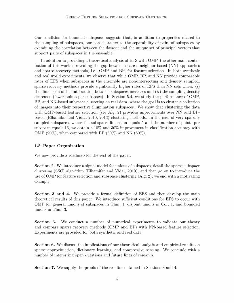
As a motivating example, we consider the problem of clustering a collection of images offaces captured under different illumination conditions: images of Lambertian objects (nospecular reflections) captured under different illumination conditions have been shown to bewell-approximated by a 5-dimensional subspace (Ramamoorthi, 2002). In Fig. 2, we showan example of the affinity matrices obtained via OMP, BP, and NN, for a collection of imagesof two faces under 64 different illumination conditions selected from the Yale B Database(Georghiades et al., 2001). In this example, each N ×N image is considered a point in RN2

and the images of a particular person’s face captured under different illumination conditionslie on a low-dimensional subspace. By varying the number of unique illumination conditionsthat we collect (number of points per subspace), we can manipulate the sampling densityof the subspaces in the ensemble. We sort the images (points) such that images of the sameface are contained in a contiguous block.

To generate the OMP affinity matrices in the right column, we use the greedy featureselection procedure outlined in Step 1 of Alg. 2, where the sparsity level k = 5. To generatethe BP affinity matrices in the middle column, we solved the BPDN problem in (4) via ahomotopy algorithm where we vary the noise parameter κ and choose the smallest value ofκ that produces up to 5 coefficients. The resulting coefficient vectors are then stacked intothe rows of a matrix C and the final subspace affinity W is computed by symmetrizing thecoefficient matrix, W = |C|+ |CT |. To generate the NN affinity matrices in the left column,we compute the absolute normalized inner products between all points in the dataset andthen threshold each row to select the k = 5 nearest neighbors to each point.

8


NN BP OMP

Figure 2: Comparison of subspace affinity matrices for illumination subspaces. In each row,we display the affinity matrices obtained for a different pair of illumination sub-spaces, for NN (left), BP (middle), and OMP (right). To the left of the affinitymatrices, we display an exemplar image from each illumination subspace.

3. Geometric Analysis of Exact Feature Selection

In this section, we provide a formal definition of EFS and develop sufficient conditions thatguarantee that EFS will occur for all of the points contained within a particular subspacecluster.

3.1 Exact Feature Selection

In order to guarantee that OMP returns a feature set (subset of points from Y) that producesan accurate local subspace estimate, we will be interested in determining when the featureset returned by Alg. 1 only contains points that belong to the same subspace cluster,i.e., exact feature selection (EFS) occurs. EFS provides a natural condition for studyingperformance of both subspace consensus and spectral clustering methods due to the factthat when EFS occurs, this results in a local subspace estimate that coincides with one ofthe true subspaces contained within the data. We now supply a formal definition of EFS.

9


Definition 1 (Exact Feature Selection) Let Yk = y : (I −Pk)y = 0, y ∈ Y index theset of points in Y that live in the span of subspace Sk, where Pk is a projector onto the spanof subspace Sk. For a point y ∈ Yk with feature set Λ, if yi ⊆ Yk, ∀i ∈ Λ, we say that Λcontains exact features.

3.2 Geometric Conditions for EFS

In this section, we develop geometric conditions that are sufficient for EFS with OMP. Beforeproceeding, however, we must introduce properties of the dataset required to develop ourmain results.

3.2.1 Preliminaries

Our main geometric result in Thm. 1 below requires measures of both the distance betweenpoints in different subspace clusters and within the same subspace cluster. A natural measureof the similarity between points living in different subspaces is the mutual coherence. Aformal definition of the mutual coherence is provided below in Def. 2.

Definition 2 (Mutual Coherence) The mutual coherence between the points in the sets(Yi,Yj) is defined as

µc(Yi,Yj) = maxu∈Yi,v∈Yj

|〈u, v〉|, where ‖u‖2 = ‖v‖2 = 1.

In words, the mutual coherence provides a point-wise measure of the normalized innerproduct (coherence) between all pairs of points that lie in two different subspace clusters.

Let µc(Yi) denote the maximum mutual coherence between the points in Yi and all othersubspace clusters in the ensemble, where

µc(Yi) = maxj 6=i

µc(Yi,Yj).

A related quantity that provides an upper bound on the mutual coherence is the cosineof the first principal angle between the subspaces. The first principal angle θ∗ij betweensubspaces Si and Sj , is the smallest angle between a pair of unit vectors (u1, v1) drawnfrom Si × Sj . Formally, the first principal angle is defined as

θ∗ij = minu∈Si, v∈Sj

arccos 〈u, v〉 subject to ‖u‖2 = 1, ‖v‖2 = 1. (5)

Whereas the mutual coherence provides a measure of the similarity between a pair ofunit norm vectors that are contained in the sets Yi and Yj , the cosine of the minimumprincipal angle provides a measure of the similarity between all pairs of unit norm vectorsthat lie in the span of Si×Sj . For this reason, the cosine of the first principal angle providesan upper bound on the mutual coherence. The following upper bound is in effect for eachpair of subspace clusters in the ensemble:

µc(Yi,Yj) ≤ cos(θ∗ij). (6)

10


To measure how well points in the same subspace cluster cover the subspace they liveon, we will study the covering radius of each normalized subspace cluster relative to theprojective distance. Formally, the covering radius of the set Yk is defined as

cover(Yk) = maxu∈Sk

miny∈Yk

dist(u, y),

where the projective distance between two vectors u and y is defined relative to the acuteangle between the vectors

dist(u, y) =

√1− |〈u, y〉|

2

‖u‖2‖y‖2.

The covering radius of the normalized subspace cluster Yi can be interpreted as the size ofthe largest open ball that can be placed in the set of all unit norm vectors that lie in thespan of Si, without touching a point in Yi.

Let (u∗i , y∗i ) denote a pair of points that attain the maximum covering diameter for Yi;

u∗i is referred to as a deep hole in Yi along Si. The covering radius can be interpreted asthe sine of the angle between the deep hole u∗i ∈ Si and its nearest neighbor y∗i ∈ Yi. Weshow the geometry underlying the covering radius in Fig. 1.

In the sequel, we will be interested in the maximum (worst-case) covering attained overall di sets formed by removing a single point from Yi. We supply a formal definition belowin Def. 3.

Definition 3 (Covering Radius) The maximum covering diameter ε of the set Yi alongthe subspace Si is defined as

ε = maxj=1,...,di

2 cover(Yi \ yj).

Hence, the covering radius equals ε/2.

A related quantity is the inradius of the set Yi, or the cosine of the angle between apoint in Yi and any point in Si that attains the covering radius. The relationship betweenthe covering diameter ε and inradius r(Yi) is given by

r(Yi) =

√1− ε2

4. (7)

A geometric interpretation of the inradius is that it measures the distance from the origin tothe maximal gap in the antipodal convex hull of the points in Yi. The geometry underlyingthe covering radius and the inradius is displayed in Fig. 1.

3.2.2 Main Result for EFS

We are now equipped to state our main result for EFS with OMP. The proof is containedin Section 7.1.

Theorem 1 Let ε denote the maximal covering diameter of the subspace cluster Yi asdefined in Def. 3. A sufficient condition for Alg. 1 to return exact feature sets for all pointsin Yi is that the mutual coherence

µc(Yi) <

√1− ε2

4− ε

4√

12maxj 6=i

cos(θ∗ij), (8)

11


where θ∗ij is the minimum principal angle defined in (5).

In words, this condition requires that the mutual coherence between points in differentsubspaces is less than the difference of two terms that both depend on the covering radiusof points along a single subspace. The first term on the RHS of (8) is equal to the inradius,as defined in (7). The second term on the RHS of (8) is the product of the cosine ofthe minimum principal angle between pairs of subspaces in the ensemble and the coveringdiameter ε of the points in Yi.

When subspaces in the ensemble intersect, i.e., cos(θ∗ij) = 1, condition (8) in Thm. 1can be simplified as

µc(Yi) <√

1− ε2

4− ε

4√

12≈√

1− ε2

4− ε

1.86.

In this case, EFS can be guaranteed for intersecting subspaces as long as the points indistinct subspace clusters are bounded away from intersections between subspaces. Whenthe covering radius shrinks to zero, Thm. 1 requires that µc < 1, or that points fromdifferent subspaces do not lie exactly in the subspace intersection, i.e., are identifiable fromone another.

3.2.3 EFS for Disjoint Subspaces

When the subspaces in the ensemble are disjoint, i.e., cos(θ∗ij) < 1, Thm. 1 can be simplifiedfurther by using the bound for the mutual coherence in (6). This simplification results inthe following corollary.

Corollary 1 Let θ∗ij denote the first principal angle between a pair of disjoint subspaces Siand Sj, and let ε denote the maximal covering diameter of the points in Yi. A sufficientcondition for Alg. 1 to return exact feature sets for all points in Yi is that

maxj 6=i

cos(θ∗ij) <

√1− ε2/4

1 + ε/ 4√

12.

3.2.4 Geometry Underlying EFS with OMP

The main idea underlying the proof of Thm. 1 is that, at each iteration of Alg. 1, we requirethat the residual used to select a point to be included in the feature set is closer to a pointin the correct subspace cluster (Yi) than a point in an incorrect subspace cluster (Y−i). Tobe precise, we require that the normalized inner product of the residual signal s and allpoints outside of the correct subspace cluster

maxy∈Y−i

|〈s, y〉|‖s‖2

< r(Yi), (9)

at each iteration of Alg. 1. To provide the result in Thm. 1, we require that (9) holds forall s ∈ Si, or all possible residual vectors.

A geometric interpretation of the EFS condition in Thm. 1 is that the orthogonal pro-jection of all points outside of a subspace must lie within the antipodal convex hull of theset of normalized points that span the subspace. To see this, consider the projection of the

12


Figure 3: Geometry underlying EFS. A union of two disjoint subspaces of different dimen-sion: the convex hull of a set of points (red circles) living on a 2D subspace isshaded (green). In (a), we show an example where EFS is guaranteed—the pro-jection of points along the 1D subspace lie inside the shaded region. In (b), weshow an example where EFS is not guaranteed—the projection of points alongthe 1D subspace lie outside the shaded region.

points in Y−i onto Si. Let z∗j denote the point on subspace Si that is closest to the signalyj ∈ Y−i,

z∗j = arg minz∈Si

‖z − yj‖2.

We can also write this projection in terms of a orthogonal projection operator Pi = ΦiΦTi ,

where Φi is an ONB that spans Si and z∗j = Piyj .

By definition, the normalized inner product of the residual with points in incorrectsubspace clusters is upper bounded as

maxyj∈Y−i

|〈s, yj〉|‖s‖2

≤ maxyj∈Y−i

|〈z∗j , yj〉|‖z∗j ‖2

= maxyj∈Y−i

cos∠z∗j , yj

Thus to guarantee EFS, we require that the cosine of the angle between all signals in Y−iand their projection onto Si is less than the inradius of Yi. Said another way, the EFScondition requires that the length of all projected points be less than the inradius of Yi.

In Fig. 3, we provide a geometric visualization of the EFS condition for a union of disjointsubspaces (union of a 1D subspace with a 2D subspace). In (a), we show an example whereEFS is guaranteed because the projection of the points outside of the 2D subspace lie wellwithin the antipodal convex hull of the points along the normalized 2D subspace (ring). In(b), we show an example where EFS is not guaranteed because the projection of the pointsoutside of the 2D subspace lie outside of the antipodal convex hull of the points along thenormalized 2D subspace (ring).

13


3.3 Connections to Previous Work

In this section, we will connect our results for OMP with previous analyses of EFS with BPfor disjoint (Elhamifar and Vidal, 2010, 2013) and intersecting (Soltanolkotabi and Candes,2012) subspaces. Following this, we will contrast the geometry underlying EFS with exactrecovery conditions used to guarantee support recovery for both OMP and BP (Tropp, 2004,2006).

3.3.1 Subspace Clustering with BP

Elhamifar and Vidal (2010) develop the following sufficient condition for EFS to occur forBP from a union of disjoint subspaces,

maxj 6=i

cos(θ∗ij) < maxYi∈Wi

σmin(Yi)√ki

, (10)

where Wi is the set of all full rank sub-matrices Yi ∈ Rn×ki of the data matrix Yi ∈ Rn×kiand σmin(Yi) is the minimum singular value of the sub-matrix Yi. Since we assume thatall of the data points have been normalized, σmin(Yi) ≤ 1; thus, the best case result thatcan be obtained is that the minimum principal angle, cos(θ∗ij) < 1/

√ki. This suggests that

the minimum principal angle of the union must go to zero, i.e., the union must consist oforthogonal subspaces, as the subspace dimension increases.

In contrast to the condition in (10), the conditions we provide in Thm. 1 and Cor. 1 donot depend on the subspace dimension. Rather, we require that there are enough points ineach subspace to achieve a sufficiently small covering; in which case, EFS can be guaranteedfor subspaces of any dimension.

Soltanolkotabi and Candes (2012) develop the following sufficient condition for EFS tooccur for BP from a union of intersecting subspaces,

µv(Yi) = maxy∈Y−i

‖V(i)T y‖∞ < r(Yi), (11)

where the matrix V(i) ∈ Rdi×n contains the dual directions (the dual vectors for each pointin Yi embedded in Rn) in its columns,3 and r(Yi) is the inradius as defined in (7). In words,(11) requires that the maximum coherence between any point in Y−i and the dual directionscontained in V(i) be less than the inradius of the points in Yi.

To link the result in (11) to our guarantee for OMP in Thm. 1, we observe that while (11)requires that µv(Yi) (coherence between a point in a subspace cluster and the dual directionsof points in a different subspace cluster) be less than the inradius, Thm. 1 requires thatthe mutual coherence µc(Yi) (coherence between two points in different subspace clusters)be less than the inradius minus an additional term that depends on the covering radius.For an arbitrary set of points that live on a union of subspaces, the precise relationshipbetween the two coherence parameters µc(Yi) and µv(Yi) is not straightforward; however,when the points in each subspace cluster are distributed uniformly and at random along

3. See Def. 2.2 for a formal definition of the dual directions and insight into the geometry underlying theirguarantees for EFS via BP Soltanolkotabi and Candes (2012).

14


each subspace, the dual directions will also be distributed uniformly along each subspace.4

In this case, µv(Yi) will be roughly equivalent to the mutual coherence µc(Yi).This simplification reveals the connection between the result in (11) for BP and the

condition in Thm. 1 for OMP. In particular, when µv(Yi) ≈ µc(Yi), our result for OMPrequires that the mutual coherence is smaller than the inradius minus an additional termthat is linear in the covering diameter ε. For this reason, our result in Thm. 1 is morerestrictive than the result provided in (11). The gap between the two bounds shrinks tozero only when the minimum principal angle θ∗ij → π/2 (orthogonal subspaces) or when thecovering diameter ε→ 0.

In our empirical studies, we find that when BPDN is tuned to an appropriate valueof the noise parameter κ, BPDN tends to produce higher rates of EFS than OMP. Thissuggests that the theoretical gap between the two approaches might not be an artifact of ourcurrent analysis; rather, there might exist an intrinsic gap between the performance of eachmethod with respect to EFS. Nonetheless, an interesting finding from our empirical studyin Section 5.4, is that despite the fact that BPDN provides better rates of EFS than OMP,OMP typically provides better clustering results than BPDN. For these reasons, we maintainthat OMP offers a powerful low-complexity alternative to `1-minimization approaches forfeature selection.

3.3.2 Exact Recovery Conditions for Sparse Recovery

To provide further intuition about EFS in endogenous sparse recovery, we will compare thegeometry underlying the EFS condition with the geometry of the exact recovery condition(ERC) for sparse signal recovery methods (Tropp, 2004, 2006).

To guarantee exact support recovery for a signal y ∈ Rn which has been synthesizedfrom a linear combination of atoms from the sub-matrix ΦΛ ∈ Rn×k, we must ensure thatour approximation of y consists solely of atoms from ΦΛ. Let ϕii/∈Λ denote the set ofatoms in Φ that are not indexed by the set Λ. The exact recovery condition (ERC) in Thm.2 is sufficient to guarantee that we obtain exact support recovery for both BP and OMP(Tropp, 2004).

Theorem 2 (Tropp, 2004) For any signal supported over the sub-dictionary ΦΛ, exactsupport recovery is guaranteed for both OMP and BP if

ERC(Λ) = maxi/∈Λ‖ΦΛ

†ϕi‖1 < 1.

A geometric interpretation of the ERC is that it provides a measure of how far a projectedatom ϕi outside of the set Λ lies from the antipodal convex hull of the atoms in Λ. Whena projected atom lies outside of the antipodal convex hull formed by the set of points inthe sub-dictionary ΦΛ, then the ERC condition is violated and support recovery is notguaranteed. For this reason, the ERC requires that the maximum coherence between theatoms in Φ is sufficiently low or that Φ is incoherent.

While the ERC condition requires a global incoherence property on all of the columns ofΦ, we can interpret EFS as requiring a local incoherence property. In particular, the EFS

4. This approximation is based upon personal correspondence with M. Soltankotabi, an author of the workin Soltanolkotabi and Candes (2012).

15


condition requires that the projection of atoms in an incorrect subspace cluster Y−i ontoSi must be incoherent with any deep holes in Yi along Si. In contrast, we require that thepoints within a subspace cluster exhibit local coherence in order to produce a small coveringradius.

4. EFS for Bounded Unions of Subspaces

In this section, we study the connection between EFS and the higher-order principal angles(beyond the minimum angle) between pairs of intersecting subspaces.

4.1 Subspace Distances

To characterize the “distance” between pairs of subspaces in the ensemble, the principalangles between subspaces will prove useful. As we saw in the previous section, the firstprincipal angle θ0 between subspaces S1 and S2 of dimension k1 and k2 is defined as thesmallest angle between a pair of unit vectors (u1, v1) drawn from S1 × S2. The vectorpair (u∗1, v

∗1) that attains this minimum is referred to as the first set of principal vectors.

The second principal angle θ1 is defined much like the first, except that the second set ofprincipal vectors that define the second principal angle are required to be orthogonal to thefirst set of principal vectors (u∗1, v

∗1). The remaining principal angles are defined recursively

in this way. The sequence of k = min(k1, k2) principal angles, θ0 ≤ θ1 ≤ · · · ≤ θk−1, isnon-decreasing and all of the principal angles lie between [0, π/2].

The definition above provides insight into what the principal angles/vectors tell us aboutthe geometry underlying a pair of subspaces; in practice, however, the principal angles arenot computed in this recursive manner. Rather, a computationally efficient way to computethe principal angles between two subspaces Si and Sj is to first compute the singular valuesof the matrix G = ΦT

i Φj , where Φi ∈ Rn×ki is an ONB that spans subspace Si. LetG = UΣV T denote the SVD of G and let σij ∈ [0, 1]k denote the singular values of G,where k = min(ki, kj) is the minimum dimension of the two subspaces. The mth smallestprincipal angle θij(m) is related to the mth largest entry of σij via the following relationship,cos(θij(m)) = σij(m). For our subsequent discussion, we will refer to the singular values ofG as the cross-spectra of the subspace pair (Si,Sj).

A pair of subspaces is said to be disjoint if the minimum principal angle is greaterthan zero. Non-disjoint or intersecting subspaces are defined as subspaces with minimumprincipal angle equal to zero. The dimension of the intersection between two subspacesis equivalent to the number of principal angles equal to zero or equivalently, the numberof entries of the cross-spectra that are equal to one. We define the overlap between twosubspaces as the rank(G) or equivalently, q = ‖σij‖0, where q ≥ dim(Si ∩ Sj).

4.2 Sufficient Conditions for EFS from Bounded Unions

The sufficient conditions for EFS in Thm. 1 and Cor. 1 reveal an interesting relationshipbetween the covering radius, mutual coherence, and the minimum principal angle betweenpairs of subspaces in the ensemble. However, we have yet to reveal any dependence betweenEFS and higher-order principal angles. To make this connection more apparent, we willmake additional assumptions about the distribution of points in the ensemble, namely

16


that the dataset produces a bounded union of subspaces relative to the principal vectorssupporting pairs of subspaces in the ensemble.

Let Y = [Yi Yj ] denote a collection of unit-norm data points, where Yi and Yj containthe points in subspaces Si and Sj , respectively. Let G = ΦT

i Φj = UΣV T denote the SVD

of G, where rank(G) = q. Let U = ΦiUq denote the set of left principal vectors of G that

are associated with the q nonzero singular values in Σ. Similarly, let V = ΦjVq denote theset of right principal vectors of G that are associated with the nonzero singular values in Σ.When the points in each subspace are incoherent with the principal vectors in the columnsof U and V , we say that the ensemble Y is an bounded union of subspaces. Formally, werequire the following incoherence property holds:(

‖Y Ti U‖∞, ‖Y T

j V ‖∞)≤ γ, (12)

where ‖ · ‖∞ is the entry-wise maximum and γ ∈ (0, 1]. This property requires that theinner products between the points in a subspace and the set of principal vectors that spannon-orthogonal directions between a pair of subspaces is bounded by a fixed constant.

When the points in each subspace are distributed such that (12) holds, we can rewritethe mutual coherence between any two points from different subspaces to reveal its depen-dence on higher-order principal angles. In particular, we show (in Section 7.2) that thecoherence between the residual s used in Alg. 1 to select the next point to be included inthe representation of a point y ∈ Yi, and a point in Yj is upper bounded by

maxy∈Yj

|〈s, y〉|‖s‖2

≤ γ‖σij‖1, (13)

where γ is the bounding constant of the data Y and ‖σij‖1 is the `1-norm of the cross-spectra or equivalently, the trace norm of G. Using the bound in (13), we arrive at thefollowing sufficient condition for EFS from bounded unions of subspaces. We provide theproof in Section 7.2.

Theorem 3 Let Y live on a bounded union of subspaces, where q = rank(G) and γ <√

1/q.Let σij denote the cross-spectra of the subspaces Si and Sj and let ε denote the coveringdiameter of Yi. A sufficient condition for Alg. 1 to return exact feature sets for all pointsin Yi is that the covering diameter

ε < minj 6=i

√1− γ2‖σij‖21.

This condition requires that both the covering diameter of each subspace and the bound-ing constant of the union be sufficiently small in order to guarantee EFS. One way to guar-antee that the ensemble has a small bounding constant is to constrain the total amountof energy that points in Yj have in the q-dimensional subspace spanned by the principal

vectors in V .Our analysis for bounded unions assumes that the nonzero entries of the cross-spectra

are equal, and thus each pair of supporting principal vectors in V are equally importantin determining whether points in Yi will admit EFS. However, this assumption is not truein general. When the union is supported by principal vectors with non-uniform principal

17


angles, our analysis suggests that a weaker form of incoherence is required. Instead ofrequiring incoherence with all principal vectors, the data must be sufficiently incoherentwith the principal vectors that correspond to small principal angles (or large values of thecross-spectra). This means that as long as points are not concentrated along the principaldirections with small principal angles (i.e., intersections), then EFS can be guaranteed,even when subspaces exhibit non-trivial intersections. To test this prediction, we will studyEFS for a bounded energy model in Section 5.2. We show that when the dataset is sparselysampled (larger covering radius), reducing the amount of energy that points contain insubspace intersections, does in fact increase the probability that points admit EFS.

Finally, our analysis of bounded unions suggests that the decay of the cross-spectra islikely to play an important role in determining whether points will admit EFS or not. Totest this hypothesis, we will study the role that the structure of the cross-spectra plays inEFS in Section 5.3.

5. Experimental Results

In our theoretical analysis of EFS in Sections 3 and 4, we revealed an intimate connec-tion between the covering radius of subspaces and the principal angles between pairs ofsubspaces in the ensemble. In this section, we will conduct an empirical study to explorethese connections further. In particular, we will study the probability of EFS as we varythe covering radius as well as the dimension of the intersection and/or overlap betweensubspaces.

5.1 Generative Model for Synthetic Data

In order to study EFS for unions of subspaces with varied cross-spectra, we will generatesynthetic data from unions of overlapping block sparse signals.

5.1.1 Constructing Sub-dictionaries

We construct a pair of sub-dictionaries as follows: Take two subsets Ω1 and Ω2 of k signals(atoms) from a dictionary D containing M atoms dmMm=1 in its columns, where dm ∈ Rnand |Ω1| = |Ω2| = k. Let Ψ ∈ Rn×k denote the subset of atoms indexed by Ω1, and letΦ ∈ Rn×k denote the subset of atoms indexed by Ω2. Our goal is to select Ψ and Φ suchthat G = ΨTΦ is diagonal, i.e., 〈ψi, φj〉 = 0, if i 6= j, where ψi is the ith element in Ψ andφj is the jth element of Φ. In this case, the cross-spectra is defined as σ = diag(G), whereσ ∈ [0, 1]k. For each union, we fix the “overlap” q or the rank of G = ΨTΦ to a constantbetween zero (orthogonal subspaces) and k (maximal overlap).

To generate a pair of k-dimensional subspaces with a q-dimensional overlap, we can pairthe elements from Ψ and Φ such that the ith entry of the cross-spectra equals

σ(i) =

|〈ψi, φi〉| if 1 ≤ i ≤ q,0 if i = q + 1 ≤ i ≤ k.

We can leverage the banded structure of shift-invariant dictionaries, e.g., dictionarymatrices with localized Toeplitz structure, to generate subspaces with structured cross-

18


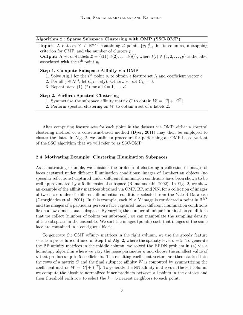
Figure 4: Generating unions of subspaces from shift-invariant dictionaries. An example ofa collection of two sub-dictionaries of five atoms, where each of the atoms havea non-zero inner product with one other atom. This choice of sub-dictionariesproduces a union of disjoint subspaces, where the overlap ratio δ = q/k = 1.

spectra as follows.5 First, we fix a set of k incoherent (orthogonal) atoms from our shift-invariant dictionary, which we place in the columns of Ψ. Now, holding Ψ fixed, we set theith atom φi of the second sub-dictionary Φ to be a shifted version of the ith atom ψi of thedictionary Ψ. To be precise, if we set ψi = dm, where dm is the mth atom in our shift-invariant dictionary, then we will set φi = dm+∆ for a particular shift ∆. By varying theshift ∆, we can control the coherence between ψi and ϕi. In Fig. 4, we show an example ofone such construction for k = q = 5. Since σ ∈ (0, 1]k, the worst-case pair of subspaces withoverlap equal to q is obtained when we pair q identical atoms with k− q orthogonal atoms.In this case, the cross-spectra attains its maximum over its entire support and equals zerootherwise. For such unions, the overlap q equals the dimension of the intersection betweenthe subspaces. We will refer to this class of block-sparse signals as orthoblock sparse signals.

5.1.2 Coefficient Synthesis

To synthesize a point that lives in the span of the sub-dictionary Ψ ∈ Rn×k, we combinethe elements ψ1, . . . , ψk and subspace coefficients α(1), . . . , α(k) linearly to form

yi =

k∑j=1

ψjα(j),

where α(j) is the subspace coefficient associated with the jth column in Ψ. Without lossof generality, we will assume that the elements in Ψ are sorted such that the values ofthe cross-spectra are monotonically decreasing. Let yci =

∑qj=1 ψjαi(j) be the “common

component” of yi that lies in the space spanned by the principal directions between the pairof subspaces that correspond to non-orthogonal principal angles between (Φ,Ψ) and letydi =

∑kj=q+1 ψjα(j) denote the “disjoint component” of yi that lies in the space orthogonal

to the space spanned by the first q principal directions.For our experiments, we consider points drawn from one of the two following coefficient

distributions, which we will refer to as (M1) and (M2) respectively.

• (M1) Uniformly Distributed on the Sphere: Generate subspace coefficients accordingto a standard normal distribution and map the point to the unit sphere

yi =

∑j ψjα(j)

‖∑j ψjα(j)‖2, where α(j) ∼ N (0, 1).

5. While shift-invariant dictionaries appear in a wide range of applications of sparse recovery (Mailhe et al.,2008; Dyer et al., 2010), we introduce the idea of using shift-invariant dictionaries to create structuredunions of subspaces for the first time here.

19


k =50

0.1 0.3 0.5 0.7 0.9

−2.5

−2

−1.5

−1

−0.5

0

0

0.2

0.4

0.6

0.8

1

−2.5

−2

−1.5

−1

−0.5

0

0.1 0.3 0.5 0.7 0.9

0.2

0.4

0.6

0.8

0.1 0.3 0.5 0.7 0.9

k = 50, m= 1000

0.2

0.4

0.6

0.8

0.1 0.3 0.5 0.7 0.9

k = 20 k = 50

Figure 5: Probability of EFS for different coefficient distributions. The probability of EFSfor a union of two subspaces of dimension k = 20 (left column) and k = 50 (rightcolumn). The probability of EFS is displayed as a function of the overlap ratioδ ∈ [0, 1) and the logarithm of the oversampling ratio log(ρ) (top row) and themutual energy τ = ‖yc‖2 (bottom row) .

• (M2) Bounded Energy Model: Generate subspace coefficients according to (M1) andrescale each coefficient in order to bound the energy in the common component

yi =τ yci‖yci ‖2

+(1− τ)ydi‖ydi ‖2

.

By simply restricting the total energy that each point has in its common component, thebounded energy model (M2) can be used to produce ensembles with small bounding constantto test the predictions in Thm. 3.

5.2 Phase Transitions for OMP

The goal of our first experiment is to study the probability of EFS—the probability that apoint in the ensemble admits exact features—as we vary both the number and distributionof points in each subspace as well as the dimension of the intersection between subspaces.For this set of experiments, we generate a union of orthoblock sparse signals, where theoverlap equals the dimension of the intersection.

Along the top row of Fig. 5, we display the probability of EFS for orthoblock sparse sig-nals generated according to the coefficient model (M1): the probability of EFS is computedas we vary the overlap ratio δ = q/k ∈ [0, 1] in conjunction with the oversampling ratioρ = k/d ∈ [0, 1], where q = rank(ΦT

1 Φ2) equals the dimension of the intersection betweenthe subspaces, and d is the number of points per subspace. Along the bottom row of Fig. 5,we display the probability of EFS for orthoblock sparse signals generated according to the

20


coefficient model (M2): the probability of EFS is computed as we vary the overlap ratioδ and the amount of energy τ ∈ [0, 1) each point has within its common component. Forthese experiments, the subspace dimension is set to k = 20 (left) and k = 50 (right). To seethe phase boundary that arises when we approach critical sampling (i.e., ρ ≈ 1), we displayour results in terms of the logarithm of the oversampling ratio. For these experiments, theresults are averaged over 500 trials.

As our theory predicts, the oversampling ratio has a strong impact on the degree of over-lap between subspaces that can be tolerated before EFS no longer occurs. In particular, asthe number of points in each subspace increases (covering radius decreases), the probabilityof EFS obeys a second-order phase transition, i.e., there is a graceful degradation in theprobability of EFS as the dimension of the intersection increases. When the pair of sub-spaces are densely sampled, the phase boundary is shifted all the way to δ = 0.7, where70%of the dimensions of each subspace intersect. This is due to the fact that as each subspaceis sampled more densely, the covering radius becomes sufficiently small to ensure that evenwhen the overlap between planes is high, EFS still occurs with high probability. In contrast,when the subspaces are critically sampled, i.e., the number of points per subspace d ≈ k,only a small amount of overlap can be tolerated, where δ < 0.1. In addition to shiftingthe phase boundary, as the oversampling ratio increases, the width of the transition region(where the probability of EFS goes from zero to one) also increases.

Along the bottom row of Fig. 5, we study the impact of the bounding constant on EFS,as discussed in Section 4.2. In this experiment, we fix the oversampling ratio to ρ = 0.1and vary the common energy τ in conjunction with the overlap ratio δ. By reducing thebounding constant of the union, the phase boundary for the uniformly distributed datafrom model (M1) is shifted from δ = 0.45 to δ = 0.7 for both k = 20 and k = 50. Thisresult confirms our predictions in the discussion of Thm. 3 that by reducing the amount ofenergy that points have in their subspace intersections EFS will occur for higher degrees ofoverlap. Another interesting finding of this experiment is that, once τ reaches a threshold,the phase boundary remains constant and further reducing the bounding constant has noimpact on the phase transitions for EFS.

5.3 Comparison of OMP and NN

In this section, we compare the probability of EFS for feature selection with OMP and near-est neighbors (NN). First, we compare the performance of both feature selection methodsfor unions with different cross-spectra. Second, we compare the phase transitions for unionsof orthoblock sparse signals as we vary the overlap and oversampling ratio.

For our experiments, we generate pairs of subspaces with structured cross-spectra asdescribed in Section 5.1.1. The cross-spectra arising from three different unions of block-sparse signals are displayed along the top row of Fig. 6. On the left, we show the cross-spectra for a union of orthoblock sparse signals with overlap ratio δ = 0.75, where q = 15and k = 20. The cross-spectra obtained by pairing shifted Lorentzian and exponential atomsare displayed in the middle and right columns, respectively. Along the bottom row of Fig.6, we show the probability of EFS for OMP and NN for each of these three subspace unionsas we vary the overlap q. To do this, we generate subspaces by setting their cross-spectraequal to the first q entries equal to the cross-spectra in Fig. 6 and setting the remaining k−q

21


Overlap Ratio ( )Overlap Ratio ( )

.9

.95

1

0.25 0.5 0.75 1

Probability of EFS

0.25 0.5 0.75 1

.2

.6

1

Probability of EFS

0.25 0.5 0.75 1

0

0.5

1

Probability of EFS

Overlap Ratio ( )

0 5 10 15 200

0.5

1

( = 0.75)

Singular value index

5 10 15 200

0.5

1

( = 1)


0 5 10 15 20

0.5

1

( = 1)


Figure 6: Probability of EFS for unions with structured cross-spectra. Along the top row,we show the cross-spectra for different unions of block-sparse signals. Along thebottom row, we show the probability of EFS as we vary the overlap ratio δ ∈ [0, 1]for OMP (solid) and NN (dash).

entries of the cross-spectra equal to zero. Each subspace cluster is generated by samplingd = 100 points from each subspace according to the coefficient model (M1).

This study provides a number of interesting insights into the role that higher-orderprincipal angles between subspaces play in feature selection for both sparse recovery methodsand NN. First, we observe that the gap between the probability of EFS for OMP and NN ismarkedly different for each of the three unions. In the first union of orthoblock sparse signals,the probability of EFS for OMP lies strictly above that obtained for the NN method, butthe gap between the performance of both methods is relatively small. In the second union,both methods maintain a high probability of EFS, with OMP admitting nearly perfectfeature sets even when the overlap ratio is maximal. In the third union, we observe thatthe gap between EFS for OMP and NN is most pronounced. In this case, the probability ofEFS for NN sets decreases to 0.1, while OMP admits a very high probability of EFS, evenwhen the overlap ratio is maximal. in summary, we observe that when data is distributeduniformly with respect to all of the principal directions between a pair of subspaces andthe cross-spectra is sub-linear, then EFS may be guaranteed with high probability for allpoints in the set provided the sampling density is sufficiently high. This is in agreementwith the discussion of EFS bounded unions in Section 4.2. Moreover, these results furthersupport our claims that in order to truly understand and predict the behavior of endogenoussparse recovery from unions of subspaces, we require a description that relies on the entirecross-spectra.

In Fig. 7, we display the probability of EFS for OMP (left) and sets of NN (right) aswe vary the overlap and the oversampling ratio. For this experiment, we consider unions oforthoblock sparse signals living on subspaces of dimension k = 50 and vary ρ ∈ [0.2, 0.96]

22


0.2

0.3

0.4

0.5

0.6

0.7

0.8

0.9

0.2 0.4 0.6 0.8 10

0.2

0.4

0.6

0.8

10.2

0.3

0.4

0.5

0.6

0.7

0.8

0.9

0.2 0.4 0.6 0.8 1

(a) (b)

Figure 7: Phase transitions for OMP and NN. The probability of EFS for orthoblock sparsesignals for OMP (a) and NN (b) feature sets as a function of the oversamplingratio ρ = k/d and the overlap ratio δ = q/k, where k = 20.

Table 1: Classification and EFS rates for illumination subspaces. Shown are the aggregateresults obtained over

(382

)pairs of subspaces.

and δ ∈ [1/k, 1]. An interesting result of this study is that there are regimes where theprobability of EFS equals zero for NN but occurs for OMP with a non-trivial probability. Inparticular, we observe that when the sampling of each subspace is sparse (the oversamplingratio is low), the gap between OMP and NN increases and OMP significantly outperformsNN in terms of their probability of EFS. Our study of EFS for structured cross-spectrasuggests that the gap between NN and OMP should be even more pronounced for cross-spectra with superlinear decay.

5.4 Clustering Illumination Subspaces

In this section, we compare the performance of sparse recovery methods, i.e., BP and OMP,with NN for clustering unions of illumination subspaces arising from a collection of imagesof faces under different lighting conditions. By fixing the camera center and position of thepersons face and capturing multiple images under different lighting conditions, the resultingimages can be well-approximated by a 5-dimensional subspace (Ramamoorthi, 2002).

In Fig. 2, we show three examples of the subspace affinity matrices obtained with NN,BP, and OMP for two different faces under 64 different illumination conditions from theYale Database B (Georghiades et al., 2001), where each image has been subsampled to48 × 42 pixels, with n = 2016. In all of the examples, the data is sorted such that theimages for each face are placed in a contiguous block.

23


To generate the NN affinity matrices in the left column of Fig. 2, we compute the absolutenormalized inner products between all points in the dataset and then threshold each row toselect the k = 5 nearest neighbors to each point. To generate the OMP affinity matrices inthe right column, we employ Step 1 of Alg. 2 with the maximum sparsity set to k = 5. Togenerate the BP affinity matrices in the middle column, we solved the BP denoising (BPDN)problem in (4) via a homotopy algorithm where we vary the noise parameter κ and choosethe smallest value of κ that produces k ≤ 5 coefficients.6 The resulting coefficient vectorsare then stacked into the rows of a matrix C and the final subspace affinity W is computedby symmetrizing the coefficient matrix, W = |C|+ |CT |.

After computing the subspace affinity matrix for each of these three feature selectionmethods, we employ a spectral clustering approach which partitions the data based uponthe eigenvector corresponding to the smallest nonzero eigenvalue of the graph Laplacian ofthe affinity matrix (Shi and Malik, 2000; Ng et al., 2002). For all three feature selectionmethods, we obtain the best clustering performance when we cluster the data based uponthe graph Laplacian instead of the normalized graph Laplacian (Shi and Malik, 2000). InTable 1, we display the percentage of points that resulted in EFS and the classificationerror for all pairs of

(382

)subspaces in the Yale B database. Along the top row, we display

the mean and median percentage of points that resulted in EFS for the full dataset (all 64illumination conditions), half of the dataset (32 illumination conditions selected at randomin each trial), and a quarter of the dataset (16 illumination conditions selected at random ineach trial). Along the bottom row, we display the clustering error (percentage of points thatwere incorrectly classified) for SSC-OMP, SSC, and NN-based clustering (spectral clusteringof the NN affinity matrix).

While both sparse recovery methods (BPDN and OMP) admit EFS rates that are com-parable to NN on the full dataset, we find that sparse recovery methods provide higher ratesof EFS than NN when the sampling of each subspace is sparse, i.e., the half and quarterdatasets. These results are also in agreement with our experiments on synthetic data. Asurprising result is that SSC-OMP provides better clustering performance than SSC on thisparticular dataset, even though BP provides higher rates of EFS.

6. Discussion

In this section, we provide insight into the implications of our results for different applica-tions of sparse recovery and compressive sensing. Following this, we end with some openquestions and directions for future research.

6.1 “Data Driven” Sparse Approximation

The standard paradigm in signal processing and approximation theory is to compute arepresentation of a signal in a fixed and pre-specified basis or overcomplete dictionary. Inmost cases, the dictionaries used to form these representations are designed according tosome mathematical desiderata. A more recent approach has been to learn a dictionary from

6. We also studied another variant of BPDN where we solve OMP for k = 5, compute the error of theresulting approximation, and then use this error as the noise parameter κ. However, this variant providedworse results than those reported in Table 1.

24


a collection of data, such that the data admit a sparse representation with respect to thelearned dictionary (Olshausen and Field, 1997; Aharon et al., 2006).

The applicability and utility of endogenous sparse recovery in subspace learning drawsinto question whether we can use endogenous sparse recovery for other tasks, includingapproximation and compression. The question that naturally arises is, “do we design a dic-tionary, learn a dictionary, or use the data as a dictionary?” Understanding the advantagesand tradeoffs between each of these approaches is an interesting and open question.

6.2 Learning Block-Sparse Signal Models

Block-sparse signals and other structured sparse signals have received a great deal of atten-tion over the past few years, especially in the context of compressive sensing from structuredunions of subspaces (Lu and Do, 2008; Blumensath and Davies, 2009) and in model-basedcompressive sensing (Baraniuk et al., 2010). In all of these settings, the fact that a classor collection of signals admit structured support patterns is leveraged in order to obtainimproved recovery of sparse signals in noise and in the presence of undersampling.

To exploit such structure in sparse signals—especially in situations where the structureof signals or blocks of active atoms may be changing across different instances in time, space,etc.—the underlying subspaces that the signals occupy must be learned directly from thedata. The methods that we have described for learning union of subspaces from ensembles ofdata can be utilized in the context of learning block sparse and other structured sparse signalmodels. The application of subspace clustering methods for this purpose is an interestingdirection for future research.

6.3 Beyond Coherence

While the maximum and cumulative coherence provide measures of the uniqueness of sub-dictionaries that are necessary to guarantee exact signal recovery for sparse recovery meth-ods (Tropp, 2004) , our current study suggests that examining the principal angles formedfrom pairs of sub-dictionaries could provide an even richer description of the geometricproperties of a dictionary. Thus, a study of the principal angles formed by different sub-sets of atoms from a dictionary might provide new insights into the performance of sparserecovery methods with coherent dictionaries and for compressive sensing from structuredmatrices. In addition, our empirical results in Section 5.3 suggest that there might existan intrinsic difference between sparse recovery from dictionaries that exhibit sublinear ver-sus superlinear decay in their principal angles or cross-spectra. It would be interesting toexplore whether these two “classes” of dictionaries exhibit different phase transitions forsparse recovery.

6.4 Discriminative Dictionary Learning

While dictionary learning was originally proposed for learning dictionaries that admit sparserepresentations of a collection of signals (Olshausen and Field, 1997; Aharon et al., 2006),dictionary learning has recently been employed for classification. To use learned dictionariesfor classification, a dictionary is learned for each class of training signals and then a sparserepresentation of a test signal is formed with respect to each of the learned dictionaries.

25


The idea is that the test signal will admit a more compact representation with respect tothe dictionary that was learned from the class of signals that the test signal belongs to.

Instead of learning these dictionaries independently of one another, discriminative dic-tionary learning (Mairal et al., 2008; Ramirez et al., 2010), aims to learn a collection ofdictionaries Φ1,Φ2, . . . ,Φp that are incoherent from one another. This is accomplishedby minimizing either the spectral (Mairal et al., 2008) or Frobenius norm (Ramirez et al.,2010) of the matrix product ΦT

i Φj between pairs of dictionaries. This same approach mayalso be utilized to learn sensing matrices for CS that are incoherent with a learned dictionary(Mailhe et al., 2012).

There are a number of interesting connections between discriminative dictionary learn-ing and our current study of EFS from collections of unions of subspaces. In particular, ourstudy provides new insights into the role that the principal angles between two dictionariestell us about our ability to separate classes of data based upon their sparse representations.Our study of EFS from unions with structured cross-spectra suggests that the decay ofthe cross-spectra between different data classes provides a powerful predictor of the perfor-mance of sparse recovery methods from data living on a union of low-dimensional subspaces.This suggests that in the context of discriminative dictionary learning, it might be moreadvantageous to reduce the `1-norm of the cross-spectra rather than simply minimizing themaximum coherence and/or Frobenius norm between points in different subspaces. To dothis, each class of data must first be embedded within a subspace, a ONB is formed for eachsubspace, and then the `1- norm of the cross-spectra must be minimized. An interestingquestion is how one might impose such a constraint in discriminative dictionary learningmethods.

6.5 Open Questions and Future Work

While EFS provides a natural measure of how well a feature selection algorithm will per-form for the task of subspace clustering, our empirical results suggest that EFS does notnecessarily predict the performance of spectral clustering methods when applied to the re-sulting subspace affinity matrices. In particular, we find that while OMP obtains lowerrates of EFS than BPDN on real-world data, OMP yields better clustering results on thesame dataset. Understanding where this difference in performance might arise from is aninteresting direction for future research.

Another interesting finding of our empirical study is that the gap between the rates ofEFS for sparse recovery methods and NN depends on the sampling density of each subspace.In particular, we found that for dense samplings of each subspace, the performance of NNis comparable to sparse recovery methods; however, when each subspace is more sparselysampled, sparse recovery methods provide significant gains over NN methods. This resultsuggests that endogenous sparse recovery provides a powerful strategy for clustering whenthe sampling of subspace clusters is sparse. Analyzing the gap between sparse recoverymethods and NN methods for feature selection is an interesting direction for future research.

7. Proofs

In this section, we provide proofs for main theorems in the paper.

26


7.1 Proof of Theorem 1

Our goal is to prove that, if (8) holds, then it is sufficient to guarantee that EFS occurs forevery point in Yk when OMP is used for feature selection. We will prove this by induction.

Consider the greedy selection step in OMP (see Alg. 1) for a point yi which belongs tothe subspace cluster Yk. Recall that at the mth step of OMP, the point that is maximallycorrelated with the signal residual will be selected to be included in the feature set Λ. Thenormalized residual at the mth step is computed as

sm =(I − PΛ)yi‖(I − PΛ)yi‖2

,

where PΛ = YΛY†

Λ ∈ Rn×n is a projector onto the subspace spanned by the points in thecurrent feature set Λ, where |Λ| = m− 1.

To guarantee that we select a point from Sk, we require that the following greedyselection criterion holds:

maxv∈Yk

|〈sm, v〉| > maxv/∈Yk

|〈sm, v〉|.

We will prove that this selection criterion holds at each step of OMP by developing anupper bound on the RHS (the maximum inner product between the residual and a pointoutside of Yk) and a lower bound on the LHS (the minimum inner product between theresidual and a point in Yk).

First, we will develop the upper bound on the RHS. In the first iteration, the residualis set to the signal of interest (yi). In this case, we can bound the RHS by the mutualcoherence µc = maxi 6=j µc(Yi,Yj) across all other sets

maxyj /∈Yk

|〈yi, yj〉| ≤ µc.

Now assume that at the mth iteration we have selected points from the correct subspacecluster. This implies that our signal residual still lies within the span of Yk, and thus wecan write the residual sm = z + e, where z is the closest point to sm in Yk and e is theremaining portion of the residual which also lies in Sk. Thus, we can bound the RHS asfollows

maxyj /∈Yk

|〈sm, yj〉| = maxyj /∈Yk

|〈z + e, yj〉|

≤ maxyj /∈Yk

|〈z, yj〉|+ |〈e, yj〉|

≤ µc + maxyj /∈Yk

|〈e, yj〉|

≤ µc + cos(θ0)‖e‖2‖yi‖2,

where θ0 is the minimum principal angle between Sk and all other subspaces in the ensemble.

27


Using the fact that cover(Yk) = ε/2, we can bound the `2-norm of the vector e as

‖e‖2 = ‖s− z‖2=√‖s‖22 + ‖z‖22 − 2|〈s, z〉|

≤√

2− 2√

1− (ε/2)2

=

√2−

√4− ε2.

Plugging this quantity into our expression for the RHS, we arrive at the following upperbound

maxyj /∈Yk

|〈sm, yj〉| ≤ µc + cos(θ0)

√2−

√4− ε2 < µc + cos(θ0)

ε4√

12,

where the final simplification comes from invoking the following Lemma.

Lemma 1 For 0 ≤ x ≤ 1, √2−

√4− x2 ≤ x

4√

12.

Proof of Lemma 1: We wish to develop an upper bound on the function

f(x) = 2−√

4− x2, for 0 ≤ x ≤ 1.

Thus our goal is to identify a function g(x), where f ′(x) ≤ g′(x) for 0 ≤ x ≤ 1, andg(0) = f(0). The derivative of f(x) can be upper bounded easily as follows

f ′(x) =x√

4− x2≤ x√

3, for 0 ≤ x ≤ 1.

Thus, g′(x) = x/√

3, and g(x) = x2/√

12; this ensures that f ′(x) ≤ g′(x) for 0 ≤ x ≤ 1,and g(0) = f(0). By the Fundamental Theorem of Integral Calculus, g(x) provides anupper bound for f(x) over the domain of interest where, 0 ≤ x ≤ 1. To obtain the final

result, take the square root of both sides,√

2−√

4− x2 ≤√x2/√

12 = x/ 4√

12.

Second, we will develop the lower bound on the LHS of the greedy selection criterion.To ensure that we select a point from Yk at the first iteration, we require that yi’s nearestneighbor belongs to the same subspace cluster. Let yinn denote the nearest neighbor to yi

yinn = arg maxj 6=i|〈yi, yj〉|.

If yinn and yi both lie in Yk, then the first point selected via OMP will result in EFS.Let us assume that the points in Yk admit an ε-covering of the subspace cluster Sk, or

that cover(Yk) = ε/2. In this case, we have the following bound in effect

maxyj∈Yk

|〈sm, yj〉| ≥√

1− ε2

4.

28


Putting our upper and lower bound together and rearranging terms, we arrive at ourfinal condition on the mutual coherence

µc <

√1− ε2

4− cos(θ0)

ε4√

12.

Since we have shown that this condition is sufficient to guarantee EFS at each step of Alg.1 provided the residual stays in the correct subspace, Thm. 1 follows by induction.

7.2 Proof of Theorem 3

To prove Thm. 3, we will assume that the union of subspaces is bounded in accordance with(12). This assumption enables us to develop a tighter upper bound on the mutual coherencebetween any residual signal s ∈ Si and the points in Yj . Since s ∈ Si, the residual can beexpressed as s = Φiα, where Φi ∈ Rn×ki is an ONB that spans Si and α = ΦT

i s. Similarly,we can write each point in Yj as y = Φjβ, where Φj ∈ Rn×kj is an ONB that spans Sj ,β = ΦT

j y. Let Bj = ΦTj yi

dji=1 denote the set of all subspace coefficients for all yi ∈ Yj .

The coherence between the residual and a point in a different subspace can be expandedas follows:

maxy∈Yj

|〈s, y〉|‖s‖2

= maxβ∈Bj

|〈Φiα,Φjβ〉|‖α‖2

= maxβ∈Bj

|〈α,ΦTi Φjβ〉|‖α‖2

= maxβ∈Bj

|〈α,UΣV Tβ〉|‖α‖2

= maxβ∈Bj

|〈UTα,ΣV Tβ〉|‖α‖2

≤ maxβ∈Bj

‖UTα‖∞‖α‖2

‖ΣV Tβ‖1, (14)

where the last step comes from an application of Holder’s inequality, i.e., |〈w, z〉| <‖w‖∞‖z‖1.

Now, we tackle the final term in (14), which we can write as

maxβ∈Bj

‖ΣV Tβ‖1 = maxy∈Yj‖ΣV TΦT

j y‖1 = maxy∈Yj‖Σ(ΦjV )T y‖1,

where the matrix ΦjV contains the principal vectors in subspace Sj . Thus, this term issimply a sum of weighted inner products between the principal vectors ΦjV and all of thepoints in Sj , where Σ contains the cross-spectra in its diagonal entries.

Since we have assumed that the union is bounded, this implies that the inner productbetween the first q principal vectors and the points in Yj are bounded by γ, where q =‖σij‖0 = rank(G). Let ΦjVq ∈ Rn×q be the first q singular vectors of G correspondingto the nonzero singular values in Σ and let Σq ∈ Rq×q be a diagonal matrix with thefirst q nonzero singular values of G along its diagonal. It follows that ‖Σ(ΦjV )T y‖∞ =

29


‖Σq(ΦjVq)T y‖∞ ≤ γ. Now, suppose that the bounding constant γ <

√1/q. In this case,

maxy∈Yj‖Σ(ΦjV )T y‖1 ≤ γ‖σij‖1.

Note that for bounded unions of subspaces, the term on the right can be made small byrequiring that the bounding constant γ 1. Plugging this bound into (14), we obtain thefollowing expression

maxy∈Yj

|〈s, y〉|‖r‖2

≤ γ‖σij‖1‖UTα‖∞‖α‖2

= γ‖σij‖1‖U‖2,2 = γ‖σij‖1,

where this last simplification comes from the fact that U is unitary and has spectral normequal to one. Note that this bound on the mutual coherence is informative only whenγ‖σij‖1 < σmax ≤ 1. This completes the proof.

Acknowledgements

Thanks to Dr. Chinmay Hegde, Dr. Ankit Patel, Mahdi Soltanolkotabi, and Dr. ChristophStuder for helpful discussions and comments on this paper. Thanks also to Dr. ArianMaleki and Dr. Joel Tropp for helpful discussions. We would like to thank the anonymousreviewers, whose comments and suggestions were invaluable. ED was supported by a NSFGRFP 0940902 and a Texas Instruments Distinguished Graduate Fellowship. ACS andRGB were partially supported by following grants: NSF CCF-1117939, CCF-0431150, CCF-0728867, CCF-0926127; DARPA N66001-11-1-4090, N66001-11-C-4092; ONR N00014-08-1-1112, N00014-10-1-0989; AFOSR FA9550-09-1-0432; ARO MURIs W911NF-07-1-0185 andW911NF-09-1-0383.

References

M. Aharon, M. Elad, and A. Bruckstein. K-SVD: An algorithm for designing overcompletedictionaries for sparse representation. IEEE Trans. Signal Processing, 54(11):4311–4322,2006.

E. Arias-Castro, G. Chen, and G. Lerman. Spectral clustering based on local linear approx-imations. Electron. J. Stat., 5(0):217–240, 2011.

R. G. Baraniuk, V. Cevher, M. Duarte, and C. Hegde. Model-based compressive sensing.IEEE Trans. Inform. Theory, 56(4):1982–2001, 2010.

R. Basri and D. Jacobs. Lambertian reflectance and linear subspaces. IEEE Trans. PatternAnal. Machine Intell., 25(2):218–233, February 2003.

T. Blumensath and M. Davies. Sampling theorems for signals from the union of finite-dimensional linear subspaces. IEEE Trans. Inform. Theory, 55(4):1872–1882, 2009.

G. Chen and G. Lerman. Spectral curvature clustering. Int. J. Computer Vision, 81:317–330, 2009.

30


S. Chen, D. Donoho, and M. Saunders. Atomic decomposition by basis pursuit. SIAM J.Sci. Comp., 20(1):33–61, 1998.

G. Davis, S. Mallat, and Z. Zhang. Adaptive time-frequency decompositions. SPIE J. Opt.Engin., 33(7):2183–2191, 1994.

E. L. Dyer. Endogenous sparse recovery. Master’s thesis, Electrical & Computer Eng. Dept.,Rice University, October 2011.

E. L. Dyer, M. Duarte, D. J. Johnson, and R. G. Baraniuk. Recovering spikes from noisyneuronal calcium signals via structured sparse approximation. Proc. Int. Conf. on LatentVariable Analysis and Sig. Separation, pages 604–611, 2010.

E. Elhamifar and R. Vidal. Sparse subspace clustering. In Proc. IEEE Conf. Comp. Vis.Patt. Recog. (CVPR), June 2009.

E. Elhamifar and R. Vidal. Clustering disjoint subspaces via sparse representation. InProc. IEEE Int. Conf. Acoust., Speech, and Signal Processing (ICASSP), pages 1926–1929, March 2010.

E. Elhamifar and R. Vidal. Sparse subspace clustering: algorithm, theory, and applications.IEEE Trans. Pattern Anal. Machine Intell., 2013.

A. S. Georghiades, P. N. Belhumeur, and D. J. Kriegman. From few to many: Illuminationcone models for face recognition under variable lighting and pose. IEEE Trans. PatternAnal. Machine Intell., 23(6):643–660, 2001.

B. V. Gowreesunker, A. Tewfik, V. Tadipatri, J. Ashe, G. Pellize, and R. Gupta. A subspaceapproach to learning recurrent features from brain activity. IEEE Trans. Neur. Sys. Reh,19(3):240–248, 2011.

K. Kanatani. Motion segmentation by subspace separation and model selection. In Proc.IEEE Int. Conf. Comp. Vis. (ICCV), 2001.

Y. Lu and M. Do. Sampling signals from a union of subspaces. IEEE Sig. Proc. Mag., 25(2):41–47, March 2008.

B. Mailhe, S. Lesage, R. Gribonval, F. Bimbot, and P. Vandergheynst. Shift-invariantdictionary learning for sparse representations: extending K-SVD. In Proc. Europ. Sig.Processing Conf. (EUSIPCO), 2008.

B. Mailhe, D. Barchiesi, and M. D. Plumbley. INK-SVD: Learning incoherent dictionaries forsparse representations. In Proc. IEEE Int. Conf. Acoust., Speech, and Signal Processing(ICASSP), pages 3573 –3576, March 2012.

J. Mairal, F. Bach, J. Ponce, G. Sapiro, and A. Zisserman. Discriminative learned dictio-naries for local image analysis. In Proc. IEEE Conf. Comp. Vis. Patt. Recog. (CVPR),June 2008.

A.Y. Ng, M.I. Jordan, and Y. Weiss. On spectral clustering: Analysis and an algorithm.Proc. Adv. in Neural Processing Systems (NIPS), 2:849–856, 2002.

31


B. Olshausen and D. Field. Sparse coding with an overcomplete basis set: a strategyemployed by V1. Vision Res., 37:3311–3325, 1997.

R. Ramamoorthi. Analytic PCA construction for theoretical analysis of lighting variabilityin images of a lambertian object. IEEE Trans. Pattern Anal. Machine Intell., 24(10):1322–1333, 2002.

I. Ramirez, P. Sprechmann, and G. Sapiro. Classification and clustering via dictionarylearning with structured incoherence and shared features. In Proc. IEEE Conf. Comp.Vis. Patt. Recog. (CVPR), pages 3501–3508, June 2010.

J. Shi and J. Malik. Normalized cuts and image segmentation. IEEE Trans. Pattern Anal.Machine Intell., 22(8):888–905, August 2000.

M. Soltanolkotabi and E. J. Candes. A geometric analysis of subspace clustering withoutliers. Annals of Statistics, 40(4):2195–2238, 2012.

M. Soltanolkotabi, E. Elhamifar, and E. J. Candes. Robust subspace clustering. CoRR,abs/1301.2603, 2013.

J. A. Tropp. Greed is good: Algorithmic results for sparse approximation. IEEE Trans.Inform. Theory, 50(10):2231–2242, 2004.

J. A. Tropp. Just relax: convex programming methods for identifying sparse signals innoise. IEEE Trans. Inform. Theory, 52(3):1030 –1051, March 2006.

R. Vidal. Subspace clustering. IEEE Sig. Proc. Mag., 28(2):52–68, 2011.

R. Vidal, Y. Ma, and S. Sastry. Generalized principal component analysis (GPCA). IEEETrans. Pattern Anal. Machine Intell., 27(12):1945–1959, 2005.

Y. Wang and H. Xu. Noisy sparse subspace clustering. Proc. Int. Conf. Machine Learning,2013.

J. Yan and M. Pollefeys. A general framework for motion segmentation: Independent,articulated, rigid, non-rigid, degenerate and non-degenerate. In Proc. European Conf.Comp. Vision (ECCV), 2006.

T. Zhang, A. Szlam, Y. Wang, and G. Lerman. Hybrid linear modeling via local best-fitflats. Int. J. Computer Vision, 100(3):217–240, 2012.

32

Documents

Greedy Feature Selection for Subspace Clusteringeld1/pubs/GreedyFeatureSelect.pdf · Greedy Feature Selection for Subspace Clustering a nity (LSA) (Yan and Pollefeys, 2006), spectral