Energy Efficiency and Conservation Attitudes: An

Portland State University Portland State University

PDXScholar PDXScholar

Dissertations and Theses Dissertations and Theses

Winter 2-27-2015

Energy Efficiency and Conservation Attitudes: An Energy Efficiency and Conservation Attitudes: An

Exploration of a Landscape of Choices Exploration of a Landscape of Choices

Mersiha Spahic McClaren Portland State University

Follow this and additional works at: https://pdxscholar.library.pdx.edu/open_access_etds

Part of the Oil, Gas, and Energy Commons, and the Urban Studies and Planning Commons

Let us know how access to this document benefits you.

Recommended Citation Recommended Citation McClaren, Mersiha Spahic, "Energy Efficiency and Conservation Attitudes: An Exploration of a Landscape of Choices" (2015). Dissertations and Theses. Paper 2201. https://doi.org/10.15760/etd.2198

This Dissertation is brought to you for free and open access. It has been accepted for inclusion in Dissertations and Theses by an authorized administrator of PDXScholar. Please contact us if we can make this document more accessible: [email protected].

https://pdxscholar.library.pdx.edu/

https://pdxscholar.library.pdx.edu/open_access_etds

https://pdxscholar.library.pdx.edu/etds

https://pdxscholar.library.pdx.edu/open_access_etds?utm_source=pdxscholar.library.pdx.edu%2Fopen_access_etds%2F2201&utm_medium=PDF&utm_campaign=PDFCoverPages

http://network.bepress.com/hgg/discipline/171?utm_source=pdxscholar.library.pdx.edu%2Fopen_access_etds%2F2201&utm_medium=PDF&utm_campaign=PDFCoverPages

http://network.bepress.com/hgg/discipline/436?utm_source=pdxscholar.library.pdx.edu%2Fopen_access_etds%2F2201&utm_medium=PDF&utm_campaign=PDFCoverPages

http://library.pdx.edu/services/pdxscholar-services/pdxscholar-feedback/

https://doi.org/10.15760/etd.2198

mailto:[email protected]

Energy Efficiency and Conservation Attitudes:

An Exploration of a Landscape of Choices

by

Mersiha Spahic McClaren

A dissertation submitted in partial fulfillment of the requirements for the degree of

Doctor of Philosophy in

Urban Studies

Dissertation Committee: Loren Lutzenhiser, Chair

Jim Strathman Jason Newsom

Randall Bluffstone Jane Peters

Portland State University 2015

© 2014 Mersiha Spahic McClaren

i

ABSTRACT

This study explored energy-related attitudes and energy-saving behaviors that are

no- or low-cost and relatively simple to perform. This study relied on two data sources: a

longitudinal but cross-sectional survey of 4,102 U.S. residents (five biennial waves of

this survey were conducted from 2002 to 2010) and a 2010 cross-sectional survey of

2,000 California residents. These two surveys contained data on two no- and low-cost

behaviors: changing thermostat setting to save energy (no-cost behavior) and CFL

installation behavior (low-cost behavior). In terms of attitudes, two attitudinal measures

emerged from these data following a Cronbach’s alpha and Confirmatory Factor Analysis

(CFA): the pro-environmental attitude and concern for the energy use in the U.S. society.

These two attitudes, along with other socio-demographic and external factors (home

ownership, weather, price of energy, etc.), were examined to assess whether attitude-

behavior relationships persisted over time, were more prominent across certain groups, or

were constrained by income or other socio-demographic factors. Three theoretical

viewpoints of how attitudes may relate to behavior guided the analysis on how attitudes

and contextual factors may inter-relate either directly or through a moderator variable to

affect thermostat-setting and CFL installation behavior.

Results from these analyses revealed four important patterns. First, a relationship

between the pro-environmental attitude and the two behaviors (thermostat-setting and

CFL installation behavior) was weak but persistent across time. Second, financial factors

such as income moderated the pro-environmental attitude and CFL installation

relationship, indicating that the pro-environmental attitude could influence the behavior

ii

in those situations where financial resources are sufficient to comfortably allow the

consumer to participate. Third, this study documented that most people reported changing

thermostat settings to save energy or having one or more CFLs in their homes. This

finding suggests that organizations, policy makers, or energy efficiency program

administrators may want to assess whether they should pursue these two behaviors

further, since they appear to be very common in the U.S. population. Last, this study

showed that thermostat-setting and CFL installation behavior have multi-factorial

influences; many factors in addition to attitudes were significantly associated with these

behaviors, and all these factors together explained no more than 16% of behavioral

variance. This suggested that if energy-saving behaviors are a function of many different

variables, of which none appear to be the “silver bullet” in explaining the behaviors (as

noted in this study), then policy analysis should explore a broader number of causal

pathways and entertain a wider range of interventions to influence consumers to save

energy.

iii

ACKNOWLEDGEMENTS

I would like to thank many people for their support and encouragement during

this endeavor. First, special thanks to all the committee members: Loren Lutzenhiser, Jim

Strathman, Jason Newsom, Randy Bluffstone, and Jane Peters. Their feedback was

immensely valuable when drafting this document. I also would like to thank the faculty

of the Urban Studies department who provided a very stimulating environment for

learning many research skills used during this work. Finally, I want to thank my family,

especially Jonathan McClaren, for all their support and encouragement during this

endeavor.

iv

TABLE OF CONTENTS

ABSTRACT ......................................................................................................................... i

ACKNOWLEDGEMENTS ............................................................................................... iii

LIST OF TABLES ........................................................................................................... viii

LIST OF FIGURES .............................................................................................................x

1. INTRODUCTION .........................................................................................................1

1.1 Larger Perspective ................................................................................................1

1.2 Research Objectives and Strategy ........................................................................2

1.3 Organization of the Dissertation...........................................................................3

2. RESEARCH OBJECTIVES AND QUESTIONS .........................................................4

2.1 Research Purpose and Knowledge Gaps ..............................................................4

2.2 Terminology and Definitions ...............................................................................6

2.3 Research Questions ..............................................................................................8

3. LITERATURE REVIEW ............................................................................................10

3.1 Household Energy Consumption and Conservation ..........................................10

3.1.1 Determinants of Electricity and Natural Gas Consumption ............................10

3.1.2 Determinants of Energy Efficiency and Conservation Behaviors ...................14

3.2 Attitudes and Energy Conservation ....................................................................18

3.2.1 Attitude Formation ..........................................................................................18

3.2.2 Attitude Function .............................................................................................20

3.2.3 Attitude-Behavior Connection .........................................................................20

3.2.4 Attitudes and Energy Behavior Research ........................................................22

3.3 Current Theoretical Perspectives of Energy Consumption Choices ..................24

3.3.1 The Most Frequently Used Framework for Estimating Energy Use ...............25

3.3.2 Limitations of the PTEM Perspective .............................................................27

3.3.3 Relevant Theoretical Perspectives Explaining the Attitude-Behavior Link ....29

3.4 Conceptual Framework for This Study ..............................................................32

4. STUDY HYPOTHESES ..............................................................................................34

5. DATA AND METHODS ............................................................................................37

v

5.1 Description of the Data ......................................................................................37

5.1.1 Survey Data of U.S. Residents ........................................................................37

5.1.2 Publicly Available Data ...................................................................................39

5.1.3 Survey Data of California Residents ...............................................................41

5.2 Methods ..............................................................................................................43

5.2.1 Missing Data in the National Data Sample .....................................................43

5.2.2 Missing Data in the California Data Sample ...................................................47

5.2.3 Development of Attitudinal Measures .............................................................47

5.2.4 Analyses of the U.S. Survey Data ...................................................................49

5.2.5 Analyses of the California Data .......................................................................51

5.2.6 Modeling Limitations ......................................................................................52

6. FINDINGS FROM THE NATIONAL DATASETS ...................................................58

6.1 Assessment of Attitudinal Items ........................................................................58

6.1.1 Descriptive Statistics .......................................................................................58

6.1.2 Cronbach's Alpha .............................................................................................59

6.1.3 CFA Results .....................................................................................................61

6.1.4 Attitudinal Measures........................................................................................64

6.1.5 Items Excluded in the Subsequent Analyses ...................................................65

6.2 Assessment of Behavioral Variables ..................................................................66

6.2.1 Thermostat-setting Behavior ...........................................................................66

6.2.2 CFL Installation Behavior ...............................................................................70

6.3 Attitudes and Thermostat-setting Behavior ........................................................71

6.3.1 Bivariate Descriptive Statistics ........................................................................71

6.3.2 Modeling Attitudinal Effect on Thermostat-setting Behavior .........................72

6.3.3 Exploring Attitude-Budget Interactions ..........................................................79

6.3.4 Exploring Attitude-Socio-Demographic Interactions ......................................81

6.3.5 Exploring Behavior Patterns Across Socio-demographic Groups ..................83

vi

6.3.6 Summary ..........................................................................................................85

6.4 Attitudes and CFL Installation Behavior ...........................................................86

6.4.1 Bivariate Descriptive Statistics ........................................................................86

6.4.2 Modeling Attitudinal Effect on CFL Installation Behavior.............................87

6.4.3 Exploring Attitude-Budget Interactions ..........................................................98

6.4.4 Exploring Attitude-Socio-Demographic Interactions ....................................102

6.4.5 Exploring Behavior Patterns Across Socio-Demographic Groups ................105

6.4.6 Summary ........................................................................................................106

7. FINDINGS FROM THE CALIFORNIA DATASET ...............................................108

7.1 Assessment of Attitudinal Items ......................................................................108

7.1.1 Descriptive Statistics .....................................................................................108

7.1.2 Cronbach's Alpha ...........................................................................................109

7.1.3 CFA Results ...................................................................................................112

7.1.4 Attitudinal Measures......................................................................................115

7.1.5 Items Excluded and Included in the Subsequent Analyses ...........................116

7.2 Assessment of Behavioral Variables ................................................................117

7.2.1 CFL Installation Behavior .............................................................................117

7.3 Attitudes and CFL Installation Behavior .........................................................117

7.3.1 Bivariate Descriptive Statistics ......................................................................118

7.3.2 Modeling Attitudinal Effect on CFL Installation Behavior...........................118

7.3.3 Exploring Attitude-Budget Interactions ........................................................124

7.3.4 Exploring Attitude-Socio-Demographic Interactions ....................................128

7.3.5 Exploring Behavior Patterns Across Socio-demographic Groups ................132

7.3.6 Summary ........................................................................................................133

7.4 Regional Analyses ............................................................................................134

7.4.1 Descriptive Statistics .....................................................................................136

7.4.2 CFL Installation Regional OLS Regression Models .....................................137

vii

8. CONCLUSIONS AND DISCUSSION .....................................................................141

REFERENCES ................................................................................................................154

APPENDIX A: DESCRIPTIONS OF VARIABLES ......................................................164

APPENDIX B: DESCRIPTION OF THE MISSING DATA METHODS .....................172

APPENDIX C: DESCRIPTION OF CART ANALYSIS ...............................................174

APPENDIX D: TABLES WITH ALL PARAMETERS OF SELECT MODELS ..........176

APPENDIX E: ADDITIONAL CFL MODELS..............................................................189

APPENDIX F: ADDITIONAL MEASUREMENT LIMITATIONS .............................196

viii

LIST OF TABLES

Table 1: Adoption of Selected Behaviors among U.S. Households ................................... 5

Table 2: Estimated Energy Savings Potential by Gardner et al. (2008) ............................. 8

Table 3: Description of the 2002-2010 Survey Data Explored in This Study .................. 38

Table 4: Demographic Differences Between the 2002-2010 Survey Data and ACS ....... 39

Table 5: Description of the California Survey Data Explored in This Study ................... 42

Table 6: California Sample Characteristics ...................................................................... 43

Table 7: Percent of Those Not Asked to Agree/Disagree with These Attitudinal Items .. 44

Table 8: Nine Attitudinal Statements (2002-2010 National Survey Data) ....................... 48

Table 9: List of Variables Explored in This Study ........................................................... 50

Table 10: Nine Attitudional Statements (Means, 2002-2010 Data) ................................. 59

Table 11: Cronbach’s Alpha Reliability Coefficients (2002-2010 Data) ......................... 60

Table 12: Goodness-of-Fit Indicators of Two-Factor CFA Model ................................... 63

Table 13: Unstandardized (Standardized) Loadings of Two-Factor CFA Model ............ 64

Table 14: Mean Scores of the Two Attitudinal Measures ................................................ 65

Table 15: Access to a Thermostat (2002-2006 Data) ....................................................... 66

Table 16: Number of CFL Bulbs in the Home (2004-2010 Data) .................................... 71

Table 17: Correlations Among Attitudes, Behavior, & Time (Pooled 2002-2006 Data) . 72

Table 18: Logistic Regression Model 1 Results (Pooled 2002-2006 Data)...................... 74

Table 19: Logistic Regression Model 2-5 Results (Pooled 2002-2006 Data) .................. 75

Table 20: Logistic Regression Model 6 Results (Pooled 2002-2006 Data)...................... 78

Table 21: Thermostat Beh. Logistic Reg. Models with Income-Attitude Interactions ..... 80

Table 22: Thermostat Beh. Logistic Reg. Models with Socio-Demo.-Att.Interactions ... 82

Table 23: Correlations Among Attitudes, Behavior, & Time (Pooled 2004-2010 Data) . 87

Table 24: CFL Installation OLS Model 1 Results (Pooled 2004-2010 Data)................... 89

ix

Table 25: CFL Installation OLS Model 2-7 Results (Pooled 2004-2010 Data) ............... 91

Table 26: CFL Installation OLS Model 8 Results (Pooled 2004-2010 Data)................... 95

Table 27: CFL Installation Logistic Model 9 Results (Pooled 2004-2010 Data) ............. 97

Table 28: CFL OLS Models with Income-Att. Interactions (Pooled 2004-2010 Data) . 100

Table 29: CFL Models with Socio-Demo.-Att. Interactions (Pooled 2004-2010 Data) . 104

Table 30: Thirteen Attitudinal Statements (Means, CA Data) ....................................... 109

Table 31: Cronbach’s Alpha Reliability Coefficients (CA Data) ................................... 111

Table 32: Goodness-of-Fit Indicators of Two-Factor CFA Model (CA Data) ............... 114

Table 33: Unstandardized (Std.) Loadings of Two-Factor CFA Model (CA Data) ....... 115

Table 34: Mean Scores of the Two Attitudinal Measures (CA Data) ............................. 116

Table 35: Number of CFL Bulbs in the Home (CA Data) .............................................. 117

Table 36: Correlations Between Attitudes and Behavior (CA Data) .............................. 118

Table 37: CFL Installation OLS Model 1 Results (CA Data) ........................................ 121

Table 38: CFL Installation Logistic Model 2 Results (2010 CA Data) .......................... 123

Table 39: CFL OLS Models with Income-Attitude Interactions (CA Data) .................. 126

Table 40: CFL Beh. OLS Models with Socio-Demo.-Att. Interactions (CA Data) ........ 130

Table 41: Respondents Classified into Six Regional Groups ......................................... 135

Table 42: CFL Installation in Each Region .................................................................... 137

Table 43: CFL Installation Regional Model 1 Results (CA Data).................................. 138

Table 44: CFL OLS Models with Attitude-Region Interaction Terms (CA Data) ......... 140

Table 45: Meaning of ENERGY STAR Symbol (Pooled 2002-2010 National Data) ... 151

x

LIST OF FIGURES

Figure 1: Occupant Determinants of Household Energy Consumption ........................... 11

Figure 2: Determinants of Energy Efficiency or Conservation Behavior......................... 15

Figure 3: Indifference Curves Adapted from McConnell and Brue (2005, p. 386-391) .. 30

Figure 4: Factors Influencing Energy-use Behavior ......................................................... 32

Figure 5: Possible Attitude-Behavior Relationships ......................................................... 33

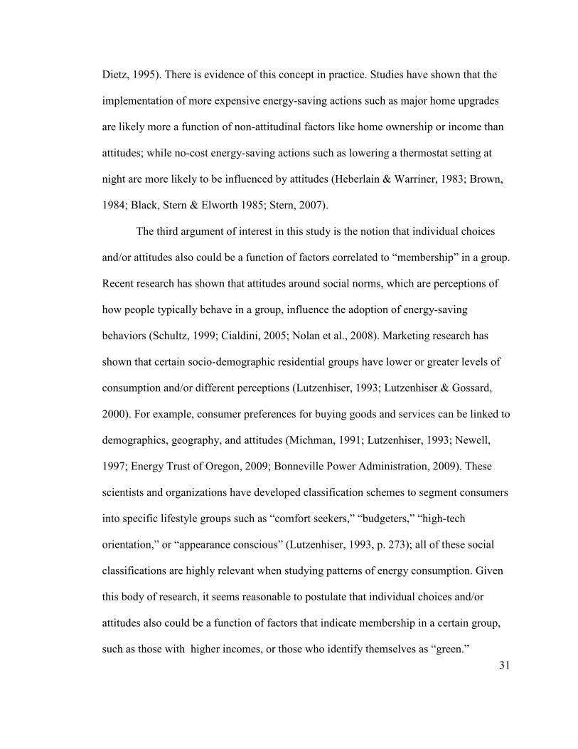
Figure 6: Relationships Between Missing Income Data and Outcome Variables ............ 46

Figure 7: Factors Influencing Energy Use Identified from the Literature Review ........... 53

Figure 8: Hypothesized Two-factor Structure (2002-2010 National Data) ...................... 62

Figure 9: Percentage of Cases Without Thermostat Access by Household Income ......... 67

Figure 10: Percentage of Cases Without Thermostat Access by Home Ownership ......... 67

Figure 11: Percentage of Cases Without Thermostat Access by House Type .................. 68

Figure 12: Percentage of Cases Reporting Thermostat-setting Behavior Among Those with Access to a Thermostat ............................................................................................. 69

Figure 13: Demographic and External Factors That Can Influence Energy-use Behavior Identified from the Literature Review .............................................................................. 77

Figure 14: CART Result (Pooled 2002-2006 National Data) ........................................... 84

Figure 15: Demographic and External Factors That Can Influence Energy-use Behavior Identified From the Literature Review ............................................................................. 93

Figure 16: Visualizing the Marginally Significant Interaction from Table 28 ............... 102

Figure 17: CART Result (Pooled 2004-2010 National Data) ......................................... 106

Figure 18: Hypothesized Two-factor Structure (2010 CA Data).................................... 113

Figure 19: Demographic and External Factors That Can Influence Energy-use Behavior Identified from the Literature Review ............................................................................ 119

Figure 20: Visualizing the Significant Interactions From Table 39 ............................... 127


xi

Figure 22: Visualizing the Significant Interactions from Table 40 ................................ 131


Figure 24: CART Result (2010 CA Data) ...................................................................... 133

Figure 25: PPIC Map of Political Ideology in California Across Counties .................... 136

1

1. INTRODUCTION

1.1 Larger Perspective

Household energy consumption and conservation have been topics of interest

among social scientists and policy makers for a number of decades. The energy crises of

the 1970s, which raised concerns about fossil fuel scarcity, were a major driver of federal

policy and research relating to energy efficiency and conservation (U.S. Congress, 1978).

Today, problems such as the impact of fossil fuel consumption on climate are the main

drivers of energy conservation research. In particular, energy production and

consumption (primarily involving fossil fuels) account for more than 80% of U.S.

greenhouse gas (GHG) emissions (U.S. Environmental Protection Agency, 2014). These

GHG emissions contribute to the greenhouse effect, which causes the Earth’s surface

temperature to rise. This also is called “global warming.”

The residential sector accounts for 22% of the total energy used in the U.S. (U.S.

Department of Energy, 2012). For this reason, this sector has been a target of various

energy efficiency and conservation programs implemented by utilities and federal, state,

or local governments. Utility funding for energy efficiency and related programs is the

main source of investment for energy efficiency and conservation in the residential

sector. From 2009 to 2013, the U.S. government invested an additional $16 billion in

energy efficiency through the American Recovery and Reinvestment Act (U.S. Congress,

2009; Goldman et al., 2010). The aim of these programs is to slow the rate of growth of

energy demand through investments in energy efficiency improvements in buildings and

related technologies.

2

However, addressing global warming requires greater reductions in energy

consumption than energy efficiency and conservation programs have been achieving.

States, including California, have developed ambitious goals for achieving “large net

reductions in energy use and emissions, rather than simply aiming to slow growth”

(Lutzenhiser, 2009, p. 1). To achieve these ambitious goals, a better understanding is

needed of how and why consumers invest or fail to invest in energy efficiency home

improvements or conservation tactics to reduce energy use.

This research is part of this broader ongoing effort that explores how consumers

make decisions around energy use in their homes. The focus is to assess whether certain

attitudes are associated with increased adoption of affordable and simple-to-perform

energy-saving actions. Specifically, this study explores a set of relationships between

environmental and other relevant attitudes and two energy-consumption choices:

thermostat-setting behavior and installation of energy-efficient lighting.

1.2 Research Objectives and Strategy

There are two main objectives in this study: (1) to examine attitude-behavior

patterns by using empirical data of household energy behavior choices, and (2) to

consider the value of different but salient theoretical notions about the effect of attitudes

on energy-saving choices.

The biennial Energy Conservation, Efficiency, and Demand Response Survey

(Abt SRBI & Research Into Action, 2002-2010) is the primary source of information for

characterizing the associations between attitudes and the selected energy-saving actions.

Researchers from Abt SRBI and Research Into Action implemented five waves of this

3

survey from 2002 to 2010, each occurring two years apart. In each wave, these

researchers used a random-digit-dial sample representative of the U.S. household

population. The survey questionnaire included items about attitudes and behaviors

regarding energy conservation and efficiency, motivations for saving energy, awareness

of ENERGY STAR®, and demographic characteristics. These survey data were combined

with state-level retail heating fuel price data, regional CFL price data, state-level heating-

degree-days (HDD), and state-level per capita funding for energy efficiency programs.1

These additional variables reflected the external conditions respondents were exposed to

at the time survey was conducted.

Analytically, this study primarily relied on the use of descriptive and inferential

statistical methods to assess the attitude-behavior relationships.

1.3 Organization of the Dissertation

Following this introductory section, Chapter 2 describes research questions,

relevant terminology, and reasons for researching this topic of interest. Chapter 3 presents

the literature review of energy consumption and conservation among U.S. households.

Chapter 4 provides an overview of the hypotheses being tested in this study. Chapter 5

contains the details of the research strategy, which includes descriptions of the datasets

and methodology. Chapters 6 and 7 present results from the analyses. Chapter 8

summarizes conclusions and implications from this study. Relevant supporting

information is documented in the appendices.

1 HDD measures the energy needed to heat a building.

4

2. RESEARCH OBJECTIVES AND QUESTIONS

2.1 Research Purpose and Knowledge Gaps

This study explores whether energy-related attitudes are associated with energy-

saving behaviors that are no- or low-cost and relatively simple to perform. From prior

research, there is evidence that attitudes around comfort, conservation, energy cost, and

social norms2 directly and indirectly influence a wide variety of household energy

consumption behaviors (see Section 3). There also is evidence that the attitudinal effect

on behavior is dependent on complexity and the cost of the behavior (see Section 3).

While this research is informative, there are still gaps in knowledge around this topic.

First, the majority of prior studies investigating the attitudinal effect on energy-

saving behavior occurred from the 1970s through the early 1990s (see Sections 3.1 – 3.3).

Not much is known about the attitudinal effect on energy-saving behavior after the 1990s.

Given this gap, this study explores the relationships between energy-related attitudes and

two affordable energy-saving behaviors based on studies that occurred from 2002 to

2010. Table 1 shows the two behaviors explored in this study.

2 Nolan et al. (2008) conducted two studies to assess whether descriptive norms impact household energy conservation behavior (see Section 3.2.4). They describe descriptive social norms as “how most people

behave in a given situation” (p. 913).

5

Table 1

Adoption of Selected Behaviors among U.S. Households (2002-2010 Survey Data)

Selected Behaviors 2002 2004 2006 2008 2010

Thermostat-Setting Behavior (i.e., a no-

cost, non-purchase behavior) n=697 n=568 n=623 n=801 n=800

Changed thermostat settings at various times of the day or night to save energy

(Only those with access to a thermostat) 84% 90% 89% No Data

No Data

CFL Installation (i.e., a low-cost

purchase behavior) n=900 n=798 n=798 n=801 n=800

Average number of CFLs in the home No Data 2.8 4.6 8.5 9.1

Second, there is a debate regarding how households make decisions to curb their

energy usage. Many social scientists argue that technical-economic assumptions, most

frequently used for predicting household energy consumption, do not sufficiently explain

the variability associated with energy consumption choices in the residential sector

(Lutzenhiser, 1993; Wilhite et al., 2000; Stern, 2007; Wilson & Dowlatabadi, 2007).

These social scientists posit that consumers’ energy consumption needs also are a

function of many noneconomic and nontechnical factors. This argument stems from

evidence that supports the power of cultural background, lifestyle, information uptake,

and a wide range of psychological variables to explain a significant amount of variation

associated with household energy consumption (Shipper et al., 1989; Hackett &

Lutzenhiser, 1991; Lutzenhiser, 1993; Guerin, Yust & Coopet, 2000; Abrahamse et al.,

2005; Stern, 2007; Wilson & Dowlatabadi, 2007). Given this debate, this study explores

how psychological factors, specifically attitudes, affect behavior by examining different

and salient theoretical notions about the effect of attitudes on energy-saving choices and

6

by using empirical data regarding household energy-behavior choices to learn more about

attitude-behavior relationships.

2.2 Terminology and Definitions

Terminology outlined in this section relates to behaviors and attitudes associated

with energy efficiency and conservation. This terminology specifies key conceptual ideas

at the core of this research.

There is a distinction between a conservation tactic to save energy (e.g., turning

off lights when not in use) and an energy efficiency investment (e.g., installing compact

fluorescent light bulbs or CFLs). Energy conservation tactics are actions associated with

“decreasing the use of existing capital equipment” (Black, Stern & Elworth, 1985, p. 5).

These actions rarely cost money and can result in a loss of amenity. An example of a

conservation tactic is manually changing thermostat settings throughout the day or night

in an effort to use less energy. Changing thermostat settings does not cost money, but it

can result in a loss of amenity if individuals must tolerate cooler or hotter indoor

temperatures by using less heat in the winter or less air-conditioning in the summer. In

contrast, energy efficiency investments are physical changes to the existing capital

equipment (Black, Stern, & Elworth, 1985, p. 5). These investments occur infrequently,

can be costly, and rarely result in a loss of amenity. For instance, one energy efficiency

action is replacing an older furnace with a newer and more efficient heating system. It is

costly to replace a furnace; nevertheless, replacing this system should not result in any

loss of amenity. This study focuses on thermostat-setting behavior (i.e., whether

respondents changed thermostat settings to save energy) and installation of CFLs.

7

Lowering (heating-related) or increasing (cooling-related) a thermostat setting is a

conservation tactic to save energy, whereas CFL installation is an energy efficiency

investment.

Attitudes are defined as “a psychological tendency that is expressed by evaluating

a particular entity with some degree of favor or disfavor” (Eagly & Chaiken, 1993, p. 1).

This definition implies that observable responses inferring the presence of an attitude are

those that express agreement or disagreement, liking or disliking, or similar reactions

about the object of evaluation. Many social scientists have categorized these evaluative

responses into three classes: affect, cognition, and behavior (Katz & Stotland, 1959;

Rosenberg & Hovland, 1960; Rajecki, 1982; Eagly & Chaiken, 1993). Affect denotes

positive or negative feelings about the object of evaluation (Eagly & Chaiken, 1993).

Thus, the affective component in an attitude is the evaluative element where the “attitude

holder judges the object to be good or bad” based on emotive reaction (Rajecki, 1982, p.

34). The cognitive component in an attitude refers to convictions insofar as one believes

that his or her opinions are correct (Rajecki, 1982). One can think of these convictions as

beliefs about the object of evaluation (Eagly & Chaiken, 1993). Finally, the behavioral

component in an attitude is the predisposition to act a certain way toward the object of

evaluation (Rajecki, 1982; Eagly & Chaiken, 1993). For example, an individual may say,

“I am too busy to be concerned about saving energy in my home.” This type of response

represents an intentional element in an attitude denoting one’s predisposition to act in a

certain manner.

It is not necessary to have all three of these components in place to capture an

attitude toward an object. For example, people can develop their attitudes about the

8

importance of conservation entirely by reading about it. In contrast, energy conservation

attitudes can also result from a mix of processes such as worrying about the cost of

energy, reading about the concept of peak oil, or having an ability to make one’s home

more energy-efficient.

This study will explore the connection between the selected behaviors and self-

reported attitudes toward the environment, cost of energy, and other factors that can

motivate people to reduce energy use at home, inferred from one’s beliefs, affect, or

intention.

2.3 Research Questions

Consumers have many options for curbing electricity or natural gas usage in their

residences. For example, they can install CFLs, add insulation, upgrade windows, install

more-efficient appliances, or adjust thermostat settings. Some of these behaviors do not

cost anything (i.e., non-purchase behaviors) and some are low- to high-cost purchase

behaviors. In this study, the thermostat-setting choice and installation of CFLs are studied

because these behaviors are no-cost or low-cost actions with the potential to reduce

residential energy use by 3-4% (see Table 2).

Table 2

Estimated Energy Savings Potential by Gardner et al. (2008)

Actions Estimated Percent of the U.S. Household

Energy Consumption Saved

1. Thermostat settings changed from 72°F to 68°F during

the day and set at 65°F at night for heating 3.4%

2. 85% of all [incandescent] light bulbs replaced with CFLs

4.0%

9

Since the focus of this study is to assess whether energy-related attitudes are

associated with the adoption of affordable and simple conservation and/or energy

efficiency actions, specifically thermostat-setting choice and CFL installation, the

following research questions have been formulated:

� What is the relationship between thermostat-setting choice and energy-related

attitudes?

� What is the relationship between CFL-installation behavior and energy-related

attitudes?

These research questions are examined by testing four hypotheses regarding how

these attitudes may relate to behaviors based on what is known and not known about

these relationships from prior research. The hypotheses are discussed in Chapter 4, after

the Literature Review Chapter.

10

3. LITERATURE REVIEW

Social scientists in various disciplines have been researching determinants of

household energy consumption in the U.S. since the energy crises of the 1970s. This

energy-related research provides useful information about how consumers make energy

efficiency and conservation choices. This chapter describes and reviews that literature.

The following topics are covered: (1) determinants of household energy consumption and

curtailment choices, (2) the role of attitudes in decision making around energy use, and

(3) theoretical approaches for investigating the impact of attitudes on residential energy

demand.

3.1 Household Energy Consumption and Conservation

This section examines the most notable determinants of household energy

consumption and conservation, including physical house attributes, occupant

characteristics, climate conditions, energy efficiency policies, and energy prices.

3.1.1 Determinants of Electricity and Natural Gas Consumption

Household demand for energy is dependent on the physical attributes of a home

and weather (Socolow et al., 1978; U.S. Department of Energy, 2009). In nine identical

townhouses studied by Socolow et al., 35% of winter energy loss was due to improperly

insulated attics despite the presence of nine centimeters of fiberglass insulation. Retrofits

of the townhouses (addition of attic insulation and air sealing of walls, doors, and

windows) reduced overall energy consumption for space heating by 15-30%. Many other

11

studies, reviewed by Guerin, Yust, and Coopet (2000) and Berry and Schweitzer (2003),

confirmed that weatherizing a home could decrease a demand for energy in winter and

summer months.

Another notable finding from the Socolow et al. study (1978) was that the new

occupants in the same house had energy consumption levels nearly unrelated to the

consumption levels of the previous occupants. A further investigation revealed that 33%

of the variance associated with energy use in that study was explained by the occupants’

behavior (Sonderegger, 1978). Other research has shown that the most common occupant

characteristics notably affecting household energy consumption are household income,

occupants’ age, household size, and willingness to weatherize a home (see Figure 1).

Figure 1: Occupant Determinants of Household Energy Consumption

Use Less Energy Use More Energy

Those with low incomes (This pattern is striking when energy prices rise.)

Those with higher incomes

Those who are younger, without children, or live in smaller families/households

Those who are older, with children, or live in larger families/households

Those who had weatherized their home and/or invested in other energy home

improvements

Those who had not weatherized their home or invested in other energy

home improvements

Sources: Hackett and Lutzenhiser (1991); Poyer, Henderson and Teotia (1997); Guerin, Yust and Coopet (2000); O’Neill and Chen (2002); Berry and Schweitzer

(2003); and Lutzenhiser and Bender (2008).

Social scientists also have found that broader societal conditions influence energy

consumption in the residential sector. Wilhite et al. (2000) provided ample evidence that

household energy consumption was conditioned by the “upstream systems” (p. 114) that

have been constructed to serve the needs of a society, such as housing designs or product

designs. Appliance industry standards are one kind of “upstream system.” Mandated

12

changes in these standards, specifically stipulations about the energy efficiency of various

product designs, have effected significant energy savings for individuals and the nation as

a whole (Gillingham, Newell & Palmer, 2006).

Another set of social conditions that influence residential energy demand is

existence of institutional market interventions promoting energy efficiency. For example,

in 1983 the Bonneville Power Administration (BPA) began encouraging homebuilders in

the Pacific Northwest to adopt Model Conservation Standards (MCS) by providing

financial incentives and technical assistance to local governments that promoted these

standards (Geller & Nadel, 1994).3 In 1986, regional utilities created a program

supporting adoption of the MCS through training and assistance to homebuilders. By

1988, homebuilders had constructed 7,000 homes according to the MCS; this represented

17% of the new housing stock at that time (Geller & Nadel, 1994). The adoption of the

MCS through this institutional intervention had a profound effect on residential energy

consumption in the Northwest. BPA demonstrated that houses constructed according to

the MCS used 42-45% less energy than a control group of non-MCS homes – a

substantial energy savings (Geller & Nadel, 1994, p. 325).

However, not all social interventions result in notable residential energy savings.

In the U.S., utility-managed institutional interventions often use informational,

educational, and financial tactics to achieve energy efficiency gains in the residential

3 Prior to 1983, homes in the Pacific Northwest were constructed with single-pane windows and modest levels of insulation. To improve the energy efficiency of new homes at that time, the Northwest Power Planning and Conservation Council developed Model Conservation Standards (MCS) by recommending “reduced window area; improved thermal resistance of windows, walls, and roofs; and reduced air

infiltration” (Geller and Nadel, 1994, p. 324).

13

sector (Geller & Nadel, 1994; Lutzenhiser et al., 2009). Research has shown that these

tactics are not always effective at encouraging households to reduce energy consumption.

Abrahamse et al. (2005) reviewed thirty-eight studies on this topic within the field of

social and environmental psychology. These researchers identified three prominent

patterns: (1) Information received by households on energy efficiency and conservation

resulted in more knowledge of these matters but not in behavioral change; (2) Monetary

rewards, such as rebates, were successful in encouraging energy conservation among

households, but they had short-term effects; and (3) Frequent energy consumption

feedback given to households reduced energy consumption by high-energy-using

households but not necessarily by low-energy-using households.

Presently, the price effects of electricity, natural gas, or other fuels on residential

demand for energy are small. In 2003, long-term price elasticity was estimated at 0.49 for

electricity, 0.41 for natural gas, and 0.60 for distillate fuel for the residential sector in the

U.S. (Wade, 2003; estimates are given as absolute values).4 From 1984 to 2003, short-

term price elasticity for residential customers across 19 states was between 0.14 and 0.44

for electricity, 0.03 and 0.76 for natural gas, and 0.15 and 0.34 for distillate fuel

(Gillingham, Newell & Palmer, 2009, p. 6; estimates are given as absolute numbers).

These estimates, which are ratios of the percent change in price compared to the percent

4 Price elasticity of demand is a measure used in economics to show any impact of price change on demand for a product or service. It is reported as a percent change in quantity demanded divided by the percent change in price. If price elasticity is less than one, a percent change in price results in a smaller percent change of quantity demanded relative to the percent change of quantity demanded when a price elasticity is

greater than one.

14

change in energy demanded, indicated that changes in the price of energy were not

notably changing the demand for energy.

Nevertheless, there is evidence that substantial increases in the price of energy

can substantially influence energy consumption in the residential sector. During the

California energy crises of 2000 and 2001, a rapid increase of the price of electricity

reduced household energy consumption in the City of San Diego by an average of 13%

over a period of 60 days (Reiss & White, 2008).5 Reiss and White also found that this

decline in consumption stopped as soon as electricity prices stabilized due to an imposed

price cap. This study indicates that consumers can reduce their energy consumption

quickly if they experience rapid increases in the price of energy.

From this body of research, it is evident that household energy demand is a

function of these conditions: building attributes, occupant characteristics and behaviors,

and external conditions (including weather, policies, and energy prices).

3.1.2 Determinants of Energy Efficiency and Conservation Behaviors

For consumers to reduce their energy use at home, they must either adopt energy-

conservation tactics (e.g., lowering the thermostat setting on a water heater) or invest in

energy home improvements (e.g., upgrading attic insulation). Across numerous research

studies, the most frequently observed factors significantly affecting households’ energy

conservation or efficiency behaviors were socio-demographic and attitudinal variables,

such as home ownership, age, attitudes around comfort, conservation, energy costs and

5 California had a shortage of electricity in 2000 and 2001.

15

social norms, and feedback interventions about electric or natural gas usage in a home

(see Figure 2).

Figure 2: Determinants of Energy Efficiency or Conservation Behavior

Use conservation tactics to

save energy

Invest in energy-efficient

home upgrades

Those who are younger and without

young children Those with higher incomes

Those who are more willing to tolerate

cooler/hotter temperatures in a home Home owners

Those who receive frequent feedback

on energy usage

Those who value the personal benefits of the investment (e.g.,

improved comfort, health, and/or

home value)

Those who worry about energy costs

and want to reduce them Presence of a home handy-person

Those who believe in the importance

of conservation

Those who feel socially pressured to conserve or guilty about not

conserving

Sources: Stern et al. (1986); Peters (1989); Guerin, Yust and Coopet (2000);

Abrahamse et al. (2005); and Stern (2007).

Further assessment of these relationships indicates that the landscape of

household energy consumption is highly complex. Specifically, there are three major

areas of complexity in perceiving consumers’ adoption of energy-saving behaviors. First,

as early as the 1980s, Black, Stern, and Elworth (1985) recognized that various

socioeconomic, attitudinal, and physical factors were associated with different energy-

saving behaviors. In this study of 478 Massachusetts residents, home ownership had the

greatest influence on major energy efficiency capital investments, while income had an

indirect effect, mainly through home ownership. Personal norms such as “…sense of

16

personal obligation and pride with respect to insulating the home and getting the same

comfort for less energy” (p. 9), had the greatest effect on low-cost efficiency

improvements, such as sealing cracks around doors or windows or weather-stripping.

These findings demonstrated that the effects of socio-economic and psychological factors

depend on the type of behavior.

Second, numerous economic and psychological concerns hinder consumers’

willingness to conserve energy. This is particularly evident in behaviors specific to

energy efficiency home improvements. Prior research indicated that energy costs as a

proportion of total expenditures, transaction costs of information gathering, tendency to

be risk-averse, heterogeneity of preferences, lack of information, lack of trust in

information sources, and adverse reactions to physical home changes explain a lack of

investment in cost-effective energy efficiency home upgrades (Lutzenhiser, 1993;

Frederick, Loewenstein & O'Donoghue, 2002; Wilson & Dowlatabadi, 2007). Generally,

consumers tend to place a higher weight on information that is psychologically vivid and

observable (Yates & Aronson, 1983). For example, households are sensitive to the initial

costs of energy-efficient home upgrades and they often use current energy prices to

calculate the payback for these capital investments (Gillingham, Newell & Palmer, 2009).

This is problematic for two reasons: (1) Households that are worried about initial costs

likely will downplay the long-term benefits of investing in energy efficiency home

improvements; and (2) Households that base estimated energy savings on current energy

prices, without factoring in likely price increases may erroneously conclude that the

investment is not worth making.

17

In addition, variability in consumers’ demand for energy is related to their

willingness to save energy. An energy user initiates energy consumption through various

physical devices for the purposes of obtaining specific services (Wilhite et al., 2000).

Thus, demand for energy is indirect and driven by the type of service a user desires, such

as comfort, cleanliness, or entertainment. This need for various services is associated

with consumers’ lifestyles – the way people live (Shipper et al., 1989; Lutzenhiser &

Gossard, 2000; Wilhite et al., 2000). Marketing researchers have shown that consumers’

preferences for goods and services can be linked to demographics, geography, and

attitudes (Michman, 1991; Newell, 1997). These scientists have developed classification

schemes to segment consumers into specific lifestyle groups such as “comfort seekers,”

“budgeters,” “high-tech orientation,” or “appearance-conscious” (Lutzenhiser, 1993, p.

273). All of these social classifications are highly relevant when studying patterns of

energy consumption.

Further research has shown that specific lifestyles are associated with lower or

higher levels of consumption (Lutzenhiser & Gossard, 2000). For example, individuals

who value thermal comfort were less willing to adjust thermostat settings in order to save

energy (Seligman et al., 1979; Becker et al., 1981). Yet, Keirstead’s (2005) review of the

literature from 1980s to 2005 presents strong evidence that the sociological,

anthropological, marketing, and interdisciplinary studies most likely to conduct this type

of research declined sharply after 1990. This is important to note because it indicates that

newer research is needed to assess the link between lifestyle choices and energy use.

18

3.2 Attitudes and Energy Conservation

3.2.1 Attitude Formation

An individual acquires attitudes from parents (Sinclair, Dunn & Lowery, 2005),

peers (Poteat, 2007), the media (Hargreaves & Tiggemann, 2003), and many other

sources. Many competing theories explain attitude formation, of which these three are the

most notable: Cognitive Dissonance Theory (Festinger, 1957), Elaboration Likelihood

Model (Petty & Cacioppo, 1979, 1986), and Theories of Learning (Pavlov, 1927;

Skinner, 1938; Bandura, 1977).

Festinger's Cognitive Dissonance Theory describes a mechanism of how

perceptions, including attitudes, are acquired and changed. This theory posits that people

want to have consistent perceptions and behaviors. Mismatch between perceptions and

behaviors will lead to inner conflict (i.e., cognitive dissonance). Because people want to

avoid inner conflict, they are willing to change their behavior or perception to ensure

their behavior aligns with their perception.

The Elaboration Likelihood Model describes another mechanism of how attitudes

could be acquired and changed. This model suggests that individuals can be persuaded to

form a new attitude. This can occur in two ways:

� First, people are willing to listen to a message and think about the merit of that

message. This cognitive process will lead to an attitude shift if the message is deemed

persuasive – that is, people will believe the message and develop an attitude around it,

if they find it convincing.

19

� Second, people are influenced by the characteristics of the speaker delivering the

message or by the contextual cues not associated with the merit of the message. These

cues can lead to change in attitudes for those who use the cues to determine the

credibility of the message. However, any attitudinal changes based on cues rather

than the message itself often are temporary (Petty & Cacioppo, 1979, 1986).

Finally, learning is an important aspect of attitude formation. Theories of

Learning attempt to describe how people learn. Among these, social learning (Bandura,

1977), classical conditioning (Pavlov, 1927), and operant conditioning (Skinner, 1938,

1957) provide some important insights into how attitudes are acquired. Social learning is

learning by observing others. For example, when someone you admire and respect has a

particular attitude, you are more likely to develop the same attitude. Classical

conditioning refers to a process whereby a person develops a positive or negative

association about a neutral object when that object is paired with a positive or negative

stimulus. For instance, a person can develop a positive attitude toward a dress when that

dress is paired with an attractive model. Operant conditioning refers to a process of

changing a behavior by using positive or negative reinforcement after the desired

response. For example, if a man expresses a positive attitude about dogs and receives a

positive response from others about that attitude, that attitude will be reinforced and will

get stronger.

20

3.2.2 Attitude Function

Researchers have tried to assess why individuals hold attitudes. The prevailing

theory on this matter is Katz’s (1960) Functionalist Theory. This theory posits that

attitudes form to serve many functions, of which these four are the most notable:

� Utilitarian function (i.e., an individual develops attitudes that are rewarding to

avoid punishment)

� Knowledge function (i.e., an individual develops attitudes to organize and

understand information in a meaningful way)

� Ego-defensive function (i.e., an individual develops attitudes to help protect his/

her self-esteem)

� Value-expressive function (i.e., an individual develops attitudes to express central

values or beliefs)

3.2.3 Attitude-Behavior Connection

In this study, attitudes are defined as “a psychological tendency that is expressed

by evaluating a particular entity with some degree of favor or disfavor” (Eagly &

Chaiken, 1993, p. 1). Prior psychological research, from 1930s to 1960s, did not provide

conclusive evidence that attitudes were good predictors of behaviors (see review by

Eagly & Chaiken, 1993, Ch.4). Thus, social psychologists began to question the notion

that attitudes can predict behavior, and by 1970, theories such as Festinger’s (1957)

Cognitive Dissonance Theory, which indicates that behaviors may change attitudes,

became quite popular. In light of this, a number of social psychologists began to claim

that attitudes were poor predictors of behavior. This became a controversial issue and

21

stimulated new research on the attitude-behavior relationship after the 1960s. This newer

research provided evidence that attitudes can moderately predict behavior under certain

conditions. This section presents this empirical research and its importance to this study.

Seminal work by Fishbein and Ajzen (1975) and Ajzen (1991) presented a line of

evidence showing that attitudes can be in a causal role in relation to behavior. These

researchers asserted that attitudes (cognitive beliefs), in conjunction with subjective

norms (beliefs of those who are important to the individual), predict volitional behavior

through behavioral intention. This is known as the Theory of Reasoned Action. This

theory had been tested in many studies and was successful in explaining blood donation

(Pomazal & Jaccard, 1976), voting (Ajzen & Fishbein, 1980; Fishbein et al., 1986), and

purchases of various consumer products (Brinberg & Cummings, 1983). In an extensive

meta-analysis of 113 articles exploring this relationship as hypothesized by the Theory of

Reasoned Action, Van den Putte (1991) observed that the mean R for predicting

behavioral intention from attitudes and subjective norms was 0.68, and the mean R for

predicting behavior from behavioral intention was 0.62. This provided evidence that

attitudes can affect how consumers behave.

Further examination indicated that the Theory of Reasoned Action was successful

in explaining simple volitional behavior such as voting but not the behaviors that require

“skills, abilities, opportunities, and the cooperation of others” (Liska, 1984, p. 63). Thus,

Ajzen (1991) expanded the Theory of Reasoned Action to include behavioral constraints

in the model. This newer theory, titled Theory of Planned Behavior, states that one’s

intention to engage in a behavior depends on the amount of control one has over this

behavior. For example, renters cannot readily make changes to their homes since they do

22

not own the property. In the area of energy conservation, the likelihood of adopting an

energy-conservation and/or energy efficiency action depends on factors such as home

ownership, finances, or the life cycle stage of members of the household (see Section

3.1.2). For this reason, it is important to consider situational conditions in assessing the

attitudinal effect on energy behavior.

Studies in laboratory settings have emphasized the importance of context when

thinking about attitudinal effect on behavior (Snyder & Swann, 1976; Millar & Tesser,

1986). For example, prior knowledge about an object moderates the effect of attitudes on

behavior (Fazio & Zanna, 1981; Davidson et al., 1985; Kallgren & Wood, 1986) and past

behavioral experiences correlate moderately with attitudes and their effect on behavior

(Regan & Fazio, 1977; Fazio & Zanna, 1981). Snyder and Kendzierski (1982) and

Borgida and Campbell (1982) showed that relevant attitudes influence behavior directly

in those situations where situational variables have a weak effect on the behavior. This

body of literature indicates that it is challenging to explore the attitudinal effect on

behavior, as the effect can depend on many factors within the context of the study.

3.2.4 Attitudes and Energy Behavior Research

In the 1980s, research showed that attitudes toward comfort and attitudes toward

conservation can explain a significant amount of variation of self-reported thermostat

setback choices (Seligman et al., 1979; Beck, Doctors & Hammond, 1980; Becker et al.,

1981; Brown, 1984; Hand, 1986). Households that used more energy were less willing to

tolerate cooler or hotter temperatures inside their home during winter or summer

(Seligman et al., 1979; Becker et al., 1981). In contrast, residents with pro-conservation

23

attitudes were more likely to lower their thermostat settings when heating their homes

than residents without such attitudes (Beck, Doctors & Hammond, 1980). Peters (1989)

revealed that concerns for comfort had a stronger influence on conservation behavior than

conservation attitudes. Black, Stern, and Elworth (1985) noticed that attitudes toward

conservation had the greatest effect on the adoption of inexpensive energy efficiency

choices.

In addition to these findings, recent studies have shown that attitudes related to

descriptive social norms influence the adoption of energy-saving behaviors (Schultz,

1999; Cialdini, 2005; Nolan et al., 2008). Descriptive social norms are people’s beliefs of

what is commonly done in a group or a situation. Nolan and colleagues (2008) reported a

notable effect between descriptive social norms and conservation behaviors. They

interviewed 810 respondents in California and measured their motivations for conserving

energy. The top reason to conserve was “environmental protection,” followed by

“benefits to the society,” “saving money,” and “other people are doing it.” A follow-up

analysis of these data revealed that among those four reasons to conserve, the strongest

predictor of actual conservation behavior was the one mentioned least frequently ˗˗

“other people are doing it.” Specifically, in a field study of households from San Marcos,

California, they found that those who received and saw door messages containing “others

are doing it” script saved significantly more energy than participants who saw messages

containing statements such as “it is good for the environment,” “it saves money,” and “it

is beneficial for the society.”

A further assessment of attitude-behavior relationships revealed that attitudes

influence the adoption of various conservation behaviors in conjunction with other

24

factors. Lutzenhiser (1993) concluded that attitudinal effects on a behavior were

dependent on the complexity and cost of that behavior. He found that models considering

the effect of attitudes and constraints – constraints relevant to cost and the complexity of

the action–better predicted the adoption of conservation actions than models exploring

the attitudinal effect only. Stern (2007) found that the strongest predictors of energy

efficiency and conservation choices were available technology, physical features of a

home, social norms and expectations, material costs, returns on investment, and

convenience. Personal capabilities, habit, and attitudinal factors still mattered, but the

effect of these variables on energy consumption was often indirect and specific to the

behavior in question (Stern, 2007). Wilson and Dowlatabadi (2007), the authors of the

most recent review on decision making associated with residential energy use, recognized

that energy-saving behaviors relate to psychosocial characteristics, such as perceived

costs and house amenity losses. Given this research, it is likely that attitudinal effects on

a behavior are dependent on cost, psychosocial characteristics, and other situational

variables.

3.3 Current Theoretical Perspectives of Energy Consumption Choices

This study explores the attitude-behavior associations from different but related

theoretical lenses. The aim is to better understand how attitudes and contextual factors

inter-relate and affect behavior. The following sections present relevant theoretical

perspectives from the field of economics, social psychology, and sociology for explaining

energy consumption in the residential sector.

25

3.3.1 The Most Frequently Used Framework for Estimating Energy Use

The most commonly utilized theoretical framework for estimating household

energy consumption is the Physical-Technical-Economic Model (PTEM) (Lutzenhiser,

1993; Wilhite et al., 2000; Lutzenhiser et al., 2009). This model uses physical

characteristics of buildings and/or appliances, prices of energy or higher-efficiency

goods, and behavioral assumptions about the use of equipment inside a residence to

predict patterns of consumption in the residential sector.

A specific example of this type of model is Conditional Demand Analysis (CDA).

In 1980, Parti and Parti developed the CDA framework to estimate electricity demand for

heating, cooling, and related uses across the population of households in the City of San

Diego. These researchers employed regression equations to disaggregate household

monthly billing data into heating or other energy needs by using relevant thermodynamic

and behavioral relationships. For example, a regression model of energy consumption for

heating would be a function of weather, type and size of a dwelling, heat source (e.g.

electricity or natural gas), and any behaviors associated with heating. Their model

explained a fair amount of variability in monthly billing data; R² values ranged from 0.58

to 0.65. Considering such relatively high R² values, energy analysts found this model

promising for predicting energy demand of various end uses (Swan & Ugursal, 2009).

Energy analysts using the PTEM perspective, such as in the CDA model, assume

that behaviors determining energy consumption in a home can be explained by the

traditional economic rationale (Swan & Ugursal, 2009). This rationale suggests that

energy users view energy as an input that allows them to obtain goods through which

they receive “utility” (i.e., pleasure or satisfaction). In particular, energy users will

26

choose a good that allows them to maximize their utility, while minimizing the cost.

Thus, consumers investing in energy efficiency home upgrades, for example, analyze

such purchases in terms of their budget and preferences and consider all options. This

utility-specific economic perspective can be described as:

Da = f (Pa, Pb, I, Cp)

Where Da is a demand for a good “a”; Pa is a price of good “a”; Pb is a price of other

similar goods; I is income; and Cp is the consumer’s preference for good “a” (derived

from Boardman et al., 2006, p. 31 and McConnell & Brue 2005, p. 376).

Empirically, research has shown that demand for energy depends on consumer

preferences for goods or services, income, and price (Kristom, 2008). For example,

households responding to an energy price increase can change thermostat settings, add

insulation, or move to a more energy-efficient house to reduce the percentage of their

budget they spend on energy. Thus, preferences in conservation choices can vary in the

short and long run. Changing thermostat setting is a short-run behavior, while moving to

a more energy-efficient home is a long-run behavior. A meta-analysis of 36 studies on

residential electricity demand between 1947 and 1997, suggests that short-run income

elasticity is approximately 0.28 and long-run income elasticity is approximately 0.97

(Espey & Espey, 2004). This implies that increases in income have a more notable effect

on the demand for energy in the long run rather than the short run. However, both income

and price elasticity of energy demand are not constant; they can change over time and for

certain types of consumers (Dubin & McFadden, 1984; Lutzenhiser, 2002; Kristom,

2008).

27

3.3.2 Limitations of the PTEM Perspective

Prominent social scientists who study energy consumption (Lutzenhiser, 1993;

Wilhite et al., 2000; Stern, 2007) and Wilson and Dowlatabadi (2007), assert that PTEM

is insufficient in explaining all behavioral patterns of consumption. They state that PTEM

lacks psychological and social variables that are highly relevant for predicting such

patterns. Hence, estimates of energy demand based on the PTEM perspective could be

improved if relevant non-technical and non-economic variables are included in the

model. This section explores the value of these claims.

Research has shown that PTEM models result in erroneous estimates of energy

demand. An example of this was the CDA energy demand statistic for central air-

conditioning in two regions in California (U.S. Department of Energy, 1996). This

estimate from the 1990 Residential Energy Consumption Survey (RECS)6 database was

33% to 370% higher in two utility service territories in California than the same air-

conditioning estimate from the sub-metered studies – studies that directly metered energy

use from a set of appliances. This finding indicated that the CDA model failed to

accurately predict energy demand for air-conditioning.

In addition, consumers fail to consider all the alternatives when buying more-

efficient products, exhibit difficulties in computing the rate of return on their investment,

lack important information about energy-efficient products and services, and choose

6 The Residential Energy Consumption Survey (RECS) has collected information about the use of energy

across U.S. households every four years since 1987.

28

options that are not optimal in the long run (Lutzenhiser, 1993; Stern, 2007; Wilson &

Dowlatabadi, 2007). These findings are important to recognize since they suggest that

consumers are not the rational thinkers traditional utility economic models assume them

to be. This is not surprising since seminal work by Tversky and Kahneman (1981) and

Simon (1957, 1987) demonstrated that people make different choices when a statistic

about a situation is framed as a loss rather than a gain. In particular, these researchers

found that people are sensitive to losses and do not always seek the option that will be

best for them over time. Instead, individuals base their decisions on a “rule” they believe

in. These findings have been replicated in more recent economic literature (Wilson &

Dowlatabadi, 2007). As a result, social scientists who criticize the PTEM perspective

(which uses the traditional utility model of consumer choice) recommend using an

integrative approach to explain energy consumption. Such an integrative approach would

combine relevant knowledge from social psychology, sociology, and economics to

determine the decision-making mechanisms that underlie people’s consumption choices.

Unfortunately, Keirstead’s (2006) review revealed that consumer behavior models

integrating economic-technical assumptions with psychological or sociological notions of

consumer choice are rare. Keirstead found two significant patterns in the literature: (1)

Household energy interdisciplinary research in the U.S. declined sharply in the last two

decades; and (2) Economic and engineering studies were significantly more present in

this literature than any other kinds of studies. Keirstad stated that there is a need for

further research of interdisciplinary perspectives in this realm.

29

3.3.3 Relevant Theoretical Perspectives Explaining the Attitude-Behavior Link

In economics, social psychology, and sociology, related but different attitude-

behavior hypotheses exist that are relevant for studying energy efficiency or conservation

behavior. These hypotheses are components of larger theories that describe how personal

variables such as attitudes and external or contextual factors interrelate and affect

behavior. Three such arguments are of interest in this study.

The first argument comes from the traditional economic perspective, which treats

consumer behavior as a function of individual preferences and budget. Essentially, there

is an optimal level of consumption (shown in Figure 3). It is the point at which

consumers obtain the greatest utility given their budget. Prior econometric research

provided some evidence of this type of behavior; economists found that households

changed their consumption patterns after making their homes more energy-efficient

(Hirst, White & Goeltz, 1985; Dubin, Miedema & Chandran, 1986). In particular,

households increased their level of energy consumption after a home retrofit, which

eroded some of the expected energy savings gains from these retrofits. Although, Hirst,

White, and Goeltz (1985) found that 13% of electric savings for space heating was lost

due to an increase of 0.8°F in indoor temperatures after the retrofits, this effect likely was

small in absolute terms. Peters (1989) noticed that “in the Willamette Valley (in Oregon;

some of the households in Hirst, White, and Goeltz [1985] study lived in this region),

with approximately 4,000 Degree Days per year, 1°F reduction in winter indoor

temperature will result in a 4% savings in energy consumption” (p. 2). The Hirst, White,

and Goeltz study did show that consumers have different preferences for using energy

30

when costs change – i.e. since they could afford more of it, they opted to use more of it

even if “more” was relatively small in absolute terms. This comports with the economic

concept that costs and income (a proxy for a budget), and preferences (such as attitudes)

affect consumption.

Figure 3: Indifference Curves Adapted from McConnell and Brue (2005, p. 386-391)

A second argument explored in this study is Stern’s (2007) claim that the effect of

personal variables, such as attitudes, on a behavior is dependent on contextual or

situational variables, such as the availability of a new technology, the financial cost of

adopting a behavior, and other such factors (p. 374, conclusion #4). Stern asserts that

“The strength of psychological influences varies from moderate to weak to almost

nonexistent, dependent on the strength of non-psychological factors…” (p. 374-375).

This claim is a variation of the Attitude-Behavior-External Condition Model. According

to this model, attitudes lead to behavioral change in those contexts where an individual is

not constrained by cost, technology, or any other external factors (Guagnano, Stern &

31

Dietz, 1995). There is evidence of this concept in practice. Studies have shown that the

implementation of more expensive energy-saving actions such as major home upgrades

are likely more a function of non-attitudinal factors like home ownership or income than

attitudes; while no-cost energy-saving actions such as lowering a thermostat setting at

night are more likely to be influenced by attitudes (Heberlain & Warriner, 1983; Brown,

1984; Black, Stern & Elworth 1985; Stern, 2007).

The third argument of interest in this study is the notion that individual choices

and/or attitudes also could be a function of factors correlated to “membership” in a group.

Recent research has shown that attitudes around social norms, which are perceptions of

how people typically behave in a group, influence the adoption of energy-saving

behaviors (Schultz, 1999; Cialdini, 2005; Nolan et al., 2008). Marketing research has

shown that certain socio-demographic residential groups have lower or greater levels of

consumption and/or different perceptions (Lutzenhiser, 1993; Lutzenhiser & Gossard,

2000). For example, consumer preferences for buying goods and services can be linked to

demographics, geography, and attitudes (Michman, 1991; Lutzenhiser, 1993; Newell,

1997; Energy Trust of Oregon, 2009; Bonneville Power Administration, 2009). These

scientists and organizations have developed classification schemes to segment consumers

into specific lifestyle groups such as “comfort seekers,” “budgeters,” “high-tech

orientation,” or “appearance conscious” (Lutzenhiser, 1993, p. 273); all of these social

classifications are highly relevant when studying patterns of energy consumption. Given

this body of research, it seems reasonable to postulate that individual choices and/or

attitudes also could be a function of factors that indicate membership in a certain group,

such as those with higher incomes, or those who identify themselves as “green.”

32

This study explores these related and distinct ideas of how attitudes can affect

behavior by using empirical data regarding household energy behavior choices to learn

more about attitude-behavior relationships from those data.

3.4 Conceptual Framework for This Study

Two important insights emerged from the research presented in this chapter. First,

many factors affect residential energy consumption behavior (see Figure 4).

Figure 4: Factors Influencing Energy-use Behavior

Sources: Research noted in Sections 3.1 and 3.2.

Second, complex relationships exist between these determinants of energy use

and behavior (see Section 3.2). Specifically, energy-related attitudes can directly affect

behavior, if there are no constraints (e.g., low income). If there are constraints, the

attitudinal effect on behavior will be either indirect or dependent on the constraining

variables (Ajzen, 1991; Lutzenhiser, 1993; Stern, 2007), as illustrated in Figure 5. The

body of research discussed in the preceding sections shows that factors such as home

ownership, finances, pertinent knowledge, or the life cycle stage of members of a

household often affect attitude-behavior relationships.

Individual

Perceptions (including attitudes) about:

conservation, comfort, social norms, and perceived costs

Age

Pertinent Knowledge

Environment

Structure

House size, age

R-value of insulation

Equipment type (appliances, HVAC, etc.)

ExternalWeather

Energy prices

Energy efficiency programs

Building codes

Appliance standards

HouseholdsAges (young,

elderly)

Home owners

Someone handy at home

Income

# of occupants

33

Figure 5: Possible Attitude-Behavior Relationships

Direct Indirect Dependent

This study examines whether relationships between energy-related attitudes and

behavior are direct or dependent on other factors, while controlling, to the extent

possible, for important situational and external factors listed in Figure 4. Three theoretical

viewpoints of how attitudes may relate to behavior, described in Section 3.3.3, serve as a

conceptual roadmap for how attitudes and contextual factors may inter-relate either

directly or through a moderator variable to affect behavior. The goal is to learn more

about the associations between energy behaviors and attitudes by exploring plausible

relationships between attitudes and behaviors suggested by the theoretical viewpoints

referenced in Section 3.3.3. Attitude formation is not examined in this study due to lack

of data.

Attitudes Behavior Attitudes Intervening Variable Behavior Attitudes

Moderator Variable

Behavior

34

4. STUDY HYPOTHESES

As noted in Section 2.3, this study focuses on these two research questions:

� What is the relationship between thermostat-setting choice and energy-related

attitudes?

� What is the relationship between CFL installation behavior and energy-related

attitudes?

To address these questions, this study examines four specific hypotheses related to how

these attitudes may correspond to behaviors, based on what is known and not known

about these relationships from prior research.

The majority of previous studies investigating the attitudinal effect on energy-

saving behavior originated between the 1970s and early 1990s. From these studies, it is

known that attitudes toward comfort and conservation can explain a significant amount of

variation of self-reported thermostat setback choices (Seligman et al., 1979; Beck,

Doctors & Hammond, 1980; Becker et al., 1981; Brown, 1984; Hand, 1986; Peters,

1989). Black, Stern, and Elworth (1985) also noticed that attitudes toward conservation

had the greatest positive effect on the adoption of inexpensive energy efficiency choices.

Since this research has expanded little since the mid-1990s, there is a need to examine

whether similar attitude-behavior relationships still occur.

� Hypothesis 1: Energy attitudes explored in this study are positively associated

with the thermostat-setting behavior (i.e., changing the thermostat setting to save

energy) and CFL installation behavior.

35

More recent research has shown that certain energy-related attitudes in the U.S.

are changing, and not necessarily in the same direction (Bolsen & Cook, 2008; Saad,

2013). For example, general public opinion polls show that Americans' self-reported

concern about global warming peaked in 2000, declined from 2001 to 2005, peaked again

between 2006 and 2008, and declined again between 2009 and 2010 (Saad, 2013).

Similarly, the polls show that Americans' self-reported concern about the U.S. energy

situation peaked in the 1970s, declined in the 1990s, and peaked again in the recent years.

These findings suggest that energy-related attitudes change over time. If that is accurate,

this may lead to an inconsistent attitudinal effect on a behavior over time.

� Hypothesis 2: The attitude-behavior relationships explored in this study do not

persist over time (i.e., from 2002 to 2010).

Prior studies also have shown that implementation of more expensive energy-

saving actions, such as major home upgrades, are more likely a function of non-

attitudinal factors like home ownership or income than attitudes; whereas, no-cost

energy-saving actions like lowering a thermostat setting at night are more likely to be

influenced by attitudes (Heberlain & Warriner, 1983; Brown, 1984; Black, Stern &

Elworth, 1985). This research supports the traditional economic perspective of how

consumers make choices (i.e., consumer choice is a function of budget), and Stern’s

(2007) claim that an attitudinal effect on a behavior increases when an individual is not

constrained by cost or any other situational factors.

� Hypothesis 3: Household budget moderates attitude-behavior relationships

explored in this study (an economic perspective). Household budget will have a

greater influence on the attitude-behavior relationship when the behavior is the

36

purchase of an energy-efficient product rather than a no-cost conservation action

(inferred from Stern's social psychology perspective).

Finally, research has demonstrated that different socio-demographic groups have

lower or greater levels of energy consumption and different attitudinal characteristics

(Lutzenhiser, 1993; Lutzenhiser & Gossard, 2000; Stern, 2007). This research suggests

that individual choices and/or attitudes also could be a function of factors that indicate a

person’s membership in a certain socio-demographic or socio-economic group.

� Hypothesis 4: Attitude-behavior relationships explored in this study vary across

socio-demographic or socio-economic groups.

37

5. DATA AND METHODS

This chapter describes the data and the methodological approaches for addressing

the research questions and hypotheses described in Section 2.3.

5.1 Description of the Data

5.1.1 Survey Data of U.S. Residents

Market research firms Abt SRBI and Research Into Action initiated a biennial

survey, Energy Conservation, Efficiency, and Demand Response, in 2002. These firms

implemented five successive waves of this survey by 2010. This was a repeated cross-

section survey design, where researchers asked the same questions in each wave of the

survey to different samples of people. The objective was to track changes in attitudes

about energy efficiency and conservation among representative samples of U.S.

households. Topics investigated included: (1) attitudes about energy conservation and

efficiency, (2) current energy-saving behaviors, (3) motivations for saving energy, (4)

ENERGY STAR awareness, and (5) structural and demographic characteristics of the

household. Table 3 describes the data from this survey used in this study.

38

Table 3

Description of the 2002-2010 Survey Data Explored in This Study

Variables Description

Self-reported no-cost and low-cost

behavior

1. Thermostat-setting behavior (i.e., respondents reported whether they had access to one or more thermostats in their home, and if so, whether they manually adjusted their thermostat or used a programmable thermostat to automatically set temperatures throughout the day to save energy)

2. CFL bulb installation behavior (i.e., respondents reported the number of CFL bulbs they had in their homes)

Items exploring respondents’ energy-use

attitudes

On a scale of 1-5, where 1 meant “strongly disagree” and 5 meant “strongly agree,” respondents rated:

1. Three statements on whether they are concerned about the environment

2. Two statements on whether they worry about the cost of energy

3. Two statements on how they perceive energy use in the society

4. Two statement on whether they are willing to do more to save energy at home

(For more details, see Appendix A and subsequent sections.)

Demographic characteristics and awareness of

ENERGY STAR

1. Demographic characteristics (income, age, home ownership status [i.e., renter or owner], household size, and type of residence)

2. Awareness of the ENERGY STAR label7

For each wave of the Energy Conservation, Efficiency, and Demand Response

survey, researchers from Abt SRBI and Research Into Action selected a nationally

representative random-digit dial sample of the U.S. households. The margin of error was

plus or minus 3.5% at the 95% confidence level. Four thousand and one hundred

telephone interviews were completed between 2002 and 2010, with an average interview

length of 22 minutes. The cooperation rate for the survey was 39% in 2002, 54% in 2004

and 2006, 62% in 2008, and 67% in 2010.8

7 The ENERGY STAR label identifies which products are energy-efficient. ENERGY STAR is a program

of the U.S. Environmental Protection Agency.

8 The cooperation rate is determined by dividing the number of completions by the total number of attempted contacts (including answering machines, callbacks, and refusals).

39

Although the sampling frame for the survey was constructed to represent the U.S.

household population, all of the samples from 2002 to 2010 overrepresented older adults,

home owners, white Americans, and more-educated residents (see Table 4). Table 4

compares survey sample demographic characteristics with comparable statistics from the

U.S. Census American Community Survey (ACS) completed in 2004 to 2010.

Table 4

Demographic Differences Between 2002-2010 Survey and the American Community

Survey (ACS)

2002 2004 2006 2008 2010

Median Age (Years) ACS 36 36 36 37 37

2002-2010 Survey 47 51 53 57 56

Percent of Home owners ACS 66% 67% 67% 67% 66%

2002-2010 Survey 76% 80% 85% 84% 84%

Percent of White Americans ACS 68% 67% 66% 66% 65%

2002-2010 Survey 83% 86% 86% 84% 85%

Percent with a Bachelor's Degree ACS 26% 27% 27% 27% 28%

2002-2010 Survey 42% 46% 45% 46% 46%

Note: The ACS is a national survey implemented by the U.S. Census Bureau.

5.1.2 Publicly Available Data

In addition to the information from the Energy Conservation, Efficiency, and

Demand Response survey, this study also relied on the following sources of data: (1)

residential retail heating fuel price data by state, (2) regional compact fluorescent lamp

(CFL) price data, (3) heating-degree-days by state, and (4) per capita energy efficiency

funding by state. Below is a list of reasons for consideration of these additional sources of

information.

40

Poll data suggest that concerns about energy costs increase substantially when the

price of energy increases (Bolsen and Cook 2008). Since the average price of electricity,

natural gas, and heating fuel oil in the U.S. increased from 2002, with a notable rise in

2008 for all fuels except electricity (U.S. Department of Energy, 2009), it is useful to

consider energy price fluctuations when studying attitudinal effects on the selected

behaviors. The U.S. Department of Energy provided the retail electricity, natural gas,

propane, and heating oil average price data for the residential sector from 2002 to 2010

by state.

One of the behaviors investigated in this study is the installation of CFL bulbs.

The average price of CFL bulb has declined substantially since 2002 (Itron, 2008). In

light of this, it was valuable to consider the effect of CFL bulb price on CFL installation

behavior when studying relationships between various energy-saving attitudes and CLF

installation behavior. Thus, regional retail CFL price data were extracted from the

following industry reports: (1) California lamp tracking report (Itron, 2008), (2)

California lighting program report (KEMA et al., 2010), (3) lighting report for the

Northwest Energy Efficiency Alliance (KEMA, 2010), (4) multi-state CFL report (The

Cadmus Group et al., 2010), and (5) Massachusetts ENERGY STAR lighting report (The

NMR Group et al., 2010).

Weather also affects the overall consumption of energy in a household (Guerin,

Yust & Coopet, 2000; Berry & Schweitzer, 2003). To measure this effect, heating-

degree-days (HDD) or cooling-degree-days (CDD) typically are used. HDDs or CDDs

41

measure the demand for energy needed to heat or cool a building.9 The number of HDDs

in a respondent’s state of residence 12 months prior to the survey was added to the

respondent’s survey data. The number of CDDs in the respondent's state of residence 12

months prior to the survey was not added to the respondent's survey data because CDDs

were highly correlated with HDDs (r values ranged from 0.8 to 0.9 in each year from

2002 to 2010). Because of this very high correlation between HDDs and CDDs, only

HDDs were used in the subsequent regression analyses as a proxy for weather. The

National Oceanic and Atmospheric Administration (NOAA) provided monthly HDDs

and CDDs for each state from 2002 to 2010.

Another important variable added to the survey data was per capita energy

efficiency program funding by state. Numerous states in the U.S. invest in energy

efficiency programs to encourage consumers to buy and use energy-efficient goods and

services. The American Council for Energy-Efficient Economy (ACEEE) has published

several energy efficiency reports that document per capita state funding for energy

efficiency programs since 2000 (ACEEE, 2002, 2007, 2009, 2010, 2011).

5.1.3 Survey Data of California Residents

Abt SRBI and Research Into Action also conducted a similar survey about

energy-related attitudes and behaviors in the State of California. Most of the questions in

the California survey were based on those in the 2010 U.S. survey. For this reason, this

9 HDDs are typically calculated by using the average temperature of the day. If the average temperature of the day is below 65°F., the HDD equals 65°F. minus the average temperature. If the average temperature of

the day is at or above 65°F., the HDD equals zero.

42

dataset was used to supplement the analyses in this study. Table 5 lists the variables from

the California dataset explored in this study.

Table 5

Descriptions of the California Survey Data Explored in This Study


Self-reported low-cost

behavior 1. CFL bulb installation behavior (i.e., respondents reported the number of CFL bulbs they had in their homes)

Items exploring respondents’ energy-use attitudes

On a scale of 1-5, where 1 meant “strongly disagree” and 5 meant “strongly agree,” respondents rated:

1. Four statements on whether they are concerned about the environment

2. Four statements about global warming

3. Three statements on whether they worry about the cost of energy

4. Two statement on whether they are willing to do more to save energy at home.

(For more details, see Chapter 7.)

Demographic characteristics, awareness of ENERGY STAR and carbon footprint, monthly household energy expenditures, and comfort

variable

1. Demographic Characteristics – Income, age, home ownership status (i.e., renter or owner), household size, and ethnicity

2. Awareness of ENERGY STAR label and “carbon footprint” concept

3. Self-reported amount of monthly expenditures for all types of energy used in the home

4. Whether comfort is an obstacle to saving energy (one question)

The Abt SRBI and Research Into Action researchers used a stratified random

sampling method to obtain a sample representative of the State of California and of the

population in the territories of the four largest investor-owned utilites serving California.

About 2,000 California residents agreed to complete the survey from August 16, 2010

through September 23, 2010. In each of the four utility service territories, 100 of the

interviews were completed via the respondent's cell phone; the remainder of the

interviews was conducted via the respondent's landline. The overall cooperation rate for

43

the California survey was 51%.10 The demographic characteristics of the California

sample are shown in Table 6.

Table 6

California Sample Characteristics

Demographic Characteristics CA Sample

Percent Who Own Their Home (n=2000) 74%

Percent Who Live in Single-family Home (n=1967) 76%

Percent Who Are White and Caucasian (n=1897) 68%

Percent With Bachelor’s Degree (n=1935) 51%

Average Household Size (n=1954) 2.8

Average Respondent’s Age (n=1860) 55 years

Median Household Income (n=1632) $50,000 - $60,000

5.2 Methods

This study relied on descriptive and inferential statistical methods to examine the

associations between attitudes and behaviors. Specifically, the analysis of the data

proceeded in three stages: (1) missing data imputation, (2) attitude scale development

(i.e., Cronbach’s alpha and Confirmatory Factor Analysis), and (3) regression analyses.

5.2.1 Missing Data in the National Data Sample

To examine the relationships between attitudes and behaviors, issues related to

notable missing data had to be addressed prior to conducting factor and logistic

regression analyses. Due to concerns about the length of the survey for the California

study, researchers who implemented the Energy Conservation, Efficiency, and Demand

10 The cooperation rate is determined by dividing the total number of attempted contacts (including voice

messages, callbacks, refusals) by the number of completed surveys.

44

Response national survey decided to ask randomly selected groups from the 2008 sample

(one-half of respondents) and 2010 sample (one-third of respondents) the attitudinal

questions (see Table 7).

Table 7

Percent of Those NOT Asked to Agree/Disagree with These Attitudinal Items

Missing Data

2002

(n=900)

2004

(n=801)

2006

(n=800)

2008

(n=801)

2010

(n=800)

Pro-environmental statements

1. I am very concerned about the environment.

0% 0% 0% 49% 68%

2. I look for products that are good for the environment.

0% 0% 0% 45% 68%

3. Saving energy helps the environment. 0% 0% 0% 48% 71%

Concerns about the cost of energy

4. I worry that the cost of energy for my home will increase.

0% 0% 0% 47% 63%

5. I sometimes worry whether there is enough money to pay my energy bill.

0% 0% 0% 45% 68%

Statements about energy use in the society

6. We are using up our energy supplies too fast.

0% 0% 0% 52% 68%

7. There is an energy crisis in our country. 0% 0% 0% 48% 68%

Statements about doing more to save energy at home

8. I've already done everything I can to save energy in my home.

0% 0% 0% 47% 69%

9. I am too busy to be concerned about saving energy in my home.

0% 0% 0% 48% 67%

Note: Respondents rated the statements on a scale of 1-5, where 1 meant “strongly disagree” and 5 meant “strongly agree.”

Since a large proportion of respondents in 2008 and 2010 samples were not asked

the attitudinal questions, this resulted in a small number of cases for executing relevant

analyses. To address this missing data issue, the Multiple Imputation using SPSS

45

software and Maximum Likelihood (ML) estimation using Mplus software were used

when analyzing 2008 and 2010 samples. The ML estimation estimates a likelihood

function for each case in the dataset by taking into the account all the available data in the

dataset (see description of this method in Appendix B). The Multiple Imputation uses a

set of regression equations to estimate missing data from the available data. Twenty

imputed datasets and 500 iterations per each imputation interval were specified when

running the Multiple Imputation command in SPSS (see description of this method in

Appendix B).

The Multiple Imputation and ML estimation are used only when missing data are

either “Missing Completely at Random” (MCAR) or “Missing at Random” (MAR).

MCAR means that missing data are unrelated to any observable or unobservable

variables of interest (Enders, 2010). MAR means that missingness on the outcome or Y

variable is unrelated to its true score (Enders, 2010). The missing attitudinal data in 2008

and 2010 are MCAR because researchers who implemented the survey randomly selected

those who were asked the attitudinal questions. When the MCAR assumption is met, the

use of modern missing data estimation techniques such as ML or Multiple Imputation

should produce better standard error estimations for significance tests (Enders, 2010).

In addition to the attitudinal items, several other variables included in the

subsequent regression analyses had missing data (ENERGY STAR awareness and

household demographic characteristics). These other variables had less than 5% of

missing data, except for household income. Thirteen percent of respondents in the 2008

and 2010 samples refused to disclose their household income. Since the true scores of the

missing income data were not known, it was not possible to test whether missing income

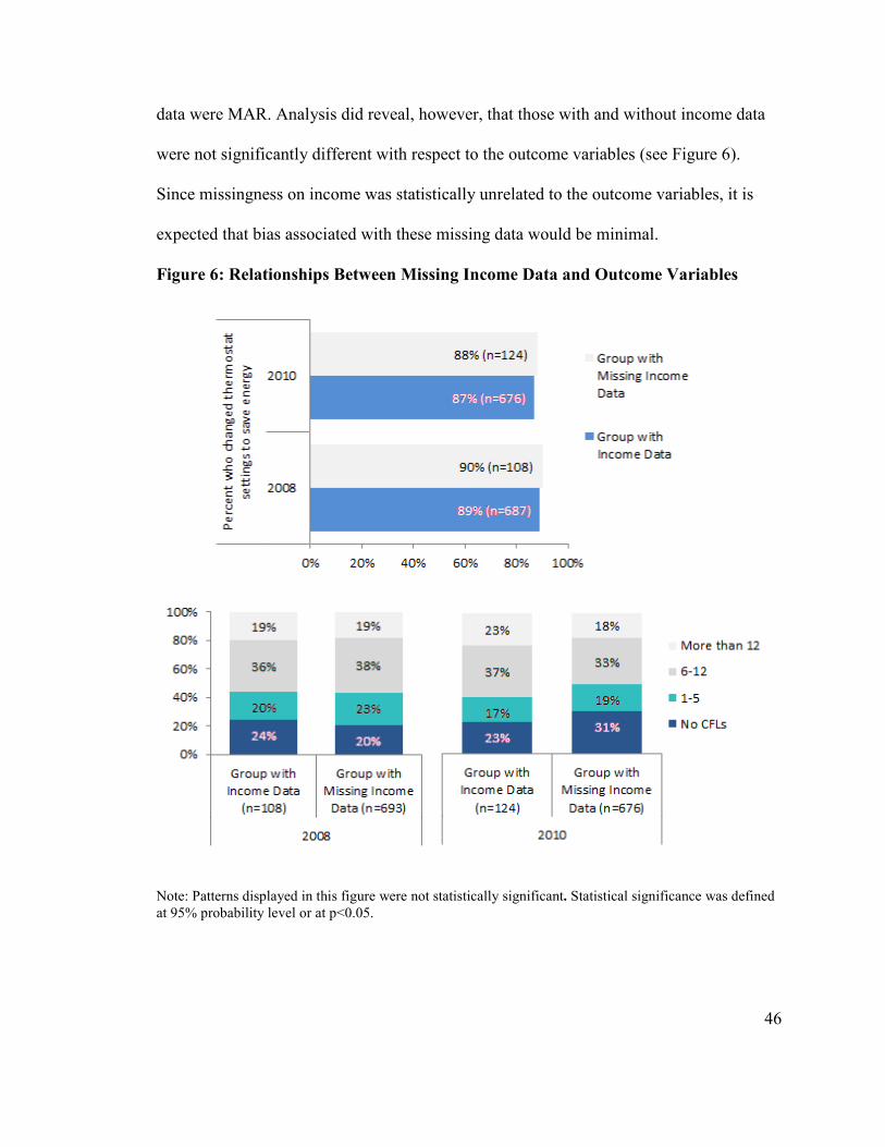
46

data were MAR. Analysis did reveal, however, that those with and without income data

were not significantly different with respect to the outcome variables (see Figure 6).

Since missingness on income was statistically unrelated to the outcome variables, it is

expected that bias associated with these missing data would be minimal.

Figure 6: Relationships Between Missing Income Data and Outcome Variables

Note: Patterns displayed in this figure were not statistically significant. Statistical significance was defined

at 95% probability level or at p<0.05.

47

5.2.2 Missing Data in the California Data Sample

To examine the relationships between attitudes and behaviors in the California

dataset, notable missing data issues had to be addressed prior to conducting relevant

analyses. Also, due to concerns about the survey length, researchers who implemented

the California survey asked one-quarter to one-half of respondents the attitudinal

questions. Those who were asked the attitudinal questions were randomly selected, which

indicates that missing data with respect to attitudinal variables were MCAR.

Since a large proportion of respondents in the 2010 sample were not asked the

attitudinal questions, this resulted in a small number of cases for executing relevant

analyses. Therefore, the missing attitudinal data in the 2010 sample were handled using

Multiple Imputation or ML estimation using SPSS or Mplus software (most analyses

were conducted using SPSS). Twenty imputed datasets and 500 iterations per each

imputation interval were specified when running the Multiple Imputation command in

SPSS. (For descriptions of these missing data methods, see Appendix B.)

5.2.3 Development of Attitudinal Measures

Researchers implementing the Energy Conservation, Efficiency, and Demand

Response national survey used a 5-point Likert scale to capture people's favorable and

unfavorable judgments regarding several environmental, financial, and behavioral

statements related to energy use. Specifically, the U.S. residents who took the survey

rated how much they agreed with various energy-related statements, using a scale from 1

48

to 5 where 1 meant “strongly disagree” and 5 meant “strongly agree.”11 Only nine

statements were presented using identical phrasing in all waves of the Energy

Conservation, Efficiency, and Demand Response survey. Table 8 lists these nine

statements.

Table 8

Nine Attitudinal Statements With Consistent Phrasing During All Waves of the Survey

(National Data)

Respondents Rated these Statements from 1=Strongly Disagree to 5=Strongly Agree

Environment statements

1. I’m very concerned about the environment.


3. Saving energy helps the environment.

Statements about the cost of energy



Statements about energy use in the society


7. There is an energy crisis in our country.



9. I’m too busy to be concerned with saving energy in my home.

Ratings of these nine items were examined to determine whether responses to

certain items measured a particular attitude. This was done because attitudes cannot

directly be observed (i.e., they are latent variables). To identify latent variables (i.e.,

11 Originally, the scale was from 1 to 5 where 1 meant “strongly agree” and 5 meant “strongly disagree.” This coding was reversed during the data cleaning step, so 1 became 5, 2 became 4, 3 became 3, 4 became

2 and 5 became 1.

49

highly correlated items that represent a larger attitudinal construct), Cronbach's alpha and

Confirmatory Factor Analysis (CFA) were employed to check for interdependencies

between the nine attitudinal items listed in Table 8. This was done by implementing the

following steps: (1) obtaining the correlation matrix between the attitudinal variables of

interest, (2) examining the coefficient of reliability (i.e., Cronbach's alpha), and (3) using

the Mplus CFA algorithm to test the model fit of a set of possible latent factors in the

data.12 The results of this procedure are discussed in Sections 6.1 and 7.1.

5.2.4 Analyses of the U.S. Survey Data

To evaluate the relationship between attitudes and those behaviors explored in

this study, logistic and ordinary least squares (OLS) regression analyses were conducted.

Logistic regression is used for dichotomous outcomes, and OLS regression is used for

continuous outcomes. In this study, thermostat-setting behavior was a dichotomous

variable or outcome (i.e., respondents reported whether [yes/no] they changed their

thermostat settings during the day, night, or seasonally to save energy), whereas CFL

installation behavior was a continuous variable (i.e., respondents reported the number of

CFL bulbs they had in their homes).

To test whether the attitudes explored in this study positively affect the adoption

of the selected behaviors (1st hypothesis) and whether any attitudinal effects on behavior

persist over time (2nd hypothesis), logistic and OLS regression analyses were conducted.

Logistic and OLS regression models also included, to the extent possible, important

12 Cronbach’s alpha determines if items have internal consistency – i.e., if they measure the same thing. The alpha values range from 0 to 1 and are higher when the correlations between items increase. Generally,

values of 0.7 or higher are acceptable indicators of reliability.

50

situational and external factors that can affect residential energy consumption behavior,

as noted in Section 3.4 and Table 9. It also is important to note that 2002-2010 datasets

were combined (pooled) and time variables representing the time-period during which the

data were collected were added to all logistic or OLS models.

Table 9

List of Variables Explored in this Study

Variable Type Description

Behavior 1. Thermostat-setting behavior (Yes/No as to whether they reported changing thermostat settings to save energy)

2. CFL installation (Reported number of CFLs in the home)

Attitudinal

Items

3. Ratings of nine statements about the environment, energy cost, and energy use (Scale: 1-5, where 1 meant “strongly disagree” and 5 meant “strongly agree”)

Household- specific Variables

4. Awareness of ENERGY STAR Label (Yes/No)

5. Income (Categories: 1=less than $20k to 8=more than $80k)

6. Age (Years)

7. Home ownership (Renters or owners)

8. Household size (Number of people living in the home)

9. Type of residence (1=Single-family, 0=Apt., Duplex, Mobile, Manufactured)

10. Energy savings (Yes=saw savings on their energy bills after performing an action to save energy; No= had not seen any savings on their energy bills)

External Factors

11. HDD in respondent’s state of residence in the last 12 months prior to the interview

12. Retail price of heating fuel (cents/1000 BTU)

13. Price per CFL bulb in respondent’s region of residence (Regions are Northeast, the Midwest, the South, and the West.)

14. Dollars per capita spent on energy efficiency programs in the state of residence

To test whether household budget moderates the attitude-behavior relationships

explored in this study (3rd hypothesis), the attitude-income interaction terms, together

with time variables and terms listed in Table 9, were added to the logistic and OLS

regression models. The objective of this specification was to explore attitude-budget

interactions and their association with no-cost conservation actions (thermostat-setting

51

behavior) and low-cost energy efficiency behavior (CFL installation). Income was used

as a proxy for budget.

To assess whether attitude-behavior relationships are different across socio-

demographic groups (4th hypothesis), a Classification and Regression Tree (CART)

analysis was conducted. CART is a statistical method that examines whether attitude-

behavior relationships vary across any demographic or other subgroups in the data.

Specifically, CART determines which predictor values (independent variables) result in

the best differentiation of the observations based on the outcome variable. This method is

appropriate for this analysis because it does not require an analyst to specify which

groups or variables to explore in the dataset. That is, this method identifies all notable

attitude-behavior relationships across demographic, regional, or any other likely

subgroups in the datasets. (For additional information about CART, see Appendix C.)

5.2.5 Analyses of the California Data

To further explore attitude-behavior relationships, the California data were

examined. The focus of this analysis was two-fold: (1) to assess if attitude-behavior

patterns in this dataset were similar to those observed in the national datasets, and (2) to

assess whether any attitude-behavior relationships were different across regions that were

politically more conservative or liberal. This regional analysis was reasonable because

political ideologies in an area may influence residents’ attitudes regarding energy use.

Similar regression analyses, discussed in the preceding section, were conducted when

analyzing the California data.

52

5.2.6 Modeling Limitations

When modeling attitude-behavior relationships, modeling misspecification is an

important issue to consider. Regression models can be mis-specified if important

variables are omitted or if the direction of the relationship between attitudes and

behavior, for example, is reversed. This section documents limitations of the modelling

work performed in this study to alert the reader that regression results in chapters 6 and 7

should be interpreted with caution.

Omitted Variable Bias

Omitted variable bias is a concern in this study. Due to lack of data, the regression

models, discussed in chapters 6 and 7, included only some of the important variables

and/or factors that could have explained the adoption of thermostat-setting or CFL

installation behavior (see Figure 7). Specifically, several factors were omitted from the

models: (1) attitudes on comfort, social norms, and perceived costs with respect to the

behaviors examined in this study, (2) knowledge of CFL incentives or subsidies in the

region of residence, (3) awareness that thermostat-setting behavior has notable energy

savings potential, (4) house age and/or structural attributes of a home, (5) ages of others

in the home, and (6) broader but relevant energy policy context around building codes

and/or products. In addition to these factors, there are likely other variables that influence

the adoption of behaviors investigated in this study, which also are missing from the

regression models (e.g., unobservable preferences such as dislike of CFL lights.).

53

Figure 7: Factors Influencing Energy Use Identified from the Literature Review

Bold text denotes omitted variables from the regression models in chapters 6 & 7, due to lack of data.

Some of the omitted variables referenced above could be correlated with variables

included in the regression models. For example, knowledge of CFL incentives or

knowing which no-cost behavior has a notable energy savings potential could be

correlated with dollars spent on energy efficiency programs in the region of residence, a

variable currently included in both thermostat-setting and CFL installation regression

models. Some portion of funding for energy efficiency programs often is spent on

Individual

1. Perceptions about: conservation, comfort, social norms, and perceived costs (Limited data; examination of only two conservation-related attitudes: concern for the environment and concern for energy use in the U.S. society)

2. Age

3. Pertinent knowledge (Limited data; have data only on awareness of ENERGY STAR label - a label that identifies which products are efficient in the marketplace)

Environment

Structure

1. Home size (Included house type variable -single-family, duplex, apartment, etc.- as a proxy for home size)

2. Home age

3. R-value of insulation

4. Equpiment type (appliances, HVAC, etc.)

External

1. Weather (Included HDD data)

2. Energy/product prices (Included heating fuel and CFL prices)

3. Energy efficiency (EE) programs (Included data on $ spent per capita on EE programs in the state of residence)

4. Building codes and appliance standards (No data, but included region since these factors vary by region)

Households

1. Ages (young, elderly)

2. Home owners

3. Someone handy at home (Not applicable to the behaviors tested in this study)

4. Income

5. Number of occupants

54

campaigns that attempt to raise public awareness and knowledge of energy-saving

behaviors and available incentives among the target population. These campaigns also

focus on emphasizing the environmental and financial benefits of saving energy, which in

turn, could affect the attitudes of those exposed to such campaigns. Thus, a lack of

pertinent knowledge variables, such as those referenced above, could be a source of bias.

That is, there is a possibility that some of the variables omitted due to lack of data are

correlated with those variables included in the regression models. When omitted variables

are correlated with independent variables in a regression model, the regression model

produces biased estimates.

Selection Bias in Regression Models

Selection bias can occur when the selection of respondents is not sufficiently

random to draw a general conclusion. The 2002 to 2010 national samples and the 2010

California sample were randomly generated. However, all samples underrepresented

younger adults, renters, and less-educated individuals, which is an indication that the

regression estimates, discussed in chapters 6 and 7, could be vulnerable to the selection

bias. Additionally, a notable proportion (58% in 2004, 42% in 2006, 24% in 2008, and

24% in 2010) of respondents in the national samples had not adopted CFLs. Similarly, a

notable proportion (27%) of respondents in the California sample reported having no

CFLs in their homes. When comparing those who had and had not adopted CFLs, several

striking patterns emerged. In the national data, those not adopting any CFLs were

significantly different in age (younger) than those adopting CFLs (see results of logistic

regression Model 9 in Chapter 6). In contrast, age was not a significant predictor in the

model examining the number of CFLs individuals had in their home (see OLS regression

55

Model 8 in Chapter 6). In the California data, the general environmental attitude, income,

house type, number of occupants, race/ethnicity besides “white” or “Hispanic,” and

average monthly energy bill were not significant predictors of those who had and had not

adopted CFLs (see logistic regression Model 2 in Chapter 7) and were significant

predictors in the model examining the number of CFLs individuals had in their home (see

OLS regression Model 1 in Chapter 7). These findings, especially those with respect to

age (since in all samples, younger adults were underrepresented), indicate that the

regression coefficients might be vulnerable to the sample selection bias. When there is a

selection bias in gathered data, the regression models such as OLS could yield biased

estimates of the effects of the independent variables on the dependent variable.

Reverse Causality

The models tested in this study assume that attitudes can explain behavior instead

of the opposite: that behavior can explain attitudes. This specification was intentional

because there is evidence in the literature that conservation or energy efficiency attitudes

cause changes in energy-related behaviors (Fishbein & Ajzen, 1975; Ajzen, 1991; Stern,

2007; Nolan et al., 2008).

However, there is a possibility of reverse causality or that attitudes and behaviors

occur simultaneously. Given this possibility, additional analysis was performed to

identify “instrumental variables.” Instrumental variables are those that would provide

some indication of a need to consider reverse causality. These variables would be

uncorrelated with the error term of the outcome variable and correlated with the

independent variables in the regression model. In both the national and California data,

variables uncorrelated with the CFL installation behavior had very low correlations (less

56

than or approximately 0.1) with other independent variables in the regression models,

except for the correlation between the pro-environmental attitude and the attitude about

energy use in the U.S. society (r=0.5). A similar pattern was observed with the data for

the thermostat-setting model – that is, several variables uncorrelated with the thermostat-

setting behavior had very low correlations (less than or approximately 0.1) with nearly all

independent variables in the regression models. In a few instances when correlations

were above 0.1, the correlations ranged from being weak to moderate (between 0.3 and

0.5). These findings indicate that one cannot with confidence determine that there are any

good candidates for instrumental variables in the available data.

Still, it is important to acknowledge that the current regression models have not

been modeled in a manner that would take into account, to an extent, an issue of reverse

causation. Not doing this could be a source of bias with respect to the modeling work

performed in this study. One can imagine a scenario where an individual engages in an

energy-saving behavior, such as buying a CFL bulb, and then developing an attitude that

a CFL light looks terrible (after they installed and tested it), which will make them not

want to purchase another CFL. There is some evidence that past behavioral experiences

correlate moderately with attitudes (Regan & Fazio, 1977; Fazio & Zanna, 1981), and

that past behaviors can be significant predictors of attitudes associated with an

environmentally friendly behavior such as recycling (Knussen & Yule, 2009). This

literature indicates that there is a possibility that behaviors can explain attitudes.

Given this possibility, the unidirectional behavioral models discussed in this study

could be more complex than what has been shown in this thesis.

57

Heteroscedasticity

The Breusch-Pagan test of the regression models was conducted to check for

heteroscedasticity.13 The test showed heteroscedasticity was an issue. To address this

issue, the robust standard errors were estimated for each OLS regression model.

However, this was not possible for the logistic regression models because the SPSS

software did not have an option to estimate robust standard errors for these models.

13 Heteroscedasticity occurs when there are systematic patterns in the variance of the error terms across

observations.

58

6. FINDINGS FROM THE NATIONAL DATASETS

This section documents descriptive statistics and the results of the Cronbach's

alpha, CFA, and regression analyses.

6.1 Assessment of Attitudinal Items

6.1.1 Descriptive Statistics

Table 10 displays the average ratings of the nine statements that may represent a

larger attitudinal construct. Frequencies of these responses are displayed in Appendix A.

59

Table 10

Nine Statements (Means)

Respondents Rated the Following Statements

From 1=Strongly Disagree to 5=Strongly

Agree

2002

(n=900)

2004

(n=801)

2006

(n=800)

2008

(n=801)

2010

(n=800)

Env. 1. I’m very concerned about the environment.

4.2 4.2 4.2 4.3 4.2


3.9 4.0 4.0 4.0 4.0


4.2 4.3 4.3 4.2 4.2

Cost of

energy


4.1 4.1 4.1 4.2 4.1


3.0 2.9 3.0 3.1 3.0

Energy

use in

the

society


3.6 3.9 3.9 3.8 3.8


3.6 3.9 3.8 4.1 3.8

Saving

energy

at

home


2.9 3.2 3.2 3.2 3.3


2.0 2.0 1.9 1.9 1.9

Note: Means reported in this table are estimated using Full Maximum Likelihood (FIML) missing data estimation. There were no notable differences in estimations of the means when using listwise deletion

compared to FIML missing data estimation.

6.1.2 Cronbach's Alpha

Computation of Cronbach's alpha was the first step in identifying latent variables

or highly correlated items that represent a larger attitudinal construct. Specifically,

Cronbach's alpha was used to check for internal consistency or reliability between the

attitudinal items in all the datasets. The three pro-environmental items, listed in Table 11,

had the highest Cronbach's alpha values (0.65 in 2002, 0.70 in 2004 and 2006, 0.69 in

2008, and 0.72 in 2010). The two items about energy use in the U.S. society had the

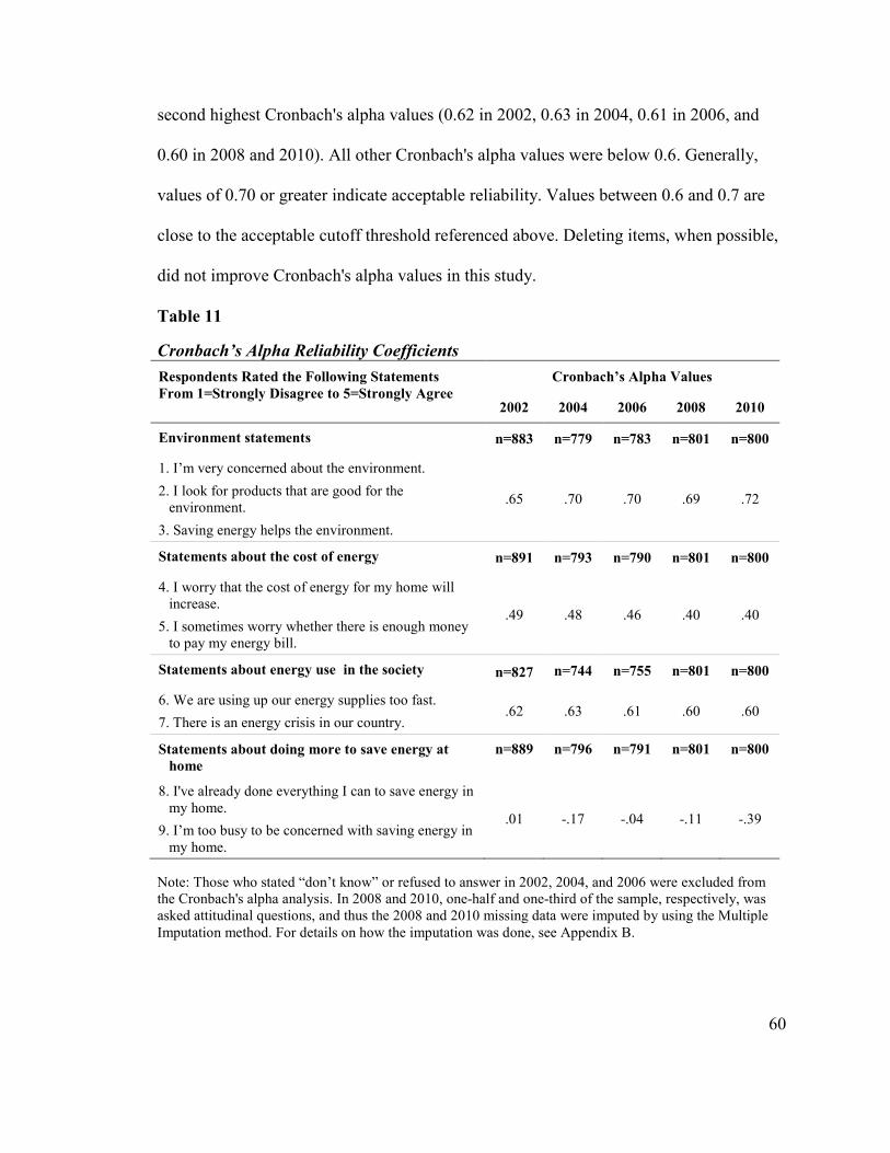
60

second highest Cronbach's alpha values (0.62 in 2002, 0.63 in 2004, 0.61 in 2006, and

0.60 in 2008 and 2010). All other Cronbach's alpha values were below 0.6. Generally,

values of 0.70 or greater indicate acceptable reliability. Values between 0.6 and 0.7 are

close to the acceptable cutoff threshold referenced above. Deleting items, when possible,

did not improve Cronbach's alpha values in this study.

Table 11

Cronbach’s Alpha Reliability Coefficients

Respondents Rated the Following Statements

From 1=Strongly Disagree to 5=Strongly Agree Cronbach’s Alpha Values

2002 2004 2006 2008 2010

Environment statements n=883 n=779 n=783 n=801 n=800

1. I’m very concerned about the environment.



.65 .70 .70 .69 .72

Statements about the cost of energy n=891 n=793 n=790 n=801 n=800



.49 .48 .46 .40 .40

Statements about energy use in the society n=827 n=744 n=755 n=801 n=800


7. There is an energy crisis in our country. .62 .63 .61 .60 .60

Statements about doing more to save energy at

home n=889 n=796 n=791 n=801 n=800



.01 -.17 -.04 -.11 -.39

Note: Those who stated “don’t know” or refused to answer in 2002, 2004, and 2006 were excluded from the Cronbach's alpha analysis. In 2008 and 2010, one-half and one-third of the sample, respectively, was asked attitudinal questions, and thus the 2008 and 2010 missing data were imputed by using the Multiple

Imputation method. For details on how the imputation was done, see Appendix B.

61

6.1.3 CFA Results

CFA was the second step in identifying latent variables or highly correlated items

that represent a larger attitudinal construct. Specifically, CFA was used to test whether

data fit a hypothesized two-factor structure inferred from the preceding analysis. That is,

whether environmental items (those with the highest Cronbach's alpha values) measured

the pro-environmental attitude, and whether items about energy use in the society (those

with the Cronbach's alpha values close to the acceptable cutoff threshold) measured the

societal energy-use attitude. Figure 8 displays the hypothesized two-factor CFA model.

62

Figure 8: Hypothesized Two-factor Structure (2002-2010 National Data)

CFA results show that 2002 and 2006 two-factor models had significant chi-

square values, 2004 and 2010 models had marginally significant chi-square values, and

the 2008 model had a non-significant chi-square value (see Table 12). Although a

significant chi-square value indicates poor fit to the data, this value is affected by the

sample size (i.e., it is almost always statistically significant when the sample size is

large). Because of this limitation, the alternative fit indices were examined to determine

whether the two-factor models fit the data adequately. According to standards suggested

by Hu and Bentler (1999) and MacCallum, Browne, and Sugawara (1996), the alternative

fit indices suggested an acceptable fitting model. As shown in Table 12, CFI was between

I’m very

concerned

about the

environment

I look for

products that

are good for the

environment

Saving energy

helps the

environment

Pro-

environmental

attitude

We are using up

our energy

supplies too

fast

There is an

energy crisis in

our country

Societal energy use attitude

e1

e2

e3

e4

e5

Factor

Correration

Factor

loading

Errors

63

.97 and .99, RMSEA was between .03 and .06, and SRMR was between .01 and .06 from

2002 to 2010. According to MacCallum, Browne, and Sugawara (1996), for CFI, a value

close to one indicates a good-fitting model; for RMSEA and SRMR a value below 0.08

indicates a good-fitting model. A comparison of the one-factor model and the two-factor

model indicated that the two-factor model fit better than the one-factor model. The two-

factor model had higher CFI and lower RMSEA and SRMR values across all samples

than the one-factor model.

Table 12

Goodness-of-Fit Indicators of Two-Factor CFA Model

Model χ2(df) RMSEA SRMR CFI

2002 (n=900) 17.5(4)** 0.06 0.02 0.98

2004 (n=801) 8.2(4)ᵻ 0.04 0.01 0.99

2006 (n=800) 17.0(4)** 0.06 0.02 0.99

2008 (n=801) 6.1(4) 0.03 0.03 0.99

2010 (n=800) 9.5(4)ᵻ 0.05 0.06 0.97

**Significant at p<0.05; ᵻ Marginally Significant at p<0.1

Note: Results reported in this table are estimated using Full Maximum Likelihood (FIML) missing data estimation. Missing data were an issue in 2008 and 2010 samples; one-half and one-third of the respondents in 2008 and 2010, respectively, were asked the attitudinal questions.

The results also suggest that the three environmental items had significant

standardized loadings on the first factor (see Table 13). Similarly, the two items about

societal energy use had significant standardized loadings on the second factor (see Table

13). Estimated correlations among factors were significant (p<.05) in all models and were

0.74 in 2002, 0.78 in 2004, 0.79 in 2006, 0.73 in 2008, and 0.67 in 2010.

64

Table 13

Unstandardized (Standardized) Loadings of Two-Factor CFA Model 2002

(n=900)

2004

(n=801)

2006

(n=800)

2008

(n=801)

2010

(n=800)

Pro-environmental Attitude (Factor 1)

I’m very concerned about the environment.

1.12 (.68)**

1.28 (.72)**

1.24 (.69)**

0.997 (.68)**

1.34 (.86)**

I look for products that are good for the environment.

0.99 (.57)**

1.20 (.64)**

0.99 (.56)**

0.87 (.56)**

1.15 (.73)**

Saving energy helps the environment.

1.00

(.61)** 1.00

(.64)** 1.00

(.69)** 1.00

(.73)** 1.00

(.61)**

Societal Energy Use Attitude (Factor 2)

We are using up our energy supplies too fast.

1.10 (.72)**

1.20 (.75)**

1.14 (.72)**

1.41 (.74)**

1.03 (.71)**

There is an energy crisis in our country.

1.00

(.62)**

1.00

(.63)** 1.00

(.61)** 1.00

(.59)** 1.00

(.73)**

** Significant at p<0.05; ᵻ Marginally Significant at p<0.1

Note: Results reported in this table are estimated using Full Maximum Likelihood (FIML) missing data estimation. Missing data were an issue in 2008 and 2010 samples; one-half and one-third of the respondents

in 2008 and 2010, respectively, were asked the attitudinal questions.

6.1.4 Attitudinal Measures

As noted in the preceding sections, Cronbach’s alpha values were at or near the

acceptable cutoff threshold for the environmental items and items about energy use in the

U.S. society. The CFA results indicated that the standardized loadings for these items

were high and, overall, the CFA results suggested that the hypothesized two-factor model

represented the data well. Based on these findings, the respondents’ agreement ratings

with the three environmental statements and two statements about energy use in the U.S.

society were averaged for each case in the dataset to produce two attitudinal scores: (1) a

score reflecting the respondent’s level of concern for the environment, and (2) a score

reflecting the respondent’s level of concern about the energy situation in the U.S. society.

65

Lower scores indicate less concern for the environment or energy use in the U.S. society,

whereas higher scores indicate greater concern for the environment or energy use in the

U.S. society.

Table 14

Mean Scores of the Two Attitudinal Measures 2002 2004 2006 2008 2010

n=883 n=779 n=783 n=801 n=800

Pro-environmental score (average ratings of three environmental statements; lower/higher scores mean lower/higher concerns for the environment)

4.1 4.2 4.2 4.2 4.1

n=891 n=793 n=790 n=801 n=800

Score reflecting how respondents think about energy use in the U.S. society (average ratings of two statements about energy use in the U.S. society; lower/higher scores mean lower/higher concerns about energy use in the U.S. society)

3.6 3.9 3.9 4.0 3.8

Note: Those who stated “don’t know” or refused to answer in 2002, 2004, and 2006 were excluded from this analysis. In 2008 and 2010, missing data were imputed by using the Multiple Imputation method. One-half and one-third of the 2008 and 2010 sample, respectively, was asked attitudinal questions. For details

on how the imputation was done, see Appendix B.

6.1.5 Items Excluded in the Subsequent Analyses

Among nine items shown in Table 10, only five were combined to create two

attitudinal measures, as explained in the preceding sections. All but two of the rest of the

items were excluded from the subsequent analyses since it was unclear what larger

attitudinal or latent construct they measure. The two items not combined to create an

attitudinal measure but included in the subsequent analyses were: "I worry that the cost of

energy for my home will increase" and "I sometimes worry whether there is enough

money to pay my energy bill.” These two items, together with income, contain

66

information about a respondent's economic situation, which is an important consideration

when modeling energy-use behavior. For this reason, these two items were included in

the subsequent regression analyses as separate items and were not considered to be

attitudinal measures.

6.2 Assessment of Behavioral Variables

6.2.1 Thermostat-setting Behavior

A question about whether respondents had one or more thermostats in their homes

was included in the 2002, 2004, and 2006 survey questionnaires. In exploring responses

to this question, it was observed that not all respondents had access to a thermostat in

their homes. Only about three-quarters of respondents who agreed to take the survey in

2002, 2004, and 2006 reported having one or more thermostats that control heating

and/or cooling in their homes (see Table 15). This is important to note because those

households without access to a thermostat were physically restricted from having the

option to change thermostat settings to save energy at home.

Table 15

Access to a Thermostat

Percent Reporting… 2002 (n=898) 2004 (n=800) 2006 (n=799)

One or more thermostats at home 78% 72% 78%

No thermostats at home 22% 28% 22%

Note: Those who refused to answer were excluded from this analysis.

Further analysis revealed that lower-income households compared to higher-

income households and renters compared to owners were less likely to have access to a

thermostat, across the 2002-2006 samples (see Figure 9 and Figure 10). Similarly, those

67

living in a duplex, apartment, mobile home, or manufactured home were less likely to

report having access to a thermostat than those living in a single-family home in 2002

and 2006 (see Figure 11).

Figure 9: Percentage of Cases Without Thermostat Access by Household Income

Note: Pearson chi-square was significant at p<0.05 in all samples.

Figure 10: Percentage of Cases Without Thermostat Access by Home Ownership

Note: Pearson chi-square was significant at p<0.01 in all samples.

28%

16% 14%

32%23% 20%

28% 24%

11%

Up to

$50,000

(n=460)

$50,000

up to

$80,000

(n=189)

Over

$80,000

(n=123)

Up to

$50,000

(n=348)

$50,000

up to

$80,000

(n=158)

Over

$80,000

(n=138)

Up to

$50,000

(n=347)

$50,000

up to

$80,000

(n=178)

Over

$80,000

(n=174)

2002 2004 2006

35%

19%

39%

26%33%

20%

Renters

(n=210)

Owners

(n=677)

Renters

(n=154)

Owners

(636)

Renters

(n=121)

Owners

(n=669)

2002 2004 2006

68

Figure 11: Percentage of Cases Without Thermostat Access by House Type

Note: Pearson chi-square was significant at p<0.05 in 2002 and 2006 samples.

Households without access to a thermostat were excluded from the subsequent

logistic regression analyses because the goal was to examine the attitudinal effect on

thermostat-setting behavior among those who had the ability to change thermostat

settings in their homes. When those without access to a thermostat were excluded from

the analyses, it was found that the vast majority of households with access to a thermostat

reported changing a thermostat setting to save energy at home (see Figure 12).

28%

21%

33%28%

32%

19%

Other Home

Types

(n=234)

Single

Family

(n=659)

Other Home

Types

(n=162)

Single

Family

(n=629)

Other Home

Types

(n=141)

Single

Family

(n=653)

2002 2004 2006

69

Figure 12: Percentage of Cases Reporting Thermostat-setting Behavior Among

Those with Access to a Thermostat

It is important to note that there are few no-cost conservation behaviors that

individuals can implement. In addition to thermostat-setting behavior, individuals can

turn off lights when not in use; unplug or turn off equipment (appliances, computers, etc.)

when not in use; close rooms off when not in use; open windows and doors to cool; close

drapes to reduce interior heating; and minimize the amount of hot water used by taking

shorter showers, lowering temperature settings on the water heater, or using full loads

when washing dishes or laundry. Among these no-cost actions, thermostat-setting

behavior has the greatest energy savings potential, mainly because the U.S. households,

on average, spend about 42% and 6% of the total energy used at home on space heating

and cooling, respectively (EIA Residential Energy Consumption Survey, 2009). Since

U.S. households spend so much energy on heating and cooling, it is important to study

thermostat-setting behavior.

Although the vast majority of respondents reported changing a thermostat setting

to save energy, it is not known how often or to what extent these households engaged in

this behavior. Therefore, it is unclear whether this behavior is routine for many

84%

90% 89%

Cases with access to a

thermostat who did the

behavior (n=697)



behavior (n=568)



behavior (n=623)

2002 2004 2006

70

respondents or whether respondents change their thermostat settings by a significant

margin (e.g., 10°F or more). Because the 2002-2006 surveys did not capture this level of

detail, this study can examine only differences between those who had not performed this

behavior and those who had performed it to some extent.

The lack of detail regarding how often and how much respondents adjusted their

thermostat settings to save energy is a limitation of this study. Prior research had shown

that those who adjusted their thermostats often had significantly lower nighttime

thermostat settings (Peters, 1989), indicating that some individuals routinely alter their

thermostat settings to a significant degree and some do not. In this study, it was not

possible to differentiate between those who did or did not routinely alter their thermostat

settings to a significant degree due to lack of examinable data. Nevertheless, it is valuable

to examine differences between those who had never performed this behavior and those

who had performed it to some extent (as reflected in the gathered data) because

researching those who had performed this behavior could yield information regarding

why people engage in no-cost and simple-to-perform behaviors, such as thermostat-

setting behavior, that can be leveraged when developing interventions to encourage such

behaviors.

6.2.2 CFL Installation Behavior

Unlike thermostat-setting behavior, all survey respondents had the ability to

install CFL bulbs in their homes. The respondents reported the number of CFL bulbs they

had in their homes, which is an indicator of whether they had installed just one or more

71

than one CFL bulb in their homes. The percentage of those who installed one or more

than one CFL bulb increased substantially from 2004 to 2010 (Table 16).14

Table 16

Number of CFL Bulbs in the Home

Number of CFLs 2004 (n=798) 2006 (n=798) 2008 (n=801) 2010 (n=800)

0 CFLs 58% 42% 24% 24%

1-5 24% 29% 21% 17%

More than 5 18% 29% 55% 59%

Mean 2.8 4.6 8.5 9.1


6.3 Attitudes and Thermostat-setting Behavior

This section summarizes notable findings from descriptive and logistic regression

analyses that explored the associations among the two attitudes referenced above,

thermostat-setting behavior, and several additional situational and external variables.

6.3.1 Bivariate Descriptive Statistics

The 2002 to 2006 datasets were combined into one dataset.15 Initial analysis of

this pooled data revealed that the pro-environmental attitude and the attitude about

societal energy use had a significant and moderate correlation (r =.51). All other

significant correlations noted in Table 17 were weak.

14 In 2002, respondents were not asked how many CFL bulbs they had in their homes. For this reason, the

2002 data were excluded from this analysis.

15 The 2008 and 2010 data lacked a variable that identified those with and without access to a thermostat in

the home. For this reason, these data were not used in this and subsequent logistic regression analyses.

72

Table 17

Correlations Among Attitudes, Behavior, and Time (Pooled 2002-2006 Data)

Pro-environmental

Attitude

Attitude About Societal

Energy Use

Thermostat-setting Behavior

– changed thermostat settings

to save energy (1=yes, 0=no)

.09** .04

Time 1: 2002 (2002=1, 2004=0, 2006=0)

-.04 -.14**

Time 2: 2004 (2002=0, 2004=1, 2006=0)

.03 .07**


Energy Use .51** --


Note: Only those with access to a thermostat were included in this analysis. Missing data were excluded

from this analysis.

6.3.2 Modeling Attitudinal Effect on Thermostat-setting Behavior

Logistic regression analyses were conducted to test whether attitudes explored in

this study are positively associated with thermostat-setting behavior (1st hypothesis), and

whether any attitudinal effects on this behavior persist over time (2nd hypothesis). To test

these hypotheses, associations among thermostat-setting behavior and attitudes toward

the environment and societal energy use were explored together with several important

demographic and external factors that may have an effect on whether respondents with

access to a thermostat engage in thermostat-setting behavior.

The first logistic regression model examined the attitude-behavior relationships,

while controlling for time.16 Table 18 displays the results (odds ratios). Odds ratios

16 The 2008 and 2010 data lacked a variable that identified those with and without access to a thermostat in

the home. For this reason, these data were not used in this analysis.

73

measure the likelihood that those who had engaged in thermostat-setting behavior were

different from those who had not done that action. Values above and below “1” mean that

those who had engaged in thermostat-setting behavior were more likely or less likely,

respectively, to have other distinct characteristics than those who had not done that

action. Results show that for each unit increase in the pro-environmental attitudinal score,

the odds of changing thermostat settings to save energy significantly increased by 1.7

among those who had access to a thermostat. Results also show that those in 2002 were

significantly less likely than those in 2006 to engage in thermostat-setting behavior. This

model, shown in Table 18, explained a very small amount of variance; pseudo R² value

was 0.04. The overall model fit was significant (χ=32.8, p<0.05).

74

Table 18

Logistic Regression Model 1 Results (Pooled 2002-2006 Data)

Variables Description Odds Ratios (n=1731)

Attitudes Env. Attitude - average pro-environmental score (lower/higher scores mean lower/higher concerns for the environment)

1.7**

Soc. Energy Attitude - average score denoting concern about energy use in the U.S. society (lower/higher scores mean lower/higher concerns about energy use in the U.S. society)

.91

Time 2002 (2002=1, 2004=0, 2006=0) .56**

2004 (2002=0, 2004=1, 2006=0) 1.1

Pseudo R² (Nagelkerke R²) .04

Model Fit Statistics (Chi-square value and Significance) 32.8, p<.01


Note 1: The dependent variable is thermostat-setting behavior (1=Yes, 0=No). Only those with access to a

thermostat were included in this analysis. Missing data were excluded from this analysis.

Note 2: This model also was tested by including factor scores instead of composite scores (i.e., average rating scores of the items loading into a factor). Both approaches (using factor or composite scores) yielded similar results. This model also was run as a probit model; the findings (pseudo R² and significance of the coefficients) from a probit model were the same as in this logit model.

To assess whether attitude-behavior relationships explored in this study are

different across time (i.e., from 2002 to 2006), the logistic regression models 2-5, shown

in Table 19, included all the variables from the preceding model and several interaction

terms between the two attitudes referenced above and time variables. The interaction

terms were included to test whether attitude-behavior relationships depended on time.

The interaction terms were constructed by multiplying attitudinal variables and time

variables. In all the models, the interaction terms were not significant (Table 19).

75

Table 19

Logistic Regression Model 2-5 Results (Pooled 2002-2006 Data)


Odds Ratios (n=1731)

Model

2

Model

3

Model

4

Model

5


1.7** 1.6** 1.6** 1.6**


.91 .91 .96 .86

Time 2002 (2002=1, 2004=0, 2006=0) .76 .56** .80 .55**

2004 (2002=0, 2004=1, 2006=0) 1.1 .84 1.1 .54

Interactions Env. Attitude * 2002 .93 -- -- --

Env. Attitude * 2004 -- 1.1 -- --

Soc. Energy Attitude * 2002 -- -- .91 --

Soc. Energy Attitude * 2004 -- -- -- 1.2

Pseudo R² (Nagelkerke R²) .04 .04 .04 .04

Model Fit Statistics (Chi-square value and

Significance)

32.9,

p<.01

32.9,

p<.01

33.2,

p<.01

33.7,

p<.01


Note 1: The dependent variable is thermostat-setting behavior (1=Yes, 0=No). Only those with access to a thermostat were included in this analysis. Missing data were excluded from this analysis.

Note 2: These models also were tested by including factor scores instead of composite scores (i.e., average rating scores of the items loading into a factor) and by running the models as probit models. All approaches

yielded similar results.

To assess how the thermostat-setting behavior would vary with a percent change

in the attitude score, the elasticity of the environmental attitude was calculated using the

environmental attitude regression parameter from Model 1.17 Elasticity is an indicator of

how responsive one variable is to a change in another. The elasticity was 0.24. This

means that one percentage point increase on the attitude scale would increase the

17 The elasticity was computed using STATA statistical software.

76

probability of adopting the thermostat-setting behavior by about quarter of a percentage

point (a small but not negligible effect). Alternatively, ten percentage point increase on

the attitude scale would increase the probability of adopting thermostat-setting behavior

by about 2.5 percentage points.

Because it is known that external conditions and demographic characteristics also

affect residential energy use, as shown in Figure 13, the next logistic regression model,

Model 6, explores attitude-behavior relationships while controlling for time and several

important external and demographic characteristics. Figure 13 shows all variables

included in the subsequent regression model.

77

Figure 13: Demographic and External Factors That Can Influence Energy-use

Behavior Identified from the Literature Review

Variables in red are present in the data and are included in the subsequent regression models.

In Model 6, four variables were significant: the environmental attitude, household

income, age, and number of occupants (see Table 20). One variable was marginally

significant: dollars spent per capita on energy efficiency programs in the state of

residence (see Table 20). These findings show that the environmental attitude (an attitude

that was significant in the prior models) remained significant when controlling for

external and demographic characteristics.

The overall logistic regression models explained a small amount of variance; the

pseudo R² value was 0.08. The overall model fit was significant (χ=55.8, p<0.05).

Individual

1. Perceptions about: conservation, comfort, social norms, and perceived costs (Limited data; examining only two conservation-related attitudes: concern for the environment and concern for energy use in the U.S. society)

2. Age

3. Pertinent Knowledge

Environment

Structure

1. Home size (Limited data; included house type variable -single-family, duplex, apartment, etc.-as a proxy for home size)

2. Home age



External


2. Energy/product prices (Included heating fuel price data)

3. Energy efficiency (EE) programs(Included data on $ spent per capita on EE programs in the state of residence)


Households


2. Home owners

3. Someone handy at home

4. Income


78

Table 20

Logistic Regression Model 6 Results (Pooled 2002-2006 Data)

Variables Description Odds Ratios

(n=1364)

Attitudes Env. Attitude - average pro-environmental score (lower/higher scores mean lower/higher concern)

1.5**

Soc. Energy Attitude - average score denoting concern about energy use in the U.S. society (lower/higher scores mean lower/higher concern)

.91

Economic

Considerat-

ions

Household Income (Categories: 1=less than $20k to 8=more than $80k) 1.1**

I worry that the cost of energy for my home will increase (5-pt scale from 1=strongly disagree to 5=strongly agree)

1.1

I sometimes worry whether there is enough money to pay my energy bill (same 5-pt scale)

1.0

House and

Household

Attributes

Home Ownership (1=Own, 0=Rent) 1.2

House Type (1=Single-fFamily Home, 0=Other) 1.1

Number of people living in the home 1.3**

Age of Respondent (Years) 1.02**

Region Reside in the Midwest (Northeast=0, Midwest=1, South=0, West=0) .70

Reside in the South (Northeast=0, Midwest=0, South=1, West=0) .67

Reside in the West (Northeast=0, Midwest=0, South=0, West=1) .70

Residential

Energy Prices

Avg. Retail Price of Heating Fuel (cents/1000 BTU) in the state of residence 1.0

Weather Number of Heating Degree Days in the state of residence 1.0

Energy

Efficiency

Funding

$ per capita spent on energy efficiency programs in the state of residence

1.04ᵻ

Time 2002 (2002=1, 2004=0, 2006=0) .76

2004 (2002=0, 2004=1, 2006=0) 1.3




Note 1: The dependent variable is thermostat-setting behavior (1=Yes, 0=No). Only those with access to a

thermostat were included in this analysis. Missing data were excluded from this analysis.

Note 2: Respondents reported the type of fuel they used to heat their homes and their zip codes. This information was used to link the average state-level retail prices of electricity, natural gas, propane, and heating oil with each case in the dataset. Prices for these fuels were in $/kWh, $/Therm, and $/gallon, and

were converted to cents/1000 British Thermal Units (BTUs). BTU is a traditional unit of energy.

Note 3: This model also was tested by including factor scores instead of composite scores and by running

this model as a probit model. All approaches yielded similar results.

79

6.3.3 Exploring Attitude-Budget Interactions

This section discusses notable results from the logistic regression analyses, which

were used to explore the relationships between attitude-budget interactions and behavior.

It is hypothesized (3rd hypothesis) that budget moderates attitude-behavior relationships.

To assess this hypothesis, the following steps were executed: (1) multiplied household

income and environmental attitude, (2) multiplied household income and societal energy-

use attitude, and (3) added these two interaction terms to the regression models (models 7

and 8), while controlling for all those variables from the prior model (Model 6).

In Model 7, three variables were significant: the environmental attitude, age, and

number of occupants (see Table 21). In Model 8, four variables were significant: the

environmental attitude, income, age, and number of occupants (see Table 21). In both

models, one variable was marginally significant: dollars spent per capita on energy

efficiency programs in the state of residence (see Table 21). The interaction terms

(included to test whether attitude-behavior relationships depended on household income)

were not significant in either Model 7 or Model 8 (see Table 21).

The overall logistic regression models (models 7 and 8) explained a small amount

of variance; pseudo R² value was 0.08 in both models. The overall model fit was

significant for both models (χ model 7 =57.3 and χ model 8 =57.4, p<0.05).

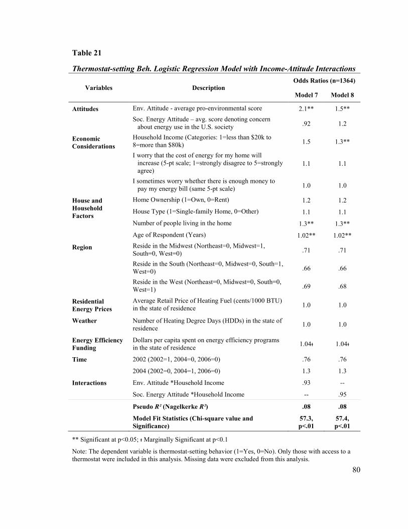
80

Table 21

Thermostat-setting Beh. Logistic Regression Model with Income-Attitude Interactions

Variables Description Odds Ratios (n=1364)

Model 7 Model 8

Attitudes Env. Attitude - average pro-environmental score 2.1** 1.5**

Soc. Energy Attitude – avg. score denoting concern about energy use in the U.S. society

.92 1.2

Economic

Considerations

Household Income (Categories: 1=less than $20k to 8=more than $80k)

1.5 1.3**

I worry that the cost of energy for my home will increase (5-pt scale; 1=strongly disagree to 5=strongly agree)

1.1 1.1


1.0 1.0

House and

Household

Factors

Home Ownership (1=Own, 0=Rent) 1.2 1.2

House Type (1=Single-family Home, 0=Other) 1.1 1.1

Number of people living in the home 1.3** 1.3**

Age of Respondent (Years) 1.02** 1.02**

Region Reside in the Midwest (Northeast=0, Midwest=1, South=0, West=0)

.71 .71

Reside in the South (Northeast=0, Midwest=0, South=1, West=0)

.66 .66

Reside in the West (Northeast=0, Midwest=0, South=0, West=1)

.69 .68

Residential

Energy Prices

Average Retail Price of Heating Fuel (cents/1000 BTU) in the state of residence 1.0 1.0

Weather Number of Heating Degree Days (HDDs) in the state of residence

1.0 1.0

Energy Efficiency

Funding

Dollars per capita spent on energy efficiency programs in the state of residence

1.04ᵻ 1.04ᵻ

Time 2002 (2002=1, 2004=0, 2006=0) .76 .76

2004 (2002=0, 2004=1, 2006=0) 1.3 1.3

Interactions Env. Attitude *Household Income .93 --

Soc. Energy Attitude *Household Income -- .95

Pseudo R² (Nagelkerke R²) .08 .08

Model Fit Statistics (Chi-square value and

Significance)

57.3,

p<.01

57.4,

p<.01


Note: The dependent variable is thermostat-setting behavior (1=Yes, 0=No). Only those with access to a thermostat were included in this analysis. Missing data were excluded from this analysis.

81

6.3.4 Exploring Attitude-Socio-Demographic Interactions

Stern (2007) observed that the effect of personal variables, such as attitudes, on a

behavior is dependent on contextual or situational variables such as availability of new

technology, the financial cost of adopting a behavior, and other such factors (p. 374,

conclusion #4). Income is one type of situational variable. Demographic and external

factors, such as household size or price of energy, are other types of situational variables.

To test whether other situational variables, besides income, moderate attitude-behavior

relationships, several interaction terms were created by multiplying the two attitudinal

variables by those situational and external variables present in the data: (1) home

ownership, (2) respondent’s age, (3) household size (# of people living in the home), (4)

house type (if single-family detached or other type of home), (5) average retail price of

heating fuel in the state of residence, (6) number of HDDs in the state of residence, and

(7) dollars per capita spent on energy efficiency programs in the state of residence.

No significant interaction terms were observed in any of the logistic regression

models that included these interaction terms (see Table 22). Models 9-24 explained a

small amount of variance; pseudo R² values were 0.08 in all models. The overall model

fit was significant for all models (see Table 22).

82

Table 22

Thermostat-setting Logistic Regression Model with Socio-Demographic-Attitude

Interactions


Note: The dependent variable is thermostat-setting behavior (1=Yes, 0=No). Only those with access to a thermostat were included in this analysis. Missing data were excluded from this analysis.

9 10 11 12 13 15 16 17 18 19 21 22 23 24

Env. Attitude * Home Ownership 0.6 -- -- -- -- -- -- -- -- -- -- -- -- --

Soc. Energy Attitude * Home

Ownership-- 0.8 -- -- -- -- -- -- -- -- -- -- -- --

Env. Attitude * House Type -- -- 0.8 -- -- -- -- -- -- -- -- -- -- --

Soc. Energy Attitude * House Type -- -- -- 0.9 -- -- -- -- -- -- -- -- -- --

Env. Attitude * # of people living in

the home-- -- -- -- 1.1 -- -- -- -- -- -- -- -- --

Soc. Energy Attitude * # of people

living in the home-- -- -- -- -- 1 -- -- -- -- -- -- -- --

Env. Attitude * Age -- -- -- -- -- -- 1 -- -- -- -- -- -- --

Soc. Energy Attitude * Age -- -- -- -- -- -- -- 1 -- -- -- -- -- --

Env. Attitude * Avg. Retail Price of

Heating Fuel-- -- -- -- -- -- -- -- 0.9 -- -- -- -- --

Soc. Energy Attitude * Avg. Retail

Price of Heating Fuel-- -- -- -- -- -- -- -- -- 0.9 -- -- -- --

Env. Attitude * HDD -- -- -- -- -- -- -- -- -- -- 1 -- -- --

Soc. Energy Attitude * HDD -- -- -- -- -- -- -- -- -- -- -- 1 -- --

Env. Attitude * $/capita spent on

energy efficiency programs in the state

of residence

-- -- -- -- -- -- -- -- -- -- -- -- 1 --

Soc. Energy Attitude * $/capita spent

on energy efficiency programs in the

state of residence

-- -- -- -- -- -- -- -- -- -- -- -- -- 1

Pseudo R² (Nagelkerke R² ) 0.08 0.08 0.08 0.08 0.08 0.08 0.08 0.08 0.08 0.08 0.08 0.08 0.08 0.08

Model Fit Statistics (Chi-square

value and Significance)

57.6,

p<.01

56.7,

p<.01

56.4,

p<.01

56.3,

p<.01

56.7,

p<.01

55.9,

p<.01

58.5,

p<.01

57.8,

p<.01

56.7,

p<.01

56.5,

p<.01

55.9,

p<.01

56.2,

p<.01

56.1,

p<.01

55.9,

p<.01

VariablesOdds Ratios (n=1364), Models 9-24

NOT ALL PARAMETERS SHOWN – All of these models also included: Env. attitude, Soc. Energy-use attitude,

income, agreement ratings on two items about cost of energy, home ownership, house type, # of people living in the

home, age, region, average retail price of heating fuel, HDDs, $ per capita spent on efficiency programs in the state of

residence, and time variables. Appendix D shows all the parameters. This table presents only odds ratios of the

interaction terms.

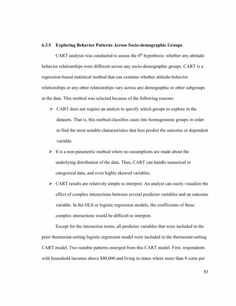
83

6.3.5 Exploring Behavior Patterns Across Socio-demographic Groups

CART analysis was conducted to assess the 4th hypothesis: whether any attitude-

behavior relationships were different across any socio-demographic groups. CART is a

regression-based statistical method that can examine whether attitude-behavior

relationships or any other relationships vary across any demographic or other subgroups

in the data. This method was selected because of the following reasons:

� CART does not require an analyst to specify which groups to explore in the

datasets. That is, this method classifies cases into homogeneous groups in order

to find the most notable characteristics that best predict the outcome or dependent

variable.

� It is a non-parametric method where no assumptions are made about the

underlying distribution of the data. Thus, CART can handle numerical or

categorical data, and even highly skewed variables.

� CART results are relatively simple to interpret. An analyst can easily visualize the

effect of complex interactions between several predictor variables and an outcome

variable. In the OLS or logistic regression models, the coefficients of these

complex interactions would be difficult to interpret.

Except for the interaction terms, all predictor variables that were included in the

prior thermostat-setting logistic regression model were included in the thermostat-setting

CART model. Two notable patterns emerged from this CART model. First, respondents

with household incomes above $40,000 and living in states where more than 8 cents per

84

capita was spent on energy efficiency programs were the most likely group to report

changing thermostat settings to save energy (see Figure 14). Second, respondents who

had household incomes below $40,000 and greater concern about energy use in the U.S.

society were the second most likely group to report changing thermostat settings to save

energy (see Figure 14). These results show that attitude-behavior relationships vary

across certain income groups.

Figure 14: CART Result (Pooled 2002-2006 National Data)

Note: Only those with access to a thermostat were included in this analysis.

Further analysis revealed that more than one-quarter (25% in 2002, 29% in 2004,

and 41% in 2006) of households with lower incomes (less than $40,000 a year) were 65

years old or older and likely retired, whereas about one-tenth (10% in 2002, 9% in 2004,

and 13% in 2006) of those with higher incomes (more than $40,000 a year) were 65 years

old or older. From prior research, it is known that older adults are less likely to change

Thermostat-settingBehavior

92% (n=846)

Thermostat-setting Behavior 87% (n=1887)




82% (n=128)

$/capita spent on EE programs in the state of residence is more than 0.08

$/capita spent on EE programs in the state of residence is less than 0.08

Household income is less than $40,000 a year

Household income is more than $40,000 a year


81% (n=627)


90% (n=286)

Lower concern about energy use in the U.S. society (average rating on items denoting this attitude is less than 4)

Higher concern about energy use in the U.S. society (average rating on items denoting this attitude is more than 4)

85

thermostat settings than younger adults due to health concerns (Peters, 1989). This may

explain why in the 2002, 2004, and 2006 samples it is observed that lower-income

households (an older group) compared to higher-income households (a younger group)

are less likely to report changing thermostat settings to save energy.

6.3.6 Summary

The thermostat-setting behavior analyses discussed in Section 6 revealed three

important patterns. First, lack of access to a thermostat was a key obstacle to being

engaged in a thermostat-setting behavior. About one-quarter of respondents reported no

access to a thermostat in their homes in the 2002, 2004, and 2006 samples. Among those

who had access to a thermostat, the vast majority (84-90%) reported changing their

thermostat setting to save energy.

Second, those more concerned about the environment were more likely to change

their thermostats to save energy than those less concerned about the environment. There

was a positive and significant relationship between the pro-environmental attitude and

thermostat-setting behavior. This relationship remained significant when controlling for

time and various demographic and external factors.

Third, there was no clear evidence that budget or other socio-demographic factors

moderated any of the attitude-behavior relationships explored in the preceding sections.

Although CART analysis did show that respondents who had household incomes below

$40,000 and high concern about energy use in the U.S. society were the second most

likely group (after those with household incomes above $40,000) to report changing

thermostat settings to save energy, income-attitude interaction terms in the logistic

86

regression models were not significant. Similarly, other attitude-socio-demographic

interaction terms in the logistic regression models were not significant.

6.4 Attitudes and CFL Installation Behavior

This section discusses notable findings from descriptive and OLS regression

analyses that explored the associations among the two attitudes referenced above, CFL

installation behavior, and several additional situational and external variables.


The 2004 to 2010 datasets were combined into one dataset.18 Initial analysis of

these pooled data revealed that the pro-environmental attitude and the attitude about

societal energy use had a significant and moderate correlation (r =.48). All other

significant correlations noted in Table 23 were weak.

18 In 2002, respondents were not asked how many CFL bulbs they had in their homes. For this reason, the

2002 data were excluded from this and subsequent OLS regression analysess.

87

Table 23

Correlations Among Attitudes, Behavior, and Time (Pooled 2004-2010 Data)

Pro-environmental

Attitude


Energy Use

CFL Installation Behavior (# of

CFLs in the home) .07** .01

Time 1: 2004 (2004=1, 2006=0, 2008=0, 2010=0)

-.01 -.04

Time 2: 2006 (2004=0, 2006=1, 2008=0, 2010=0)

-.02 -.03

Time 3: 2008 (2004=0, 2006=0, 2008=1, 2010=0)

.04 .05**

Attitude About Soc. Energy Use .48** --


Note: All missing data were imputed by using the Multiple Imputation method. For details on how the

imputation was done, see Section 5.2.1 and Appendix B.

6.4.2 Modeling Attitudinal Effect on CFL Installation Behavior

The OLS regression analyses were conducted to test whether attitudes explored in

this study are positively associated with CFL installation behavior (1st hypothesis), and

whether any attitudinal effects on this behavior persist over time (2nd hypothesis). To test

these hypotheses, associations between the CFL installation behavior (i.e., self-report of

the number of CFLs in the home) and attitudes toward the environment and energy use in

the U.S. society were explored together with several important demographic and external

factors that may have an effect on whether residents installed CFL bulbs in their homes.

For each OLS regression model, presented in this and subsequent sections, the Breusch-

Pagan test was conducted to check for heteroscedasticity. The test showed

heteroscedasticity was an issue. To address this issue, the robust standard errors were

estimated for each OLS regression model.

88

The first OLS regression model examined the attitude-behavior relationships,

while controlling for time. Table 24 displays the results (the unstandardized and

standardized coefficients). Results show that for each unit increase in the pro-

environmental score, the respondent reported having more than one additional CFL bulb

in the home; and for each unit increase in the score denoting concern about energy use in

the U.S. society, the respondent reported having fewer CFL bulbs in the home (see Table

24). Results also show that those in 2004 and 2006 were significantly less likely than

those in the 2010 study to have additional CFL bulbs in their home. This model, shown in

Table 24, explained a small amount of variance; R² value was 0.10. The overall model fit

was significant (F=69.4, p<0.05).

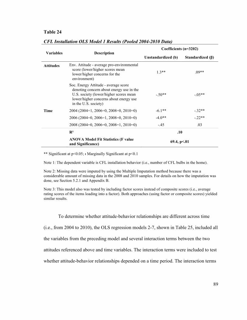
89

Table 24

CFL Installation OLS Model 1 Results (Pooled 2004-2010 Data)

Variables Description Coefficients (n=3202)

Unstandardized (b) Standardized (β)


1.3** .09**


-.50** -.05**

Time 2004 (2004=1, 2006=0, 2008=0, 2010=0) -6.1** -.32**

2006 (2004=0, 2006=1, 2008=0, 2010=0) -4.0** -.22**

2008 (2004=0, 2006=0, 2008=1, 2010=0) -.45 .03

R² .10

ANOVA Model Fit Statistics (F value

and Significance) 69.4, p<.01


Note 1: The dependent variable is CFL installation behavior (i.e., number of CFL bulbs in the home).

Note 2: Missing data were imputed by using the Multiple Imputation method because there was a considerable amount of missing data in the 2008 and 2010 samples. For details on how the imputation was

done, see Section 5.2.1 and Appendix B.

Note 3: This model also was tested by including factor scores instead of composite scores (i.e., average rating scores of the items loading into a factor). Both approaches (using factor or composite scores) yielded

similar results.

To determine whether attitude-behavior relationships are different across time

(i.e., from 2004 to 2010), the OLS regression models 2-7, shown in Table 25, included all

the variables from the preceding model and several interaction terms between the two

attitudes referenced above and time variables. The interaction terms were included to test

whether attitude-behavior relationships depended on a time period. The interaction terms

90

were constructed by multiplying attitudinal variables and time variables. There were no

significant interactions (see Table 25).

91

Table 25

CFL Installation OLS Model 2-7 Results (Pooled 2004-2010 Data)


Standardized Coefficients (n=3202)

Model

2

Model

3

Model

4

Model

5

Model

6

Model

7


.11** .09** .08** .09** .09** .09**


-.05** -.05** -.05** -.05** -.05** -.06**

Time 2004 (2004=1, 2006=0, 2008=0, 2010=0)

-.12 -.31** -.31** -.28** -.31** -.31**

2006 (2004=0, 2006=1, 2008=0, 2010=0)

-.23** -.24** -.23** -.23** -.21** -.23**

2008 (2004=0, 2006=0, 2008=1, 2010=0)

-.03 -.03 -.20 -.03 -.03 -.09

Interacti-

ons

Env. Attitude * 2004 -.19 -- -- -- -- --

Env. Attitude * 2006 -- .01 -- -- -- --

Env. Attitude * 2008 -- -- .17 -- -- --

Soc. Energy Attitude * 2004 -- -- -- -.03 -- --

Soc. Energy Attitude * 2006 -- -- -- -- -.02 --

Soc. Energy Attitude * 2008 -- -- -- -- -- .06

R² .10 .10 .10 .10 .10 .10

ANOVA Model Fit Statistics (F

value and Significance)

58.2,

p<.01

57.7,

p<.01

58.1,

p<.01

57.7,

p<.01

57.7,

p<.01

57.8,

p<.01





Note 3: This model also was tested by including factor scores instead of composite scores (i.e., average rating scores of the items loading into a factor). Both approaches (using factor or composite scores) yielded

similar results.

92

To assess how the CFL installation behavior would vary with a percent change in

the attitude score, the elasticity of the environmental attitude was calculated using the

environmental attitude regression coefficient from Model 1.19 Elasticity is an indicator of

how responsive one variable is to a change in another. The elasticity was 0.55. This

means that one percentage point increase on the attitude scale would increase the

adoption of CFL installation behavior by about half a percentage point. Alternatively, ten

percentage point increase on the attitude scale would increase the adoption of CFL

installation behavior by about five percentage points.

Because it is known that external conditions, house structure, and household

characteristics also can affect residential energy use, the next OLS regression model

explored attitude-behavior relationships while controlling for time and several external

and demographic factors. The aim was to test if any significant attitude-behavior

relationships remained significant when controlling for external and demographic

characteristics. Figure 15 lists which important external and demographic variables were

included in the next OLS regression model (Model 8).

19 The elasticity was computed by multiplying the env. attitude regression coefficient from Model 1 with the env.attitude mean value divided by the # of CFLs, estimated by using the regression equation from

Model 1.

93


Behavior Identified From the Literature Review

In red are variables present in the data and included in the subsequent regression models.

In Model 8, eight variables were significant: the environmental attitude,

household income, home ownership, house type, number of occupants, awareness of the

ENERGY STAR label, and two time variables (see Table 26). One variable was

marginally significant: dollars spent per capita on energy efficiency programs in the state

of residence (see Table 26). With respect to attitudes, these findings demonstrate that the

environmental attitude (an attitude that was significant in the prior models) remained

significant when controlling for external and demographic factors. The overall model fit

Individual

1. Perceptions about: conservation, comfort, social norms, and perceived costs (Limited data; examining only two conservation-related attitudes: concern for the environment and concern for energy use in the U.S. society)

2. Age

3. Pertinent Knowledge (Limited data; have data only on awareness of ENERGY STAR label)

Environment

Structure


2. Home age



External


2. Energy/product prices (Included electricity price data)

3. Energy efficiency (EE) programs (Included data on $ spent per capita on EE programs in the state of residence)

4. Building codes and appliance standards (No data, but included region, since these factors vary by region)

Households


2. Home owners


4. Income


94

was significant (F=29.3, p<0.05) and the model explained a small amount of variance

(R²=0.16).

Two additional CFL installation models were examined: Model 8a and 8b (see

Appendix E). These two models included the same variables as in Model 8 but examined

only those who adopted CFLs. In Model 8b, a log transformation of the dependent

variable was performed (to assess if transformed data could give a better fit), while in

Model 8a, the dependent variable was not transformed in any way. The results from these

two models were similar to the results in Model 8 (the same variables were significant;

see Appendix E). In terms of the overall fit, the model where log transformation of the

CFL installation variable was performed explained a greater amount of variance

(R²=0.17) than the model where log transformation of the CFL installation variable was

not performed (R²=0.11).

95

Table 26

CFL Installation OLS Model 8 Results (Pooled 2004-2010 Data)


Std.

Coefficients

(n=3202)


.07**


-.02

Economic

Consider-

ations

Household Income (Categories: 1=less than $20k to 8=more than $80k) .10**


-.003


.002

House and

Household

Attributes

Home Ownership (1=Own, 0=Rent) .05**

House Type (1=Single-family Home, 0=Other) .04**

Number of people living in the home .10**

Age of Respondent (Years) .02




Energy

and

Product

Prices

Average Retail Price of Electricity (cents/kWh) in the state of residence .02

Price of CFL bulb in the region of residence ($/CFL) .01

Weather Number of Heating Degree Days (HDDs) in the state of residence .03

Energy

Efficiency

Funding


.05ᵻ

Knowledge Awareness of ENERGY STAR label (1=Yes, 0=No) .10**

Time 2004 (2004=1, 2006=0, 2008=0, 2010=0) -.26**

2006 (2004=0, 2006=1, 2008=0, 2010=0) -.19**

2008 (2004=0, 2006=0, 2008=1, 2010=0) -.004

R² .16

ANOVA Model Fit Statistics (F value and Significance) 29.3, p<.01


Note 1: Dependent variable is CFL installation behavior (i.e., number of CFL bulbs in the home).

96



Note 3: Respondents reported their zip codes. Zip codes were used to link the average state-level retail

price of electricity with each case in the dataset.

Note 4: This model also was tested by including factor scores instead of composite scores (i.e., average

rating scores of the attitudinal items). Using factor scores yielded similar results.

The next model, Model 9, examined whether those who had never adopted CFLs

were different from those who had adopted CFLs. The aim was to test whether significant

variables in the prior OLS regression model, Model 8, were also significant in this

logistic regression model. The results show two notable differences between this logistic

and the prior OLS regression model: (1) Home ownership, a significant predictor in the

prior OLS regression model, was not significant in the logistic regression; and (2) Age, a

non-significant predictor in the prior OLS regression model, was significant in the

logistic regression model (see Table 26 and Table 27). These findings suggest that those

not adopting any CFLs were different in age than those adopting CFLs and home

ownership only differentiated among those who adopted CFLs.

97

Table 27

CFL Installation Logistic Model 9 Results (Pooled 2004-2010 Data)


(n=3202)


1.4**


.96

Economic

Consider-

ations

Household Income (Categories: 1=less than $20k to 8=more than $80k) 1.1**

I worry that the cost of energy for my home will increase (5-pt scale from 1=strongly disagree - 5=strongly agree)

1.0


.99

House and

Household

Attributes

Home Ownership (1=Own, 0=Rent) 1.1

House Type (1=Single-family Home, 0=Other) 1.2ᵻ

Number of people living in the home 1.1**

Age of Respondent (Years) 1.01**

Region Reside in the Midwest (Northeast=0, Midwest=1, South=0, West=0) 1.3

Reside in the South (Northeast=0, Midwest=0, South=1, West=0) 1.4

Reside in the West (Northeast=0, Midwest=0, South=0, West=1) 1.5

Energy

and

Product

Prices

Average Retail Price of Electricity (cents/kWh) in the state of residence 1.0


Weather Number of Heating Degree Days (HDDs) in the state of residence 1.0

Energy

Efficiency

Funding


1.02**

Knowledge Awareness of ENERGY STAR Label (1=Yes, 0=No) 1.7**

Time 2004 (2004=1, 2006=0, 2008=0, 2010=0) .36**

2006 (2004=0, 2006=1, 2008=0, 2010=0) .55**

2008 (2004=0, 2006=0, 2008=1, 2010=0) 1.1




Note 1: The dependent variable is CFL installation behavior (Binary variable where 0=No CFLs and 1=Have at least one CFL in the home).

98




price of electricity with each case in the dataset.

Note 4: This model also was tested by running this model as a probit model. The probit model had similar

results.


This section discusses notable results from the OLS regression analyses, which


It is hypothesized (3rd hypothesis) that budget moderates attitude-behavior relationships.

To assess this hypothesis, the following steps were executed: (1) multiplied household

income and environmental attitude, (2) multiplied household income and societal energy-

use attitude, and (3) added these two interaction terms to the OLS regression models

(Model 10 and 11), while controlling for all those other variables from the preceding

model – Model 8.

In terms of main effects, in Model 10, six variables were significant: home

ownership, house type (single-family versus non-single-family home), number of

occupants, awareness of ENERGY STAR label, and two time variables (see Table 28). In

Model 11, seven variables were significant: the environmental attitude, home ownership,

house type (single-family versus non-single-family home), number of occupants,

awareness of ENERGY STAR label, and two time variables (see Table 28). In both

Model 10 and 11, one variable was marginally significant: dollars spent per capita on

energy efficiency programs in the state of residence (see Table 28). The overall OLS

99

regression model explained a small amount of variance. In both models, the R² value was

0.16 and the overall model fit was significant (see Table 28).

In terms of interaction effects, only the household income and pro-environmental

attitude interaction was significant (see Table 28).

100

Table 28

CFL Installation OLS Models with Income-Attitude Interactions (Pooled 2004-2010

Data)


Std. Coefficients

(n=3202)

Model

10

Model

11


.004 .07**


-.02 -.05ᵻ

Economic

Considera-

tions


-.13 .03


-.003 -.004


.004 .003

House and

Household

Attributes

Home Ownership (1=Own, 0=Rent) .05** .05**

House Type (1=Single-family Home, 0=Other) .04** .04**

Number of people living in the home .10** .10**

Age of Respondent (Years) .02 .02

Region Reside in the Midwest (Northeast=0, Midwest=1, South=0, West=0)

.04 .04


.02 .03


.04 .05

Energy and

Product

Prices

Average Retail Price of Electricity (cents/kWh) in the state of residence .02 .01

Price of CFL bulb in the region of residence ($/CFL) .01 .01

Weather Number of Heating Degree Days (HDDs) in the state of residence

.03 .02

Energy

Efficiency

Funding


.05ᵻ .05ᵻ

Knowledge Awareness of ENERGY STAR Label (1=Yes, 0=No) .10** .10**

Time 2004 (2004=1, 2006=0, 2008=0, 2010=0) -.24** -.24**

2006 (2004=0, 2006=1, 2008=0, 2010=0) -.18** -.18**

2008 (2004=0, 2006=0, 2008=1, 2010=0) -.003 -.003

Interactions Env. Attitude * Household Income .24** --

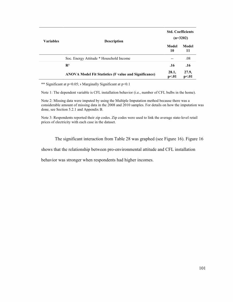
101


Std. Coefficients

(n=3202)

Model

10

Model

11

Soc. Energy Attitude * Household Income -- .08

R² .16 .16

ANOVA Model Fit Statistics (F value and Significance)

28.1,

p<.01

27.9,

p<.01






prices of electricity with each case in the dataset.

The significant interaction from Table 28 was graphed (see Figure 16). Figure 16

shows that the relationship between pro-environmental attitude and CFL installation

behavior was stronger when respondents had higher incomes.

102

Figure 16: Visualizing the Marginally Significant Interaction from Table 28


To test whether other situational variables, besides income, moderate attitude-

behavior relationship, several interaction terms were created by multiplying the two

attitudinal variables by those situational and external variables present in the databases:

(1) home ownership (if respondent owns or rents the residence), (2) respondent’s age, (3)

household size (# of people living in the home), (4) house type (if single-family detached

or other type of home), (5) average retail price of electricity in the state of residence, (6)

average prices of CFL bulbs in the state of residence, (7) number of HDDs in the state of

103

residence, and (8) dollars per capita spent on energy efficiency programs in the state of

residence.

No significant interactions were observed, as noted in Table 29. The overall OLS

models (Model 12-27) explained a small amount of variance; R² values were 0.16 in all

models. The overall model fit was significant for all models (see Table 29).

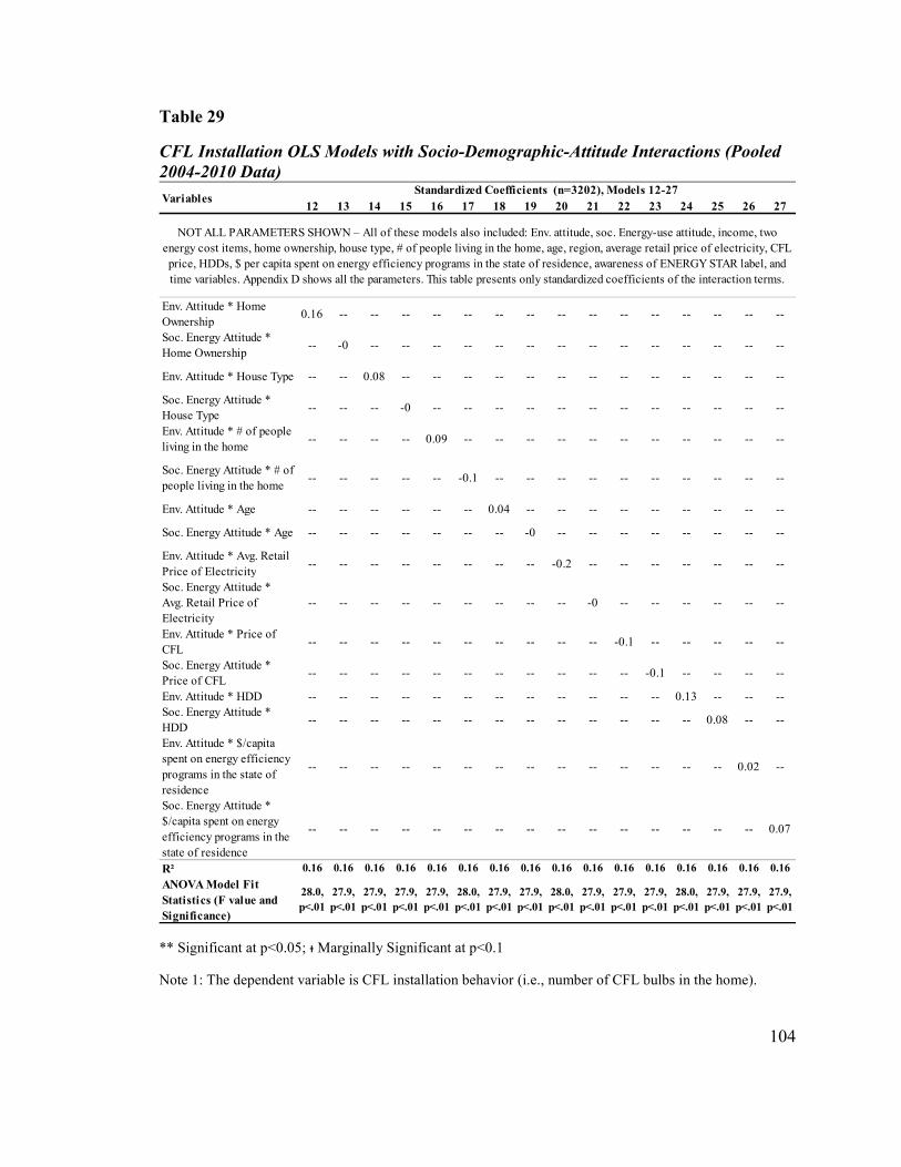
104

Table 29

CFL Installation OLS Models with Socio-Demographic-Attitude Interactions (Pooled

2004-2010 Data)



12 13 14 15 16 17 18 19 20 21 22 23 24 25 26 27

Env. Attitude * Home

Ownership0.16 -- -- -- -- -- -- -- -- -- -- -- -- -- -- --

Soc. Energy Attitude *

Home Ownership-- -0 -- -- -- -- -- -- -- -- -- -- -- -- -- --

Env. Attitude * House Type -- -- 0.08 -- -- -- -- -- -- -- -- -- -- -- -- --


House Type-- -- -- -0 -- -- -- -- -- -- -- -- -- -- -- --

Env. Attitude * # of people

living in the home-- -- -- -- 0.09 -- -- -- -- -- -- -- -- -- -- --

Soc. Energy Attitude * # of

people living in the home-- -- -- -- -- -0.1 -- -- -- -- -- -- -- -- -- --

Env. Attitude * Age -- -- -- -- -- -- 0.04 -- -- -- -- -- -- -- -- --

Soc. Energy Attitude * Age -- -- -- -- -- -- -- -0 -- -- -- -- -- -- -- --

Env. Attitude * Avg. Retail

Price of Electricity-- -- -- -- -- -- -- -- -0.2 -- -- -- -- -- -- --


Avg. Retail Price of

Electricity

-- -- -- -- -- -- -- -- -- -0 -- -- -- -- -- --

Env. Attitude * Price of

CFL-- -- -- -- -- -- -- -- -- -- -0.1 -- -- -- -- --


Price of CFL-- -- -- -- -- -- -- -- -- -- -- -0.1 -- -- -- --

Env. Attitude * HDD -- -- -- -- -- -- -- -- -- -- -- -- 0.13 -- -- --


HDD-- -- -- -- -- -- -- -- -- -- -- -- -- 0.08 -- --

Env. Attitude * $/capita

spent on energy efficiency

programs in the state of

residence

-- -- -- -- -- -- -- -- -- -- -- -- -- -- 0.02 --


$/capita spent on energy

efficiency programs in the

state of residence

-- -- -- -- -- -- -- -- -- -- -- -- -- -- -- 0.07

R² 0.16 0.16 0.16 0.16 0.16 0.16 0.16 0.16 0.16 0.16 0.16 0.16 0.16 0.16 0.16 0.16

ANOVA Model Fit

Statistics (F value and

Significance)

28.0,

p<.01

27.9,

p<.01

27.9,

p<.01

27.9,

p<.01

27.9,

p<.01

28.0,

p<.01

27.9,

p<.01

27.9,

p<.01

28.0,

p<.01

27.9,

p<.01

27.9,

p<.01

27.9,

p<.01

28.0,

p<.01

27.9,

p<.01

27.9,

p<.01

27.9,

p<.01

VariablesStandardized Coefficients (n=3202), Models 12-27

NOT ALL PARAMETERS SHOWN – All of these models also included: Env. attitude, soc. Energy-use attitude, income, two

energy cost items, home ownership, house type, # of people living in the home, age, region, average retail price of electricity, CFL

price, HDDs, $ per capita spent on energy efficiency programs in the state of residence, awareness of ENERGY STAR label, and

time variables. Appendix D shows all the parameters. This table presents only standardized coefficients of the interaction terms.

105




prices of electricity with each case in the dataset.

6.4.5 Exploring Behavior Patterns Across Socio-Demographic Groups

CART analysis was conducted to assess the 4th hypothesis: whether any attitude-

behavior relationships are different across any socio-demographic groups.


prior CFL installation OLS model were included in the CFL installation CART model.

Several notable patterns emerged from this CART model. First, respondents who were

surveyed in 2004 had the smallest number of CFLs in their homes, on average. Second,

the group with the greatest number of CFLs in their homes were those who took the

survey in later years (2008 and 2010), had incomes above $40,000, and were aware of the

ENERGY STAR label (see Figure 17). Third, there was one common pattern among the

groups with the smallest and the greatest number of CFLs in the home: those aware of the

ENERGY STAR label in each group had more CFLs in the home than those not aware of

this label (see Figure 17). These findings demonstrate that there are complex

relationships between time and other non-attitudinal variables.

106

Figure 17: CART Result (Pooled 2004-2010 National Data)

6.4.6 Summary

The CFL analyses discussed in Section 6 revealed four important patterns. First,

adoption of CFL bulbs among respondents increased substantially over time. The

percentage of those who installed more than one CFL bulb increased from 42% in 2004

to 76% in 2010. OLS analyses confirmed that this CFL adoption pattern was significant

and notable.

Second, those more concerned about the environment were more likely to have

more CFLs in their home than those less concerned about the environment. There was a

107

positive and significant relationship between the pro-environmental attitude and CFL

installation behavior. This relationship remained significant when controlling for time

and various demographic and external factors.

Third, there is evidence that budget moderated the relationship between the pro-

environmental attitude and CFL installation behavior (a pattern not seen with the

thermostat-setting behavior). The interaction between income and the pro-environmental

attitude was positive and significant in the OLS regression model, which indicated that

the relationship between the pro-environmental attitude and CFL installation behavior

was stronger when respondents had higher incomes.

Fourth, complex relationships existed between time and non-attitudinal variables,

and CFL installation behavior. CART analysis revealed that the group with the greatest

number of CFLs in their homes took the survey in later years (2008 and 2010), had

incomes above $40,000, and were aware of ENERGY STAR label.

108

7. FINDINGS FROM THE CALIFORNIA DATASET

Researchers at Abt SRBI and Research Into Action conducted another survey

about energy attitudes and behaviors in the State of California. This dataset was

examined as well. Specifically, the focus of this analysis was two-fold: (1) to assess

whether any attitude-behavior patterns in this dataset were similar to those observed in

the national datasets, and (2) to assess whether any attitude-behavior relationships were

different across regions that were determined to be politically more conservative or

liberal (see Section 7.4 for more details). The regional analysis was reasonable because

the dominant political ideology of an area may influence residents’ attitudes regarding

energy use.

7.1 Assessment of Attitudinal Items


California residents who agreed to take the survey rated how much they agreed

with the energy-related statements listed in Table 30, using a scale from 1 to 5 where 1

meant “strongly disagree,” “no impact,” or “not at all convinced” and 5 meant “strongly

agree,” “significant impact,” or “completely convinced.” Table 30 displays the average

ratings of the 13 attitudinal statements. Frequencies of these responses are displayed in

Appendix A.

109

Table 30

Thirteen Attitudinal Statements (Means)

Respondents rated the following statements from 1=strongly disagree to 5=strongly

agree (unless noted otherwise) 2010 (n=2000)

General environmental statements

1. I’m very concerned about the environment. 4.1

2. I look for products that are good for the environment. 4.0

3. Saving energy helps the environment. 4.3

4. Making my home energy-efficient is good for the environment. (7-pt scale where 1=strongly disagree and 7=strongly agree)

5.9

Global warming statements

5. Global warming is a result of high energy use. 3.3

6. People should try to use less energy to reduce global warming. 3.8

7. How convinced are you that global warming is happening - would you say not at all, not too convinced, somewhat, mostly, or completely convinced?

3.5

8. On a scale of 1 to 5 where 1 is “no impact” and 5 is “a very significant impact,” to what extent do you believe your actions have an impact on the rate or speed of global warming?

3.0


9. Saving energy in the home helps me save money. 4.4

10. The cost of energy makes me want to conserve. 4.2

11. I sometimes worry whether there is enough money to pay my energy bill. 2.8


12. I've already done everything I can to save energy in my home. 3.3

13. I’m too busy to be concerned with saving energy in my home. 2.0

Note: Means reported in this table are estimated using the Full Maximum Likelihood (FIML) missing data estimation. There were no notable differences in estimations of the means when using listwise deletion

compared to FIML missing data estimation.

7.1.2 Cronbach's Alpha

Cronbach's alpha analysis was the first step in identifying latent variables or

highly correlated items that represent a larger attitudinal construct. Specifically,

Cronbach's alpha was used to check for internal consistency or reliability between the

attitudinal items in this dataset. The global warming and general environmental items,

110

listed in Table 31, had the highest and second highest Cronbach's alpha values (.83 and

.71, respectively). All other Cronbach's alpha values were below 0.6. Generally, values of

0.70 or higher are acceptable indicators of reliability. Deleting items, when possible,

improved Cronbach's alpha values for “cost of energy” items only (see Table 31). This

improvement was not large enough to indicate that those items reliably measured a larger

attitudinal construct.

111

Table 31

Cronbach’s Alpha Reliability Coefficients

Respondents rated the following statements from 1=Strongly

Disagree to 5=Strongly Agree (unless noted otherwise)

2010 (n=2000)

Cronbach’s

Alpha

Cronbach’s Alpha

if Item Deleted

General environmental statements

1. I’m very concerned about the environment. .71 If items 1, 2, or 3

are deleted,

Cronbach’s alpha

value decreases

If item 4 is

deleted,

Cronbach’s alpha

value remains at

.71



4. Making my home energy-efficient is good for the environment. (7-pt scale where 1=strongly disagree and 7=strongly agree)

Because item “4” had a different scale than items “1-3,” Z-scores

were computed for all four items and used to calculate the

Cronbach’s alpha value.

Global warming statements

5. Global warming is a result of high energy use.

.83

If any of the 5-8

items are deleted,

Cronbach’s alpha

value decreases

6. People should try to use less energy to reduce global warming.

7. How convinced are you that global warming is happening - would you say not at all, not too convinced, somewhat, mostly, or completely convinced?

8. On a scale of 1 to 5 where 1 is “no impact” and 5 is “a very significant impact,” to what extent do you believe your actions have an impact on the rate or speed of global warming?


9. Saving energy in the home helps me save money.

.47

If item 11 is

deleted,

Cronbach’s alpha

value increases to

.56

10. The cost of energy makes me want to conserve.



12. I've already done everything I can to save energy in my home. .02 -


Note: Missing data were imputed by using the Multiple Imputation method. For details on how the imputation was done, see Section 5.2 and Appendix B.

112

7.1.3 CFA Results

Conducting the CFA was the second step in identifying latent variables or highly

correlated items that represent a larger attitudinal construct. Specifically, CFA was used

to test whether data fit a hypothesized two-factor structure inferred from the preceding

analysis. That is, whether global warming and general environmental items (those with

the highest and second highest Cronbach's alpha values) measured the pro-environmental

attitude and global warming attitude. Figure 8 displays the hypothesized two-factor CFA

model.

113

Figure 18: Hypothesized Two-factor Structure (2010 CA Data)

CFA results show that 2010 two-factor model had significant chi-square value

(see Table 32). Although a significant chi-square value indicates poor fit to the data, this

value is affected by the sample size (i.e., it is almost always statistically significant when

a sample size is large). Because of this limitation, the alternative fit indices were

examined to determine whether the two-factor model fit the data adequately. The

alternative fit indices suggested an acceptable fitting model. As shown in Table 32, CFI

was 0.99, RMSEA was .02, and SRMR was .06 (for CFI, a value close to one indicates a

good fitting model; for RMSEA and SRMR a value below 0.08 indicates a good fitting

114

model according to MacCallum, Browne, and Sugawara [1996]). A comparison of the

one-factor model and the two-factor model indicated that the two-factor model fit better

than the one-factor model. The two-factor model had a higher CFI and lower RMSEA

and SRMR values than the one-factor model.

Table 32

Goodness-of-Fit Indicators of Two-factor CFA Model (CA Data)

Model χ2(df) RMSEA SRMR CFI

2010 (n=2000) 30.7(19)** 0.02 0.06 0.99

**Significant at p<0.05

Note: Results reported in this table are estimated using the Full Maximum Likelihood (FIML) missing data

estimation.

The results also suggest that the four environmental items had significant

standardized loadings on the first factor (see Table 33). Similarly, the four items about

global warming had significant standardized loadings on the second factor (see Table 33).

Estimated correlation between the two factors was significant (p<0.05) and was 0.65.

115

Table 33

Unstandardized (Standardized) Loadings of Two-factor CFA Model (CA Data)

Statement 2010 (n=2000)

Saving energy helps the environment. 1.00 (.75)**

I’m very concerned about the environment. 1.37 (.89)**

I look for products that are good for the environment. 0.98 (.62)**

Making my home energy-efficient is good for the environment 1.69 (.48)**

Global warming is a result of high energy use. 1.00 (.79)**

People should try to use less energy to reduce global warming. 0.95 (.77)**

How convinced are you that global warming is happening - would you say not at all, not too convinced, somewhat, mostly, or completely convinced?

1.15 (.77)**

On a scale of 1 to 5 where 1 is “no impact” and 5 is “a very significant impact,” to what extent do you believe your actions have an impact on the rate or speed of global warming?

1.05 (.69)**

** Significant at p<0.05

Note: Results reported in this table are estimated using the Full Maximum Likelihood (FIML) missing data

estimation.

7.1.4 Attitudinal Measures

As noted in the preceding sections, Cronbach’s alpha values were above the

acceptable cutoff threshold for the general environmental items and global warming

items. The CFA results indicated that the standardized loadings for the general

environmental and global warming items were high and, overall, the CFA results

suggested the hypothesized two-factor model represented the data well. Based on these

findings, the respondents’ agreement ratings of the four general environmental statements

and four statements about global warming were averaged for each case in the dataset to

produce two attitudinal scores: (1) a score reflecting the respondent’s level of concern for

116

the environment in general, and (2) a score reflecting the respondent’s level of concern

about global warming. Lower scores indicate lower concerns for the environment or

global warming, whereas higher scores indicate higher concerns for the environment or

global warming.

Table 34

Mean Scores of the Two Attitudinal Measures (CA Data) 2010 (n=2000)

Pro-environmental score (average ratings of four general environmental statements; lower/higher scores mean lower/higher concerns for the environment)

4.6

Score reflecting how respondents think about global warming (average ratings of four statements about global warming; lower/higher scores mean lower/higher concerns about global warming)

3.4

Note: Missing data were imputed by using the Multiple Imputation method. For details on how the imputation was done, see Appendix B.

7.1.5 Items Excluded and Included in the Subsequent Analyses

Among thirteen attitudinal items shown in Table 30, only eight were combined to

create two attitudinal measures, as explained in the preceding sections. The rest of the

items (except two) were excluded from the subsequent analyses since it was unclear what

larger attitudinal or latent construct they measure. The items not combined to create an

attitudinal measure but included in the subsequent analyses were: "I sometimes worry

whether there is enough money to pay my energy bill" and “The cost of energy makes me

want to conserve.” These two items, together with income, contain information about the

respondent's economic situation, which is an important consideration when modeling

energy-use behavior. For this reason, these items were included in the subsequent

regression analyses as separate items and were not considered as attitudinal measures.

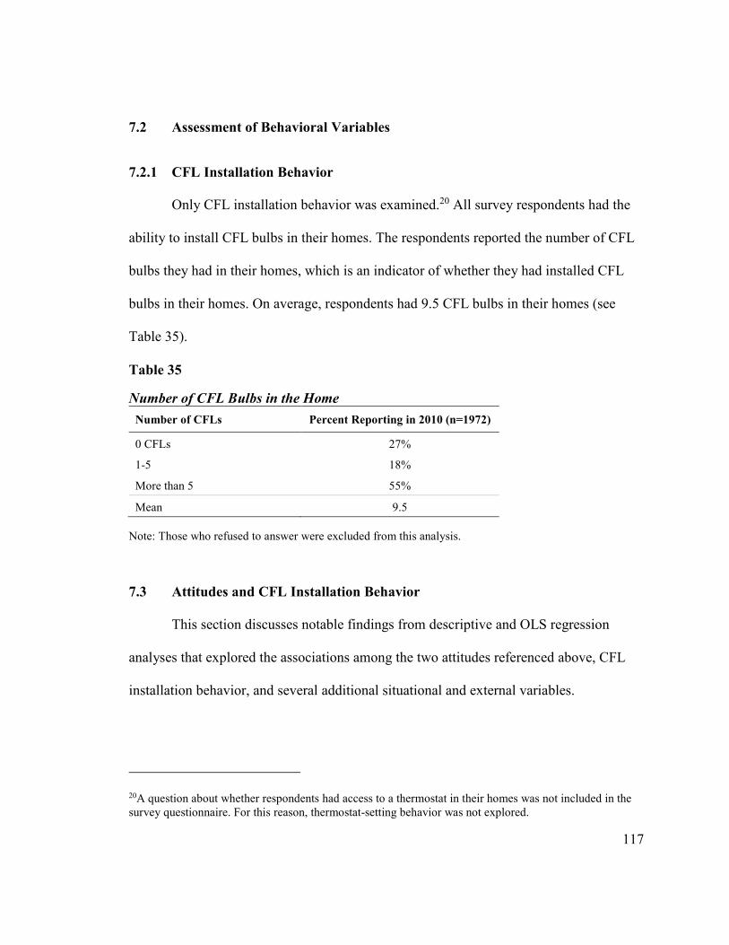
117

7.2 Assessment of Behavioral Variables

7.2.1 CFL Installation Behavior

Only CFL installation behavior was examined.20 All survey respondents had the

ability to install CFL bulbs in their homes. The respondents reported the number of CFL

bulbs they had in their homes, which is an indicator of whether they had installed CFL

bulbs in their homes. On average, respondents had 9.5 CFL bulbs in their homes (see

Table 35).

Table 35

Number of CFL Bulbs in the Home

Number of CFLs Percent Reporting in 2010 (n=1972)

0 CFLs 27%

1-5 18%

More than 5 55%

Mean 9.5


7.3 Attitudes and CFL Installation Behavior

This section discusses notable findings from descriptive and OLS regression

analyses that explored the associations among the two attitudes referenced above, CFL

installation behavior, and several additional situational and external variables.

20A question about whether respondents had access to a thermostat in their homes was not included in the

survey questionnaire. For this reason, thermostat-setting behavior was not explored.

118


Initial analysis of these data revealed that the general pro-environmental attitude

and the attitude about global warming had a significant and moderate correlation (r =.51).

All other significant correlations noted in Table 36 were weak.

Table 36

Correlations Between Attitudes and Behavior (2010 CA Data)

Attitude/Behavior Pro-environmental

Attitude

Attitude About Global

Warming

CFL installation behavior (# of CFLs in the home)

.10** .06**

Attitude about global warming .51** --


Note: All missing data were imputed by using the Multiple Imputation method because there was a considerable amount of missing data. For details on how the imputation was done, see Section 5.2.2 and Appendix B.

7.3.2 Modeling Attitudinal Effect on CFL Installation Behavior

The first OLS regression model examined the attitude-behavior relationships

while controlling for several external and demographic factors. The aim was to test

whether there were any significant attitude-behavior relationships when controlling for

the external and demographic characteristics listed in Figure 19. Figure 19 lists which

important external and demographic variables were included in the first OLS regression

model. For each OLS regression model, presented in this and subsequent sections, the

Breusch-Pagan test was conducted to check for heteroscedasticity. The test showed

119

heteroscedasticity was an issue. To address this issue, the robust standard errors were

estimated for each OLS regression model.


Behavior Identified from the Literature Review

In red are variables present in the data and included in the subsequent regression models.

Nine variables were significant: the environmental attitude, the global warming

attitude, household income, house type, number of occupants, whether respondent noted

any other race/ethnicity besides “white” or “Hispanic,” average monthly energy bill,

awareness of the ENERGY STAR label, and awareness of the carbon footprint concept

(see Table 37). Two variables were marginally significant: agreement with “the cost of

energy makes me want to conserve,” and agreement with “I sometimes worry whether

Individual

1. Perceptions about: conservation, comfort, social norms, and perceived costs (Limited data; examining only two conservation-related attitudes -- concern for the environment and global warming -- and whether comfort is perceived as an obstacle)

2. Age

3. Pertinent Knowledge (Limited data; have data only on awareness of ENERGY STAR label and carbon footprint concept)

Environment

Structure


2. Home age



External

1. Weather

2. Energy/product prices (Included self-reported average monthly energy bill)

3. Energy efficiency programs


Households


2. Home owners


4. Income


(Also included race)

120

there is enough money to pay my energy bill” (see Table 37). With respect to attitudes,

these findings demonstrate that the general environmental attitude and global warming

attitude (an attitude on a specific environmental topic) were significant when controlling

for external and demographic factors. The overall model fit was significant (F=14.3,

p<0.05) and the model explained a small amount of variance (R²=0.10).

Two additional CFL installation models were examined: Models 1a and 1b (see

Appendix E). These two models included the same variables as in Model 1 but examined

only those who adopted CFLs. In Model 1b, a log transformation of the dependent

variable was performed (to assess if transformed data could give a better fit), while in

Model 1a, the dependent variable was not transformed in any way. The results from these

two models differed from the results observed in Model 1. A fewer number of variables

were significant in Model 1a and 1b compared to Model 1 (see Table 37 and Appendix

E). The variables that were significant in Model 1a (household income, number of

occupants, and average monthly energy bill) also were significant in Model 1. In contrast,

not all variables that were significant in Model 1b were significant in Model 1.

Specifically, renters and Hispanics were significantly less likely to have more CFLs

among those who adopted CFLs, according to Model 1b, while home ownership and

being Hispanic were not significant variables in Model 1 (a model examining those who

had and had not adopted CFLs). In terms of the overall fit, Model 1b, for which log

transformation of the CFL installation variable was performed, explained a greater

amount of variance (R²=0.14) than Model 1a (R²=0.10).

121

Table 37

CFL Installation OLS Model 1 Results (2010 CA Data)

Variables Description Std. Coefficients

(n=2000)


.07**

Global Warming Attitude - average score denoting concern about global warming (lower/higher scores mean lower/higher concern)

.06**

Economic

Considerations


.09**

The cost of energy makes me want to conserve (5-pt scale from 1=strongly disagree to 5=strongly agree)

.03ᵻ


-.08ᵻ

Comfort Those who said desire for comfort is a barrier to saving energy at home (1= Said it, 0=Didn’t say it)

-.02

House and

Household

Attributes

Home Ownership (1=Own, 0=Rent) .02

House Type (1=Single-family Home, 0=Other) .04**


Age of Respondent (Years) -.02

Race (White=0, Hispanic=1, Other=0) -.04

Race (White=0, Hispanic=0, Other=1) -.04**

Region Northern/Southern CA (Northern=0, Southern=1) (Dividing line is the boundary between Monterey and San Luis Obispo)

-.01

Energy Price On average, how much is your monthly bill for all types of energy you use in your home, including electricity, natural gas, LPG, fuel oil, and any other fuels?. Your best estimate is fine. (Six categories: 1=Less than $50 to 6=More than $250)

.09**

Knowledge Awareness of ENERGY STAR Label (1=Yes, 0=No) .07**

Awareness of Carbon Footprint Concept (1=Yes, 0=No) .07**

R² .10




Note 2: Missing data were imputed by using the Multiple Imputation method. For details on how the imputation was done, see Section 5.2.2 and Appendix B.

Note 3: Respondents reported their zip codes. Zip codes were used to link the average state-level retail price of electricity with each case in the dataset.

122

The next model, Model 2, examined whether those who had never adopted CFLs

were different from those who had adopted CFLs. The aim was to test whether significant

variables in the prior OLS regression model, Model 1, also were significant in this

logistic regression model. The results showed that the following five significant

predictors in the prior OLS regression model were not significant in the logistic

regression model: the general environmental attitude, house type, number of occupants,

average monthly energy bill, and whether respondent noted any other race/ethnicity

besides “white” or “Hispanic” (see Table 37 and Table 38). These findings suggest that

these particular variables differentiated only among those who adopted CFLs.

123

Table 38

CFL Installation Logistic Model 2 Results (2010 CA Data)


(n=2000)


1.1


1.2**

Economic

Considerations


1.0**

The cost of energy makes me want to conserve (5-pt scale from 1=strongly disagree - 5=strongly agree)

1.1


.94


.85

House and

Household

Attributes


House Type (1=Single-family Home, 0=Other) 1.2

Number of people living in the home .97

Age of Respondent (Years) 1.0

Race (White=0, Hispanic=1, Other=0) .80

Race (White=0, Hispanic=0, Other=1) .92

Region Northern/Southern CA (Northern=0, Southern=1) (The dividing line is the boundary between Monterey and San Luis Obispo.)

1.1

Energy Price On average, how much is your monthly bill for all types of energy you use in your home, including electricity, natural gas, LPG, fuel oil, and any other fuels? Your best estimate is fine. (Six categories: 1=Less than $50 to 6=More than $250)

.85

Knowledge Awareness of ENERGY STAR Label (1=Yes, 0=No) 1.5**

Awareness of Carbon Footprint Concept (1=Yes, 0=No) 1.6**




Note 1: The dependent variable is CFL installation behavior (binary variable where 0=No CFLs and

1=Have at least one CFL in the home).

Note 2: Missing data were imputed by using the Multiple Imputation method. For details on how the


Note 3: This model also was tested as a probit model. The probit model had similar results.

124


This section discusses notable results from the OLS regression analyses, which


To assess these relationships, the following steps were executed: (1) multiplied household

income and general environmental attitude, (2) multiplied household income and global

warming attitude, and (3) added these two interaction terms to the OLS regression models

(Models 2 and 3), while controlling for all those other variables from the preceding

model – Model 1.

In terms of main effects, in Model 3, six variables were significant: the global

warming attitude, number of occupants, whether respondent noted any other

race/ethnicity besides “white” or “Hispanic,” average monthly energy bill, awareness of

the ENERGY STAR label, and awareness of the carbon footprint concept (see Table 39).

In Model 4, seven variables were significant: the environmental attitude, agreement with

the statement “the cost of energy makes me want to conserve,” number of occupants,

whether respondent noted any other race/ethnicity besides “white” or “Hispanic,” average

monthly energy bill, awareness of the ENERGY STAR label, and awareness of the term

“carbon footprint” (see Table 39). In both Model 3 and 4, two variables were marginally

significant: agreement with “I sometimes worry whether there is enough money to pay

my energy bill” and house type (see Table 39). The overall OLS regression model

explained a small amount of variance. In both models, the R² value was 0.11 and the

overall model fit was significant (see Table 39).

125

In terms of interaction effects, the household income and global warming attitude

interaction was significant (see Table 39). Similarly, the household income and the

general environmental attitude interaction was significant.

126

Table 39

CFL Installation OLS Models with Income-Attitude Interactions (2010 CA Data)


Std. Coefficients

(n=2000)

Model 3 Model 4


.01 .07**


.07** -.03

Economic

Consider-

ations


-.11 -.07


.03ᵻ .03**


-.09ᵻ -.09ᵻ


-.02 -.03

House and

Household

Attributes

Home Ownership (1=Own, 0=Rent) .02 .02

House Type (1=Single-family Home, 0=Other) .04ᵻ .04ᵻ

Number of people living in the home .06** .06**

Age of Respondent (Years) -.02 -.02

Race (White=0, Hispanic=1, Other=0) -.04 -.04

Race (White=0, Hispanic=0, Other=1) -.04** -.05**

Region Northern/Southern CA (Northern=0, Southern=1) (The dividing line is the boundary between Monterey and San Luis Obispo.)

-.01 -.01

Energy

Prices

On average, how much is your monthly bill for all types of energy you use in your home, including electricity, natural gas, LPG, fuel oil, and any other fuels? Your best estimate is fine. (Six categories: 1=Less than $50 to 6=More than $250)

.09** .09**

Knowledge Awareness of ENERGY STAR Label (1=Yes, 0=No) .07** .07**

Awareness of Carbon Footprint Concept (1=Yes, 0=No) .07** .07**

Interactions Env. Attitude *Household Income .21** --

Global Warming Attitude * Household Income -- .19**

R² .11 .11

ANOVA Model Fit Statistics (F value and Significance)

13.7,

p<.01

13.9,

p<.01



127



The significant interactions from Table 39 were graphed (see Figure 20 and

Figure 21). Figure 20 shows that the relationship between the global warming attitude

and CFL installation behavior was stronger when respondents had higher incomes.

Figure 21 shows that the relationship between the general environmental attitude and

CFL installation behavior also was stronger when respondents had higher incomes.

Figure 20: Visualizing the Significant Interactions From Table 39

128



To assess whether situational variables, other than income, moderate attitude-

behavior relationships, several interaction terms were created by multiplying the two

attitudinal variables with those situational and external variables present in the databases:

(1) home ownership (if respondent owns or rents the residence), (2) respondent’s age, (3)

household size (# of people living in the home), (4) house type (if single-family detached

or other type of home), (5) race, and (6) average monthly energy bill.

The average monthly energy bill and global warming attitude interaction was

significant (see Table 40). Similarly, the average monthly energy bill and the general

129

environmental attitude interaction was significant. The overall OLS models (Models 5-

18) explained a small amount of variance and the overall model fit was significant for all

models (see Table 40).

130

Table 40

CFL Installation OLS Models with Socio-Demographic-Attitude Interactions (2010 CA

Data)


Note 1: The dependent variable is CFL installation behavior (i.e., the number of CFL bulbs in the home).



5 6 7 8 9 10 11 12 13 14 15 16 17 18

Env. Attitude * Home

Ownership0.15 -- -- -- -- -- -- -- -- -- -- -- -- --

Global Warming

Attitude * Home

Ownership

-- 0.12 -- -- -- -- -- -- -- -- -- -- -- --

Env. Attitude *

House Type-- -- 0.11 -- -- -- -- -- -- -- -- -- -- --

Global Warming

Attitude * House

Type

-- -- -- 0.05 -- -- -- -- -- -- -- -- -- --

Env. Attitude * # of

people living in the

home

-- -- -- -- -0.08 -- -- -- -- -- -- -- -- --

Global Warming

Attitude * # of

people living in the

home

-- -- -- -- -- -0.06 -- -- -- -- -- -- -- --

Env. Attitude * Age -- -- -- -- -- -- 0.06 -- -- -- -- -- -- --

Global Warming

Attitude * Age-- -- -- -- -- -- -- 0.04 -- -- -- -- -- --

Env. Attitude * Race

(Hispanic)-- -- -- -- -- -- -- -- -0.06 -- -- -- -- --

Global Warming

Attitude * Race

(Hispanic)

-- -- -- -- -- -- -- -- -- -0.04 -- -- -- --

Env. Attitude * Race

(Other)-- -- -- -- -- -- -- -- -- -- -0.08 -- -- --

Global Warming

Attitude * Race

(Other)

-- -- -- -- -- -- -- -- -- -- -- -0.04 -- --

Env. Attitude * Avg.

Monthly Energy Bill-- -- -- -- -- -- -- -- -- -- -- -- .26** --

Global Warming

Attitude * Avg.

Monthly Energy Bill

-- -- -- -- -- -- -- -- -- -- -- -- -- .20**

R² 0.1 0.1 0.1 0.1 0.1 0.1 0.1 0.1 0.1 0.1 0.1 0.1 0.1 0.11

ANOVA Model Fit

Statistics (F value

and Significance)

13.6,

p<.01

13.6,

p<.01

13.5,

p<.01

13.5,

p<.01

13.5,

p<.01

13.5,

p<.01

13.5,

p<.01

13.5,

p<.01

13.5,

p<.01

13.5,

p<.01

13.5,

p<.01

13.5,

p<.01

13.8,

p<.01

14.0,

p<.01

VariablesStandardized Coefficients (n=2000), Models 5-18

NOT ALL PARAMETERS SHOWN – All of these models also included: Env. attitude, global warming attitude, income, two

energy cost items, home ownership, house type, # of people living in the home, age, region, average monthly energy bill, and

awareness of ENERGY STAR and carbon footprint. Appendix D shows all the parameters. This table presents only standardized

coefficients of the interaction terms.

131

The significant interactions from Table 40 were graphed (see Figure 22 and

Figure 23). Figure 22 shows that the relationship between the global warming attitude

and CFL installation behavior was stronger when respondents had larger monthly energy

expenditures or bills. Similarly, Figure 23 shows that the relationship between the general

environmental attitude and CFL installation behavior was stronger when respondents had

larger monthly energy expenditures or bills.

Figure 22: Visualizing the Significant Interactions from Table 40

132


7.3.5 Exploring Behavior Patterns Across Socio-demographic Groups

CART analysis was conducted to assess whether any attitude-behavior

relationships were different across any socio-demographic groups.


prior CFL installation OLS model were included in the CFL installation CART model. A

couple of notable patterns emerged from this CART model. First, respondents who were

unaware of the carbon footprint concept, had household incomes of less than $70,000 per

year, and were renters had the smallest number of CFLs in their homes, on average.

Second, those who were aware of the carbon footprint concept and had incomes above

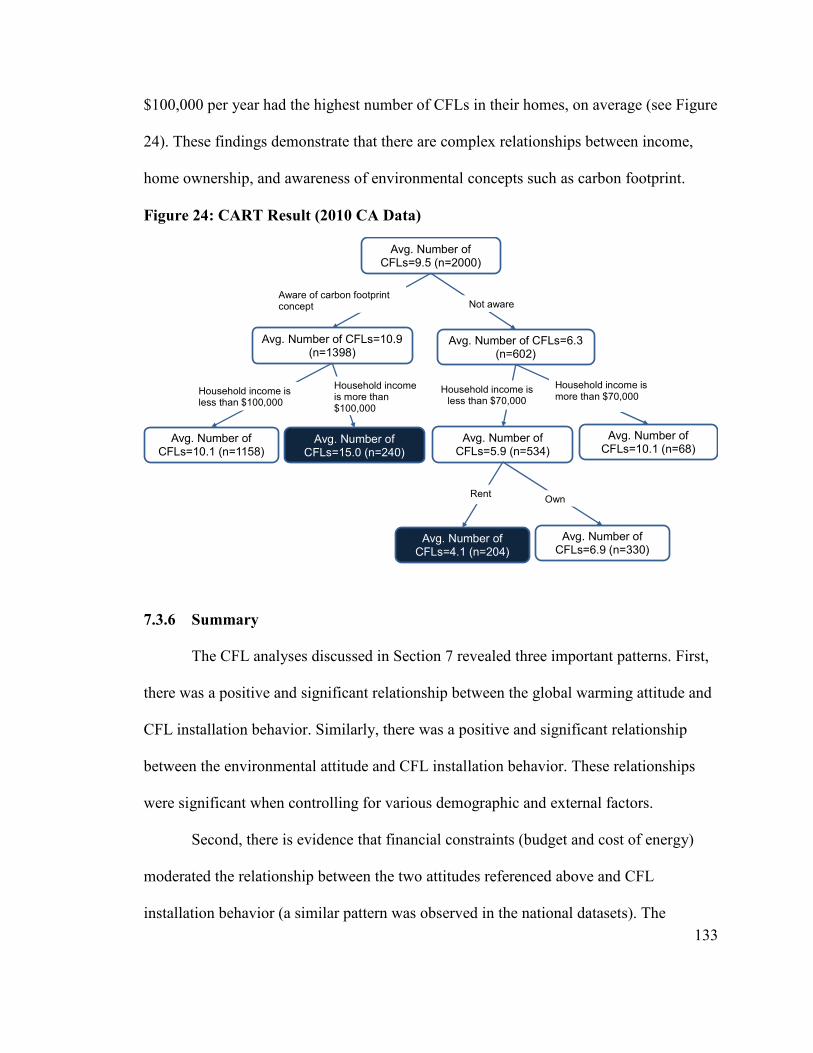
133

$100,000 per year had the highest number of CFLs in their homes, on average (see Figure

24). These findings demonstrate that there are complex relationships between income,

home ownership, and awareness of environmental concepts such as carbon footprint.

Figure 24: CART Result (2010 CA Data)

7.3.6 Summary

The CFL analyses discussed in Section 7 revealed three important patterns. First,

there was a positive and significant relationship between the global warming attitude and

CFL installation behavior. Similarly, there was a positive and significant relationship

between the environmental attitude and CFL installation behavior. These relationships

were significant when controlling for various demographic and external factors.

Second, there is evidence that financial constraints (budget and cost of energy)

moderated the relationship between the two attitudes referenced above and CFL

installation behavior (a similar pattern was observed in the national datasets). The

Avg. Number of CFLs=15.0 (n=240)

Household income is less than $100,000

Household incomeis more than $100,000






Not awareAware of carbon footprint concept

Household income is more than $70,000

Household income is less than $70,000




OwnRent

134

interactions between income and the global warming attitude and between average

monthly energy expenditures and the global warming attitude were positive and

significant in the OLS regression models, which indicated that the relationship between

the global warming attitude and CFL installation behavior was stronger when

respondents had higher incomes or greater monthly energy expenditures. Similarly, the

interactions between income and the general environmental attitude and between average

monthly energy expenditures and the general environmental attitude were positive and

significant in the OLS regression models, which indicated that the relationship between

the general environmental attitude and CFL installation behavior was stronger when

respondents had higher incomes or greater monthly energy expenditures.

Third, complex relationships existed between non-attitudinal variables and CFL

installation behavior. CART analysis revealed that respondents who were unaware of the

carbon footprint concept, had household incomes of less than $70,000 per year, and were

renters had the smallest number of CFLs in their homes, on average. Those who were

aware of the carbon footprint concept and had incomes above $100,000 per year had the

greatest number of CFLs in their homes, on average.

7.4 Regional Analyses

The following analyses focused on examining whether attitude-behavior

relationships were different across certain California regions while controlling for

relevant demographic and situational variables. Before executing this regional analysis,

respondents were classified into the six regional groups displayed in Table 41.

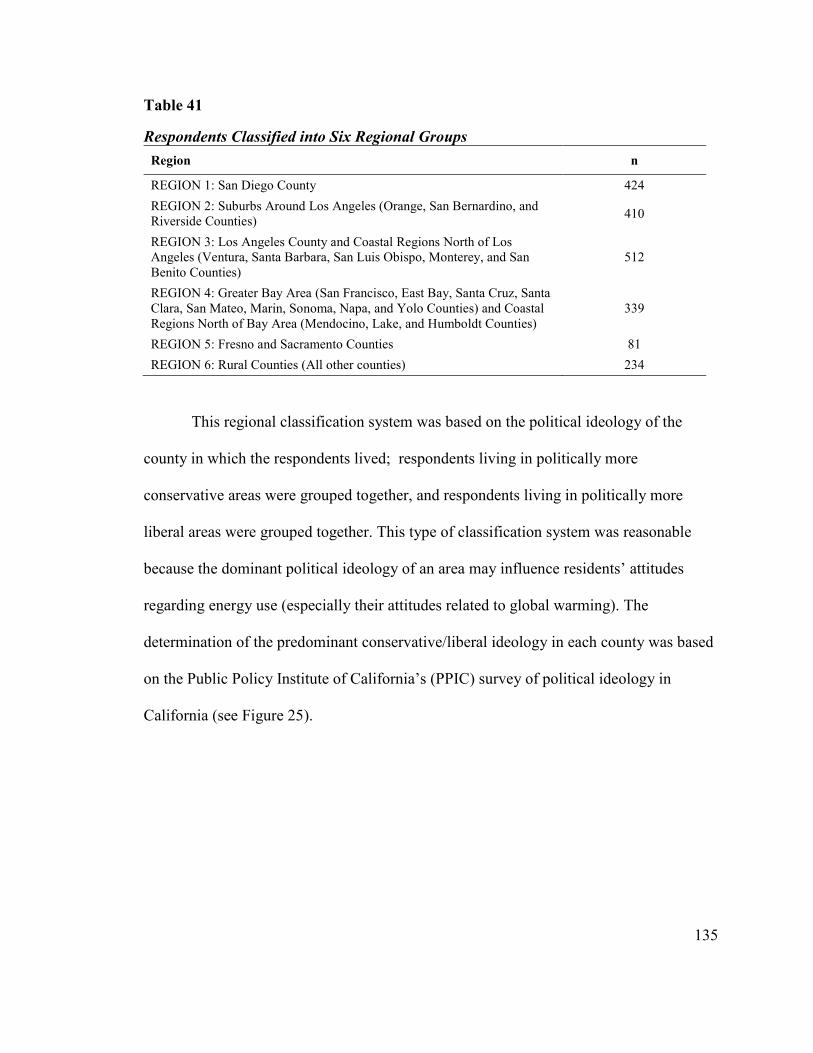
135

Table 41

Respondents Classified into Six Regional Groups

Region n

REGION 1: San Diego County 424

REGION 2: Suburbs Around Los Angeles (Orange, San Bernardino, and Riverside Counties)

410

REGION 3: Los Angeles County and Coastal Regions North of Los Angeles (Ventura, Santa Barbara, San Luis Obispo, Monterey, and San Benito Counties)

512

REGION 4: Greater Bay Area (San Francisco, East Bay, Santa Cruz, Santa Clara, San Mateo, Marin, Sonoma, Napa, and Yolo Counties) and Coastal Regions North of Bay Area (Mendocino, Lake, and Humboldt Counties)

339

REGION 5: Fresno and Sacramento Counties 81

REGION 6: Rural Counties (All other counties) 234

This regional classification system was based on the political ideology of the

county in which the respondents lived; respondents living in politically more

conservative areas were grouped together, and respondents living in politically more

liberal areas were grouped together. This type of classification system was reasonable

because the dominant political ideology of an area may influence residents’ attitudes

regarding energy use (especially their attitudes related to global warming). The

determination of the predominant conservative/liberal ideology in each county was based

on the Public Policy Institute of California’s (PPIC) survey of political ideology in

California (see Figure 25).

136

Figure 25: PPIC Map of Political Ideology in California Across Counties

Note 1: Numbers represent the average response in each county to the question “Would you consider yourself to be politically very liberal, somewhat liberal, middle-of-the-road, somewhat conservative, or very conservative?” Responses were assigned a number: 1.00 (very liberal), 0.50 (liberal), 0 (middle-of-the-road), -0.50 (conservative), -1.00 (very conservative). SOURCE: PPIC Statewide Survey: January, March, May, August, September, October, November 2008; January, February, March, April, May, July, September, November, December 2009; January, March, April, May 2010.


Analysis revealed that those living in rural counties had the lowest number of

CFLs in their homes, on average, while those living in suburbs of Los Angeles had the

137

greatest number of CFLs in their homes, on average (see Table 42). Both of these regions

were more conservative than other regions in California.

Table 42

CFL Installation in Each Region

Region

Political Ideology of

the Region

Mean Number of

CFLs in the Home n

REGION 1: San Diego Middle of the road 9.5 424

REGION 2: Suburbs Around Los Angeles More conservative 10.1 410

REGION 3: Los Angeles and Coastal Regions North of Los Angeles

More liberal 9.5 512

REGION 4: Greater Bay Area More liberal 9.6 339

REGION 5: Fresno and Sacramento Middle of the road 9.3 81

REGION 6: Rural Counties More conservative 8.7 234

7.4.2 CFL Installation Regional OLS Regression Models

The first regional OLS model examined the attitude-behavior relationships while

controlling for demographic and external factors, including the regions referenced above.

In this model, nine variables were significant: the environmental attitude, the global

warming attitude, agreement with the statement “the cost of energy makes me want to

conserve,” income, number of people living at home, whether respondent noted any other

race/ethnicity besides “white” or “Hispanic,” monthly energy expenditures, awareness of

the ENERGY STAR label, and awareness of the carbon footprint concept (see Table 43).

Two variables were marginally significant: agreement with the statement “I sometimes

worry whether there is enough money to pay my energy bill” and house type (see Table

43). The regional variables were not significant. The overall model fit was significant

(F=11.6, p<0.05) and the model explained a small amount of variance (R²=0.11).

138

Table 43

CFL Installation Regional Model 1 Results (2010 CA Data)

Variables Description Std. Coefficients

(n=2000)


.07**


.07**

Economic

Considera-

tions

Household Income (1=less than $20k to 8=more than $80k) .09**


.03**


-.09ᵻ


-.02

House and

Household

Attributes


House Type (1=Single-family Home, 0=Other) .04ᵻ





Region Region (Bay Area=0, San Diego=1, L.A. Suburbs=0, L.A. & Coast North of L.A.=0, Fresno & Sacramento=0, Rural areas=0)

.004

Region (Bay Area=0, San Diego=0, L.A. Suburbs=1, L.A. & Coast North of L.A.=0, Fresno & Sacramento=0, Rural areas=0)

.01


.02


.03


-.001

Energy Price Average monthly bill for all types of energy used in the home, electricity, natural gas, LPG, fuel oil, etc. (Six categories: 1=Less than $50 to 6=More than $250)

.09**



R² .11



Note: Dependent variable is CFL installation behavior. Missing data were imputed (see Section 5.2.2).

139

The next OLS models included the attitude-region interaction terms to assess

whether attitude-behavior relationships were different in areas that were politically liberal

versus middle-of-the-road or conservative. No significant interactions were observed, as

noted in Table 44. This demonstrates that attitude and CFL installation behavior were not

dependent on living in a politically liberal versus middle-of-the-road or conservative area.

140

Table 44

CFL Installation OLS Models with Attitude-Region Interaction Terms (2010 CA Data)

Variables

Standardized Coefficients (n=2000), Models 2-11

2 3 4 5 6 7 8 9 10 11

NOT ALL PARAMETERS SHOWN – These models also included: Env. attitude, global warming attitude, income, two energy cost items, home ownership, house type, # of people living in the home, age, regional variables, average monthly energy bill, and awareness of ENERGY STAR and carbon footprint. Appendix D shows all the parameters. This table presents only std. coefficients of the interaction terms.

Env. Attitude * San Diego (Bay Area is the reference group)

-.10 -- -- -- -- -- -- -- -- --

Global Warming Attitude * San Diego

-- -.01 -- -- -- -- -- -- -- --

Env. Attitude * L.A. Suburbs

-- -- .04 -- -- -- -- -- -- --

Global Warming Attitude * L.A. Suburbs

-- -- -- -.02 -- -- -- -- -- --

Env. Attitude * L.A./North Coast

-- -- -- -- .07 -- -- -- -- --

Global Warming Attitude * L.A./North Coast

-- -- -- -- -- .04 -- -- -- --

Env. Attitude * Fresno/Sacramento

-- -- -- -- -- -- .04

-- -- --

Global Warming Attitude * Fresno/Sacramento

-- -- -- -- -- -- -- -

.001 -- --

Env. Attitude * Rural Areas

-- -- -- -- -- -- -- -- -.03 --

Global Warming Attitude * Rural Areas

-- -- -- -- -- -- -- -- -- .02

R² .11 .11 .11 .11 .11 .11 .11 .11 .11 .11

ANOVA Model Fit

Statistics (F value

and Significance)

11.1,

p<.01

11.0,

p<.01

11.1,

p<.01

11.0,

p<.01

11.1,

p<.01

11.0,

p<.01

11.1,

p<.01

11.0,

p<.01

11.0,

p<.01

11.0,

p<.01




141

8. CONCLUSIONS AND DISCUSSION

8.1 Financial Factors Moderate Attitude-Behavior Relationship

Because the attitude-behavior relationships, in many fields, have often been

influenced by other factors (Stern, 2007; Kraus, 2011), there is considerable interest in

understanding the interdependencies between situational factors, attitudes, and behaviors.

In this study, it was found that the financial constraints (self-reported household income

and average monthly energy expenditures) moderate21 the relationship between the

environmental attitudes and CFL installation behavior (a low-cost energy-saving

behavior). The higher the income or the household energy expenditures, the stronger the

relationship between the pro-environmental attitude and CFL installation (i.e., if you are

more concerned about the environment, then you are more likely to have more CFLs at

home). This pattern was not observed with the thermostat-setting behavior (a non-

purchase behavior). This indicates that household budget (as measured by income and

average monthly energy expenditures) influences the attitude-behavior relationship when

the behavior in question is a low-cost energy-efficient product purchase and not a no-cost

conservation action.

What does this relationship mean? It indicates that attitudes could affect behavior

only in very limited situations. For example, those individuals who hold a pro-

environmental attitude and have larger budgets will buy more CFLs for their home,

21 A variable can be said to moderate the attitude-behavior relationship if the correlation between attitude and behavior varies at different levels of that variable (Baron and Kenny, 1986). This was indicated by the

results of testing various attitude-socio-demographic interaction terms in the regression models.

142

whereas those with lower budgets who hold a similar attitude will not. Thus,

interventions based on psychological factors such as attitudes – information, persuasion,

or social marketing (Stern, 2007) – are likely to make a more significant impact when

targeting either a no-cost behavior or those situations where financial resources are

sufficient to comfortably allow the consumer to participate.

In the last decade, policy makers and program administrators have focused on

providing financial incentives to encourage adoption of energy-efficient lighting

technologies. The aim of these programs, which are typically run by utilities, is to

decrease the cost of energy-efficient bulbs in the marketplace. These programs have

made significant progress in the last decade; energy savings from CFLs have been

enormous and cost-effective (Environmental Protection Agency, 2011). However, this

trend likely will change in the near future as discussed in the next section.

8.2 Remaining Energy Savings Potentials

Two notable findings emerged from this study: (1) among those who had access

to a thermostat, a high percentage (80-90%) reported changing thermostat settings to save

energy, and (2) the percentage of those reporting one or more than one CFL bulb at home

increased from 42% in 2004 to 76% in 2010. Given these findings, it is important to ask

whether there is still some energy savings potential left by pursuing interventions that

target these behaviors.

With respect to CFL installation behavior, the current market is not saturated

with efficient bulbs. Most (three-quarters) light sockets in the U.S. still contain

incandescent light bulbs (Environmental Protection Agency, 2011). This pattern may

143

change in the near future since the new U.S. lighting standard, established by the 2007

Energy Independence and Security Act (EISA), requires that by 2014 a common light

bulb must be at least 25% more efficient than the comparable bulb of 2008. Thus, new

halogen incandescent bulbs, more efficient than the traditional incandescent bulbs, CFLs,

and LEDs will be the only common bulbs manufactured for the U.S. market starting in

2014. This means that many organizations, utilities, or regulators who manage and/or

fund programs that subsidize energy-efficient lighting will face declines in energy

savings that they can claim from their lighting programs, due to a combination of

increased baseline efficiency (due to EISA) and also generally higher naturally occurring

adoption of more-efficient bulbs, especially LEDs (U.S. Department of Energy, 2014).

To phrase it differently, the two factors referenced above contribute to lower program

savings because programs typically cannot claim savings for the efficient bulbs that

would have been purchased regardless of whether the subsidy was available (this is called

“free-ridership” in the energy efficiency industry, and higher free-ridership threatens the

cost-effectiveness of the program). This means that the potential energy savings of

programs that pursue CFL and LED adoption (two easy-to-perform and low-cost

behaviors) are diminishing.

With respect to the thermostat-setting behavior, this study’s findings suggest that

most people are performing this behavior; however, it is not known to what extent. The

survey questions measuring this behavior did not capture enough detail to ascertain to

what extent respondents changed their thermostat setting (e.g., did they lower the setting

from 70⁰F to 68⁰F or 70⁰F to 60⁰F when they were sleeping). Because of this lack of

detail, it was not possible to determine whether more energy savings could be gained by

144

targeting this behavior. Yet, understanding how much more savings, if any, could be

gained by targeting this behavior is an important question to answer because many

utilities are evaluating the energy savings potential of new “smart” thermostats (Peffer et

al., 2011). Smart thermostats have many features and capabilities that older thermostats

lack, such as digital displays, programmable features, or interaction with the wi-fi or

home area network. The Peffer et al. (2011) review revealed that half of the households

with smart thermostats failed to use them as designed, and that the energy savings from

these devices were less than anticipated. It should be acknowledged that it is difficult to

evaluate the energy savings potential of smart thermostats because they are evolving; the

number of new features is increasing and the usability of these devices is improving. The

appeal of smart thermostats as a tool for achieving energy savings is that they can display

various signals (e.g., price, messaging, information), and utilities may control the device

remotely if the occupant approves it. Thus, knowing the potential of energy savings

associated with thermostat-setting behavior (if any) will help determine if it is valuable

for energy efficiency program providers and other stakeholders to target this behavior.

This information could be obtained through a survey that asks respondents to report their

winter daytime and nighttime thermostat settings. Specifically, at what temperature is the

thermostat typically set when respondents are at home and awake, asleep, or when no one

is at home, in the winter? These questions would elicit relevant information to examine to

what extent people change their thermostat settings when they are not at home or are

sleeping – two scenarios of interest in determining whether more energy savings could be

gained by targeting this behavior. If it is learned that there is a significant energy savings

potential from this behavior, then smart thermostats could offer a promising avenue

145

through which to implement various interventions. These interventions could include

messaging about the environment – a motivation for changing a thermostat setting to save

energy. Even if the effect of such an intervention appears to be small, as suggested by this

study, even such a small effect can be substantial when applied to a large population.

This was documented by Opower Home Energy Report experiments, in which residents

received reports of their home’s energy usage and a comparison of their consumption to

their neighbors’ (Allcott, 2011). These experiments achieved energy savings of 2%, on

average; were cost effective for the utilities implementing; and achieved substantial

cumulative kWh savings.

8.3 Attitude-Behavior Relationship Is Weak but Persistent

Although this study confirmed that environmental attitudes were positively and

significantly related to no-cost and low-cost behaviors (thermostat-setting and CFL

installation behavior), this pattern was weak (accounted for less than 10% of behavioral

variance) and was not dependent on time (remained the same regardless of the year in

which the survey was conducted).

It is not uncommon to observe that attitudes explain a small amount of behavioral

variance. Prior attitude-behavior studies demonstrated that attitude-behavior correlations

were rarely above .50, and that attitudes, therefore, rarely accounted for more than 20%

of the behavioral variance (Kraus, 1995). Fazio and Zanna (1981) and Ajzen and

Fishbein (1980) suggested that the attitude-behavior correlation depends on the

measurement match between attitudes and behavior. Fishbein and Ajzen (1977) observed

that attitude-behavior correlations were higher when attitudes correspond to the

146

behavioral measure. For example, a general attitude toward the environment should

predict a general behavior consisting of actions, such as recycling or engaging in energy-

saving behaviors. This research study examined a general environmental attitude and a

more specific behavior (thermostat-setting and CFL installation behavior), which may

explain a low correlation between these behaviors and the environmental attitude. Future

research should expand upon this research and assess whether more specific attitudes

toward thermostat-setting and CFL installation behavior relating to the environment

would better predict those behaviors.

Furthermore, prior studies of household energy behaviors have shown that

attitudes about comfort, conservation, and social norms are related to energy-saving

behaviors (Seligman et al., 1979; Beck, Doctors & Hammond, 1980; Becker et al., 1981;

Brown, 1984; Hand, 1986; Schultz, 1999; Cialdini, 2005; Nolan et al., 2008). However,

none of these studies examined whether attitude-behavior relationships persisted over

time. This study, by examining longitudinal empirical data (where researchers asked the

same questions in each wave of the survey to different samples of people), provides

evidence that the observed pro-environmental attitude-behavior relationship, although

weak, persists over time. The importance of this finding is that it indicates that the size of

the pro-environmental attitudinal effect on energy behavior is likely small and will

continue to be small. This should not invalidate the importance of attitude-behavior

relationships, because other non-attitudinal factors that could explain the behaviors tested

in this study also are weakly related to these behaviors, as discussed in the next section.

147

8.4 Non-attitudinal Variables Also Explain a Small Amount of Variance

Many social scientists point out that factors influencing household energy

efficiency and/or conservation behaviors can vary greatly across behaviors and places

(Lutzenhiser, 1993; Stern, 2007), and that the strongest predictors of these behaviors

often are situational variables, such as weather, availability of the technology, costs, or

regulatory policies (Stern, 2007). This study showed that the situational variables

examined in this study were weak predictors of the behavior, which supports a more

general finding in the social psychology literature that the correlations with situational

determinants of behavior typically are weak to moderate (in the range of .30 to .40)

(Kraus, 1995). The regression models tested in this study included several important

socio-demographic situational variables that can influence energy efficiency and/or

conservation behavior (identified from prior studies): household income, home

ownership, house type, region of residence (Northwest, Midwest, West, or South U.S.),

household size, and age. The models also included several external situational variables

that can influence energy efficiency and/or conservation behaviors: price of heating fuel

(electricity, natural gas, propane, or oil), cumulative number of HDDs in the state of

residence 12 months prior to when the survey was conducted, price of CFLs in the region

of residence, and dollars spent per capita on energy efficiency programs in the state of

residence. When these situational variables were added to the regression models that

included attitudinal and time variables, these variables did not notably increase the

amount of behavioral variance explained; pseudo R2 and R2 values increased from .04 to

.08 and from .10 to .16, respectively.

148

8.5 Encouraging Energy-saving Behavior Requires a Multipronged Intervention

Overall, findings from this study suggest that thermostat-setting and CFL

installation behavior have multi-factorial influences. As noted in the results sections

(Chapters 6 and 7), many different types of variables were significant predictors of these

behaviors: (1) year when the survey was conducted, (2) pro-environmentalal attitude, (3)

socio-demographic variables (e.g., income and household size), (4) awareness of the

ENERGY STAR label or carbon footprint concept, and (5) a few interaction terms

between the pro-environmental attitude and household income/energy expenditures. Prior

research also documented, more broadly, that environmentally significant behaviors,

including energy efficiency and/or conservation behavior, have multi-factorial influences

(Lutzenhiser, 1993; Stern, 2007; Wilson & Dowlatabadi, 2007). For example, general

environmental attitudes can create a general predisposition to act, which may turn into a

specific action that is determined based on personal capabilities (Stern, 2007). Or,

financial incentives can encourage higher-cost behaviors; nevertheless, those will not

occur unless individuals are aware that the incentives are available (Stern, 1999).

Since the behaviors in this study appear to have multi-factorial influences, future

interventions targeting these behaviors should be multi-pronged. Multi-pronged

interventions are those that include more than one type of strategy to affect a behavior

(e.g., using messaging and rebates together). Using multiple strategies will influence a

broader set of underlying influences of the behavior than if only one strategy was used.

Winett et al. (1982) experimental studies showed that multiple strategies, videotape

modeling showing how to save energy and providing daily energy-use feedback, resulted

in overall electricity reductions of about 15%. The feedback and modeling combination

149

was more effective than modeling alone. Further research should explore the effect of

multiple strategies or multi-pronged interventions on the no-cost or low-cost behaviors.

Studying multi-pronged interventions will provide a better sense of the causal

dependencies regarding how attitudes and other factors interrelate and affect behavior.

Various multi-pronged interventions may have a small effect on no-cost or low-

cost energy-saving behaviors. As noted previously, even a small effect is worth pursuing.

For example, if 1% of households in Portland, Oregon (~2,500) converted five 60-watt

incandescent bulbs to 13-watt CFL bulbs today, each household would save enough

energy (~280 kWh per year) to offset 210 pounds of CO2 per year and save $30 per year

on their utility bill.22 Cumulatively, this 1% of households would offset 525,000 pounds

of CO2 and save $75,000 per year.

8.6 Current Energy Policies Appear to Affect the Marketplace

In addition to finding that the amount of money per capita spent on energy

efficiency programs in the state of residence was a marginally significant predictor of

both behaviors in the national samples, it also was found that the awareness of the

ENERGY STAR label was significantly and positively associated with CFL installation

behavior in both the national and California datasets. The federally funded ENERGY

STAR program promotes energy-efficient products in the U.S. marketplace by labeling

them as ENERGY STAR. The level of recognition of this label has been growing in the

U.S. since 2000; about 80% of the population was aware of this label in 2012

22 This was calculated using the calculator from the Environmental Protection Agency

(http://www.epa.gov/climatechange/ghgemissions/ind-calculator.html).

150

(Environmental Protection Agency, 2012). A similar pattern has been found in the survey

data examined in this study; the respondents’ awareness of the ENERGY STAR label

increased from 44% in 2002 to 79% in 2010.

Specifically, the ENERGY STAR program compares various products’ energy

use and cost savings and identifies those products that are more-efficient and cost-

effective over the long term by labeling them ENERGY STAR. To confirm that the self-

reported awareness of the ENERGY STAR label was a good measure of success of the

ENERGY STAR program, additional analysis was performed. Survey respondents who

were aware of the ENERGY STAR label were asked to report its meaning using the

series of statements listed in Table 45. Respondents were asked to indicate whether each

statement described the ENERGY STAR label, or not. The vast majority (more than

80%) of those who were aware of ENERGY STAR reported that the label meant that "the

product uses energy more efficiently than a comparable model" or that “the product, even

if it costs more up front, will save you money over its life.” A smaller percentage of

respondents reported that the label meant "the product is friendly to the environment" or

“the product helps reduce global warming” (see Table 45). These findings indicate that

respondents’ awareness of ENERGY STAR relates to what the ENERGY STAR program

has been doing since its inception – primarily rating and comparing products in terms of

energy and cost savings, and disseminating that information to the public through use of

the ENERGY STAR label. Thus, it can be argued that the awareness of the ENERGY

STAR label is a good measure of the intended outcome of the ENERGY STAR program.

Since awareness of the ENERGY STAR label was a significant predictor in the CFL

151

regression models, this lent support to the assertion that this program is indeed having the

desired effect in the marketplace.

Table 45

Meaning of ENERGY STAR label (Pooled 2002-2010 National Data)

Percentage of those reporting

ENERGY STAR means…by Year

2002

n = 396

2004

n = 438

2006

n = 516

2008

n = 546

2010

n = 321

The product uses energy more efficiently than a comparable model

67% 89% 92% 91% 92%

The product, even if it costs more up front, will save you money over its life

45% 80% 82% 82% 84%

The product is friendly to the environment

31% 72% 76% 74% 72%

The product helps reduce global warming

Not asked Not asked Not asked 62% 57%

The product is of high quality 21% 50% 47% 49% 50%

The government backs this symbol, so you can trust it

19% 36% 35% 43% 47%

Something else 5% 19% 15% 14% 13%

8.7 Concluding Remarks and Policy Implications

This study extended the existing literature in several directions. First, it

documented that the relationship between the pro-environmental attitude and no- and

low-cost energy-saving behavior persisted over time (from 2002 to 2010) in the expected

direction (the association was positive but weak). Prior research on this topic was cross-

sectional, examining only one point in time. This study addresses this gap in literature by

examining attitude-behavior relationships across multiple years.

Second, the findings from this study support the notion that attitudes could affect

behavior in two situations: (1) when targeting either a no-cost behavior, or (2) where

152

financial resources are sufficient to comfortably allow the consumer to participate. This is

important information to know when considering how to design interventions to affect

the two behaviors examined in this study. Nevertheless, this study documented that most

people in the U.S. reported changing thermostat settings to save energy or installing a

CFL (a contribution to the current literature). This finding raises two questions: (1)

whether these two behaviors should be pursued if they are becoming more common in the

population, and (2) at what point in time might the energy savings potential of these two

behaviors no longer be cost-effective to pursue. Further research is needed to answer

these questions. This type of information will help determine whether organizations,

policy makers, and others should pursue these behaviors.

Last, the study showed that thermostat-setting and CFL installation behaviors

have multi-factorial influences. This supports a broader interdisciplinary perspective that

consideration of the influences of energy-saving behaviors should “acknowledge the

expertise of disciplinary approaches but seek to situate this knowledge within the broader

context of energy consumption including social and behavioral factors” (Keirstead, 2005,

p. 3067). If energy-saving behaviors are a function of many different variables, of which

none appear to be the “silver bullet” in explaining the behaviors (as noted in this study),

then policy analysis should explore a broader number of causal pathways and entertain a

wider range of interventions than what is typically used today. Today, most utilities and

organizations that implement energy efficiency programs use financial incentives, price

signals, and information to target behaviors. Recently, there has been a push, especially

in California, to expand the toolbox of interventions (Ignelzi et al., 2013). This is a

153

positive trend and particularly important for the development of policies that should yield

significant energy demand reductions.

154

REFERENCES

Abrahamse, W., Steg, L., Vlek, C. and Rothengatter, T. (2005). A review of intervention Studies aimed at household energy conservation. Journal of Environmental

Psychology, 25, 273-291.

Abt. SRBI and Research Into Action (2002-2010). Energy Conservation,

Efficiency, and Demand Response Study. Fort Myers, FL: Abt. SRBI National Center for Energy Research.

Allcott, H. (2011). Social norms and energy conservation. Journal of Public Economics,

95, 1082-1095.

American Council for an Energy-Efficient Economy (ACEEE) (2002). State Scorecard On Utility and Public Benefits Energy-efficiency Programs: An Update. Retrieved March 10, 2010 from http://aceee.org/publications.

American Council for an Energy-Efficient Economy (ACEEE) (2007). The State Energy Efficiency Scorecard for 2006. Retrieved March 10, 2010 from http://aceee.org/publications.

American Council for an Energy-Efficient Economy (ACEEE) (2009). The 2009 State Energy-efficiency Scorecard. Retrieved March 10, 2010 from http://aceee.org/publications.

American Council for an Energy-Efficient Economy (ACEEE) (2010). The 2010 State Energy-efficiency Scorecard. Retrieved January 10, 2012 from http://aceee.org/publications.

American Council for an Energy-Efficient Economy (ACEEE) (2011). The 2011 State Energy-efficiency Scorecard. Retrieved January 10, 2012 from http://aceee.org/publications.

Ajzen, I. (1991). The Theory of Planned Behavior. Organizational Behavior and Human

Decision Processes, 50, 179-211.

Ajzen, I. and Fishbein, M. (1977). Attitude-behavior relations: A theoretical analysis and review of empirical research. Psychological Bulletin, 84, 888-918.

Ajzen, I. and Fishbein, M. (1980). Understanding attitudes and predicting social

behavior. Englewood Cliffs, NJ: Prentice-Hall.

Bandura A. (1977). Social Learning Theory. Englewood Cliffs, NJ: Prentice-Hall.

Baron, R.M., and Kenny, D.A. (1986). The moderator/mediator variable distinction in social psychological research: Conceptual, strategic, and statistical considerations. Journal of Personality and Social Psychology, 51, 1173-1182.

Beck, P., Doctors, S.I., and Hammond, P.Y. (1980). Individual Energy Conservation

Behaviors. Cambridge, MA: Oelgeschlager, Gunn and Hain.

155

Becker, L.J., Seligman, C., Fazio, R.H. and Darley, J.M. (1981). Relating Attitudes To Residential Energy Use. Environment and Behavior, 13, 590-609.

Berry, L. and Schweitzer, M. (2003). Meta evaluation of National Weatherization

Assistance Program Based on State Studies, 1993–2002. Oak Ridge National Laboratory, Report ORNL/CON-488.Retrieved August 10 from http://weatherization.ornl.gov/pdfs/ORNL_CON-488.pdf.

Boardman, A.E., Greenberg, D.H., Vinning, A.R., and Weimer, D.L. (2006).Cost-Benefit

Analysis (3rded.). New Jersey: Pearson Prentice Hall.

Bolsen, T. and Cook, F.L. (2008). The Polls-Trends, Public Opinion on Energy Policy: 1974-2006. Public Opinion Quarterly, 72, 364-388.

Bonneville Power Administration (2009). Residential Segmentation Research. Prepared By Momentum Market Intelligence. Retrieved September 29, 2010, from http://www.bpa.gov/energy/n/segmentation/BPAResidentialSegmentationResearchMethodology03-10-09.pdf.

Borgida, E. and Campbell, B. (1982). Belief relevance and attitude-behavior consistency: The moderating role of personal experience. Journal of Personality and Social


Black, J.S., Stern, P.C. and Elworth, J.T. (1985). Personal and Contextual Influences on Households Energy Adaptations. Journal of Applied Psychology, 70, 3-21.

Brinberg, D. and Cummings, V. (1983). Purchasing generic prescription drugs: An analysis using two behavioral intention models. Advances in Consumer Research,

11, 229-234.

Brown, M. (1984). Change Mechanisms in the Diffusion of Residential Energy Conservation Practices: An Empirical Study. Technological Forecasting and

Social Change, 25, 123-138.

Cacioppo, J.T. and Petty, R.E. (1979). Effects of message repetition and position on cognitive response, recall and persuasion. Journal of Personality and Social


Cialdini, R.B. (2005). Basic Social Influence is Underestimated. Psychological Inquiry,

16, 158-161.

Davidson, A.R., Yantis, S., Norwood, M., and Montano, D.E. (1985).Amount of information about the attitude object and attitude-behavior consistency. Journal of

Personality and Social Psychology, 49, 1184-1198.

Dubin, J. and McFadden D. (1984). An econometric analysis of residential appliance holdings and consumption. Econometrica, 52, 345-362.

Dubin, J.A., Miedema, A.K., and Chandran, R.V. (1986). Price effects of energy-efficient technologies: a study of residential demand for heating and cooling. Rand Journal

of Economics, 17, 310-325.

156

Eagly, A.H., and Chaiken, S. (1993). The psychology of attitudes. Orlando, FL: Harcourt Brace Jovanovich College Publishers.

Enders, C.K. (2010). Applied Missing Data Analysis. New York: The Guilford Press.

Energy Trust of Oregon (2009).2009 Oregon Residential Awareness and Perception

Study. Prepared by Research Into Action. Retrieved September 29, 2010 from http://energytrust.org/About/policy-and-reports/Reports.aspx.

Espey, J. and Espey, M. (2004). Turning on the lights: A meta-analysis of residential electricity demand elasticities. Journal of Agricultural and Applied Economics, 36, 65-81.

Environmental Protection Agency (2011). Next Generation Lighting Programs: Opportunities to Advance Efficient Lighting for a Cleaner Environment. Retrieved October 9, 2014 from http://www.energystar.gov/ia/partners/manuf_res/downloads.

Environmental Protection Agency (2012). National Awareness of ENERGY STAR for 2012. Retrieved November 11, 2013 from http://library.cee1.org.

Environmental Protection Agency (2014). Inventory of U.S. Greenhouse Gas Emissions and Sinks: 1990-2012. Retrieved June 10, 2014 from www.epa.gov.

Fazio, R.H., and Zanna, M.P. (1981). Direct experience and attitude-behavior consistency. In L. Berkowitz (Ed.) Advances in experimental social psychology (Vol.14, pp.161-202). San Diego, CA: Academic Press.

Festinger, L. (1957). A theory of cognitive dissonance. Evanston, IL: Row, Peterson.

Fishbein, M. and Ajzen, I. (1975). Belief, attitude, intention, and behavior: An

introduction to theory and research. Reading, MA: Addison –Wesley.

Fishbein, M., Middlestadt, S.E., and Chung, J. (1986). Predicting participation and choices among first time voters in U.S. partisan election. In S. Kraus and R. Perloff (Eds.), Mass media and political thoughts: An information processing

approach (pp.65-82). Beverly Hills, CA: Sage.

Frederick, S., Loewenstein, G., and O’Donoghue, T. (2002). Time Discounting and Time Preference: A Critical Review. Journal of Economic Literature, 40, 351-401.

Gardner, G.T. and Stern, C.P. (2008).The Short List: The Most Effective Actions U.S. Households Can Take to Curb Climate Change. Environment 50, 13-24.

Geller, H., and Nadel, S. (1994). Market Transformation Strategies to Promote End-Use Efficiency. Annual Reviews of Energy and the Environment, 19, 301-346.

Gillingham, K., Newell, R. and Palmer, K. (2006).Energy-efficiency Policies: A Retrospective Examination. Annual Review of Environment and Resources, 31, 161-192.

157

Gillingham, K., Newell, R. and Palmer, K. (2009). Energy-efficiency, Economics and

Policy. Resources for the Future, report RFF DP 09-13. Retrieved April 2, 2010 from http://www.rff.org/rff/documents/RFF-DP-09-13.pdf.

Goldman, C., Fuller, M.C., Stuart, E., Peters, J.S., McCrae, M., Albers, N., Lutzenhiser, S. and Spahic, M. (2010). Energy-efficiency Services Sector: Workforce Size and Expectations for Growth. Ernest Orlando Lawrence Berkeley National Laboratory, Report LBNL-3987E.

Guagnano, G.A., Stern, P.C. and Dietz, T. (1995). Influences on Attitude-Behavior Relationships: A Natural Experiment with Curbside Recycling. Environment and

Behavior, 27, 699-718.

Guerin, D.A., Yust, B.L. and Coopet, J.G. (2000). Occupant Predictors of Household Energy Behavior and Consumption Change as Found in Energy Studies Since 1975. Family and Consumer Sciences Research Journal, 29, 48-80.

Hackett, B., Lutzenhiser, L. (1991). Social structures and economic conduct: Interpreting variations in household energy consumption. Sociol. Forum, 6, 449-70.

Hargreaves, D. and Tiggemann, M. (2003). The Effect of “Thin Ideal” Television Commercials on Body Dissatisfaction and Schema Activation During Early Adolescence. Journal of Youth and Adolescence, 32, 367-373.

Hand, C.M. (1989). Energy Attitudes, Beliefs and Behavior: A Specification of Situational and Personal Determinants of Residential Conservation Behavior. UMI Dissertation Information Service. (University Microfilms No.86-24, 245).

Heberlein, T.A., and Warriner, G.K. (1983). The Influence of Price and Attitude on Shifting Residential Electricity Consumption from On- to Off-Peak Periods.

Journal of Economic Psychology, 4, 107-130.

Hirst, E. and White, D. (1985). Indoor Temperature Changes After Retrofit: Inferences Based on Electricity Billing Data for Nonparticipants and Participants in the BPA Residential Weatherization Program. Oak Ridge National Laboratory, ORNL/CON-182 Report.

Hox, J. (2010). Multilevel analysis: Techniques and Applications (2nded.). New York: Routledge.

Hu, L. and Bentler, P.M. (1999). Cutoff criteria for fit indexes in covariance structure analysis: Conventional criteria versus new alternatives. Structural Equation

Modeling: A Multidisciplinary Journal, 6, 1-55.

Ignelzi, P., Peters, J., Randazzo, K., Dethman, L., and Lutzenhiser, L. (2013). Paving the Way for a Richer Mix of Residential Behavior Programs. Retrieved October 1, 2014 from calmac.org.

Itron (2008). California Residential Efficiency Market Share Tracking: Lamps 2007. Prepared for Southern California Edison. Retrieved October 3, 2010 from http://www.cee1.org/eval/lighting_files/CA-2008-12-09.pdf.

158

Jackson, L.A., Hodge, C.N., Gerard, D.A., Ingram, J.M., Ervin, K.S. and Sheppard, L.A. (1996). Cognition, Affect, and Behavior in the Prediction of Group Attitudes. Personality and Social Psychology Bulletin, 22, 306-316.

Kallgren, C.A., and Wood, W. (1986). Access to attitude-relevant information in memory as a determinant of attitude-behavior consistency. Journal of Experimental Social


Katz D. (1960). The Functional Approach to the Study of Attitudes. Public Opinion

Quarterly, 24, 163-204.

Katz, T., and Stotland, E. (1959). A preliminary statement to a theory of attitude structure and change. In S. Koch (Ed.), Psychology: A study of Science (Vol. 3, pp. 423-475). New York: McGraw Hill.

Keirstead, J. (2006). Evaluating the applicability of integrated domestic energy consumption frameworks in the UK. Energy Policy 34, 3065-3077.

KEMA (2010). 2009-2010 Residential Lighting Market Research Study. Prepared for Northwest Energy-efficiency Alliance (NEEA). Retrieved October 3, 2010 from http://neea.org/resource-center/market-research-and-evaluation-reports.

KEMA, the Cadmus Group, Itron, PA Consulting Group, and Jai J. Mitchell Analytics (2010). Final Evaluation Report: Upstream Lighting Program. Prepared for California Public Utilities Commission. Retrieved October 3, 2010 from http://www.energydataweb.com/cpucFiles/18/FinalUpstreamLightingEvaluationReport_2.pdf.

Knussen, K., & Yule, F. (2008). “I’m not in the habit of recycling”: The role of habitual behavior in the disposal of household waste. Environment and Behavior, 40, 683-701.

Kraus, S.J. (1995). Attitudes and Prediction of the Behavior: A Meta Analysis of the Empirical Literature. Personality and Social Psychology Bulletin, 21, 58-75.

Kristom, B. (2008). Residential Energy Demand. In OECD report, Household

Behavior and The Environment: Reviewing the Evidence (Ch.4, pp.95-115). OECD: Paris.

Liska, A.E. (1984). A critical examination of the causal structure of the Fishbein/Ajzen attitude-behavior model. Social Psychology Quarterly, 47, 61-74.

Lutzenhiser, L. (1993). Social and Behavioral Aspects of Energy Use. Annual Review of

Energy and the Environment 18, 247-289.

Lutzenhiser, L. and Gossard, M.H. (2000).Lifestyle, Status and Energy Consumption. In Proceedings of the 2000 ACEEE Summer Study on Energy-efficiency in

Buildings, 8:207-222. Washington, DC: American Council for an Energy-Efficient Economy.

159

Lutzenhiser, L. (2002). An exploratory analysis of residential electricity conservation

survey and billing data. Consultant Report for California Energy Commission. Retrieved September 2, 2010 from www.energy.ca.gov/reports/2002-05-20_400-02-006F.PDF.

Lutzenhiser, L. and Bender, S. (2008). The “Average American” Unmasked: Social Structure and Differences in Household Energy Use and Carbon Emissions. In Proceedings of the 2008 ACEEE Summer Study on Energy-efficiency in

Buildings.7: 191-204. Washington, D.C.: American Council for an Energy Efficient Economy.

Lutzenhiser, L., Cesafsky, L., Chappells, H., Gossard, M., Moezzi, M., Moran, M., Peters, J., Spahic, M., Stern, P., Simmons, E., and Wilhite, H. (2009). Behavioral

Assumptions Underlying California Residential Sector Energy-efficiency

Programs. Report for CIEE and the California Public Utilities Commission. Berkeley: California Institute for Energy-efficiency.

MacCallum, R. C., Browne, M. W., and Sugawara, H. M. (1996). Power analysis and determination of sample size for covariance structure modeling. Psychological

Methods, 1, 130-149.

McConnell, C.R. and Brue, S.L. (2005).Economics (16thed.). New York: McGraw-Hill Companies.

Michman, R. D. (1991). Lifestyle Market Segmentation. New York: Praeger. Millar, M.G., and Tesser, A. (1986). Effects of affective and cognitive focus on the attitude-behavior relation. Journal of Personality and Social Psychology, 51, 270-276.

Newell, F. (1997). The New Rules of Marketing. How to Use One-to-One Relationship

Marketing to be the Leader in Your Industry. New York: McGraw Hill.

Nolan, J.M., Schultz, P.W., Cialdini, R.B., Goldstein, N.J., and Griskevicius, V. (2008). Normative Social Influence is Underdetected. Personality and Social Psychology

Bulletin, 34, 913-922.

O’Neill, B.C. and Chen, B.S. (2002). Demographic Determinants of Household Energy Use in the United States. Population and Development Review, 28, Supplement:

Population Environment Methods of Analysis, 53-88.

Parti, M. and Parti, C. (1980). The Total and Appliance-Specific Conditional Demand for Electricity in the Household Sector. The Bell Journal of Economics, 11, 309-321.

Pavlov, I. (1927). Conditioned reflexes: An investigation of the physiological activity of

the cerebral cortex. Translated and edited by G.V. Anrep. London: Oxford University Press.

Peffer, T., Pritoni, M., Meier, A., Aragon, C., and Perry, D. (2011). How people use thermostats in homes: A review. Building and Environment, 46, 2529-2541.

160

Peters, J.S. (1989). Integrating Psychological and Economic Perspectives on Energy

Consumption: The Determinants of Thermostat Setting Behavior. UMI Dissertation Information Service. Retrieved March 13, 2010 from Dissertation Abstracts International Database.

Petty, R.E. and Cacioppo, J.T. (1986). The Elaboration Likelihood Model of Persuasion. New York: Academic Press.

Pomazal, R.J., and Jaccard, J.J. (1976). An informational approach to altruistic behavior. Journal of Personality and Social Psychology, 33, 317-326.

Poteat V.P. (2007). Peer Group Socialization of Homophobic Attitudes and Behavior During Adolescence. Child Development, 78, 1830-1842.

Poyer, D.A., Henderson, L. and Teotia, A.P.S. (1997). Residential energy consumption across different population groups: comparative analysis for Latino and non-Latino households in USA. Energy Economics, 19, 445-463.

Rajecki, D.W. (1982). Attitudes Themes and Advances. Sunderland, MA: Sinauer Associates, Inc.

Reiss, P.C. and White, M.W. (2008).What changes energy consumption? Prices and public pressures. RAND Journal of Economics, 39, 636-663.

Regan, D.T., and Fazio, R.H. (1977). On the consistency between attitudes and behavior: Look to the method of attitude formation. Journal of Experimental Social


Rosenberg, M.J., and Hovland, C.I. (1960). Cognitive, affective, and behavioral components of attitudes. In C.I. Hovland and M.J. Rosenberg (Eds.), Attitude

organization and change: An analysis of consistency among attitude components (pp.1-14). New Haven, CT: Yale University Press.

Saaid, L. (2013). Americans’ Concerns About Global Warming On the Rise. Gallup News Publication. Retrieved November 2013 from www.gallup.com.

Schultz, P. W. (1999). Changing behavior with normative feedback interventions: A field experiment on curbside recycling. Basic and Applied Social Psychology, 21, 25-36.

Seligman, C., Kriss, M., Darley, J.M., Fazio, R.H., Becker, L. and Pryor, J.B. (1979). Predicting summer energy consumption from homeowners’ attitudes. Journal of

Applied Social Psychology, 9, 70-90.

Shipper, L. Bartlett, S., Hawk, D. and Vine, E. (1989). Linking Life-styles and Energy Use: A Matter of Time. Annual Review of Energy, 14, 273-320.

Simon, H. (1957). A Behavioral Model of Rational Choice. In H. Simon (Ed.), Models of

Man: Rational and Social (pp.99-118). New York: John Wiley.

161

Simon, H. (1987). Rationality in Psychology and Economics. In R. Hogarth and M. Singleton, R.A. and Straits, B.C. (2005). Approaches to Social Research (4th Ed.). New York: Oxford University Press. Reder (Eds.), Rational Choice (pp.25-40). Chicago: University of Chicago Press.

Sinclair, S., Dunn, L., & Lowery, B. (2005). The influence of parental racial attitudes on children's automatic racial prejudice. Journal of Experimental Social Psychology,

41, 283-289.

Skinner B.F. (1938). The Behavior of Organisms: An Experimental Analysis. New York: Appleton-Century.

Socolow, R.H. (Ed.). (1978). Saving Energy in the Home – Princeton’s Experiments at

Twin Rivers. Reports of research conducted by the Center for Environmental Studies, Princeton University. Cambridge, MA: Ballinger Publishing Company.

Sonderegger, R.C. (1978). Movers and Stayers: The Resident's Contribution to Variation Across Houses in Energy Consumption for Space Heating. Energy and Buildings, 1, 313-324.

Snyder, M., and Kendzierski, D. (1982). Acting on one’s attitudes: Procedures for linking attitudes and behavior. Journal of Experimental Social Psychology, 18, 165-183.

Snyder, M., and Swann, W.B., Jr. (1976). When actions reflect attitudes: The politics of impression management. Journal of Personality and Social Psychology, 34, 1034-1042.

Stern, P. C. (1997). Toward a working definition of consumption for environmental research and policy. In P. C. Stern, T. Dietz, V. R. Ruttan, R. H. Socolow, and J. L. Sweeney, eds., Environmentally Significant Consumption: Research

Directions, pp. 12–35. Washington, DC: National Academy Press.

Stern, P. C. (2007). Environmentally significant behavior in the home. In A. Lewis (Ed.), The Cambridge Handbook of Psychology and Economic Behaviour (Ch.15). Cambridge: Cambridge University Press.

Swan, L.G. and Ugursal, V.I. (2009). Modeling of end-use energy consumption in the residential sector: A review of modeling techniques. Renewable and Sustainable

Energy Reviews, 13, 1819-1835.

The Cadmus Group, KEMA, Itron, Nexus Market Research, and A. Goett Consulting (2010). Compact Fluorescent Lamps Market Effects Final Report. Prepared for California Public Utilities Commission. Retrieved October 2, 2010 from http://uc-ciee.org/planning-evaluation/7/327/105/nested.

The NMR Group, KEMA, the Cadmus Group, and Tetra Tech (2010). Massachusetts ENERGY STAR® Lighting Program: 2010 Annual Report. Prepared for Energy-efficiency Advisory Council Consultants, Cape Light Compact, NSTAR, National Grid, Unitil, and Western Massachusetts Electric. Retrieved October 3, 2010 from http://www.ma-eeac.org/docs.

162

Tversky, A. and Kahneman, D. (1981). The Framing of Decisions and the Psychology of Choice. Science, 211, 453-458.

U.S. Congress (1978). National Energy Conservation Act. Washington DC: The Library of Congress.

U.S. Congress (2009). American Recovery and Reinvestment Act. Washington, DC: The Library of Congress.

U.S. Department of Energy, Energy Information Administration (EIA) (1996). Residential Energy Consumption Survey Quality Profile (Ch. 7). Retrieved May 2, 2010, from ftp://ftp.eia.doe.gov/pub/consumption/residential/555961g.pdf.

U.S. Department of Energy, Energy Information Administration (EIA) (2008). Carbon Dioxide Emissions: 1990-2008. Retrieved March16, 2013 from http://www.eia.gov/oiaf/1605/ggrpt/carbon.html.

U.S. Department of Energy, Energy Information Administration (EIA) (2009). Residential Sector Energy Intensities: 1978-2005. Retrieved August 30, 2010 from http://www.eia.doe.gov/emeu/efficiency/recs_tables_list.htm.

U.S. Department of Energy, Energy Information Administration (EIA) (2009). Price of Natural Gas for Residential Customers, Retail Price of Electricity for Residential Customers, and Residential Heating Oil Price. Retrieved October 6th, 2009 from http://www.eia.gov.

U.S. Department of Energy, Energy Information Administration (EIA) (2009). Residential Energy Consumption Survey, Energy Consumption in Homes by End Uses. Retrieved January 10, 2014, from ftp://ftp.eia.doe.gov.

U.S. Department of Energy, Energy Information Administration (EIA) (2012). 2011 Annual Energy Review. Retrieved March 10, 2013 from http://www.eia.gov/totalenergy/data/annual/pdf/aer.pdf.

U.S. Department of Energy (DOE) (2012). Energy Savings Potential of Solid-State Lighting in General Illumination Applications. Report retrieved July 20, 2014 from http://apps1.eere.energy.gov/buildings/publications/pdfs/ssl/ssl_energy-savings-report_jan-2012.pdf.

Van den Putte (1991). 20 years of the theory of reasoned action of Fishbein and Ajzen: A

meta analysis.Unpublished manuscript, University of Amsterdam, the Netherlands.

Wade, S.H. (2003). Price Responsiveness in the AEO2003 NEMS Residential and

Commercial Buildings Sector Models. Energy Information Administration, Retrieved December 3, 2008, from http://www.eia.doe.gov/oiaf/analysispaper/elasticity/.

163

Wilhite, H, Shove, E., Lutzenhiser, L., and Kempton, W. (2000). The Legacy of Twenty Years of Energy Demand Management: we know more about individual behavior but next to nothing about demand. In E. Jochem, D. Bouille, and J. Sathaye (Eds.), Society, Behavior, and Climate Change Mitigation (pp.109-126). Dordrecht/Boston/London: Kluwer Academic Publishers.

Wilson, C. and Dowlatabadi, H. (2007). Models of Decision Making and Residential Energy Use. Annual Review of Environment and Resources 32, 169-203.

Winett, R. A., Hatcher, J.W., Fort, T.R., Leckliter, I.N., Love, S.Q., Riley, A.W., and Fishback, J.F. (1982). The effect of videotape modeling and daily feedback on residential electricity conservation, home temperature and humidity, perceived comfort, and clothing worn: winter and summer. Journal of Applied Behavioral

Analysis, 15, 381-402.

Wood, W. and Neal, D.T. (2009). The habitual consumer. Journal of Consumer


Yates, S.M. and Aronson, E. (1983). A Social Psychological Perspective on Energy Conservation in Residential Buildings. American Psychologist, 38, 435-444.

164

APPENDIX A: Descriptions of Variables

165

Table 46

List of 2002-2010 Survey Variables from the National Datasets Question

Types Exact Wording of the Statements/Questions Measurement

Attitudes -

Cognitive,

Affect, and

Intention

1. I am very concerned about the environment. 2. I look for products that are good for the environment. 3. Saving energy helps the environment. 4. We are using up our energy supplies too fast. 5. There is an energy crisis in our country. 6. I worry that the cost of energy for my home will increase. 7. I sometimes worry whether there is enough money to pay my energy bill. 8. I've already done everything I can to save energy in my home. 9. I’m too busy to be concerned with saving energy in my home.

Ordinal scale: from

1=strongly disagree to 5=strongly

agree

Conservation

and Energy

Efficiency

Behaviors

1. Have you used programmable thermostat to automatically set different temperatures at various times of the day or night to save energy? 2. Have you manually adjusted the thermostat to set different temperatures at various times of the day or night to save energy? 3. How familiar are you with compact fluorescent light bulbs (CFLs)? These are not the regular, tube-shaped fluorescent bulbs, but instead may have a round, spiral, or twisty shape and fit into ordinary light fixtures. Are you very, somewhat or unfamiliar with these bulbs. [If

very or somewhat familiar]Do you have any CFL(s) in your home? If so, how many: _?

Ordinal scale from “very familiar” to

“unfamiliar,” Yes/No/ Don’t

Know, and ratio

measurement (# of bulbs in

the home)

Awareness of

Energy

Efficiency

Labels

1. Are you aware of any programs, brands, or labels to certify appliances, electronic equipment, and related products as energy-efficient? What programs, brands, or labels have you heard of? 2. I’d like to describe a symbol that you may find on products like televisions, home appliances... It’s the word “energy” in script, followed by a star - it’s called the ENERGY STAR symbol. To the best of your knowledge have you ever seen the symbol?

Labels or Yes/No/Don’t

Know

Budget 1. For classification purposes only, which of the following categories best describes your [INPUT YEAR] household income before taxes? Just stop me when I get to the right category.

Categories from 1=≤$20K to 8=≥$80K)

Residence

Attributes

1. Is your residence located in a single-family home, duplex, building with 3 or more units, or mobile/manufactured home? 2. Do you rent or own your residence? 3. Location - zip-code/State recorded


Know

Respondent

Attributes

1. In what year were you born? 2. How many people, including yourself, usually live in your household?

3. Of all the people in your household, how many are under 18 years of age?

Ratio

measurement

166

Table 47

Frequencies of All Attitudinal Variables (2002-2010 National Datasets)

Exact Wording of the

Statements

Ratings (1=Strongly Disagree to 5=Strongly Agree)

Year 1 2 3 4 5 DK/ Ref Not Asked


2002 <1% 5% 7% 52% 35% <1% -

2004 <1% 5% 6% 53% 35% <1% -

2006 <1% 4% 5% 57% 33% <1% -

2008 <1% 2% 3% 26% 20% 1% 49%

2010 1% 1% 2% 20% 13% <1% 64%


2002 <1% 8% 10% 59% 22% <1% -

2004 <1% 7% 8% 58% 25% <1% -

2006 <1% 8% 8% 61% 22% 1% -

2008 <1% 4% 3% 33% 14% <1% 45%

2010 <1% 3% 3% 19% 6% 1% 69%


2002 1% 4% 3% 55% 37% <1% -

2004 <1% 3% 2% 55% 38% 2% -

2006 <1% 2% 2% 57% 38% <1% -

2008 <1% 2% 1% 28% 20% <1% 48%

2010 <1% 1% 1% 16% 11% <1% 71%


2002 3% 16% 10% 48% 17% 5% -

2004 2% 14% 10% 43% 27% 5% -

2006 1% 13% 8% 47% 27% 4% -

2008 1% 7% 3% 23% 13% 1% 52%

2010 1% 4% 2% 17% 7% 2% 68%


2002 4% 18% 10% 45% 20% 4% -

2004 2% 14% 8% 45% 28% 3% -

2006 2% 14% 7% 47% 26% 3% -

2008 1% 4% 2% 26% 19% 1% 48%

2010 <1% 5% 1% 15% 9% 1% 68%


2002 2% 9% 5% 48% 36% 1% -

2004 2% 11% 3% 47% 38% <1% -

2006 <1% 7% 5% 52% 34% <1% -

2008 1% 3% 1% 29% 19% 1% 47%

2010 <1% 3% 1% 19% 13% <1% 63%

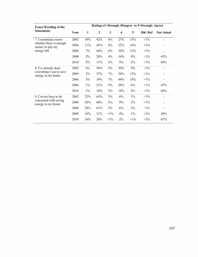
167


Statements

Ratings (1=Strongly Disagree to 5=Strongly Agree)

Year 1 2 3 4 5 DK/ Ref Not Asked


2002 10% 42% 6% 27% 15% <1% -

2004 11% 45% 6% 22% 16% <1% -

2006 7% 44% 6% 30% 13% <1% -

2008 5% 20% 4% 16% 9% <1% 45%

2010 5% 11% 2% 9% 5% <1% 68%


2002 6% 50% 5% 30% 9% <1% -

2004 3% 37% 7% 38% 15% <1% -

2006 3% 34% 7% 44% 10% <1% -

2008 1% 21% 5% 20% 6% <1% 47%

2010 1% 10% 3% 14% 4% <1% 68%


2002 23% 65% 3% 6% 1% <1% -

2004 26% 60% 2% 9% 2% <1% -

2006 28% 61% 3% 6% 2% <1% -

2008 16% 31% <1% 4% 1% <1% 48%

2010 10% 20% <1% 2% <1% <1% 67%

168

Table 48

List of 2010 Survey Variables from the California Dataset Question

Types Exact Wording of the Questions Measurement

Attitudes -

Cognitive,

Affect, and

Intention

1. I am very concerned about the environment. 2. I look for products that are good for the environment. 3. Saving energy helps the environment. 4. Making my home energy-efficient is good for the environment. 5. Global warming is a result of high energy use. 6. People should try to use less energy to reduce global warming. 7. How convinced are you that global warming is happening - would you say not at all, not too convinced, somewhat, mostly, or completely convinced? 8. On a scale of 1 to 5 where 1 is “no impact” and 5 is “a very significant impact,” to what extent do you believe your actions have an impact on the rate or speed of global warming? 9. Saving energy in the home helps me save money. 10. The cost of energy makes me want to conserve. 11. I sometimes worry whether there is enough money to pay my energy bill. 12. I've already done everything I can to save energy in my home. 13. I’m too busy to be concerned with saving energy in my home.

Ordinal scale: from 1=strongly

disagree to 5 or 7=strongly agree or

from 1=not at all convinced/ no

impact to 5=completely

convinced/ a very significant impact

Conservation

and Energy

Efficiency

Behaviors

1. How familiar are you with compact fluorescent light bulbs (CFLs)? These are not the regular, tube-shaped fluorescent bulbs, but instead may have a round, spiral, or twisty shape and fit into ordinary light fixtures. Are you very, somewhat, a little, or not at all familiar with these bulbs? [If very or somewhat familiar] Do you have any CFL(s) in your home? If so, how many: _?

Ordinal scale from “very familiar” to

“not at all,” Yes/No/Don’t

Know, and ratio measurement (# of

bulbs in the home)

Comfort 1. What are some of the obstacles that you currently face in trying to save energy in your home? Desire to maintain comfort, etc.

Labels

Awareness of

Energy

Efficiency

Labels

1. What, if any, programs, brands, or labels have you heard of that indicate that an appliance or piece of electronic equipment is energy-efficient? (unaided awareness of ENERGY STAR) 2. Have you heard of a “carbon footprint”? A “carbon footprint” is a measure of the energy you use throughout your life, either directly or indirectly. This includes, but is not limited to the energy consumption from your home, your transportation, your diet, and your purchases. Have you heard of this now?


Know

Budget 1. For classification purposes only, which of the following categories best describes your [INPUT YEAR] household income before taxes? Just stop me when I get to the right category..

Categories from 1=≤$20K to 8=≥$80K)

Residence

Attributes

1. Is your residence located in a single-family home, duplex, building with 3 or more units, or mobile/manufactured home? 2. Do you rent or own your residence? 3. Location - zip-code indicating region (Bay Area, L.A., etc.)

4. On average, how much is your monthly bill for all types of energy you use in your home, including electricity, natural gas, LPG, fuel oil, and any other fuels? You best estimate is fine. (Six categories: 1=Less than $50 to 6=More than $250)


Know and interval

data

169

Question

Types Exact Wording of the Questions Measurement

Respondent

Attributes

1. In what year were you born? 2. How many people, including yourself, usually live in your household?

3. Of all the people in your household, how many are under 18 years of age?

4. Do you consider yourself: white, Hispanic, African-American, Asian, American Indian, or a member of another race?

Ratio measurement

170

Table 49

Frequencies of All Attitudinal Variables (2010 California Dataset)


Statements

Ratings (1=Strongly Disagree to 5=Strongly Agree, Unless Otherwise

Noted)

1 2 3 4 5 6 7 DK/

Ref

Not

Asked


<1% 1% 1% 9% 5% - - - 84%


<1% 2% 1% 11% 5% - - - 81%


<1% <1% 1% 10% 8% - - <1% 82%

4. Making my home energy-efficient is good for the environment. (7-pt. scale)

28% 4% 2% 2% 2% 1% 3% 1% 57%

5. Global warming is a result of high energy use.

2% 3% 3% 7% 3% - - 1% 82%

6. People should try to use less energy to reduce global warming.

1% 3% 1% 8% 5% - - <1% 82%

7. How convinced are you that global warming is happening - not at all , not too convinced, somewhat, mostly, or completely convinced?

8% 4% 10% 9% 18% - - 1% 51%

8. On a scale of 1 to 5 where 1 is “no impact'”and 5 is “a very significant impact,” to what extent do you believe your actions have an impact on the rate or speed of global warming?

24% 10% 24% 13% 23% - - 6% -

9. Saving energy in the home helps me save money.

0% <1% <1% 9% 8% - - <1% 83%

10. The cost of energy makes me want to conserve.

<1% 1% 1% 10% 8% - - <1% 81%

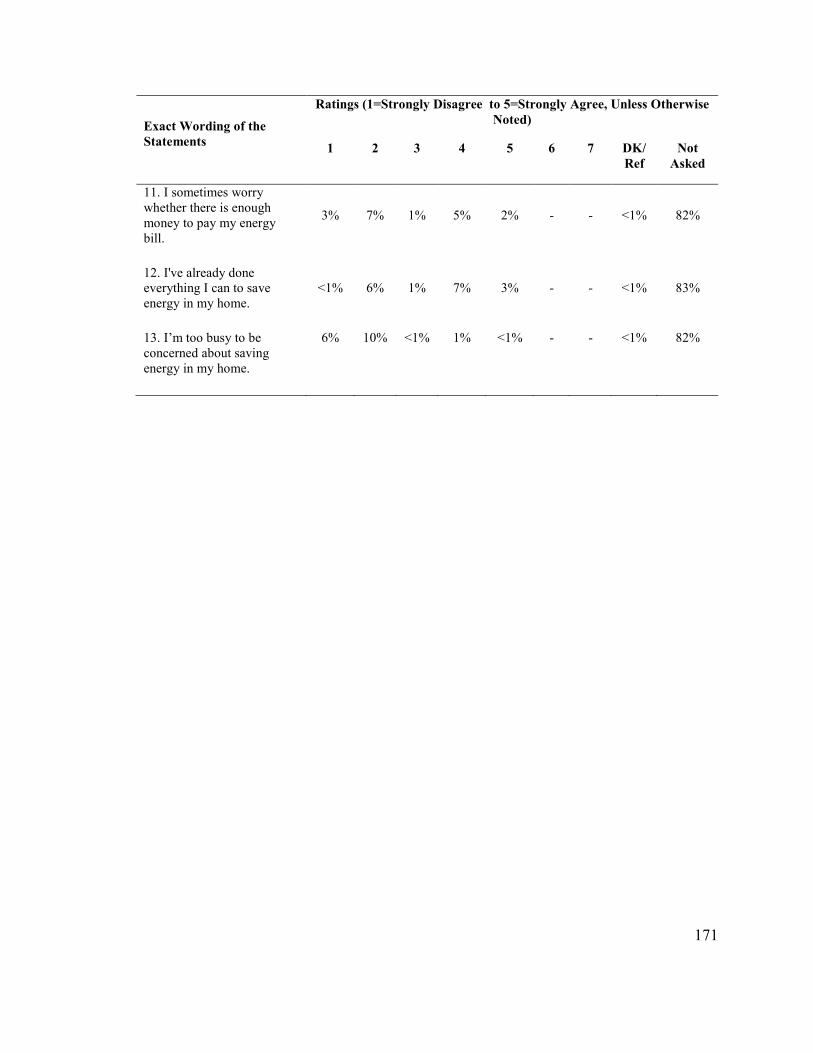
171


Statements

Ratings (1=Strongly Disagree to 5=Strongly Agree, Unless Otherwise

Noted)

1 2 3 4 5 6 7 DK/

Ref

Not

Asked


3% 7% 1% 5% 2% - - <1% 82%


<1% 6% 1% 7% 3% - - <1% 83%

13. I’m too busy to be concerned about saving energy in my home.

6% 10% <1% 1% <1% - - <1% 82%

172

APPENDIX B: Description of the Missing Data Methods

173

Description of the Multiple Imputation Method

There are many statistical approaches to address the problem of missing data. The most sophisticated approaches are Maximum Likelihood and Multiple Imputation techniques (Enders, 2010). This section provides an overview of the Multiple Imputation method, which was used to impute missingdata in this research study.

The Multiple Imputation technique consists of the I-step and the P-step procedures. The I-step procedure uses regression equations to predict missing data values from all other variables that are going to be included in the subsequent analyses (Enders, 2010). The I-step procedure also adds a residual term for each predicted or imputed value to ensure variability of the data are preserved (Enders, 2010). This is known as the stochastic regression imputation.

The P-step procedure uses the imputed data from the I-step to define the distribution of the data and estimate the parameters of that distribution (i.e., the vector mean and the covariance matrix). This is done by using Monte Carlo simulations on the imputed data. These parameter estimates from the Monte Carlo simulations are then used to update the regression coefficients and imputation parameters in the I-step.

Next, the I-step and the P-step procedures are repeated a number of times to generate multiple copies of the data, each having unique estimates of the missing values. The goal is to have multiple datasets containing a random sample of imputations from a distribution of plausible missing values given the observed data.

The IBM SPSS software performs the Multiple Imputation method and generates 20 datasets with imputed values for missing data. These datasets were analyzed to obtain the estimates of the means, correlations, regression coefficients, or any other parameters of interest.

Description of the Maximum Likelihood Method

Another way to handle missing data is to analyze the full but incomplete dataset using Maximum Likelihood estimation. This method, as explained by Enders (2010), uses all the available data to search for the parameters that yield the highest log likelihood or the best fit to the observed data. This method does not fill in the missing values. The log likelihood estimations are computed separately for those cases with complete data on some variables and those with complete data on all variables. Model fit estimation is derived from these two log likelihood estimates. Similar to Multiple Imputation, this method gives unbiased parameter estimates and standard errors.

174

APPENDIX C: Description of CART Analysis

175

Description of CART Analysis

The Classification and Regression Trees (CART) method can identify key characteristics that best predict an outcome variable. This method is analogous to stepwise regression, since it is attempting to determine which predictors explain the most variance among a set of predictors included in the model. Technically, the CART technique produces classification or regression trees. Classification trees are generated when a dependent or outcome variable is categorical. Regression trees are generated when a dependent or outcome variable is continuous.

CART decision trees are generated based on rules and variables included in the analysis. The main rule is to examine all predictors in a model to determine which predictor values would result in the best differentiation of the observations based on the dependent or outcome variable. Once that is determined, the CART algorithm splits cases or observations into groups or nodes to show this differentiation. That is, CART analysis divides the entire sample of households or individuals into subgroups that differ the most in the outcome or dependent variable.

The IBM SPSS software used in this study included the CART algorithm.

176

APPENDIX D: Tables with All Parameters of Select Models

177

Table 50

Thermostat-setting Logistic Regression Models with Socio-Demographic-Attitude

Interactions (Pooled 2002-2006 National Data)

Variables

Odds Ratios (n=1364), Models 9-24

9 10 11 12 13 15 16 17 18 19 21 22 23 24

Env. Attitude - average pro-environmentalal score (lower/higher scores mean lower/higher concern)

2.3 1.5 1.9 1.5 1.2 1.5 3.1 1.5 1.9 1.5 1.4 1.4 1.5 1.5


.91 1.1 .91 1.0 .92 .96 .91 1.5 .92 1.1 .91 .80 .91 .92


1.1 1.1 1.1 1.1 1.1 1.1 1.1 1.1 1.1 1.1 1.1 1.1 1.1 1.1


1.1 1.1 1.1 1.1 1.1 1.1 1.1 1.1 1.1 1.1 1.1 1.1 1.1 1.1


1.0 1.0 1.0 1.0 1.0 1.0 1.0 1.0 1.0 1.0 1.0 1.0 1.0 1.0

Home Ownership (1=Own, 0=Rent) 9.6 3.0 1.2 1.2 1.2 1.2 1.3 1.2 1.2 1.2 1.2 1.2 1.2 1.2

House Type (1=Single-family Home, 0=Other) 1.1 1.1 3.2 1.9 1.1 1.1 1.1 1.1 1.1 1.1 1.1 1.1 .89 1.1

Number of people living in the home 1.3 1.3 1.3 1.3 .89 1.3 1.3 1.3 1.3 1.3 1.3 1.2 1.2 1.3

Age of Respondent (Years) 1.0 1.0 1.0 1.0 1.0 1.0 1.1 1.1 1.02 1.0 1.0 1.0 1.0 1.02

Reside in the Midwest (Northeast=0, Midwest=1, South=0, West=0)

.70 .71 .71 .71 .71 .70 .68 .71 .71 .71 .70 .70 .70 .70


.64 .66 .65 .66 .67 .66 .65 .68 .67 .67 .66 .67 .67 .66


.68 .69 .69 .69 .70 .70 .69 .70 .71 .70 .70 .70 .70 .69

Average Retail Price of Heating Fuel (cents/1000 BTU) in the state of residence

1.1 1.0 1.0 1.0 1.0 1.0 1.0 1.0 1.9 1.5 1.0 1.0 1.0 1.0

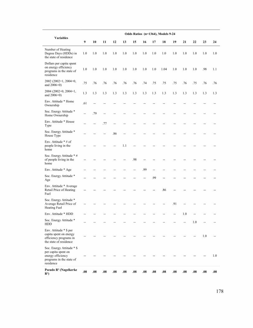
178

Variables


9 10 11 12 13 15 16 17 18 19 21 22 23 24

Number of Heating Degree Days (HDDs) in the state of residence

1.0 1.0 1.0 1.0 1.0 1.0 1.0 1.0 1.0 1.0 1.0 1.0 1.0 1.0


1.0 1.0 1.0 1.0 1.0 1.0 1.0 1.0 1.04 1.0 1.0 1.0 .98 1.1

2002 (2002=1, 2004=0, and 2006=0)

.75 .76 .76 .76 .76 .76 .74 .75 .75 .75 .76 .75 .76 .76

2004 (2002=0, 2004=1, and 2006=0)

1.3 1.3 1.3 1.3 1.3 1.3 1.3 1.3 1.3 1.3 1.3 1.3 1.3 1.3

Env. Attitude * Home Ownership

.61 -- -- -- -- -- -- -- -- -- -- -- -- --

Soc. Energy Attitude * Home Ownership

-- .79 -- -- -- -- -- -- -- -- -- -- -- --

Env. Attitude * House Type

-- -- .77 -- -- -- -- -- -- -- -- -- -- --

Soc. Energy Attitude * House Type

-- -- -- .86 -- -- -- -- -- -- -- -- -- --

Env. Attitude * # of people living in the home

-- -- -- -- 1.1 -- -- -- -- -- -- -- -- --

Soc. Energy Attitude * # of people living in the home

-- -- -- -- -- .98 -- -- -- -- -- -- -- --

Env. Attitude * Age -- -- -- -- -- -- .99 -- -- -- -- -- -- --

Soc. Energy Attitude * Age

-- -- -- -- -- -- -- .99 -- -- -- -- -- --

Env. Attitude * Average Retail Price of Heating Fuel

-- -- -- -- -- -- -- -- .86 -- -- -- -- --

Soc. Energy Attitude * Average Retail Price of Heating Fuel

-- -- -- -- -- -- -- -- -- .91 -- -- -- --

Env. Attitude * HDD -- -- -- -- -- -- -- -- -- -- 1.0 -- -- --

Soc. Energy Attitude * HDD

-- -- -- -- -- -- -- -- -- -- -- 1.0 -- --

Env. Attitude * $ per capita spent on energy efficiency programs in the state of residence

-- -- -- -- -- -- -- -- -- -- -- -- 1.0 --

Soc. Energy Attitude * $ per capita spent on energy efficiency programs in the state of residence

-- -- -- -- -- -- -- -- -- -- -- -- -- 1.0

Pseudo R² (Nagelkerke

R²) .08 .08 .08 .08 .08 .08 .08 .08 .08 .08 .08 .08 .08 .08

179

Variables


9 10 11 12 13 15 16 17 18 19 21 22 23 24

Model Fit Statistics

(Chi-square value and

Significance)

58,

sig

57,

sig

56,

sig

56,

sig

57,

sig

56,

sig

59,

sig

58,

sig

57,

sig

57,

sig

56,

sig

56,

sig

56,

sig

56,

sig

Bold/Highlighted: Significant at p<0.05

Note 1: The dependent variable is thermostat-setting behavior (1=Yes, 0=No). Missing data were excluded from this analysis.

180

Table 51

CFL Regression Models with Socio-Demographic-Attitude Interactions (Pooled 2004-

2010 National Data)

Variables


11 12 13 14 15 16 17 18 19 20 21 22 23 24 25 26


.02 .07 .04 .07 .04 .07 .05 .07 .14 .07 .11 .07 .02 .07 .06 .07


-.02 -.01 -.02 -.01 -.02 .02 -.02 -.01 -.02 -.01 -.02 .02 -.02 -.06 -.02 -.04


.10 .10 .10 .10 .10 .10 .10 .10 .10 .10 .10 .10 .10 .10 .10 .10


-.01

-.01

-.01

-.01

-.01

-.01

-.01

-.01

-.01

-.01

-.01

-.01

-.01

-.01

-.01

-.01


.01 .003 .003 .003 .003 .003 .003 .003 .003 .003 .003 .003 .003 .01 .01 .01

Home Ownership (1=Own, 0=Rent)

-.1 .07 .05 .05 .05 .05 .05 .05 .05 .05 .05 .05 .05 .05 .05 .05

House Type (1=Single-family Home, 0=Other)

.04 .04 -.03 .06 .04 .04 .04 .04 .04 .04 .04 .04 .04 .04 .04 .04

Number of people living in the home

.10 .10 .10 .10 .01 .19 .10 .10 .10 .10 .10 .10 .10 .10 .10 .10

181

Variables


11 12 13 14 15 16 17 18 19 20 21 22 23 24 25 26

Age of Respondent (Years)

.02 .02 .02 .02 .02 .02 .01 .05 .02 .02 .02 .02 .02 .02 .02 .02

Reside in the Midwest (Northeast=0, Midwest=1, South=0, West=0)

.04 .04 .04 .04 .04 .04 .04 .04 .04 .04 .04 .04 .04 .04 .04 .04


.03 .03 .03 .03 .02 .03 .03 .03 .03 .03 .02 .03 .03 .02 .03 .03


.05 .04 .05 .05 .04 .05 .05 .05 .05 .05 .04 .04 .04 .04 .05 .04

Average Retail Price of Electricity (cents/kWh) in the state of residence

.02 .02 .02 .02 .01 .02 .01 .02 .15 .03 .01 .01 .01 .01 .02 .01

Price of CFL bulb in the region of residence ($/CFL)

.01 .01 .01 .01 .01 .01 .01 .01 .01 .01 .08 .06 .01 .01 .01 .01

Number of Heating Degree Days (HDDs) in the state of residence

.03 .02 .02 .02 .02 .02 .02 .02 .03 .02 -.02 .02 -.10 -.1 .02 .02


.05 .05 .05 .05 .05 .05 .05 .05 .05 .05 .05 .05 .05 .05 .03 -.0

Awareness of ENERGY STAR Label (1=Yes, 0=No)

.10 .10 .10 .10 .10 .10 .10 .10 .09 .10 .10 .10 .10 .10 .10 .10

2004 (2004=1, 2006=0, 2008=0, 2010=0)

-.2 -.2 -.24 -.24 -.24 -.24 -.18 -.24 -.24 -.24 -.24 -.24 -.24 -.2 -.2 -.2

2006 (2004=0, 2006=1, 2008=0, 2010=0)

-.2 -.18 -.18 -.18 -.18 -.18 -.24 -.18 -.18 -.18 -.18 -.18 -.18 -.2 -.2 -.2

182

Variables


11 12 13 14 15 16 17 18 19 20 21 22 23 24 25 26

2008 (2004=0, 2006=0, 2008=1, 2010=0)

-.0 -.00 -.00 -.00 -.00 -.00 -.00 -.00 -.00 -.00 -.00 -.00 -.00 -.0 -.0 -.0


.16 -- -- -- -- -- -- -- -- -- -- -- -- -- -- --

Soc. Energy Attitude * Home Ownership

-- -.03 -- -- -- -- -- -- -- -- -- -- -- -- -- --


-- -- .08 -- -- -- -- -- -- -- -- -- -- -- -- --

Soc. Energy Attitude * House Type

-- -- -- -.02 -- -- -- -- -- -- -- -- -- -- -- --


-- -- -- -- .09 -- -- -- -- -- -- -- -- -- -- --

Soc. Energy Attitude * # of people living in the home

-- -- -- -- -- -.10 -- -- -- -- -- -- -- -- -- --

Env. Attitude * Age

-- -- -- -- -- -- .04

-- -- -- -- -- -- -- --

--

Soc. Energy Attitude * Age

-- -- -- -- -- -- -- -.03 -- -- -- -- -- -- -- --

Env. Attitude * Avg. Retail Price of Electricity

-- -- -- -- -- -- -- -- -.16 -- -- -- -- -- -- --

Soc. Energy Attitude * Avg. Retail Price of Electricity

-- -- -- -- -- -- -- -- -- -.03 -- -- -- -- -- --

Env. Attitude * Price of CFL

-- -- -- -- -- -- -- -- -- -- -.08 -- -- -- -- --

Soc. Energy Attitude * Price of CFL

-- -- -- -- -- -- -- -- -- -- -- -.06 -- -- -- --

Env. Attitude * HDD

-- -- -- -- -- -- -- -- -- -- -- -- .13 -- -- --

Soc. Energy Attitude * HDD

-- -- -- -- -- -- -- -- -- -- -- -- -- .08 -- --

Env. Attitude * $/capita spent on energy efficiency programs in the state of residence

-- -- -- -- -- -- -- -- -- -- -- -- -- -- .02 --

183

Variables


11 12 13 14 15 16 17 18 19 20 21 22 23 24 25 26

Soc. Energy Attitude * $/capita spent on energy efficiency programs in the state of residence

-- -- -- -- -- -- -- -- -- -- -- -- -- -- -- .07

R-square .16 .16 .16 .16 .16 .16 .16 .16 .16 .16 .16 .16 .16 .16 .16 .16

ANOVA

Model Fit

Statistics (F

value and

Significance)

28,

sig

28,

sig

28,

sig

28,

sig

28,

sig

28,

sig

28,

sig

28,

sig

28,

sig

28,

sig

28,

sig

28,

sig

28,

sig

28,

sig

28,

sig

28,

sig


Note 1: The ependent variable is CFL installation behavior.


184

Table 52

CFL Installation OLS Models with Socio-Demographic-Attitude Interactions (2010 CA

Data)

Description


4 5 6 7 8 9 10 11 12 13 14 15 16 17


.03 .07 .04 .07 .09 .07 .04 .07 .07 .07 .08 .07 -.02 .07


.07 .01 .07 .04 .07 .09 .07 .04 .07 .07 .07 .07 .07 -.04


.09 .09 .09 .09 .09 .09 .09 .09 .09 .09 .09 .09 .09 .09


.03 .03 .03 .03 .03 .03 .03 .03 .03 .03 .03 .03 .03 .03


-.1 -.09 -.09 -.09 -.09 -.09 -.09 -.1 -.09 -.09 -.09 -.09 -.09 -.09

Those who said desire for comfort is a barrier to saving energy at home (1= Said it, 0=Didn’t say it)

-.0 -.02 -.02 -.02 -.02 -.02 -.02 -.0 -.02 -.02 -.02 -.02 -.03 -.03

Home Ownership (1=Own, 0=Rent) -.1 -.08 .02 .02 .02 .02 .02 .02 .02 .02 .02 .02 .02 .02

House Type (1=Single-family Home, 0=Other) .04 .04 -.06 -.01 .04 .04 .04 .04 .04 .04 .04 .04 .04 .04

Number of people living in the home .06 .06 .06 .06 .13 .11 .06 .06 .06 .06 .06 .06 .06 .06

Age of Respondent (Years) -.0 -.02 -.02 -.02 -.02 -.02 -.07 -.1 -.02 -.02 -.02 -.02 -.02 -.02

Race (White=0, Hispanic=1, Other=0) -.1 -.04 -.05 -.05 -.05 -.04 -.05 -.1 .01 -.01 -.05 -.05 -.04 -.04

Race (White=0, Hispanic=0, Other=1) -.1 -.04 -.04 -.04 -.04 -.04 -.04 -.1 -.04 -.04 .03 -.01 -.05 -.05

Northern/Southern CA (Northern=0, Southern=1) Dividing line is the boundary between Monterey and San Luis Obispo

-.0 -.01 -.01 -.01 -.01 -.01 -.01 -.0 -.01 -.01 -.01 -.01 -.01 -.01

185

Description


4 5 6 7 8 9 10 11 12 13 14 15 16 17

On average, how much is your monthly bill for all types of energy you use in your home, including electricity, natural gas, LPG, fuel oil, and any other fuels? Your best estimate is fine. (Six categories: 1=Less than $50 to 6=More than $250)

.09 .09 .09 .09 .09 .09 .09 .09 .09 .09 .09 .09 -.15 -.08


.07 .07 .07 .07 .07 .07 .07 .07 .07 .07 .07 .07 .07 .07

Awareness of Carbon Footprint Concept (1=Yes, 0=No)

.07 .07 .07 .07 .07 .07 .07 .07 .07 .07 .07 .07 .07 .07


.15 -- -- -- -- -- -- -- -- -- -- -- -- --

Global Warming Attitude * Home Ownership

-- .12 -- -- -- -- -- -- -- -- -- -- -- --


-- -- .11 -- -- -- -- -- -- -- -- -- -- --

Global Warming Attitude * House Type

-- -- -- .05 -- -- -- -- -- -- -- -- -- --


-- -- -- -- -.08 -- -- -- -- -- -- -- -- --

Global Warming Attitude * # of people living in the home

-- -- -- -- -- -.06 -- -- -- -- -- -- -- --

Env. Attitude * Age -- -- -- -- -- -- .06 -- -- -- -- -- -- --

Global Warming Attitude * Age

-- -- -- -- -- -- -- .04 -- -- -- -- -- --

Env. Attitude * Race (Hispanic)

-- -- -- -- -- -- -- -- -.06 -- -- -- -- --

Global Warming Attitude * Race (Hispanic)

-- -- -- -- -- -- -- -- -- -.04 -- -- -- --

Env. Attitude * Race (Other)

-- -- -- -- -- -- -- -- -- -- -.08 -- -- --

Global Warming Attitude * Race (Other)

-- -- -- -- -- -- -- -- -- -- -- -.04 -- --

Env. Attitude* Avg. Monthly Energy Bill

-- -- -- -- -- -- -- -- -- -- -- -- .26 --

Global Warming Attitude * Avg. Monthly Energy Bill

-- -- -- -- -- -- -- -- -- -- -- -- -- .20

R-square .10 .10 .10 .10 .10 .10 .10 .10 .10 .10 .10 .10 .10 .11

186

Description


4 5 6 7 8 9 10 11 12 13 14 15 16 17

ANOVA Model Fit

Statistics (F value and

Significance)

14,

sig

14,

sig

14,

sig

14,

sig

14,

sig

14,

sig

14,

sig

14,

sig

14,

sig

14,

sig

14,

sig

14,

sig

14,

sig

14,

sig





187

Table 53

CFL Installation OLS Models with Attitude-Region Interaction Terms (2010 CA Data) Standardized Coefficients (n=2000), Models 2-11

Variables 2 3 4 5 6 7 8 9 10 11


.08** .07** .06** .07** .06** .07** .06** .07** .07** .07**


.07** .07** .07** .07** .07** .06ᵻ .07** .07** .07** .06**


.09** .09** .09** .09** .09** .09** .09** .09** .09** .09**


-.08** -.08** -.08** -.08** -.08** -.08** -.08** -.08** -.08** -.08**


.03ᵻ .03ᵻ .03ᵻ .03ᵻ .03 .03 .03ᵻ .03ᵻ .03ᵻ .03

Those who said desire for comfort is a barrier to saving energy at home (1= Said it, 0=Didn’t say it)

-.02 -.02 -.02 -.02 -.02 -.02 -.02 -.02 -.02 -.02

Home Ownership (1=Own, 0=Rent)

.02 .02 .02 .02 .02 .02 .02 .02 .02 .02

House Type (1=Single-family Home, 0=Other)

.04ᵻ .04ᵻ .04ᵻ .04ᵻ .04ᵻ .04ᵻ .04ᵻ .04ᵻ .04ᵻ .04ᵻ

Number of people living in the home

.06** .06** .06** .06** .06** .06** .06** .06** .06** .06**

Age of Respondent (Years) -.02 -.02 -.02 -.02 -.02 -.02 -.02 -.02 -.02 -.02

Race (White=0, Hispanic=1, Other=0)

-.04 -.04 -.04 -.04 -.04 -.04 -.04 -.04 -.04 -.04

Race (White=0, Hispanic=0, Other=1)

-.04** -.04** -.04** -.04** -.04** -.04** -.04** -.04** -.04** -.04**

Region (San Diego=1) (Bay Area is the reference group)

.11 .01 .004 .004 .003 .003 .004 .004 .004 .004

Region (L.A. Suburbs=1) .01 .01 -.04 .03 .01 .01 .01 .01 .01 .01

Region (L.A. & Coast North of L.A.=1)

.02 .02 .02 .02 -.05 -.02 .02 .02 .02 .02

Region (Fresno & Sacramento=1)

.03 .03 .03 .03 .03 .03 -.01 .03 .03 .03

Region (Rural areas=1) -.000 -.001 -.001 -.000 -.001 -.001 -.001 -.001 .03 -.02

On average, how much is your monthly bill for all types of energy you use in your home.

.09** .09** .09** .09** .09** .09** .09** .09** .09** .09**

188

(Six categories: 1=Less than $50 to 6=More than $250)


.07** .07** .07** .07** .07** .07** .07** .07** .07** .07**

Awareness of Carbon Footprint Concept (1=Yes, 0=No)

.07** .07** .07** .07** .07** .07** .07** .07** .07** .07**

Env. Attitude * San Diego (Bay Area is the reference group)

-.10 -- -- -- -- -- -- -- -- --

Global Warming Attitude * San Diego

-- -.01 -- -- -- -- -- -- -- --

Env. Attitude * L.A. Suburbs -- -- .04 -- -- -- -- -- -- --

Global Warming Attitude * L.A. Suburbs

-- -- -- -.02 -- -- -- -- -- --

Env. Attitude * L.A./North Coast

-- -- -- -- .07 -- -- -- -- --

Global Warming Attitude * L.A./North Coast

-- -- -- -- -- .04 -- -- -- --

Env. Attitude * Fresno/Sacramento

-- -- -- -- -- -- .04 -- -- --

Global Warming Attitude * Fresno/Sacramento

-- -- -- -- -- -- -- -.001 -- --

Env. Attitude * Rural area -- -- -- -- -- -- -- -- -.03 --

Global Warming Attitude * Rural area

-- -- -- -- -- -- -- -- -- .02

R-square .11 .11 .11 .11 .11 .11 .11 .11 .11 .11

ANOVA Model Fit Statistics

(F value and Significance) 11.1,

p<.01 11.0,

p<.01 11.1,

p<.01 11.0,

p<.01 11.1,

p<.01 11.0,

p<.01 11.1,

p<.01 11.0,

p<.01 11.0,

p<.01 11.0,

p<.01





189

APPENDIX E: Additional CFL Models

190

Table 54

CFL Installation OLS Model 8a Results (Pooled 2004-2010 National Data, Only Those

Who Adopted CFLs)


Std. Coefficients

Model 8a

(n=2022)


.04**


-.02

Economic

Consider-

ations



-.01


.01

House and

Household

Attributes


House Type (1=Single-family Home, 0=Other) .04ᵻ


Age of Respondent (Years) .002




Energy

and

Product

Prices




Energy

Efficiency

Funding


.03


Time 2004 (2004=1, 2006=0, 2008=0, 2010=0) -.18**

2006 (2004=0, 2006=1, 2008=0, 2010=0) -.15**

2008 (2004=0, 2006=0, 2008=1, 2010=0) -.02

R-square .11



191


This excluded cases with zero CFLs in the home.



192

Table 55

CFL Installation OLS Model 8b Results (Pooled 2004-2010 National Data, Only Those

Who Adopted CFLs)


Std. Coefficients

Model 8b

(n=2022)


.05**


-.02

Economic

Considerat

ions



.01


.003

House and

Household

Attributes


House Type (1=Single-family Home, 0=Other) .03






Energy

and

Product

Prices


Price of CFL bulb in the region of residence ($/CFL) -.01


Energy

Efficiency

Funding


.03


Time 2004 (2004=1, 2006=0, 2008=0, 2010=0) -.23**

2006 (2004=0, 2006=1, 2008=0, 2010=0) -.22**

2008 (2004=0, 2006=0, 2008=1, 2010=0) -.04

R-square .17



Note 1: Dependent variable is log transformed – ln(number of CFL bulbs in the home). Excluded those

who had zero CFLs in the home.

193



194

Table 56

CFL Installation OLS Model 1a Results (2010 CA Data, Only Those Who Adopted

CFLs)


Std. Coefficients

Model 1a

(n=1462)


.06


.04

Economic

Considerations


.11**


.03

I sometimes worry whether there is enough money to pay my energy bill (same 5-pt scale) -.09ᵻ


-.02

House and

Household

Attributes






Race (White=0, Hispanic=0, Other=1) -.05ᵻ

Region Northern/Southern CA (Northern=0, Southern=1) Dividing line is the boundary between Monterey and San Luis Obispo

.003


.09**

Knowledge Awareness of ENERGY STAR Label (1=Yes, 0=No) .04

Awareness of Carbon Footprint Concept (1=Yes, 0=No) .04

R-square .10




Excluded those who had zero CFLs in the home.



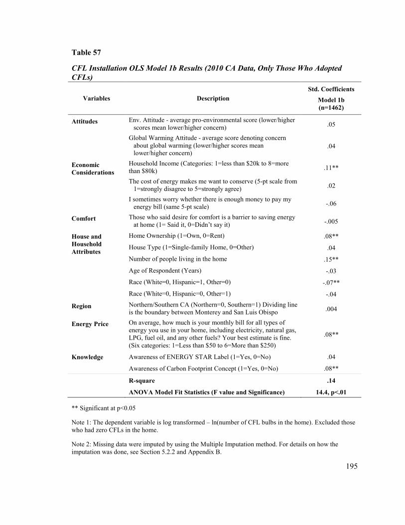
195

Table 57

CFL Installation OLS Model 1b Results (2010 CA Data, Only Those Who Adopted

CFLs)


Std. Coefficients

Model 1b

(n=1462)


.05


.04

Economic

Considerations


.11**


.02


-.06


-.005

House and

Household

Attributes







Region Northern/Southern CA (Northern=0, Southern=1) Dividing line is the boundary between Monterey and San Luis Obispo

.004


.08**

Knowledge Awareness of ENERGY STAR Label (1=Yes, 0=No) .04


R-square .14



Note 1: The dependent variable is log transformed – ln(number of CFL bulbs in the home). Excluded those who had zero CFLs in the home.


196

APPENDIX F: Additional Measurement Limitations

197

Measurement Limitations

Appropriate measurement is crucial for any research inquiry. The main measurement limitations applicable to this research study are noted in this section.

First, self-reported data are the primary source of information for this study. There are two concerns for using self-reported data. The first concern relates to social desirability bias, which is a tendency of the individuals to respond in a manner perceived favorably by others (Singleton and Straits, 2005). It is possible that individuals may give socially desirable answers about their views on conservation. The second concern is that the profile of those choosing not to participate in a survey may be profoundly different from that of the individuals who choose to participate. The cooperation rates for the Energy Conservation, Efficiency, and Demand Response surveys since 2004 were high (see Section 5.1), which minimized this effect. However, it is important to recognize that respondents still might be different from those who refused to participate in the research or from those who were not-reached during the data-collection process.

Second, the human mind has at least two modes of operation: the conscious mode, such as choosing to have an energy audit, and the less-conscious or automatic mode, which can include habitually leaving lights on after leaving a room or space. In the realm of household energy consumption, Lutzenhiser et al. (2010) and Stern (2007) recognized that, besides conscious behaviors, various energy consumption choices are habitual. In thinking about habits, Wood and Neal (2009) described these behaviors as being acquired through life, often cued by context (e.g. place, situation), and “not immune to deliberative processes” (p. 579). Hence, it is feasible that individuals may not be conscious of all the tendencies they act upon when they use energy inside the home. In terms of measurement, this is a challenge since self-reported accounts of attitudes and behaviors from those who volunteered such information may not capture information that is not salient in the individual’s mind. In this study, only attitudes representative of conscious/salient thoughts about the behavior were explored; unconscious tendencies that individuals may have had were not investigated.

Last, one of the main challenges of this study was that a large percentage of survey respondents reported performing thermostat setback and CFL installation behaviors. For example, as many as 90% of survey respondents who had access to a thermostat reported that they changed their thermostat setting to save energy. This lack of variability in the outcome variable was difficult to analyze both methodologically and conceptually, as such a large percentage of respondents reported already participating in the behavior. Still, this concern is not unique to this method of analysis; it is common across many methods used to assess determinants of behavior.

Documents

Energy Efficiency and Conservation Attitudes: An