Energy-Constrained Distinguishability Measures for

Louisiana State University Louisiana State University

LSU Digital Commons LSU Digital Commons

LSU Doctoral Dissertations Graduate School

3-23-2021

Energy-Constrained Distinguishability Measures for Assessing Energy-Constrained Distinguishability Measures for Assessing

Performance in Quantum Information Processing Performance in Quantum Information Processing

Kunal Sharma Louisiana State University at Baton Rouge

Follow this and additional works at: https://digitalcommons.lsu.edu/gradschool_dissertations

Part of the Quantum Physics Commons

Recommended Citation Recommended Citation Sharma, Kunal, "Energy-Constrained Distinguishability Measures for Assessing Performance in Quantum Information Processing" (2021). LSU Doctoral Dissertations. 5495. https://digitalcommons.lsu.edu/gradschool_dissertations/5495

This Dissertation is brought to you for free and open access by the Graduate School at LSU Digital Commons. It has been accepted for inclusion in LSU Doctoral Dissertations by an authorized graduate school editor of LSU Digital Commons. For more information, please [email protected].

https://digitalcommons.lsu.edu/

https://digitalcommons.lsu.edu/gradschool_dissertations

https://digitalcommons.lsu.edu/gradschool

https://digitalcommons.lsu.edu/gradschool_dissertations?utm_source=digitalcommons.lsu.edu%2Fgradschool_dissertations%2F5495&utm_medium=PDF&utm_campaign=PDFCoverPages

http://network.bepress.com/hgg/discipline/206?utm_source=digitalcommons.lsu.edu%2Fgradschool_dissertations%2F5495&utm_medium=PDF&utm_campaign=PDFCoverPages

https://digitalcommons.lsu.edu/gradschool_dissertations/5495?utm_source=digitalcommons.lsu.edu%2Fgradschool_dissertations%2F5495&utm_medium=PDF&utm_campaign=PDFCoverPages

mailto:[email protected]

ENERGY-CONSTRAINED DISTINGUISHABILITY

MEASURES FOR ASSESSING PERFORMANCE IN

QUANTUM INFORMATION PROCESSING

A Dissertation

Submitted to the Graduate Faculty of the

Louisiana State University and

Agricultural and Mechanical College

in partial fulfillment of the

requirements for the degree of

Doctor of Philosophy

in

The Department of Physics and Astronomy

by

Kunal Sharma

BS-MS, Indian Institute of Science Education and Research Bhopal, 2016

May 2021

To my parents

Vishnu and Yogita Sharma

ii

ACKNOWLEDGMENTS

The completion of this dissertation could not have been possible without the help and

support of countless people.

First and foremost, I thank my Ph.D. supervisor Mark M. Wilde for his support,

guidance, and friendship over the last five years. I am grateful to him for devoting many

hours to discussions and explanations on several research topics. His broad expertise in

quantum information science has immensely helped me learn various research topics during

my Ph.D. His perseverance and passion for solving research problems have always inspired

me and many others. I am thankful to him for regularly providing constructive feedback,

which has helped me grow as a researcher. I will always be indebted to him for his constant

support as an advisor and a friend and the opportunities he provided me in the past five

years.

I am grateful to the late Jonathan P. Dowling for showing a lot of confidence in me.

His ability to connect with students and motivate them irrespective of their background is

something I would like to replicate in my life.

I had the privilege to work at the Los Alamos National Lab as a long-term graduate

research assistant during my Ph.D. Many thanks to Patrick J. Coles for providing me with

such an exciting opportunity and for his support and friendship. I am grateful to him for

offering me to lead several research projects and for providing constant feedback. He has

also taught me how to conduct research collaboratively by valuing my opinion in every

research discussion. I am also thankful to Lukasz Cincio for his support and for teaching

me how to be an efficient researcher. I have significantly benefited from his advice on many

academic and non-academic challenges.

I am incredibly grateful to Marco Cerezo and Zoë Holmes for always being available

whenever I needed them. Discussions on research and random topics with them have made

the last two years of my Ph.D. a delightful experience. I could not have asked for better

friends and colleagues. Along with them, many thanks to Piotr Czarnik, Gopikrishnan

iii

Muraleedharan, and Burak Şahinoğlu for making my stay in Los Alamos exciting. Special

thanks to Samson Wang for discussing science and philosophy from the UK.

I thank Barry C. Sanders for his help and for hosting me at the University of Calgary.

Several research discussions with him have helped me develop research ideas and com-

municate them better. I also thank Kamil Bradler, Daiqin Su, Haoyu Qi, and Christian

Weedbrook for their hospitality and many discussions at Xanadu.

I am thankful to several mentors for guiding me over many years. Many thanks to

Pankaj Baluja, Lalit K. Banga, Aditi Sen De, Suvankar Dutta, Suresh Dwivedi, Vibhuti

Dwivedi, Madhu Gupta, Ambar Jain, Ravi P. Rau, Jeyaraman Sankar, Ruchika Sankar,

and Ujjwal Sen. I especially acknowledge Prasun Dutta for asking me fundamental physics

questions a countless number of times and for teaching me the joy of living a simple life. A

special thanks to Michael Nielsen for writing remarkable essays on “principles of effective

research” and “six rules for rewriting,” which have helped improve my scientific approach

immensely over the past few years.

I thank Ivan Agullo, Li Chen, Ravi P. Rau, and Mark M. Wilde for taking out time

to be on my Ph.D. committee and for providing feedback on my work. I am grateful

to Mark M. Wilde for his valuable comments on this thesis. Many thanks to Claire R.

Bullock, Carol Duran, Arnell Nelson, Paige Whittington, Yao Zeng, and other members of

the Department of Physics and Astronomy at LSU for their help during my Ph.D.

I collaborated with many colleagues over the last five years. Many thanks to Sushovit

Adhikari, Andrew Arrasmith, Kamil Bradler, Marco Cerezo, Lukasz Cincio, Patrick J.

Coles, Ish Dhand, Enrico Fontana, Zoë Holmes, Robert Israel, Eneet Kaur, Sumeet Khatri,

Meenu Kumari, Ludovico Lami, Felix Leditzky, Jarrod McClean, Kyungjoo Noh, Haoyu

Qi, Barry C. Sanders, Akira Sone, Andrew Sornborger, Daiqin Su, Yuan Su, Masahiro

Takeoka, Eyuri Wakakuwa, Samson Wang, Xin Wang, Mark M. Wilde, and Yadong Wu.

It has been a pleasure to collaborate with these great researchers.

I have been fortunate to have wonderful friends all around the world. I thank Ja-

iv

cob Beckey, Anthony Brady, Ritwika Chakraborty, Arghya Chattopadhyay, Anirban N.

Chowdhury, Siddhartha Das, Sarah Davis, Arundhati Deshmukh, Himadri S. Dhar, Arpit

Dua, Enrico Fontana, Isabella Goetting, Girraj Goyal, Pinky Goyal, Wendy K. Hahn, Stav

Haldar, Yoshita Holamoge, Samreen Iram, Kevin V. Jacob, Namitha A. James, Geo Jose,

Vishal Joshi, Salini Karuvade, Vishal Katariya, Eneet Kaur, Prateek Khandelwal, Sumeet

Khatri, Meenu Kumari, Dan W. McCarn, Aby Philip, Prateek Raj, Sayonee Ray, Meghan

Ryan, Vinay Sagar, Sahil Saini, Ruchika Shankar, Karunya Shirali, Aliza Siddiqui, Ut-

tam Singh, Alejandra C. Spillari, Sudhanshu Srivastava, Simran Thapa, Justin Yirka, and

Chenglong You. I am grateful to Noah Davis, Siddharth Soni, and Haoyu Qi for their great

friendship and for supporting me throughout my Ph.D. Special thanks to Divya Rastogi

Joshi for the care she put into making me feel at home during the past three years.

Finally, I would like to thank everyone in my family, especially my sister Kanika Sharma

and my parents Vishnu P. Sharma and Yogita Sharma. I am indebted to them for every-

thing they have done for me. I would have never completed this thesis without their love,

care, and encouragement. I am grateful to them for continually supporting my studies and

everything else I do in my life.

v

TABLE OF CONTENTS

ACKNOWLEDGMENTS . . . . . . . . . . . . . . . . . . . . . . . . . . . . . . . . . . . . . . . . . . . . . . . . . . . . . . . . . iii

ABSTRACT. . . . . . . . . . . . . . . . . . . . . . . . . . . . . . . . . . . . . . . . . . . . . . . . . . . . . . . . . . . . . . . . . . . . . . . viii

CHAPTER

1 INTRODUCTION . . . . . . . . . . . . . . . . . . . . . . . . . . . . . . . . . . . . . . . . . . . . . . . . . . . . . . . . . 1

2 PRELIMINARIES . . . . . . . . . . . . . . . . . . . . . . . . . . . . . . . . . . . . . . . . . . . . . . . . . . . . . . . . . 13

2.1 Quantum States and Operations . . . . . . . . . . . . . . . . . . . . . . . . . . . . . . . . . . . . . . 13

2.2 Quantum Entropies and Information . . . . . . . . . . . . . . . . . . . . . . . . . . . . . . . . . . 21

2.3 Bosonic Quantum States and Channels . . . . . . . . . . . . . . . . . . . . . . . . . . . . . . . . 23

2.4 Distance Measures for Quantum States and Channels . . . . . . . . . . . . . . . . . . 42

2.5 Notions of Convergence for Quantum Channels . . . . . . . . . . . . . . . . . . . . . . . . 47

2.6 Approximate Degradability of Quantum Channels . . . . . . . . . . . . . . . . . . . . . 49

2.7 Quantum Channel Capacities . . . . . . . . . . . . . . . . . . . . . . . . . . . . . . . . . . . . . . . . . 50

2.8 Continuity of Information Quantities and Channel Capacities . . . . . . . . . . 53

2.9 Karush-Kuhn-Tucker (KKT) Conditions . . . . . . . . . . . . . . . . . . . . . . . . . . . . . . 56

3 BOUNDING THE ENERGY-CONSTRAINED QUANTUM

AND PRIVATE CAPACITIES OF PHASE-INSENSITIVE

BOSONIC GAUSSIAN CHANNELS . . . . . . . . . . . . . . . . . . . . . . . . . . . . . . . . . . . . . . . 60

3.1 Bounds on Energy-Constrained Quantum and Private

Capacities of Approximately degradable channels . . . . . . . . . . . . . . . . . . . . . . 65

3.2 Upper Bounds on Energy-Constrained Quantum Ca-

pacity of Bosonic Thermal Channels . . . . . . . . . . . . . . . . . . . . . . . . . . . . . . . . . . 75

3.3 Comparison of Upper Bounds on the Energy-Constrained

Quantum Capacity of Bosonic Thermal Channels . . . . . . . . . . . . . . . . . . . . . 97

3.4 Upper Bounds on Energy-Constrained Private Capac-

ity of Bosonic Thermal Channels . . . . . . . . . . . . . . . . . . . . . . . . . . . . . . . . . . . . . . 105

3.5 Lower Bound on Energy-Constrained Private Capacity

of Bosonic Thermal Channels . . . . . . . . . . . . . . . . . . . . . . . . . . . . . . . . . . . . . . . . . 108

3.6 Upper Bounds on Energy-Constrained Quantum and

Private Capacities of Quantum Amplifier Channels . . . . . . . . . . . . . . . . . . . . 112

3.7 Upper Bounds on Energy-Constrained Quantum and

Private Capacities of Additive-Noise Channels . . . . . . . . . . . . . . . . . . . . . . . . . 120

3.8 On the Optimization of Generalized Channel Diver-

gences of Quantum Gaussian Channels . . . . . . . . . . . . . . . . . . . . . . . . . . . . . . . . 122

3.9 Conclusion . . . . . . . . . . . . . . . . . . . . . . . . . . . . . . . . . . . . . . . . . . . . . . . . . . . . . . . . . . . 132

4 CHARACTERIZING THE PERFORMANCE OF CONTINUOUS-

VARIABLE GAUSSIAN QUANTUM GATES . . . . . . . . . . . . . . . . . . . . . . . . . . . . . . 135

4.1 Approximation of a Displacement Operator . . . . . . . . . . . . . . . . . . . . . . . . . . . 137

vi

4.2 Approximation of a Beamsplitter . . . . . . . . . . . . . . . . . . . . . . . . . . . . . . . . . . . . . . 156

4.3 Approximation of a Phase Rotation . . . . . . . . . . . . . . . . . . . . . . . . . . . . . . . . . . . 162

4.4 Approximation of a Single-Mode Squeezer . . . . . . . . . . . . . . . . . . . . . . . . . . . . . 164

4.5 Approximation of a SUM Gate . . . . . . . . . . . . . . . . . . . . . . . . . . . . . . . . . . . . . . . . 170

4.6 Approximation of One- and Two-Mode Gaussian Unitaries . . . . . . . . . . . . . 178

4.7 Conclusion . . . . . . . . . . . . . . . . . . . . . . . . . . . . . . . . . . . . . . . . . . . . . . . . . . . . . . . . . . . 180

5 OPTIMAL TESTS FOR CONTINUOUS-VARIABLE QUAN-

TUM TELEPORTATION AND PHOTODETECTORS . . . . . . . . . . . . . . . . . . . . 183

5.1 Continuous-Variable Quantum Teleportation . . . . . . . . . . . . . . . . . . . . . . . . . . 184

5.2 Approximation of a Photodetector . . . . . . . . . . . . . . . . . . . . . . . . . . . . . . . . . . . . 199

5.3 Conclusion . . . . . . . . . . . . . . . . . . . . . . . . . . . . . . . . . . . . . . . . . . . . . . . . . . . . . . . . . . . 205

6 CONCLUSION AND OPEN QUESTIONS . . . . . . . . . . . . . . . . . . . . . . . . . . . . . . . . . 208

REFERENCES . . . . . . . . . . . . . . . . . . . . . . . . . . . . . . . . . . . . . . . . . . . . . . . . . . . . . . . . . . . . . . . . . . . . 213

VITA . . . . . . . . . . . . . . . . . . . . . . . . . . . . . . . . . . . . . . . . . . . . . . . . . . . . . . . . . . . . . . . . . . . . . . . . . . . . . 229

vii

ABSTRACT

The aim of this thesis is to develop a framework for assessing performance in quantum

information processing with continuous variables. In particular, we focus on quantifying

the fundamental limitations on communication and computation over bosonic Gaussian

systems. Due to their infinite-dimensional structure, we make a realistic assumption of

energy constraints on the input states of continuous-variable (CV) quantum operations.

Our first contribution is to show that energy-constrained distinguishability measures can be

used to establish tight upper bounds on the communication capacities of phase-insensitive,

bosonic Gaussian channels – thermal, amplifier, and additive-noise channels. We then

prove that an optimal Gaussian input state for the energy-constrained, generalized channel

divergence of two particular Gaussian channels is the two-mode squeezed vacuum state that

saturates the energy constraint. Next, we develop theoretical and numerical tools based on

energy-constrained distinguishability measures to quantify the accuracy in implementing

Gaussian unitary operations. Finally, we propose an optimal test for the performance of CV

quantum teleportation in terms of the energy-constrained channel fidelity between ideal CV

teleportation and its experimental implementation. Here we prove that the optimal state

for testing CV teleportation is an entangled superposition of twin-Fock states. These results

are relevant for experiments that make use of Gaussian unitaries and CV teleportation.

viii

CHAPTER 1

INTRODUCTION

One of the major goals in quantum information science is determining whether quan-

tum properties such as superposition of quantum states and entanglement can lead to

some advantage over their classical counterparts in storing, communicating, and process-

ing information. The most common notion of universal quantum computation consists of

the manipulation of qubits encoded in discrete quantum systems and the application of a

universal set of quantum operations on these qubits [1]. In principle, an ideal quantum com-

puter can provide an exponential speedup for the abelian hidden subgroup problem [2, 3]

and a quadratic speedup for search problems [4]. Moreover, quantum computers have the

potential to simulate physical systems that are impossible to simulate efficiently classically,

including fermionic lattice models [5], quantum chemistry [6], and field theories [7].

Quantum resources also open a window for many communication-based applications

that were not possible before. A communication task involves encoding classical or quantum

messages into a quantum state, which are then transmitted through a quantum channel. A

quantum channel is a model for a communication link between two parties. The properties

of a quantum channel and its coupling to an environment govern the evolution of a quantum

state that is sent through the channel. Depending on the type of the message (classical or

quantum) and the type of the quantum resource (states and channels), several communica-

tion tasks are possible, including classical communication, entanglement-assisted classical

communication, quantum communication, and private communication [8]. Quantum re-

sources also provide novel ways to generate secret keys. In a quantum key distribution

(QKD) protocol, the security of a message is guaranteed due to quantum mechanical prop-

erties, which is different from the security due to the complexity-theoretic assumptions

required classically [9, 10].

An interesting way to transfer a quantum state from one location to another is by

1

quantum teleportation – a fundamental protocol in quantum information theory with no

classical analog [11]. It allows for the simulation of an ideal quantum channel by making

use of entanglement and classical communication. In particular, a quantum state can be

transmitted from one place to another if two parties share an entangled state and perform

local operations and classical communication. One of the most important features of tele-

portation is that even a state that is completely unknown to the sender and the receiver can

be transmitted faithfully. Since its inception, significant advances have been made in ex-

perimental implementations of teleportation protocols [12–22]. Moreover, beyond quantum

communication, quantum teleportation and techniques inspired from it have found appli-

cations in measurement-based quantum computation, quantum error correction, quantum

networks, QKD, etc.

The notion of quantum computation, communication, and teleportation can be ex-

tended in several ways. For example, discrete-variable (DV) quantum computation can be

performed by encoding a finite amount of quantum information into a continuous-variable

(CV) system [23–25]. This approach is appealing given that already existing advanced

optical technologies can be used for state preparation, manipulation of states, and mea-

surement for the required quantum computational and communication tasks [26]. The

notion of quantum computation can be further extended to CV systems, such that the

transformations involved are arbitrary polynomial functions of continuous variables [27].

One of the advantages of CV quantum computation could be in simulating bosonic

systems, such as electromagnetic fields, trapped atoms, and Bose-Einstein condensates, etc.

Moreover, a hybrid of DV and CV quantum computation could be efficient for distributed

quantum computing and other related tasks [28–30]. Furthermore, CV resources could also

lead to a more practical approach to quantum key distribution [31].

Similarly, quantum teleportation has also been generalized in many ways, such as

teleportation of qudits [11], bidirectional teleportation [32–34], and port-based teleporta-

tion [35,36]. Other than teleportation of finite-dimensional states, quantum states of fields

2

(e.g., optical modes, the vibrational modes of trapped ions, etc.) can also be teleported us-

ing a protocol called continuous-variable quantum teleportation [37]. In CV teleportation,

two distant parties, Alice and Bob, share a resource state – a two-mode squeezed vacuum

(TMSV) state, which is a CV analog of a Bell state. After mixing her share of the TMSV

state with an unknown state on a balanced beamsplitter, Alice performs homodyne detec-

tion of complementary quadratures. Alice then communicates the classical measurement

outcomes to Bob, based on which Bob performs displacement operations on his share of

the TMSV resource state [37].

The promises of quantum computing, communication, and teleportation, as described

above, rely on the ability to control and manipulate quantum systems with ideal (unitary)

transformations. In practice, quantum states are fragile and susceptible to noise, and

quantum operations are not experimentally realized in their ideal form, which puts strong

limitations on the computational and communication power of quantum devices. Thus the

characterization of noise in quantum devices is a critical step toward making these systems

more precise. The next step is to develop techniques to perform reliable computation and

communication even in the presence of noise.

In this thesis, we study the following three problems related to CV quantum commu-

nication, computation, and teleportation:

1. What are the ultimate limits to quantum and private communication through phase-

insensitive bosonic Gaussian channels?

2. How accurately can ideal Gaussian unitary transformations be simulated by their

experimental implementations?

3. How accurately can ideal CV teleportation be simulated by its noisy experimental

implementation?

Below we further motivate and describe challenges associated with these problems. We

then argue that energy-constrained distinguishability measures serve as an important tool

3

in answering the aforementioned questions. We also point to corresponding chapters in this

thesis while stating our results below.

Energy-constrained quantum and private capacities of phase-insensitive bosonic

Gaussian channels . The quantum capacity Q ( N ) of a quantum channel N is the maxi-

mum rate at which quantum information (qubits) can be reliably transmitted from a sender

to a receiver by using the channel many times. The private capacity P ( N ) of a quantum

channel N is defined to be the maximum rate at which a sender can reliably communicate

classical messages to a receiver by using the channel many times, such that the environment

of the channel gets negligible information about the transmitted message. In general, the

best-known characterization of the quantum or private capacity of a quantum channel is

given by the optimization of regularized information quantities over an unbounded number

of uses of the channel [38–41]. Since these information quantities are additive for a special

class of channels called degradable channels [42, 43] (see Definition 24), the capacities of

these channels can be calculated without any regularization. However, for the channels

that are not degradable, these information quantities can be superadditive [44–48], and

quantum capacities can be superactivated for some of these channels [49, 50]. Hence, it is

difficult to determine the quantum or private capacity of channels that are not degradable,

and the natural way to characterize such channels is to bound these capacities from above

and below.

In this thesis, we focus on an important class of non-degradable channels called phase-

insensitive bosonic Gaussian channels. In particular, we extensively study the commu-

nication capabilities of the following phase-insensitive Gaussian channels: thermal noise

channels, amplifier channels, and additive-noise channels (see Chapter 2.3).

To motivate the thermal channel model, consider that almost all communication sys-

tems are affected by thermal noise [51]. Even though the pure-loss channel has relevance in

free-space communication [52,53], it represents an ideal situation in which the environment

of the channel is prepared in a vacuum state. Instead, consideration of a thermal state with

4

a fixed mean photon number as the state of the environment is more realistic, and such

a channel is called a bosonic Gaussian thermal channel [53, 54]. Hence, quantum thermal

channels model free-space communication with background thermal radiation affecting the

input state, in addition to transmission loss. Additionally, the dark counts of photon detec-

tors can also be modeled as arising from thermal photons in the environment [53,54]. In the

context of private communication, a typical conservative model is to allow an eavesdropper

access to the environment of a channel, and in particular, tampering by an eavesdropper

can be modeled as the excess noise realized by a thermal channel [55, 56].

Interestingly, quantum amplifier channels model spontaneous parametric down-conversion

in a nonlinear optical system [57], along with the dynamical Casimir effect in supercon-

ducting circuits [58], the Unruh effect [59], and Hawking radiation [60]. Moreover, an

additive-noise channel is ubiquitous in quantum optics due to the fact that the aggregation

of many independent random disturbances will typically have a Gaussian distribution [61].

Since, in practice, no communication scheme could ever use infinite energy to transmit

information, we employ the notion of energy-constrained quantum and private communica-

tion over bosonic Gaussian channels [62]. Previously, formulas for the energy-constrained

quantum and private capacities of the single-mode pure-loss channel were conjectured

in [63] and proven in [62, 64]. Also, for a single-mode quantum-limited amplifier channel,

the energy-constrained quantum and private capacities have been established in [62, 65].

However, unlike pure-loss and quantum-limited amplifier channels, other phase-insensitive

Gaussian channels are not degradable, which makes it challenging to fully characterize

their communication capacities. Therefore, we establish several bounds on the energy-

constrained quantum and private capacities of all phase-insensitive Gaussian channels in

Chapter 3.

We summarize our findings for the thermal noise channel and point readers to Chap-

ter 3 for further details. We establish a first upper bound in Section 3.2.1 by using the

theorem that any thermal channel can be decomposed as the concatenation of a pure-loss

5

channel followed by a quantum-limited amplifier channel. In order to establish two other

upper bounds, we extend the notion of approximate degradability from [66] to infinite-

dimensional quantum channels. In Section 3.1, we then establish general upper bounds on

the energy-constrained quantum and private capacities of approximately degradable chan-

nels for infinite-dimensional systems. Finally, we apply these general bounds to thermal

channels and establish two different upper bounds on its quantum capacity in Sections 3.2.2

and 3.2.3. While establishing these bounds, we solve an interesting optimization problem

related to quantum channels, summarized in Remark 79. We establish a fourth upper bound

in Section 3.2.4 by proving a theorem that any phase-insensitive single-mode bosonic Gaus-

sian channel can be decomposed as a pure-amplifier channel followed by a pure-loss channel

if the original channel is not entanglement breaking.

We then compare these different upper bounds on the energy-constrained quantum ca-

pacity of a thermal channel. For a detailed summary of our results, we point to Section 3.3.

Interestingly, we find parameter (e.g., the mean-energy value of the channel inputs, thermal

noise parameter, etc.) regimes for which the bound based on approximate degradability is

closest to a known lower bound in comparison to all other upper bounds. Note that the

bounds based on the notion of approximate degradability rely on the energy-constrained

diamond distance (see Definition 54) between two quantum channels (see Definitions 61

and 62, and Remark 64). Therefore, tighter bounds on capacities of thermal channels can

be established by finding better estimates of the energy-constrained diamond distance.

Similarly, we establish several bounds on energy-constrained capacities of a quantum

amplifier channel and an additive-noise channel in Sections 3.6 and 3.7, respectively. Fi-

nally, we discuss the optimization of the Gaussian energy-constrained generalized channel

divergence in Section 3.8.

Continuous-variable unitary operations . The required operations for universal CV

quantum computation can be divided into two primary categories: Gaussian and non-

Gaussian operations [27,67]. Gaussian operations correspond to the evolution of the state

6

of light under a Hamiltonian that is an arbitrary second-order polynomial in the electro-

magnetic field operators. In particular, any second-order Hamiltonian can be decomposed

as a sequence of phase-space displacements (elements of the Heisenberg–Weyl group) and

symplectic transformations (see, e.g., [68] for a review). In general, along with Gaussian

unitary operations, access to a Hamiltonian of at least the third power in the quadrature

operators is sufficient to approximate any non-Gaussian Hamiltonian that is polynomial in

the quadrature operators [27, 69].

These CV Gaussian quantum gates have been extensively investigated both theoreti-

cally and experimentally in the context of quantum optics and quantum information pro-

cessing [70–73]. In general, these quantum gates are not experimentally realized in their

ideal form. Rather, one approximates these operations using a sequence of other basic

operations. For example, a displacement unitary (see Eq. 2.3.12) on an arbitrary input

state is commonly approximated by sending it through a particular beamsplitter along

with a highly excited coherent state [70]. Moreover, squeezing and SUM transformations

(see Eqs. 2.3.56 and 2.3.58) are generally implemented using strongly pumped nonlinear

processes, which are inherently noisy, and their high sensitivity to the coupling of optical

fields in a nonlinear medium makes their implementation on an arbitrary quantum state

challenging [71]. Rather, one can approximately realize these latter gates by using a se-

quence of passive transformations, homodyne measurements, and off-line squeezed vacuum

states [71–73].

In this thesis, we devise methods for characterizing the performance of several exper-

imental approximations to Gaussian unitaries. In particular, we focus on displacement

operators, phase rotations, beamsplitters, single-mode squeezing operators, and the SUM

operation, which are sufficient to generate any arbitrary Gaussian unitary operation acting

on n modes of the electromagnetic field [74].

In discrete-variable quantum computing, one of the main theoretical tools used for

assessing the performance of quantum gates is the diamond distance between the ideal

7

unitary and its noisy implementation. In the context of CV unitaries and channels, the

diamond distance is not the correct metric to use as in the infinite-energy limit, a Gaussian

unitary becomes perfectly distinguishable from its experimental implementation. In Sec-

tions 4.1–4.5, we explicitly prove this result for all Gaussian operations mentioned above.

We then propose the energy-constrained diamond distance as a suitable metric for assessing

the performance of continuous-variable quantum gates.

In general, it is computationally challenging to estimate the energy-constrained dia-

mond distance. Therefore, we develop several analytical and numerical tools to bound it.

In particular, for assessing the performance of a displacement unitary, we calculate the

energy-constrained sine distance between an ideal displacement and its experimental ap-

proximation in Section 4.1.3. We then establish a lower bound on the energy-constrained

diamond distance by defining a semidefinite (SDP) program on a truncated Hilbert space

in Section 4.1.5. Furthermore, we analytically show that for a fixed value of the energy

constraint and a sufficiently high value of the truncation parameter, the energy-constrained

diamond distance between two quantum channels can be estimated with an arbitrarily high

accuracy by using an SDP on a truncated Hilbert space.

Similarly, we quantify the accuracy in implementing a beamsplitter, a phase rotation,

a measurement-induced single-mode squeezer, and a measurement-induced SUM gate in

Sections 4.2–4.5. The main message of our findings is that simulation of these Gaussian

unitaries is more accurate for low values of the energy constraint on input states.

Continuous-variable teleportation . We first note that ideal CV teleportation of an

unknown state is only possible in the unrealistic limit of noiseless homodyne detection and

infinite squeezing in the shared TMSV state. In such a theoretical setting, CV teleportation

simulates an ideal quantum channel. A more practical strategy accounts for finite squeez-

ing and unideal detection, which instead of an identity channel induces an additive-noise

channel on input states [37].

Prior to our work, theoretical and experimental proposals assessed the performance of

8

CV teleportation by estimating the accuracy in teleporting particular quantum states, such

as ensembles of coherent states, squeezed states, cat states, etc. [75–85]. Although these

states are relevant for several quantum information processing applications, they do not

represent the performance of CV teleportation when the goal is to teleport an arbitrary

unknown state.

Another contribution of this thesis is to determine an optimal test for benchmark-

ing CV teleportation. In particular, by taking the performance metric to be the energy-

constrained channel fidelity between ideal CV teleportation and its experimental implemen-

tation, we determine the optimal input state that can be used to assess the performance of

an experimental implementation. Mathematically, this problem is equivalent to estimating

the energy-constrained channel fidelity between the identity channel and an additive-noise

channel. We then develop numerical and analytical techniques to find exact solutions to

the optimization involved in estimating the energy-constrained channel fidelity. In partic-

ular, we first reduce the problem of estimating the energy-constrained channel fidelity to

a quadratic program over an infinite number of variables, as in (5.1.19). We then define a

truncated version of this quadratic program in (5.1.30) and solve it numerically. Finally, we

provide analytical solutions by invoking the Karush-Kuhn-Tucker (KKT) conditions [86,87],

as in (5.1). Our main contribution is that entangled superpositions of twin-Fock states are

optimal for assessing the performance of CV teleportation. Furthermore, we believe that

our techniques to solve the optimization problem corresponding to the energy-constrained

channel fidelity between ideal CV teleportation and its experimental implementation can

be applied more generally to other channel discrimination problems.

The necessary background for this thesis is familiarity with the basics of quantum

mechanics, quantum information theory, and quantum continuous variables. We point

readers to [88] for quantum optics, [8, 68, 89] for quantum information theory, and [1] for

quantum computation. In Chapter 2 we summarize definitions and prior results relevant

for the rest of the thesis.

9

This thesis is based on the following papers:

• Optimal tests for continuous-variable quantum teleportation and photode-

tectors [90]

Kunal Sharma, Barry C. Sanders, and Mark M. Wilde

arXiv:2012.02754 (2020)

(Chapter 5)

• Characterizing the performance of continuous-variable Gaussian quantum

gates [92]

Kunal Sharma and Mark M. Wilde

Physical Review Research 2, 013126 (2020), arXiv:1810.12335

(Chapter 4)

• Bounding the energy-constrained quantum and private capacities of phase-

insensitive bosonic Gaussian channels [93]

Kunal Sharma, Mark M. Wilde, Sushovit Adhikari, and Masahiro Takeoka

New Journal of Physics 20, 063025 (2018), arXiv:1708.07257

(Chapter 3)

Other papers to which the author contributed during his Ph.D.

• Connecting ansatz expressibility to gradient magnitudes and barren plateaus

[94]

Zoë Holmes, Kunal Sharma, Marco Cerezo, Patrick J. Coles

arXiv:2101.02138 (2021)

• Error mitigation on a near-term quantum photonic device [95]

Daiqin Su, Robert Israel, Kunal Sharma, Haoyu Qi, Ish Dhand, and Kamil Bradler

arXiv:2008.06670 (2020)

10

• Noise-Induced Barren Plateaus in Variational Quantum Algorithms [96]

Samson Wang, Enrico Fontana, Marco Cerezo, Kunal Sharma, Akira Sone, Lukasz

Cincio, and Patrick J. Coles

arXiv:2007.14384 (2020)

• Reformulation of the No-Free-Lunch Theorem for Entangled Data Sets

[97]

Kunal Sharma, Marco Cerezo, Zoë Holmes, Lukasz Cincio, Andrew Sornborger, and

Patrick J. Coles

arXiv:2007.04900 (2020)

• Information-theoretic aspects of the generalized amplitude damping chan-

nel [98]

Sumeet Khatri, Kunal Sharma, and Mark M. Wilde

Physical Review A 102, 012401 (2020), arXiv:1903.07747

• Trainability of Dissipative Perceptron-Based Quantum Neural Networks

[99]

Kunal Sharma, Marco Cerezo, Lukasz Cincio, and Patrick J. Coles

arXiv:2005.12458 (2020)

• Noise Resilience of Variational Quantum Compiling [100]

Kunal Sharma, Sumeet Khatri, Marco Cerezo, and Patrick J. Coles

New Journal Physics, 22, 043006 (2020), arXiv:1908.04416

• Variational Quantum State Eigensolver [101]

Marco Cerezo, Kunal Sharma, Andrew Arrasmith, and Patrick J. Coles

arXiv:2004.01372 (2020)

• Conditional quantum one-time pad [102]

Kunal Sharma, Eyuri Wakakuwa, and Mark M. Wilde

11

Physical Review Letters 124, 050503 (2020), arXiv:1703.02903

• Entanglement-assisted private communication over quantum broadcast chan-

nels [103]

Haoyu Qi, Kunal Sharma, and Mark M. Wilde

Journal of Physics A, 51, 374001 (2018), arXiv:1803.03976

12

CHAPTER 2

PRELIMINARIES

In this chapter, we review definitions and prior results relevant for the rest of the thesis.

We begin by defining quantum states and channels in Section 2.1. In Section 2.2, we re-

view information quantities employed in this thesis. We define bosonic quantum states and

channels in Section 2.3. We then provide background on energy-constrained distance mea-

sures in Section 2.4. We summarize several notions of convergence for continuous-variable

quantum channels in Section 2.5. In Section 2.6, we review the notion of approximate

degradibility of quantum channels. We define the energy-constrained quantum and private

capacities of quantum channels in Section 2.7. In Section 2.8, we discuss the continuity of

information quantities and channel capacities. Finally, we review the Karush-Kuhn-Tucker

conditions in Section 2.9.

2.1 Quantum States and Operations

This section briefly reviews the properties of continuous-variable (CV) quantum sys-

tems that we use in this thesis. We point readers to [68, 89] for a detailed treatment of

CV systems in the context of information theory. In this thesis, we follow the material

in [68, 104,105].

We begin with general definitions of quantum states, channels, and measurements and

later focus on bosonic quantum systems.

Definition 1 (Inner product space) Let V be a vector space over the complex numbers

C . Let | ψ ⟩ , | ϕ ⟩ , | ξ ⟩ ∈ V and let α , β ∈ C . Then a function ⟨·|·⟩ : V ⊗ V → C that maps an

ordered pair of vectors to C is an inner product if it satisfies the following properties:

1. Linearity: ⟨ ξ | ( α | ψ ⟩ + β | ϕ ⟩ ) = α ⟨ ξ | ψ ⟩ + β ⟨ ξ | ϕ ⟩ .

2. Skew symmetry:

⟨ ξ | ψ ⟩ = ⟨ ψ | ξ ⟩ .

13

3. Positivity: ⟨ ψ | ψ ⟩ ≥ 0 . The inequality is saturated if and only if | ψ ⟩ = 0 .

Every inner product space is a normed vector space, where the norm is defined as

follows.

Definition 2 (Norm induced by inner product) Let V be an inner product space. Let

| ψ ⟩ ∈ V . Then a norm over this space can be defined as

∥ ψ ∥ ≡

√

⟨ ψ | ψ ⟩ .

(2.1.1)

Let | ψ ⟩ , | ϕ ⟩ ∈ V and c ∈ C . Then the following properties are satisfied, which follow

from the definition of the inner product and the Cauchy-Schwarz inequality:

• ∥ ψ ∥ ≥ 0 . The inequality is saturated if and only if | ψ ⟩ = 0 .

• ∥ cψ ∥ = | c |∥ ψ ∥ .

• ∥ ψ + ϕ ∥ ≤ ∥ ψ ∥ + ∥ ϕ ∥ .

Definition 3 (Complete metric space) A metric space V is called complete if every

Cauchy sequence in V is convergent and has a limit in V .

Using Definitions 1–3, we now provide a formal definition of an infinite-dimensional

Hilbert space.

Definition 4 (Hilbert space) A Hilbert space is a complete inner product space.

Let H be a Hilbert space. If H has a countable orthonormal basis, then it is called

a separable Hilbert space. Let | i ⟩ : i ∈ N denote an orthonormal basis of H and let

| ψ ⟩ ∈ H . For a separable Hilbert space H , the state | ψ ⟩ can be written as | ψ ⟩ =

∑∞

i =0

αi

| i ⟩ ,

where αi

∈ C , such that

∑∞

i =0

| αi

|2 = 1 .

We now provide definitions of linear, isometric, bounded, positive semi-definite, and

trace-class operators.

14

Definition 5 (Linear operator) An operator M : H → H is linear if for all | ψ ⟩ , | ϕ ⟩ ∈ H

and α , β ∈ C , the following holds:

M ( α | ψ ⟩ + β | ϕ ⟩ ) = α M ( | ψ ⟩ ) + β M ( | ϕ ⟩ ) .

(2.1.2)

Let L ( H ) denote the set of square operators acting on H and let L ( H , H

′) denote the

set of linear operators taking H to H

′.

Definition 6 (Isometry) An isometry V ∈ L ( H , H

′) is a linear, norm-preserving opera-

tor such that

∥ ψ ∥ = ∥ V ψ ∥ , ∀ | ψ ⟩ ∈ H .

(2.1.3)

Definition 7 (Bounded operators) A linear operator M is bounded if there exists t ≥ 0

such that

∥ M ψ ∥ ≤ t ∥ ψ ∥ , ∀ ψ ∈ H .

(2.1.4)

We denote the set of bounded operators acting on H as B ( H ) . We note that the least

number t satisfying (2.1.4) is called the operator norm or the spectral norm of M .

Definition 8 (Positive semi-definite operators) A bounded operator M ∈ B ( H ) is

positive semi-definite if

⟨ ψ | M | ψ ⟩ ≥ 0 , ∀ | ψ ⟩ ∈ H .

(2.1.5)

We denote the set of positive semi-definite operators by P ( H ) throughout this thesis.

Definition 9 (Trace norm) The trace norm of an operator M ∈ B ( H ) is defined as

∥ M ∥1

≡ Tr( | M | ) ,

(2.1.6)

where

| M | ≡

√

M

† M .

(2.1.7)

15

We will later invoke the following important properties of the trace norm:

• The trace norm of an operator M ∈ B ( H ) is equal to the sum of its singular values.

• Triangle inequality : Let M , N ∈ B ( H ) . Then the following inequality holds:

∥ M + N ∥1

≤ ∥ M ∥1

+ ∥ N ∥1

.

(2.1.8)

• Isometric invariance : Let V and W be isometries. The trace norm is invariant

under multiplication by isometries:

∥ V M W

† ∥1

= ∥ M ∥1

.

(2.1.9)

• Convexity : Let M , N ∈ B ( H ) and λ ∈ [0 , 1] . Then the following inequality holds:

∥ λM + (1 − λ ) N ∥1

≤ λ ∥ M ∥1

+ (1 − λ ) ∥ N ∥1

.

(2.1.10)

Definition 10 (Trace-class operators) A bounded operator M ∈ B ( H ) is a trace-class

operator if

∥ M ∥1

< ∞ .

(2.1.11)

We denote the set of trace-class operators by T ( H ) throughout this thesis.

Below we formally define quantum states, Schmidt decomposition theorem, partial

trace, and the purification of a mixed state.

Definition 11 (Quantum states) The set of quantum states (or density operators) can

be defined as the following subset of trace-class operators:

D ( H ) ≡ ρ ∈ T ( H ) : ρ ≥ 0 , Tr( ρ ) = 1 .

(2.1.12)

16

We note that every density operator ρ can be represented in terms of the spectral

decomposition as follows:

ρ =

∑

i

λi

| ψi

⟩⟨ ψi

| ,

(2.1.13)

where | ψi

⟩i

are eigenstates and λi

i

is a sequence of non-negative numbers, such that ∑

i

λi

= 1 .

Definition 12 (Pure state) A density operator ρ ∈ D ( H ) is called a pure state if it can

be written as ρ = | ψ ⟩⟨ ψ | , where | ψ ⟩ is a vector in H .

A quantum state ρ is called a mixed state if it cannot be represented as ρ = | ψ ⟩⟨ ψ | . In

other words, states of the form (2.1.13) are mixed states if at least two eigenvalues in λi

i

are non zero.

Definition 13 (Composite quantum systems) Let HA

and HB

denote Hilbert spaces

corresponding to systems A and B , respectively. Then the Hilbert space of systems A and

B combined is given by

HAB

≡ HA

⊗ HB

.

(2.1.14)

We now define the Schmidt decomposition using which any pure state of a bipartite

system can be decomposed as a superposition of coordinated orthonormal states.

Definition 14 (Schmidt decomposition) Let | ψ ⟩AB

∈ HAB

be a bipartite pure state.

Let | ϕi

⟩A

i

and | ξi

⟩B

i

denote orthonormal bases for HA

and HB, respectively. Then the

Schmidt decomposition of | ψ ⟩AB

∈ HAB

is given by

| ψ ⟩AB

≡

d − 1∑

i =0

λi

| ϕi

⟩A

| ξi

⟩B

,

(2.1.15)

where λi

∈ R> 0

and

∑

i

λ2

i

= 1 , and they are called Schmidt coefficients. The Schmidt rank

d satisfies

d ≤ min dim( HA) , dim( HB) .

(2.1.16)

17

For a bipartite system, local density operators can be defined that predicts the outcomes

of all local measurements. The general method for determining a local density operator is

to employ the partial trace operation, defined as follows.

Definition 15 (Partial trace) Let ρAB

∈ D ( HAB) . Then the partial trace with respect

to system A is given by

ρB

= Tr A( ρAB) ≡

∑

i

( ⟨ i |A

⊗ IB) ρAB( | i ⟩A

⊗ IB) ,

(2.1.17)

where IB

is an identity operator on system B .

From the Schmidt decomposition and partial trace, it follows that a mixed state can

be obtained by employing the partial trace operation over a bipartite pure state. Similarly,

for every mixed state, a purification can be defined as follows.

Definition 16 (Purification) Let ρA

∈ D ( HA) . Let | ψ ⟩R A

be a pure state in HR A. Then

| ψ ⟩R A

is a purification of ρA, if

ρA

= Tr R( | ψ ⟩⟨ ψ |R A) .

(2.1.18)

Let ρA

=

∑

i

λi

| ψi

⟩⟨ ψi

|A, where | ψi

⟩A

i

is an orthonormal basis. Then a purification

of ρA

is given by

| ψ ⟩R A

=

∑

i

√

λi

| ϕi

⟩R

| ψi

⟩A

,

(2.1.19)

where | ϕi

⟩R

i

is an orthonormal basis for HR. Moreover, all purifications of a density

operator are related by an isometry acting on the purifying system.

We now summarize definitions of positive and completely-positive linear maps.

Definition 17 (Positive map) A linear map NA → B

: B ( HA) → B ( HB) is positive if

NA → B( MA) ≥ 0 , for all MA

≥ 0 , where MA

∈ B ( HA) .

18

Definition 18 (Completely positive map) A linear map NA → B

: B ( HA) → B ( HB) is

completely positive if IR

⊗ NA

is a positive map for all possible HR.

Definition 19 (Trace-preserving map) A linear map NA → B

: T ( HA) → T ( HB) is

trace preserving if

Tr( MA) = Tr( NA → B( MA)) ,

(2.1.20)

for all MA

∈ T ( HA)

Using the definitions above, we now define the notion of a quantum channel. We then

review the operator-sum representation and isometric extensions of quantum channels.

Finally, we conclude this section by describing a complementary channel of a quantum

channel, degradable and measurement channels, and positive operator-valued measures.

Definition 20 (Quantum channel) A quantum channel NA → B

: T ( HA) → T ( HB) is a

completely-positive and trace-preserving linear map.

Theorem 21 (Operator-sum representation) A linear map NA → B

: T ( HA) → T ( HB)

is a quantum channel if and only if there exists a sequence of bounded operators (also known

as Kraus operators) Vl

l

such that

N ( M ) =

d − 1∑

l =0

Vl

M V

†

l

,

(2.1.21)

for all M ∈ T ( HA) and Vl

∈ Ł( HA

, HB) satisfies

d − 1∑

l =0

V

†

l

Vl

= I ,

(2.1.22)

where d ≤ dim( HA) dim( HB) .

Let ρ denote a quantum state. Then from (2.1.21) and (2.1.22), it follows that a

unitary operation U : ρ → U ρU

† is a quantum channel with a single Kraus operator U ,

which satisfies U

† U = I .

19

Similar to quantum states, a quantum channel also admits a purification, defined below.

Definition 22 (Isometric extension) Let NA → B

: T ( HA) → T ( HB) be a quantum

channel. Then an isomteric extension or Stinespring dilation V : HA

→ HB

⊗ HE

of

the channel NA → B

is a linear isometry such that

NA → B( MA) = TrE( V MA

V

†) ,

(2.1.23)

for all MA

∈ T ( HA) .

Definition 23 (Complementary channel) Let V denote a linear isometry V : HA

→

HB

⊗ HE. Then a complementary channel NA → E

: T ( HA) → T ( HE) of a quantum channel

NA → B

: T ( HA) → T ( HB) is defined as

NA → E( ωA) ≡ Tr B( V ωA

V

†) ,

(2.1.24)

for all ωA

∈ T ( HA) .

Definition 24 (Degradable channel) A quantum channel NA → B

: T ( HA) → T ( HB) is

degradable if there exists a quantum channel DB → E

: T ( HB) → T ( HE) such that

DB → E( NA → B( ωA)) = NA → E( ωA) ,

(2.1.25)

for all ωA

∈ T ( HA) .

Definition 25 (Measurement) Let ρ ∈ D ( H ) be a density operator. Let Mk

k

denote

a set of measurement operators for which

∑

k

M

†

k

Mk

= I , where I is the identity operator.

Then the probability of obtaining outcome k after the measurement is given by

pK( k ) = Tr

(

M

†

k

Mk

ρ

)

,

(2.1.26)

20

and the post-measurement state ˜ ρk

is given by

˜ ρk

=

Mk

ρM

†

k

pK( k )

.

(2.1.27)

If measurement operators Mk

k

satisfy M

†

k

= Mk, Mj

Mk

= δj k

Mk

and M2

k

= Mk,

they are called projective measurement operators.

Definition 26 (POVM) A positive operator-valued measure (POVM) is a set Λj

j

of

operators that satisfy the following properties:

Λj

≥ 0 and

∑

j

Λj

= I , ∀ j .

(2.1.28)

2.2 Quantum Entropies and Information

This section summarizes information quantities and their properties relevant to the

rest of the thesis.

Definition 27 (Quantum entropy) The quantum entropy of a state ρ ∈ D ( H ) is defined

as

H ( ρ ) ≡ − Tr( ρ log2

ρ ) .

(2.2.1)

The quantum entropy is a non-negative, concave, lower semicontinuous function [106] and

not necessarily finite for a density operator acting on an infinite-dimensional Hilbert space

(see e.g., Section 2 [107]).

Definition 28 (Binary entropy function) The binary entropy function is defined for

x ∈ [0 , 1] as

h2( x ) ≡ − x log2

x − (1 − x ) log2(1 − x ) .

(2.2.2)

Throughout the thesis, we use a function g ( x ) , which is the entropy of a bosonic thermal

state (see Section 2.3) with mean photon number x ≥ 0 .

21

Definition 29 (Entropy of a thermal state) The entropy of a bosonic thermal state

with mean photon number x ≥ 0 is given by:

g ( x ) ≡ ( x + 1) log2( x + 1) − x log2

x.

(2.2.3)

By continuity, we have that h2(0) = lim x → 0

h2( x ) = 0 and g (0) = lim x → 0

g ( x ) = 0 .

Definition 30 (Quantum relative entropy) The quantum relative entropy D ( ρ ∥ σ ) of

ρ, σ ∈ D ( H ) is defined as [108,109]

D ( ρ ∥ σ ) ≡

∑

i

⟨ i | ρ log2

ρ − ρ log2

σ + σ − ρ | i ⟩ ,

(2.2.4)

where | i ⟩∞

i =1

is an orthonormal basis of eigenvectors of the state ρ , if supp( ρ ) ⊆ supp( σ )

and D ( ρ ∥ σ ) = ∞ otherwise.

The quantum relative entropy D ( ρ ∥ σ ) is non-negative for ρ, σ ∈ D ( H ) and is monotone

with respect to a quantum channel [110] N : T ( HA) → T ( HB) :

D ( ρ ∥ σ ) ≥ D ( N ( ρ ) ∥N ( σ )) .

(2.2.5)

Definition 31 (Quantum mutual information) The quantum mutual information I ( A ; B )ρ

of a bipartite state ρAB

∈ D ( HA

⊗ HB) is defined as [109]

I ( A ; B )ρ

≡ D ( ρAB

∥ ρA

⊗ ρB) .

(2.2.6)

Definition 32 (Coherent information) The coherent information I ( A ⟩ B )ρ

of ρAB

is

defined as [111–113]

I ( A ⟩ B )ρ

≡ I ( A ; B )ρ

− H ( A )ρ

,

(2.2.7)

22

when H ( A )ρ

< ∞ . This expression reduces to

I ( A ⟩ B )ρ

= H ( B )ρ

− H ( AB )ρ

,

(2.2.8)

if H ( B )ρ

< ∞ .

2.3 Bosonic Quantum States and Channels

We begin by recalling the definition of an energy observable and a Gibbs observable

[89, 114]. When defining a Gibbs observable, we follow [89, 114].

Definition 33 (Energy observable) Let G be a positive semi-definite operator. We as-

sume that it has discrete spectrum and that it is bounded from below. In particular, let

| ek

⟩k

be an orthonormal basis for a Hilbert space H , and let gk

k

be a sequence of

non-negative real numbers. Then

G =

∞∑

k =1

gk

| ek

⟩⟨ ek

|

(2.3.1)

is a self-adjoint operator that we call an energy observable.

Definition 34 (Extension of energy observable) The nth extension

Gn

of an energy

observable G is defined as

Gn

=

1

n( G ⊗ I ⊗ · · · ⊗ I + · · · + I ⊗ · · · ⊗ I ⊗ G ) ,

(2.3.2)

where n is the number of factors in each tensor product above.

Definition 35 (Gibbs Observable) An energy observable G is a Gibbs observable if

for all β > 0 , we have Tr(exp( − β G )) < ∞ , so that the partition function Z ( β ) :=

Tr(exp( − β G )) has a finite value and hence exp( − β G ) / Tr(exp( − β G )) is a well defined

thermal state.

23

For a Gibbs observable G , let us consider a quantum state ρ such that Tr( Gρ ) ≤ W .

There exists a unique state that maximizes the entropy H ( ρ ) , and this unique maximizer

has the Gibbs form γ ( W ) = exp( − β ( W ) G ) /Z ( β ( W )) , where β ( W ) is the solution of the

equation:

Tr(exp( − β G )( G − W )) = 0 .

(2.3.3)

In particular, for the Gibbs observable G = ℏ ω ˆ n , where ˆ n = ˆ a†ˆ a is the photon number

operator (see Definition 36 below), a thermal state (mean photon number ¯ n ) that saturates

the energy constrained inequality Tr( Gρ ) ≤ W (i.e., ¯ n = W ), gives the maximum value of

the entropy g (¯ n ) , as defined in (2.2.3).

Here, we have fixed the ground-state energy to be equal to zero. In some parts of this

thesis, we take the Gibbs observable to be the number operator, and we use the terminology

“mean photon number” and “energy” interchangeably.

Definition 36 (Number operator) The number operator is defined as

ˆ n =

∞∑

n =0

n | n ⟩⟨ n | , (2.3.4)

where | n ⟩ denotes a photon-number state with n photons. The expectation value of ˆ n cor-

responds to the mean number of photons in a single-mode quantum state.

m-bosonic modes : Let us consider a system of m bosons described by the position- and

momentum-quadrature operators ˆ xj

and ˆ pj, respectively, for j = 1 , . . . , m , which satisfy

the canonical commutation relations (CCR):

[ˆ xj

, ˆ pk] = iδj kℏ , ∀ j , k ∈ 1 , . . . , m .

(2.3.5)

Henceforth, we set ℏ = 1 . Let us introduce a vector of quadrature operators as follows

ˆ r = (ˆ x1

, ˆ p1

, . . . , ˆ xm

, ˆ pm)T .

(2.3.6)

24

Then the CCR between quadrature operators can be written compactly as

[ˆ r, ˆ r

T ] = i Ω ,

(2.3.7)

where

Ω =

m⊕

j =1

Ω1

, with Ω1

=

0 1

− 1 0

.

(2.3.8)

Here, Ω is the symplectic form.

Using quadrature operators, the bosonic annihilation and creation operators for each

mode can be defined as

ˆ aj

=

ˆ xj

+ i ˆ pj

√

2

.

(2.3.9)

Definition 37 (Symplectic matrix) A real matrix S is called symplectic if the following

holds:

S Ω S

T = Ω .

(2.3.10)

Definition 38 (Inverse and transpose of a symplectic matrix) Let S denote a sym-

plectic matrix. Then the inverse of S is also a symplectic matrix and given by

S

− 1 = − Ω S

TΩ ,

(2.3.11)

which implies that S

T is also a symplectic matrix.

Definition 39 (Displacement operator) Let r ∈ R2 m, such that r = ( x1

, p1

, . . . , xm

, pm)T .

Then the unitary displacement operator (also known as Weyl operators) is defined as fol-

lows:

Dr

≡ exp

(

ir

TΩˆ r

)

,

(2.3.12)

where ˆ r and Ω are defined in (2.3.6) and (2.3.8) , respectively.

25

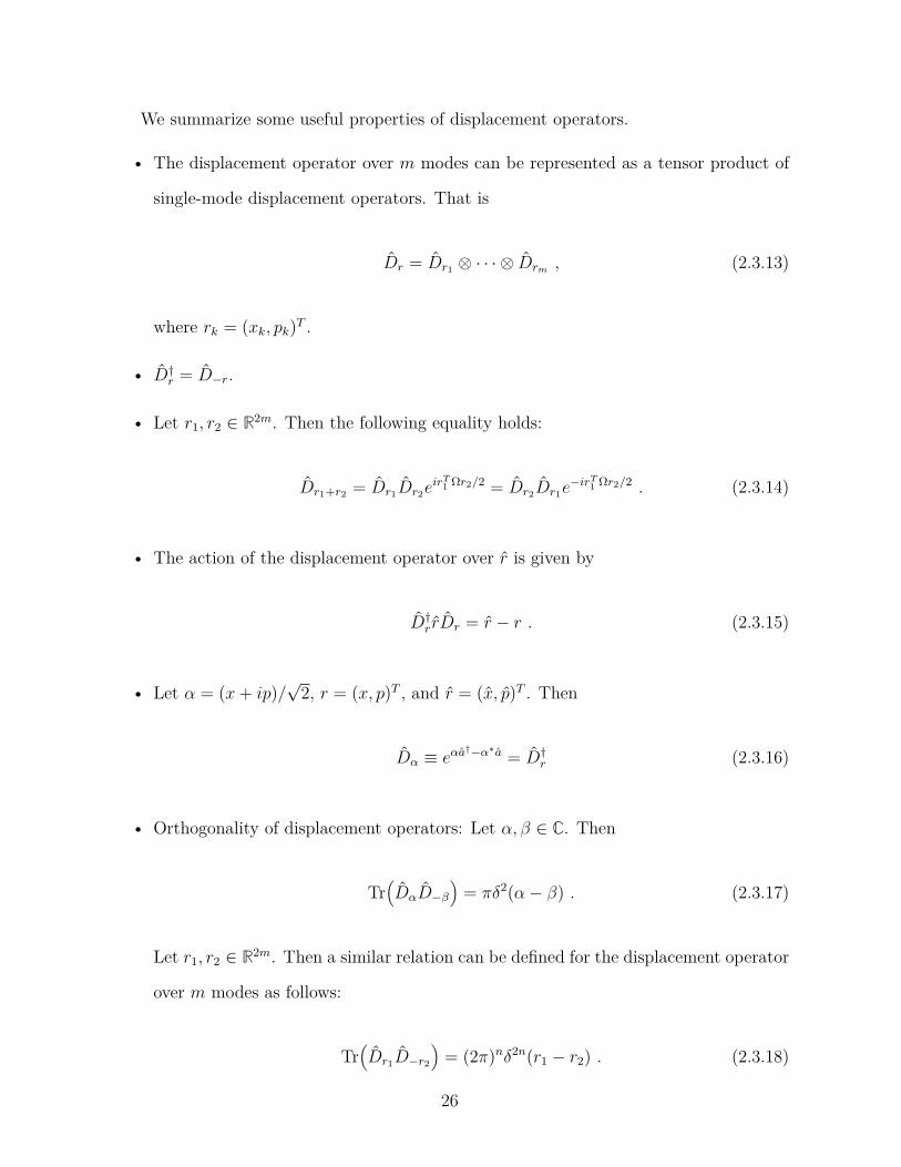
We summarize some useful properties of displacement operators.

• The displacement operator over m modes can be represented as a tensor product of

single-mode displacement operators. That is

Dr

= Dr1

⊗ · · · ⊗ Drm

,

(2.3.13)

where rk

= ( xk

, pk)T .

• D

†

r

= D− r.

• Let r1

, r2

∈ R2 m. Then the following equality holds:

Dr1+ r2

= Dr1

Dr2

eir

T

1

Ω r2

/ 2 = Dr2

Dr1

e− ir

T

1

Ω r2

/ 2 .

(2.3.14)

• The action of the displacement operator over ˆ r is given by

D

†

rˆ r Dr

= ˆ r − r .

(2.3.15)

• Let α = ( x + ip ) /√

2 , r = ( x, p )T , and ˆ r = (ˆ x, ˆ p )T . Then

Dα

≡ eα ˆ a† − α∗ˆ a = D

†

r

(2.3.16)

• Orthogonality of displacement operators: Let α , β ∈ C . Then

Tr

(

Dα

D− β

)

= π δ2( α − β ) .

(2.3.17)

Let r1

, r2

∈ R2 m. Then a similar relation can be defined for the displacement operator

over m modes as follows:

Tr

(

Dr1

D− r2

)

= (2 π )n δ2 n( r1

− r2) .

(2.3.18)

26

Definition 40 (Wigner characteristic function) Let r = ( x1

, p1

, . . . , xm

, pm)T . For

an m -mode quantum state ρ ∈ D ( H ) , the corresponding Wigner characteristic function is

defined as follows

χρ( r ) ≡ Tr( D

†

r

ρ ) .

(2.3.19)

Definition 41 (Fourier-Weyl relation) Let r = ( x1

, p1

, . . . , xm

, pm)T . Then every m -

mode quantum state can be represented in terms of the Wigner characteristic function as

follows

ρ =

1

(2 π )m

∫

dr χρ( r ) Dr

,

(2.3.20)

where dr = dx1

dp1

. . . dxm

dpm.

Definition 42 (Mean vector) Let ρ be an m -mode bosonic state. Then the mean vector

of ρ is defined as follows:

¯ r

ρ ≡ Tr( ρ ˆ r ) = (¯ x1

, ¯ p1

, . . . , ¯ xm

, ¯ pm)T ,

(2.3.21)

where ˆ r is given by (2.3.6) , ¯ xk

= Tr( ρ ˆ xk) and ¯ pk

= Tr( ρ ˆ pk) .

Thus the mean vector of an m -mode quantum state is a 2 m × 1 -dimensional vector.

Definition 43 (Covariance matrix) Let ρ be an m -mode bosonic state. Then the co-

variance matrix elements are defined as

σ

ρ

j k

≡ Tr

(

ˆ r

c

j

, ˆ r

c

k

ρ

)

(2.3.22)

where ˆ r

c

j

, ˆ r

c

k

= ˆ r

c

jˆ r

c

k

+ ˆ r

c

kˆ r

c

j

and ˆ r

c

j

= ˆ rj

− Tr(ˆ rj

ρ ) for all j , k ∈ 1 , . . . , 2 m , and ˆ r is given

by (2.3.6) .

Thus the covariance matrix of an m -mode quantum state is a 2 m × 2 m -dimensional

matrix.

Properties of a covariance matrix σ

ρ:

27

• The covariance matrix σ

ρ of a state ρ satisfies

σ

ρ + i Ω ≥ 0 ,

(2.3.23)

which is a manifestation of the uncertainty principle [115].

• The covariance matrix σ

ρ is positive definite, i.e, σ

ρ > 0 .

Definition 44 (Gaussian state) A quantum state ρ is Gaussian if its Wigner charac-

teristic function has a Gaussian form as

χρ( r ) = exp

(

−1

4

[Ω r ]T σ

ρΩ r + [Ω¯ r

ρ]T r

)

,

(2.3.24)

where ¯ r

ρ and σ

ρ are given by (2.3.21) and (2.3.22) , respectively.

Thus a bosonic Gaussian state ρ can be completely characterized by its mean vector ¯ r

ρ

and covariance matrix σ

ρ. We now discuss an alternate representation of faithful Gaussian

states.

Let us first define the most general quadratic Hamiltonian for m modes. Let H be

2 m × 2 m positive definite real matrix:

H =

1

2(ˆ r − ¯ r )T H (ˆ r − ¯ r ) ,

(2.3.25)

where ¯ r ∈ R2 m.

Then a faithful Gaussian state can be defined as the thermal state corresponding to

H , i.e.,

ρ =

e− H

Tr

(

e− H

) .

(2.3.26)

We now define a faithful Gaussian state ρ in terms of its mean vector and the covariance

matrix.

28

Definition 45 (Faithful Gaussian states) Let ρ denote an m -mode bosonic Gaussian

state. Let ¯ r

ρ and σ

ρ denote the mean vector and the covariance matrix of ρ , respectively.

If ρ is faithful, it can represented as follows:

ρ =

e− 1

2 (ˆ r − ¯ r

ρ)T H

′(ˆ r − ¯ r

ρ)

√

Det

(

σ

ρ+ i Ω

2

)

,

(2.3.27)

where

H

′ = S

T H S

H =

n⊕

j =1

ωj

1 0

0 1

(2.3.28)

with ωj

> 0 , ∀ j ∈ 1 , . . . , n , and S symplectic.

Thermal state . Let Hm

≡

∑m

j =1

ωjˆ a†

jˆ aj, where ωj

> 0 , ∀ j . Then a thermal Gaussian state

θβ

of m modes with respect to Hm

and having inverse temperature β > 0 thus has the

following form:

θβ

=

e− β Hm

Tr e− β Hm

,

(2.3.29)

and has a mean vector equal to zero and a diagonal 2 m × 2 m covariance matrix. One can

calculate that the mean photon number in this state is equal to

∑

j

1

eβ ωj − 1

.

(2.3.30)

A single-mode thermal state with mean photon number ¯ n = 1 / ( eβ ω − 1) has the following

representation in the photon number basis:

θ (¯ n ) ≡

1

1 + ¯ n

∞∑

n =0

( ¯ n

¯ n + 1

)n

| n ⟩⟨ n | .

(2.3.31)

It is also well known that thermal states can be written as a Gaussian mixture of displace-

29

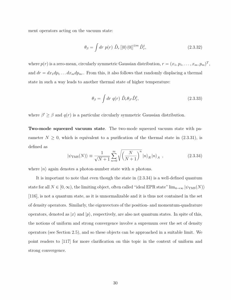
ment operators acting on the vacuum state:

θβ

=

∫

dr p ( r ) Dr

[ | 0 ⟩⟨ 0 | ]⊗ m D

†

r

,

(2.3.32)

where p ( r ) is a zero-mean, circularly symmetric Gaussian distribution, r = ( x1

, p1

, . . . , xm

, pm)T ,

and dr = dx1

dp1

. . . dxm

dpm.. From this, it also follows that randomly displacing a thermal

state in such a way leads to another thermal state of higher temperature:

θβ

=

∫

dr q ( r ) Dr

θβ

′ D

†

r

,

(2.3.33)

where β

′ ≥ β and q ( r ) is a particular circularly symmetric Gaussian distribution.

Two-mode squeezed vacuum state . The two-mode squeezed vacuum state with pa-

rameter N ≥ 0 , which is equivalent to a purification of the thermal state in (2.3.31), is

defined as

| ψTMS( N ) ⟩ ≡

1

√

N + 1

∞∑

n =0

√

(

N

N + 1

)n

| n ⟩R

| n ⟩A

,

(2.3.34)

where | n ⟩ again denotes a photon-number state with n photons.

It is important to note that even though the state in (2.3.34) is a well-defined quantum

state for all N ∈ [0 , ∞ ) , the limiting object, often called “ideal EPR state” lim¯ n →∞

| ψTMS( N ) ⟩

[116], is not a quantum state, as it is unnormalizable and it is thus not contained in the set

of density operators. Similarly, the eigenvectors of the position- and momentum-quadrature

operators, denoted as | x ⟩ and | p ⟩ , respectively, are also not quantum states. In spite of this,

the notions of uniform and strong convergence involve a supremum over the set of density

operators (see Section 2.5), and so these objects can be approached in a suitable limit. We

point readers to [117] for more clarification on this topic in the context of uniform and

strong convergence.

30

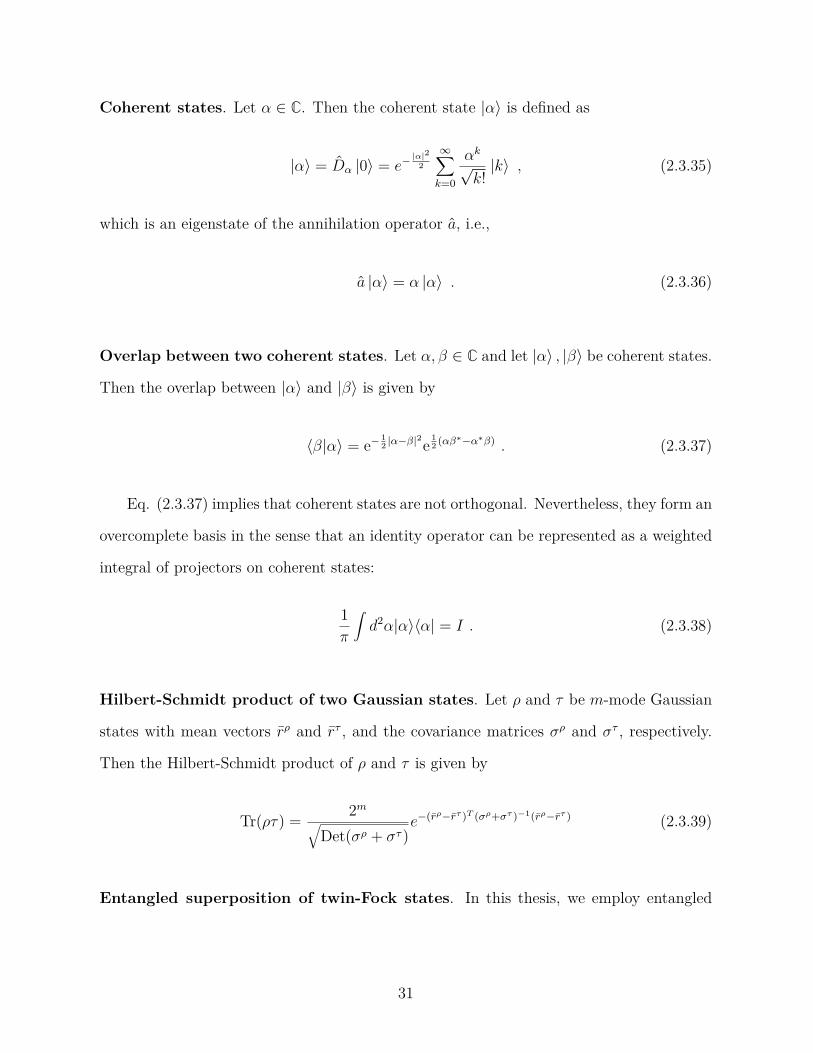
Coherent states . Let α ∈ C . Then the coherent state | α ⟩ is defined as

| α ⟩ = Dα

| 0 ⟩ = e−

| α |2

2

∞∑

k =0

α

k

√

k !

| k ⟩ ,

(2.3.35)

which is an eigenstate of the annihilation operator ˆ a , i.e.,

ˆ a | α ⟩ = α | α ⟩ .

(2.3.36)

Overlap between two coherent states . Let α , β ∈ C and let | α ⟩ , | β ⟩ be coherent states.

Then the overlap between | α ⟩ and | β ⟩ is given by

⟨ β | α ⟩ = e− 1

2

| α − β |2e

1

2 ( αβ

∗ − α∗ β ) .

(2.3.37)

Eq. (2.3.37) implies that coherent states are not orthogonal. Nevertheless, they form an

overcomplete basis in the sense that an identity operator can be represented as a weighted

integral of projectors on coherent states:

1

π

∫

d2 α | α ⟩⟨ α | = I .

(2.3.38)

Hilbert-Schmidt product of two Gaussian states . Let ρ and τ be m -mode Gaussian

states with mean vectors ¯ r

ρ and ¯ r

τ , and the covariance matrices σ

ρ and σ

τ , respectively.

Then the Hilbert-Schmidt product of ρ and τ is given by

Tr( ρτ ) =

2m

√

Det( σ

ρ + σ

τ )

e− (¯ r

ρ − ¯ r

τ )T ( σ

ρ+ σ

τ )− 1(¯ r

ρ − ¯ r

τ )

(2.3.39)

Entangled superposition of twin-Fock states . In this thesis, we employ entangled

31

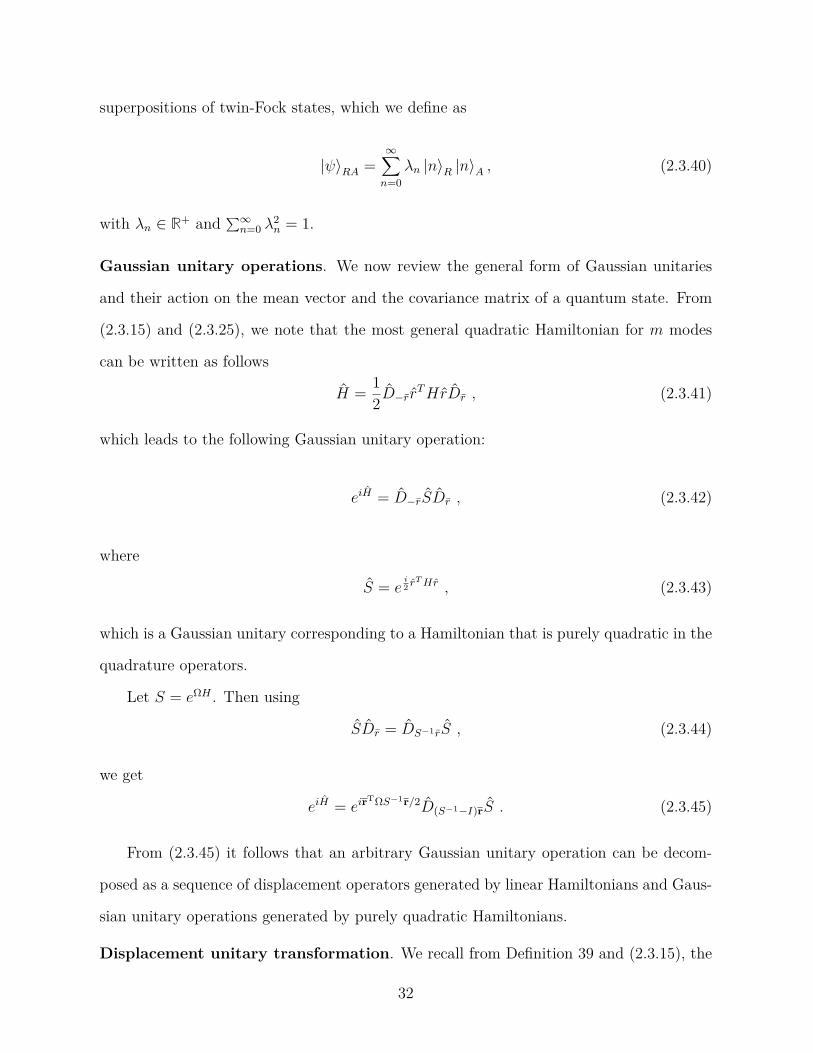
superpositions of twin-Fock states, which we define as

| ψ ⟩R A

=

∞∑

n =0

λn

| n ⟩R

| n ⟩A

, (2.3.40)

with λn

∈ R+ and

∑∞

n =0

λ2

n

= 1 .

Gaussian unitary operations . We now review the general form of Gaussian unitaries

and their action on the mean vector and the covariance matrix of a quantum state. From

(2.3.15) and (2.3.25), we note that the most general quadratic Hamiltonian for m modes

can be written as follows

H =

1

2

D− ¯ rˆ r

T H ˆ r D¯ r

,

(2.3.41)

which leads to the following Gaussian unitary operation:

ei H = D− ¯ r

S D¯ r

,

(2.3.42)

where

S = e

i

2 ˆ r

T H ˆ r ,

(2.3.43)

which is a Gaussian unitary corresponding to a Hamiltonian that is purely quadratic in the

quadrature operators.

Let S = eΩ H . Then using

S D¯ r

= DS

− 1¯ r

S ,

(2.3.44)

we get

ei H = ei

rTΩ S

− 1

r / 2 D( S

− 1 − I )

rS .

(2.3.45)

From (2.3.45) it follows that an arbitrary Gaussian unitary operation can be decom-

posed as a sequence of displacement operators generated by linear Hamiltonians and Gaus-

sian unitary operations generated by purely quadratic Hamiltonians.

Displacement unitary transformation . We recall from Definition 39 and (2.3.15), the

32

mean vector of a state ρ transforms as follows:

Tr

(

ˆ r D

†

r

ρ Dr

)

= ¯ r

ρ + r .

(2.3.46)

Thus the displacement operator only modifies the mean vector of ρ , and the covariance

matrix remains unchanged.

Symplectic transformation . Let S denote a Gaussian unitary corresponding to a Hamil-

tonian that is purely quadratic in the quadrature operators, such that S = e

i

2 ˆ r

T H ˆ r, where

H is a real positive definite matrix. Let us assume that the quantum state ρ transforms

under S as follows: S

† ρS . Then the mean vector ¯ r

ρ and the covariance matrix σ

ρ of the

state ρ transforms as follows:

¯ r

ρ → S ¯ r

ρ , (2.3.47)

σ

ρ → S σ

ρ S

T , (2.3.48)

where

S = eΩ H .

(2.3.49)

We now state the singular value decomposition of symplectic matrices, which further

simplifies the form of a symplectic matrix and equivalently of a symplectic unitary trans-

formation.

Singular value decomposition of symplectic matrices . Any 2 m × 2 m symplectic

matrix can be decomposed as

S = O Z O ,

(2.3.50)

where O and O are both symplectic and orthogonal matrices, and Z has the following form:

Z =

m⊕

j =1

zj

0

0 z

− 1

j

,

(2.3.51)

33

for zj

≥ 1 .

Beamsplitter . A beamsplitter consists of a semi-reflective mirror, which both partly

reflects and transmits the input radiation. In general the unitary operator corresponding

to the beamsplitter transformation is given by [26]

U

θ ,ϕ

BS

≡ exp

[

iθ ( eiϕˆ a†

inbin

+ e− iϕˆ ainb†

in)

]

,

(2.3.52)

where ˆ ain

and bin

denote the two incoming modes on either side of the beamsplitter, and θ

depends on the interaction time and coupling strength of semi-reflective mirrors. Moreover,

ϕ denotes the relative phase shift parameter. Another representation of a beamsplitter is

given in terms of the transmissivity η of the beamsplitter, where η = (cos θ )2. In this thesis,

we parametrize a beamsplitter with respect to η and θ interchangeably.

The symplectic matrix corresponding to the beamsplitter transformation is given by

SBS

=

cos θ 0 sin θ sin ϕ sin θ cos ϕ

0 cos θ − sin θ cos ϕ sin θ sin ϕ

− sin θ sin ϕ sin θ cos ϕ cos θ 0

− sin θ cos ϕ − sin θ sin ϕ 0 cos θ

,

(2.3.53)

which corresponds to an orthogonal symplectic transformation as in (2.3.50).

Phase rotations . The unitary operator corresponding to the phase rotation is given by

U

ϕ

PR

= exp( i ˆ nϕ ) ,

(2.3.54)

where ˆ n denotes the number operator. Moreover, the symplectic matrix corresponding to

34

the phase rotation unitary is given by

Sϕ

=

cos ϕ sin ϕ

− sin ϕ cos ϕ

.

(2.3.55)

which also corresponds to an orthogonal symplectic transformation as in (2.3.50).

Squeezer . A single-mode squeezer is a unitary operator defined as

S ( ξ ) ≡ exp

[

( ξ

∗ˆ a2 − ξ ˆ a† 2) / 2

]

, (2.3.56)

where ξ = r eiθ, with r ∈ [0 , ∞ ) and θ ∈ [0 , 2 π ] (see, e.g., [118] for a review). A squeezing

transformation realizes a decrement in the variance of one of the quadratures at the expense

of a corresponding increment in the variance of the complementary quadrature, which is

helpful for improving the sensitivity of an interferometer [119] and for other quantum

metrological tasks [118]. Let θ = 0 . Then the symplectic transformation corresponding to

S ( r ) is given by

SSQ

=

er 0

0 e− r

,

(2.3.57)

which we described as Z in (2.3.50).

SUM gate . A SUM gate is a quantum nondemolition (QND) interaction between two

modes and it is the CV analog of the CNOT gate [74]:

SUMG ≡ exp( − i G ˆ x1

⊗ ˆ p2) ,

(2.3.58)

where ˆ x1

and ˆ p2

correspond to the position- and momentum-quadrature operators of modes

1 and 2, respectively, and G is the gain of the interaction. Generally, G = 1 is sufficient for

quantum information processing tasks. This CV entangling quantum gate has applications

in CV quantum error correction [120,121] and CV coherent communication [122,123].

35

Let ρin

12

denote a two-mode input quantum state. Then the action of the ideal SUMG

gate on the mode operators ˆ x1, ˆ x2, ˆ p1, and ˆ p2

of ρin

12

is given by

ˆ xin

1

→ ˆ xin

1

, (2.3.59)

ˆ pin

1

→ ˆ pin

1

− G ˆ pin

2

, (2.3.60)

ˆ xin

2

→ ˆ xin

2

+ G ˆ xin

1

, (2.3.61)

ˆ pin

2

→ ˆ pin

2

. (2.3.62)

Gaussian channels . Quantum channels that take an arbitrary Gaussian input state to

another Gaussian state are called quantum Gaussian channels. Let N denote a Gaussian

channel that takes n modes to m modes. Then N transforms the Wigner characteristic

function χρ( r ) of a state ρ as follows:

χρ( r ) → χN ( ρ )( r ) = χρ

(

ΩT X

TΩ r

)

exp

(

−1

4

r

TΩT Y Ω r + ir

TΩT d

)

,

(2.3.63)

where X is a real 2 m × 2 n matrix, Y is a real 2 m × 2 m positive semi-definite symmetric

matrix, and d ∈ R2 m, such that they satisfy the following condition for N to be a physical

channel:

Y + i Ω − iX Ω X

T ≥ 0 .

(2.3.64)

Furthermore, since a Gaussian state ρ can be completely characterized by its mean vector

¯ r

ρ and covariance matrix σ

ρ, the action of a Gaussian channel on ρ can be described as

follows:

¯ r

ρ → X ¯ r

ρ + d ,

σ

ρ → X σ

ρ X

T + Y . (2.3.65)

36

Just as every quantum channel can be implemented as a unitary transformation acting

on a larger space followed by a partial trace, so can Gaussian channels be implemented

as a Gaussian unitary on a larger space with some extra modes prepared in the vacuum

state, followed by a partial trace [124]. Given a Gaussian channel NX ,Y

with Z such that

Y = Z Z

T we can find two other matrices XE

and ZE

such that there is a symplectic matrix

S =

X Z

XE

ZE

,

(2.3.66)

which corresponds to a Gaussian unitary transformation on a larger space. The comple-

mentary channel N XE

,YE

from input to the environment then effects the following trans-

formation on mean vectors and covariance matrices:

µρ 7−→ XE

µρ , (2.3.67)

V

ρ 7−→ XE

V

ρ X

T

E

+ YE

, (2.3.68)

where YE

≡ ZE

Z

T

E .

Displacement covariance . All Gaussian channels are covariant with respect to displace-

ment operators. Let NX ,Y

denote a Gaussian channel with X and Y matrices. Then the

following relation holds

NX ,Y ( Dr

ρD

†

r) = DX r

NX ,Y ( ρ ) D

†

X r

,

(2.3.69)

and note that DX r

is a tensor product of local displacement operators.

Phase-insensitive bosonic channels . A channel N is phase insensitive or phase covari-

ant if

N ( e− i ˆ nϕ ρei ˆ nϕ) = e− i ˆ nϕ N ( ρ ) ei ˆ nϕ

(2.3.70)

for all ϕ ∈ R and input states ρ ∈ D ( H ) .

A phase-insensitive, single-mode bosonic Gaussian channel adds an equal amount of

37

noise to each quadrature of the electromagnetic field, such that

X = diag(√

τ ,

√

τ ) , (2.3.71)

Y = diag( ν , ν ) , (2.3.72)

d = 0 , (2.3.73)

where τ ∈ [0 , 1] corresponds to attenuation, τ ≥ 1 amplification, and ν is the variance of

an additive noise. Moreover, the following inequalities should hold

ν ≥ 0 , (2.3.74)

ν2 ≥ (1 − τ )2 , (2.3.75)

in order for the map to be a legitimate completely positive and trace preserving map. The

channel is entanglement breaking [125] if the following inequality holds [126]

ν ≥ τ + 1 .

(2.3.76)

We now provide examples of phase-insensitive, bosonic Gaussian channels.

Quantum thermal channel . A quantum thermal channel is a phase-insensitive Gaussian

channel that can be characterized by a beamsplitter of transmissivity η ∈ (0 , 1) , coupling

the signal input state with a thermal state with mean photon number NB

≥ 0 , and followed

by a partial trace over the environment. Let B

η

AE

denote a beamsplitter with transmissivity

η ∈ (0 , 1) . Let θ ( NB) denote a thermal state with mean photon number NB. Then the

action of a thermal channel Lη ,NB

A → B

with the transmissivity parameter η and the thermal

noise parameter NB

is defined as

Lη ,NB

A → B( ρA) ≡ Tr E( B

η

AE( ρA

⊗ θE( NB))) ,

(2.3.77)

38

for all input states ρA.

In the Heisenberg picture, the beamsplitter transformation is given by the following

Bogoliubov transformation:

b =

√

η ˆ a −

√

1 − η ˆ e, (2.3.78)

ˆ e′ =

√

1 − η ˆ a +

√

η ˆ e, (2.3.79)

where ˆ a, b , ˆ e , and ˆ e′ are the annihilation operators representing the sender’s input mode,

the receiver’s output mode, an environmental input mode, and an environmental output

mode of the channel, respectively. If the mean photon number at the input of a thermal

channel is no larger than NS, then the total number of photons that make it through the

channel to the receiver is no larger than η NS

+ (1 − η ) NB.

Pure-loss channel . A thermal channel is called a pure-loss channel if the thermal state in

the environment mode has mean photon number NB

= 0 . Let Lη

A → B

with the transmissivity

parameter η denote a pure-loss channel. Then from (2.3.77) we get

Lη

A → B( ρA) ≡ Tr E( B

η

AE( ρA

⊗ | 0 ⟩⟨ 0 |E)) ,

(2.3.80)

where | 0 ⟩⟨ 0 |E

denotes the vacuum state in the mode E . Throughout this thesis, we denote

a pure-loss channel by Lη and Lη , 0 interchangeably.

Quantum amplifier channel A quantum amplifier channel is a Gaussian channel that

can be characterized by a two-mode squeezer with parameter G > 1 , coupling the signal

input state with a thermal state with mean photon number NB

≥ 0 , and followed by a

partial trace over the environment. Let ΞG

AE

denote a two-mode squeezer with G > 1 .

Then the action of a quantum amplifier channel AG,NB on a state ρA

is given by

AG,NB

A → B( ρA) ≡ Tr E(ΞG

AE( ρA

⊗ θE( NB)) ,

(2.3.81)

39

where again θE( NB) denotes a thermal state with mean photon number NB.

In the Heisenberg picture, the two-mode squeezer implementing a quantum amplifier

channel has the following Bogoliubov transformation:

b =

√

G ˆ a +

√

G − 1ˆ e† , (2.3.82)

ˆ e′ =

√

G − 1ˆ a† +

√

G ˆ e , (2.3.83)

where ˆ a, b , ˆ e , and ˆ e′ correspond to the same parties as discussed above.

Quantum limited amplifier . When NB

= 0 , the quantum amplifier channel is called the

quantum limited amplifier channel. In other words, a quantum limited amplifier channel

AG

A → B

with the gain parameter G is defined as

AG

A → B( ρA) ≡ Tr E(ΞG

AE( ρA

⊗ | 0 ⟩⟨ 0 |E)) , (2.3.84)

where | 0 ⟩⟨ 0 |E

again denotes the vacuum state in the mode E . Throughout this thesis, we

denote a quantum-limited amplifier channel by AG and AG, 0 interchangeably.

Additive-noise channel . An additive-noise channel is specified by the following com-

pletely positive and trace preserving map:

T

ξ

A → B( ρ ) ≡

∫

d2 α Pξ( α ) Dα

ρD

†

α

,

(2.3.85)

where Pξ

= exp( −| α |2 /ξ ) / ( π ξ ) and Dα

is a displacement operator for the input mode.

The variance ξ > 0 completely characterizes the channel T

ξ, and it roughly represents the

number of noise photons added to the input mode by the channel.

From [127, 128], it follows that an additive-noise channel T

ξ

A → B

can be expressed as a

concatenation of a pure-loss channel Lη

A → B

′

with transmissivity η followed by a quantum-

40

limited amplifier channel A1 /η

B

′ → B

with gain parameter 1 /η ,

T

ξ

A → B

= A1 /η

B

′ → B

Lη

A → B

′

(2.3.86)

with ξ = (1 − η ) /η .

Joint phase covariance . Let N and M be quantum channels that take one input mode

to m output modes. Then N and M are jointly phase covariant if the following holds:

NA → B

(

ei ˆ nϕ ρe− i ˆ nϕ

)

=

(

m⊗

i =1

ei ˆ ni( − 1)ai ϕ

)

NA → B( ρ )

(

m⊗

i =1

e− i ˆ ni( − 1)ai ϕ

)

,

MA → B

(

ei ˆ nϕ ρe− i ˆ nϕ

)

=

(

m⊗

i =1


)

MA → B( ρ )

(

m⊗

i =1


)

,

(2.3.87)

where ai

∈ 0 , 1 for i ∈ 1 , . . . , m , and ˆ ni

is the number operator in the i th mode.

Homodyne measurement . A homodyne measurement is a Gaussian channel to measure

the quadrature operator

ˆ xϕ

= cos ϕ ˆ x + sin ϕ ˆ p ,

(2.3.88)

and the corresponding probability of outcome is given by

p ( xϕ) = Tr( | xϕ

⟩⟨ xϕ

| ρ ) ,

(2.3.89)

where | xϕ

⟩ is an improper eigenvector of ˆ xϕ.

Photodetection . Let P denote the channel corresponding to the ideal photodetector,

whose action on an input state ρ is defined as follows:

P ( ρ ) ≡

∞∑

n =0

⟨ n | ρ | n ⟩| n ⟩⟨ n | .

(2.3.90)

The interpretation of this channel is that it measures the input state in the photon-number

basis and then outputs the measured value in a classical register.

Throughout this thesis, we consider only those quantum channels that satisfy the fol-

41

lowing finite output entropy condition:

Condition 46 (Finite output entropy) Let G be a Gibbs observable and W ∈ [0 , ∞ ) .

A quantum channel N satisfies the finite-output entropy condition with respect to G and

W if

sup

ρ : Tr Gρ ≤ W

H ( N ( ρ )) < ∞ ,

(2.3.91)

2.4 Distance Measures for Quantum States and Channels

This section defines several distance measures relevant for the rest of the thesis. We

begin by defining the trace distance, the fidelity, and the sine distance between two density

operators. We then introduce the distance measures for distinguishing quantum channels.

Finally, we present the notion of energy-constrained distance measures.

Definition 47 (Trace distance) The trace distance between two operators A, B ∈ L ( H , H

′)

is defined as follows:

∥ A − B ∥1

.

(2.4.1)

The trace distance between two quantum states ρ, σ ∈ D ( H ) is an operationally relevant

distance measure. In particular, consider the following hypothesis testing scenario: suppose

that Alice prepares one of two quantum states ρ and σ , and suppose that it is equally likely

a priori for her to prepare either ρ or σ . Furthermore, suppose that Bob can perform a

binary POVM to distinguish ρ and σ . Then the maximum success probability to distinguish

is linearly related to the normalized trace distance as follows:

psucc

=

1

2

(

1 +

1

2

∥ ρ − σ ∥1

)

.

(2.4.2)

We will later invoke the following important properties of the trace distance between

ρ and σ :

42

• Isometric invariance : Let U denote an isometry. Then the trace distance is invari-

ant with respect to an isometric quantum operation as follows:

∥ ρ − σ ∥1

= ∥ U ρU

† − U σ U

† ∥1

.

(2.4.3)

• Triangle inequality : For any three quantum states ρ, σ, ω ∈ D ( H ) , the following

inequality holds:

∥ ρ − ω ∥1

≤ ∥ ρ − σ ∥1

+ ∥ σ − ω ∥1

.

(2.4.4)

• Monotonicity : Let NA → B

denote a quantum channel. Let ρ, σ ∈ D ( HA) . Then the

trace distance is monotone with respect to the action of the channel N :

∥N ( ρ ) − N ( σ ) ∥1

≤ ∥ ρ − σ ∥1

.

(2.4.5)

An alternate measure of the closeness of two quantum states is the fidelity, which we

define below.

Definition 48 (Fidelity) The fidelity between ρ and σ is defined as follows [129]:

F ( ρ, σ ) ≡

∥∥∥√

ρ√

σ

∥∥∥

2

1

.

(2.4.6)

Similar to the trace distance, the fidelity between two quantum states satisfies impor-

tant properties, which we summarize below.

• Multiplicativity : The fidelity is multiplicative with respect to tensor products:

F ( ρA

⊗ ρB

, σA

⊗ σB) = F ( ρA

, σA) F ( ρB

, σB) ,

(2.4.7)

where ρA

, σA

∈ D ( HA) and ρB

, σB

∈ D ( HB) .

• Isometric invariance : Let U denote an isometry. Let ρ, σ ∈ D ( H ) . Then the

43

following holds:

F ( ρ, σ ) = F ( U ρU

† , U σ U

†) .

(2.4.8)

• Monotonicity : Let NA → B

denote a quantum channel. Let ρ, σ ∈ D ( HA) . Then the

fidelity is monotone with respect to the action of the channel N :

F ( ρ, σ ) ≤ F ( N ( ρ ) , N ( σ )) .

(2.4.9)

• Joint concavity of the root fidelity : Let pX

denote a probability distribution.

Let ρx

, σx

∈ D ( H ) for all x . Then the root fidelity is jointly concave with respect to

its input arguments:

√

F

(∑

x

pX( x ) ρx

,

∑

x

pX( x ) σx

)

≥

∑

x

pX( x )

√

F ( ρx

, σx) .

(2.4.10)

Definition 49 (Sine distance) The sine distance between two density operators ρ, σ ∈

D ( H ) is defined as [130–133]

C ( ρ, σ ) ≡

√

1 − F ( ρ, σ ) .

(2.4.11)

Definition 50 (Relation between fidelity and trace distance) The following inequal-

ities relate the fidelity and the trace distance [134]:

1 −

√

F ( ρ, σ ) ≤

1

2

∥ ρ − σ ∥1

≤

√

1 − F ( ρ, σ ) ,

(2.4.12)

with the lower bound following from the Powers-Størmer inequality [135] and the upper

bound from Uhlmann’s theorem [129]. See also [134].

The notions of trace distance and fidelity can be extended to distinguish two quantum

operations. We begin by defining the diamond norm of a Hermiticity preserving linear

44

map.

Definition 51 (Diamond norm) Let SA → B

denote a Hermiticity preserving linear map.

Then the diamond norm of S is defined as

∥S ∥⋄

≡ sup

ρR A

∈D ( HR

⊗HA)

∥ ( IR

⊗ SA → B)( ρR A) ∥1

,

(2.4.13)

where IR

is the identity map acting on a Hilbert space HR

corresponding to an arbitrarily

large reference system [136].

From the convexity of the trace norm (2.1.10) and the Schmidt decomposition theorem

as in Definition 14, it suffices to optimize with respect to input states ρ that are pure. A

distance measure to distinguish two quantum operations can be defined as follows based

on the diamond norm.

Definition 52 (Diamond distance) Let NA → B

and MA → B

denote quantum channels.

Then the diamond distance is defined as

∥N − M∥⋄

≡ sup

ρR A

∈D ( HR

⊗HA)

∥ ( IR

⊗ NA → B)( ρR A) − (idR

⊗MA → B)( ρR A) ∥1

,

(2.4.14)

where IR

is the identity map acting on a Hilbert space HR.

Similar to the trace distance between two quantum states, the diamond distance is an

operationally relevant distance measure to distinguish two quantum channels. Consider the

following hypothesis testing task: suppose that Alice can implement one of two quantum

channels N and M . Bob prepares a state ρR A

and sends system A to Alice. Then Alice

flips a fair coin and, based on the outcome, applies either N or M , and then sends the

output system B to Bob. Finally, Bob measures systems R and B to figure out which

channel Alice applied. In such a scenario, the maximum success probability to distinguish

N and M is linearly related to the normalized diamond-norm distance between N and M

45

as follows:

psucc

=

1

2

(

1 +

1

2

∥N − M∥⋄

)

(2.4.15)

Definition 53 (Channel fidelity) Let NA → B

and MA → B

denote quantum channels. The

channel fidelity between N and M is defined as

F ( N , M ) ≡ inf

ρR A

∈D ( HR

⊗HA)

F (( IR

⊗ NA → B)( ρR A) , ( IR

⊗ MA → B)( ρR A)) ,

(2.4.16)

where IR

is the identity map acting on a Hilbert space HR.

From joint concavity of root fidelity and monotonicity of the square function, the

optimization in (2.4.16) can be reduced to pure states in HR A.

Definition 54 (Energy-constrained diamond distance) Let HA

denote a Hamilto-

nian corresponding to the quantum system A . Let NA → B

and MA → B

be two quantum

channels. Let R denote a reference system. Then the energy-constrained diamond distance

between NA → B

and MA → B

is defined for E ∈ [0 , ∞ ) as [137,138]

∥NA → B

− MA → B

∥⋄ E

≡ sup

ρR A:Tr( HA

ρA) ≤ E

∥NA → B( ρR A) − MA → B( ρR A) ∥1

,

(2.4.17)

where ρR A

∈ D ( HR A) , and it is implicit that the identity channel IR

acts on system R .

From the convexity of the trace norm and the Schmidt decomposition theorem, it

suffices to optimize (2.4.17) with respect to input states ρR A

that are pure and satisfy the

energy constraint Tr( HA

ρA) ≤ E . Moreover, we note that due to the supremum being

taken, the diamond norm might only be achieved in the limit (for example, for a sequence

of two-mode squeezed vacuum states with squeezing strength becoming arbitrarily large,

as discussed in [117]).

Definition 55 (Energy-constrained channel fidelity) The energy-constrained channel

fidelity between two quantum channels NA → B

and MA → B

for E ∈ [0 , ∞ ) is defined as

46

[93,139]

FE( NA → B

, MA → B) ≡ inf

ρR A:Tr( HA

ρA) ≤ E

F ( NA → B( ρR A) , MA → B( ρR A)) ,

(2.4.18)

ρR A

∈ D ( HR

⊗ HA) , and again it is implicit that the identity channel IR

acts on system R .

Definition 56 (Energy-constrained sine distance) The energy-constrained sine dis-

tance between two quantum channels NA → B

and MA → B

for E ∈ [0 , ∞ ) is defined as

[93,139]

CE( NA → B

, MA → B) ≡ sup

ρR A:Tr( HA

ρA) ≤ E

√

1 − F ( NA → B( ρR A) , MA → B( ρR A)) .

(2.4.19)

For both the energy-constrained channel fidelity and the energy-constrained sine dis-

tance between two quantum channels N and M , it is sufficient to optimize over pure input

states ρR A

∈ D ( HR A) satisfying the energy constraint.

Definition 57 (Relation between (2.4.17) and (2.4.18) ) Similar to Definition 50, we

have the following relation between the energy-constrained channel fidelity and the energy-

constrained diamond distance:

1 −

√

FE( NA → B

, MA → B) ≤

1

2

∥NA → B

− MA → B

∥⋄ E

≤ CE( NA → B

, MA → B) ,

(2.4.20)

where NA → B

and MA → B

are quantum channels, E ∈ [0 , ∞ ) , and CE( NA → B

, MA → B) is

given by (2.4.19) .

2.5 Notions of Convergence for Quantum Channels

In this section, we briefly summarize three different notions of convergence for quantum

channels: uniform and strong convergence (as presented in [140]), and uniform convergence

on the set of density operators whose marginals on the channel input have bounded energy

47

(as presented in [137, 138]). Uniform and strong convergence in the context of infinite-

dimensional quantum channels were studied in [140]. A connection between the notion of

strong convergence and the notion of uniform convergence over energy-bounded states was

established in [137]. Later, these different topologies of convergence were studied in the

context of linear bosonic channels and Gaussian dilatable channels in [141]. Furthermore,

topologies of convergence in the context of teleportation simulation of physically relevant

phase-insensitive bosonic Gaussian channels have been investigated in [117].

We first recall the notion of uniform convergence for quantum channels.

Definition 58 (Uniform convergence) Let Mk

A → B

k

denote a sequence of quantum

channels, where each channel takes a trace-class operator acting on a separable Hilbert

space HA

to a trace-class operator acting on a separable Hilbert space HB. Then the channel

sequence Mk

A → B

k

converges uniformly to another quantum channel NA → B

if the following

holds:

lim

k →∞

∥∥∥ Mk

A → B

− NA → B

∥∥∥⋄

= 0 .

(2.5.1)

Qualitatively, the uniform convergence of a sequence of quantum channels to another

quantum channel implies that the convergence is independent of the input state.

Definition 59 (Strong convergence) Let Mk

A → B

k

denote a sequence of quantum chan-

nels, where each channel takes a trace-class operator acting on a separable Hilbert space

HA

to a trace-class operator acting on a separable Hilbert space HB. Then the channel

sequence Mk

A → B

k

converges to another quantum channel NA → B

in the strong sense if for

all ψR A

∈ D ( HR

⊗ HA) , the following holds:

lim

k →∞

∥∥∥ Mk

A → B( ψR A) − NA → B( ψR A)

∥∥∥1

= 0 ,

(2.5.2)

which can be summarized more compactly as

sup

ψR A

∈D ( HR A)

lim

k →∞

∥∥∥ Mk

A → B( ψR A) − NA → B( ψR A)

∥∥∥1

= 0 .

(2.5.3)

48

Here, it is implicit that the identity channel acts on the reference system R .

Therefore, convergence in the strong sense is the statement that, for each fixed input quan-

tum state ψR A, the sequence Mk

A → B( ψR A) k

of states converges to the state NA → B( ψR A)

in trace norm. It is important to note that the different orders in which the limits and

suprema are taken in (2.5.1) and (2.5.3) lead to physically distinct situations, as discussed

in [117]. Moreover, one can infer from the definitions of strong and uniform convergence

that the notion of strong convergence is a weaker notion of convergence, in fact implied by

uniform convergence.

Definition 60 (Bounded energy uniform convergence) Let HA

denote an energy ob-

servable corresponding to the quantum system A . Then the channel sequence Mk

A → B

k

converges uniformly (on the set of density operators whose marginals on the channel input

have bounded energy) to another quantum channel NA → B

if the following holds for some

E ∈ [0 , ∞ ) :

lim

k →∞

∥∥∥ Mk

A → B

− NA → B

∥∥∥⋄ E

= 0 .

(2.5.4)

We note that the strong convergence of a sequence of infinite-dimensional channels is

equivalent to uniform convergence on the set of energy-bounded density operators [137].

2.6 Approximate Degradability of Quantum Channels

The concept of approximate degradability was introduced in [66]. The following two

definitions of approximate degradability will be useful in our thesis.

Definition 61 ( ε -degradable [66]) A channel NA → B

is ε -degradable if there exists a

channel DB → E

such that

1

2

∥∥∥ N − D N

∥∥∥⋄

≤ ε ,

(2.6.1)

where N denotes a complementary channel of N .

49

Definition 62 ( ε -close-degradable [66]) A channel NA → B

is ε -close-degradable if there

exists a degradable channel MA → B

such that

1

2

∥N − M∥⋄

≤ ε .

(2.6.2)

Remark 63 Let NA → B

be a quantum channel that is ε -close-degradable. Then NA → B

is

ε + 2√

ε -degradable by [66, Proposition A.5]. A converse implication is not known to hold.

Remark 64 The notion of ε -degradable and ε -close degradable quantum channels was de-

fined in [66] for finite-dimensional channels. In this thesis, we generalize it to infinite-

dimensional channels by replacing the diamond norm in (2.6.1) and (2.6.2) with the energy-

constrained diamond norm.

2.7 Quantum Channel Capacities

The energy-constrained quantum and private capacities of quantum channels have been

defined in [62, Section III]. In what follows, we review the definition of quantum commu-

nication and private communication codes, achievable rates, and regularized formulas for

energy-constrained quantum and private capacities.

Energy-constrained quantum capacity : An ( n, M , G, W, ε ) code for energy-constrained

quantum communication consists of an encoding channel E

n : T ( HS) → T ( H

⊗ n

A

) and a

decoding channel D

n : T ( H

⊗ n

B

) → T ( HS) , where M = dim( HS) . The energy constraint is

such that the following bound holds for all states resulting from the output of the encoding

channel E

n:

Tr

Gn

E

n( ρS) ≤ W ,

(2.7.1)

where ρS

∈ D ( HS) . Note that

Tr

Gn

E

n( ρS)

= Tr G

ρn

,

(2.7.2)

50

where

ρn

≡

1

n

n∑

i =1

TrAn \ Ai

E

n( ρS) .

(2.7.3)

due to the i.i.d. nature of the observable

Gn. Furthermore, the quantum communication

code satisfies the following reliability condition such that for all pure states ϕR S

∈ D ( HR

⊗

HS) ,

F ( ϕR S

, (idR

⊗ [ D

n N

⊗ n E

n])( ϕR S)) ≥ 1 − ε ,

(2.7.4)

where HR

is isomorphic to HS. A rate R is achievable for quantum communication over

N subject to the energy constraint W if for all ε ∈ (0 , 1) , δ > 0 , and sufficiently large n ,

there exists an ( n, 2n [ R − δ ] , G, W, ε ) energy-constrained quantum communication code. The

energy-constrained quantum capacity Q ( N , G, W ) of N is equal to the supremum of all

achievable rates.

If the channel N satisfies Condition 46 and G is a Gibbs observable, then the quantum

capacity Q ( N , G, W ) is equal to the regularized energy-constrained coherent information

of the channel N [62]

Q ( N , G, W ) = limn →∞

1

n

Ic( N

⊗ n ,

Gn

, W ) ,

(2.7.5)

where the energy-constrained coherent information of the channel is defined as [62]

Ic( N , G, W ) ≡ sup

ρ :Tr ρG ≤ W

H ( N ( ρ )) − H ( N ( ρ )) ,

(2.7.6)

and N denotes a complementary channel of N . Note that another definition of energy-

constrained quantum communication is possible, but it leads to the same value for the

capacity in the asymptotic limit of many channel uses [62].

Energy-constrained private capacity. An ( n, M , G, W, ε ) code for private communica-

tion consists of a set ρm

An

M

m =1

of quantum states, each in D ( H

⊗ n

A

) , and a POVM Λm

B

n

M

m =1

51

such that

Tr

Gn

ρm

An

≤ W, (2.7.7)

Tr Λm

B

n

N

⊗ n( ρm

An) ≥ 1 − ε, (2.7.8)

1

2

∥∥∥ N

⊗ n( ρm

An) − ωE

n

∥∥∥1

≤ ε, (2.7.9)

for all m ∈ 1 , . . . , M , with ωE

n some fixed state in D ( H

⊗ n

E

) . In the above, N is a channel

complementary to N . A rate R is achievable for private communication over N subject

to energy constraint W if for all ε ∈ (0 , 1) , δ > 0 , and sufficiently large n , there exists an

( n, 2n [ R − δ ] , G, W, ε ) private communication code. The energy-constrained private capacity

P ( N , G, W ) of N is equal to the supremum of all achievable rates.

An upper bound on the energy-constrained private capacity of a channel has been

established in [62], but the lower bound still needs a detailed proof. However, the results

in [62] suggest the validity of the following form. If the channel N satisfies Condition 46

and G is a Gibbs observable, then the energy-constrained private capacity P ( N , G, W ) is

given by the regularized energy-constrained private information of the channel:

P ( N , G, W ) = limn →∞

1

n

P (1)( N

⊗ n ,

Gn

, W ) ,

(2.7.10)

where the energy-constrained private information is defined as

P (1)( N , G, W ) ≡ sup

¯ ρEA:Tr G ¯ ρEA

≤ W

∫

dx pX( x )[ D ( N ( ρx

A) ∥N (¯ ρEA)) − D ( N ( ρx

A) ∥ N (¯ ρEA))] ,

(2.7.11)

¯ ρEA

≡

∫

dx pX( x ) ρx

A

is an average state of the ensemble

EA

≡ pX( x ) , ρx

A

,

(2.7.12)

and N denotes a complementary channel of N . Note that another definition of energy-

52

constrained private communication is possible, but it leads to the same value for the ca-

pacity in the asymptotic limit of many channel uses [62].

Remark 65 The unconstrained quantum and private capacities of a quantum channel N

are defined in the same way as above, but without the energy constraints demanded in (2.7.1)

and (2.7.7) . As a consequence of these definitions and the fact that the set of states with

finite but arbitrarily large energy is dense in the set of all states, for channels satisfying the

finite output-entropy condition for every energy W ≥ 0 , the unconstrained quantum and

private capacities are respectively given by

sup

W ≥ 0

Q ( N , G, W ) , sup

W ≥ 0

P ( N , G, W ) .

(2.7.13)

2.8 Continuity of Information Quantities and Channel Capacities

In this section, we recall continuity bounds for the conditional quantum entropy with

energy constraints and for capacities of quantum channels. We also derive a theorem on

the continuity of output entropy for infinite-dimensional systems with finite average energy

constraints.

2.8.1 Continuity of Conditional Quantum Entropy

The following lemma is a uniform continuity bound for the conditional quantum entropy

with energy constraints [114]:

Lemma 1 (Meta-Lemma 17, [114]) For a Gibbs observable G ∈ P ( HA) , and states

ωAB

, τAB

∈ D ( HA

⊗ HB) , such that

1

2

∥ ωAB

− τAB

∥1

≤ ε < ε′ ≤ 1 , Tr ( G ⊗ IB) ωAB

,

Tr ( G ⊗ IB) τAB

≤ W , where W ∈ [0 , ∞ ) and δ = ( ε′ − ε ) / (1+ ε′) , the following inequality

holds

| H ( A | B )ω

− H ( A | B )τ

| ≤ (2 ε′ + 4 δ ) H ( γ ( W /δ )) + g ( ε′) + 2 h2( δ ) .

(2.8.1)

53

2.8.2 Continuity of Output Entropy

The following theorem on continuity of output entropy for infinite-dimensional systems

with finite average energy constraints is a direct consequence of [142, Theorem 11] and

Lemma 1.

Theorem 66 Let NA → B

and MA → B

be quantum channels, G ∈ P ( HB) be a Gibbs observ-

able, such that

Tr

Gn

N

⊗ n( ρAn) , Tr

Gn

M⊗ n( ρAn) ≤ W ,

(2.8.2)

where W ∈ [0 , ∞ ) and ρR An ∈ D ( HR

⊗ H

⊗ n

A

) . If

1

2

∥N − M∥⋄

≤ ε < ε′ ≤ 1 and δ =

( ε′ − ε ) / (1 + ε′) , then the following inequality holds

∣∣∣ H ((idR

⊗N

⊗ n

A → B)( ρR An)) − H ((idR

⊗M⊗ n

A → B)( ρR An))

∣∣∣

≤ n [(2 ε′ + 4 δ ) H ( γ ( W /δ )) + g ( ε′) + 2 h2( δ )] . (2.8.3)

Proof. Let

ρj = (idR

⊗M⊗ j

A → B

⊗ N

⊗ ( n − j )

A → B

)( ρR An) ,

(2.8.4)

54

and consider the following chain of inequalities:

| H ( R B

n)ρ0 − H ( R B

n)ρn |

=

∣∣∣∣∣∣

n∑

j =1

H ( R B

n)ρj − 1 − H ( R B

n)ρj

∣∣∣∣∣∣

(2.8.5)

≤

n∑

j =1

∣∣∣ H ( R B

n)ρj − 1 − H ( R B

n)ρj

∣∣∣ (2.8.6)

=

n∑

j =1

∣∣∣ H ( Bj

| R B1

· · · Bj − 1

Bj +1

· · · Bn)ρj − 1 − H ( Bj

| R B1

· · · Bj − 1

Bj +1

· · · Bn)ρj

∣∣∣ (2.8.7)

≤ n [(2 ε′ + 4 δ )

n∑

j =1

1

n

H ( γ ( Wj

/δ ))

+ g ( ε′) + 2 h2( δ )] (2.8.8)

≤ n [(2 ε′ + 4 δ ) H

1

n

n∑

j =1

γ ( Wj

/δ )

+ g ( ε′) + 2 h2( δ )] (2.8.9)

≤ n [(2 ε′ + 4 δ ) H ( γ ( W /δ )) + g ( ε′) + 2 h2( δ )] . (2.8.10)

The first inequality follows from the triangle inequality. The second equality follows from

the fact that the states ρj and ρj − 1 are the same except for the j th output system. Let

Wj

denote an energy constraint on the j th output state of both the channels N and M ,

i.e., Tr G N ( ρAj) , Tr G M ( ρAj

) ≤ Wj

and

1

n

∑

j

Wj

≤ W . Then the second inequality

follows because

1

2

∥ ρj − ρj − 1 ∥1

≤ ε for the given channels, and we use Lemma 1 for the j th

output system. The third inequality follows from concavity of entropy. The final inequality

follows because

Tr

1

n

n∑

j =1

G γ ( Wj

/δ )

=

1

n

n∑

j =1

Tr G γ ( Wj

/δ ) ≤ W /δ,

(2.8.11)

and γ ( W /δ ) is the Gibbs state that maximizes the entropy corresponding to the energy

W /δ .

55

2.8.3 Continuity of Capacities for Channels

The continuity of various capacities of quantum channels has been discussed in [142,

Lemma 12]. The general form for the classical, quantum, or private capacity of a channel N

can be defined as F ( N ) = lim n →∞

1

n

supP ( n )

fn( N

⊗ n , P ( n )) , where fn

n

denotes a family of

functions, and P ( n ) represents states or parameters over which an optimization is performed.

Then the following lemma holds [142].

Lemma 2 (Lemma 12, [142]) If F ( N ) = lim n →∞

1

n

supP ( n )

fn( N

⊗ n , P ( n )) for a channel

N and ∀ n, P ( n ),

∣∣∣ fn( N

⊗ n , P ( n )) − fn( M⊗ n , P ( n ))

∣∣∣ ≤ nc , then | F ( N ) − F ( M ) | ≤ c .

2.9 Karush-Kuhn-Tucker (KKT) Conditions

In this section, we review the Karush-Kuhn-Tucker (KKT) conditions used in solving

convex optimization problems with inequality constraints. We will invoke these conditions

in Chapter 5 to solve quadratic programs.

Let x ∈ Rn and let f : Rn → R . Consider the following primal optimization problem:

min

x ∈ Rn

f ( x )

subject to ui( x ) ≤ 0 , ∀ i ∈ 1 , . . . , k

vj( x ) = 0 , ∀ j ∈ 1 , . . . , l

(2.9.1)

Let L ( x, a, b ) denote a Lagrangian with the following form:

L ( x, a, b ) ≡ f ( x ) +

k∑

i =1

ai

ui( x ) +

l∑

j =1

bj

vj( x ) , (2.9.2)

where a ≡ ( a1

, . . . , ak) and b ≡ ( b1

, . . . , bl) , and ai

, bi

∈ R .

Using the Lagrange dual function:

g ( a, b ) ≡ min

x ∈ Rn

L ( x, a, b ) , (2.9.3)

the dual problem corresponding to the optimization in (2.9.1) can be defined as follows

56

(see [143] for a review):

max

a,b

g ( a, b )

subject to ai

≥ 0 , ∀ i ∈ 1 , . . . , k ,

(2.9.4)

where b ∈ Rl.

Let ˜ x denote a primal feasible point and let (˜ a, b ) denote a dual feasible point. Then

it is easy to show that f (˜ x ) ≥ g (˜ a, b ) , which is the weak duality condition. To see this,

consider the following chain of inequalities:

g (˜ a, b ) = min

x ∈ Rn

f ( x ) +

k∑

i =1

˜ ai

ui( x ) +

l∑

j =1

bj

vj( x ) (2.9.5)

≤ f (˜ x ) +

k∑

i =1

˜ ai

ui(˜ x ) +

l∑

j =1

bj

vj(˜ x ) (2.9.6)

≤ f (˜ x ) . (2.9.7)

The first equality follows from (2.9.2) and (2.9.3). The first inequality follows due to the

minimization over all x ∈ Rn in (2.9.5). Since ˜ x is a primal feasible point, it satisfies

vj(˜ x ) = 0 , ∀ j and ui(˜ x ) ≤ 0 , ∀ i . Moreover, since ˜ a is a dual feasible point, ˜ ai

≥ 0 , ∀ i .

Collectively, these conditions imply that

∑k

i =1

˜ ai

ui(˜ x ) ≤ 0 and

∑l

j =1 bj

vj(˜ x ) = 0 , which

leads to the last inequality.

The duality gap f (˜ x ) − g (˜ a, b ) provides a way to bound how suboptimal primal and

dual feasible points are. Let f

∗ denote the primal optimal value and g

∗ the dual optimal

value. Then the following inequalities hold:

f (˜ x ) − f

∗ ≤ f (˜ x ) − g

∗ ≤ f (˜ x ) − g (˜ a, b ) , (2.9.8)

which follow from the weak duality condition in (2.9.7) and from the definitions of the

57

primal and dual optimal values. Thus we get

f

∗ ∈ [ f (˜ x ) , g (˜ a, b )] and g

∗ ∈ [ f (˜ x ) , g (˜ a, b )] , (2.9.9)

which implies that the optimality of f (˜ x ) and g (˜ a, b ) depend on the the duality gap. In

other words, if the duality gap is zero, ˜ x is a primal optimal point and (˜ a, b ) is a dual

optimal point.

We now describe the KKT conditions for the aforementioned optimization problem,

which are necessary conditions in the sense that if a primal optimal point x∗ and a dual

optimal point ( a∗ , b∗) with zero duality gap exist, they satisfy the KKT conditions. We

later will argue when the KKT conditions are also sufficient for the optimality of a solution.

The KKT conditions are given by

Stationarity condition ∂x

L ( x, a, b ) |x∗ = 0

Complementary slackness a∗

i

ui( x∗) = 0 , ∀ i ∈ 1 , . . . , k

Primal feasibility ui( x∗) ≤ 0 , ∀ i ∈ 1 , . . . , k

vj( x∗) = 0 , ∀ j ∈ 1 , . . . , l

Dual feasibility a∗

i

≥ 0 , ∀ i ∈ 1 , . . . , k

(2.9.10)

We provide a brief proof for why primal and dual optimal points with zero duality

gap satisfy the KKT conditions. First note that if x∗ is a primal optimal solution, then it

satisfies the primal feasibility conditions, as a consequence of (2.9.1). Similarly, if ( a∗ , b∗)

is a dual optimal solution, then as a consequence of (2.9.4), it satisfies the dual feasibility

condition. Moreover, the zero duality gap implies that inequalities in (2.9.5)–(2.9.7) should

be saturated. Therefore, the primal optimal point x∗ minimizes L ( x, a∗ , b∗) , which implies

that the partial derivative of L ( x, a∗ , b∗) at x = x∗ is equal to zero. In other words, the

58

stationarity condition is satisfied. Finally, the zero duality gap further implies that

∑

i

a∗

i

ui( x∗) = 0 .

(2.9.11)

Since a∗

i

ui( x∗) ≤ 0 , ∀ i ∈ 1 , . . . , k , from (2.9.11) we get that a∗

i

ui( x∗) = 0 , ∀ i . Thus the

complementary slackness is satisfied. This completes the proof.

In our work, we solve an optimization problem in which f ( x ) is a convex quadratic

function in x , and ui( x ) and vj( x ) are linear in x . Thus the Lagrangian in (2.9.2) is

a convex function in x . We now argue that for such optimization problems, the KKT

conditions are both necessary and sufficient. Suppose that ¯ x and (¯ a, b ) satisfy the KKT

conditions. Then from the stationarity condition in (2.9), we get ∂x

L ( x, ¯ a, b ) |¯ x

= 0 . Since

L ( x, ¯ a, b ) is convex in x , we get min x

L ( x, ¯ a, b ) = L (¯ x, ¯ a, b ) . Therefore, from (2.9.3), it

follows that

g (¯ a, b ) = f (¯ x ) +

k∑

i =1

¯ ai

ui(¯ x ) +

l∑

j =1

bj

vj(¯ x ) = f (¯ x ) ,

(2.9.12)

where the last equality follows from KKT conditions, i.e., ¯ ai

ui(¯ x ) = 0 , ∀ i and vj(¯ x ) = 0 , ∀ j .

Thus the zero duality gap in (2.9.12) implies that ¯ x and (¯ a, b ) are respectively primal and

dual optimal solutions, as argued in (2.9.9).

59

CHAPTER 3

BOUNDING THE ENERGY-CONSTRAINED QUANTUM

AND PRIVATE CAPACITIES OF PHASE-INSENSITIVE

BOSONIC GAUSSIAN CHANNELS

In this chapter we motivate the importance of energy-constrained distinguishabil-

ity measures in estimating the ultimate communication capabilities of bosonic Gaussian

quantum channels. In particular, we focus on particular phase-insensitive Gaussian chan-

nels: thermal, amplifier, and additive-noise channels. In general, these channels are non-

degradable bosonic Gaussian channels and hence getting a good estimate of quantum and

private capacities is a computationally challenging problem.

Before providing a detailed summary of our results, let us motivate why our results

imply that the energy-constrained distinguishability measures can help in establishing tight

upper bounds on the quantum and private capacities of bosonic channels. One of the bounds

on the capacities of a thermal channel, as established in this chapter, is based on the notion

of an ε -degradable quantum channel, as in Definition 61. In particular, this bound relies on

the energy-constrained diamond distance between two particular Gaussian channels. We

find that for certain parameter (e.g., mean-energy value of the channel inputs, thermal

noise parameter, etc.) regimes, in comparison to all other upper bounds established in

this chapter, the bound based on the ε -degradability is closest to a known lower bound.

Thus, better estimates of the energy-constrained diamond distance can further improve our

understanding of quantum and private capacities of thermal channels.

Inspired from these findings, we will develop numerical and analytical tools to estimate

energy-constrained distance measures between Gaussian channels in Chapters 4 and 5.

We now provide a detailed summary of the results presented in this chapter.

Summary of results . We start by summarizing our upper bounds on the energy-

constrained quantum capacity of thermal channels. A first upper bound is established

60

by decomposing a thermal channel as a pure-loss channel followed by a quantum-limited

amplifier channel [127,128] and using a data-processing argument. We note that the same

method was employed in [144], in order to establish an upper bound on the classical ca-

pacity of the thermal channel (note that the general idea for the data-processing argument

comes from the earlier work in [145, 146]). Throughout, we call this first upper bound the

“data-processing bound.” We also prove that this upper bound can be at most 1.45 bits

larger than a known lower bound [64,147] on the energy-constrained quantum and private

capacity of a thermal channel. Moreover, the data-processing bound is very near to a

known lower bound for the case of low thermal noise and both low and high transmissivity.

The notion of approximate degradability of quantum channels was developed in [66],

and upper bounds on the quantum and private capacities of approximately degradable

channels were established for quantum channels with finite-dimensional input and output

systems. In this dissertation, we establish general upper bounds on the energy-constrained

quantum and private capacities of approximately degradable channels for infinite-dimensional

systems. These general upper bounds can be applied to any quantum channel that is ap-

proximately degradable with energy constraints on the input and output states of the

channels. In particular, we apply these general upper bounds to bosonic Gaussian thermal

and amplifier channels. In Chapter 5, we summarize how these general upper bounds can

be applied to bosonic additive-noise channels.

Our second upper bound is based on the notion of ε -degradability of thermal channels,

and we call this bound the “ ε -degradable bound.” In this method, we first construct a

degrading channel, such that a complementary channel of the thermal channel is close

in diamond distance [136] to the serial concatenation of the thermal channel followed by

this degrading channel. In general, it seems to be computationally hard to determine

the diamond distance between two quantum channels if the optimization is over input

density operators acting on an infinite-dimensional Hilbert space. However, in our setup,

we address this difficulty by constructing a simulating channel, which simulates the serial

61

concatenation of the thermal channel and the aforementioned degrading channel. Using

this technique, an upper bound on the diamond distance reduces to the calculation of

the quantum fidelity between the environmental states of the thermal channel and the

simulating channel. Based on the fact that, for certain parameter regimes, the resulting

capacity upper bound is better than all other upper bounds reported here, we believe that

our aforementioned choice of a degrading channel is a good choice.

A third upper bound on the energy-constrained quantum capacity of thermal channels

is established using the concept of ε -close-degradability of a thermal channel, and we call

this bound the “ ε -close-degradable bound.” In particular, we show that a low-noise thermal

channel is ε -close degradable, given that it is close in diamond distance to a pure-loss

channel. We find that the ε -close-degradable bound is very near to the data-processing

bound for the case of low thermal noise.

We then prove that any phase-insensitive channel that is not entanglement-breaking

[125] can be decomposed as the concatenation of a quantum-limited amplifier channel

followed by a pure-loss channel. This theorem was independently proven in [148, 149] (see

also [150]). It has been used to bound the unconstrained quantum capacity of a thermal

channel in [148], via a data-processing argument. We use this technique to prove an upper

bound on the energy-constrained quantum and private capacities of a thermal channel.

This technique has also been used most recently in [149] in similar contexts, as well as

in [151]. In particular, we find that this upper bound is very near to a known lower bound

for the case of low thermal noise and both low and high transmissivity. We call this bound

the “bottleneck bound.” We find that the bottleneck bound and the data-processing bound

are incomparable, as one is better than the other for certain parameter regimes.

We compare these different upper bounds with a known lower bound on the quantum

capacity of a thermal channel [64,147]. We find that the data-processing and the bottleneck

bounds are very near to a known capacity lower bound for low thermal noise and for both

medium and high transmissivity. Moreover, we show that the maximum difference between

62

the data-processing bound and a known lower bound never exceeds 1 / ln 2 ≈ 1 . 45 bits for

all possible values of parameters, and this maximum difference is attained in the limit of

infinite input mean photon number. This result places a strong limitation on any possible

superadditivity of coherent information of the thermal channel. We note here that this kind

of result was suggested without proof by the heuristic developments in [152]. Next, we plot

these upper bounds as well as a known lower bound versus input mean photon number for

different values of the channel transmissivity η and thermal noise NB. In particular, we

find that the ε -close-degradable bound is very near to the data-processing bound for low

thermal noise and for both medium and high transmissivity. Moreover, all of these upper

bounds are very near to a known lower bound for low thermal noise and high transmissivity.

We also examine different parameter regimes where the ε -close-degradable bound is tighter

than the ε -degradable bound and vice versa. In particular, we find that the ε -degradable

bound is tighter than the ε -close degradable bound for the case of high thermal noise.

We find an interesting parameter regime where the ε -degradable bound is tighter than

all other upper bounds, as it becomes closest to a known lower bound for the case of high

noise and high input mean photon number. However, for the same parameter regime, if the

input mean photon number is low, then the data-processing bound is tighter than the ε -

degradable bound. This suggests that the upper bounds based on the notion of approximate

degradability are good for the case of high input mean photon number. We suspect that

these bounds could be further improved for the case of low input mean photon number

if it were possible to compute or tightly bound the energy-constrained diamond norm

[137, 138] (see also Section 3.8 for some developments in this direction). In Chapter 4 we

develop techniques to estimate the energy-constrained diamond distance between quantum

channels. In particular, we introduce the notion of energy-constrained diamond distance on

a truncated input Hilbert space in (4.1.38), which can be calculated using a semi-definite

program, as described in (4.1.67). This serves as a numerical tool to approximate the

energy-constrained diamond norm with an arbitrarily high accuracy (see Proposition 116

63

for more details).

Similar to our bounds on the energy-constrained quantum capacity, we establish several

upper bounds on the energy-constrained private capacity of bosonic thermal channels. We

also develop an improved lower bound on the energy-constrained private capacity of a

bosonic thermal channel. In particular, we find that for certain values of the channel

transmissivity, a higher private communication rate can be achieved by using displaced

thermal states as information carriers instead of coherent states.

Related to our bounds on energy-constrained quantum and private capacities of thermal

channels, we establish several upper bounds on the same capacities of quantum amplifier

channels. We also establish upper bounds on the energy-constrained quantum and private

capacities of an additive-noise channel.

As one of the last technical developments of this chapter, we address the question of

computing energy-constrained channel distances in a very broad sense, by considering the

energy-constrained, generalized channel divergence of two quantum channels, as an exten-

sion of the generalized channel divergence developed in [153]. In particular, we prove that

an optimal Gaussian input state for the energy-constrained, generalized channel divergence

of two particular Gaussian channels is the two-mode squeezed vacuum state that saturates

the energy constraint. It is an interesting open question to determine whether the two-

mode squeezed vacuum is optimal among all input states, but we leave this for future work,

simply noting for now that an answer would lead to improved upper bounds on the energy-

constrained quantum and private capacities of the thermal and amplifier channels. At the

least, we have proven that the optimal input state for the particular Gaussian channels is

such that its reduction to the channel input system is diagonal in the photon number basis.

Moreover, in Chapter 5 we prove that two-mode squeezed vacuum state is not optimal

among all input states if one compares an additive-noise channel to an identity channel

with respect to energy-constrained channel fidelity.

The rest of the chapter is structured as follows. We provide general upper bounds

64

on the energy-constrained quantum and private capacities of approximately degradable

channels in Section 3.1. We use these tools to establish several upper bounds on the energy-

constrained quantum and private capacities of a thermal channel in Sections 3.2 and 3.4,

respectively. A comparision of these different upper bounds on energy-constrained quantum

capacity of a thermal channel is discussed in Section 3.3. We present an improvement on

the achievable rate of private communication through thermal channels, in Section 3.5. We

establish bounds on energy-constrained capacities of a quantum amplifier channel and an

additive-noise channel in Sections 3.6 and 3.7, respectively. We discuss the optimization of

the Gaussian energy-constrained generalized channel divergence in Section 3.8. Finally, we

summarize our results and conclude in Section 3.9.

3.1 Bounds on Energy-Constrained Quantum and Private Capacities of Ap-

proximately degradable channels

In this section, we derive upper bounds on the energy-constrained quantum and pri-

vate capacities of approximately degradable channels. We derive these bounds for both

ε -degradable (Definition 61) and ε -close-degradable (Definition 62) channels. This general

form for the upper bounds on the energy-constrained quantum and private capacities of

approximately degradable channels will be directly used in establishing bounds on the ca-

pacities of quantum thermal channels and amplifier channels. We also briefly summarize

how to obtain the ε -close-degradable bound for an additive-noise channel.

We begin by defining the conditional entropy of degradation , which will be useful for

finding upper bounds on the energy-constrained quantum and private capacities of an ε -

degradable channel. A similar quantity has been defined for the finite-dimensional case

in [66].

Definition 67 (Conditional entropy of degradation) Let NA → B

and DB → E

be quan-

tum channels, and let G ∈ P ( HA) be a Gibbs observable. We define the conditional entropy

65

of degradation as follows:

UD( N , G, W ) = sup

ρ : Tr Gρ ≤ W[ H ( N ( ρ )) − H ( D N ( ρ ))] ,

(3.1.1)

where W ∈ [0 , ∞ ) . For a Stinespring dilation V : T ( B ) → T ( E F ) of the channel D ,

UD( N , G, W ) = sup

ρ : Tr Gρ ≤ W[ H ( F | E )V N ( ρ )] .

(3.1.2)

We note that the conditional entropy of degradation can be understood as the negative

entropy gain of the channel DB → E

[154–157], with the optimization over input states N ( ρ )

restricted to the image of N and obeying the energy constraint Tr Gρ ≤ W . Next, we

show that the conditional entropy of degradation in (3.1.2) is additive.

Lemma 3 Let NA → B

and DB → E

be quantum channels, let G ∈ P ( HA) be a Gibbs observ-

able, and let W ∈ [0 , ∞ ) . Then for all integer n ≥ 1 ,

UD

⊗ n( N

⊗ n ,

Gn

, W ) = n [ UD( N , G, W )] .

(3.1.3)

Proof. The following inequality

UD

⊗ n( N

⊗ n ,

Gn

, W ) ≥ n [ UD( N , G, W )]

(3.1.4)

follows trivially because a product input state is a particular state of the form required in

the optimization of UD

⊗ n( N

⊗ n ,

Gn

, W ) . We now prove the less trivial inequality

UD

⊗ n( N

⊗ n ,

Gn

, W ) ≤ n [ UD( N , G, W )] .

(3.1.5)

66

Consider the following chain of inequalities:

H ( F

n | E

n)( V

⊗ n N

⊗ n)( ρAn )

≤

n∑

i =1

H ( Fi

| Ei)( V N )( ρAi)

(3.1.6)

≤ n [ H ( F | E )( V N )(¯ ρn)] (3.1.7)

≤ n [ UD( N , G, W )] , (3.1.8)

where ¯ ρn

=

1

n

∑n

i =1

ρAi. The first inequality follows from several applications of strong

subadditivity [158, 159]. The second inequality follows from concavity of conditional en-

tropy [158, 159]. The last inequality follows because Tr

Gn

ρAn = Tr G ¯ ρn

≤ W and the

conditional entropy of degradation UD( N , G, W ) involves an optimization over all input

states obeying this energy constraint. Since the chain of inequalities is true for all input

states ρAn satisfying the input energy constraint, the desired result follows.

3.1.1 Bound on the Energy-Constrained Quantum Capacity of an ε -Degradable

Channel

An upper bound on the quantum capacity of an ε -degradable channel was established

as [66, Theorem 3.1(ii)] for the finite-dimensional case. Here, we prove a related bound for

the infinite-dimensional case with finite average energy constraints on the input and output

states of the channels.


be an ε -degradable channel with a degrading channel DB → E

′, and

let G ∈ P ( HA) and G′ ∈ P ( HE

′) be Gibbs observables, such that for all input states

ρAn ∈ D ( H

⊗ n

A

) satisfying input average energy constraints Tr

Gn

ρAn ≤ W , the following

output average energy constraints are satisfied:

Tr

G

′

n

N

⊗ n( ρAn) , Tr

G

′

n( D

⊗ n N

⊗ n)( ρAn) ≤ W

′ ,

(3.1.9)

where NA → E

is a complementary channel of N and E

′ ≃ E . Then the energy-constrained

67

quantum capacity Q ( N , G, W ) is bounded from above as

Q ( N , G, W ) ≤ UD( N , G, W ) + (2 ε′ + 4 δ ) H ( γ ( W

′ /δ )) + g ( ε′) + 2 h2( δ ) ,

(3.1.10)

with ε′ ∈ ( ε, 1] , W, W

′ ∈ [0 , ∞ ) , and δ = ( ε′ − ε ) / (1 + ε′) .

Proof. Let

σB

n = N

⊗ n( ρAn) ,

ρj

E

′ j E( n − j )

= ( D

⊗ j N

⊗ j) ⊗ N

⊗ ( n − j )( ρAn) ,

and consider the following chain of inequalities:

H ( B

n)σ

− H ( E

n)ρ0

= H ( B

n)σ

− H ( E

′ n)ρn + H ( E

′ n)ρn − H ( E

n)ρ0 (3.1.11)

≤ UD

⊗ n( N

⊗ n ,

Gn

, W ) + H ( E

′ n)ρn − H ( E

n)ρ0 (3.1.12)

= n UD( N , G, W )

+

n∑

j =1

[ H ( E

′

j

| E

′

1

. . . E

′

j − 1

Ej +1

. . . En)ρj − H ( Ej

| E

′

1

. . . E

′

j − 1

Ej +1

. . . En)ρj − 1 ] (3.1.13)

≤ n [ UD( N , G, W ) + (2 ε′ + 4 δ )

n∑

j =1

1

n

H ( γ ( W

′

j

/δ ))

+ g ( ε′) + 2 h2( δ )] (3.1.14)

≤ n [ UD( N , G, W ) + (2 ε′ + 4 δ ) H

1

n

n∑

j =1

γ ( W

′

j

/δ )

+ g ( ε′) + 2 h2( δ )] (3.1.15)

≤ n [ UD( N , G, W ) + (2 ε′ + 4 δ ) H ( γ ( W

′ /δ )) + g ( ε′) + 2 h2( δ )] , (3.1.16)

The first inequality follows from the definition in (3.1.1). The second equality follows from

Lemma 3 and the telescoping technique. Let W

′

j

denote the energy constraint on the j th

output state of both the channels D N and N , i.e.,

Tr G′( D N )( ρAj) , Tr G′ N ( ρAj

) ≤ W

′

j

,

(3.1.17)

68

where

1

n

∑

j

W

′

j

≤ W

′. Then the second inequality holds because

1

2

∥ ρj − ρj − 1 ∥1

≤ ε for

the given channels, and we use Lemma 1 for the j th output system. The third inequality

follows from concavity of entropy. The last inequality follows because

Tr

1

n

n∑

j =1

Gγ ( W

′

j

/δ )

=

1

n

n∑

j =1

Tr Gγ ( W

′

j

/δ ) ≤ W

′ /δ ,

(3.1.18)

and γ ( W

′ /δ ) is the Gibbs state that maximizes the entropy corresponding to the energy

W

′ /δ . Since the chain of inequalities is true for all ρAn satisfying the input average energy

constraint, from (2.7.6) and the above, we get that

1

n

Ic( N

⊗ n ,

Gn

, W ) ≤ UD( N , G, W ) + (2 ε′ + 4 δ ) H ( γ ( W

′ /δ )) + g ( ε′) + 2 h2( δ ) .

(3.1.19)

Since the last inequality holds for all n , we obtain the desired result by taking the limit

n → ∞ and applying (2.7.5).

3.1.2 Bound on the Energy-Constrained Quantum Capacity of an ε -Close-

Degradable Channel

An upper bound on the quantum capacity of an ε -close-degradable channel was estab-

lished as [66, Proposition A.2(i)] for the finite-dimensional case. Here, we provide a bound

for the infinite-dimensional case with finite average energy constraints on the input and

output states of the channels.


be an ε -close-degradable channel, i.e.,

1

2

∥N − M∥⋄

≤ ε < ε′ ≤ 1 ,

where MA → B

is a degradable channel. Let G ∈ P ( HA) , G′ ∈ P ( HB) be Gibbs observables,

such that for all input states ρR An ∈ D ( HR

⊗ H

⊗ n

A

) satisfying the input average energy

constraint Tr

Gn

ρAn ≤ W , the following output average energy constraints are satisfied:

Tr

G

′

n

N

⊗ n( ρAn) , Tr

G

′

n

M⊗ n( ρAn) ≤ W

′ ,

(3.1.20)

where W, W

′ ∈ [0 , ∞ ) . Then the energy-constrained quantum capacity Q ( N , G, W ) is

69

bounded from above as

Q ( N , G, W ) ≤ Ic( M , G, W ) + (4 ε′ + 8 δ ) H ( γ ( W

′ /δ )) + 2 g ( ε′) + 4 h2( δ ) ,

(3.1.21)

with ε′ ∈ ( ε, 1] and δ = ( ε′ − ε ) / (1 + ε′) .

Proof. Let ωR B

n = (idR

⊗N

⊗ n)( ρR An) and τR B

n = (idR

⊗M⊗ n)( ρR An) , and consider the

following chain of inequalities:

H ( B

n)ω

− H ( R B

n)ω

− H ( B

n)τ

+ H ( R B

n)τ

= H ( B

n)ω

− H ( B

n)τ

+ H ( R B

n)τ

− H ( R B

n)ω

(3.1.22)

≤ 2 n [(2 ε′ + 4 δ ) H ( γ ( W /δ )) + g ( ε′) + 2 h2( δ )] , (3.1.23)

The first inequality follows from applying Theorem 66 twice. Then from Lemma 2,

Q ( N , G, W ) ≤ Q ( M , G, W ) + (4 ε′ + 8 δ ) H ( γ ( W

′ /δ )) + 2 g ( ε′) + 4 h2( δ ) .

(3.1.24)

The desired result follows from the fact that the energy-constrained quantum capacity

of a degradable channel is equal to the energy-constrained coherent information of the

channel [62].

3.1.3 Bound on the Energy-Constrained Private Capacity of an ε -Degradable

Channel

In this section, we first derive an upper bound on the private capacity of an ε -degradable

channel for the finite-dimensional case, which is different from any of the bounds presented

in [66]. Then, we generalize this bound to the infinite-dimensional case with finite average

energy constraints on the input and output states of the channels.


be a finite-dimensional ε -degradable channel with a degrading

channel DB → E

′, and let N : T ( A ) → T ( E ) be a complementary channel of N , such that

70

E

′ ≃ E . If

UD( N ) = max

ρ ∈D ( HA)[ H ( N ( ρ )) − H (( D N )( ρ ))] ,

(3.1.25)

then the private capacity P ( N ) of N is bounded from above as

P ( N ) ≤ UD( N ) + 6 ε log2 dim( HE) + 3 g ( ε ) .

(3.1.26)

Proof. Consider Stinespring dilations U : T ( A ) → T ( B E ) and V : T ( B ) → T ( E

′ F ) of the

channel N and the degrading channel D , respectively. Let ρX An be a classical–quantum

state in correspondence with an ensemble pX( x ) , ρx

An

:

ρX An =

∑

x

pX( x ) | x ⟩⟨ x |X

⊗ ρx

An

,

(3.1.27)

and let

ωX E

n E

′ n F

n =

∑

x

pX( x ) | x ⟩⟨ x |X

⊗ (id⊗ n

E

⊗V

⊗ n) U

⊗ n( ρx

An) .

(3.1.28)

Consider the following extension of ωX E

n E

′ n F

n :

σX Y E

n E

′ n F

n =

∑

x,y

pX( x ) pY | X( y | x ) | x ⟩⟨ x |X

⊗ | y ⟩⟨ y |Y

⊗ (id⊗ n

E

⊗V

⊗ n) U

⊗ n( ψ

x,y

An ) ,

(3.1.29)

71

where ψ

x,y

An

is a pure state, and let σ

x,y

E

n E

′ n F

n

= (id⊗ n

E

⊗V

⊗ n) U

⊗ n( ψ

x,y

An ) . Consider the

following chain of inequalities:

I ( X ; B

n)ω

− I ( X ; E

n)ω

= I ( X ; F

n | E

′ n)ω

+ I ( X ; E

′ n)ω

− I ( X ; E

n)ω

(3.1.30)

= I ( X ; F

n | E

′ n)ω

+ H ( E

′ n)ω

− H ( E

n)ω

+ H ( E

n | X )ω

− H ( E

′ n | X )ω

(3.1.31)

≤ I ( X ; F

n | E

′ n)ω

+ 2 n [2 ε log2 dim( HE) + g ( ε )] (3.1.32)

≤ I ( X Y ; F

n | E

′ n)σ

+ n [4 ε log2 dim( HE) + 2 g ( ε )] (3.1.33)

= H ( F

n | E

′ n)σ

− H ( F

n E

′ n | X Y )σ

+ H ( E

′ n | X Y )σ

+ n [4 ε log2 dim( HE) + 2 g ( ε )] (3.1.34)

= H ( F

n | E

′ n)σ

− H ( E

n | X Y )σ

+ H ( E

′ n | X Y )σ

+ n [4 ε log2 dim( HE) + 2 g ( ε )] (3.1.35)

≤ n [ UD( N ) + 6 ε log2 dim( HE) + 3 g ( ε )] . (3.1.36)

The first two equalities follow from entropy identities. The first inequality follows by ap-

plying the telescoping technique twice and using the continuity result of the conditional

quantum entropy for finite-dimensional quantum systems [114]. The second inequality

follows from the quantum data processing inequality for conditional quantum mutual in-

formation. The last two equalities follow from entropy identities and by using that σ

x,y

E

n E

′ n F

n

is a pure state, so that H ( F

n E

′ n)σ

x,y = H ( E

n)σ

x,y . The last inequality follows from the def-

inition in (3.1.25), and additivity of UD( N ) [66]. Also, we applied the telescoping technique

for each σ

x,y in the summation, and used the continuity result of the conditional quantum

entropy for finite-dimensional systems [114]. Since the chain of inequalities is true for any

ensemble pX( x ) , ρx

An

, the final result follows from the definition of private information

of the channel, dividing by n , taking the limit n → ∞ , and noting that the regularized

private information is equal to the private capacity of any channel.

72

Next, we derive an upper bound on the energy-constrained private capacity of an ε -

degradable channel.


be an ε -degradable channel with a degrading channel DB → E

′, and

let G ∈ P ( HA) , G′ ∈ P ( HE

′) be Gibbs observables, such that for all input states ρAn ∈

D ( H

⊗ n

A

) satisfying input average energy constraints Tr

Gn

ρAn ≤ W , the following output

average energy constraints are satisfied:

Tr

G

′

n

N

⊗ n( ρAn) , Tr

G

′

n( D

⊗ n N

⊗ n)( ρAn) ≤ W

′ ,

(3.1.37)

where NA → E

is a complementary channel of N , and E

′ ≃ E . Then the energy-constrained

private capacity is bounded from above as

P ( N , G, W ) ≤ UD( N , G, W ) + (6 ε′ + 12 δ ) H ( γ ( W

′ /δ )) + 3 g ( ε′) + 6 h2( δ ) ,

(3.1.38)

with ε′ ∈ ( ε, 1] , W, W

′ ∈ [0 , ∞ ) , and δ = ( ε′ − ε ) / (1 + ε′) .

Proof. Since the proof is similar to the above one and previous ones, we just summarize it

briefly below. Consider Stinespring dilations U : T ( A ) → T ( B E ) and V : T ( B ) → T ( E

′ F )

of the channel N and the degrading channel D , respectively. Then the action of U

⊗ n

followed by V

⊗ n on the ensemble pX( x ) , ρx

An

leads to the following ensemble:

pX( x ) , ω

x

E

n E

′ n F

n

≡ (id⊗ n

E

⊗V

⊗ n) U

⊗ n( ρx

An) .

(3.1.39)

Similar to the above proof, from applying the telescoping technique three times and using

Lemma 1, concavity of entropy, and Lemma 3, we get the following bound:

I ( X ; B

n)ω

− I ( X ; E

n)ω

≤ n [ UD( N , G, W ) + (6 ε′ + 12 δ ) H ( γ ( W

′ /δ )) + 3 g ( ε′) + 6 h2( δ )] .

(3.1.40)

The desired result follows from dividing by n , taking the limit n → ∞ , the definition of the

73

energy-constrained private information of the channel, and using the fact that the regular-

ized energy-constrained private information is an upper bound on the energy-constrained

private capacity of a quantum channel [62].

3.1.4 Bound on The Energy-Constrained Private Capacity of an ε -Close-

Degradable Channel

An upper bound on the private capacity of an ε -close-degradable channel was estab-

lished as [66, Proposition A.2(ii)] for the finite-dimensional case. Here, we provide a bound

for the infinite-dimensional case with finite average energy constraints on the input and

output states of the channels.


be an ε -close-degradable channel, i.e.,

1

2

∥N − M∥⋄

≤ ε < ε′ ≤ 1 ,

where MA → B

is a degradable channel. Let G ∈ P ( HA) , G′ ∈ P ( HB) be Gibbs observables,

such that for all input states ρAn ∈ D ( H

⊗ n

A

) satisfying input average energy constraints

Tr

Gn

ρAn ≤ W , the following output average energy constraints are satisfied:

Tr

G

′

n

N

⊗ n( ρAn) , Tr

G

′

n

M⊗ n( ρAn) ≤ W

′ ,

(3.1.41)

where W, W

′ ∈ [0 , ∞ ) . Then

P ( N , G, W ) ≤ Ic( M , G, W ) + (8 ε′ + 16 δ ) H ( γ ( W

′ /δ )) + 4 g ( ε′) + 8 h2( δ ) ,

(3.1.42)

with ε′ ∈ ( ε, 1] , and δ = ( ε′ − ε ) / (1 + ε′) .

Proof. We follow the proof of [142, Corollary 15] closely, but incorporate energy con-

straints. Consider Stinespring dilations U : T ( A ) → T ( B E ) and V : T ( A ) → T ( B E )

of the channels N and M , respectively. Consider an input ensemble pX( x ) , ρx

An

, which

74

leads to the output ensembles

pX( x ) , ω

x ≡ U

⊗ n( ρx

An) , (3.1.43)

pX( x ) , τ

x ≡ V

⊗ n( ρx

An) . (3.1.44)

Supposing at first that the index x is discrete, from four times applying Theorem 66 and

employing the same expansions as in the proof of [142, Corollary 15] , we get

I ( X ; B

n)ω

− I ( X ; E

n)ω

− [ I ( X ; B

n)τ

− I ( X ; E

n)τ ] ≤ 4 n [(2 ε′+4 δ ) H ( γ ( W /δ ))+ g ( ε′)+2 h2( δ )] .

(3.1.45)

The upper bound is uniform and has no dependence on the particular ensemble except via

the energy constraints. Thus, by approximation, the same bound applies to ensembles for

which the index x is continuous. Then from Lemma 2, we find that

P ( N , G, W ) ≤ P ( M , G, W ) + (8 ε′ + 16 δ ) H ( γ ( W

′ /δ )) + 4 g ( ε′) + 8 h2( δ ) (3.1.46)

= Ic( M , G, W ) + (8 ε′ + 16 δ ) H ( γ ( W

′ /δ )) + 4 g ( ε′) + 8 h2( δ ) . (3.1.47)

The equality in the last line follows from the fact that the energy-constrained private

capacity of a degradable channel is equal to the energy-constrained coherent information

of the channel [62].

3.2 Upper Bounds on Energy-Constrained Quantum Capacity of Bosonic

Thermal Channels

In this section, we establish four different upper bounds on the energy-constrained

quantum capacity of a thermal channel:

1. We establish a first upper bound using the theorem that any thermal channel can

be decomposed as the concatenation of a pure-loss channel followed by a quantum-

limited amplifier channel [127, 128]. We call this bound the data-processing bound

and denote it by QU1 .

75

2. Next, we show that a thermal channel is an ε -degradable channel for a particular

choice of degrading channel. Then an upper bound on the energy-constrained quan-

tum capacity of a thermal channel directly follows from Theorem 68. We call this

bound the ε -degradable bound and denote it by QU2 .

3. We establish a third upper bound on the energy-constrained quantum capacity of a

thermal channel using the idea of ε -close-degradability. We show that the thermal

channel is ε -close to a pure-loss bosonic channel for a particular choice of ε . Since

a pure-loss bosonic channel is a degradable channel [160], the bound on the energy-

constrained quantum capacity of a thermal channel follows directly from Theorem 69.

We call this bound the ε -close-degradable bound and denote it by QU3 .

4. We then establish a fourth upper bound by first proving the theorem that any phase-

insensitive single-mode bosonic Gaussian channel can be decomposed as a pure ampli-

fier channel followed by a pure-loss channel, if the original channel is not entanglement

breaking. We then invoke the bottleneck inequality to bound the energy-constrained

quantum capacity of a thermal channel. We call this bound the bottleneck bound

and denote it by QU4 .

In Section 3.3, we compare, for different parameter regimes, the closeness of these upper

bounds with a known lower bound on the quantum capacity of thermal channels.

3.2.1 Data-Processing Bound on the Energy-Constrained Quantum Capacity

of Bosonic Thermal Channels

In this section, we provide an upper bound using the theorem that any thermal channel

Lη ,NB can be decomposed as the concatenation of a pure-loss channel Lη

′ , 0 with transmis-

sivity η

′ followed by a quantum-limited amplifier channel AG, 0 with gain G [127,128], i.e.,

Lη ,NB = AG, 0 Lη

′ , 0 ,

(3.2.1)

76

where G = (1 − η ) NB +1 , and η

′ = η /G . In Theorem 87, we prove that the data-processing

bound can be at most 1.45 bits larger than a known lower bound.

Theorem 73 An upper bound on the quantum capacity of a thermal channel Lη ,NB with

transmissivity η ∈ [1 / 2 , 1] , environment photon number NB, and input mean photon number

constraint NS

is given by

Q ( Lη ,NB , NS) ≤ max 0 , QU1( Lη ,NB , NS) , (3.2.2)

QU1( Lη ,NB , NS) ≡ g ( η

′ NS) − g [(1 − η

′) NS] , (3.2.3)

with η

′ = η / ((1 − η ) NB

+ 1) .

Proof. An upper bound on the energy-constrained quantum capacity can be established

by using (3.2.1) and a data-processing argument. We find that

Q ( Lη ,NB , NS) = Q ( AG, 0 Lη

′ , 0 , NS) (3.2.4)

≤ Q ( Lη

′ , 0 , NS) (3.2.5)

= max 0 , g ( η

′ NS) − g [(1 − η

′) NS] . (3.2.6)

The first inequality follows from definitions and data processing—the energy-constrained

capacity of AG, 0 Lη

′ , 0 cannot exceed that of Lη

′ , 0. The second equality follows from the

formula for the energy-constrained quantum capacity of a pure-loss bosonic channel with

transmissivity η

′ and input mean photon number NS

[62, 64].

Remark 74 Applying Remark 65, we find the following data-processing bound QU1( Lη ,NB )

77

on the unconstrained quantum capacity of bosonic thermal channels:

Q ( Lη ,NB ) ≤ QU1( Lη ,NB ) = sup

NS : NS

∈ [0 , ∞ ]

QU1( Lη ,NB , NS) (3.2.7)

= lim

NS

→∞

QU1( Lη ,NB , NS) (3.2.8)

= log2( η / (1 − η )) − log2( NB

+ 1) , (3.2.9)

where the second equality follows from the monotonicity of g ( η NS) − g [(1 − η ) NS] with

respect to NS

for η ≥ 1 / 2 [63].

The bound

Q ( Lη ,NB , NS) ≤ − log2([1 − η ] η

NB ) − g ( NB)

(3.2.10)

was found in [161,162]. Moreover, the following bound was established in [148, Eq. (40)]:

Q ( Lη ,NB , NS) ≤ max

0 , log2

η − N (1 − η )

(1 + N )(1 − η )

.

(3.2.11)

As discussed in [148], a comparison of (3.2.9) with the bounds from (3.2.10) and (3.2.11)

leads to the conclusion that the bound given in (3.2.11) is always tighter than (3.2.9) .

However, (3.2.9) and the bound in (3.2.10) are incomparable as one is better than the other

for certain parameter regimes. Also, (3.2.10) is tighter than (3.2.11) for certain parameter

regimes.

We note that the upper bound in (3.2.11) was indepedently established in [149].

Remark 75 The data-processing bound QU1( Lη ,NB , NS) on the energy-constrained quan-

tum capacity Q ( Lη ,NB , NS) places a strong restriction on the channel parameters η and NB.

Since the quantum capacity of a pure-loss channel with transmissivity η

′ is non-zero only

for η

′ > 1 / 2 , the energy-constrained quantum capacity Q ( Lη ,NB , NS) is non-zero only for

1 ≥ η >

NB

+ 1

NB

+ 2

.

(3.2.12)

78

However, [127, Section 4] provides a stronger restriction on η and NB

than (3.2.12) does.

3.2.2 ε -Degradable Bound on the Energy-Constrained Quantum Capacity of

Bosonic Thermal Channels

In this section, we provide an upper bound on the energy-constrained quantum capacity

of a thermal channel using the idea of ε -degradability. In Theorem 68, we established

a general upper bound on the energy-constrained quantum capacity of an ε -degradable

channel. Hence, our first step is to construct the degrading channel D given in (3.2.20),

such that the concatenation of a thermal channel Lη ,NB followed by D is close in diamond

distance to the complementary channel Lη ,NB of the thermal channel Lη ,NB .

We start by motivating the reason for choosing the particular degrading channel in

(3.2.20), which is depicted in Figure 3.1, and then we find an upper bound on the diamond

distance between D Lη ,NB and Lη ,NB . In general, it is computationally hard to perform the

optimization over an infinite dimensional space required in the calculation of the diamond

distance between Gaussian channels. However, we address this problem in this particular

case by introducing a channel that simulates the serial concatenation of the thermal channel

and the degrading channel, and we call it the simulating channel, as given in (3.2.24). This

allows us to bound the diamond distance between the channels from above by the trace

distance between the environment states of the complementary channel and the simulat-

ing channel (Theorem 76). Next, we argue that, for a given input mean photon-number

constraint NS, a thermal state with mean photon number NS

maximizes the conditional

entropy of degradation defined in (3.1.2), which also appears in the general upper bound

established in Theorem 68. We finally provide an upper bound on the energy-constrained

quantum capacity of a thermal channel by using all these tools and invoking Theorem 68.

We now establish an upper bound on the diamond distance between the complementary

channel of the thermal channel and the concatenation of the thermal channel followed by

a particular degrading channel. Let B and B

′ represent beamsplitter transformations with

transmissivity η and (1 − η ) /η , respectively. In the Heisenberg picture, the beamsplitter

79

Figure 3.1: The figure plots a thermal channel with transmissivity η ∈ [1 / 2 , 1] and a

degrading channel as described in (3.2.20). ϕR A

is an input state to the beamsplitter B

with transmissivity η and ψTMS( NB) represents a two-mode squeezed vacuum state with

parameter NB. System B is the output of the thermal channel, and systems E1

E2

are

the outputs of the complementary channel. The second beamsplitter B

′ has transmissivity

(1 − η ) /η , and system B acts as an input to B

′. Systems E

′

1

E

′

2

represent the output systems

of the degrading channel, whose action is to tensor in the state ψTMS( NB)F E

′

1, interact the

input system B with F according to B

′, and then trace over system G .

transformation BC1

D1

→ C2

D2

is given by

ˆ c2

=

√

η ˆ c1

−

√

1 − ηd1

, (3.2.13)

d2

=

√

1 − η ˆ c1

+

√

ηd1

. (3.2.14)

Similarly, the beamsplitter transformation B

′

C1

D1

→ C2

D2

is given by

ˆ c2

=

√

(1 − η ) /η ˆ c1

+

√

(2 η − 1) /ηd1

, (3.2.15)

d2

= −

√

(2 η − 1) /η ˆ c1

+

√

(1 − η ) /ηd1

, (3.2.16)

where ˆ c1

, ˆ c2, d1, and d2

are annihilation operators representing various modes involved in

the beamsplitter transformations. Here, η ∈ [1 / 2 , 1] . It is important to stress that there is

a difference in phase between the B and B

′ beamsplitter transformations, which is crucial

in our development.

80

Consider the following action of the thermal channel Lη ,NB on an input state ϕR A:

(idR

⊗Lη ,NB )( ϕR A) = Tr E1

E2

BAE

′ → B E2( ϕR A

⊗ ψTMS( NB)E

′ E1) ,

(3.2.17)

where R is a reference system and ψTMS( NB)E

′ E1

is a two-mode squeezed vacuum state

with parameter NB, as defined in (2.3.34).

Here and what remains in the proof, we consider the action of various transformations

on the covariance matrices of the states involved, and we furthermore track only the sub-

matrices corresponding to the position-quadrature operators of the covariance matrices.

It suffices to do so because all channels involved in our discussion are phase-insensitive

Gaussian channels.

The submatrix corresponding to the position-quadrature operators of the covariance

matrix of ψTMS( NB)E

′ E1

has the following form:

V =

2 NB

+ 1 2

√

NB(1 + NB)

2

√

NB(1 + NB) 2 NB

+ 1

.

(3.2.18)

The action of a complementary channel Lη ,NB on an input state ϕR A

is given by

(idR

⊗ Lη ,NB )( ϕR A) = Tr B

BAE

′ → B E2( ϕR A

⊗ ψTMS( NB)E

′ E1) .

(3.2.19)

It can be understood from Figure 3.1 that the system R is correlated with the input

system A for the channel, and the system E

′ is the environment’s input. The beamsplitter

transformation B then leads to systems B and E2. Hence, the output of the thermal channel

Lη ,NB is system B , and the outputs of the complementary channel Lη ,NB are systems E1

and E2.

Our aim is to introduce a degrading channel D , such that the combined state of R and

the output of D Lη ,NB emulate the combined state of R , E1, and E2, to an extent. This

81

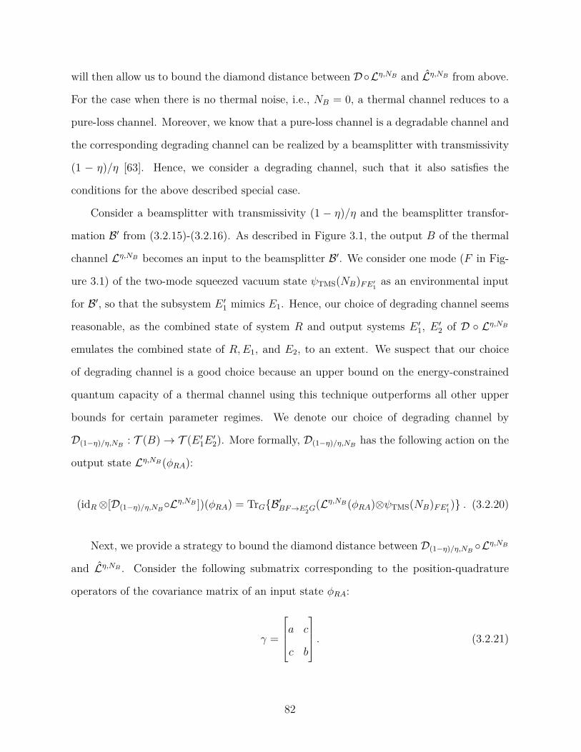
will then allow us to bound the diamond distance between D Lη ,NB and Lη ,NB from above.

For the case when there is no thermal noise, i.e., NB

= 0 , a thermal channel reduces to a

pure-loss channel. Moreover, we know that a pure-loss channel is a degradable channel and

the corresponding degrading channel can be realized by a beamsplitter with transmissivity

(1 − η ) /η [63]. Hence, we consider a degrading channel, such that it also satisfies the

conditions for the above described special case.

Consider a beamsplitter with transmissivity (1 − η ) /η and the beamsplitter transfor-

mation B

′ from (3.2.15)-(3.2.16). As described in Figure 3.1, the output B of the thermal

channel Lη ,NB becomes an input to the beamsplitter B

′. We consider one mode ( F in Fig-

ure 3.1) of the two-mode squeezed vacuum state ψTMS( NB)F E

′

1

as an environmental input

for B

′, so that the subsystem E

′

1

mimics E1. Hence, our choice of degrading channel seems

reasonable, as the combined state of system R and output systems E

′

1, E

′

2

of D Lη ,NB

emulates the combined state of R , E1, and E2, to an extent. We suspect that our choice

of degrading channel is a good choice because an upper bound on the energy-constrained

quantum capacity of a thermal channel using this technique outperforms all other upper

bounds for certain parameter regimes. We denote our choice of degrading channel by

D(1 − η ) /η ,NB

: T ( B ) → T ( E

′

1

E

′

2) . More formally, D(1 − η ) /η ,NB

has the following action on the

output state Lη ,NB ( ϕR A) :

(idR

⊗ [ D(1 − η ) /η ,NB

Lη ,NB ])( ϕR A) = TrG

B

′

B F → E

′

2

G( Lη ,NB ( ϕR A) ⊗ ψTMS( NB)F E

′

1) .

(3.2.20)

Next, we provide a strategy to bound the diamond distance between D(1 − η ) /η ,NB

Lη ,NB

and Lη ,NB . Consider the following submatrix corresponding to the position-quadrature

operators of the covariance matrix of an input state ϕR A:

γ =

a c

c b

.

(3.2.21)

82

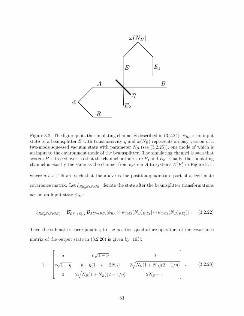
Figure 3.2: The figure plots the simulating channel Ξ described in (3.2.24). ϕR A

is an input

state to a beamsplitter B with transmissivity η and ω ( NB) represents a noisy version of a

two-mode squeezed vacuum state with parameter NB

(see (3.2.25)), one mode of which is

an input to the environment mode of the beamsplitter. The simulating channel is such that

system B is traced over, so that the channel outputs are E1

and E2. Finally, the simulating

channel is exactly the same as the channel from system A to systems E

′

1

E

′

2

in Figure 3.1.

where a, b, c ∈ R are such that the above is the position-quadrature part of a legitimate

covariance matrix. Let ξR E

′

2

E2

E1

GE

′

1

denote the state after the beamsplitter transformations

act on an input state ϕR A:

ξR E

′

2

E2

E1

GE

′

1

= B

′

B F → E

′

2

G[ BAE

′ → B E2 [ ϕR A

⊗ ψTMS( NB)E

′ E1 ] ⊗ ψTMS( NB)F E

′

1)] .

(3.2.22)

Then the submatrix corresponding to the position-quadrature operators of the covariance

matrix of the output state in (3.2.20) is given by [163]:

γ

′ =

a c√

1 − η 0

c√

1 − η b + η (1 − b + 2 NB) 2

√

NB(1 + NB)(2 − 1 /η )

0 2

√

NB(1 + NB)(2 − 1 /η ) 2 NB

+ 1

.

(3.2.23)

83

Now, we introduce a particular channel that simulates the action of D(1 − η ) /η ,NB

Lη ,NB

on an input state ϕR A. We denote this channel by Ξ , and it has the following action on an

input state ϕR A:

(idR

⊗ Ξ)( ϕR A) = Tr B

BAE

′ → B E2( ϕR A

⊗ ω ( NB)E

′ E1) ,

(3.2.24)

where ω ( NB)E

′ E1

represents a noisy version of a two-mode squeezed vacuum state with

parameter NB

and has the following submatrix corresponding to the position-quadrature

operators of the covariance matrix:

V

′ =

2 NB

+ 1 2

√

[ NB(1 + NB)(2 η − 1)] /η2

2

√

[ NB(1 + NB)(2 η − 1)] /η2 2 NB

+ 1

.

(3.2.25)

The matrix V

′ in (3.2.25) is a well defined submatrix of the covariance matrix for the noisy

version of a two-mode squeezed vacuum state, because (2 η − 1) /η2 ∈ [0 , 1] for η ∈ [1 / 2 , 1] .

The submatrix of the covariance matrix corresponding to the state in (3.2.24) is the same

as the submatrix in (3.2.23) [163]. In other words, the covariance matrix for the sytems

R , E

′

1, and E

′

2

in Figure 3.1 is exactly the same as the covariance matrix for the systems

R , E1, and E2

in Figure 3.2. This equality of covariance matrices is sufficient to conclude

that the following equivalence holds for an quantum input state ϕR A

(see [68, Chapter 5]

for a proof):

(idR

⊗ [ D(1 − η ) /η ,NB

Lη ,NB ])( ϕR A) = (idR

⊗ Ξ)( ϕR A) .

(3.2.26)

Thus, the channels D(1 − η ) /η ,NB

Lη ,NB and Ξ are indeed the same.

From (3.2.19), (3.2.24), and (3.2.26), the action of both Lη ,NB and Ξ can be understood

as tensoring the state of the environment with the input state of the channel, performing

the beamsplitter transformation B , and then tracing out the output of the channels. Using

these techniques, we now establish an upper bound on the diamond distance between the

complementary channel in (3.2.19) and the concatenation of the thermal channel followed

84

by the degrading channel in (3.2.20).

Theorem 76 Fix η ∈ [1 / 2 , 1] . Let Lη ,NB be a thermal channel with transmissivity η , and

let D(1 − η ) /η ,NB

be a degrading channel as defined in (3.2.20) . Then

1

2

∥∥∥ Lη ,NB − D(1 − η ) /η ,NB

Lη ,NB

∥∥∥⋄

≤

√

1 − η2 /κ ( η , NB) ,

(3.2.27)

with

κ ( η , NB) = η2 + NB( NB

+ 1)[1 + 3 η2 − 2 η (1 +

√

2 η − 1)] .

(3.2.28)

Proof. Consider the following chain of inequalities:

∥∥∥ (idR

⊗ Lη ,NB )( ϕR A) − (idR

⊗ [ D(1 − η ) /η ,NB

Lη ,NB ])( ϕR A)

∥∥∥1

=

∥∥∥ (idR

⊗ Lη ,NB )( ϕR A) − (idR

⊗ Ξ)( ϕR A)

∥∥∥1

(3.2.29)

= ∥ TrB

BAE

′ → B E2( ϕR A

⊗ ψTMS( NB)E

′ E1) − BAE

′ → B E2( ϕR A

⊗ ω ( NB)E

′ E1) ∥1

(3.2.30)

≤ ∥BAE

′ → B E2( ϕR A

⊗ ψTMS( NB)E

′ E1) − BAE

′ → B E2( ϕR A

⊗ ω ( NB)E

′ E1) ∥1

(3.2.31)

= ∥ ϕR A

⊗ ψTMS( NB)E

′ E1

− ϕR A

⊗ ω ( NB)E

′ E1

∥1

(3.2.32)

= ∥ ψTMS( NB)E

′ E1

− ω ( NB)E

′ E1

∥1

(3.2.33)

≤ 2

√

1 − F ( ψTMS( NB)E

′ E1

, ω ( NB)E

′ E1) (3.2.34)

The first equality follows from (3.2.26). The second equality follows from (3.2.19) and

(3.2.24). The first inequality follows from monotonicity of the trace distance. The third

equality follows from invariance of the trace distance under a unitary transformation (beam-

splitter). The last inequality follows from the Powers-Stormer inequality [135].

Next, we compute the fidelity between ψTMS( NB)E

′ E1

and ω ( NB)E

′ E1

by using their

respective covariance matrices in (3.2.18) and (3.2.25), in the Uhlmann fidelity formula for

85

two-mode Gaussian states [166]. We find [163]

F ( ψTMS( NB)E

′ E1

, ω ( NB)E

′ E1) =

η2

η2 + NB( NB

+ 1)[1 + 3 η2 − 2 η (1 +

√

2 η − 1)]

.

(3.2.35)

Since these inequalities hold for any input state ϕR A, the final result follows from the

definition of the diamond norm.


transmissivity η ∈ [1 / 2 , 1] , environment photon number NB, and input mean photon-number

constraint NS

is given by

Q ( Lη ,NB , NS) ≤ QU2( Lη ,NB , NS) ≡ g ( η NS

+ (1 − η ) NB) − g ( ζ+) − g ( ζ−)

+ (2 ε′ + 4 δ ) g ([(1 − η ) NS

+ (1 + η ) NB] /δ ) + g ( ε′) + 2 h2( δ ) , (3.2.36)

with

ε =

√

1 − η2 /

(

η2 + NB( NB

+ 1)[1 + 3 η2 − 2 η (1 +

√

2 η − 1)]

)

, (3.2.37)

ζ±

=

1

2

(

− 1 +

√

[(1 + 2 NB)2 − 2 ϱ + (1 + 2 ϑ )2 ± 4( ϑ − NB)

√

[1 + NB

+ ϑ ]2 − ϱ ] / 2

)

,

(3.2.38)

ϱ = 4 NB( NB

+ 1)(2 η − 1) /η , (3.2.39)

ϑ = η NB

+ (1 − η ) NS

, (3.2.40)

ε′ ∈ ( ε, 1] , and δ = ( ε′ − ε ) / (1 + ε′) .

Proof. From Theorem 76, we have an upper bound on the diamond distance between

the complementary channel of the thermal channel and the concatenation of the thermal

86

channel followed by the degrading channel, i.e.,

1

2

∥∥∥ Lη ,NB − D(1 − η ) /η ,NB

Lη ,NB

∥∥∥⋄

≤

√

1 − η2 /

(

η2 + NB( NB

+ 1)[1 + 3 η2 − 2 η (1 +

√

2 η − 1)]

)

< ε′ ≤ 1 . (3.2.41)

Due to the input mean photon number constraint NS, and environment photon number NB

for both Lη ,NB and D(1 − η ) /η ,NB, there is a total photon number constraint (1 − η ) NS

+ (1 +

η ) NB

for the average output of n channel uses of both Lη ,NB and D(1 − η ) /η ,NB

Lη ,NB . Using

these results in Theorem 68, we find the following upper bound on the energy-constrained

quantum capacity of a thermal channel:

Q ( Lη ,NB , NS) ≤ UD(1 − η ) /η ,NB( Lη ,NB , NS)+(2 ε′+4 δ ) g ([(1 − η ) NS+(1+ η ) NB] /δ )+ g ( ε′)+2 h2( δ ) .

(3.2.42)

Using Proposition 78, we find that the thermal state with mean photon number NS

opti-

mizes the conditional entropy of degradation UD(1 − η ) /η ,NB( Lη ,NB , NS) . For the given thermal

channel in (3.2.17) and the degrading channel in (3.2.20), we find the following analytical

expression [163]:

UD(1 − η ) /η ,NB( Lη ,NB , NS) = g ( η NS

+ (1 − η ) NB) − g ( ζ+) − g ( ζ−) ,

(3.2.43)

with ζ±

defined as in the theorem statement.

Proposition 78 Let Lη ,NB be a thermal channel with transmissivity η ∈ [1 / 2 , 1] , environ-

ment photon number NB, and input mean photon number constraint NS. Let D(1 − η ) /η ,NB

be the degrading channel from (3.2.20) . Then the thermal state with mean photon number

NS

optimizes the conditional entropy of degradation UD(1 − η ) /η ,NB( Lη ,NB , NS) , defined from

(3.1.2) .

Proof. Consider the Stinespring dilation in (3.2.22) of the degrading channel D(1 − η ) /η ,NB

87

from (3.2.20), and denote it by W . Then according to (3.1.2),

UD(1 − η ) /η ,NB( Lη ,NB , NS) = sup

ρ : Tr ˆ nρ ≤ NS

H ( G | E

′

1

E

′

2)( W Lη ,NB )( ρ )

.

(3.2.44)

Our aim is to find an input state ρ with a certain photon number Nt

≤ NS, such that it

maximizes the conditional entropy in (3.2.44). From the extremality of Gaussian states

applied to the conditional entropy [167], it suffices to perform the optimization in (3.2.44)

over only Gaussian states.

Now, we argue that for a given input mean photon number Nt, a thermal state is the

optimal state for the conditional output entropy in (3.2.44). For a thermal channel and

our choice of a degrading channel, a phase rotation on the input state is equivalent to a

product of local phase rotations on the outputs. Let us denote the state after the local

phase rotations on the outputs by

σE

′

2

GE

′

1( ϕ ) = ( eiϕ ˆ n ⊗ eiϕ ˆ n ⊗ e− iϕ ˆ n)( W Lη ,NB )( ρ )( e− iϕ ˆ n ⊗ e− iϕ ˆ n ⊗ eiϕ ˆ n) ,

(3.2.45)

and let

ξE

′

2

GE

′

1

=

1

2 π

∫ 2 π

0

dϕ ( W Lη ,NB )( eiϕ ˆ n ρe− iϕ ˆ n) .

(3.2.46)

Note that the phase covariance property mentioned above is the statement that the follow-

ing equality holds for all ϕ ∈ [0 , 2 π ) [163]:

σE

′

2

GE

′

1( ϕ ) = ( W Lη ,NB )( eiϕ ˆ n ρe− iϕ ˆ n) .

(3.2.47)

88

Consider the following chain of inequalities for a Gaussian input state ρ :

H ( G | E

′

1

E

′

2)( W Lη ,NB )( ρ )

=

1

2 π

∫ 2 π

0

dϕ H ( G | E

′

1

E

′

2)σ ( ϕ )

(3.2.48)

=

1

2 π

∫ 2 π

0

dϕ H ( G | E

′

1

E

′

2)( W Lη ,NB )( eiϕ ˆ n ρe− iϕ ˆ n)

(3.2.49)

≤ H ( G | E

′

1

E

′

2)ξ

(3.2.50)

= H ( G | E

′

1

E

′

2)( W Lη ,NB )( θ ( Nt))

, (3.2.51)

The first equality follows from invariance of the conditional entropy under local unitaries.

The second equality follows from the phase covariance property of the channel. The inequal-

ity follows from concavity of conditional entropy. The last equality follows from linearity

of the channel, and the following identity:

θ ( Nt) =

1

2 π

∫ 2 π

0

dϕ eiϕ ˆ n ρe− iϕ ˆ n .

(3.2.52)

In (3.2.52), the state after the phase averaging is diagonal in the number basis, and fur-

thermore, the resulting state has the same photon number Nt

as the Gaussian state ρ . The

thermal state θ ( Nt) is the only Gaussian state of a single mode that is diagonal in the

number basis with photon number equal to Nt.

Next, we argue that, for a given photon number constraint, a thermal state that satu-

rates the constraint is the optimal state for the conditional output entropy. Let

τE

′

2

GE

′

1( α ) =

[ D (√

1 − η α ) ⊗ D (√

2 η − 1 α ) ⊗ I ][( W Lη ,NB )( θ ( Nt))][ D

†(√

1 − η α ) ⊗ D

†(√

2 η − 1 α ) ⊗ I ] .

(3.2.53)

89


H ( G | E

′

1

E

′

2)( W Lη ,NB )( θ ( Nt))

=

∫

d2 α q( NS

− Nt)( α ) H ( G | E

′

1

E

′

2)( W Lη ,NB )( θ ( Nt))

(3.2.54)

=

∫

d2 α q( NS

− Nt)( α ) H ( G | E

′

1

E

′

2)τ ( α )

(3.2.55)

=

∫

d2 α q( NS

− Nt)( α ) H ( G | E

′

1

E

′

2)( W Lη ,NB )( D ( α ) θ ( Nt) D

†( α ))

(3.2.56)

≤ H ( G | E

′

1

E

′

2)( W Lη ,NB ) θ ( NS)

, (3.2.57)

where qN( α ) = exp −| α |2 /N /π N is a complex-centered Gaussian distribution with vari-

ance N ≥ 0 . The first equality follows by placing a probability distribution in front, and

the second follows from invariance of the conditional entropy under local unitaries. The

third equality follows because the channel is covariant with respect to displacement op-

erators, as reviewed in (2.3.69). The last inequality follows from concavity of conditional

entropy, and from the fact that a thermal state with a higher mean photon number can be

realized by random Gaussian displacements of a thermal state with a lower mean photon

number, as reviewed in (2.3.33). Hence, for a given input mean photon number constraint

NS, a thermal state with mean photon number NS

optimizes the conditional entropy of

degradation defined from (3.1.2).

Remark 79 The arguments used in the proof of Proposition 78 can be employed in more

general situations beyond that which is discussed there. The main properties that we need

are the following, when the channel involved takes a single-mode input to a multi-mode

output:

• The channel should be phase covariant, such that a phase rotation on the input state

is equivalent to a product of local phase rotations on the output.

• The channel should be covariant with respect to displacement operators, such that

a displacement operator acting on the input state is equivalent to a product of local

90

displacement operators on the output.

• The function being optimized should be invariant with respect to local unitaries and

concave in the input state.

If all of the above hold, then we can conclude that the thermal-state input saturating the

energy constraint is an optimal input state. We employ this reasoning again in the proof of

Theorem 87. It has also been used in [151].

3.2.3 ε -Close-Degradable Bound on the Energy-Constrained Quantum Ca-

pacity of Bosonic Thermal Channels

In this section, we first establish an upper bound on the diamond distance between a

thermal channel and a pure-loss channel. Since a pure-loss channel is a degradable channel,

an upper bound on the energy-constrained quantum capacity of a thermal channel directly

follows from Theorem 69.

Theorem 80 If a thermal channel Lη ,NB and a pure-loss bosonic channel Lη , 0 have the

same transmissivity parameter η ∈ [0 , 1] , then

1

2

∥∥∥ Lη ,NB − Lη , 0

∥∥∥⋄

≤

NB

NB

+ 1

.

(3.2.58)

Proof. Let B represent the beamsplitter transformation, and let θE( NB) and θ

′

E(0) denote

the states of the environment for the thermal channel and pure-loss channel, respectively.

For every input state ψR A

to both thermal and pure-loss channels, the following inequalities

91

hold:

∥∥∥ (idR

⊗Lη ,NB )( ψR A) − (idR

⊗Lη , 0)( ψR A)

∥∥∥1

= ∥ TrE

′ BAE → B E

′( ψR A

⊗ θE( NB)) − BAE → B E

′( ψR A

⊗ θ

′

E(0)) ∥1

(3.2.59)

≤ ∥BAE → B E

′( ψR A

⊗ θE( NB)) − BAE → B E

′( ψR A

⊗ θ

′

E(0)) ∥1

(3.2.60)

= ∥ ψR A

⊗ θE( NB) − ψR A

⊗ θ

′

E(0) ∥1

(3.2.61)

= ∥ θE( NB) − θ

′

E(0) ∥1

(3.2.62)

=

∥∥∥∥∥

∞∑

n =0

( NB)n

( NB

+ 1)n +1

| n ⟩⟨ n | − | 0 ⟩⟨ 0 |

∥∥∥∥∥

1

(3.2.63)

=

2 NB

NB

+ 1

. (3.2.64)

The first equality follows from the definition of the channel in terms of its environment and

a unitary interaction (beam splitter). The first inequality follows from monotonicity of the

trace distance. The second equality follows from invariance of the trace distance under a

unitary operator (beamsplitter). The last equality follows from basic algebra. Since these

inequalities hold for every state ψR A, the final result follows from the definition of the

diamond norm.

Remark 81 In [168], it has been shown that the optimal strategy to distinguish two quan-

tum thermal channels Lη ,N1

B and Lη ,N2

B , each having the same transmissivity parameter η ,

and thermal noises N1

B

and N2

B, respectively, is to use a highly squeezed, two-mode squeezed

vacuum state ψTMS( NS)R A

as input to the channels. According to [168, Eq. (35)],

lim

NS

→∞

F ( σN1

B

, σN2

B) = F ( θ ( N1

B) , θ ( N2

B)) ,

(3.2.65)

where σN

i

B

≡ (idR

⊗Lη ,N

i

B )( ψTMS( NS)R A) , and θ ( N

i

B) is a thermal state with mean photon

92

number N

i

B. Hence, a lower bound on the diamond distance in Theorem 80 is given by

1

2

∥∥∥ Lη ,NB − Lη , 0

∥∥∥⋄

≥ 1 −

√

F ( θ ( NB) , θ (0)) = 1 − 1 /

√

NB

+ 1 ,

(3.2.66)

where the inequality follows from the Powers-Stormer inequality [135]. We also suspect

that the upper bound in Theorem 80 is achievable, but we are not aware of a method for

computing the trace distance of general quantum Gaussian states, which is what it seems

would be needed to verify this suspicion.


transmissivity η ∈ [1 / 2 , 1] , environment photon number NB, and input mean photon number

constraint NS

is given by

Q ( Lη ,NB , NS) ≤ QU3( Lη ,NB , NS) ≡ g ( η NS) − g [(1 − η ) NS]

+ (4 ε′ + 8 δ ) g [( η NS

+ (1 − η ) NB) /δ ] + 2 g ( ε′) + 4 h2( δ ) , (3.2.67)

with ε = NB

/ ( NB

+ 1) , ε′ ∈ ( ε, 1] and δ = ( ε′ − ε ) / (1 + ε′) .

Proof. From Theorem 80, we have that

1

2

∥∥∥ Lη ,NB − Lη , 0

∥∥∥⋄

≤

NB

NB+1

< ε′ ≤ 1 . Due to the

input mean photon number constraint NS

for n channel uses, the output mean photon

number cannot exceed η NS

+ (1 − η ) NB

for the thermal channel and η NS

for the pure-loss

channel. Hence, there is a photon number constraint η NS

+ (1 − η ) NB

for the output

of both the thermal and pure-loss channels. Since the pure-loss channel is a degradable

channel for η ∈ [1 / 2 , 1] [63, 160], the final result follows directly from Theorem 69.

3.2.4 Bottleneck Bound on the Energy-Constrained Quantum Capacity of


In this section we establish an upper bound on the quantum capacity of a thermal chan-

nel using Theorem 83 below, which states that any phase-insensitive single-mode bosonic

93

Gaussian channel can be decomposed as a pure-amplifier channel followed by a pure-loss

channel, if the original channel is not entanglement breaking. This theorem was indepen-

dently proven in [148,149] (see also [150] in this context).

Before we state the theorem, let us recall that the action of a phase-insensitive channel

N on the covariance matrix Γ of a single-mode, bosonic quantum state is given by

Γ 7−→ τ Γ + ν I2

, (3.2.68)

where ν is the variance of an additive noise, I2

is the 2 × 2 identity matrix, and τ and

ν satisfy the conditions in (2.3.74)–(2.3.75). Moreover, as mentioned previously, a phase-

insensitive channel N is entanglement-breaking [125,126] if

τ + 1 ≤ ν .

(3.2.69)

Theorem 83 Any single-mode, phase-insensitive bosonic Gaussian channel N that is not

entanglement-breaking (i.e., satisfies τ + 1 > ν ) can be decomposed as the concatenation of

a quantum-limited amplifier channel AG, 0 with gain G > 1 followed by a pure-loss channel

Lη , 0 with transmissivity η ∈ (0 , 1] , i.e.,

N = Lη , 0 AG, 0 ,

(3.2.70)

where η = ( τ + 1 − ν ) / 2 and G = τ /η .

Proof. The action of a quantum-limited amplifier channel AG, 0 with gain G followed by a

pure-loss channel Lη , 0 with transmissivity η , on convariance matrix Γ is given by

η ( G Γ + [ G − 1] I2) + [1 − η ] I2

.

(3.2.71)

By comparing (3.2.68) and (3.2.71), we find that it is necessary for the following equalities

94

to hold

η G = τ , (3.2.72)

η ( G − 1) + 1 − η = ν . (3.2.73)

Solving these equations for η and G in terms of τ and ν then gives η = ( τ + 1 − ν ) / 2 and

G = τ /η . By the assumption that N is not entanglement breaking, which is that τ +1 > ν ,

we find that

η = ( τ + 1 − ν ) / 2 > 0 .

(3.2.74)

Now applying the conditions in (2.3.74) and (2.3.75) for the channel N to be a CPTP map,

we find that

η = ( τ + 1 − ν ) / 2 ≤ ( τ + 1 − | 1 − τ | ) / 2 =

τ for τ ∈ [0 , 1)

1 for τ ≥ 1

(3.2.75)

By the fact that G = τ /η , the above implies that G > 1 , so that the decomposition in

(3.2.70) is valid under the stated conditions.

We now introduce an upper bound on the energy-constrained quantum capacity of

thermal channels in the following theorem (independently discovered in [149] as well):

Theorem 84 An upper bound on the energy-constrained quantum capacity of a thermal

channel Lη ,NB with transmissivity η ∈ [1 / 2 , 1] , environment photon number NB

≥ 0 , such

that η > (1 − η ) NB, and input mean photon number constraint NS

≥ 0 is given by

Q ( Lη ,NB , NS) ≤ max 0 , QU4( Lη ,NB , NS) ,

(3.2.76)

where

QU4( Lη ,NB , NS) ≡ g ( η NS

+ (1 − η ) NB) − g [(1 /η

′ − 1)( η NS

+ (1 − η ) NB)] ,

(3.2.77)

95

and η

′ = η − (1 − η ) NB.

Proof. Using Theorem 83, a thermal channel Lη ,NB satisfying η > (1 − η ) NB

can be

decomposed as the concatenation of a quantum-limited amplifier channel AG, 0 followed by

a pure-loss channel Lη

′ , 0, such that

G = η /η

′ , (3.2.78)

η

′ = η − (1 − η ) NB

. (3.2.79)


Q ( Lη ,NB , NS) = Q ( Lη

′ , 0 AG, 0 , NS) (3.2.80)

≤ Q ( Lη

′ , 0 , GNS

+ G − 1) (3.2.81)

= g ( η

′[ GNS

+ G − 1]) − g [(1 − η

′)( GNS

+ G − 1)] (3.2.82)

= g ( η NS

+ (1 − η ) NB) − g [(1 /η

′ − 1)( η NS

+ (1 − η ) NB)] . (3.2.83)

The first inequality is a consequence of the following argument: consider an arbitrary

encoding and decoding scheme for energy-constrained quantum communication over the

thermal channel Lη ,NB , which satisfies the mean input photon number constraint NS

≥ 0 .

Due to the decomposition of Lη ,NB as Lη

′ , 0 AG, 0, this encoding, followed by many uses of the

pure-amplifier channel AG, 0 can be considered as an encoding for the channel Lη

′ , 0, which

also satisfies the mean photon number constraint GNS+ G − 1 , due to the fact that the pure-

amplifier channel AG, 0 introduces a gain. Since the energy-constrained quantum capacity

of the channel Lη

′ , 0 involves an optimization over all such encodings that satisfies the mean

photon number constraint GNS

+ G − 1 , we arrive at the desired inequality. The second

equality follows from the formula for the energy-constrained quantum capacity of a pure-loss

bosonic channel with transmissivity η

′ and input mean photon number GNS+ G − 1 [62,64].

96

Remark 85 Applying Remark 65, we find the following bottleneck bound QU4( Lη ,NB ) on

the unconstrained quantum capacity of bosonic thermal channels for which η > (1 − η ) NB:

Q ( Lη ,NB ) ≤ QU4( Lη ,NB ) = sup

NS : NS

∈ [0 , ∞ ]

QU4( Lη ,NB , NS) (3.2.84)

= lim

NS

→∞

QU4( Lη ,NB , NS) (3.2.85)

= max

0 , log2

(

η − (1 − η ) NB

(1 − η )( NB

+ 1)

)

. (3.2.86)

The aforementioned bound on the unconstrained quantum capacity of a thermal channel

was also established independently in [148]. Note that (3.2.86) is slightly tighter than

(3.2.9) for all parameter regimes. These findings were independently discovered in [149].

Remark 86 The upper bound QU4( Lη ,NB , NS) on the energy-constrained quantum and pri-

vate capacities of thermal channels places a strong restriction on the channel parameters

η and NB. Since the quantum and private capacities of a pure-loss channel with η

′ are

non-zero only for η

′ > 1 / 2 , the energy-constrained quantum and private capacities of a

thermal channel will be non-zero only for

1 ≥ η >

1 + 2 NB

2(1 + NB)

,

(3.2.87)

which is the same as the condition given in [127, Section 4].

3.3 Comparison of Upper Bounds on the Energy-Constrained Quantum Ca-

pacity of Bosonic Thermal Channels

In this section, we study the closeness of the four different upper bounds when compared

to a known lower bound. In particular, we use the following lower bound on the quantum

97

capacity of a thermal channel [64, 147] and denote it by QL:

Q ( Lη ,NB , NS) ≥ QL( Lη ,NB , NS) ≡ g ( η NS

+ (1 − η ) NB)

− g ([ D + (1 − η ) NS

− (1 − η ) NB

− 1] / 2) − g ([ D − (1 − η ) NS

+ (1 − η ) NB

− 1] / 2) ,

(3.3.1)

where

D2 ≡ [(1 + η ) NS

+ (1 − η ) NB

+ 1]2 − 4 η NS( NS

+ 1) .

(3.3.2)

We start by discussing how close the data-processing bound QU1

is to the aforementioned

lower bound. In particular, we show that the data-processing bound QU1

can be at most

1 . 45 bits larger than QL.

Theorem 87 Let Lη ,NB be a thermal channel with transmissivity η ∈ [1 / 2 , 1] , environment

photon number NB, and input mean photon number constraint NS. Then the following

relation holds between the data-processing bound QU1( Lη ,NB , NS) in (3.2.3) and the lower

bound QL( Lη ,NB , NS) in (3.3.1) on the energy-constrained quantum capacity of a thermal

channel:

QL( Lη ,NB , NS) ≤ QU1( Lη ,NB , NS) ≤ QL( Lη ,NB , NS) + 1 / ln 2 .

(3.3.3)

Proof. To prove this result, we first compute the difference between the data-processing

bound in (3.2.3) and the lower bound in (3.3.1) and show that it is equal to 1 / ln 2 as NS

→

∞ . Next, we prove that the difference is a monotone increasing function with respect to

input mean photon number NS

≥ 0 . Hence, the difference QU1( Lη ,NB , NS) − QL( Lη ,NB , NS)

attains its maximum value in the limit NS

→ ∞ . We note that a similar statement has

been given in [144] to bound the classical capacity of a thermal channel, but the details of

the approach we develop here are different and are likely to be more broadly applicable to

related future questions.

For simplicity, we denote (1 − η ) NB

as Y , employ the natural logarithm for g ( x ) , and

98

omit the prefactor 1 / ln 2 from all instances of g ( x ) . We use the following property of the

function g ( x ) : For large x ,

g ( x ) = ln( x + 1) + 1 + O (1 /x ) ,

(3.3.4)

so that as x → ∞ , the approximation g ( x ) ≈ ln( x + 1) + 1 holds. Using (3.3.4), the

data-processing bound in (3.2.3) can be expressed as follows for large NS:

ln( Y + 1 + η NS) − ln( Y + 1 + ( Y + 1 − η ) NS) + O (1 /NS) .

(3.3.5)

Similarly, the lower bound QL

in (3.3.1) can be expressed as

ln(1 + η NS

+ Y ) − ln([1 + D + (1 − η ) NS

− Y ] / 2) − ln([1 + D − (1 − η ) NS

+ Y ] / 2)

+ O (1 /NS) − 1 . (3.3.6)

Let us denote the difference between QU1

and QL

by ∆( Lη ,NB , NS) .

∆( Lη ,NB , NS) = QU1( Lη ,NB , NS) − QL( Lη ,NB , NS) .

(3.3.7)

Then the difference simplifies as

∆( Lη ,NB , NS)

= 1 − ln( Y + 1 + ( Y + 1 − η ) NS) + ln

(

[(1 + D )2 − ((1 − η ) NS

− Y )2] / 4

)

+ O (1 /NS) .

(3.3.8)

= 1 − ln( Y + 1 + ( Y + 1 − η ) NS) + ln([1 + NS(1 − η + 2 Y ) + Y + D ] / 2) + O (1 /NS)

(3.3.9)

= 1 + ln([1 + NS(1 − η + 2 Y ) + Y + D ] / [2( Y + 1 + ( Y + 1 − η ) NS)]) + O (1 /NS) .

(3.3.10)

99

The second equality follows from the definition of D2. Next, we show that

ln([1 + NS(1 − η + 2 Y ) + Y + D ] / [2( Y + 1 + ( Y + 1 − η ) NS)]) → 0

(3.3.11)

as NS

→ ∞ , and hence we get the desired result. Consider the following expression and

take the limit NS

→ ∞ :

lim

NS

→∞

1 + NS(1 − η + 2 Y ) + Y + D

2( Y + 1 + ( Y + 1 − η ) NS)

(3.3.12)

= lim

NS

→∞

1 /NS

+ (1 − η + 2 Y ) + Y /NS

+

√

((1 + η ) + ( Y + 1) /NS)2 − 4 η − 4 η /NS

2(( Y + 1) /NS

+ ( Y + 1 − η ))

(3.3.13)

→

(1 − η + 2 Y ) + 1 − η

2( Y + 1 − η )

= 1 . (3.3.14)

Hence, lim NS

→∞ ∆( Lη ,NB , NS) = 1 . After incorporating the 1 / ln 2 factor, which was omit-

ted earlier for simplicity, we find that the difference between the upper and lower bounds

approaches 1 / ln 2 ( ≈ 1.45 bits) as NS

→ ∞ .

Now, we show that the difference ∆( Lη ,NB , NS) is a monotone increasing function with

respect to the input mean photon number NS

≥ 0 . Let U

η

′

A → B1

E1

and V

G

B1

→ B2

E2

denote

Stinespring dilations of a pure-loss channel Lη

′ , 0 : A → B1

and a quantum limited amplifier

channel AG, 0 : B1

→ B2, respectively. For the energy-constrained quantum capacity of a

pure-loss channel, the thermal state as an input is optimal for any fixed energy or input

mean photon number constraint NS

[64]. Moreover, the lower bound in (3.3.1) is obtained

for a thermal state with mean photon number NS

as input to the channel. Then the action

of a thermal channel Lη ,NB on an input state θ ( NS) can be expressed as

Lη ,NB ( θ ( NS)) = TrE1

E2

(idE1

⊗V

G

B1

→ B2

E2) U

η

′

A → B1

E1( θ ( NS)) .

(3.3.15)

100

Consider the following state:

ωB2

E1

E2

= (idE1

⊗V

G

B1

→ B2

E2) U

η

′

A → B1

E1( θ ( NS)) . (3.3.16)

Since the data-processing bound QU1( Lη ,NB , NS) is equal to the quantum capacity of a

pure-loss channel with transmissivity η

′, which in turn is equal to the coherent information

for this case, (3.2.3) can also be represented as

QU1( Lη ,NB , NS) = H ( B2

E2)ω

− H ( E1)ω

. (3.3.17)

Similarly, the lower bound can be expressed as

QL( Lη ,NB , NS) = H ( B2)ω

− H ( E1

E2)ω

. (3.3.18)

Hence the difference between (3.3.17) and (3.3.18) is given by

∆( Lη ,NB , NS) = H ( E2

| B2)ω

+ H ( E2

| E1)ω

. (3.3.19)

Now, our aim is to show that the conditional entropies in (3.3.19) are monotone increasing

functions of NS. We employ displacement covariance of the channels, and note that this

argument is similar to that used in the proof of Proposition 78. Let

σB2

E1

E2( α ) = [ D (

√

η Gα ) ⊗ I ⊗ D (

√

η ( G − 1) α )] ωB2

E1

E2

× [ D

†(

√

η Gα ) ⊗ I ⊗ D

†(

√

η ( G − 1) α )] , (3.3.20)

τB2

E1

E2( α ) = [ I ⊗ D (√

1 − η α ) ⊗ D (

√

η ( G − 1) α )] ωB2

E1

E2

× [ I ⊗ D

†(√

1 − η α ) ⊗ D

†(

√

η ( G − 1) α )] . (3.3.21)

101

Let N

′

S

− NS

≥ 0 , and consider the following chain of inequalities:

H ( E2

| B2)ω

+ H ( E2

| E1)ω

=

∫

d2 α q( N

′

S

− NS)( α ) [ H ( E2

| B2)ω

+ H ( E2

| E1)ω] (3.3.22)

=

∫

d2 α q( N

′

S

− NS)( α ) [ H ( E2

| B2)σ ( α )

+ H ( E2

| E1)τ ( α )] (3.3.23)

=

∫

d2 α q( N

′

S

− NS)( α ) [ H ( E2

| B2)( V

G U

η

′ )( D ( α ) θ ( NS) D

†( α ))]

+

∫

d2 α q( N

′

S

− NS)( α ) [ H ( E2

| E1)( V

G U

η

′ )( D ( α ) θ ( NS) D

†( α ))]

(3.3.24)

≤ H ( E2

| B2)( V

G U

η

′ )( θ ( N

′

S))

+ H ( E2

| E1)( V

G U

η

′ )( θ ( N

′

S))

. (3.3.25)

The first equality follows by placing a probability distribution in front, and the second

follows from invariance of the conditional entropy under local unitaries. The third equality

follows because the channel is covariant with respect to displacement operators, as reviewed

in (2.3.69). The last inequality follows from concavity of conditional entropy, and from the

fact that a thermal state with a higher mean photon number can be realized by random

Gaussian displacements of a thermal state with a lower mean photon number, as reviewed

in (2.3.33).

Hence, the difference between the data-processing bound in (3.2.3) and the lower bound

in (3.3.1) attains its maximum value in the limit NS

→ ∞ .

Next, we perform numerical evaluations to see how close the four different upper bounds

are to the lower bound QL

in (3.3.1). Since there is a free parameter ε′ in both the ε -

degradable bound in (3.2.36) and the ε -close-degradable bound in (3.2.67), we optimize

these bounds with respect to ε′ [163]. In Figure 3.3, we plot the data-processing bound

QU1 , the ε -degradable bound QU2 , the ε -close-degradable bound QU3 , the bottleneck bound

QU4 , and the lower bound QL

versus NS

for certain values of the transmissivity η and

thermal noise NB. In particular, we find that both the data-processing bound and the

bottleneck bound are close to the lower bound QL

for both low and high thermal noise. In

102

(a)

(b)

(c)

(d)

Figure 3.3: The figures plot the data-processing bound ( QU1) , the ε -degradable bound

( QU2) , the ε -close-degradable bound ( QU3) , the bottleneck bound QU4 , and the lower bound

( QL) on energy-constrained quantum capacity of thermal channels. In each figure, we select

certain values of η and NB, with the choices indicated above each figure. In all the cases,

both the data-processing bound QU1

and the bottleneck bound QU4

are close to the lower

bound QUL. In (a), for medium transmissivity and low thermal noise, the ε -close-degradable

bound is close to the data-processing bound and the bottleneck bound, and they are tighter

than the ε -degradable bound. In (b), for medium transmissivity and high thermal noise,

only the data-processing bound and the bottleneck bound are close to the lower bound.

Also the ε -degradable bound is tighter than the ε -close-degradable bound. In (c), for high

transmissivity and low thermal noise, all upper bounds are very near to the lower bound.

In (d), for high transmissivity and high noise, the ε -degradable bound is tighter than the

ε -close-degradable bound.

103

particular, for the data-processing bound QU1 , this is related to Theorem 87, as QU1

can

be at most 1.45 bits larger than the lower bound QL. In Figure 3.3(a), we plot for medium

transmissivity and low thermal noise. We find that the ε -close-degradable bound is very

near to the data-processing bound and is tighter than the ε -degradable bound. Moreover,

QU4

is slightly tighter than QU1

for some parameter regimes. In Figure 3.3(b), we plot for

medium transmissivity and high thermal noise. We find that the ε -degradable bound is

tighter than the ε -close degradable bound. In Figure 3.3(d), we plot for high transmissivity

and high thermal noise. In Figure 3.3(c), we plot for high transmissivity and low thermal

noise. We find that all upper bounds are very near to the lower bound QL. From Figures

3.3(a) and 3.3(c), it is evident that in the low-noise regime, there is a strong limitation on

any potential super-additivity of coherent information of a thermal channel. Similar results

were obtained on quantum and private capacities of low-noise quantum channels in [169].

It is important to stress that the upper bound QU3

can serve as a good bound only for

low values of the thermal noise NB, as the technique to calculate this bound requires the

closeness of a thermal channel with a pure-loss channel (discussed in Theorem 80), and the

closeness parameter is equal to NB

/ ( NB

+ 1) .

In Figure 3.4, we plot all the upper bounds and the lower bound QL

versus NS, for

high transmissivity and high thermal noise. In Figure 3.4(a), we find that the ε -degradable

bound is tighter than all other bounds for high values of NS. In Figure 3.4(b), we plot for

the same parameter values, but for low values of NS. It is evident that for low input mean

photon number, both the data-processing bound and the bottleneck bound are tighter than

the ε -degradable bound.

The plots suggest that our upper bounds based on the notion of approximate degrad-

ability are good for the case of high input mean photon number. We suspect that these

bounds can be further improved for the case of low input mean photon number by consider-

ing the energy-constrained diamond norm [137,138]. To address this question, we consider

the generalized channel divergences of quantum Gaussian channels in Section 3.8 and argue

104

about their optimization.

3.4 Upper Bounds on Energy-Constrained Private Capacity of Bosonic Ther-

mal Channels

In this section, we provide four different upper bounds on the energy-constrained pri-

vate capacity of a thermal channel. These upper bounds are derived very similarly as in

Section 3.2. We call these different bounds the data-processing bound, the ε -degradable

bound, the ε -close-degradable bound, and the bottleneck bound, and denote them by PU1 ,

PU2 , PU3 , and PU4 , respectively.

3.4.1 Data-Processing Bound on the Energy-Constrained Private Capacity

of Bosonic Thermal Channels

Theorem 88 An upper bound on the private capacity of a thermal channel Lη ,NB with

transmissivity η ∈ [1 / 2 , 1] , environment photon number NB

≥ 0 , and input mean photon

number constraint NS

≥ 0 is given by

P ( Lη ,NB , NS) ≤ max 0 , PU1( Lη ,NB , NS) (3.4.1)

PU1( Lη ,NB , NS) ≡ g ( η

′ NS) − g [(1 − η

′) NS] , (3.4.2)

with η

′ = η / ((1 − η ) NB

+ 1) .

Proof. A proof follows from arguments similar to those in the proof of Theorem 73. Since

a pure-loss channel is a degradable channel [63,160], its energy-constrained private capacity

is the same as its energy-constrained quantum capacity [62].

Remark 89 Applying Remarks 65 and 74, we find the following data-processing bound

PU1( Lη ,NB ) on the unconstrained private capacity P ( Lη ,NB ) of a thermal channel Lη ,NB :

P ( Lη ,NB ) ≤ PU1( Lη ,NB ) = log2( η / (1 − η )) − log2( NB

+ 1) . (3.4.3)

105

(a)

(b)

Figure 3.4: The figures plot the data-processing bound ( QU1) , the ε -degradable bound

( QU2) , and the lower bound ( QL) on energy-constrained quantum capacity of thermal

channels (the ε -close-degradable bound ( QU3) is not plotted because it is much higher than

the other bounds for all parameter values considered). In each figure, we select η = 0 . 99

and NB

= 0 . 5 . In (a), the ε -degradable upper bound is tighter than all other upper bounds.

In (b), for low values of NS, the data-processing bound is tighter than the ε -degradable

bound.

106

3.4.2 ε -Degradable Bound on the Energy-Constrained Private Capacity of






≥ 0 is given by

P ( Lη ,NB , NS) ≤ PU2( Lη ,NB , NS) ≡ g ( η NS

+ (1 − η ) NB) − g ( ζ+) − g ( ζ−)

+ (6 ε′ + 12 δ ) g ([(1 − η ) NS

+ (1 + η ) NB] /δ ) + 3 g ( ε′) + 6 h2( δ ) , (3.4.4)

with

ε =

√

1 − η2 /

(

η2 + NB( NB

+ 1)[1 + 3 η2 − 2 η (1 +

√

2 η − 1)]

)

, (3.4.5)

ζ±

=

1

2

(

− 1 +

√

[(1 + 2 NB)2 − 2 ϱ + (1 + 2 ϑ )2 ± 4( ϑ − NB)

√

[1 + NB

+ ϑ ]2 − ϱ ] / 2

)

,

(3.4.6)

ϱ = 4 NB( NB

+ 1)(2 − 1 /η ) , (3.4.7)

ϑ = η NB

+ (1 − η ) NS

, (3.4.8)

ε′ ∈ ( ε, 1] , and δ = ( ε′ − ε ) / (1 + ε′) .

Proof. A proof follows from arguments similar to those in the proof of Theorem 77. The

final result is obtained using Theorem 71.

3.4.3 ε -Close-Degradable Bound on the Energy-Constrained Private Capac-

ity of Bosonic Thermal Channels




107


≥ 0 is given by

P ( Lη ,NB , NS) ≤ PU3( Lη ,NB , NS) ≡ g ( η NS) − g [(1 − η ) NS]

+ (8 ε′ + 16 δ ) g [( η NS

+ (1 − η ) NB) /δ ] + 4 g ( ε′) + 8 h2( δ ) , (3.4.9)

with ε = NB

/ ( NB

+ 1) , ε′ ∈ ( ε, 1] , and δ = ( ε′ − ε ) / (1 + ε′) .



3.4.4 Bottleneck Bound on the Energy-Constrained Private Capacity of Bosonic

Thermal Channels



≥ 0 , such that η > (1 − η ) NB,

and input mean photon number constraint NS

≥ 0 is given by

P ( Lη ,NB , NS) ≤ max 0 , PU4( Lη ,NB , NS) (3.4.10)

PU4( Lη ,NB , NS) ≡ g ( η NS

+ (1 − η ) NB) − g [(1 /η

′ − 1)( η NS

+ (1 − η ) NB)] , (3.4.11)

and η

′ = η − (1 − η ) NB.

Proof. A proof follows from arguments similar to those in the proof of Theorem 84. Since

a pure-loss channel is a degradable channel [63,160], its energy-constrained private capacity

is the same as its energy-constrained quantum capacity [62].

3.5 Lower Bound on Energy-Constrained Private Capacity of Bosonic Ther-

mal Channels

In this section, we establish an improvement on the best known lower bound [64] on

the energy-constrained private capacity of bosonic thermal channels, by using displaced

thermal states as input to the channel. We note that a similar effect has been observed

in [170] for the finite-dimensional case.

108

The energy-constrained private information of a channel N , as defined in (2.7.11), can

also be written as

P (1)( N , G, W )

≡ sup

¯ ρEA:Tr G ¯ ρEA

≤ W[ H ( N (¯ ρEA

)) − H ( N (¯ ρEA)) −

∫

dx pX( x )[ H ( N ( ρx

A)) − H ( N ( ρx

A))]] ,

(3.5.1)

where ¯ ρEA

≡

∫

dx pX( x ) ρx

A

is an average state of the ensemble EA

≡ pX( x ) , ρx

A

and N de-

notes a complementary channel of N . If the energy-constrained private information is calcu-

lated for coherent-state inputs, then for each element of the ensemble, the following equality

holds H ( N ( ρx

A)) = H ( N ( ρx

A)) . Hence, the entropy difference H ( N (¯ ρEA)) − H ( N (¯ ρEA

)) is

an achievable rate, which is the same as the energy-constrained coherent information.

However, we show that displaced thermal-state inputs provide an improved lower bound

for certain values of the transmissivity η , low thermal noise NB, and both low and high

input mean photon number NS. We start with the following ensemble of displaced thermal

states,

E ≡ pN1

S( α ) , D ( α ) θ ( N2

S) D ( − α ) ,

(3.5.2)

chosen according to the Gaussian probability distribution

pN1

S( α ) =

1

π N1

S

exp

(

−| α |2 /N1

S

)

,

(3.5.3)

where D ( α ) denotes the displacement operator, θ ( N2

S) denotes the thermal state with mean

photon number N2

S, and N1

S

and N2

S

are chosen such that N1

S

+ N2

S

= NS, which is the

mean number of photons input to the channel. By employing (2.3.33), the average of this

ensemble is a thermal state with mean photon number NS, i.e.,

¯ ρE

=

∫

d2 α pN1

S( α ) D ( α ) θ ( N2

S) D ( − α ) = θ ( NS) .

(3.5.4)

109

Hence, this ensemble meets the constraint that the average number of photons input to the

channel is equal to NS.

After the action of the channel on one of the states in the ensemble, the entropy of the

output state is given by

H ( Lη ,NB ( D ( α ) θ ( N2

S) D ( − α ))) = H ( D (√

η α ) Lη ,NB ( θ ( N2

S)) D ( −√

η α )) (3.5.5)

= H ( Lη ,NB ( θ ( N2

S))) , (3.5.6)

where the first equality follows because the thermal channel is covariant with respect to dis-

placement operators, as reviewed in (2.3.69). The second equality follows because D (√

η α )

is a unitary operator and entropy is invariant under the action of a unitary operator. Since

H ( Lη ,NB ( θ ( N2

S))) is independent of the Gaussian probability distribution in (3.5.3), we have

that

∫

d2 α pN1

S( α ) H ( Lη ,NB ( θ ( N2

S))) = H ( Lη ,NB ( θ ( N2

S))) .

(3.5.7)

Similar arguments can be made for the output states at the environment mode.

Hence, a lower bound on the energy-constrained private information in (3.5.1) for the

bosonic thermal channel is as follows:

P (1)( Lη ,NB , NS)

≥ H ( Lη ,NB ( θ ( NS))) − H ( Lη ,NB ( θ ( NS))) − [ H ( Lη ,NB ( θ ( N2

S))) − H ( Lη ,NB ( θ ( N2

S)))]

(3.5.8)

= Ic( Lη ,NB , NS) − Ic( Lη ,NB , N2

S) ≡ PL( Lη ,NB , NS) , (3.5.9)

where Lη ,NB denotes the complementary channel of Lη ,NB , and we denote the lower bound

in (3.5.9) on the private information by PL( Lη ,NB , NS) . The first inequality follows from

(2.7.11). Here, Ic( Lη ,NB , NS) denotes the coherent information of the channel for the ther-

mal state with mean photon number NS

as input to the channel. Ic( Lη ,NB , NS) has the

110

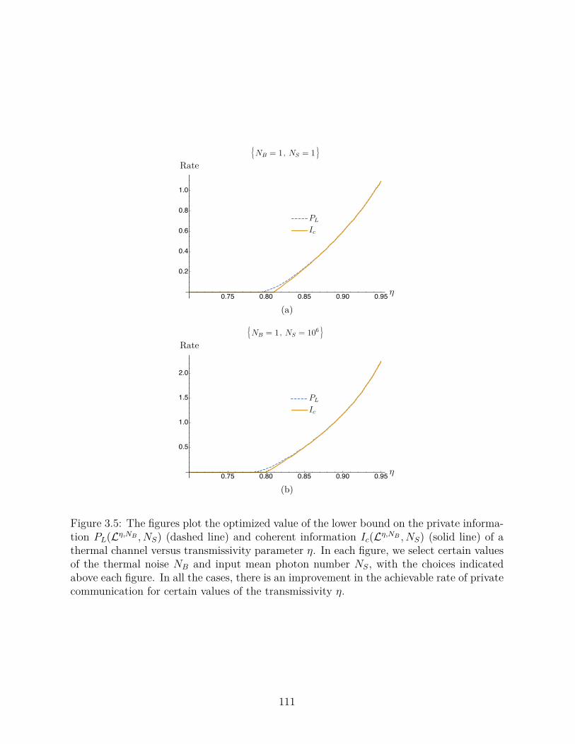
(a)

(b)

Figure 3.5: The figures plot the optimized value of the lower bound on the private informa-

tion PL( Lη ,NB , NS) (dashed line) and coherent information Ic( Lη ,NB , NS) (solid line) of a

thermal channel versus transmissivity parameter η . In each figure, we select certain values

of the thermal noise NB

and input mean photon number NS, with the choices indicated

above each figure. In all the cases, there is an improvement in the achievable rate of private

communication for certain values of the transmissivity η .

111

same form as (3.3.1), i.e.,

Ic( Lη ,NB , NS) = g ( η NS

+ (1 − η ) NB) − g ([ D + (1 − η ) NS

− (1 − η ) NB

− 1] / 2)

− g ([ D − (1 − η ) NS

+ (1 − η ) NB

− 1] / 2) , (3.5.10)

where D2 ≡ [(1+ η ) NS+(1 − η ) NB+1]2 − 4 η NS( NS+1) . Similarly, Ic( Lη ,NB , N2

S) is defined

by replacing NS

in (3.5.10) with N2

S.

We optimize the lower bound in (3.5.9) on the private information PL( Lη ,NB , NS) with

respect to N2

S

for a fixed value of NS

[163]. In Figure 3.5, we plot the optimized value of

the lower bound in (3.5.9) on the private information PL( Lη ,NB , NS) (dashed line) and the

coherent information in (3.5.10) Ic( Lη ,NB , NS) (solid line) of the thermal channel versus

the transmissivity parameter η , for low thermal noise NB

and for both low and high input

mean number of photons NS. We find that a larger rate for private communication can

be achieved by using displaced thermal states as input to the channel instead of coherent

states, for certain values of the transmissivity η .

3.6 Upper Bounds on Energy-Constrained Quantum and Private Capacities

of Quantum Amplifier Channels

Using methods similar to those from Sections 3.2 and 3.4, we now establish three

different upper bounds on the energy-constrained quantum and private capacities of a

noisy amplifier channel.

3.6.1 Data-Processing Bound on Energy-Constrained Quantum and Private

Capacities of Quantum Amplifier Channels

In this section, we establish an upper bound on the energy-constrained quantum and

private capacities by invoking Theorem 83 and a data-processing argument to a noisy

amplifier channel AG,NB with gain G > 1 , environment photon number NB

≥ 0 , for which

τ = G and ν = ( G − 1)(2 NB+1) . This channel is entanglement-breaking when ( G − 1) NB

≥

1 [126].

112

Theorem 93 An upper bound on the energy-constrained quantum and private capacities of

a noisy amplifier channel AG,NB with gain G > 1 and environment photon number NB

≥ 0 ,

such that ( G − 1) NB

< 1 , and input photon number constraint NS

≥ 0 , is given by

Q ( AG,NB , NS) , P ( AG,NB , NS) ≤ max 0 , QU1( AG,NB , NS) ,

(3.6.1)

where

QU1( AG,NB , NS) ≡ g ( G′ NS

+ G′ − 1) − g [( G′ − 1)( NS

+ 1)] , (3.6.2)

G′ = G/ (1 + NB(1 − G )) . (3.6.3)

Proof. An upper bound on the energy-constrained quantum and private capacities can be

established by using (3.2.70) and a data-processing argument. We find that

Q ( AG,NB , NS) = Q ( Lη , 0 AG′ , 0 , NS) (3.6.4)

≤ Q ( AG′ , 0 , NS) (3.6.5)

= max 0 , g ( G′ NS

+ G′ − 1) − g [( G′ − 1)( NS

+ 1)] . (3.6.6)

The first inequality follows from the definition and data processing—the energy-constrained

capacity of Lη , 0 AG′ , 0 cannot exceed that of AG′ , 0. The second equality follows from

the formula for the energy-constrained quantum capacity of a quantum-limited amplifier

channel with gain G′ and input mean photon number NS

[65]. Since a quantum-limited

amplifier channel is a degradable channel [160,171], its energy-constrained private capacity

is the same as its energy-constrained quantum capacity.

Remark 94 Applying Remark 65, we find the following data-processing bound QU1( AG,NB )

on the unconstrained quantum and private capacities of amplifier channels for which ( G −

113

1) NB

< 1 :

Q ( AG,NB ) , P ( AG,NB ) ≤ QU1( AG,NB ) = sup

NS : NS

∈ [0 , ∞ ]

QU1( AG,NB , NS) (3.6.7)

= lim

NS

→∞

QU1( AG,NB , NS) (3.6.8)

= log2( G/ ( G − 1)) − log2( NB

+ 1) . (3.6.9)

The second equality follows from the monotonicity of QU1( AG,NB , NS) with respect to NS,

which in turn follows from the fact that the first derivative of QU1( AG,NB , NS) with respect

to NS

goes to zero as NS

→ ∞ , and the second derivative is always negative.

The bound

Q ( AG,NB ) , P ( AG,NB ) ≤ log2

(

GNB+1

G − 1

)

− g ( NB)

(3.6.10)

was given in [161,162]. From a comparison of (3.6.9) with (3.6.10) , we find that the bound

given in (3.6.10) is always tighter than (3.6.9) . Both the bounds in (3.6.9) and (3.6.10)

converge to the true unconstrained quantum and private capacity in the limit as NB

→ 0 ,

but (3.6.10) is tighter for NB

> 0 .

Remark 95 The data-processing bound QU1( AG,NB , NS) on the energy-constrained quan-

tum capacity of amplifier channels places a strong restriction on the channel parameters

G and NB. Since the quantum capacity of a quantum-limited amplifier channel with gain

G′ is non-zero only for G′ = ∞ , the energy-constrained quantum capacity of an amplifier

channel will be non-zero only for

1 ≤ G < (1 + NB) /NB

, (3.6.11)

which is same as the condition given in [127] and is equivalent to the condition ( G − 1) NB

<

1 , that the channel is not entanglement breaking.

We now study the closeness of the data-proccessing bound QU1( AG,NB , NS) when compared

114

to a known lower bound. In particular, we use the following lower bound on the energy-

constrained quantum and private capacities of an amplifier channel [62,147] and denote it

by QL( AG,NB , NS) :

Q ( AG,NB , NS) ≥ QL( AG,NB , NS) ≡ g ( GNS

+ ( G − 1)( NB

+ 1))

− g ([ D + ( G − 1)( NS

+ NB

+ 1) − 1] / 2) − g ([ D − ( G − 1)( NS

+ NB

+ 1) − 1] / 2) ,

(3.6.12)

where

D2 ≡ [(1 + G ) NS

+ ( G − 1)( NB

+ 1) + 1]2 − 4 GNS( NS

+ 1) .

(3.6.13)

Theorem 96 Let AG,NB be an amplifier channel with gain G > 1 and environment photon

number NB

≥ 0 , such that ( G − 1) NB

< 1 , and input photon number constraint NS

≥ 0 .

Then the following relation holds between the data-processing bound QU1( AG,NB , NS) in

(3.6.1) and the lower bound QL( AG,NB , NS) in (3.6.12) on the energy-constrained quantum

and private capacities of an amplifier channel:

QL( AG,NB , NS) ≤ QU1( AG,NB , NS) ≤ QL( AG,NB , NS) + 1 / ln 2 . (3.6.14)

Proof. A proof follows from arguments similar to those in the proof of Theorem 87.

3.6.2 ε -Degradable Bound on Energy-Constrained Quantum and Private Ca-

pacities of Amplifier Channels

In this section, we provide an upper bound on the energy-constrained quantum and

private capacities of a quantum amplifier channel AG,NB using the idea of ε -degradability.

We first construct an approximate degrading channel D by following arguments similar

115

to those in Section 3.2.2. Furthermore, we introduce a particular channel that simulates

the serial concatenation of the amplifier channel AG,NB and the approximate degrading

channel D . We finally provide an upper bound on the energy-constrained quantum and

private capacities of an amplifier channel by using all these tools and invoking Theorem 68.

Similar to Section 3.2.2, we first establish an upper bound on the diamond distance

between the complementary channel of the amplifier channel and the concatenation of the

amplifier channel followed by a particular approximate degrading channel. Let T and

T

′ represent transformations of two-mode squeezers with parameter G and (2 G − 1) /G ,

respectively. In the Heisenberg picture, the unitary transformation corresponding to T and

T

′ follow from (2.3.82).

Consider the following action of the noisy amplifier channel AG,NB on an input state

ϕR A:

(idR

⊗AG,NB )( ϕR A) = TrE1

E2

TAE

′ → B E2( ϕR A

⊗ ψTMS( NB)E

′ E1) ,

(3.6.15)

where R is a reference system and ψTMS( NB)E

′ E1

is a two-mode squeezed vacuum state

with parameter NB, as defined in (2.3.34). It is evident from (3.6.15) that the output

of the noisy amplifier channel AG,NB is system B , and the outputs of the complementary

channel AG,NB

are systems E1

and E2.

Consider a two-mode squeezer T

′ with parameter (2 G − 1) /G , such that the output

of the amplifier channel AG,NB becomes an environmental input for T

′. We consider one

mode of the two-mode squeezed vacuum state ψTMS( NB)F E

′

1

as an input for T

′, so that

the subsystem E

′

1

mimics E1. We denote our choice of degrading channel by D(2 G − 1) /G,NB

:

T ( B ) → T ( E

′

1

E

′

2) . More formally, D(2 G − 1) /G,NB

has the following action on the output

state AG,NB ( ϕR A) :

(idR

⊗ [ D(2 G − 1) /G,NB

AG,NB ])( ϕR A) = Tr G

T

′

B F → E

′

2

G( AG,NB ( ϕR A) ⊗ ψTMS( NB)F E

′

1)) .

(3.6.16)

116

Now, similar to Section 3.2.2, we introduce a particular channel that simulates the

action of D(2 G − 1) /G

AG,NB on an input state ϕR A. We denote this channel by Λ , and it

has the following action on an input state ϕR A:

(idR

⊗ Λ)( ϕR A) = Tr B

TAE

′ → B E2( ϕR A

⊗ ω ( NB)E

′ E1) ,

(3.6.17)

where ω ( NB)E

′ E1

represents a noisy version of a two-mode squeezed vacuum state with

parameter NB, and is the same as (3.2.25), except η is replaced by G . Similar to (3.2.26),

the following equivalence holds for any quantum input state ϕR A:

(idR

⊗ [ D(2 G − 1) /G,NB

AG,NB ])( ϕR A) = (idR

⊗ Λ)( ϕR A) .

(3.6.18)

Thus, the channels D(2 G − 1) /G,NB

AG,NB and Λ are indeed the same.

Similar to Theorem 76, we now establish an upper bound on the diamond distance

between the complementary channel of a noisy amplifier channel and the concatenation of

the amplifier channel followed by the degrading channel in (3.6.16).

Theorem 97 Fix G > 1 . Let AG,NB be an amplifier channel with gain G , and let D(2 G − 1) /G,NB

be a degrading channel as defined in (3.6.16) . Then

1

2

∥ AG,NB

− D(2 G − 1) /G,NB

AG,NB ∥⋄

≤

√

1 − G2 /κ ( G, NB) ,

(3.6.19)

with

κ ( G, NB) = G2 + NB( NB

+ 1)[1 + 3 G2 − 2 G (1 +

√

2 G − 1)] .

(3.6.20)


Theorem 98 An upper bound on the energy-constrained quantum capacity of a noisy

amplifier channel AG,NB with gain G > 1 , environment photon number NB, such that

117

( G − 1) NB

< 1 , and input mean photon-number constraint NS

≥ 0 is given by

Q ( AG,NB , NS) ≤ QU2( AG,NB , NS) ≡ g ( GNS

+ ( G − 1) NB) − g ( ζ+) − g ( ζ−)

+ (2 ε′ + 4 δ ) g ([( G − 1) NS

+ (1 + G ) NB] /δ ) + g ( ε′) + 2 h2( δ ) , (3.6.21)

with

ε =

√

1 − G2 /

(

G2 + NB( NB

+ 1)[1 + 3 G2 − 2 G (1 +

√

2 G − 1)]

)

, (3.6.22)

ζ±

=

1

2

(

− 1 +

√

[(1 + 2 NB)2 − 2 ϱ + (2 ϑ − 1)2 ± 4( ϑ − NB

− 1)

√

[ NB

+ ϑ ]2 − ϱ ] / 2

)

,

(3.6.23)

ϱ = 4 NB( NB

+ 1)(2 G − 1) /G , (3.6.24)

ϑ = G (1 + NB) + ( G − 1) NS

, (3.6.25)

ε′ ∈ ( ε, 1] , and δ = ( ε′ − ε ) / (1 + ε′) .


Theorem 99 An upper bound on the energy-constrained private capacity of a noisy am-

plifier channel AG,NB with gain G > 1 , environment photon number NB, such that ( G −

1) NB


≥ 0 is given by

P ( AG,NB , NS) ≤ PU2( AG,NB , NS) ≡ g ( GNS

+ ( G − 1) NB) − g ( ζ+) − g ( ζ−)

+ (6 ε′ + 12 δ ) g ([( G − 1) NS

+ (1 + G ) NB] /δ ) + 3 g ( ε′) + 6 h2( δ ) , (3.6.26)

118

with

ε =

√

1 − G2 /

(

G2 + NB( NB

+ 1)[1 + 3 G2 − 2 G (1 +

√

2 G − 1)]

)

, (3.6.27)

ζ±

=

1

2

(

− 1 +

√

[(1 + 2 NB)2 − 2 ϱ + (2 ϑ − 1)2 ± 4( ϑ − NB

− 1)

√

[ NB

+ ϑ ]2 − ϱ ] / 2

)

,

(3.6.28)

ϱ = 4 NB( NB

+ 1)(2 G − 1) /G , (3.6.29)

ϑ = G (1 + NB) + ( G − 1) NS

, (3.6.30)

ε′ ∈ ( ε, 1] , and δ = ( ε′ − ε ) / (1 + ε′) .



3.6.3 ε -Close-Degradable Bound on Energy-Constrained Quantum and Pri-

vate Capacities of Amplifier Channels

In this section, we first establish an upper bound on the diamond distance between

a noisy amplifier channel and a quantum-limited amplifier channel. Since a quantum-

limited amplifier channel is a degradable channel, an upper bound on the energy-constrained

quantum capacity of a noisy amplifier channel directly follows from Theorem 69.

Theorem 100 If a noisy amplifier channel AG,NB and a quantum-limited amplifier channel

AG, 0 have the same gain G > 1 , then

1

2

∥∥∥ AG,NB − AG, 0

∥∥∥⋄

≤

NB

NB

+ 1

.

(3.6.31)


Theorem 101 An upper bound on the energy-constrained quantum capacity of a noisy

amplifier channel AG,NB with gain G > 1 , environment photon number NB, such that

119

( G − 1) NB


≥ 0 is given by

Q ( AG,NB , NS) ≤ QU3( AG,NB , NS) ≡ g ( GNS

+ G − 1) − g [( G − 1)( NS

+ 1)]

+ (4 ε′ + 8 δ ) g [( GNS

+ ( G − 1) NB) /δ ] + 2 g ( ε′) + 4 h2( δ ) , (3.6.32)

with ε = NB

/ ( NB

+ 1) , ε′ ∈ ( ε, 1] and δ = ( ε′ − ε ) / (1 + ε′) .


Theorem 102 An upper bound on the energy-constrained private capacity of a noisy am-

plifier channel AG,NB with gain G > 1 , environment photon number NB, such that ( G −

1) NB


≥ 0 is given by

P ( AG,NB , NS) ≤ PU3( AG,NB , NS) ≡ g ( GNS

+ G − 1) − g [( G − 1)( NS

+ 1)]

+ (8 ε′ + 16 δ ) g [( GNS

+ ( G − 1) NB) /δ ] + 4 g ( ε′) + 8 h2( δ ) , (3.6.33)

with ε = NB

/ ( NB

+ 1) , ε′ ∈ ( ε, 1] and δ = ( ε′ − ε ) / (1 + ε′) .



3.7 Upper Bounds on Energy-Constrained Quantum and Private Capacities

of Additive-Noise Channels

In this section, we provide upper bounds on the energy-constrained quantum and pri-

vate capacities of an additive-noise channel using Theorems 73 and 84. Note that we only

consider ξ ∈ (0 , 1) because the additive-noise channel is not entanglement breaking in this

interval [126]. The additive-noise channel with noise paramter ξ was defined in (2.3.85).

Theorem 103 An upper bound on the energy-constrained quantum and private capacities

of an additive-noise channel T

ξ with noise parameter ξ ∈ (0 , 1) , and input mean photon

120


is given by

Q ( T

ξ , NS) , P ( T

ξ , NS) ≤ max 0 , QU1( T

ξ , NS) ,

(3.7.1)

where

QU1( T

ξ , NS) ≡ g ( NS

/ ( ξ + 1)) − g ( ξ NS

/ ( ξ + 1)) .

(3.7.2)

Proof. A proof follows from the fact that an additive noise channel can be obtained from

a thermal noise channel in the limit η → 1 and NB

→ ∞ , with (1 − η ) NB

→ ξ [172],

as well by applying the continuity results for these capacities from [173, Theorem 3] (see

also [138]). By taking these limits in (3.2.3), we obtain the desired result.

Remark 104 Applying Remarks 65 and 74, and Theorem 103, we find the following data-

processing bound QU1( T

ξ) on the unconstrained quantum and private capacities of additive-

noise channels for ξ ∈ (0 , 1) :

QU1( T

ξ) = log2(1 /ξ ) .

(3.7.3)

Remark 105 From Theorem 87, it follows that the data-processing upper bound Q ( T

ξ , NS)

can be at most 1.45 bits larger than a known lower bound on the energy-constrained quantum

and private capacities of an additive-noise channel.

Remark 106 The following bound was given in [161,162] for ξ ∈ (0 , 1) :

Q ( T

ξ) , P ( T

ξ) ≤

ξ − 1

ln 2

+ log2(1 /ξ ) .

(3.7.4)

From a comparison of (3.7.3) with the bound in (3.7.4) , we find that the bound in (3.7.4)

is always tighter than (3.7.3) .

We now establish another upper bound on the energy-constrained quantum and private

capacities of an additive-noise channel, by using Theorem 84.

121

Theorem 107 An upper bound on the energy-constrained quantum and private capacities

of an additive-noise channel T

ξ with noise parameter ξ ∈ (0 , 1) , and input photon number

constraint NS

≥ 0 is given by

Q ( T

ξ , NS) , P ( T

ξ , NS) ≤ max 0 , QU4( T

ξ , NS) ,

(3.7.5)

where

QU4( T

ξ , NS) ≡ g ( NS

+ ξ ) − g [ ξ ( NS

+ ξ ) / (1 − ξ )] .

(3.7.6)



Remark 108 From a comparision of (3.7.6) and (3.7.2) , we find that QU1( T

ξ , NS) is

tighter than QU4( T

ξ , NS) only for low noise and low input mean photon number. The

bound QU4( T

ξ , NS) is tighter than QU1( T

ξ , NS) for all other parameter regimes.

Remark 109 Applying Remarks 65 and 74, and Theorem 107, we find the following data-

processing bound QU4( T

ξ) on the unconstrained quantum and private capacities of additive-

noise channels:

QU4( T

ξ) = log2[(1 − ξ ) /ξ ] .

(3.7.7)

Remark 110 From a comparison of (3.7.7) with the bound in (3.7.4) , we find that (3.7.7)

is tighter than (3.7.4) for high noise.

3.8 On the Optimization of Generalized Channel Divergences of Quantum

Gaussian Channels

In this section, we address the question of computing the energy-constrained diamond

norm of several channels of interest that have appeared in this dissertation. We provide a

very general argument, based on some definitions and results in [153] and phrased in terms

of the “generalized channel divergence” as a measure of the distinguishability of quantum

122

channels. We find that, among all Gaussian input states with a fixed energy constraint, the

two-mode squeezed vacuum state saturating the energy constraint is an optimal state for

the energy-constrained generalized channel divergence of two particular Gaussian channels.

We describe these results in more detail in what follows.

We begin by recalling some developments from [153]:

Definition 111 (Generalized divergence [174, 175]) A functional D : D ( H ) ×D ( H ) →

R is a generalized divergence if it satisfies the monotonicity (data processing) inequality

D ( ρ ∥ σ ) ≥ D ( N ( ρ ) ∥N ( σ )) ,

(3.8.1)

where N is a quantum channel.

Particular examples of a generalized divergence are the trace distance, quantum relative

entropy, and the negative root fidelity.

We say that a generalized channel divergence possesses the direct-sum property on

classical–quantum states if the following equality holds:

D

(∑

x

pX( x ) | x ⟩⟨ x |X

⊗ ρx

∥∥∥∥∥

∑

x

pX( x ) | x ⟩⟨ x |X

⊗ σ

x

)

=

∑

x

pX( x ) D ( ρx ∥ σ

x) ,

(3.8.2)

where pX

is a probability distribution, | x ⟩x

is an orthonormal basis, and ρx x

and σ

x x

are sets of states. We note that this property holds for trace distance, quantum relative

entropy, and the negative root fidelity.

Definition 112 (Generalized channel divergence [153]) Given quantum channels NA → B

and MA → B, we define the generalized channel divergence as

D ( N ∥M ) ≡ sup

ρR A

D ((idR

⊗NA → B)( ρR A) ∥ (idR

⊗MA → B)( ρR A)) .

(3.8.3)

In the above definition, the supremum is with respect to all mixed states and the reference

system R is allowed to be arbitrarily large. However, as a consequence of purification, data

123

processing, and the Schmidt decomposition, it follows that

D ( N ∥M ) = sup

ψR A

D ((idR

⊗NA → B)( ψR A) ∥ (idR

⊗MA → B)( ψR A)) ,

(3.8.4)

such that the supremum can be restricted to be with respect to pure states and the reference

system R isomorphic to the channel input system A .

Particular cases of the generalized channel divergence are the diamond norm of the

difference of NA → B

and MA → B

as well as the Rényi channel divergence from [176].

Covariant quantum channels have symmetries that allow us to simplify the set of states

over which we need to optimize their generalized channel divergence [177]. Let G be a finite

group, and for every g ∈ G , let g → UA( g ) and g → VB( g ) be unitary representations acting

on the input and output spaces of the channel, respectively. Then a quantum channel NA → B

is covariant with respect to ( UA( g ) , VB( g )) g

if the following relation holds for all input

density operators ρA

and group elements g ∈ G :

( NA → B

U

g

A) ( ρA) = ( V

g

B

NA → B) ( ρA) ,

(3.8.5)

where

U

g

A( ρA) = UA( g ) ρA

U

†

A( g ) , (3.8.6)

V

g

B( σB) = VB( g ) σB

V

†

B( g ) . (3.8.7)

We say that channels NA → B

and MA → B

are jointly covariant with respect to ( UA( g ) , VB( g )) g ∈ G

if each of them is covariant with respect to ( UA( g ) , VB( g )) g

[168,178].

The following lemma was established in [153]:

Lemma 4 (Lemma II.3, [153]) Let NA → B

and MA → B

be quantum channels, and let

( UA( g ) , VB( g )) g ∈ G

denote unitary representations of a group G . Let ρA

be a density

124

operator, and let ϕρ

R A

be a purification of ρA. Let ¯ ρA

denote the group average of ρA

according to a distribution pG, i.e.,

¯ ρA

=

∑

g

pG( g ) U

g

A( ρA) ,

(3.8.8)

and let ϕ¯ ρ

R A

be a purification of ¯ ρA. If the generalized divergence possesses the direct-sum

property on classical–quantum states, then the following inequality holds

D ( NA → B( ϕ¯ ρ

R A) ∥MA → B( ϕ¯ ρ

R A))

≥

∑

g

pG( g ) D

((

V

g †

B

NA → B

U

g

A

)

( ϕρ

R A)

∥∥∥

(

V

g †

B

MA → B

U

g

A

)

( ϕρ

R A)

)

. (3.8.9)

By approximation, the above lemma can be extended to continuous groups for several

generalized channel divergences of interest:

Lemma 5 Let NA → B

and MA → B

be quantum channels, and let ( UA( g ) , VB( g )) g ∈ G

de-

note unitary representations of a continuous group G . Let ρA

be a density operator, and let

ϕρ

R A

be a purification of ρA. Let ¯ ρA

denote the group average of ρA

according to a measure

µ ( g ) , i.e.,

¯ ρA

=

∫

dµ ( g ) U

g

A( ρA) ,

(3.8.10)

and let ϕ¯ ρ

R A

be a purification of ¯ ρA. If the generalized divergence possesses the direct-sum

property on classical–quantum states and is a Borel function, then the following inequality

holds

D ( NA → B( ϕ¯ ρ

R A) ∥MA → B( ϕ¯ ρ

R A))

≥

∫

dµ ( g ) D

((

V

g †

B

NA → B

U

g

A

)

( ϕρ

R A)

∥∥∥

(

V

g †

B

MA → B

U

g

A

)

( ϕρ

R A)

)

. (3.8.11)

125

We can apply this lemma effectively in the context of quantum Gaussian channels. To

this end, we consider an energy-constrained generalized channel divergence for W ∈ [0 , ∞ )

and an energy observable G as follows:

DG,W ( N ∥M ) = sup

ψR A

: Tr GψA

≤ W

D ((idR


⊗MA → B)( ψR A)) .

(3.8.12)

In what follows, we specialize this measure even further to the Gaussian energy-constrained

generalized channel divergence, meaning that the optimization is constrained to be with

respect to Gaussian input states:

DG

G,W ( N ∥M ) = sup

ψR A

: Tr GψA

≤ W, ψR A

∈GD ((idR


⊗MA → B)( ψR A)) ,

(3.8.13)

where G denotes the set of Gaussian states. We then establish the following proposition:

Proposition 113 Suppose that channels NA → B

and MA → B

are Gaussian, they each take

one input mode to m output modes, and they have the following action on a single-mode,

input covariance matrix V :

V → X V X

T + YN

, (3.8.14)

V → X V X

T + YM

, (3.8.15)

where X is an m × 1 matrix, YN

and YM

are m × m matrices such that NA → B

and MA → B

are legitimate Gaussian channels. Suppose furthermore they these channels are jointly

phase covariant (phase-insensitive), in the sense that for all ϕ ∈ [0 , 2 π ) and input density

operators ρ , the following equality holds

NA → B( ei ˆ nϕ ρe− i ˆ nϕ) =

(

m⊗

i =1


)

NA → B( ρ )

(

m⊗

i =1


)

, (3.8.16)

MA → B( ei ˆ nϕ ρe− i ˆ nϕ) =

(

m⊗

i =1


)

MA → B( ρ )

(

m⊗

i =1


)

, (3.8.17)

126

where ai

∈ 0 , 1 for i ∈ 1 , . . . , m and ˆ ni

is the photon number operator for the i th mode.

Then it suffices to restrict the optimization in the energy-constrained generalized channel

divergence as follows:

Dˆ n,NS( N ∥M ) = sup

ψR A:Tr ˆ nψA

= NS

D ((idR

⊗NA → B) ( ψR A) ∥ (idR

⊗MA → B) ( ψR A)) ,

(3.8.18)

where ψR A

= | ψ ⟩⟨ ψ |R A

and

| ψ ⟩R A

=

∞∑

n =0

λn

| n ⟩R

| n ⟩A

,

(3.8.19)

for some λn

∈ R+ such that

∑∞

n =0

λ2

n

= 1 and

∑∞

n =0

nλ2

n

= NS. Furthermore, the Gaussian

energy-constrained generalized channel divergence is achieved by the two-mode squeezed

vacuum state with parameter NS, i.e.,

DG

ˆ n,NS( N ∥M ) = D ((idR

⊗NA → B) ( ψTMS( NS)) ∥ (idR

⊗MA → B) ( ψTMS( NS))) .

(3.8.20)

Proof. This result is an application of Lemma 5 and previous developments in this

dissertation. We first exploit the joint displacement covariance of the channels NA → B

and MA → B. That is, the fact that channels NA → B

and MA → B

have the same X ma-

trix as given in (3.8.14)–(3.8.15) implies that they are jointly covariant with respect to

displacements; i.e., for all input density operators ρ and unitary displacement operators

D ( α ) ≡ exp

(

α ˆ a† − α

∗ˆ a

)

, the following equalities hold

NA → B( D ( α ) ρD ( − α )) =

(

m⊗

i =1

D ( fi( X , α ))

)

NA → B( ρ )

(

m⊗

i =1

D ( − fi( X , α ))

)

, (3.8.21)

MA → B( D ( α ) ρD ( − α )) =

(

m⊗

i =1

D ( fi( X , α ))

)

MA → B( ρ )

(

m⊗

i =1

D ( − fi( X , α ))

)

, (3.8.22)

where fi

for i ∈ 1 , . . . , m are functions depending on the entries of the matrix X and α .

Let ϕR A

be an arbitrary pure state such that Tr ˆ nϕA

= N1

≤ NS. Consider the following

127

additive-noise Gaussian channel acting on an input state ρA:

A ( ρA) =

∫

d2 α pN2( α ) D ( α ) ρA

D ( − α ) ,

(3.8.23)

where pN2( α ) = exp − | α |2 /N2

/π N2

is a complex, centered Gaussian probability density

function with variance N2

≡ NS

− N1

≥ 0 . Applying this channel to ϕA

increases its photon

number from N1

to NS:

Tr ˆ n A ( ϕA) = NS

,

(3.8.24)

which follows because

Tr ˆ n A ( ϕA) = Tr ˆ a†ˆ a

∫

d2 α pN2( α ) D ( α ) ϕA

D ( − α ) (3.8.25)

=

∫

d2 α pN2( α ) Tr D ( − α )ˆ a†ˆ aD ( α ) ϕA

(3.8.26)

=

∫

d2 α pN2( α ) Tr D ( − α )ˆ a† D ( α ) D ( − α )ˆ aD ( α ) ϕA

(3.8.27)

=

∫

d2 α pN2( α ) Tr [ˆ a† + α

∗][ˆ a + α ] ϕA

(3.8.28)

=

∫

d2 α pN2( α )

[

Tr ˆ a†ˆ aϕA

+ α Tr ˆ a† ϕA

+ α

∗ Tr ˆ aϕA

+ | α |2 Tr ϕA

]

(3.8.29)

= N1

+ 0 + 0 + N2

= NS

. (3.8.30)

The first three equalities use definitions, cyclicity of trace, and the fact that D ( α ) D ( − α ) =

I . The fourth equality uses the well known identities (see, e.g., [68])

D ( − α )ˆ aD ( α ) = ˆ a + α , D ( − α )ˆ a† D ( α ) = ˆ a† + α

∗ .

(3.8.31)

The second-to-last equality follows because pN2( α ) is a probability density function with

mean zero and variance N2

(we have explicitly indicated what each of the four terms

evaluate to in the following line). Let φR A

denote a purification of the state A ( ϕA) . We

can then exploit the joint covariance of the channels with respect to displacements, the

128

relation in (3.8.23), and Lemma 5 to conclude that

D ( NA → B( φR A) ∥MA → B( φR A)) ≥ D ( NA → B( ϕR A) ∥MA → B( ϕR A)) ,

(3.8.32)

for all N1

≤ NS. As a consequence of this development, we find that it suffices to restrict

the optimization of the energy-constrained, generalized channel divergence to pure bipartite

states φR A

that meet the energy constraint with equality (i.e., Tr ˆ nφA

= NS).

Now we exploit the joint phase covariance of the channels. Let φR A

be a pure bipartite

state that meets the energy constraint with equality. Consider that

φA

≡

1

2 π

∫ 2 π

0

dϕ ei ˆ nϕ φA

e− i ˆ nϕ =

∞∑

n =0

| n ⟩⟨ n | φA

| n ⟩⟨ n | .

(3.8.33)

That is, the state after phase averaging is diagonal in the number basis, and furthermore,

the resulting state

φA

has the same photon number NS

as φA

because

Tr ˆ n

φA

=

1

2 π

∫ 2 π

0

dϕ Tr ˆ nei ˆ nϕ φA

e− i ˆ nϕ (3.8.34)

=

1

2 π

∫ 2 π

0

dϕ Tr e− i ˆ nϕˆ nei ˆ nϕ φA

(3.8.35)

=

1

2 π

∫ 2 π

0

dϕ Tr ˆ nφA

= Tr ˆ nφA

. (3.8.36)

Thus,

φA

=

∑∞

n =0

λ2

n

| n ⟩⟨ n |A, for some λn

∈ R+ such that

∑∞

n =0

λ2

n

= 1 and

∑∞

n =0

nλ2

n

= NS.

Let ξR A

denote a pure bipartite state that purifies

φA. By applying Lemma 5 and the joint

phase covariance relations in (3.8.16)–(3.8.17), we find that the following inequality holds

D ( NA → B( ξR A) ∥MA → B( ξR A)) ≥ D ( NA → B( φR A) ∥MA → B( φR A)) .

(3.8.37)

Since all purifications are related by isometries acting on the purifying system R , and since

129

a generalized divergence is invariant under such an isometry [179], we find that

D ( NA → B( ξR A) ∥MA → B( ξR A)) = D ( NA → B( ψR A) ∥MA → B( ψR A)) ,

(3.8.38)

where ψR A

is a state of the form in (3.8.19). This concludes the proof of (3.8.18).

To conclude (3.8.20), consider that the thermal state θ ( NS) is the only Gaussian state

of a single mode that is diagonal in the number basis with photon number equal to NS. A

purification of the thermal state θ ( NS) is the two-mode squeezed vacuum ψTMS( NS) with

parameter NS. So this means that, for a fixed photon number NS, the two-mode squeezed

vacuum with parameter NS

is optimal among all Gaussian states with reduced state on the

channel input having the same photon number.

We note here that joint phase covariance of two otherwise arbitrary channels implies

that states of the form in (3.8.19) with mean photon number of their reduced states ≤

NS

are optimal, while joint displacement covariance of two otherwise arbitrary channels

implies that states with mean photon number of their reduced states = NS

are optimal.

In Proposition 113, we chose to present the interesting case of Gaussian channels in which

both kinds of joint covariance hold simultaneously. The aforementioned result regarding

jointly phase-covariant channels was concluded in [180] for a special case by employing a

different argument and considering the special case of fidelity and Chernoff-information

divergences, as well as the discrimination of pure-loss channels. It is worthwhile to note

that our argument is different, relying mainly on channel symmetries and data processing,

and thus applies in far more general situations than those considered in [180].

Proposition 113 applies to the various settings and channels that we have considered in

this dissertation for ε -degradable and ε -close degradable bosonic thermal channels. Thus,

we can conclude in these situations that the Gaussian energy-constrained generalized chan-

nel divergence is achieved by the two-mode squeezed vacuum state.

Particular generalized channel divergences of interest are the energy-constrained di-

130

amond norm [137, 138] and the energy-constrained, channel version of the C -distance

[130,132,133,181], respectively defined as

∥N − M∥ ,G,W

≡ sup

ψR A

: Tr GψA

≤ W

∥ (idR

⊗NA → B)( ψR A) − (idR

⊗MA → B)( ψR A) ∥1

,

(3.8.39)

CG,W ( N , M ) ≡ sup

ψR A

: Tr GψA

≤ W

√

1 − F ((idR

⊗NA → B)( ψR A) , (idR

⊗MA → B)( ψR A)) ,

(3.8.40)

where F denotes the quantum fidelity. Proposition 113 implies that the Gaussian-constrained

versions of these quantities reduce to the following for channels satisfying the assumptions

stated there:

∥N − M∥G

, ˆ n,NS

= ∥ (idR

⊗NA → B)( ψTMS( NS)) − (idR

⊗MA → B)( ψTMS( NS)) ∥1

, (3.8.41)

C

G

ˆ n,NS( N , M ) =

√

1 − F ((idR

⊗NA → B)( ψTMS( NS)) , (idR

⊗MA → B)( ψTMS( NS))) .

(3.8.42)

We note that the latter quantity is readily expressed as a closed formula in terms of the

Gaussian specification of the channels NA → B

and MA → B

in (3.8.14)–(3.8.15) and the pa-

rameter NS

by employing the general formula for the fidelity of zero-mean Gaussian states

from [182]. One could also employ the formulas from [183] or [184, 185] to compute Gaus-

sian, energy-constrained channel divergences based on Rényi relative entropy or quantum

relative entropy, respectively.

The result in (3.8.18) already significantly reduces the set of states that we need to

consider in computing a given energy-constrained, generalized channel divergence for chan-

nels satisfying the conditions of Proposition 113. However, it is a very interesting open

question to determine whether, under the conditions given in Proposition 113, the energy-

constrained generalized channel divergence is always achieved by the two-mode squeezed

vacuum state (if the restriction to Gaussian input states is lifted). Divergences of interest

131

in applications are the trace distance, fidelity, quantum relative entropy, and Rényi rela-

tive entropies. All of these measures lead to a very interesting suite of Gaussian optimizer

questions, which we leave for future work. If there is a positive answer to this question,

then we would expect to see, in the low-photon-number regime, significant improvements

of the ε -degradable and ε -close degradable upper bounds on the capacities of the thermal

channel.

In the following remark we provide an example where the two-mode squeezed vac-

uum state is not optimal to distinguish two particular Gaussian channels satisfying condi-

tions of Proposition 113 with respect to the energy-constrained channel fidelity. Thus the

aforementioned suggestion does not hold for all the energy-constrained generalized channel

divergences to distinguish two Gaussian channels satisfying Proposition 113.

Remark 114 In Chapter 5 we prove that the optimal state to distinguish an identity chan-

nel I from an additive-noise channel T

ξ with respect the energy-constrained channel fidelity

is an entangled superposition of twin-Fock states. In general, these states are non-Gaussian

quantum states. Note that both I and T

ξ are Gaussian channels with the same X matri-

ces and are jointly phase covariant. Thus, in general, two-mode squeezed vacuum states

saturating the energy constraints are not optimal to distinguish two Gaussian channels sat-

isfying Proposition 113. An interesting question is to determine whether a similar result

holds for the energy-constrained diamond distance between two Gaussian channels in the

context of the approximate degradability bounds introduced in this chapter.

3.9 Conclusion

In this chapter, we established several bounds on the energy-constrained quantum and

private capacities of single-mode, phase-insensitive bosonic Gaussian channels. The energy-

constrained bounds imply bounds for the corresponding unconstrained capacities.

In particular, we began by proving several different upper bounds on the energy-

constrained quantum capacity of thermal channels. We discussed the closeness of these

132

four upper bounds with a known lower bound. In particular, we have shown that the ε -

close degradable bound works well only in the low-noise regime and that the data-processing

and bottleneck upper bounds are close to a lower bound for both low and high thermal

noise. We also discussed an interesting case in which the ε -degradable bound is tighter than

all other upper bounds. We speculate that the ε -degradable bound can be further tightened

by estimating the energy-constrained diamond distance between two particular Gaussian

channels that satisfy the conditions in Proposition 113. In Chapters 4 and 5, we develop

techniques to estimate the energy-constrained diamond distance and the energy-constrained

channel fidelity, which can be further used in bounding the quantum and private capacities

of phase-insensitive Gaussian channels. We leave this for future work.

Similarly, we established several different upper bounds on the energy-constrained pri-

vate capacity of thermal channels. We have also shown an improvement in the achievable

rates of private communication through quantum thermal channels by using displaced ther-

mal states as inputs to the channel.

Additionally, we proved several different upper bounds on the energy-constrained quan-

tum and private capacities of quantum amplifier channels. We also established the data-

processing and the bottleneck upper bounds on the energy-constrained quantum and pri-

vate capacities of additive-noise channels. Moreover, in Chapter 5 (see Remark 117) we

briefly summarize a method for establishing an ε -close-degradable bound on capacities of

additive-noise channels.

We also found that the data-processing bound can be at most 1.45 bits larger than a

known lower bound on the energy-constrained quantum and private capacities of all phase-

insensitive Gaussian channels. Moreover, our results establish strong limitations on any

potential superadditivity of the coherent information of a thermal channel in the low-noise

regime.

Since thermal noise is present in almost all communication and optical systems, our re-

sults have implications for quantum computing and quantum cryptography. The knowledge

133

of bounds on quantum capacity can be useful to quantify the performance of distributed

quantum computation between remote locations, and private communication rates are con-

nected to the ability to generate secret keys.

We finally used the generalized channel divergence from [153] to address the question

of optimal input states for the energy-bounded diamond norm and other related diver-

gences. In particular, we showed that for two Gaussian channels that are jointly phase and

displacement covariant, the Gaussian energy-constrained generalized channel divergence is

achieved by a two-mode squeezed vacuum state that saturates the energy constraint. It is

an interesting open question to determine whether, among all input states, the two-mode

squeezed vacuum is the optimal input state for several energy-constrained, generalized

channel divergences of interest. Here, we have reduced the optimization to be as given

in (3.8.18). As discussed in Remark 114, we provide a partial answer to this question by

showing both numerically and analytically that the suggestion mentioned above does not

hold for the task of distinguishing an additive-noise channel from an identity channel with

respect to the energy-constrained sine distance.

134

CHAPTER 4

CHARACTERIZING THE PERFORMANCE OF

CONTINUOUS-VARIABLE GAUSSIAN QUANTUM GATES

In this chapter, we study three different performance criteria to analyze how well ex-

perimental approximations simulate ideal Gaussian operations. We focus on the following

notions of convergence for quantum channels: uniform and strong convergence, and uni-

form convergence on the set of density operators whose marginals on the channel input have

bounded energy (see Section 2.5 in Chapter 2 for more details). We analyze several exper-

imental approximations of particular Gaussian unitaries, such as displacement operators,

phase rotations, beamsplitters, single-mode squeezing operators, and the SUM operation,

which are sufficient to generate an arbitrary Gaussian unitary operation acting on n modes

of the electromagnetic field [74].

We first prove that none of these experimental approximations converge uniformly to

the ideal Gaussian processes. We then show that these experimental approximations of

an ideal displacement operator, beamsplitter, phase rotation, single-mode squeezer, and

SUM gate converge to the ideal unitaries in the strong sense. Since the strong convergence

of a sequence of infinite-dimensional channels is equivalent to uniform convergence on the

set of energy-bounded density operators [137], our results imply that these experimental

approximations of an ideal displacement operator, single-mode squeezer, and SUM gate

converge uniformly to the ideal unitaries on the set of energy-bounded density operators.

In order to experimentally approximate these different unitary operations, it is im-

portant to study how the uniform convergence over the set of energy-bounded operators

depends on different experimental parameters. In particular, we consider the energy-

constrained sine distance [93, Section 12] as a metric to bound the energy-constrained

diamond distance between an ideal displacement operator and its experimental approxi-

mation. We first show that the fidelity between the ideal displacement and its experimental

135

approximation when acting on a fixed input state is equal to the fidelity between a pure-loss

channel and an ideal channel when acting on the same input state. We then provide an

analytical expression to upper bound the energy-constrained diamond distance between an

ideal displacement and its experimental approximations, by using the recent result of [186].

Furthermore, we study different performance metrics to analyze how well an experimental

approximation simulates a tensor product of different displacement operators.

We also establish two different lower bounds on the energy-constrained diamond dis-

tance [137, 138] between an ideal displacement operator and its experimental approxima-

tion by employing two different techniques. A first technique is based on the trace distance

between the outputs of these two channels for a particular choice of the input state. In

particular, we provide an analytical expression for a lower bound on the energy-constrained

diamond distance for low values of the energy constraint. A second technique is to esti-

mate the energy-constrained diamond distance by using a semidefinite program (SDP) on

a truncated Hilbert space. In particular, we use an SDP from [138], which directly follows

from an SDP from [187,188] defined in the context of finite-dimensional quantum channels.

Moreover, we analytically show that for a fixed value of the energy constraint and for a

sufficiently high value of the truncation parameter, the energy-constrained diamond dis-

tance between two quantum channels can be estimated with an arbitrarily high accuracy

by using an SDP on a truncated Hilbert space.

Similarly, we establish analytical bounds on the energy-constrained diamond distance

between ideal beamsplitters, phase rotations, and their respective experimental approxi-

mations. We also study uniform convergence over the energy-bounded quantum states of

some experimental approximations of both an ideal single-mode squeezing operation and a

SUM gate, by considering several experimentally relevant input quantum states.

The chapter is organized as follows. We first describe experimental implementations of

a displacement operator, a beamsplitter, a phase rotation, a single-mode squeezer, and a

SUM gate, and then we study different notions of convergence for these gates individually.

136

Finally, we conclude with a brief summary and open questions.

4.1 Approximation of a Displacement Operator

In this section, we analyze convergence of the experimental implementation of a dis-

placement operator from [70] (see also [189]) to the ideal displacement operator. As dis-

cussed in Chapter 2, for a single-mode light field, a unitary displacement operator is defined

as [68]

D

α ≡ exp

(

α ˆ a† − α

∗ˆ a

)

,

(4.1.1)

where α ∈ C , ˆ a = (ˆ x + i ˆ p ) /√

2 is an annihilation operator, and ˆ x and ˆ p are position- and

momentum-quadrature operators, respectively. The action of a displacement operator on

a single-mode Gaussian state ρ can be understood as a displacement of the mean values

⟨ ˆ x ⟩ρ

and ⟨ ˆ p ⟩ρ.

We note that in this chapter we denote a displacement operator by D

α, while we

denoted it as Dα

in Chapter 2. We changed the notation here to accommodate the system

label; i.e., D

α

A

denotes a displacement operator acting on system A .

Let ρA

be a single-mode input quantum state. We then simulate the action of D

α on

the state ρA, according to [70], by employing a beamsplitter B

η

AB

of transmissivity η ∈ (0 , 1)

and an environment state prepared in a coherent state | β ⟩B

[68], where β is chosen such

that

√

1 − η β = α .

(4.1.2)

We denote the channel corresponding to the experimental implementation of the displace-

ment operator D

α by

D

η ,β = D

η ,

α

√

1 − η .

(4.1.3)

As described in Figure 4.1, the simulation of the ideal channel

D

α( ρA) ≡ D

α ρA

D

− α

(4.1.4)

137

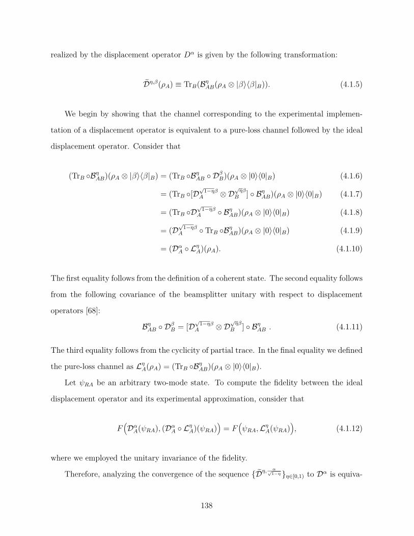
realized by the displacement operator D

α is given by the following transformation:

D

η ,β( ρA) ≡ Tr B( B

η

AB( ρA

⊗ | β ⟩⟨ β |B)) .

(4.1.5)

We begin by showing that the channel corresponding to the experimental implemen-

tation of a displacement operator is equivalent to a pure-loss channel followed by the ideal

displacement operator. Consider that

(Tr B

B

η

AB)( ρA

⊗ | β ⟩⟨ β |B) = (TrB

B

η

AB

D

β

B)( ρA

⊗ | 0 ⟩⟨ 0 |B) (4.1.6)

= (TrB

[ D

√

1 − η β

A

⊗ D

√

η β

B

] B

η

AB)( ρA

⊗ | 0 ⟩⟨ 0 |B) (4.1.7)

= (TrB

D

√

1 − η β

A

B

η

AB)( ρA

⊗ | 0 ⟩⟨ 0 |B) (4.1.8)

= ( D

√

1 − η β

A

Tr B

B

η

AB)( ρA

⊗ | 0 ⟩⟨ 0 |B) (4.1.9)

= ( D

α

A

Lη

A)( ρA) . (4.1.10)

The first equality follows from the definition of a coherent state. The second equality follows

from the following covariance of the beamsplitter unitary with respect to displacement

operators [68]:

B

η

AB

D

β

B

= [ D

√

1 − η β

A

⊗ D

√

η β

B

] B

η

AB

.

(4.1.11)

The third equality follows from the cyclicity of partial trace. In the final equality we defined

the pure-loss channel as Lη

A( ρA) = (TrB

B

η

AB)( ρA

⊗ | 0 ⟩⟨ 0 |B) .

Let ψR A

be an arbitrary two-mode state. To compute the fidelity between the ideal

displacement operator and its experimental approximation, consider that

F

(

D

α

A( ψR A) , ( D

α

A

Lη

A)( ψR A)

)

= F

(

ψR A

, Lη

A( ψR A)

)

,

(4.1.12)

where we employed the unitary invariance of the fidelity.

Therefore, analyzing the convergence of the sequence D

η ,

α

√

1 − η η ∈ [0 , 1)

to D

α is equiva-

138

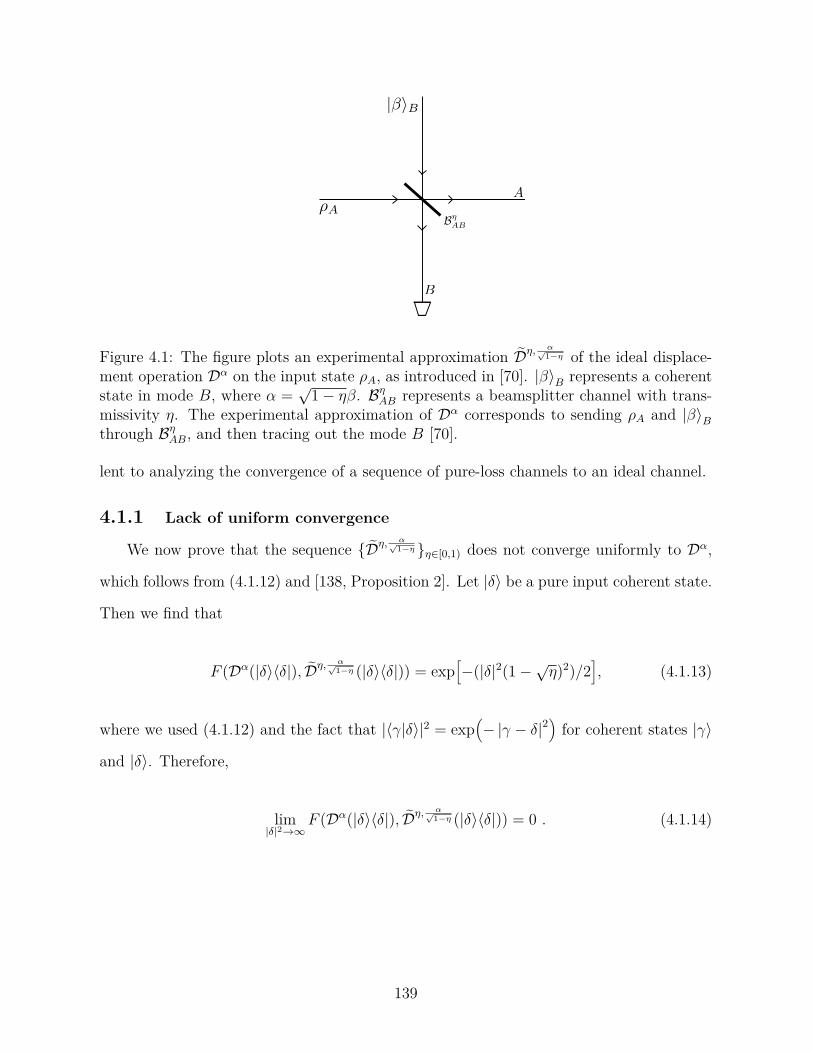
Figure 4.1: The figure plots an experimental approximation D

η ,

α

√

1 − η of the ideal displace-

ment operation D

α on the input state ρA, as introduced in [70]. | β ⟩B

represents a coherent

state in mode B , where α =

√

1 − η β . B

η

AB

represents a beamsplitter channel with trans-

missivity η . The experimental approximation of D

α corresponds to sending ρA

and | β ⟩B

through B

η

AB, and then tracing out the mode B [70].

lent to analyzing the convergence of a sequence of pure-loss channels to an ideal channel.

4.1.1 Lack of uniform convergence

We now prove that the sequence D

η ,

α

√

1 − η η ∈ [0 , 1)

does not converge uniformly to D

α,

which follows from (4.1.12) and [138, Proposition 2]. Let | δ ⟩ be a pure input coherent state.

Then we find that

F ( D

α( | δ ⟩⟨ δ | ) , D

η ,

α

√

1 − η ( | δ ⟩⟨ δ | )) = exp

[

− ( | δ |2(1 −

√

η )2) / 2

]

, (4.1.13)

where we used (4.1.12) and the fact that |⟨ γ | δ ⟩|2 = exp

(

− | γ − δ |2

)

for coherent states | γ ⟩

and | δ ⟩ . Therefore,

lim

| δ |2 →∞

F ( D

α( | δ ⟩⟨ δ | ) , D

η ,

α

√

1 − η ( | δ ⟩⟨ δ | )) = 0 . (4.1.14)

139

Let | ϕ ⟩R A

= | 0 ⟩R

| δ ⟩A. Using (2.4.12), (4.1.14), and the fact that

∥ ρ ⊗ ω − σ ⊗ ω ∥1

= ∥ ρ − σ ∥1

, (4.1.15)

for density operators ρ, σ, ω , we find that

lim

| δ |2 →∞

∥∥∥∥IR

⊗ D

α

A( ϕR A) − IR

⊗ D

η ,

α

√

1 − η

A

( ϕR A)

∥∥∥∥1

= 2 , (4.1.16)

which is the maximum value of the diamond distance between any two quantum channels.

Therefore, the definition in (2.5.1) and the equality in (4.1.16) imply that the sequence

D

η ,

α

√

1 − η η ∈ [0 , 1)

does not converge uniformly to the ideal displacement channel D

α. The

equality in (4.1.16) indicates that the ideal displacement D

α and its experimental approx-

imation D

η ,

α

√

1 − η become perfectly distinguishable in the limit that the input state has

unbounded energy. We note that the lack of uniform convergence of a sequence of pure-loss

channels to another pure-loss channel was recently studied in [138, Proposition 2].

4.1.2 Strong convergence

We now argue that the sequence D

η ,

α

√

1 − η η ∈ [0 , 1)

converges to D

α in the strong sense.

Let χρA( x, p ) denote the Wigner characteristic function [68] for the input state ρA. Let ˜ ρout

A

denote the state after the action of D

η ,

α

√

1 − η on ρA:

˜ ρout

A

= D

η ,

α

√

1 − η ( ρA) .

(4.1.17)

We now find the X , Y matrices and the d vector corresponding to the Gaussian channel

140

D

η ,

α

√

1 − η . By using (4.1.10), we get

X = diag (√

η ,

√

η ) , (4.1.18)

Y = diag (1 − η , 1 − η ) , (4.1.19)

d = (

√

2 Re ( α ) ,

√

2 Im ( α ))T . (4.1.20)

Then using (2.3.63), the characteristic function of ˜ ρout

A

is given by

χ˜ ρout

A

( x, p ) = χρA(√

η x,

√

η p ) e[ i√

2( p Re ( α ) − x Im ( α )) − (1 / 4)( x2+ p2)(1 − η )] . (4.1.21)

Moreover, the characteristic function after the action of an ideal displacement channel D

α

on ρA

is given by

χD

α( ρA)( x, p ) = χρA( x, p ) e[ i

√

2( p Re ( α ) − x Im ( α ))] .

(4.1.22)

Therefore, for each ρA

∈ D ( HA) , and for all x, p ∈ R

limη → 1

χ˜ ρout

A

( x, p ) = χD

α( ρA)( x, p ) . (4.1.23)

We have thus shown that the sequence of characteristic functions χ˜ ρout

A

converges pointwise

to χD

α( ρA), which implies by [141, Lemma 8] that the sequence D

η ,

α

√

1 − η η ∈ [0 , 1)

converges

to D

α in the strong sense.

4.1.3 Convergence in the energy-constrained diamond norm

We now discuss uniform convergence of the sequence D

η ,

α

√

1 − η η ∈ [0 , 1)

to D

α on the

set of density operators whose marginals on the channel input have bounded energy. As

observed in [137], a sequence of quantum channels converges strongly to a quantum channel

if and only if it converges uniformly on the set of density operators whose marginals on

the channel input have bounded energy. Therefore, the sequence D

η ,

α

√

1 − η η ∈ [0 , 1)

converges

141

uniformly to D

α if the input states have a finite energy constraint.

However, from an experimental perspective, it is important to know how the energy-

constrained uniform convergence depends on experimental parameters. Using (2.4.12) and

(4.1.12), we find that

1

2

∥∥∥ D

α − D

η ,

α

√

1 − η

∥∥∥⋄ E

≤ sup

ψR A:Tr( HA

ψA) ≤ E

√

1 − F [ ψR A

, Lη

A( ψR A)] (4.1.24)

=

√

1 −

[

(1 − E )√

η

⌊ E ⌋ + E √

η

⌈ E ⌉

]2

, (4.1.25)

where E = E − ⌊ E ⌋ . The equality follows from the recent result of [186] (see also

the earlier result in [180]), where the energy-constrained Bures distance [139] between two

pure-loss channels was calculated. From (4.1.25), it is easy to see that

limη → 1

1

2

∥∥∥ D

α − D

η ,

α

√

1 − η

∥∥∥⋄ E

= 0 , (4.1.26)

which justifies the energy-constrained uniform convergence of D

η ,

α

√

1 − η η ∈ [0 , 1)

to D

α. Fur-

thermore, an optimal state ψR A

that saturates the equality in (4.1.25) is

| ψ ⟩R A

=

√

1 − E |⌊ E ⌋⟩A

| τ ⟩R

+

√

E |⌈ E ⌉⟩A

∣∣∣ τ

⊥

⟩

R

, (4.1.27)

which follows directly from [186]. Here | τ ⟩ and

∣∣∣ τ

⊥

⟩

are normalized orthogonal states.

Numerical results . Next, we perform numerical evaluations to see how close the exper-

imental approximation D

η ,

α

√

1 − η is to the ideal displacement channel D

α. We denote the

energy-constrained sine distance [93, Section 12] obtained in (4.1.25) as

f ( η , E ) =

√

1 −

[

(1 − E )√

η

⌊ E ⌋ + E √

η

⌈ E ⌉

]2

. (4.1.28)

In Figure 4.2, we plot f ( η , E ) versus η for certain values of the energy constraint E .

In particular, we find that for all values of E , the experimental approximation D

η ,

α

√

1 − η

142

Figure 4.2: The figure plots the energy-constrained sine distance f ( η , E ) (4.1.28) between

an ideal displacement channel D

α and its experimental approximation D

η ,

α

√

1 − η . In the

figure, we select certain values of the energy constraint E , with the choices indicated next

to the figure. In all the cases, D

η ,

α

√

1 − η simulates D

α with a high accuracy for values of

η ≈ 1 . Moreover, for a fixed value of η , the simulation of D

α is more accurate for low

values of the energy constraint on input states.

simulates the ideal displacement D

α with a high accuracy for η ≈ 1 . Moreover, for a fixed

value of η , the simulation of D

α is more accurate for low values of the energy constraint on

input states.

In Figure 4.3, we zoom in on Figure 4.2 for high values of η . Figure 4.3 indicates that

it is only for low values of E and high values of η that high accuracy in simulating D

α

can be achieved. Therefore, energy constraints on the input states play a critical role in

simulating ideal unitary operations and determining error propagation.

We now analyze a simple case when the energy constraint E on the input density

operators takes on an integer value. From (4.1.25), we find that

inf

ψR A:Tr( HA

ψA) ≤ E

F [ D

α( ψR A) , D

η ,

α

√

1 − η ( ψR A)] = η

E .

(4.1.29)

Therefore, for a given energy constraint on the input states, and to implement an ideal

displacement channel D

α with any desired accuracy, one can find η from (4.1.25)–(4.1.29),

and the corresponding β from

√

1 − η β = α . The equality in (4.1.29) illustrates just how

difficult it is to achieve a good accuracy in simulating an ideal displacement channel: in

143

Figure 4.3: The figure plots Figure 4.2 for high values of η . The figure indicates that, only

for low values of E and high values of η , high accuracy in simulating D

α can be achieved.

order to achieve the same fidelity, one requires an exponential increase in η to match only

a linear increase in E .

We now summarize the results from Sections 4.1.1–4.1.3. From Sections 4.1.1 and 4.1.2,

it follows that the sequence D

η ,

α

√

1 − η η ∈ [0 , 1)

does not converge uniformly to D

α. Rather,

convergence occurs in the strong sense. In other words, convergence of D

η ,

α

√

1 − η η ∈ [0 , 1)

to

D

α is not independent of the input state; i.e., there exists an input state for which the

experimental implementation of a displacement operation has the maximum possible value

of the worst-case error.

It is important to stress that, although for a fixed finite value of the energy-constraint

parameter E the limit η → 1 is necessary for the implementation of a displacement

operation D

α using D

η ,

α

√

1 − η η ∈ [0 , 1)

with a high accuracy, it also relies on the fact that

√

1 − η β = α . Due to the unitary invariance of the fidelity as shown in (4.1.12), the fidelity

between D

α and D

η ,

α

√

1 − η η ∈ [0 , 1)

becomes independent of the parameter β . However, it is

implicit from

√

1 − η β = α that η → 1 requires β → ∞ . Although high values of β are

experimentally achievable, the ideal displacement operation is achieved only in the limiting

sense. This raises a further question: is it possible to implement an ideal displacement

operation through a different procedure than in [70], such that a high accuracy can be

achieved?

144

4.1.4 Convergence for a tensor product of displacements

Let us briefly discuss the various notions of convergence for experimental approxima-

tions of a tensor product of ideal displacement channels. Let D

αi L

i =1

be a set of L different

displacement channels. We approximate the tensor product of these operators by a ten-

sor product of D

ηi

,βi L

i =1, such that

√

1 − ηi

βi

= αi, for i ∈ 1 , . . . , L . From the same

counterexample given above (coherent states with large energy), it follows directly that the

sequence ⊗L

i =1

D

ηi

,αi

/√

1 − ηi η1

,...,ηL

∈ [0 , 1)

does not converge uniformly to

⊗L

i =1

D

αi . Rather,

the convergence holds in the strong sense, as a consequence of [117, Proposition 1]. More-

over, suppose that there is an average energy constraint on the input state to the tensor

product of displacement operators, i.e., Tr

(

HAL ψAL

)

≤ E , where

HAL ≡ HA

⊗ I ⊗ · · · ⊗ I + · · · + I ⊗ · · · ⊗ I ⊗ HA

,

(4.1.30)

and E ∈ [0 , ∞ ) . Let Tr( HA

ψAi) = Ei, where Ei

∈ [0 , ∞ ) , ∀ i ∈ 1 , . . . , L .


1

2

∥∥∥∥∥

(

K⊗

i =1

D

αi

)

( ψR AK ) −

(

K⊗

i =1

D

ηi

,αi

/√

1 − ηi

)

( ψR AK )

∥∥∥∥∥

1

≤

K∑

i =1

C

(

Lηi

Ai( ψR Ai

) , IAi( ψR Ai

)

)

(4.1.31)

≤ max

Ei

i:∑

i

Ei

≤ E

K∑

i =1

√

1 − [(1 − Ei

)√

ηi

⌊ Ei

⌋ + Ei

√

ηi

⌈ Ei

⌉]2 . (4.1.32)

The first inequality follows from (2.4.12) and [117, Proposition 1]. The last inequality

follows from the recent result of [190], and due to the maximization over a set of energy

values satisfying the input energy constraint. Since the chain of inequalities is true for all

145

input states satisfying the input energy constraint, the following holds

1

2

∥∥∥∥∥

K⊗

i =1

D

αi −

K⊗

i =1

D

ηi

,αi

/√

1 − ηi

∥∥∥∥∥

⋄ E

≤ max

Ei

i:∑

i

Ei

≤ E

K∑

i =1

√

1 − [(1 − Ei

)√

ηi

⌊ Ei

⌋ + Ei

√

ηi

⌈ Ei

⌉]2 . (4.1.33)

Therefore, ⊗K

i =1

D

ηi

,αi

/√

1 − ηi η1

,...,ηK

∈ [0 , 1)

converges uniformly to

⊗K

i =1

D

αi on the set of

density operators whose marginals on the channel input have bounded energy.

4.1.5 Estimates of energy-constrained diamond distance

We now provide good estimates of the energy-constrained diamond distance, as defined

in (2.4.17) between the ideal displacement operation D

α and its experimental approximation

D

η ,α/√

1 − η. In particular, we introduce two different techniques to lower bound the energy-

constrained diamond distance.

A first technique is based on the trace distance between IR

⊗ D

α( ψR A) and IR

⊗

D

η ,α/√

1 − η( ψR A) for a finite energy-constraint E , i.e., Tr(ˆ nψA) ≤ E , where ψR A

is given by

(4.1.27). Since the energy-constrained diamond distance, as defined in (2.4.17), involves an

optimization over all input states satisfying the energy constraint, we find that

∥∥∥ IR

⊗ D

α( ψR A) − IR

⊗ D

η ,

α

√

1 − η ( ψR A)

∥∥∥1

≤

∥∥∥ D

α − D

η ,

α

√

1 − η

∥∥∥⋄ E

.

(4.1.34)

A second technique is based on the numerical evaluation of the energy-constrained

diamond distance between D

α and D

η ,α/√

1 − η on a truncated Hilbert space. In particular,

we consider input states to these quantum channels such that instead of acting on an

infinite-dimensional separable Hilbert space, these states act on an ( M + 1) -dimensional

Fock space. Moreover, we consider a mean photon number constraint on these states. Let

HM

denote an ( M + 1) -dimensional Fock space. Let ˆ n

denote the following truncated

146

number operator:

ˆ n

=

M∑

n =0

n | n ⟩⟨ n | .

(4.1.35)

Let φA

∈ D ( HM) . Then the following inequality holds:

Tr(ˆ n

φA) ≤ E ,

(4.1.36)

where E denotes the mean energy constraint.

We define the energy-constrained diamond distance between two quantum channels

NA → B

and MA → B

on a truncated Hilbert space as

∥NA → B

− MA → B

∥⋄ E ,M

≡ sup

ϕR A

∈D ( H

⊗ 2

M

):Tr(ˆ n

ϕA) ≤ E

∥NA → B( ϕR A) − MA → B( ϕR A) ∥1

,

(4.1.37)

where E and M denote the mean energy constraint and the truncation parameter, respec-

tively, and ϕR A

= | ϕ ⟩⟨ ϕ |R A

is a purification of the state ϕA. Moreover, it is implicit that the

identity channel acts on the reference system R . Finally, note that the following identity

holds:

∥NA → B

− MA → B

∥⋄ E ,M

= sup

ϕR A

∈D ( H

⊗ 2

M

):Tr(ˆ nϕA) ≤ E

∥NA → B( ϕR A) − MA → B( ϕR A) ∥1

,

(4.1.38)

where we have replaced ˆ n

with ˆ n , following as a consequence of the reduced state of

ϕR A

∈ D ( H

⊗ 2

M

) on A having support only on the truncated space and from the Schmidt

decomposition, implying that the reference system R need only have support as large as

the input space A .

We now show that the set of density operators acting on a truncated Hilbert space

with a finite mean energy constraint (yet an arbitrarily high truncation parameter) is

dense in the set of density operators acting on an infinite-dimensional Hilbert space and

with the same mean energy constraint. In other words, any finite mean energy state acting

on an infinite-dimensional separable Hilbert space can be approximated with an arbitrary

147

accuracy by a state with the same finite mean energy acting on a truncated Hilbert space

with a sufficiently high value of the truncation parameter. Let ρR A

denote a density operator

acting on an infinite-dimensional separable Hilbert space, such that Tr(ˆ nA

ρR A) ≤ E , where

E > 0 . Let ΠM

A

denote an M -dimensional projector defined as

ΠM

A

=

M∑

n =0

| n ⟩⟨ n | .

(4.1.39)


Tr

(

ΠM

A

ρR A

)

= Tr( ρR A) −

∞∑

n = M +1

⟨ n | ρA

| n ⟩ (4.1.40)

≥ 1 −

∞∑

n = M +1

n

M + 1

⟨ n | ρA

| n ⟩ (4.1.41)

≥ 1 −

1

M + 1

( ∞∑

n =0

n ⟨ n | ρA

| n ⟩

)

(4.1.42)

≥ 1 −

E

M + 1

. (4.1.43)

The first inequality follows from the fact that n/ ( M + 1) ≥ 1 for all n ∈ [ M + 1 , ∞ ) . The

second inequality follows because

∑M

n =0

n ⟨ n | ρA

| n ⟩ is a sum of positive numbers. The last

inequality follows because Tr(ˆ nA

ρA) ≤ E . We note that (4.1.43) can also be derived from

the Fock cutoff lemma in [191].

Let ρM

R A

denote the following truncated state

ρM

R A

=

ΠM

A

ρR AΠM

A

Tr(ΠM

A

ρR A)

.

(4.1.44)

The following proposition establishes a bound on the trace distance between ρR A

and ρM

R A.

Proposition 115 Let ρR A

be a density operator acting on an infinite-dimensional separable

Hilbert space such that Tr(ˆ nA

ρR A) ≤ E , where E > 0 , and ˆ nA

is the number operator as

defined in (2.3.4) . Let ρM

R A

be the M -dimensional truncation of the state ρR A, as defined in

148

(4.1.44) . Then

1

2

∥∥∥ ρR A

− ρM

R A

∥∥∥1

≤

√

E

M + 1

.

(4.1.45)

Proof. The proof follows directly from (4.1.43) and the gentle measurement lemma intro-

duced in [192] and subsequently improved in [193].

Proposition 116 below states that for low values of the mean energy constraint E ,

the energy-constrained diamond distance between two quantum channels N and M can

be estimated with an arbitrarily high accuracy by using the energy-constrained diamond

distance on a truncated input Hilbert space with sufficiently high values of the truncation

parameter M .

Proposition 116 Let N and M be quantum channels, and let E be the energy constraint

on the input states to these channels. Let M denote the truncation parameter. Then

1

2

∥N − M∥⋄ E ,M

≤

1

2

∥N − M∥⋄ E

≤

1

2

∥N − M∥⋄ E ,M

+ 2

√

E

M + 1

.

(4.1.46)

Proof. The inequality ∥N − M∥⋄ E ,M

≤ ∥N − M∥⋄ E

follows from (2.4.17) and (4.1.38).

We now prove the other inequality. Let ρR A

be a density operator acting on an

infinite-dimensional separable Hilbert space such that Tr(ˆ nA

ρR A) ≤ E . Let ρM

R A

be the

M -dimensional truncation of the state ρR A

as defined in (4.1.44). Consider the following

chain of inequalities:

∥N ( ρR A) − M ( ρR A) ∥1

≤

∥∥∥ N ( ρR A) − N ( ρM

R A)

∥∥∥1

+

∥∥∥ N ( ρM

R A) − M ( ρM

R A)

∥∥∥1

+

∥∥∥ M ( ρM

R A) − M ( ρR A)

∥∥∥1

(4.1.47)

≤ 2

∥∥∥ ρR A

− ρM

R A

∥∥∥1

+

∥∥∥ N ( ρM

R A) − M ( ρM

R A)

∥∥∥1

(4.1.48)

≤ 4

√

E

M + 1

+ ∥N − M∥⋄ E ,M

. (4.1.49)

In all the steps above, it is implicit that the identity channel acts on the reference system

149

R . The first inequality is the consequence of triangle inequality for the trace distance.

The second inequality follows from monotonicity of the trace distance. The last inequality

follows from Proposition 115 and from (4.1.37). Since the chain of inequalities holds for all

input states ρR A

satisfying the energy constraint, the desired result follows.

We now study the aforementioned two techniques in detail to characterize the perfor-

mance of the simulation of an ideal displacement operator. It is evident from Figure 4.2

that for a fixed value of η , the accuracy in simulating an ideal displacement operation D

α

by using the protocol from [70] is reasonable only for low values of the energy constraint

on input states. Therefore, we now study the simulation of D

α in detail only for low values

of the energy constraint.

Let 0 < E < 1 . Then

1

2

∥∥∥ IR

⊗ D

α( ψR A) − IR

⊗ D

η ,

α

√

1 − η ( ψR A)

∥∥∥1

=

1

2[ E (1 − η ) + (1 −

√

η ) κ ( η , E )] (4.1.50)

≡ d1( η , E ) , (4.1.51)

where

κ ( η , E ) =

√

E (4 + E ( η + 2√

η − 3)) ,

(4.1.52)

E = E − ⌊ E ⌋ , and ψR A

is given by (4.1.27).

Therefore, from (4.1.34), it follows that (4.1.50) is a lower bound on the energy-

constrained diamond distance between D

α and D

η ,α/√

1 − η for 0 < E < 1 , i.e.,

d1( η , E ) ≤

1

2

∥∥∥ D

α − D

η ,

α

√

1 − η

∥∥∥⋄ E

.

(4.1.53)

We now provide a proof for (4.1.50). Let t =

√

η and r =

√

1 − η . Then the action of

a pure-loss channel with transmissivity η on ψR A

in (4.1.27) is given by

( IR

⊗ Lη

A)( ψR A) = Tr B(( IR

⊗ B

η

AB)( ψR A

⊗ | 0 ⟩⟨ 0 |B)) ≡ ρR A

. (4.1.54)

150

Consider the following unitary evolution of the pure state | ψ ⟩R A

⊗ | 0 ⟩B:

( IR

⊗ B

η

AB)( | ψ ⟩R A

⊗ | 0 ⟩B)

= B

η

AB(

√√√√

1 − E

⌊ E ⌋ !

(ˆ a†

in)⌊ E ⌋ | 0 ⟩A

| τ ⟩R

| 0 ⟩B

+

√√√√

E

⌈ E ⌉ ! (ˆ a†

in)⌈ E ⌉ | 0 ⟩A

∣∣∣ τ

⊥

⟩

R

| 0 ⟩B) (4.1.55)

=

√√√√

1 − E

⌊ E ⌋ !

( t ˆ a†

out

+ rb†

out)⌊ E ⌋ | 0 ⟩A

| τ ⟩R

| 0 ⟩B

+

√√√√

E

⌈ E ⌉ ! ( t ˆ a†

out

+ rb†

out)⌈ E ⌉ | 0 ⟩A

∣∣∣ τ

⊥

⟩

R

| 0 ⟩B

(4.1.56)

=

√

1 − E

∑

k1

√√√√

(⌊ E ⌋

k1

)

tk1 r

⌊ E ⌋− k1 | k1

⟩A

| τ ⟩R

|⌊ E ⌋ − k1

⟩B

+

√

E

∑

k2

√√√√

(⌈ E ⌉

k2

)

tk2 r

⌈ E ⌉− k2 | k2

⟩A

∣∣∣ τ

⊥

⟩

R

|⌈ E ⌉ − k2

⟩B

. (4.1.57)

The second equality follows from the beamsplitter transformation in the Heisenberg picture

(2.3.78). Then the density operator after tracing out B in (4.1.56) is given by

ρR A

= (1 − E )

∑

k1

(⌊ E ⌋

k1

)

t2 k1 r2( ⌊ E ⌋− k1) | k1

⟩⟨ k1

|A

| τ ⟩⟨ τ |R

+ E

∑

k2

(⌈ E ⌉

k2

)

t2 k2 r2( ⌈ E ⌉− k2) | k2

⟩⟨ k2

|A

| τ

⊥ ⟩⟨ τ

⊥ |R

+

√

(1 − E ) E

∑

k1

√√√√

(⌊ E ⌋

k1

)(

⌈ E ⌉

k1

+ 1

)

t(2 k1+1) r

⌊ E ⌋ + ⌈ E ⌉− 2 k1

− 1

×

| k1

⟩⟨ k1

+ 1 |A

| τ ⟩⟨ τ

⊥ |R

+ | k1

+ 1 ⟩⟨ k1

|A

| τ

⊥ ⟩⟨ τ |R

.

(4.1.58)

On the other hand, the density operator of the state in (4.1.27) is given by

ψR A

= (1 − E ) |⌊ E ⌋⟩⟨⌊ E ⌋|A

| τ ⟩⟨ τ |R

+ E |⌈ E ⌉⟩⟨⌈ E ⌉|A

| τ

⊥ ⟩⟨ τ

⊥ |R

+

√

(1 − E ) E

(

|⌊ E ⌋⟩⟨⌈ E ⌉|A

| τ ⟩⟨ τ

⊥ |R

+ |⌈ E ⌉⟩⟨⌊ E ⌋|| τ

⊥ ⟩⟨ τ |R

)

. (4.1.59)

151

Let ωR A

denote the operator corresponding to the difference of ρR A

in (4.1.58) and ψR A

in (4.1.59).

ωR A

= ρR A

− ψR A

(4.1.60)

= (1 − E )

∑

k1

(⌊ E ⌋

k1

)

t2 k1 r2( ⌊ E ⌋− k1) | k1

⟩⟨ k1

|A

− |⌊ E ⌋⟩⟨⌊ E ⌋|A

| τ ⟩⟨ τ |R

+ E

∑

k2

(⌈ E ⌉

k2

)

t2 k2 r2( ⌈ E ⌉− k2) | k2

⟩⟨ k2

|A

− |⌈ E ⌉⟩⟨⌈ E ⌉|A

| τ

⊥ ⟩⟨ τ

⊥ |R

+

√

(1 − E ) E

∑

k1

√√√√

(⌊ E ⌋

k1

)(

⌈ E ⌉

k1

+ 1

)

t(2 k1+1) r

⌊ E ⌋ + ⌈ E ⌉− 2 k1

− 1

×

| k1

⟩⟨ k1

+ 1 |A

| τ ⟩⟨ τ

⊥ |R

+ | k1

+ 1 ⟩⟨ k1

|A

| τ

⊥ ⟩⟨ τ |R

− |⌊ E ⌋⟩⟨⌈ E ⌉|A

| τ ⟩⟨ τ

⊥ |R

− |⌈ E ⌉⟩⟨⌊ E ⌋|| τ

⊥ ⟩⟨ τ |R

. (4.1.61)

We now find ∥ ωR A

∥1

for a simple case. Let 0 < E < 1 . Then ⌊ E ⌋ = 0 and ⌈ E ⌉ = 1 .

Let | τ ⟩ = | 0 ⟩ and

∣∣∣ τ

⊥

⟩

= | 1 ⟩ . Therefore, the operator ωR A

is given by

ωR A

= E

r2 | 0 ⟩⟨ 0 |A

+ t2 | 1 ⟩⟨ 1 |A

− | 1 ⟩⟨ 1 |A

| 1 ⟩⟨ 1 |R

+

√

(1 − E ) E

( t − 1)

(

| 0 ⟩⟨ 1 |A

⊗ | 0 ⟩⟨ 1 |R

+ | 1 ⟩⟨ 0 |A

⊗ | 1 ⟩⟨ 0 |R

) . (4.1.62)

152

After expressing r and t in terms of η , the matrix representation of ωR A

is as follows

ωR A

=

0 0 0 −

√

(1 − E ) E (1 −

√

η )

0 E (1 − η ) 0 0

0 0 0 0

−

√

(1 − E ) E (1 −

√

η ) 0 0 − E (1 − η )

(4.1.63)

Then ∥ ωR A

∥1

is given by [164]

1

2

∥ ωR A

∥1

=

1

2

E (1 − η ) +

1

2

∣∣∣∣∣∣(√

η − 1)

E (1 +

√

η ) −

√√√√

E

[

4 + E ( − 3 + 2√

η + η )

]

∣∣∣∣∣∣

+

1

2

∣∣∣∣∣∣(√

η − 1)

E (1 +

√

η ) +

√√√√

E

[

4 + E ( − 3 + 2√

η + η )

]

∣∣∣∣∣∣

.

(4.1.64)

Since

E (1 +

√

η ) ≤

√√√√

E

[

4 + E ( − 3 + 2√

η + η )

]

(4.1.65)

for all 0 < E < 1 and η ≥ 0 , we get that

1

2

∥ ωR A

∥1

=

1

2

E (1 − η ) + (1 −

√

η )

√√√√

E

[

4 + E ( − 3 + 2√

η + η )

] .

(4.1.66)

A second method to obtain a lower bound on the energy-constrained diamond distance

between two quantum channels NA → B

and MA → B

is to truncate the infinite-dimensional

separable Hilbert space to a finite-dimensional Hilbert space and apply energy constraints

on channel input states according to the truncated number operator, as defined in (4.1.35)–

(4.1.36). In particular, we obtain the energy-constrained diamond distance between NA → B

and MA → B

on a truncated Hilbert space by using a semi-definite program (SDP) from [138],

which is inspired from an SDP defined in the context of finite-dimensional quantum chan-

nels in [187, 188]. We use the following SDP to estimate the energy-constrained diamond

153

distance between two quantum channels NA → B

and MA → B:

∥N − M∥⋄ E ,M

=

sup Tr( WR B

JR B)

subject to 0 ≤ WR B

≤ ρR

⊗ IB

,

Tr( ρR) = 1 , ρR

≥ 0 ,

Tr(ˆ n

ρR) ≤ E ,

(4.1.67)

where M is the truncation parameter, E is the mean energy-constraint parameter, and ˆ n

is given by (4.1.35). Moreover, JR B

denotes the operator corresponding to the difference

of the Choi operators of quantum channels N and M on the truncated Hilbert space HM

and is defined as follows

JR B

= ( IR

⊗ NA → B)(ΓR A) − ( IR

⊗ MA → B)(ΓR A) ,

(4.1.68)

where ΓR A

= | Γ ⟩⟨ Γ |R A

is the projection onto the unnormalized maximally entangled vector

on the truncated Hilbert space HM , i.e.,

| Γ ⟩R A

=

M∑

n =0

| n ⟩R

| n ⟩A

.

(4.1.69)

For a small value of the energy-constraint parameter E , the truncation parameter

M can be chosen such that the value of ∥N − M∥⋄ E ,M

does not change significantly by

increasing M further. For example, in the context of the ideal displacement operation D

α

and its experimental approximation D

η ,α/√

1 − η, we find that for E ≪ 1 , the truncation

parameter M = 6 provides a good estimate of

∥∥∥ D

α − D

η ,

α

√

1 − η

∥∥∥⋄ E

. For E ≪ 1 , we define

d2( η , E ) ≡

1

2

∥∥∥ D

α − D

η ,

α

√

1 − η

∥∥∥⋄ E ,M

,

(4.1.70)

154

0.2 0.4 0.6 0.8 1.0

0.05

0.10

0.15

0.20

0.25

0.30

0.35

Figure 4.4: The figure depicts the lower bound d1( η , E ) in (4.1.50), the lower bound d2( η , E )

in (4.1.70), and the upper bound f ( η , E ) in (4.1.28) for the fixed value E = 0 . 06 . Here,

d1( η , E ) is the trace distance between the outputs of an ideal displacement D

α( ψR A) and

its experimental approximation D

η ,α/√

1 − η( ψR A) , when the input state ψR A

is such that it

optimizes the energy-constrained sine distance between D

α and D

η ,α/√

1 − η and is given by

(4.1.27). Moreover, d2( η , E ) is the energy-constrained diamond distance between D

α and

D

η ,α/√

1 − η on a truncated Hilbert space with the truncation parameter M = 6 , and f ( η , E )

is the energy-constrained sine distance between D

α and D

η ,α/√

1 − η. For low values of η ,

d1( η , E ) is close to d2( η , E ) . The figure indicates that for a fixed value of E , high accuracy

in simulating D

α can be achieved only for high values of η .

for M = 6 . From Proposition 116 it follows that

d2( η , E ) ≤

1

2

∥∥∥ D

α − D

η ,

α

√

1 − η

∥∥∥⋄ E

.

(4.1.71)

Let us study in detail the case when the input states have mean energy constraint

E = 0 . 06 . We first calculate d1( η , E ) by using (4.1.50) and then find d2( η , E ) , as defined

in (4.1.70) by solving the corresponding SDP in (4.1.67) [164]. We then compare both

d1( η , E ) and d2( η , E ) with the energy-constrained sine distance f ( η , E ) between D

α and

D

η ,α/√

1 − η, as calculated in (4.1.28).

In Figure 4.4, we plot the lower bound d1( η , E ) in (4.1.50), the lower bound d2( η , E ) in

(4.1.70), and the upper bound f ( η , E ) in (4.1.28) versus η for E = 0 . 06 . In particular, we

find that d1( η , E ) overlaps with d2( η , E ) for small values of η . From numerical evaluations,

we find that the value of d2( η , E ) does not change significantly with a further increment

in M ≥ 6 . These findings indicate that d2( η , E ) is a good lower bound on the energy-

155

constrained diamond distance between D

α and D

η ,α/√

1 − η, and furthermore, that the upper

bound in Proposition 116 is loose for this case. Moreover, from Figure 4.4, it is evident that

d1( η , E ) is also a tight lower bound. Although there is a significant gap between f ( η , E )

and d2( η , E ) in Figure 4.4, the key message of our results remains the same; i.e., in order

to achieve a high accuracy in simulating an ideal displacement operation D

α by using the

protocol from [70], the value of η should be very high and the mean energy of the input

states should be very low. In summary, a good estimation of the accuracy in simulating an

ideal displacement operation can be obtained from the following three methods:

1. The energy-constrained sine distance between D

α and D

η ,α/√

1 − η can be calculated

from the analytical expression obtained in (4.1.28).

2. A lower bound on the energy-constrained diamond distance between D

α and D

η ,α/√

1 − η

can be established by solving an SDP in (4.1.67) on a truncated Hilbert space [164] .

3. For a fixed energy range ⌊ E ⌋ ≤ E ≤ ⌈ E ⌉ , a lower bound on the energy-constrained

diamond distance between D

α and D

η ,α/√

1 − η can be established by finding the trace

distance between IR

⊗ D

α( ψR A) and IR

⊗ D

η ,α/√

1 − η( ψR A) , where ψR A

is given by

(4.1.27). In particular, for 0 < E < 1 , an analytical expression for the trace distance


4.2 Approximation of a Beamsplitter

In this section, we analyze convergence of the experimental implementations of a beam-

splitter transformation.

Let ρA1

A2

be a two-mode input quantum state, and let B

η ,ϕ denote the beamsplitter

transformation of transmissivity η ∈ (0 , 1) and phase ϕ ∈ [0 , 2 π ] acting on mode A1

and

A2, i.e.,

B

η ,ϕ( ρA1

A2) = U

θ ,ϕ

BS

( ρA1

A2)( U

θ ,ϕ

BS

)† ,

(4.2.1)

where η = (cos θ )2.

156

There are at least two different ways to model the noise in implementing B

η ,ϕ. A

first method consists of an ideal beamsplitter preceded and followed by a tensor product

of pure-loss channels with transmissivity η

′. We denote the channel corresponding to the

experimental implementation of the beamsplitter transformation B

η ,ϕ by B

η ,ϕ,η

′ , such that

B

η ,ϕ,η

′( ρA1

A2) ≡ ( Lη

′

A1

⊗ Lη

′

A2) B

η ,ϕ ( Lη

′

A1

⊗ Lη

′

A2)( ρA1

A2) .

(4.2.2)

This models the physical process when there is a non-zero probability of absorption of the

radiation, along with reflection and transmission. We note that the beam splitter channel

with transmissivity η and the channel corresponding to a tensor product of two pure-loss

channels with equal transmissivity η

′ commute, i.e.,

( Lη

′

A1

⊗ Lη

′

A2) B

η ,ϕ( · ) = B

η ,ϕ ( Lη

′

A1

⊗ Lη

′

A2)( · ) .

(4.2.3)

Since a concatenation of two pure-loss channels Lη1 and Lη2 is another pure-loss chan-

nel Lη1

η2 with transmissivity η1

η2, we consider the following channel as an experimental

approximation of the beamsplitter:

B

η ,ϕ,η

′( ρA1

A2) ≡ B

η ,ϕ ( Lη

′

A1

⊗ Lη

′

A2)( ρA1

A2) ,

(4.2.4)

Now let ψR A1

A2

denote an arbitrary four-mode pure state, where it is understood that

R is a two-mode system. From invariance of the fidelity under a unitary transformation,

we find that

F ( B

η ,ϕ( ψR A1

A2) , B

η ,ϕ,η

′( ψR A1

A2)) = F ( ψR A1

A2

, ( Lη

′

A1

⊗ Lη

′

A2)( ψR A1

A2)) ,

(4.2.5)

where it is implicit that the identity channel acts on the reference system R .

From arguments similar to those given in Section 4.1.1, we find that the sequence

157

B

η ,ϕ,η

′ η

′ ∈ [0 , 1)

does not converge uniformly to B

η ,ϕ. In particular, let ψA1

A2

= | δ ⟩⟨ δ |A1

⊗

| 0 ⟩⟨ 0 |A2

be a tensor product of a coherent state and a vacuum state. Then we find that

F ( B

η ,ϕ( ψA1

A2) , B

η ,ϕ,η

′( ψA1

A2)) = exp

[

− ( | δ |2(1 −

√

η

′)2) / 2

]

(4.2.6)

Therefore, from arguments similar to (4.1.14) and (4.1.16), it follows that the ideal beam-

splitter B

η ,ϕ and its experimental approximation B

η ,ϕ,η

′ become perfectly distinguishable in

the limit that the input state has unbounded energy. Hence the uniform convergence does

not hold.

We now argue that the sequence converges B

η ,ϕ,η

′ η

′ ∈ [0 , 1)

to B

η ,ϕ in the strong sense.

Let χρA1

A2( x1

, p1

, x2

, p2) denote the Wigner characteristic function for the input state ρA1

A2 .

Let ˜ ρout

A1

A2( η , ϕ, η

′) denote the state after the action of B

η ,ϕ,η

′ on ρA1

A2 :

˜ ρout

A1

A2( η , ϕ, η

′) = B

η ,ϕ,η

′( ρA1

A2) .

(4.2.7)

We now find the terms involved in (2.3.63) for both B

η ,ϕ( ρA1

A2) and ρη ,ϕ,η

′

A1

A2 . The X B

η ,ϕ,η

′

matrix corresponding to the operation B

η ,ϕ,η

′ is given by

X B

η ,ϕ,η

′

= XB

η ,ϕ ·

√

η

′ I4

,

(4.2.8)

where I4

is a four-dimensional identity matrix. Moreover, the Y B

η ,ϕ,η

′

matrix is given by

Y B

η ,ϕ,η

′

= (1 − η

′) I4

.

(4.2.9)

Let r = ( x1

, p1

, x2

, p2)T. Then, for each ρA1

A2

∈ D ( HA1

⊗ HA2) , and for all x1

, p1

, x2

, p2

∈ R

158

lim

η

′ → 1

χ˜ ρout

A1

A2( η ,ϕ,η

′)( r ) = lim

η

′ → 1

χρA1

A2(

√

η

′ΩT XT

B

η ,ϕΩ r ) exp

(

−1

4(1 − η

′) rT r

)

(4.2.10)

= χρA1

A2(ΩT XT

B

η ,ϕΩ r ) (4.2.11)

= χB

η ,ϕ( ρA1

A2 )( r ) . (4.2.12)

We have thus shown that the sequence of characteristic functions χ˜ ρout

A1

A2( η ,ϕ,η

′)

converges

pointwise to χB

η ,ϕ( ρA1

A2 ), which implies by [141, Lemma 8] that the sequence B

η ,ϕ,η

′ η

′ ∈ [0 , 1)

converges to B

η ,ϕ in the strong sense.

Similar to Section 4.1.3, we investigate the dependence of convergence of the sequence

of B

η ,ϕ,η

′ η

′ ∈ [0 , 1)

to B

η ,ϕ on the experimental parameters when there is a finite energy

constraint on the input states. Let A = A1

A2. Consider the following chain of inequalities:

1

2

∥B

η ,ϕ − B

η ,ϕ,η

′ ∥⋄ E

≤ sup

ψR A:Tr( HA

ψA) ≤ E

C ( ψR A

, ( Lη

′

A1

⊗ Lη

′

A2)( ψR A)) (4.2.13)

= f ( η

′ , E ) , (4.2.14)

where HA

= HA1

⊗ IA2

+ IA1

⊗ HA2

and f ( η

′ , E ) is given by (4.1.28). The first inequality

follows from (2.4.12). The last inequality follows from the recent result of [186], which

holds for a tensor product of loss channels with the same transmissivity. Therefore, from

the analysis in Section 4.1.3, it follows that the accuracy in implementing B

η ,ϕ using B

η ,ϕ,η

′ is

high only for high values of the loss parameter η

′ and low values of the energy constraint E .

A second experimental approximation of an ideal beamsplitter is a phenomenological

model that accounts for the imprecision in implementing B

θ ,ϕ with an exact value of the

parameters θ and ϕ , as defined in (2.3.52). For the analysis that follows, we fix ϕ = 0 ,

which is typically considered in experiments. We denote the ideal beamsplitter for ϕ = 0

by B

θ. We note that a similar analysis follows for ϕ = π / 2 .

159

The channel corresponding to an experimental approximation of B

θ is given by

B

θ ,σ ≡

∫ 2 π

0

dθ

′ p ( θ

′ , θ , σ, 0 , 2 π ) B

θ

′

,

(4.2.15)

where p ( θ

′ , θ , σ, a, b ) is a truncated normal distribution with location parameter θ , scale

parameter σ , truncation range in between a and b , and is given by

p ( θ

′ , θ , σ, a, b ) =

ϕ (( θ

′ − θ ) /σ )

σ [Φ(( b − θ ) /σ ) − Φ(( a − θ ) /σ )]

,

(4.2.16)

where

ϕ ( x ) =

1

√

2 π

exp

(

− x2 / 2

)

, (4.2.17)

Φ( x ) =

1

2(1 + erf ( x/

√

2)) , (4.2.18)

and erf ( x ) is the error function.

Now let ψA1

A2

= | α ⟩⟨ α |A1

⊗ | 0 ⟩⟨ 0 |A2

be an input state, where | α ⟩ is a coherent state.

From (4.2.15) it follows that

F ( B

θ( ψA1

A2) , B

θ ,σ( ψA1

A2)) =

∫ 2 π

0

dθ

′ p ( θ

′ , θ , σ, 0 , 2 π ) F ( B

θ( ψA1

A2) , B

θ

′( ψA1

A2)) .

(4.2.19)

Now consider that

F ( B

θ( ψA1

A2) , B

θ

′( ψA1

A2)) = F ( ψA1

A2

, B( − θ ) B

θ

′( ψA1

A2)) (4.2.20)

= exp

[

− 2 | α |2(sin( θ

′ − θ ))2

]

, (4.2.21)

which converges to zero as | α |2 → ∞ . Then from (4.2.19) and by an application of the dom-

inated convergence theorem, it follows that the sequence B

θ ,σ σ ∈ [0 , ∞ )

does not converge

uniformly to the ideal beamsplitter B

θ.

160

We now show that convergence occurs in the strong sense. Let ψR A1

A2

denote the input

state. Then the following holds:

F ( B

θ( ψR A1

A2) , B

θ ,σ( ψR A1

A2)) =

∫ 2 π

0

dθ

′ p ( θ

′ , θ , σ, 0 , 2 π ) F ( B

θ( ψR A1

A2) , B

θ

′( ψR A1

A2)) .

(4.2.22)

Since lim σ → 0

p ( θ

′ , θ , σ ) = δ ( θ − θ

′) , it follows that

limσ → 0

F ( B

θ( ψR A1

A2) , B

θ ,σ( ψR A1

A2)) = 1 ,

(4.2.23)

which implies that the sequence B

θ ,σ σ ∈ [0 , ∞ )

converges strongly to B

θ.

We now investigate convergence of the sequence B

θ ,σ σ ∈ [0 , ∞ )

to B

θ in terms of the ex-

perimental parameters when there is a finite energy constraint on the input states. Consider

the following chain of inequalities:

1

2

∥B

θ − B

θ ,σ ∥⋄ E

≤

1

2

∫ 2 π

0

dθ

′ p ( θ

′ , θ , σ, 0 , 2 π ) ∥B

θ − B

θ

′ ∥⋄ E

(4.2.24)

=

1

2

∫ 2 π

0

dθ

′ p ( θ

′ , θ , σ, 0 , 2 π ) ∥I − B

θ

′ − θ ∥⋄ E

(4.2.25)

≤

∫ 2 π

0

dθ

′ p ( θ

′ , θ , σ, 0 , 2 π )2

√

E | θ

′ − θ | . (4.2.26)

The first inequality follows from convexity of the trace distance. The first equality follows

the unitary invariance of the trace distance. The last inequality follows from [194, Propo-

sition 3.2].

We denote the upper bound on the energy-constrained diamond distance between B

θ

and B

θ ,σ, obtained in (4.2.26) by g ( θ , σ, E ) :

g ( θ , σ, E ) =

∫ 2 π

0

dθ

′ p ( θ

′ , θ , σ, 0 , 2 π )2

√

E | θ

′ − θ | .

(4.2.27)

In Figure 4.5, we plot g ( θ , σ, E ) versus σ for certain values of the energy constraint

E and for θ = π / 4 , which corresponds to the simulation of a balanced beamsplitter. In

161

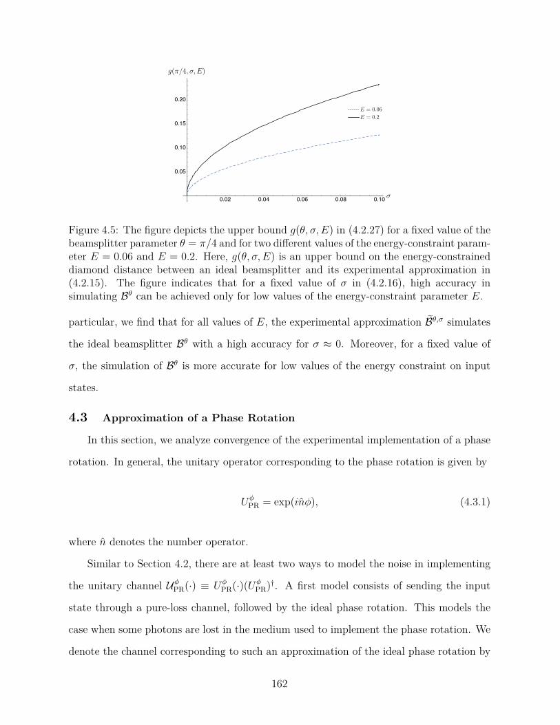
Figure 4.5: The figure depicts the upper bound g ( θ , σ, E ) in (4.2.27) for a fixed value of the

beamsplitter parameter θ = π / 4 and for two different values of the energy-constraint param-

eter E = 0 . 06 and E = 0 . 2 . Here, g ( θ , σ, E ) is an upper bound on the energy-constrained

diamond distance between an ideal beamsplitter and its experimental approximation in

(4.2.15). The figure indicates that for a fixed value of σ in (4.2.16), high accuracy in

simulating B

θ can be achieved only for low values of the energy-constraint parameter E .

particular, we find that for all values of E , the experimental approximation B

θ ,σ simulates

the ideal beamsplitter B

θ with a high accuracy for σ ≈ 0 . Moreover, for a fixed value of

σ , the simulation of B

θ is more accurate for low values of the energy constraint on input

states.

4.3 Approximation of a Phase Rotation

In this section, we analyze convergence of the experimental implementation of a phase

rotation. In general, the unitary operator corresponding to the phase rotation is given by

U

ϕ

PR

= exp( i ˆ nϕ ) ,

(4.3.1)

where ˆ n denotes the number operator.

Similar to Section 4.2, there are at least two ways to model the noise in implementing

the unitary channel U

ϕ

PR( · ) ≡ U

ϕ

PR( · )( U

ϕ

PR)†. A first model consists of sending the input

state through a pure-loss channel, followed by the ideal phase rotation. This models the

case when some photons are lost in the medium used to implement the phase rotation. We

denote the channel corresponding to such an approximation of the ideal phase rotation by

162

U

ϕ,η

PR , such that

U

ϕ,η

PR ( ρ ) ≡ ( U

ϕ

PR

Lη)( ρ ) .

(4.3.2)

Now let ψR A

denote an arbitrary two-mode pure state. Then from unitary invariance of

fidelity, we find that

F ( U

ϕ

PR( ψR A) , U

ϕ,η

PR ( ψR A)) = F ( ψR A

, Lη

A( ψR A)) ,

(4.3.3)

where it is implicit that the identity channel acts on the reference system R . Therefore,

analyzing the convergence of the sequence U

ϕ,η

PR

η ∈ [0 , 1)

to U

ϕ

PR

is equivalent to analyzing the

convergence of a sequence of pure-loss channels to an identity channel. We note that the

same result holds for an ideal displacement unitary and its experimental approximation,

as shown in (4.1.12). Therefore, from the results in Section 4.1, it follows directly that the

sequence U

ϕ,η

PR

η ∈ [0 , 1)

does not converge uniformly to U

ϕ

PR. Rather the convergence holds

in the strong sense. Moreover, the dependence of an estimate of the energy-constrained

diamond distance between U

ϕ,η

PR

and U

ϕ

PR

is given by (4.1.25). From the analysis in Sec-

tion 4.1.3, we conclude that only for low values of the energy constraint E on input states

and high values of η , i.e., low values of the loss, high accuracy in simulating U

ϕ

PR

can be

achieved.

We now consider a phenomenological model to approximate the ideal phase rotation

U

ϕ

PR. In particular, instead of U

ϕ

PR, the following channel is applied:

U

ϕ,σ ≡

∫ 2 π

0

dϕ′ p ( ϕ′ , ϕ, σ, 0 , 2 π ) U

ϕ′

,

(4.3.4)

where p ( ϕ′ , ϕ, σ, 0 , 2 π ) is a truncated normal distribution with location parameter ϕ and

scale parameter σ , as defined in (4.2.16).

Let | α ⟩ be an input coherent state. Then from unitary invariance of fidelity it follows

163

that

F ( U

ϕ( | α ⟩⟨ α | ) , U

ϕ′( | α ⟩⟨ α | )) = F ( | α ⟩⟨ α | , U

ϕ′ − ϕ( | α ⟩⟨ α | )) (4.3.5)

= exp

(

− 2 | α |2(sin( ϕ′ − ϕ ))2

)

, (4.3.6)

which converges to zero as | α |2 → ∞ . Therefore, by an application of the dominated

convergence theorem, it follows that the sequence U

ϕ,σ σ ∈ [0 , ∞ )

does not converge uniformly

to the ideal phase rotation U

ϕ.

The strong convergence of U

ϕ,σ σ ∈ [0 , ∞ )

to U

ϕ follows from arguments similar those

given in (4.2.22) and (4.2.23).

We now provide an estimate of the energy-constrained diamond distance between U

ϕ,σ

and U

ϕ. Consider the following chain of inequalities:

1

2

∥U

ϕ − U

ϕ,σ ∥⋄ E

≤

1

2

∫ 2 π

0

dϕ′ p ( ϕ′ , ϕ, σ, 0 , 2 π ) ∥I − U

ϕ′ − ϕ ∥⋄ E

(4.3.7)

≤

∫ 2 π

0

dϕ′ p ( ϕ′ , ϕ, σ, 0 , 2 π )2

√

E | ϕ′ − ϕ | . (4.3.8)

The first inequality follows from convexity and unitary invariance of the trace distance.

The last inequality follows from [194, Proposition 3.2]. Since the upper bound in (4.3.8) is

exactly same as the upper bound in (4.2.26), we conclude that only for low values of both

the energy constraint E and the scale parameter σ in (4.2.16), high accuracy in simulating

U

ϕ

PR

using U

ϕ,σ can be achieved.

4.4 Approximation of a Single-Mode Squeezer

In this section, we analyze the convergence of the experimental implementation of a

measurement-induced single-mode squeezer from [71] to the ideal single-mode squeezer. We

follow the definition of an ideal single-mode squeezer as in (2.3.56) for ξ = r .

Let ρA

be an input quantum state, and let ˆ xA

and ˆ pA

denote the position- and

momentum-quadrature operators for mode A , respectively. As described in Figure 4.6,

164

the simulation from [71] of S

r( ρA) = S ( r ) ρA

S ( − r ) , such that e− r =

√

η , is given by the

following transformation of the mode operators:

ˆ xA

→

√

η ˆ xA

+

√

1 − η e− rE ˆ x0

E

, (4.4.1)

ˆ pA

→

1

√

η

ˆ pA

, (4.4.2)

where ˆ x0

E

is the position-quadrature operator corresponding to the vacuum state and rE

is the squeezing parameter corresponding to the squeezed vacuum state. We denote the

channel corresponding to the experimental implementation of an ideal single-mode squeezer

by S

η ,rE = S

e− 2 r ,rE . Furthermore, by applying the inverse S

− r of the ideal single-mode

squeezer S

r on the output of S

e− 2 r ,rE , we arrive at the following transformation:

ˆ xout

= ˆ xA

+

√

1 − η

√

η

e− rE ˆ x0

E

, (4.4.3)

ˆ pout

= ˆ pA

. (4.4.4)

We denote the channel induced by the transformation in (4.4.3)–(4.4.4) by Ξη ,rE . Since

all the elements involved in the transformation are Gaussian, the channel Ξη ,rE can be

described by its action on the mean and covariance matrix of the input state ρA. In

particular, there are two 2 × 2 real matrices, the scaling matrix XΞη ,rE

and the noise matrix

YΞη ,rE , which characterize the Gaussian channel Ξη ,rE completely (background on Gaussian

channels can be found in the appendices). It is easy to check that the action of Ξη ,rE does

not change the mean vector of ρA. Therefore, the scaling matrix XΞη ,rE

= I2, where I2

is a

two-dimensional identity matrix. Moreover, the expectation value of the anticommutator

ˆ xA

, ˆ x0

E

is equal to zero, which further implies that the noise matrix YΞη ,rE

has the following

form: YΞη ,rE

= diag ((1 − η ) e− 2 rE /η , 0) .

Let us study the channel Ξη ,rE in further detail. As observed in [195], all single-

mode bosonic Gaussian channels can be categorized into six different canonical forms. In

165

particular, the canonical form ΦB1

has the following XΦB1

and YΦB1

matrices [195]:

XΦB1

= I2

, YΦB1

= diag (0 , 1) .

(4.4.5)

We now show that the channel Ξη ,rE is unitarily equivalent to the canonical form ΦB1

[195].

Let ρ be a quantum state with the covariance matrix Vρ. Then the symplectic matrix

σx

=

0 1

1 0

transforms the covariance matrix Vρ

as follows: V

′

ρ

= σx

Vρ

σx. We then apply

the symplectic transformation corresponding to the symplectic matrix K = diag ( ς , 1 /ς ) ,

where ς =

√

(1 − η ) e− rE /√

η , on the covariance matrix V

′

ρ . The transformed covariance

matrix is given by V

′′

ρ

= K V

′

ρ

K . We now apply the canonical form ΦB1

on the transformed

state, and get the following transformation of the covariance matrix V

′′

ρ

: V

′′′

ρ

= V

′′

ρ

+ YΦB1.

We then apply the symplectic transformation corresponding to the symplectic matrix K

− 1

followed by σx

on V

′′′

ρ

, and get the following final covariance matrix V

final

ρ

:

V

final

ρ

= σx

K

− 1 V

′′

ρ

K

− 1 σx

+ σx

K

− 1 YΦB1

K

− 1 σx

(4.4.6)

= Vρ

+ diag ( ς2 , 0) (4.4.7)

= Vρ

+ diag

(

(1 − η ) e− 2 rE /η , 0

)

, (4.4.8)

which implies that the overall transformation is the same as the action of the channel Ξη ,rE

on the state ρ . Therefore, we have shown that the Gaussian channel Ξη ,rE is unitarily

equivalent by Gaussian input and output unitaries to the canonical form ΦB1 . This gives a

physical interpretation to channels in the class ΦB1 , in terms of the measurement-induced

squeezing approximation from [71].


We now prove that the sequence S

e− 2 r ,rE rE

∈ [0 , ∞ )

does not converge uniformly to

the ideal single-mode squeezer S

r. Let | z ⟩ be a squeezed-vacuum input state with the

covariance matrix V| z ⟩⟨ z |

= diag ( z , 1 /z ) and mean vector µ| z ⟩⟨ z |

= (0 , 0)T, where z ∈ [0 , ∞ ) .

166

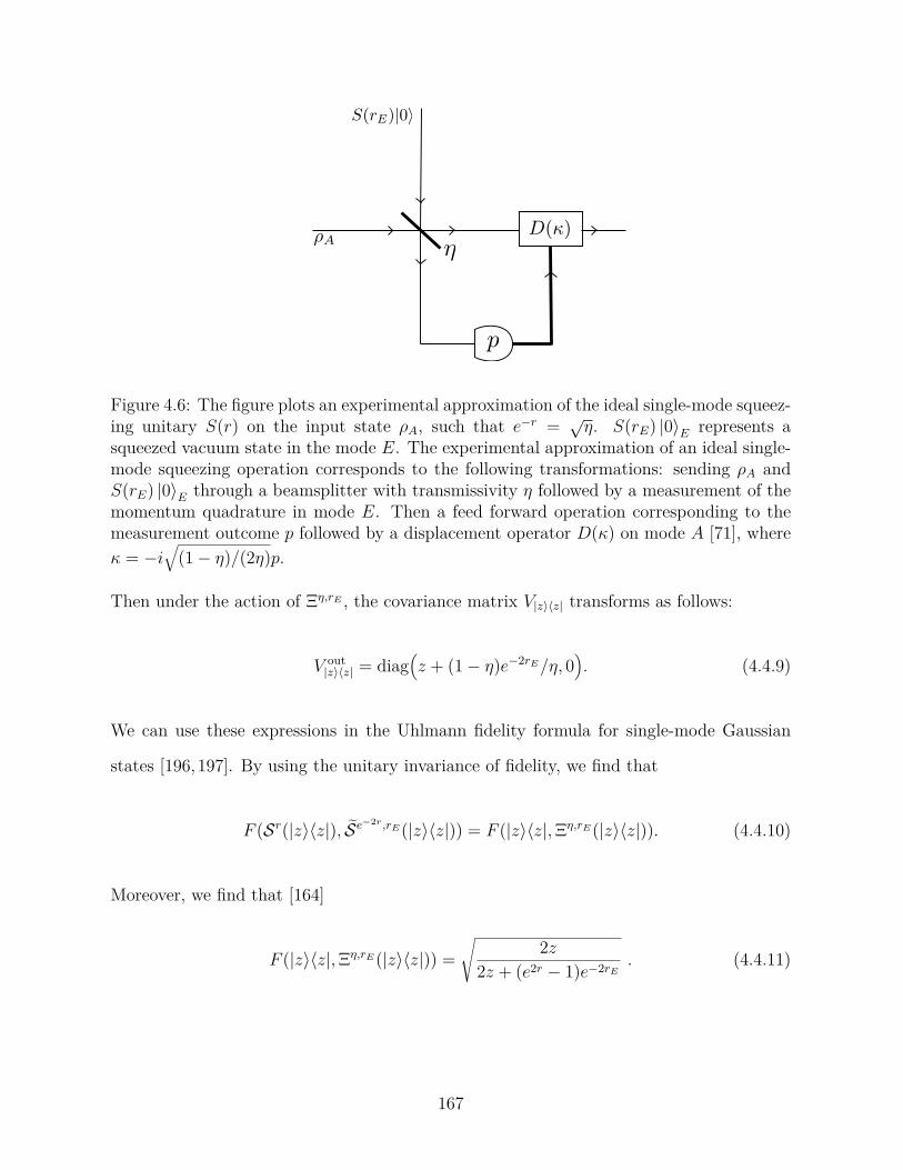
Figure 4.6: The figure plots an experimental approximation of the ideal single-mode squeez-

ing unitary S ( r ) on the input state ρA, such that e− r =

√

η . S ( rE) | 0 ⟩E

represents a

squeezed vacuum state in the mode E . The experimental approximation of an ideal single-

mode squeezing operation corresponds to the following transformations: sending ρA

and

S ( rE) | 0 ⟩E

through a beamsplitter with transmissivity η followed by a measurement of the

momentum quadrature in mode E . Then a feed forward operation corresponding to the

measurement outcome p followed by a displacement operator D ( κ ) on mode A [71], where

κ = − i

√

(1 − η ) / (2 η ) p .

Then under the action of Ξη ,rE , the covariance matrix V| z ⟩⟨ z |

transforms as follows:

V

out

| z ⟩⟨ z |

= diag

(

z + (1 − η ) e− 2 rE /η , 0

)

.

(4.4.9)

We can use these expressions in the Uhlmann fidelity formula for single-mode Gaussian

states [196,197]. By using the unitary invariance of fidelity, we find that

F ( S

r( | z ⟩⟨ z | ) , S

e− 2 r ,rE ( | z ⟩⟨ z | )) = F ( | z ⟩⟨ z | , Ξη ,rE ( | z ⟩⟨ z | )) . (4.4.10)

Moreover, we find that [164]

F ( | z ⟩⟨ z | , Ξη ,rE ( | z ⟩⟨ z | )) =

√

2 z

2 z + ( e2 r − 1) e− 2 rE

.

(4.4.11)

167

Therefore, for fixed rE

limz → 0

F ( S

r( | z ⟩⟨ z | ) , S

e− 2 r ,rE ( | z ⟩⟨ z | )) = 0 ,

(4.4.12)

which implies that the sequence S

e− 2 r ,rE rE

∈ [0 , ∞ )

does not converge uniformly to the ideal

single-mode squeezer transformation S

r.

The reasoning behind (4.4.12) can be intuitively explained as follows: the channel Ξη ,rE

adds noise to the ˆ x quadrature only. Therefore, it can be discriminated from an identity

channel by using an input state that has vanishing noise in the ˆ x quadrature operator.

Since an infinitely squeezed vacuum state (infinitely squeezed in the position quadrature)

satisfies such a condition, then (4.4.12) follows.


We now argue that the sequence S

e− 2 r ,rE rE

∈ [0 , ∞ )

converges to S

r in the strong sense.

Let χρA( x, p ) denote the Wigner characteristic function of the input state ρA. Let ˜ ρout

A

de-

note the state after the action of S

e− 2 r ,rE on ρA: ˜ ρout

A

= S

e− 2 r ,rE ( ρA) . Then the characteristic

function of ˜ ρout

A

is given by

χ˜ ρout

A

( x, p ) = χρA( er x, e− r p ) e− 1

4 ( e2 r − 1) p2 e− 2 rE . (4.4.13)

Moreover, the characteristic function of S

r( ρA) is given by

χS

r( ρA)( x, p ) = χρ( er x, e− r p ) . (4.4.14)

Therefore, for each ρA

∈ D ( HA) , and for all x, p ∈ R

limrE

→∞

χ˜ ρout

A

( x, p ) = χS

r( ρA)( x, p ) . (4.4.15)

168

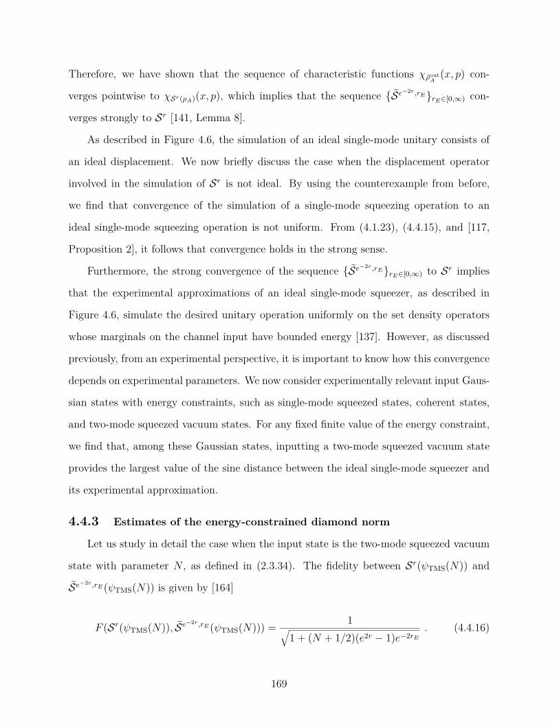
Therefore, we have shown that the sequence of characteristic functions χ˜ ρout

A

( x, p ) con-

verges pointwise to χS

r( ρA)( x, p ) , which implies that the sequence S

e− 2 r ,rE rE

∈ [0 , ∞ )

con-

verges strongly to S

r [141, Lemma 8].

As described in Figure 4.6, the simulation of an ideal single-mode unitary consists of

an ideal displacement. We now briefly discuss the case when the displacement operator

involved in the simulation of S

r is not ideal. By using the counterexample from before,

we find that convergence of the simulation of a single-mode squeezing operation to an

ideal single-mode squeezing operation is not uniform. From (4.1.23), (4.4.15), and [117,

Proposition 2], it follows that convergence holds in the strong sense.

Furthermore, the strong convergence of the sequence S

e− 2 r ,rE rE

∈ [0 , ∞ )

to S

r implies

that the experimental approximations of an ideal single-mode squeezer, as described in

Figure 4.6, simulate the desired unitary operation uniformly on the set density operators

whose marginals on the channel input have bounded energy [137]. However, as discussed

previously, from an experimental perspective, it is important to know how this convergence

depends on experimental parameters. We now consider experimentally relevant input Gaus-

sian states with energy constraints, such as single-mode squeezed states, coherent states,

and two-mode squeezed vacuum states. For any fixed finite value of the energy constraint,

we find that, among these Gaussian states, inputting a two-mode squeezed vacuum state

provides the largest value of the sine distance between the ideal single-mode squeezer and

its experimental approximation.

4.4.3 Estimates of the energy-constrained diamond norm

Let us study in detail the case when the input state is the two-mode squeezed vacuum

state with parameter N , as defined in (2.3.34). The fidelity between S

r( ψTMS( N )) and

S

e− 2 r ,rE ( ψTMS( N )) is given by [164]

F ( S

r( ψTMS( N )) , S

e− 2 r ,rE ( ψTMS( N ))) =

1

√

1 + ( N + 1 / 2)( e2 r − 1) e− 2 rE

. (4.4.16)

169

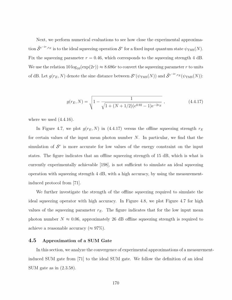
Next, we perform numerical evaluations to see how close the experimental approxima-

tion S

e− 2 r ,rE is to the ideal squeezing operation S

r for a fixed input quantum state ψTMS( N ) .

Fix the squeezing parameter r = 0 . 46 , which corresponds to the squeezing strength 4 dB.

We use the relation 10 log10(exp(2 r )) ≈ 8 . 686 r to convert the squeezing parameter r to units

of dB. Let g ( rE

, N ) denote the sine distance between S

r( ψTMS( N )) and S

e− 2 r ,rE ( ψTMS( N )) :

g ( rE

, N ) =

√√√√

1 −

1

√

1 + ( N + 1 / 2)( e0 . 92 − 1) e− 2 rE

, (4.4.17)

where we used (4.4.16).

In Figure 4.7, we plot g ( rE

, N ) in (4.4.17) versus the offline squeezing strength rE

for certain values of the input mean photon number N . In particular, we find that the

simulation of S

r is more accurate for low values of the energy constraint on the input

states. The figure indicates that an offline squeezing strength of 15 dB, which is what is

currently experimentally achievable [198], is not sufficient to simulate an ideal squeezing

operation with squeezing strength 4 dB, with a high accuracy, by using the measurement-

induced protocol from [71].

We further investigate the strength of the offline squeezing required to simulate the

ideal squeezing operator with high accuracy. In Figure 4.8, we plot Figure 4.7 for high

values of the squeezing parameter rE. The figure indicates that for the low input mean

photon number N ≈ 0 . 06 , approximately 26 dB offline squeezing strength is required to

achieve a reasonable accuracy ( ≈ 97% ).

4.5 Approximation of a SUM Gate

In this section, we analyze the convergence of experimental approximations of a measurement-

induced SUM gate from [71] to the ideal SUM gate. We follow the definition of an ideal

SUM gate as in (2.3.58).

170

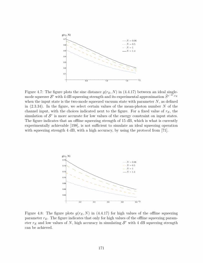
rE

g(rE, N)

Figure 4.7: The figure plots the sine distance g ( rE

, N ) in (4.4.17) between an ideal single-

mode squeezer S

r with 4 dB squeezing strength and its experimental approximation S

e− 2 r ,rE

when the input state is the two-mode squeezed vacuum state with parameter N , as defined

in (2.3.34). In the figure, we select certain values of the mean-photon number N of the

channel input, with the choices indicated next to the figure. For a fixed value of rE, the

simulation of S

r is more accurate for low values of the energy constraint on input states.

The figure indicates that an offline squeezing strength of 15 dB, which is what is currently

experimentally achievable [198], is not sufficient to simulate an ideal squeezing operation

with squeezing strength 4 dB, with a high accuracy, by using the protocol from [71].

rE

g(rE, N)

Figure 4.8: The figure plots g ( rE

, N ) in (4.4.17) for high values of the offline squeezing

parameter rE. The figure indicates that only for high values of the offline squeezing param-

eter rE

and low values of N , high accuracy in simulating S

r with 4 dB squeezing strength

can be achieved.

171

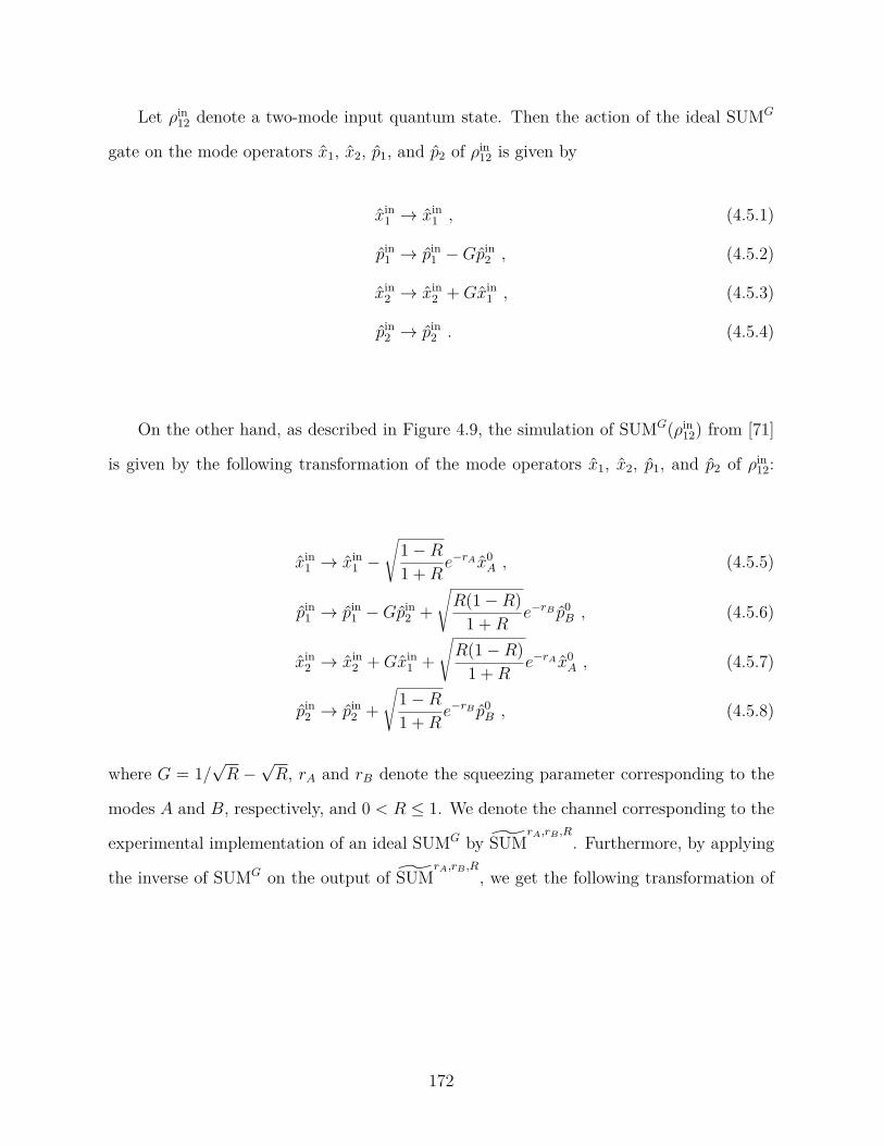
Let ρin

12

denote a two-mode input quantum state. Then the action of the ideal SUMG

gate on the mode operators ˆ x1, ˆ x2, ˆ p1, and ˆ p2

of ρin

12

is given by

ˆ xin

1

→ ˆ xin

1

, (4.5.1)

ˆ pin

1

→ ˆ pin

1

− G ˆ pin

2

, (4.5.2)

ˆ xin

2

→ ˆ xin

2

+ G ˆ xin

1

, (4.5.3)

ˆ pin

2

→ ˆ pin

2

. (4.5.4)

On the other hand, as described in Figure 4.9, the simulation of SUMG( ρin

12) from [71]

is given by the following transformation of the mode operators ˆ x1, ˆ x2, ˆ p1, and ˆ p2

of ρin

12:

ˆ xin

1

→ ˆ xin

1

−

√

1 − R

1 + R

e− rA ˆ x0

A

, (4.5.5)

ˆ pin

1

→ ˆ pin

1

− G ˆ pin

2

+

√

R (1 − R )

1 + R

e− rB ˆ p0

B

, (4.5.6)

ˆ xin

2

→ ˆ xin

2

+ G ˆ xin

1

+

√

R (1 − R )

1 + R

e− rA ˆ x0

A

, (4.5.7)

ˆ pin

2

→ ˆ pin

2

+

√

1 − R

1 + R

e− rB ˆ p0

B

, (4.5.8)

where G = 1 /√

R −

√

R , rA

and rB

denote the squeezing parameter corresponding to the

modes A and B , respectively, and 0 < R ≤ 1 . We denote the channel corresponding to the

experimental implementation of an ideal SUMG by SUM

rA

,rB

,R. Furthermore, by applying

the inverse of SUMG on the output of SUM

rA

,rB

,R, we get the following transformation of

172

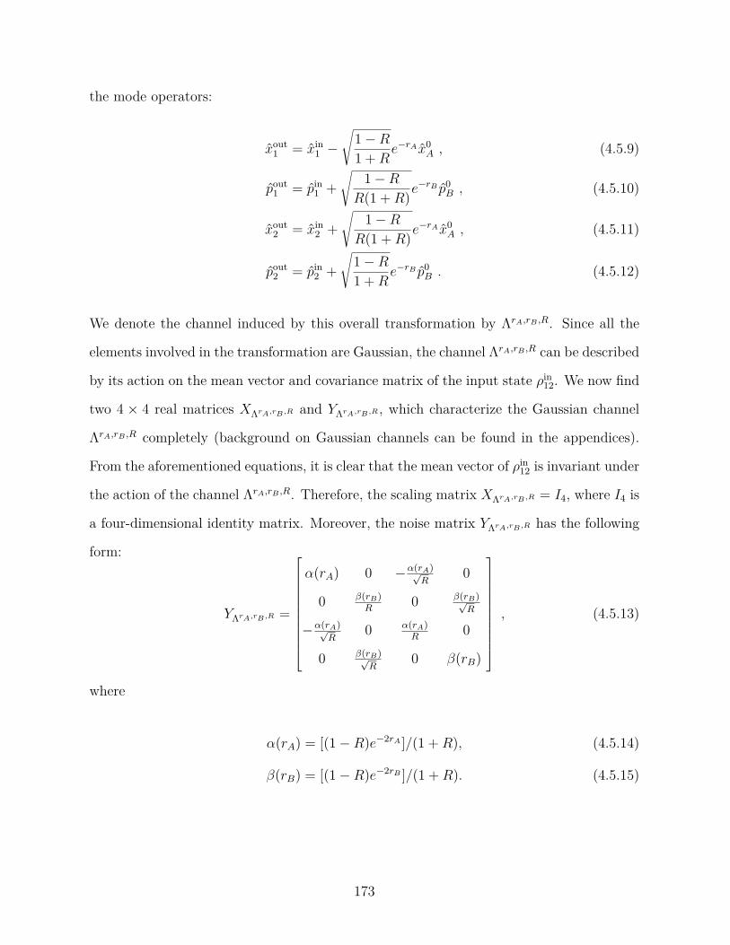
the mode operators:

ˆ xout

1

= ˆ xin

1

−

√

1 − R

1 + R

e− rA ˆ x0

A

, (4.5.9)

ˆ pout

1

= ˆ pin

1

+

√

1 − R

R (1 + R )

e− rB ˆ p0

B

, (4.5.10)

ˆ xout

2

= ˆ xin

2

+

√

1 − R

R (1 + R )

e− rA ˆ x0

A

, (4.5.11)

ˆ pout

2

= ˆ pin

2

+

√

1 − R

1 + R

e− rB ˆ p0

B

. (4.5.12)

We denote the channel induced by this overall transformation by ΛrA

,rB

,R. Since all the

elements involved in the transformation are Gaussian, the channel ΛrA

,rB

,R can be described

by its action on the mean vector and covariance matrix of the input state ρin

12. We now find

two 4 × 4 real matrices XΛrA

,rB

,R and YΛrA

,rB

,R , which characterize the Gaussian channel

ΛrA

,rB

,R completely (background on Gaussian channels can be found in the appendices).

From the aforementioned equations, it is clear that the mean vector of ρin

12

is invariant under

the action of the channel ΛrA

,rB

,R. Therefore, the scaling matrix XΛrA

,rB

,R = I4, where I4

is

a four-dimensional identity matrix. Moreover, the noise matrix YΛrA

,rB

,R has the following

form:

YΛrA

,rB

,R =

α ( rA) 0 −

α ( rA)

√

R

0

0

β ( rB)

R

0

β ( rB)

√

R

−

α ( rA)

√

R

0

α ( rA)

R

0

0

β ( rB)

√

R

0 β ( rB)

,

(4.5.13)

where

α ( rA) = [(1 − R ) e− 2 rA ] / (1 + R ) , (4.5.14)

β ( rB) = [(1 − R ) e− 2 rB ] / (1 + R ) . (4.5.15)

173

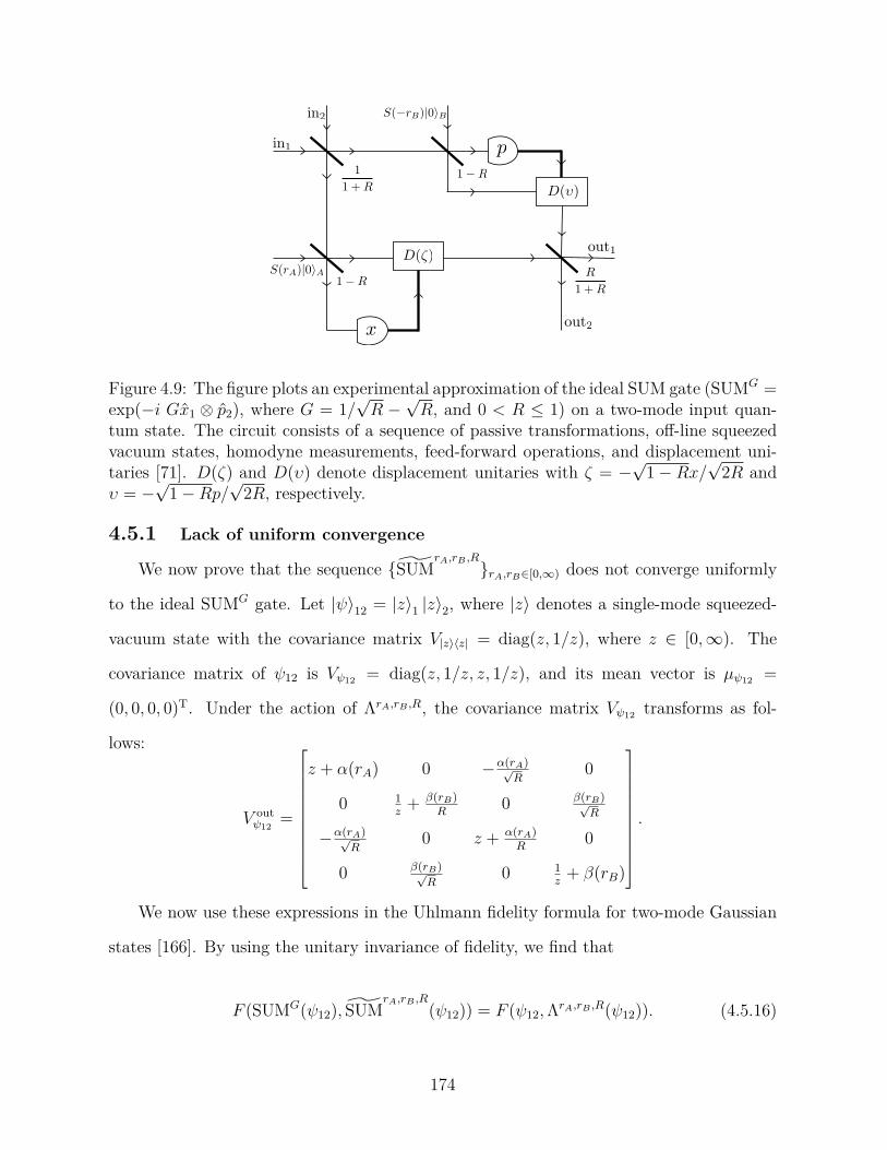
Figure 4.9: The figure plots an experimental approximation of the ideal SUM gate (SUMG =

exp( − i G ˆ x1

⊗ ˆ p2) , where G = 1 /√

R −

√

R , and 0 < R ≤ 1 ) on a two-mode input quan-

tum state. The circuit consists of a sequence of passive transformations, off-line squeezed

vacuum states, homodyne measurements, feed-forward operations, and displacement uni-

taries [71]. D ( ζ ) and D ( υ ) denote displacement unitaries with ζ = −√

1 − R x/√

2 R and

υ = −√

1 − R p/√

2 R , respectively.


We now prove that the sequence SUM

rA

,rB

,R

rA

,rB

∈ [0 , ∞ )

does not converge uniformly

to the ideal SUMG gate. Let | ψ ⟩12

= | z ⟩1

| z ⟩2, where | z ⟩ denotes a single-mode squeezed-

vacuum state with the covariance matrix V| z ⟩⟨ z |

= diag ( z , 1 /z ) , where z ∈ [0 , ∞ ) . The

covariance matrix of ψ12

is Vψ12

= diag ( z , 1 /z , z , 1 /z ) , and its mean vector is µψ12

=

(0 , 0 , 0 , 0)T. Under the action of ΛrA

,rB

,R, the covariance matrix Vψ12

transforms as fol-

lows:

V

out

ψ12

=

z + α ( rA) 0 −

α ( rA)

√

R

0

0

1

z

+

β ( rB)

R

0

β ( rB)

√

R

−

α ( rA)

√

R

0 z +

α ( rA)

R

0

0

β ( rB)

√

R

0

1

z

+ β ( rB)

.

We now use these expressions in the Uhlmann fidelity formula for two-mode Gaussian

states [166]. By using the unitary invariance of fidelity, we find that

F ( SUMG( ψ12) , SUM

rA

,rB

,R( ψ12)) = F ( ψ12

, ΛrA

,rB

,R( ψ12)) . (4.5.16)

174

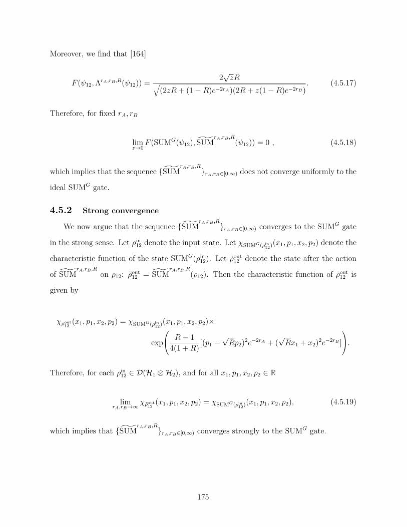
Moreover, we find that [164]

F ( ψ12

, ΛrA

,rB

,R( ψ12)) =

2√

z R

√

(2 z R + (1 − R ) e− 2 rA)(2 R + z (1 − R ) e− 2 rB )

. (4.5.17)

Therefore, for fixed rA

, rB

limz → 0

F ( SUMG( ψ12) , SUM

rA

,rB

,R( ψ12)) = 0 , (4.5.18)

which implies that the sequence SUM

rA

,rB

,R

rA

,rB

∈ [0 , ∞ )

does not converge uniformly to the

ideal SUMG gate.


We now argue that the sequence SUM

rA

,rB

,R

rA

,rB

∈ [0 , ∞ )

converges to the SUMG gate

in the strong sense. Let ρin

12

denote the input state. Let χSUMG( ρin

12)( x1

, p1

, x2

, p2) denote the

characteristic function of the state SUMG( ρin

12) . Let ˜ ρout

12

denote the state after the action

of SUM

rA

,rB

,R

on ρ12: ˜ ρout

12

= SUM

rA

,rB

,R( ρ12) . Then the characteristic function of ˜ ρout

12

is

given by

χ˜ ρout

12

( x1

, p1

, x2

, p2) = χSUMG( ρin

12)( x1

, p1

, x2

, p2) ×

exp

R − 1

4(1 + R ) [( p1

−

√

R p2)2 e− 2 rA + (

√

R x1

+ x2)2 e− 2 rB ]

.

Therefore, for each ρin

12

∈ D ( H1

⊗ H2) , and for all x1

, p1

, x2

, p2

∈ R

limrA

,rB

→∞

χ˜ ρout

12

( x1

, p1

, x2

, p2) = χSUMG( ρin

12)( x1

, p1

, x2

, p2) , (4.5.19)

which implies that SUM

rA

,rB

,R

rA

,rB

∈ [0 , ∞ )

converges strongly to the SUMG gate.

175

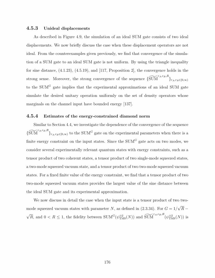
4.5.3 Unideal displacements

As described in Figure 4.9, the simulation of an ideal SUM gate consists of two ideal

displacements. We now briefly discuss the case when these displacement operators are not

ideal. From the counterexamples given previously, we find that convergence of the simula-

tion of a SUM gate to an ideal SUM gate is not uniform. By using the triangle inequality

for sine distance, (4.1.23), (4.5.19), and [117, Proposition 2], the convergence holds in the

strong sense. Moreover, the strong convergence of the sequence SUM

rA

,rB

,R

rA

,rB

∈ [0 , ∞ )

to the SUMG gate implies that the experimental approximations of an ideal SUM gate

simulate the desired unitary operation uniformly on the set of density operators whose

marginals on the channel input have bounded energy [137].

4.5.4 Estimates of the energy-constrained diamond norm

Similar to Section 4.4, we investigate the dependence of the convergence of the sequence

SUM

rA

,rB

,R

rA

,rB

∈ [0 , ∞ )

to the SUMG gate on the experimental parameters when there is a

finite energy constraint on the input states. Since the SUMG gate acts on two modes, we

consider several experimentally relevant quantum states with energy constraints, such as a

tensor product of two coherent states, a tensor product of two single-mode squeezed states,

a two-mode squeezed vacuum state, and a tensor product of two two-mode squeezed vacuum

states. For a fixed finite value of the energy constraint, we find that a tensor product of two

two-mode squeezed vacuum states provides the largest value of the sine distance between

the ideal SUM gate and its experimental approximation.

We now discuss in detail the case when the input state is a tensor product of two two-

mode squeezed vacuum states with parameter N , as defined in (2.3.34). For G = 1 /√

R −

√

R , and 0 < R ≤ 1 , the fidelity between SUMG( ψ

⊗ 2

TMS( N )) and SUM

rA

,rB

,R( ψ

⊗ 2

TMS( N )) is

176

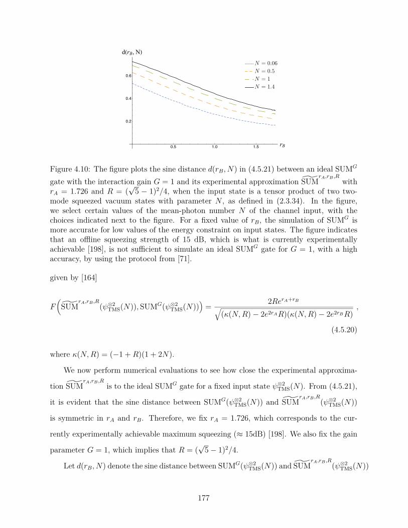
rB

d(rB, N)

Figure 4.10: The figure plots the sine distance d ( rB

, N ) in (4.5.21) between an ideal SUMG

gate with the interaction gain G = 1 and its experimental approximation SUM

rA

,rB

,R

with

rA

= 1 . 726 and R = (√

5 − 1)2 / 4 , when the input state is a tensor product of two two-

mode squeezed vacuum states with parameter N , as defined in (2.3.34). In the figure,

we select certain values of the mean-photon number N of the channel input, with the

choices indicated next to the figure. For a fixed value of rB, the simulation of SUMG is

more accurate for low values of the energy constraint on input states. The figure indicates

that an offline squeezing strength of 15 dB, which is what is currently experimentally

achievable [198], is not sufficient to simulate an ideal SUMG gate for G = 1 , with a high

accuracy, by using the protocol from [71].

given by [164]

F

(

SUM

rA

,rB

,R( ψ

⊗ 2

TMS( N )) , SUMG( ψ

⊗ 2

TMS( N ))

)

=

2 R erA+ rB

√

( κ ( N , R ) − 2 e2 rA R )( κ ( N , R ) − 2 e2 rB R )

,

(4.5.20)

where κ ( N , R ) = ( − 1 + R )(1 + 2 N ) .

We now perform numerical evaluations to see how close the experimental approxima-

tion SUM

rA

,rB

,R

is to the ideal SUMG gate for a fixed input state ψ

⊗ 2

TMS( N ) . From (4.5.21),

it is evident that the sine distance between SUMG( ψ

⊗ 2

TMS( N )) and SUM

rA

,rB

,R( ψ

⊗ 2

TMS( N ))

is symmetric in rA

and rB. Therefore, we fix rA

= 1 . 726 , which corresponds to the cur-

rently experimentally achievable maximum squeezing ( ≈ 15 dB) [198]. We also fix the gain

parameter G = 1 , which implies that R = (√

5 − 1)2 / 4 .

Let d ( rB

, N ) denote the sine distance between SUMG( ψ

⊗ 2

TMS( N )) and SUM

rA

,rB

,R( ψ

⊗ 2

TMS( N ))

177

for R = (√

5 − 1)2 / 4 and rA

= 1 . 726 :

d ( rB

, N ) =

√√√√

1 −

2 R erA+ rB

√

( κ ( N , R ) − 2 e2 rA R )( κ ( N , R ) − 2 e2 rB R )

, (4.5.21)

where we used (4.5.20).

In Figure 4.10, we plot d ( rB

, N ) in (4.5.21) versus the offline squeezing strength rB

for

certain values of the input mean photon number N . Similar to the results in Sections 4.1

and 4.4, we find that the simulation of SUMG is more accurate for low values of the energy

constraint on input states. Moreover, even with a low mean photon number N = 0 . 06 of

the input states and with the currently experimentally achievable offline squeezing strength

of 15 dB, only approximately 83% accuracy in simulating the ideal SUMG gate for G = 1

can be achieved.

It is an open question to establish analytical bounds to quantify the performance of

these experimental approximations of a SUM gate with respect to an energy-constrained

distance measure.

4.6 Approximation of One- and Two-Mode Gaussian Unitaries

In this section, we show that a sequence of one-mode Gaussian channels does not

converge uniformly to a one-mode Gaussian unitary. The same is true for the two-mode

case. However, convergence occurs in the strong sense.

We begin by defining a set of matrices that characterizes all n -mode Gaussian channels.

Let G

X ,Y denote an n -mode Gaussian channel, which is completely characterized by two

2 n × 2 n real matrices X and Y . For G

X ,Y to be a physical channel, the X and Y matrices

must be such that

Y + i Ω ≥ iX Ω X

T , Y = Y

T . (4.6.1)

178

Let Sn

denote a set of a pair of matrices X and Y that satisfy (4.6.1), i.e.,

Sn

= ( X , Y ) : Y + i Ω ≥ iX Ω X

T , Y = Y

T , (4.6.2)

where n in the subscript of Sn

indicates that the set Sn

consists of a pair of 2 n × 2 n real

matrices.

Let UA → B

denote a single-mode Gaussian unitary transformation. Suppose that an

experimental approximation of UA → B

is a single-mode Gaussian channel U

X ,Y

A → B, which is

completely characterized by two 2 × 2 real matrices X and Y . We now show that the

sequence U

X ,Y ( X ,Y ) ∈ S1

does not converge uniformly to U , where S1

is given by (4.6.2) for

n = 1 . Let ψR A(¯ n ) denote a two-mode squeezed vacuum state with parameter ¯ n , as defined

in (2.3.34). Let G

X ,Y

A → B

= U

− 1 U

X ,Y

A → B

denote the overall Gaussian channel. Let

X =

x11

x12

x21

x22

, Y =

y11

y12

y12

y22

. (4.6.3)

Then from the unitary invariance of fidelity, we find that

F ( UA → B( ψR A(¯ n )) , U

X ,Y

A → B( ψR A(¯ n ))) = F ( ψR A(¯ n ) , G

X ,Y

A → B( ψR A(¯ n ))) , (4.6.4)

where it is implicit that an identity channel acts on the reference system R .

By expanding F ( UA → B( ψR A(¯ n )) , U

X ,Y

A → B( ψR A(¯ n ))) about ¯ n = ∞ , we find that [164]

F ( UA → B( ψR A(¯ n )) , U

X ,Y

A → B( ψR A(¯ n ))) =

1

( − 1 + x11

+ x12

x21

+ x22

− x11

x22)¯ n2

+ O (1 / ¯ n )3 .

(4.6.5)

Therefore,

lim¯ n →∞

F ( UA → B( ψR A(¯ n )) , U

X ,Y

A → B( ψR A(¯ n ))) = 0 .

(4.6.6)

179

Using (2.4.12) and (4.6.6), we find that

lim¯ n →∞

∥UA → B

− U

X ,Y

A → B

∥⋄

= 2 ,

(4.6.7)

which implies that the sequence U

X ,Y ( X ,Y ) ∈ S1

does not converge uniformly to the ideal

single-mode Gaussian unitary transformation UA → B.

Similarly, it can be shown that a sequence of two-mode Gaussian channels does not

converge uniformly to an ideal two-mode Gaussian unitary transformation [164].

On the other hand, as a consequence of [117, Proposition 1], the convergence holds in

the strong sense for both the one- and two-mode case, and in fact for the general n -mode

case.

4.7 Conclusion

In this chapter, using different performance metrics we analyzed how well an ideal dis-

placement operator, an ideal single-mode squeezer, and an ideal SUM gate can be simulated

experimentally. In particular, we proved that none of these experimental approximations

converge uniformly to the ideal Gaussian processes. Rather, convergence occurs in the

strong sense.

We also discussed the notion of uniform convergence on the set of density operators

whose marginals on the channel input have bounded energy, which is the most relevant

from an experimental perspective, given that experiments are generally energy sensitive.

In particular, we reduced the problem of distinguishing an ideal displacement operator

from its experimental approximation to the problem of distinguishing a pure-loss channel

from an ideal channel. We provided an analytic expression for the energy-constrained sine

distance between an ideal displacement unitary and its approximation in terms of exper-

imental parameters, by using the result of [186]. Moreover, we established two different

lower bounds on the energy-constrained diamond distance between an ideal displacement

operator and its experimental approximation for low values of the energy constraint on

180

input states. These bounds could be used to determine the requirements needed to im-

plement a displacement operator to any desired accuracy. The displacement operator is

ubiquitous in quantum optics and plays a critical role in CV quantum teleportation, CV

quantum error correction and quantum computation, and quantum metrology. Therefore,

quantification of the accuracy in simulating a displacement operator is important for several

practical applications.

We then introduced two different methods to model the noise or loss in implement-

ing both beamsplitters and phase rotations. For these models, we established analytical

bounds on the energy-constrained diamond distance between these ideal gates and their ex-

perimental approximations. These bounds are relevant for characterizing the performance

of any experiment consisting of beamsplitters and phase rotations.

Similarly, we discussed the notion of uniform convergence on the set of density operators

whose marginals on the channel input have bounded energy for experimental approxima-

tions of both the single-mode squeezing unitary and the SUM gate. We considered several

experimentally relevant input quantum states and studied how close these experimental

approximations are to the ideal quantum processes. It is an interesting open question to

determine the optimal value of energy-constrained distance measures and the correspond-

ing optimal state to completely characterize these experimental approximations of the ideal

quantum processes.

In this chapter, homodyne measurements involved in simulating a single-mode squeezer

and a SUM gate were considered ideal. We expect that the well-known experimental ap-

proximation of homodyne detection converges strongly to ideal homodyne detection, based

on the calculation of [199, Appendix K], and we also expect that the experimental ap-

proximation will not converge uniformly. However, it is an open question to determine the

optimal value of energy-constrained distance measures and corresponding optimal states

when homodyne measurements involved in these simulations are not ideal. Another in-

teresting direction is to use these results to study the error propagation in an experiment

181

based on quantum optical elements.

182

CHAPTER 5

OPTIMAL TESTS FOR CONTINUOUS-VARIABLE

QUANTUM TELEPORTATION AND PHOTODETECTORS

This chapter presents applications of energy-constrained distance measures to deter-

mine optimal tests for benchmarking continuous-variable (CV) teleportation and photode-

tectors. Our first main contribution is the reduction of the problem of estimating the

energy-constrained channel fidelity between ideal teleportation and its experimental imple-

mentation to a quadratic program over an infinite number of variables. We then define a

truncated version of this quadratic program and prove that it is a convex optimization prob-

lem. We numerically solve it using a MATLAB package, which employs the interior-point

method [200]. We also provide analytical solutions by invoking the Karush-Kuhn-Tucker

(KKT) conditions [86,87]. We then argue that these solutions to the truncated versions of

quadratic programs also optimize the energy-constrained channel fidelity defined over an

infinite-dimensional, separable Hilbert space, i.e., without any truncation.

One of our main findings is that among all pure bipartite states, an entangled super-

position of twin-Fock states saturating the energy constraint is optimal for distinguishing

ideal CV teleportation from its experimental implementation. Our results thus provide an

experimental strategy to verify whether an unconditional experimental teleportation with

high accuracy is possible [76]. Here, by unconditional teleportation, we imply that telepor-

tation of any unknown, energy-constrained state should be feasible. We also discuss why

previous proposals based on the teleportation of coherent states or other commonly used

states are not suitable for quantifying the performance of unconditional teleportation.

We then provide a solution to the energy-constrained diamond distance between a

photodetector and its experimental approximation. We model the noisy version of a pho-

todetector as a pure-loss channel followed by an ideal photodetector. We will prove that

number-diagonal states optimize the energy-constrained diamond distance and show that

183

entanglement is not required for the optimal distinguishability of the ideal photodetector

from its experimental implementation.

The rest of the chapter is organized as follows. We present our results on an optimal

test for CV teleportation in Section 5.1. We next present results on an optimal test for

photodetectors in Section 5.2. Finally, we conclude and summarize open problems in

Section 5.3.

5.1 Continuous-Variable Quantum Teleportation

In this section, we characterize the performance of continuous-variable (CV) quantum

teleportation in terms of the energy-constrained channel fidelity between ideal CV telepor-

tation and its experimental approximation, the latter being the protocol from [37].

Let A denote the input mode. Ideal CV teleportation induces an identity channel

on input states, which we denote by IA → B. On the other hand, an experimental imple-

mentation of CV teleportation realizes an additive-noise channel T

ξ

A → B

with the variance

parameter ξ , as defined in (2.3.85), which quantifies unideal squeezing and unideal detection

in the teleportation protocol [37].

The energy-constrained channel fidelity between the identity channel and an additive-

noise channel with parameter ξ is given by:

FE( IA → B

, T

ξ

A → B) ≡ inf

ρR A:Tr(ˆ nA

ρA) ≤ E

F ( ρR A

, T

ξ

A( ρR A)) ,

(5.1.1)

where ρR A

= D ( HR A) , ρA

= Tr( ρR A) , and ˆ n =

∑∞

n =0

n | n ⟩⟨ n | .

From joint concavity of root fidelity and monotonicity of the square function, the

optimization in (5.1.1) can be reduced to pure states satisfying the energy constraint as

follows:

FE( IA

, T

ξ

A) ≡ inf

ϕR A:Tr(ˆ nA

ϕA) ≤ E

F ( ϕR A

, T

ξ

A( ϕR A)) ,

(5.1.2)

where ϕR A

is a pure state and R is a single-mode reference system.

We now argue that the optimization in (5.1.2) can be further restricted to pure states

184

that are entangled superpositions of twin-Fock states, satisfying the energy constraint. Let

ϕA

= Tr R( ϕR A) . Consider the following phase averaging of ϕA:

ψA

≡

1

2 π

∫ 2 π

0

dθ ei ˆ nθ ϕA

e− i ˆ nθ (5.1.3)

=

∞∑

n =0

| n ⟩⟨ n | ϕA

| n ⟩⟨ n | (5.1.4)

=

∞∑

n =0

λ2

n

| n ⟩⟨ n |A

, (5.1.5)

where λ2

n

≡ ⟨ n | ϕA

| n ⟩ .

Then from isometric invariance and monotonicity of fidelity, and from the joint phase

covariance of IA

and T

ξ

A , it follows that (see e.g., [93, 153])

F ( ψR A

, ( IR

⊗ T

ξ

A)( ψR A)) ≤ F ( ϕR A

, ( IR

⊗ T

ξ

A)( ϕR A)) ,

(5.1.6)

where ψR A

= | ψ ⟩⟨ ψ |R A

is a purification of ψA

in (5.1.5).

Since the phase averaging operation does not change the mean photon number, we

get that Tr(ˆ nψA) = Tr(ˆ nϕA) [93]. Thus, combining (5.1.2) and (5.1.6) further reduces the

optimization in (5.1.2) as follows:

FE( IA

, T

ξ

A) = inf

ψR A:Tr(ˆ nA

ψA) ≤ E

F ( ψR A

, T

ξ

A( ψR A)) ,

(5.1.7)

where

| ψ ⟩R A

=

∞∑

n =0

λn

| n ⟩R

| n ⟩A

,

(5.1.8)

for some λn

∈ R+ such that

∑∞

n =0

λ2

n

= 1 and

∑∞

n =0

λ2

n

n ≤ E . As discussed in Chapter 2,

we call | ψ ⟩R A

in (5.1.8) an entangled superposition of twin-Fock states.

We now show that the optimization in (5.1.7) can be formulated as a quadratic program

(see [201] for a review on quadratic programs). Note that the adjoint of a quantum-limited

185

amplifier channel A1 /η is related to a pure-loss channel Lη in the following sense [202]:

( A1 /η)† = η Lη .

(5.1.9)

Then we get

F ( ψR A

, T

ξ

A( ψR A)) = Tr

(

ψR A

T

ξ

A( ψR A)

)

(5.1.10)

= Tr

(

ψR A( A1 /η Lη)( ψR A)

)

(5.1.11)

= η Tr

(

( Lη( ψR A))2

)

(5.1.12)

= η Tr

(

( L1 − η( ψA))2

)

, (5.1.13)

where

ψA

=

∞∑

n =0

λ2

n

| n ⟩⟨ n |A

.

(5.1.14)

The third equality follows from (5.1.9) and the last equality holds because the marginals

of a pure bipartite state have the same purity, where the purity of a state ρ is defined as

Tr( ρ2) .

To simplify (5.1.13) further, we recall that the action of a pure-loss channel L1 − η on

ψA

above is as follows:

L1 − η

A

( ψA) =

∞∑

n =0

λ2

n

n∑

k =0

(n

k

)

(1 − η )k η

n − k | k ⟩⟨ k |A

. (5.1.15)

Let pn

≡ λ2

n

and p ≡ ( p0

, p1

, . . . ) . Then by using (5.1.15) in (5.1.13), we find that

F ( ψR A

, T

ξ

A( ψR A)) =

∞∑

n,m =0

pn

pm

min n,m ∑

k =0

(n

k

)(m

k

)

ξ2 k

(1 + ξ )n + m +1

(5.1.16)

≡ f ( p ) (5.1.17)

186

where we used

η = 1 / (1 + ξ ) .

(5.1.18)

Henceforth, we denote F ( ψR A

, T

ξ

A → B( ψR A)) as f ( p ) , as indicated in (5.1.17).

Therefore, the problem of estimating the energy-constrained channel fidelity between

ideal CV teleportation and its experimental implementation reduces to the following quadratic

optimization problem:

FE( IA

, T

ξ

A) =

inf p

f ( p )

subject to

∑∞

n =0

npn

≤ E ,

pn

≥ 0 , ∀ n ∈ Z≥ 0 ,

∑∞

n =0

pn

= 1 .

(5.1.19)

Solutions to quadratic programs can be obtained numerically by using a MATLAB

package that employs the interior-point method [200]. Moreover, analytical solutions can be

calculated by invoking the Karush-Kuhn-Tucker (KKT) conditions [86,87]. However, these

methods are suitable for solving optimization problems over a finite number of variables.

Therefore, we first define a truncated version of the energy-constrained channel fidelity

between two quantum channels, which is equivalent to a quadratic program over a finite

number of variables for the task of distinguishing the identity channel from an additive-noise

channel. We argue below that for finite E and high values of the truncation parameter, it

is sufficient to find solutions on a truncated Hilbert space.

Energy-constrained channel fidelity over a truncated Hilbert space . Let M de-

note the truncation parameter, and let HM

denote an ( M + 1) -dimensional Fock space

| 0 ⟩ , | 1 ⟩ , . . . , | M ⟩ . Let ωA

∈ D ( HM) . We define the energy-constrained channel fidelity

187

between two quantum channels NA → B

and MA → B

on a truncated Hilbert space as

FE ,M( NA → B

, MA → B) ≡ inf

ωR A

∈D ( HR

⊗HM ):

Tr(ˆ nωA) ≤ E

F ( N ( ωR A) , M ( ωR A)) ,

(5.1.20)

where ωR A

is an extension of ωA. Moreover, it is implicit that the identity channel acts

on the reference system R . Similar to the previous case, it suffices to optimize over pure

bipartite states of systems R and A , with system R isomorphic to system A , so that the

dimension of R can be set to M + 1 .

Since the optimization in (5.1.20) is over a truncated space instead of an infinite-

dimensional separable Hilbert space, we get

FE( NA → B

, MA → B) ≤ FE ,M( NA → B

, MA → B) .

(5.1.21)

We now establish a lower bound on FE( NA → B

, MA → B) in terms of FE ,M( NA → B

, MA → B) ,

which combining with (5.1.21) will imply that solutions to (5.1.19) can be obtained by solv-

ing a quadratic program on a truncated Hilbert space. For completeness we first argue that

the set of density operators acting on a truncated Hilbert space with a finite mean energy

constraint is dense in the set of density operators acting on an infinite-dimensional Hilbert

space and with the same mean energy constraint [92]. Let ρR A

denote a density operator

acting on an infinite-dimensional separable Hilbert space, such that Tr(ˆ nA

ρR A) ≤ E , where

E > 0 . Let ΠM

A

denote an ( M + 1) -dimensional projector defined as

ΠM

A

=

M∑

n =0

| n ⟩⟨ n | .

(5.1.22)

Then from (4.1.43), it follows that

Tr

(

ΠM

A

ρR A

)

≥ 1 −

E

M + 1

.

(5.1.23)

188

Let ρM

R A

denote the following truncated state:

ρM

R A

=

ΠM

A

ρR AΠM

A

Tr(ΠM

A

ρR A)

.

(5.1.24)

Then by invoking the gentle measurement lemma [192,193], we get

F ( ρR A

, ρM

R A) ≥ 1 −

E

M + 1

, (5.1.25)

which implies that the fidelity between the truncated state ρM

R A

and ρR A

is close to one for

low values of E and high values of the truncation parameter M .

We define the energy-constrained sine distance between two channels NA → B

and MA → B

on a truncated Hilbert space as follows:

CE ,M( NA → B

, MA → B) ≡ sup

φR A

∈D ( H

⊗ 2

M

):Tr(ˆ nφA) ≤ E

√

1 − F ( N ( φR A) , M ( φR A)) .

(5.1.26)

Then from (5.1.23), (5.1.25), and arguments similar to those used in Section 4.1.5, we

establish the following inequalities:

CE ,M( NA → B

, MA → B) ≤ CE( NA → B

, MA → B) ≤ 2

√

E

M + 1

+ CE ,M( NA → B

, MA → B) .

(5.1.27)

Finally, by squaring the inequality on the right side and from a simple rearrangement,

we get

FE( NA → B

, MA → B) ≥ 1 −

2

√

E

M + 1

+

√

1 − FE ,M( NA → B

, MA → B)

2

,

(5.1.28)

189

which leads to the desired result by combining with (5.1.21)

1 −

2

√

E

M + 1

+

√

1 − FE ,M( NA → B

, MA → B)

2

≤ FE( NA → B

, MA → B)

≤ FE ,M( NA → B

, MA → B) , (5.1.29)

In other words, for low values of the mean energy constraint E , the energy-constrained

channel fidelity between two quantum channels N and M can be estimated with arbitrary

accuracy by using the energy-constrained channel fidelity on a truncated input Hilbert

space with sufficiently high values of the truncation parameter M .

Quadratic program on a truncated Hilbert space . For low values of E and high

values of M , solutions to the quadratic program in (5.1.19) can be obtained by solving the

following quadratic program:

FE ,M( IA

, T

ξ

A) =

inf p

fM( p ) ≡

∑M

n,m =0

pn

pm

∑min n,m

k =0

(n

k

)(m

k

)

ξ2 k

(1+ ξ )n + m +1

subject to

∑M

n =0

npn

≤ E ,

pn

≥ 0 , ∀ n ∈ 0 , . . . , M ,

∑M

n =0

pn

= 1 .

(5.1.30)

where p = ( p0

, p1

, . . . , pM) and FE ,M( IA

, T

ξ

A) is given by (5.1.20).

It is easy to check that (5.1.30) is equivalent to the primal optimization problem in

(2.9.1).

Convexity of the objective function . We now present the argument of [203] that the

function fM( p ) in (5.1.30) is convex in p . The Hessian matrix corresponding to the objective

190

function fM( p ) is given by

A ( ξ ) = 2

M∑

n,m =0

min n,m ∑

k =0

(n

k

)(m

k

)

ξ2 k

1 + ξ

(

1

1 + ξ

)n + m

| n ⟩⟨ m | (5.1.31)

= 2

M∑

k =0

ξ2 k

1 + ξ

[

M∑

n =0

(n

k

)

1

(1 + ξ )n

| n ⟩

] [

M∑

m =0

(m

k

)

1

(1 + ξ )m

⟨ m |

]

(5.1.32)

= 2

M∑

k =0

ξ2 k

1 + ξ

| Υ ⟩⟨ Υ | , (5.1.33)

where

| Υ ⟩ =

M∑

n =0

(n

k

)

1

(1 + ξ )n

| n ⟩ .

(5.1.34)

Thus we get

⟨ Φ | A ( ξ ) | Φ ⟩ = 2

M∑

k =0

ξ2 k

1 + ξ

|⟨ Φ | Υ ⟩|2 ≥ 0 ,

(5.1.35)

which implies that the objective function fM( p ) in (5.1.30) is convex in p . Since the

aforementioned proof holds for any value of the truncation parameter M , it further implies

that the objective function f ( p ) in (5.1.19) is also convex.

Convexity of Lagrangian . Finally, note that the inequality constraints in (5.1.19) are

linear, which implies that the Lagrangian

L ( p, µ, β , γ ) = f ( p ) + µ

(∑

n

npn

− E

)

−

∑

n

βn

pn

+ γ

(∑

n

pn

− 1

)

(5.1.36)

is also convex in p , where we introduced the dual variables µ, γ , and βn, for n ∈ Z≥ 0,

similar to those in (2.9.2). Convexity of the Lagrangian further ensures that an optimal

point obtained from either numerical or analytical methods is the global optimal point.

Numerical results . In Figure 5.1, we plot solutions of the quadratic program in (5.1.30)

for different values of the energy-constraint parameter E , with the choices indicated next to

the figure. As shown in Figure 5.1, for a fixed value of the noise parameter ξ , the accuracy

in implementing CV teleportation decreases as the energy constraint on the input states

191

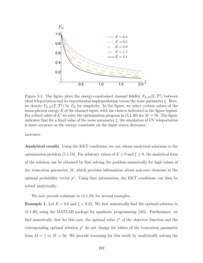
Figure 5.1: The figure plots the energy-constrained channel fidelity FE ,M( I , T

ξ) between

ideal teleportation and its experimental implementation versus the noise parameter ξ . Here,

we denote FE ,M( I , T

ξ) by FE

for simplicity. In the figure, we select certain values of the

mean-photon energy E of the channel input, with the choices indicated in the figure legend.

For a fixed value of E , we solve the optimization program in (5.1.30) for M = 50 . The figure

indicates that for a fixed value of the noise parameter ξ , the simulation of CV teleportation

is more accurate as the energy constraint on the input states decreases.

increases.

Analytical results . Using the KKT conditions, we can obtain analytical solutions to the

optimization problem (5.1.19). For arbitrary values of E ≥ 0 and ξ ≥ 0 , the analytical form

of the solution can be obtained by first solving the problem numerically for high values of

the truncation parameter M , which provides information about non-zero elements in the

optimal probability vector p∗. Using that information, the KKT conditions can then be

solved analytically.

We now provide solutions to (5.1.19) for several examples.

Example 1 . Let E = 0 . 6 and ξ = 0 . 25 . We first numerically find the optimal solution to

(5.1.30) using the MATLAB package for quadratic programming [165]. Furthermore, we

find numerically that for this case, the optimal value f

∗ of the objective function and the

corresponding optimal solution p∗ do not change for values of the truncation parameter

from M = 1 to M = 50 . We provide reasoning for this result by analytically solving the

192

quadratic program by invoking the KKT conditions.

We now analytically find primal and dual feasible points that satisfy the KKT condi-

tions and hence the optimal solution to (5.1.19) for E = 0 . 6 and ξ = 0 . 25 . We begin by

presenting the KKT conditions for the optimization problem in (5.1.19).

Stationarity ∂p

L ( p, µ, β , γ ) |p = p∗ = 0

Primal feasibility

∑

n

np∗

n

− E ≤ 0

p∗

n

≥ 0 , ∀ n ∈ Z≥ 0

∑

n

p∗

n

= 1

Dual feasibility µ ≥ 0

βn

≥ 0 , ∀ n ∈ Z≥ 0

Complementary slackness µ (∑

n

np∗

n

− E ) = 0

βn

p∗

n

= 0 , ∀ n ∈ Z≥ 0

(5.1.37)

We find a set (˜ p, ˜ µ, β , ˜ γ ) that satisfies the KKT conditions, which further implies that

˜ p = p∗ and f

∗ = f ( p∗) , where f ( p ) is defined in (5.1.19). Let ˜ pn

= 0 , ∀ n ≥ 2 . Let us

suppose that the mean energy constraint is saturated, i.e., ˜ p1

= E , which satisfies one

of the complementary slackness conditions. To satisfy βn˜ pn

= 0 , for n = 0 , 1 , we set

β0

= β1

= 0 . From the primal feasibility condition, we get ˜ p0

= 1 − ˜ p1

= 1 − E . All we

need to show now is that µ ≥ 0 and βn

≥ 0 , ∀ n ≥ 2 . Combining all these facts will imply

that the KKT conditions are satisfied. First, to simplify the calculation, we define

G ( n, m, ξ ) =

min n,m ∑

k =0

(n

k

)(m

k

)

ξ2 k

(1 + ξ )n + m +1

.

(5.1.38)

Then from the stationarity condition ˜ p0

and ˜ p1, we get the following linear system of

193

equations:

2 G (0 , 0 , ξ )˜ p0

+ 2 G (1 , 0 , ξ )˜ p1

+ γ = 0 , (5.1.39)

2 G (0 , 1 , ξ )˜ p0

+ 2 G (1 , 1 , ξ )˜ p1

+ µ + γ = 0 . (5.1.40)

By solving for µ and γ , we find [165]

µ =

2 ξ (1 − (2 E − 1) ξ )

(1 + ξ )3

> 0 , (5.1.41)

γ = −2(1 + (1 − E ) ξ )

(1 + ξ )2

, (5.1.42)

for E = 0 . 6 and ξ = 0 . 25 .

Since µ > 0 , in order to satisfy all the KKT conditions for (5.1.19), we only need to

show that βn

≥ 0 , ∀ n ≥ 2 . From the stationarity condition for ˜ pn

we get

βn

= 2 G (0 , n, ξ )˜ p0

+ 2 G (1 , n, ξ )˜ p1

+ nµ + γ .

(5.1.43)

The only negative term in (5.1.43) is γ . For this example we get µ = 0 . 2432 and γ =

− 1 . 408 . Since − γ /µ = 5 . 79 , we get nµ ≥ − γ , ∀ n ≥ 6 . This further implies that βn

≥ 0 ,

∀ n ≥ 6 . Moreover, we solve for β2

, β3, β4, and β5

using (5.1.43) and find their values to

be 0 . 041 , 0 . 1160 , 0 . 2202 , and 0 . 348 , respectively [165]. Thus we get βn

≥ 0 , ∀ n ≥ 2 . This

completes the proof.

Since all the KKT conditions are satisfied and since f ( p ) is a convex function, we

conclude that ˜ p is the optimal solution, i.e., ˜ p = p∗ = (1 − E , E , 0 , . . . , 0) and the optimal

objective function value is given by

f

∗ = f ( p∗) =

1 + ξ (2 + ξ − 2 E (1 + (1 − E ) ξ ))

(1 + ξ )3

= 0 . 6310 ,

(5.1.44)

194

for E = 0 . 6 and ξ = 0 . 25 , which is equal to the optimal value obtained numerically.

Furthermore, for this case, the optimal state corresponding to the channel fidelity between

the ideal teleportation and its experimental approximation is given by

| ψ ⟩R A

=

√

1 − E | 0 ⟩A

| 0 ⟩R

+

√

E | 1 ⟩A

| 1 ⟩R

.

(5.1.45)

Example 2 . Let us consider the case when E = 1 . 2 and ξ = 2 / 3 . Numerically, we find that

the optimal solution has ˜ pn

= 0 , ∀ n , except for n = 0 , 1 , 2 . To satisfy the complementary

slackness condition, we set β0

= β1

= β2

= 0 . Similar to the previous case, we assume that

the energy constraint is satisfied, i.e., ˜ p1 +2˜ p2

= E . By invoking the stationarity conditions

for ˜ p0

, ˜ p1, and ˜ p2, and the primal feasibility condition and by solving the linear system of

equations, we get that [165]

˜ p0

=

ξ (5 ξ + 3 E (1 − ξ ) − 2) − 1

6 ξ2

> 0 , (5.1.46)

˜ p1

=

1 + ξ (2 − 3 E + ξ )

3 ξ2

≥ 0 , (5.1.47)

˜ p2

=

(1 + ξ )( ξ (3 E − 1) − 1)

6 ξ2

> 0 , (5.1.48)

µ =

ξ (1 + (1 − E ) ξ )

(1 + ξ )3

> 0 , (5.1.49)

γ = −5 + (5 − 3 E ) ξ

3(1 + ξ )2

, (5.1.50)

for E = 1 . 2 and ξ = 2 / 3 . Moreover, similar to the previous case, we find that βn

≥ 0 , ∀ n ≥ 3

[165].

Since all the KKT conditions are satisfied and since f ( p ) is a convex function, we

conclude that ˜ p is the optimal solution, i.e., ˜ p = p∗. Moreover, the optimal objective

function is given by

f

∗ = f ( p∗) =

5 + 5 ξ (2 + ξ ) − 3 E ξ (2 + (2 − E ) ξ )

6(1 + ξ )3

,

(5.1.51)

195

and the corresponding optimal state to distinguish the ideal teleportation channel from its

experimental approximation is

| ψ ⟩R A

=

√

˜ p0

| 0 ⟩A

| 0 ⟩R

+

√

˜ p1

| 1 ⟩A

| 1 ⟩R

+

√

˜ p2

| 2 ⟩A

| 2 ⟩R

.

(5.1.52)

Example 3 . We provide an analytical solution for another interesting example when ξ

is close to zero, which corresponds to the case of the additive-noise channel converging to

the ideal teleportation channel. This example is experimentally relevant, as the goal of an

approximate teleportation protocol is to converge to the ideal teleportation channel. In

such a scenario we argue that

| ψ ⟩R A

=

√

1 − E |⌊ E ⌋⟩A

|⌊ E ⌋⟩R

+

√

E |⌈ E ⌉⟩A

|⌈ E ⌉⟩R

(5.1.53)

is the optimal state for the optimization problem in (5.1.1), where E = E − ⌊ E ⌋ . More-

over, the minimum fidelity in (5.1.1) is given by

FE( IA

, T

ξ

A) = (1 − E )2 G ( ⌊ E ⌋ , ⌊ E ⌋ , ξ ) + 2 E (1 − E ) G ( ⌊ E ⌋ , ⌈ E ⌉ , ξ )

+ ( E )2 G ( ⌈ E ⌉ , ⌈ E ⌉ , ξ ) , (5.1.54)

where G ( n, m, ξ ) is defined in (5.1.38).

Since the marginal of the state | ψ ⟩R A

in (5.1.53) has energy Tr(ˆ nψA) = E , one of the

complementary slackness conditions is satisfied. Let us suppose that p∗

n

= 0 , ∀ n , except

for n = ⌊ E ⌋ and ⌈ E ⌉ . Therefore, p∗

⌊ E ⌋

= 1 − E and p∗

⌈ E ⌉

= E , which implies that

β⌊ E ⌋

= β⌈ E ⌉

= 0 , to satisfy the other complementary slackness conditions. Similar to the

previous examples, we need to solve the following linear system of equations and show that

196

µ ≥ 0 when ξ is close to zero:

2 p∗

⌊ E ⌋

G ( ⌊ E ⌋ , ⌊ E ⌋ , ξ ) + 2 p∗

⌈ E ⌉

G ( ⌊ E ⌋ , ⌈ E ⌉ , ξ ) + ⌊ E ⌋ µ + γ = 0 , (5.1.55)

2 p∗

⌈ E ⌉

G ( ⌈ E ⌉ , ⌈ E ⌉ , ξ ) + 2 p∗

⌊ E ⌋

G ( ⌊ E ⌋ , ⌈ E ⌉ , ξ ) + ⌈ E ⌉ µ + γ = 0 . (5.1.56)

By solving for µ , we get

µ = 2

(

p∗

⌊ E ⌋( G ( ⌊ E ⌋ , ⌊ E ⌋ , ξ ) − G ( ⌊ E ⌋ , ⌈ E ⌉ , ξ )) + p∗

⌈ E ⌉( G ( ⌊ E ⌋ , ⌈ E ⌉ , ξ ) − G ( ⌈ E ⌉ , ⌈ E ⌉ , ξ ))

)

,

(5.1.57)

≈ 2 ξ + O ( ξ2) , (5.1.58)

which implies that the leading order term 2 ξ ≥ 0 for any finite value of the energy con-

straint E . Similarly, we find that

βn

≈ ( ⌊ E ⌋ − n )( ⌈ E ⌉ − n ) ξ2 + O ( ξ3) , ∀ n, (5.1.59)

where again the leading term implies that βn

≥ 0 when ξ is close to zero. By combining

everything, we conclude that all the KKT conditions are satisfied. Hence, for ξ close to

zero, the state in (5.1.53) is optimal for the task of distinguishing the ideal teleportation

channel from its experimental approximation when there is a finite energy constraint on

the input states to the channels.

Finally, we consider several experimentally relevant quantum states with energy con-

straints, such as coherent states and the two-mode squeezed vacuum state (TMSV).

Example 4 . Let | α ⟩ denote a coherent state and let E = | α |2. We note that the covariance

matrix of a coherent state is a two-dimensional identity matrix, which under an additive-

noise channel T

ξ becomes VT

ξ( | α ⟩⟨ α | )

= diag (1 + 2 ξ ) . Then the fidelity between | α ⟩ and

197

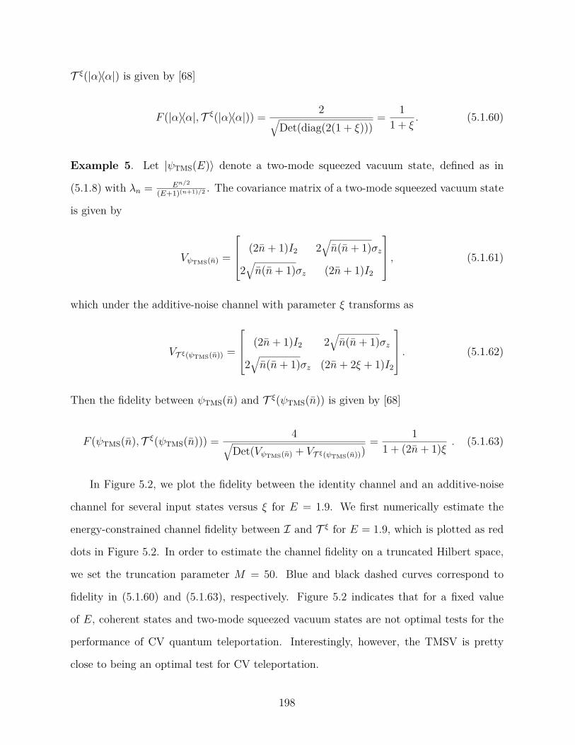
T

ξ( | α ⟩⟨ α | ) is given by [68]

F ( | α ⟩⟨ α | , T

ξ( | α ⟩⟨ α | )) =

2

√

Det ( diag (2(1 + ξ )))

=

1

1 + ξ

.

(5.1.60)

Example 5 . Let | ψTMS( E ) ⟩ denote a two-mode squeezed vacuum state, defined as in

(5.1.8) with λn

=

E

n/ 2

( E +1)( n +1) / 2 . The covariance matrix of a two-mode squeezed vacuum state

is given by

VψTMS(¯ n )

=

(2¯ n + 1) I2

2

√

¯ n (¯ n + 1) σz

2

√

¯ n (¯ n + 1) σz

(2¯ n + 1) I2

, (5.1.61)

which under the additive-noise channel with parameter ξ transforms as

VT

ξ( ψTMS(¯ n ))

=

(2¯ n + 1) I2

2

√

¯ n (¯ n + 1) σz

2

√

¯ n (¯ n + 1) σz

(2¯ n + 2 ξ + 1) I2

.

(5.1.62)

Then the fidelity between ψTMS(¯ n ) and T

ξ( ψTMS(¯ n )) is given by [68]

F ( ψTMS(¯ n ) , T

ξ( ψTMS(¯ n ))) =

4

√

Det ( VψTMS(¯ n )

+ VT

ξ( ψTMS(¯ n )))

=

1

1 + (2¯ n + 1) ξ

.

(5.1.63)

In Figure 5.2, we plot the fidelity between the identity channel and an additive-noise

channel for several input states versus ξ for E = 1 . 9 . We first numerically estimate the

energy-constrained channel fidelity between I and T

ξ for E = 1 . 9 , which is plotted as red

dots in Figure 5.2. In order to estimate the channel fidelity on a truncated Hilbert space,

we set the truncation parameter M = 50 . Blue and black dashed curves correspond to

fidelity in (5.1.60) and (5.1.63), respectively. Figure 5.2 indicates that for a fixed value

of E , coherent states and two-mode squeezed vacuum states are not optimal tests for the

performance of CV quantum teleportation. Interestingly, however, the TMSV is pretty

close to being an optimal test for CV teleportation.

198

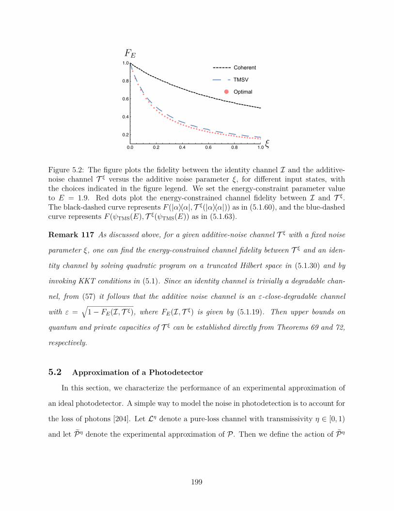
Optimal

TMSV

Coherent

Figure 5.2: The figure plots the fidelity between the identity channel I and the additive-

noise channel T

ξ versus the additive noise parameter ξ , for different input states, with

the choices indicated in the figure legend. We set the energy-constraint parameter value

to E = 1 . 9 . Red dots plot the energy-constrained channel fidelity between I and T

ξ.

The black-dashed curve represents F ( | α ⟩⟨ α | , T

ξ( | α ⟩⟨ α | )) as in (5.1.60), and the blue-dashed

curve represents F ( ψTMS( E ) , T

ξ( ψTMS( E )) as in (5.1.63).

Remark 117 As discussed above, for a given additive-noise channel T

ξ with a fixed noise

parameter ξ , one can find the energy-constrained channel fidelity between T

ξ and an iden-

tity channel by solving quadratic program on a truncated Hilbert space in (5.1.30) and by

invoking KKT conditions in (5.1) . Since an identity channel is trivially a degradable chan-

nel, from (57) it follows that the additive noise channel is an ε -close-degradable channel

with ε =

√

1 − FE( I , T

ξ) , where FE( I , T

ξ) is given by (5.1.19) . Then upper bounds on

quantum and private capacities of T

ξ can be established directly from Theorems 69 and 72,

respectively.

5.2 Approximation of a Photodetector

In this section, we characterize the performance of an experimental approximation of

an ideal photodetector. A simple way to model the noise in photodetection is to account for

the loss of photons [204]. Let Lη denote a pure-loss channel with transmissivity η ∈ [0 , 1)

and let P

η denote the experimental approximation of P . Then we define the action of P

η

199

on a density operator ρ as follows:

P

η( ρ ) ≡ P Lη( ρ ) ,

(5.2.1)

where P is defined in (2.3.90).

Energy-constrained diamond distance between P and P

η. We now evaluate the

energy-constrained diamond distance between P

η and P . We first summarize the main

results and subsequently provide detailed proof steps.

Employing the joint phase covariance of P and P

η, it follows that among all pure

states, entangled superpositions of twin-Fock states, as defined in (5.1.8), are optimal to

distinguish P from P with respect to the energy-constrained diamond distance.

Let E ≡ E − ⌊ E ⌋ . Then from the direct-sum property of the trace distance on

classical-quantum states and convexity of the function x → η

x, where η ∈ [0 , 1) , we find

that

1

2

∥P − P

η ∥⋄ E

= 1 −

[

(1 − E ) η

⌊ E ⌋ + E η

⌈ E ⌉

]

.

(5.2.2)

Moreover, a state that optimizes the energy-constrained diamond distance in (5.2.2) is

given by the following mixed number state:

ψA

= (1 − E ) |⌊ E ⌋⟩⟨⌊ E ⌋|A

+ E |⌈ E ⌉⟩⟨⌈ E ⌉|A

.

(5.2.3)

From (5.2.3) it follows that entanglement is not necessary to attain the optimal distin-

guishability of the ideal photodetector P from its experimental approximation P

η. We

now provide a detailed proof.

Proof of (5.2.2) and (5.2.3) . Our goal is to estimate the trace distance between ( IR

⊗

PA)( ψR A) and ( IR

⊗ P

η

A)( ψR A) , where ψR A


Let

g ( n, m, η ) =

√√√√

(n

k

)(m

k

)

η

n + m − 2 k(1 − η )2 k .

(5.2.4)

200

Consider the following chain of equalities:

∥∥∥ ( IR

⊗ PA)( ψR A) − ( IR

⊗ P

η

A)( ψR A)

∥∥∥1

= ∥ ( IR

⊗ PA)( ψR A) − ( IR

⊗ ( PA

Lη

A))( ψR A) ∥1

(5.2.5)

=

∥∥∥∥∥∥

∞∑

n,m =0

λm

λn

| n ⟩⟨ m |R

⊗

P ( | n ⟩⟨ m |A) −

min n,m ∑

k =0

g ( n, m, η ) P ( | n − k ⟩⟨ m − k |A)

∥∥∥∥∥∥1

(5.2.6)

=

∥∥∥∥∥

∞∑

n =0

λ2

n

| n ⟩⟨ n |R

⊗

[

| n ⟩⟨ n |A

−

n∑

k =0

(n

k

)

η

k(1 − η )n − k | k ⟩⟨ k |A

]∥∥∥∥∥

1

(5.2.7)

=

∞∑

n =0

λ2

n

∥∥∥∥∥| n ⟩⟨ n |A

−

n∑

k =0

(n

k

)

η

k(1 − η )n − k | k ⟩⟨ k |A)

∥∥∥∥∥

1

(5.2.8)

=

∞∑

n =0

λ2

n

[n − 1∑

k =0

(n

k

)

η

k(1 − η )n − k + 1 − η

n

]

(5.2.9)

= 2

(

1 −

∞∑

n =0

λ2

n

η

n

)

. (5.2.10)

The second equality follows from the action of a pure-loss channel on a number state. The

third equality follows from (2.3.90). The fourth equality is a consequence of the direct-sum

property the trace distance on classical-quantum states. The rest of the steps follow from

basic algebraic manipulations.

Therefore, the energy-constrained diamond distance between P and P

η reduces to the

following optimization problem:

1

2

∥P − P

η ∥⋄ E

= max

λ2n

n:∑

n

λ2n=1 ,

∑

n

nλ2n

≤ E

(

1 −

∞∑

n =0

λ2

n

η

n

)

.

(5.2.11)

The optimization in (5.2.11) can be solved by following a method introduced in [186].

We provide a proof for completeness. Suppose that

∑

n

nλ2

n

= F , Al

=

∑⌊ F ⌋

n =0

λ2

n

, Au

=

201

∑∞

n = ⌈ F ⌉

λ2

n, Fl

=

∑⌊ F ⌋

n =0( λ2

n

/Al) n , and Fu

=

∑∞

n = ⌈ E ⌉( λ2

n

/Au) n . Then it follows that

Al

+ Au

= 1 , (5.2.12)

F = Al

Fl

+ Au

Fu

, (5.2.13)

Fl

≤ ⌊ F ⌋ , (5.2.14)

Fu

≥ ⌈ F ⌉ . (5.2.15)


∞∑

n =0

λ2

n

η

n = Al

⌊ F ⌋∑

n =0

λ2

n

Al

η

n + Au

∞∑

n = ⌈ F ⌉

λ2

n

Au

η

n (5.2.16)

≥ Al

η

Fl + Au

η

Fu (5.2.17)

≥ λ2

⌊ F ⌋

η

⌊ F ⌋ + λ2

⌈ F ⌉

η

⌈ F ⌉ (5.2.18)

= (1 − F ) η

⌊ F ⌋ + F η

⌈ F ⌉ . (5.2.19)

where the first inequality follows from the convexity of the function x → η

x. The last

inequality follows from the fact that the chord joining ( ⌊ F ⌋ , η

⌊ F ⌋) and ( ⌈ F ⌉ , η

⌈ F ⌉) is below

the chord joining ( Al

, η

Fl) and ( Au

, η

Fu) due to the convexity of the function. Moreover,

the energy of the initial state can be satisfied by taking Fl

= ⌊ F ⌋ and Fu

= ⌈ F ⌉ , and the

corresponding probability elements are given by λ2

⌊ F ⌋

= 1 − F and λ2

⌈ F ⌉

= F .

Since (5.2.19) monotonically decreases with F , it implies that the solution to the op-

timization problem in (5.2.11) is given by a state that saturates the energy constraint.

Therefore, the optimal state is given by (5.2.3). This completes the proof of (5.2.2).

Numerical results . Next, we perform numerical evaluations to analyze the accuracy in

202

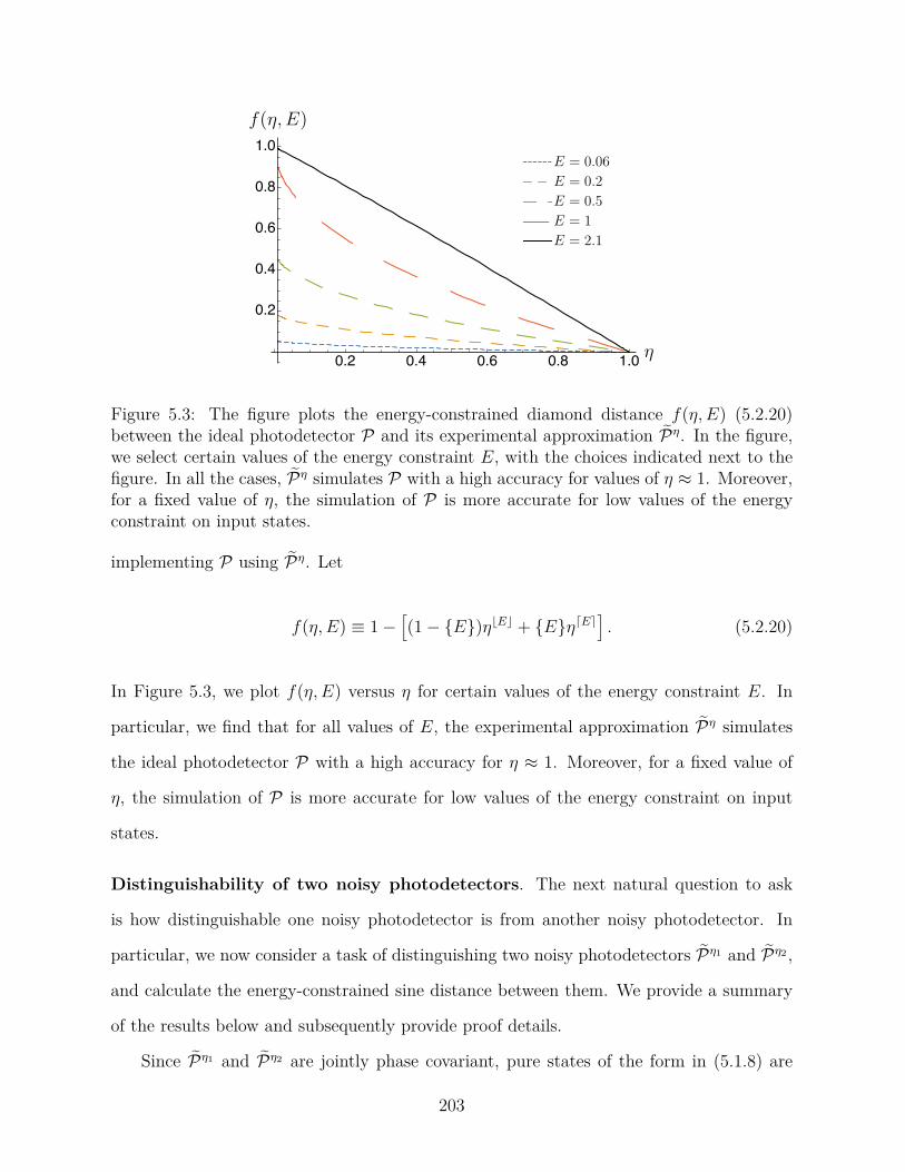
Figure 5.3: The figure plots the energy-constrained diamond distance f ( η , E ) (5.2.20)

between the ideal photodetector P and its experimental approximation P

η. In the figure,

we select certain values of the energy constraint E , with the choices indicated next to the

figure. In all the cases, P

η simulates P with a high accuracy for values of η ≈ 1 . Moreover,

for a fixed value of η , the simulation of P is more accurate for low values of the energy

constraint on input states.

implementing P using P

η. Let

f ( η , E ) ≡ 1 −

[

(1 − E ) η

⌊ E ⌋ + E η

⌈ E ⌉

]

.

(5.2.20)

In Figure 5.3, we plot f ( η , E ) versus η for certain values of the energy constraint E . In

particular, we find that for all values of E , the experimental approximation P

η simulates

the ideal photodetector P with a high accuracy for η ≈ 1 . Moreover, for a fixed value of

η , the simulation of P is more accurate for low values of the energy constraint on input

states.

Distinguishability of two noisy photodetectors . The next natural question to ask

is how distinguishable one noisy photodetector is from another noisy photodetector. In

particular, we now consider a task of distinguishing two noisy photodetectors P

η1 and P

η2 ,

and calculate the energy-constrained sine distance between them. We provide a summary

of the results below and subsequently provide proof details.

Since P

η1 and P

η2 are jointly phase covariant, pure states of the form in (5.1.8) are

203

optimal to distinguish them with respect to the energy-constrained sine distance. We then

find that

CE( P

η1 , P

η2) =

√

1 − [(1 − E ) µ⌊ E ⌋ + E µ⌈ E ⌉]2

, (5.2.21)

where E ≡ E − ⌊ E ⌋ and µ ≡

√

η1

η2

+

√

(1 − η1)(1 − η2) . Moreover, the state that

optimizes the energy-constrained sine distance in (5.2.21) is given by (5.2.3), which again

implies that entanglement is not necessary for the optimal distinguishability of two noisy

photodetectors.

Proof for (5.2.21). First note that the output of a noisy photodetector P

η when the input

state is ψR A

in (5.1.8) is given by

P

η( ψR A) = ( P Lη)( ψR A) (5.2.22)

=

∑

n

n∑

k =0

β ( λn

, η , k ) | n ⟩⟨ n |R

⊗ | k ⟩⟨ k |A

, (5.2.23)

where

β ( λn

, η , k ) = λ2

n

(n

k

)

η

k

1(1 − η1)n − k (5.2.24)

are the eigenvalues of P

η( ψR A) . Therefore, the fidelity between P

η1( ψR A) and P

η2( ψR A) is

204

given by

F ( P

η1( ψR A) , P

η2( ψR A)) =

[

Tr

(√

√

P

η1( ψR A) P

η2( ψR A)

√

P

η1( ψR A)

)]2

(5.2.25)

=

[∑

n

n∑

k =0

√

β ( λn

, η1

, k ) β ( λn

, η2

, k )

]2

(5.2.26)

=

[∑

n

λ2

n

n∑

k =0

(n

k

)√

η1

η2

k

[

(1 − η1)(1 − η2)

]n − k

]2

(5.2.27)

=

[∑

n

λ2

n

(√

η1

η2

+

√

(1 − η1)(1 − η2)

)n

]2

(5.2.28)

=

[∑

n

λ2

n

µn

]2

, (5.2.29)

where

µ =

√

η1

η2

+

√

(1 − η1)(1 − η2) . (5.2.30)

Then from [190], we find that the energy-constrained sine distance between P

η1 and

P

η2 is given by

CE( P

η1 , P

η2) =

√

1 − [(1 − E ) µ⌊ E ⌋ + E µ⌈ E ⌉]2

, (5.2.31)

where E = E − ⌊ E ⌋ . Moreover, the state that optimizes the energy-constrained sine

distance in (5.2.21) is given by (5.2.3), which proves that entanglement is not necessary for

the optimal distinguishability of two noisy photodetectors.

5.3 Conclusion

In this chapter, using energy-constrained distinguishability measures, we quantified the

accuracy in implementing continuous-variable (CV) quantum teleportation and a photode-

tector.

CV teleportation . We proposed an optimal test to characterize the performance of CV

205

teleportation in terms of the energy-constrained channel fidelity between ideal CV telepor-

tation and its experimental approximation. We reduced the optimization problem of esti-

mating the energy-constrained channel fidelity to a quadratic program with inequality con-

straints. Since, in general, optimization over an infinite number of variables is not possible,

we defined the energy-constrained channel fidelity on a truncated Hilbert space, which re-

duces to a truncated version of the quadratic program with inequality constraints. We then

showed that the objective function of the quadratic program is convex. As a consequence

of the linearity of the inequality constraints and the convexity of the objective function, we

found analytical solutions to the quadratic program by invoking the Karush–Kuhn–Tucker

conditions. We then proved that these solutions to the energy-constrained channel fidelity

on a truncated Hilbert space also optimize the energy-constrained channel fidelity defined

over an infinite-dimensional separable Hilbert space.

Prior to our results, the accuracy in implementing CV teleportation was quantified

by considering several input states, such as ensembles of coherent states, squeezed states,

cat states, etc. We showed that instead, entangled superpositions of twin-Fock states are

optimal to characterize the performance of CV teleportation. Thus, our result provides

a benchmark for teleporting an unknown, energy-constrained state using CV quantum

teleportation. Another interesting metric to quantify the accuracy in simulating ideal CV

teleportation is the energy-constrained diamond distance between ideal CV teleportation

and its experimental approximation. We leave the calculation of this quantity for future

work.

Photodetectors . In this chapter, we also analytically calculated the energy-constrained

diamond distance between the ideal photodetector and its experimental approximation.

We modeled the noise in the experimental approximation of a photodetector as a pure-loss

channel. Our main result here is that entanglement with a reference system is not required

to quantify the accuracy in implementing a photodetector and the optimal input state is a

mixture of photon number states. It is an interesting open question to determine the opti-

206

mal value of the energy-constrained distance measures when the noise in a photodetector

is modeled as a thermal noise channel.

207

CHAPTER 6

CONCLUSION AND OPEN QUESTIONS

In this dissertation, we extensively studied several applications of energy-constrained

distinguishability measures. Our results apply broadly to communication and computation

tasks using continuous-variable quantum resources. In particular, we established several

upper bounds on the quantum and private capacities of phase-insensitive, bosonic Gaussian

channels. We described the importance of energy-constrained distinguishability measures

by showing that bounds based on the approximate degradability of quantum channels can

be tighter than all other upper bounds on capacities. We then studied applications of

energy-constrained distance measures in assessing the performance of continuous-variable

Gaussian logic gates. As a final application of energy-constrained distinguishability mea-

sures, we solved an open problem related to benchmarking CV quantum teleportation.

We proved that the optimal state to distinguish ideal teleportation from its experimental

approximation with respect to the energy-constrained channel fidelity is an entangled super-

position of twin-Fock states. Thus our results quantify the worst-case error in teleporting

a quantum state using CV quantum resources.

Below we summarize our results and several open problems.

Optimal rate of communication . In Chapter 3 we established several upper bounds

on the ultimate rate of quantum and private communication using thermal, amplifier, and

additive-noise channels. In particular, two upper bounds are based on the approximate

degradability of quantum channels. These bounds depend on the energy-constrained dis-

tance between two particular Gaussian channels. Therefore, tighter bounds on capacities

can be established by finding better estimates of the energy-constrained diamond distance

between particular Gaussian channels. We now summarize open problems in the context

of communication using bosonic Gaussian resources:

• As discussed in Chapters 3–5, in general, estimating the energy-constrained channel

208

divergences is a computationally challenging problem. Although we have developed

numerical and analytical techniques in Chapters 4 and 5 to find good estimates of

energy-constrained sine and diamond distances, it is not straightforward to apply

these techniques to find approximate-degradable upper bounds on capacities. It is

an interesting open question to further tighten approximate-degradable bounds on

capacities of phase-insensitive Gaussian channels.

• Other ways to establish bounds on capacities of non-degradable quantum chan-

nels is to use notions of approximate anti-degradability, approximate entanglement-

breakability, and approximate covariance (see [98] for a review on these techniques).

Bounds based on these techniques also rely on the energy-constrained channel di-

vergences between two particular Gaussian channels. Thus it is interesting to study

these techniques for bounding capacities of CV Gaussian channels.

• In Chapter 3 we considered the communication setting where an infinite number of

channel uses was allowed. It is an interesting open question to develop the notion

of communication over bosonic Gaussian channels with energy constraints such that

only a finite number of channel uses is allowed.

Continuous-variable quantum logic gates . In Chapter 4, we studied several notions of

convergence for quantum channels. We then estimated the energy-constrained sine distance

between ideal Gaussian unitaries and their experimental implementations. Our results

imply that as the energy constraint on the input states to the channels increases, the

accuracy in experimentally implementing a Gaussian unitary transformation decreases.

There are several open research questions on this topic, summarized below.

• There are limitations to problems that can be solved using methods introduced in

this dissertation. For example, we could estimate the energy-constrained sine distance

between an ideal displacement and its experimental implementation. On the other

209

hand, it is still an open question to determine the energy-constrained sine distance

between the ideal online squeezing operation and its experimental implementation.

Similarly, we could only estimate the distance between an ideal SUM gate and its

experimental implementation for a particular input state. Hence the problem of

estimating the energy-constrained sine or diamond distance between the ideal SUM

gate and its experimental implementation is still open.

• Other Gaussian operations of interest are homodyne and heterodyne measurements.

It is an open problem to estimate the accuracy in implementing these operations.

• In Chapter 4, we studied only optical implementations of several Gaussian unitaries.

It will be interesting to perform a similar study to quantify the accuracy in imple-

menting Gaussian operations on other platforms such as vibrational modes of trapped

ions [205] and microwave circuits [206].

• Another interesting direction is to use these results to study the error propagation in

an experiment based on Gaussian unitaries.

• In this dissertation, we invoked properties of Gaussian unitaries and channels in order

to solve the optimization involved in several energy-constrained channel divergences.

It is an open problem to develop techniques to study the accuracy in implementing

non-Gaussian unitaries.

Continuous-variable quantum teleportation . In Chapter 5, we proposed an optimal

test to assess the performance of CV teleportation. In particular, we developed numerical

and analytical methods to evaluate the energy-constrained channel fidelity between ideal

CV teleportation and its experimental implementation. We now list some open problems

related to CV teleportation:

• Is it possible to evaluate the energy-constrained diamond distance between CV tele-

portation and its experimental implementation? Using solutions of the quadratic

210

program in (5.1.19) and from (2.4.20), we get bounds on the energy-constrained

diamond distance between CV teleportation and its experimental implementation.

Results of a similar spirit appeared recently in [91].

• How does the accuracy in implementing CV teleportation affect other applications

where CV teleportation is used, such as error correction, quantum networks, and

quantum key distribution?

Optimization problems . In this dissertation, we solved several optimization problems.

• As summarized in Remark 79, any energy-constrained optimization problem – with

optimization over quantum states – based on quantum channels would have thermal-

state input saturating the energy constraint as an optimal input state if the following

conditions hold: 1) The objective function being optimized is invariant with respect

to local unitaries and concave in the input state. 2) The channel is phase and dis-

placement covariant. It will be interesting to find further applications of this result.

• Similarly, in Section 3.8, we solved a general Gaussian optimization problem, where

we showed that for two Gaussian channels that are jointly phase and displacement

covariant, the Gaussian energy-constrained generalized channel divergence is achieved

by a two-mode squeezed vacuum state that saturates the energy constraint. An

interesting question to answer is for which Gaussian channels the two-mode squeezed

vacuum state that saturates the energy constraint is an optimal state among all states

for several energy-constrained, generalized channel divergences.

• In Chapter 4 (see Eq. (4.1.67)), we presented a semidefinite program to estimate the

energy-constrained diamond distance between two channels on a truncated infinite-

dimensional separable Hilbert space. Similarly, in Chapter 5 (see Eq. (5.1.30)) we

estimated the energy-constrained channel fidelity between two particular Gaussian

channels by first solving a quadratic program on a truncated Hilbert space and then

211

by invoking KKT conditions. It will be interesting to find further examples where

these techniques can be directly used.

212

REFERENCES

[1] Michael A. Nielsen and Isaac L. Chuang. Quantum Computation and Quantum In-

formation: 10th Anniversary Edition . Cambridge University Press, Cambridge, UK,

2010.

[2] Daniel R. Simon. On the power of quantum computation. SIAM Journal on Com-

puting , 26(5):1474–1483, October 1997.

[3] Peter W. Shor. Polynomial-time algorithms for prime factorization and discrete log-

arithms on a quantum computer. SIAM Review , 41(2):303–332, 1999.

[4] Michel Boyer, Gilles Brassard, Peter Høyer, and Alain Tapp. Tight bounds on quan-

tum searching. Fortschritte der Physik: Progress of Physics , 46(4-5):493–505, April

1999. arXiv:quant-ph/9605034.

[5] Dave Wecker, Matthew B. Hastings, Nathan Wiebe, Bryan K. Clark, Chetan Nayak,

and Matthias Troyer. Solving strongly correlated electron models on a quantum

computer. Physical Review A , 92:062318, December 2015. arXiv:1506.05135.

[6] Dave Wecker, Bela Bauer, Bryan K. Clark, Matthew B. Hastings, and Matthias

Troyer. Gate-count estimates for performing quantum chemistry on small quantum

computers. Physical Review A , 90:022305, August 2014. arXiv:1312.1695.

[7] Stephen P. Jordan, Keith SM Lee, and John Preskill. Quantum algorithms for quan-

tum field theories. Science , 336(6085):1130–1133, June 2012. arXiv:1111.3633.

[8] Mark M. Wilde. Quantum Information Theory . Cambridge University Press, 2nd

edition, 2017. arXiv:1106.1445v7.

[9] Charles H. Bennett and Gilles Brassard. Quantum cryptography: Public key distri-

bution and coin tossing. Theoretical Computer Science , 560(1):7–11, December 2020.

arXiv:2003.06557.

[10] Peter W. Shor and John Preskill. Simple proof of security of the bb84 quantum key

distribution protocol. Physical Review Letters , 85:441–444, July 2000. arXiv:quant-

ph/0003004.

[11] Charles H. Bennett, Gilles Brassard, Claude Crépeau, Richard Jozsa, Asher Peres,

and William K. Wootters. Teleporting an unknown quantum state via dual classical

and Einstein-Podolsky-Rosen channels. Physical Review Letters , 70(13):1895, March

1993.

[12] Michael A. Nielsen, Emanuel Knill, and Raymond Laflamme. Complete quantum

teleportation using nuclear magnetic resonance. Nature , 396(6706):52–55, November


213

https://arxiv.org/abs/quant-ph/9605034

https://arxiv.org/abs/1506.05135








[13] Olivier Landry, J. A. W. van Houwelingen, Alexios Beveratos, Hugo Zbinden, and

Nicolas Gisin. Quantum teleportation over the Swisscom telecommunication net-

work. Journal of the Optical Society of America B , 24(2):398–403, February 2007.

arXiv:quant-ph/0605010.

[14] Xiao-Song Ma, Thomas Herbst, Thomas Scheidl, Daqing Wang, Sebastian

Kropatschek, William Naylor, Bernhard Wittmann, Alexandra Mech, Johannes

Kofler, Elena Anisimova, et al. Quantum teleportation over 143 kilometres using

active feed-forward. Nature , 489(7415):269–273, September 2012. arXiv:1205.3909.

[15] Xiao-Hui Bao, Xiao-Fan Xu, Che-Ming Li, Zhen-Sheng Yuan, Chao-Yang Lu, and

Jian-Wei Pan. Quantum teleportation between remote atomic-ensemble quantum

memories. Proceedings of the National Academy of Sciences , 109(50):20347–20351,

December 2012. arXiv:1211.2892.

[16] Shuntaro Takeda, Takahiro Mizuta, Maria Fuwa, Peter Van Loock, and Akira Fu-

rusawa. Deterministic quantum teleportation of photonic quantum bits by a hybrid

technique. Nature , 500(7462):315–318, August 2013. arXiv:1402.4895.

[17] Christian Nölleke, Andreas Neuzner, Andreas Reiserer, Carolin Hahn, Gerhard

Rempe, and Stephan Ritter. Efficient teleportation between remote single-atom quan-

tum memories. Physical Review Letters , 110(14):140403, April 2013. arXiv:1212.3127.

[18] Benjamin J. Metcalf, Justin B. Spring, Peter C. Humphreys, Nicholas Thomas-Peter,

Marco Barbieri, W. Steven Kolthammer, Xian-Min Jin, Nathan K. Langford, Dmytro

Kundys, James C. Gates, et al. Quantum teleportation on a photonic chip. Nature

Photonics , 8(10):770–774, September 2014. arXiv:1409.4267.

[19] Wolfgang Pfaff, Bas J. Hensen, Hannes Bernien, Suzanne B. van Dam, Machiel S.

Blok, Tim H. Taminiau, Marijn J. Tiggelman, Raymond N. Schouten, Matthew

Markham, Daniel J. Twitchen, et al. Unconditional quantum teleportation be-

tween distant solid-state quantum bits. Science , 345(6196):532–535, August 2014.

arXiv:1404.4369.

[20] Xi-Lin Wang, Xin-Dong Cai, Zu-En Su, Ming-Cheng Chen, Dian Wu, Li Li, Nai-

Le Liu, Chao-Yang Lu, and Jian-Wei Pan. Quantum teleportation of multiple de-

grees of freedom of a single photon. Nature , 518(7540):516–519, February 2015.

arXiv:1409.7769.

[21] Stefano Pirandola, Jens Eisert, Christian Weedbrook, Akira Furusawa, and Samuel L.

Braunstein. Advances in quantum teleportation. Nature Photonics , 9(10):641–652,

September 2015. arXiv:1505.07831.

[22] Ji-Gang Ren, Ping Xu, Hai-Lin Yong, Liang Zhang, Sheng-Kai Liao, Juan Yin, Wei-

Yue Liu, Wen-Qi Cai, Meng Yang, Li Li, et al. Ground-to-satellite quantum telepor-

tation. Nature , 549(7670):70–73, August 2017. arXiv:1707.00934.

214











[23] Isaac L. Chuang and Yoshihisa Yamamoto. A simple quantum computer. Physical

Review A , 52(5):3489, November 1995. arXiv:quant-ph/9505011.

[24] Emanuel Knill, Raymond Laflamme, and Gerard J. Milburn. A scheme for effi-

cient quantum computation with linear optics. Nature , 409:46–52, January 2001.


[25] Daniel Gottesman, Alexei Kitaev, and John Preskill. Encoding a qubit in an oscilla-

tor. Physical Review A , 64(1):012310, June 2001. arXiv:quant-ph/0008040.

[26] Pieter Kok, William J. Munro, Kae Nemoto, Timothy C. Ralph, Jonathan P. Dowling,

and Gerard J. Milburn. Linear optical quantum computing with photonic qubits.

Reviews of Modern Physics , 79(1):135, January 2007. arXiv:quant-ph/0512071.

[27] Seth Lloyd and Samuel L. Braunstein. Quantum computation over continuous

variables. Physical Review Letters , 82(8):1784–1787, February 1999. arXiv:quant-

ph/9810082.

[28] Seth Lloyd. Hybrid Quantum computing. In: Braunstein S.L., Pati A.K. (eds) Quan-

tum Information with Continuous Variables . Springer, Dordrecht, 2003.

[29] Peter Van Loock. Optical hybrid approaches to quantum information. Laser &

Photonics Reviews , 5:167, February 2011. arXiv:1002.4788.

[30] Akira Furusawa and Peter Van Loock. Quantum Teleportation and Entanglement:

A Hybrid Approach to Optical Quantum Information Processing . Wiley-VCH, May

2011.

[31] Valerio Scarani, Helle Bechmann-Pasquinucci, Nicolas J. Cerf, Miloslav Dušek, Nor-

bert Lütkenhaus, and Momtchil Peev. The security of practical quantum key distri-

bution. Reviews of Modern Physics , 81:1301–1350, September 2009. arXiv:0802.4155.

[32] Lev Vaidman. Teleportation of quantum states. Physical Review A , 49(2):1473–1476,

February 1994. arXiv:hep-th/9305062.

[33] Susana F. Huelga, Martin B. Plenio, and Joan A. Vaccaro. Remote control of re-

stricted sets of operations: Teleportation of angles. Physical Review A , 65(4):042316,

April 2002. arXiv:quant-ph/0107110.

[34] Susana F. Huelga, Joan A. Vaccaro, Anthony Chefles, and Martin B. Plenio. Quan-

tum remote control: Teleportation of unitary operations. Physical Review A ,

63(4):042303, March 2001. arXiv:quant-ph/0005061.

[35] Satoshi Ishizaka and Tohya Hiroshima. Asymptotic teleportation scheme as a uni-

versal programmable quantum processor. Physical Review Letters , 101(24):240501,


[36] Satoshi Ishizaka and Tohya Hiroshima. Quantum teleportation scheme by select-

ing one of multiple output ports. Physical Review A , 79(4):042306, April 2009.

arXiv:0901.2975.

215

https://arxiv.org/abs/quant-ph/9505011v1








https://arxiv.org/abs/hep-th/9305062





[37] Samuel L. Braunstein and H. J. Kimble. Teleportation of continuous quantum vari-

ables. Physical Review Letters , 80(4):869, January 1998.

[38] Seth Lloyd. Capacity of the noisy quantum channel. Physical Review A , 55(3):1613–

1622, March 1997. arXiv:quant-ph/9604015.

[39] Peter W. Shor. The quantum channel capacity and coherent information. In lecture

notes, MSRI Workshop on Quantum Computation , 2002.

[40] Ning Cai, Andreas Winter, and Raymond W. Yeung. Quantum privacy and quantum

wiretap channels. Problems of Information Transmission , 40(4):318–336, October

2004.

[41] Igor Devetak. The private classical capacity and quantum capacity of a quantum

channel. IEEE Transactions on Information Theory , 51(1):44–55, January 2005.


[42] Igor Devetak and Peter W. Shor. The capacity of a quantum channel for simultaneous

transmission of classical and quantum information. Communications in Mathematical

Physics , 256(2):287–303, June 2005. arXiv:quant-ph/0311131.

[43] Graeme Smith. Private classical capacity with a symmetric side channel and its

application to quantum cryptography. Physical Review A , 78(2):022306, August 2008.

arXiv:0705.3838.

[44] David P. DiVincenzo, Peter W. Shor, and John A. Smolin. Quantum-channel ca-

pacity of very noisy channels. Physical Review A , 57(2):830–839, February 1998.


[45] Graeme Smith and John A. Smolin. Degenerate quantum codes for Pauli channels.

Physical Review Letters , 98(3):030501, January 2007. arXiv:quant-ph/0604107.

[46] Graeme Smith, Joseph M. Renes, and John A. Smolin. Structured codes improve

the Bennett-Brassard-84 quantum key rate. Physical Review Letters , 100(17):170502,

April 2008. arXiv:quant-ph/0607018.

[47] Toby Cubitt, David Elkouss, William Matthews, Maris Ozols, David Pérez-García,

and Sergii Strelchuk. Unbounded number of channel uses are required to see quantum

capacity. Nature Communications , 6:7739, March 2015. arXiv:1408.5115.

[48] David Elkouss and Sergii Strelchuk. Superadditivity of private information for any

number of uses of the channel. Physical Review Letters , 115(4):040501, July 2015.

arXiv:1502.05326.

[49] Graeme Smith and Jon Yard. Quantum communication with zero-capacity channels.

Science , 321(5897):1812–1815, September 2008. arXiv:0807.4935.

[50] Graeme Smith, John A. Smolin, and Jon Yard. Quantum communication with Gaus-

sian channels of zero quantum capacity. Nature Photonics , 5:624–627, August 2011.

arXiv:1102.4580.

216












[51] Carlton M. Caves. Quantum limits on noise in linear amplifiers. Physical Review D ,

26(8):1817, October 1982.

[52] Horace Yuen and Jeffrey H. Shapiro. Optical communication with two-photon co-

herent states–Part I: Quantum-state propagation and quantum-noise. IEEE Trans-

actions on Information Theory , 24(6):657–668, November 1978.

[53] Jeffrey H. Shapiro. The quantum theory of optical communications. IEEE Journal

of Selected Topics in Quantum Electronics , 15(6):1547–1569, November 2009.

[54] Filip Rozpedek, Kenneth Goodenough, Jeremy Ribeiro, Norbert Kalb,

Valentina Caprara Vivoli, Andreas Reiserer, Ronald Hanson, Stephanie Wehner,

and David Elkouss. Parameter regimes for a single sequential quantum repeater.

Quantum Science and Technology , 3:034002, April 2018. arXiv:1705.00043v2.

[55] Ryo Namiki and Takuya Hirano. Practical limitation for continuous-variable quantum

cryptography using coherent states. Physical Review Letters , 92(11):117901, March


[56] Jérôme Lodewyck, Thierry Debuisschert, Rosa Tualle-Brouri, and Philippe Grangier.

Controlling excess noise in fiber-optics continuous-variable quantum key distribution.

Physical Review A , 72(5):050303, November 2005. arXiv:quant-ph/0511104.

[57] Aashish A. Clerk, Michel H. Devoret, Steven M. Girvin, Florian Marquardt, and

Robert J. Schoelkopf. Introduction to quantum noise, measurement, and amplifica-

tion. Reviews of Modern Physics , 82(2):1155, April 2010. arXiv:0810.4729.

[58] Gerald T. Moore. Quantum theory of the electromagneticfield in a variable-length

one-dimensional cavity. Journal of Mathematical Physics , 11(9):2679–2691, Septem-

ber 1970.

[59] William G. Unruh. Notes on black-hole evaporation. Physical Review D , 14(4):870,

August 1976.

[60] Stephen W. Hawking. Black holes in general relativity. Communications in Mathe-

matical Physics , 25(2):152–166, June 1972.

[61] Michael J. W. Hall. Gaussian noise and quantum-optical communication. Physical

Review A , 50(4):3295, October 1994.

[62] Mark M. Wilde and Haoyu Qi. Energy-constrained private and quantum capacities

of quantum channels. IEEE Transactions on Information Theory , 64(12):7802–7827,


[63] Saikat Guha, Jeffrey H. Shapiro, and Baris I. Erkmen. Capacity of the bosonic wire-

tap channel and the entropy photon-number inequality. In Proceedings of the IEEE

International Symposium on Information Theory , pages 91–95, Toronto, Ontario,

Canada, 2008. IEEE. arXiv:0801.0841.

217







[64] Mark M. Wilde, Patrick Hayden, and Saikat Guha. Quantum trade-off coding

for bosonic communication. Physical Review A , 86(6):062306, December 2012.

arXiv:1105.0119.

[65] Haoyu Qi and Mark M. Wilde. Capacities of quantum amplifier channels. Physical

Review A , 95(1):012339, January 2017. arXiv:1605.04922.

[66] David Sutter, Volkher B. Scholz, Andreas Winter, and Renato Renner. Approx-

imate degradable quantum channels. IEEE Transactions on Information Theory ,

63(12):7832–7844, December 2017. arXiv:1412.0980.

[67] Samuel L. Braunstein and Peter Van Loock. Quantum information with continu-

ous variables. Reviews of Modern Physics , 77(2):513–577, June 2005. arXiv:quant-

ph/0410100.

[68] Alessio Serafini. Quantum Continuous Variables: A Primer of Theoretical Methods .

CRC Press, 2017.

[69] Seckin Sefi and Peter Van Loock. How to decompose arbitrary continuous-variable

quantum operations. Physical Review Letters , 117(17):170501, October 2011.

arXiv:1010.0326.

[70] Matteo G. A. Paris. Displacement operator by beamsplitter. Physics Letters A ,

217(2-3):78–80, April 1996.

[71] Radim Filip, Petr Marek, and Ulrik L. Andersen. Measurement-induced continuous-

variable quantum information. Physical Review A , 71(4):042308, April 2005.

[72] Jun-ichi Yoshikawa, Toshiki Hayashi, Takayuki Akiyama, Nobuyuki Takei, Alexander

Huck, Ulrik L. Andersen, and Akira Furusawa. Demonstration of deterministic and

high fidelity squeezing of quantum information. Physical Review A , 76(6):060301(R),

December 2007. arXiv:quant-ph/0702049.

[73] Jun-ichi Yoshikawa, Yoshichika Miwa, Alexander Huck, Ulrik L. Andersen, Peter Van

Loock, and Akira Furusawa. Demonstration of a quantum nondemolition sum gate.

Physical Review Letters , 101(25):250501, December 2008. arXiv:0808.0551.

[74] Stephen D. Bartlett, Barry C. Sanders, Samuel L. Braunstein, and Kae Nemoto.

Efficient classical simulation of continuous variable quantum information processes.

Physical Review Letters , 88(9):097904, March 2002. arXiv:quant-ph/0109047.

[75] Sze M. Tan. Confirming entanglement in continuous variable quantum teleportation.

Physical Review A , 60(4):2752–2758, October 1999.

[76] Samuel L. Braunstein, Christopher A. Fuchs, and H. Jeff Kimble. Criteria for

continuous-variable quantum teleportation. Journal of Modern Optics , 47(2-3):267–

278, July 2000. arXiv:quant-ph/9910030.

218










[77] P. van Loock and Samuel L. Braunstein. Unconditional teleportation of

continuous-variable entanglement. Physical Review A , 61(1):010302, December 1999.


[78] Samuel L. Braunstein, Christopher A. Fuchs, H. Jeff Kimble, and Peter van Loock.

Quantum versus classical domains for teleportation with continuous variables. Phys-

ical Review A , 64(2):022321, July 2001. arXiv:quant-ph/0012001.

[79] Frédéric Grosshans and Philippe Grangier. Quantum cloning and teleportation cri-

teria for continuous quantum variables. Physical Review A , 64(1):010301, June 2001.


[80] Tyler J. Johnson, Stephen D. Bartlett, and Barry C. Sanders. Continuous-variable

quantum teleportation of entanglement. Physical Review A , 66(4):042326, October


[81] Klemens Hammerer, Michael M. Wolf, Eugene Simon Polzik, and J. Ignacio Cirac.

Quantum benchmark for storage and transmission of coherent states. Physical Review

Letters , 94(15):150503, April 2005. arXiv:quant-ph/0409109.

[82] Gerardo Adesso and Giulio Chiribella. Quantum benchmark for teleportation and

storage of squeezed states. Physical Review Letters , 100(17):170503, April 2008.

arXiv:0711.3608.

[83] Noriyuki Lee, Hugo Benichi, Yuishi Takeno, Shuntaro Takeda, James Webb, Elanor

Huntington, and Akira Furusawa. Teleportation of nonclassical wave packets of light.

Science , 332(6027):330–333, April 2011. arXiv:1205.6253.

[84] Giulio Chiribella and Gerardo Adesso. Quantum benchmarks for pure single-

mode Gaussian states. Physical Review Letters , 112(1):010501, January 2014.

arXiv:1308.2146.

[85] Kaushik P. Seshadreesan, Jonathan P. Dowling, and Girish S. Agarwal. Non-

Gaussian entangled states and quantum teleportation of Schrödinger-cat states. Phys-

ica Scripta , 90(7):074029, June 2015. arXiv:1306.3168.

[86] William Karush. Minima of functions of several variables with inequalities as side

conditions. In Traces and Emergence of Nonlinear Programming , pages 217–245.

Springer, 2014.

[87] Harold W. Kuhn and Albert W. Tucker. Nonlinear programming. In Proceedings

of the Second Berkeley Symposium on Mathematical Statistics and Probability , pages

481–492, Berkeley, California, 1951. University of California Press.

[88] Wolfgang P. Schleich. Quantum Optics in Phase Space . Wiley-VCH Verlag, Berlin,

Germany, 2001.

[89] Alexander S. Holevo. Quantum Systems, Channels, Information . de Gruyter Studies

in Mathematical Physics (Book 16). de Gruyter, November 2012.

219










[90] Kunal Sharma, Barry C. Sanders, and Mark M. Wilde. Optimal tests for

continuous-variable quantum teleportation and photodetectors. December 2020.

arXiv:2012.02754.

[91] Ludovico Lami. Quantum data hiding with continuous variable systems. February

2021. arXiv:2102.01100

[92] Kunal Sharma and Mark M. Wilde. Characterizing the performance of continuous-

variable Gaussian quantum gates. Physical Review Research , 2(1):013126, February

2020. arXiv:1810.12335.

[93] Kunal Sharma, Mark M. Wilde, Sushovit Adhikari, and Masahiro Takeoka. Bounding

the energy-constrained quantum and private capacities of phase-insensitive bosonic

Gaussian channels. New Journal of Physics , 20:063025, June 2018. arXiv:1708.07257.

[94] Zoë Holmes, Kunal Sharma, M. Cerezo, and Patrick J. Coles. Connecting

ansatz expressibility to gradient magnitudes and barren plateaus. January 2021.

arXiv:2101.02138.

[95] Daiqin Su, Robert Israel, Kunal Sharma, Haoyu Qi, Ish Dhand, and Kamil

Brádler. Error mitigation on a near-term quantum photonic device. August 2020.

arXiv:2008.06670.

[96] Samson Wang, Enrico Fontana, Marco Cerezo, Kunal Sharma, Akira Sone, Lukasz

Cincio, and Patrick J. Coles. Noise-induced barren plateaus in variational quantum

algorithms. February 2021. arXiv:2007.14384.

[97] Kunal Sharma, M. Cerezo, Zoë Holmes, Lukasz Cincio, Andrew Sornborger, and

Patrick J. Coles. Reformulation of the no-free-lunch theorem for entangled data sets.

July 2020. arXiv:2007.04900.

[98] Sumeet Khatri, Kunal Sharma, and Mark M. Wilde. Information-theoretic aspects of

the generalized amplitude-damping channel. Physical Review A , 102(1):012401, July

2020. arXiv:1903.07747.

[99] Kunal Sharma, Marco Cerezo, Lukasz Cincio, and Patrick J. Coles. Trainability of

dissipative perceptron-based quantum neural networks. May 2020. arXiv:2005.12458.

[100] Kunal Sharma, Sumeet Khatri, Marco Cerezo, and Patrick J. Coles. Noise resilience

of variational quantum compiling. New Journal of Physics , 22(4):043006, April 2020.

arXiv:1908.04416.

[101] M. Cerezo, Kunal Sharma, Andrew Arrasmith, and Patrick J. Coles. Variational

quantum state eigensolver. April 2020. arXiv:2004.01372.

[102] Kunal Sharma, Eyuri Wakakuwa, and Mark M. Wilde. Conditional quantum one-

time pad. Physical Review Letters , 124(5):050503, February 2020. arXiv:1703.02903.

220














[103] Haoyu Qi, Kunal Sharma, and Mark M. Wilde. Entanglement-assisted private com-

munication over quantum broadcast channels. Journal of Physics A: Mathematical

and Theoretical , 51(37):374001, September 2018. arXiv:1803.03976.

[104] Teiko Heinosaari and Mário Ziman. The Mathematical Language of Quantum Theory:

From Uncertainty to Entanglement . Cambridge University Press, 2011.

[105] Mark M. Wilde. Gaussian quantum information. 2019. Lecture notes.

[106] Alfred Wehrl. Three theorems about entropy and convergence of density matrices.

Reports on Mathematical Physics , 10(2):159–163, October 1976.

[107] Valentina Baccetti and Matt Visser. Infinite Shannon entropy. Journal of Statistical

Mechanics: Theory and Experiment , 2013(04):P04010, April 2013. arXiv:1212.5630.

[108] Harold Falk. Inequalities of J. W. Gibbs. American Journal of Physics , 38(7):858–

869, July 1970.

[109] Göran Lindblad. Entropy, information and quantum measurements. Communications

in Mathematical Physics , 33(4):305–322, December 1973.

[110] Göran Lindblad. Completely positive maps and entropy inequalities. Communica-

tions in Mathematical Physics , 40(2):147–151, June 1975.

[111] Benjamin Schumacher and Michael A. Nielsen. Quantum data processing and er-

ror correction. Physical Review A , 54(4):2629–2635, October 1996. arXiv:quant-

ph/9604022.

[112] Alexander S. Holevo and Maksim E. Shirokov. Mutual and coherent information

for infinite-dimensional quantum channels. Problems of Information Transmission ,

46(3):201–218, September 2010. arXiv:1004.2495.

[113] Anna A. Kuznetsova. Conditional entropy for infinite-dimensional quantum sys-

tems. Theory of Probability & Its Applications , 55(4):709–717, November 2011.

arXiv:1004.4519.

[114] Andreas Winter. Tight uniform continuity bounds for quantum entropies: condi-

tional entropy, relative entropy distance and energy constraints. Communications in

Mathematical Physics , 347(1):291–313, October 2016. arXiv:1507.07775.

[115] R. Simon, N. Mukunda, and Biswadeb Dutta. Quantum-noise matrix for multi-

mode systems: U ( n ) invariance, squeezing, and normal forms. Physical Review A ,

49(3):1567–1583, March 1994.

[116] Albert Einstein, Boris Podolsky, and Nathan Rosen. Can quantum-mechanical de-

scription of physical reality be considered complete? Physical Review , 47(10):777,

May 1935.

221


http://markwilde.com/teaching/2019-spring-gqi/







[117] Mark M. Wilde. Strong and uniform convergence in the teleportation simula-

tion of bosonic Gaussian channels. Physical Review A , 97(6):062305, June 2018.

arXiv:1712.00145.

[118] Alexander I. Lvovsky. Photonics: Scientific Foundations, Technology and Applica-

tions , volume 1, chapter Squeezed light, pages 121–163. John Wiley and Sons, Inc.,

2015. arXiv:1401.4118.

[119] Carlton M. Caves. Quantum mechanical noise in an interferometer. Physical Review

D , 23(8):1693–1708, April 1981.

[120] Samuel L. Braunstein. Error correction with continuous quantum variables. Physical

Review Letters , 80(18):4084, May 1998. arXiv:quant-ph/9711049.

[121] Seth Lloyd and Jean-Jacques E. Slotine. Analog quantum error correction. Physical

Review Letters , 80(18):4088, May 1998. arXiv:quant-ph/9711021.

[122] Mark M. Wilde, Hari Krovi, and Todd A. Brun. Coherent communication with

continuous quantum variables. Physical Review A , 75(6):060303(R), June 2007.


[123] Mark M. Wilde, Todd A. Brun, Jonathan P. Dowling, and Hwang Lee. Coherent

communication with linear optics. Physical Review A , 77(2):022321, February 2008.

arXiv:0709.3852.

[124] Filippo Caruso, Jens Eisert, Vittorio Giovannetti, and Alexander S. Holevo. Multi-

mode bosonic Gaussian channels. New Journal of Physics , 10(8):083030, August

2008. arXiv:0804.0511.

[125] Michal Horodecki, Peter W. Shor, and Mary Beth Ruskai. Entanglement break-

ing channels. Reviews in Mathematical Physics , 15(6):629–641, 2003. arXiv:quant-

ph/0302031.

[126] Alexander S. Holevo. Entanglement-breaking channels in infinite dimensions. Prob-

lems of Information Transmission , 44(3):171–184, September 2008. arXiv:0802.0235.

[127] Filippo Caruso, Vittorio Giovannetti, and Alexander S. Holevo. One-mode bosonic

Gaussian channels: a full weak-degradability classification. New Journal of Physics ,

8(12):310, December 2006. arXiv:quant-ph/0609013.

[128] Raul Garcia-Patron, Carlos Navarrete-Benlloch, Seth Lloyd, Jeffrey H. Shapiro,

and Nicolas J. Cerf. Majorization theory approach to the Gaussian channel min-

imum entropy conjecture. Physical Review Letters , 108(11):110505, March 2012.

arXiv:1111.1986.

[129] Armin Uhlmann. The “transition probability” in the state space of a *-algebra.

Reports on Mathematical Physics , 9(2):273–279, April 1976.

222













[130] Alexey E. Rastegin. Relative error of state-dependent cloning. Physical Review A ,

66(4):042304, October 2002.

[131] Alexey E. Rastegin. A lower bound on the relative error of mixed-state cloning

and related operations. Journal of Optics B: Quantum and Semiclassical Optics ,

5(6):S647–S650, October 2003. arXiv:quant-ph/0208159.

[132] Alexey E. Rastegin. Sine distance for quantum states. February 2006. arXiv:quant-

ph/0602112.

[133] Alexei Gilchrist, Nathan K. Langford, and Michael A. Nielsen. Distance measures to

compare real and ideal quantum processes. Physical Review A , 71(6):062310, June

2005. arXiv:quant-ph/0408063v2.

[134] Christopher A. Fuchs and Jeroen van de Graaf. Cryptographic distinguishability

measures for quantum mechanical states. IEEE Transactions on Information Theory ,

45(4):1216–1227, May 1998. arXiv:quant-ph/9712042.

[135] Robert T. Powers and Erling Størmer. Free states of the canonical anticommutation

relations. Communications in Mathematical Physics , 16(1):1–33, March 1970.

[136] Alexei Y. Kitaev. Quantum computations: algorithms and error correction. Russian

Mathematical Surveys , 52(6):1191–1249, December 1997.

[137] Maxim E. Shirokov. Energy-constrained diamond norms and their use in quantum

information theory. Problems of Information Transmission , 54(1):20–33, April 2018.

arXiv:1706.00361.

[138] Andreas Winter. Energy-constrained diamond norm with applications to the

uniform continuity of continuous variable channel capacities. December 2017.

arXiv:1712.10267.

[139] Maxim E. Shirokov. Uniform continuity bounds for information characteristics

of quantum channels depending on input dimension and on input energy. Jour-

nal of Physics A: Mathematical and Theoretical , 52(1):014001, December 2018.

arXiv:1610.08870.

[140] Maxim E. Shirokov and Alexander S. Holevo. On approximation of quantum

channels. Problems of Information Transmission , 44(2):73–90, November 2008.

arXiv:0711.2245.

[141] Ludovico Lami, Krishna Kumar Sabapathy, and Andreas Winter. All phase-space lin-

ear bosonic channels are approximately Gaussian dilatable. New Journal of Physics ,

20:113012, November 2018. arXiv:1806.11042.

[142] Debbie Leung and Graeme Smith. Continuity of quantum channel capaci-

ties. Communications in Mathematical Physics , 292(1):201–215, November 2009.

arXiv:0810.4931.

223




https://arxiv.org/abs/quant-ph/0408063v2








[143] Stephen P. Boyd and Lieven Vandenberghe. Convex Optimization . Cambridge Uni-

versity Press, 2004.

[144] Robert König and Graeme Smith. Classical capacity of quantum thermal noise

channels to within 1.45 bits. Physical Review Letters , 110(4):040501, January 2013.

arXiv:1207.0256.

[145] Michael M. Wolf and David Pérez-García. Quantum capacities of channels with

small environment. Physical Review A , 75(1):012303, January 2007. arXiv:quant-

ph/0607070.

[146] Graeme Smith and John A. Smolin. Additive extensions of a quantum channel. In

2008 IEEE Information Theory Workshop , pages 368–372, May 2008.

[147] Alexander S. Holevo and Reinhard F. Werner. Evaluating capacities of bosonic

Gaussian channels. Physical Review A , 63(3):032312, February 2001. arXiv:quant-

ph/9912067.

[148] Matteo Rosati, Andrea Mari, and Vittorio Giovannetti. Narrow bounds for the quan-

tum capacity of thermal attenuators. Nature Communications , 9(1):1–9, October

2018. arXiv:1801.04731.

[149] Kyungjoo Noh, Victor V. Albert, and Liang Jiang. Improved quantum capac-

ity bounds of Gaussian loss channels and achievable rates with Gottesman-Kitaev-

Preskill codes. IEEE Transactions on Information Theory , 65(4):2563–2582, October

2018. arXiv:1801.07271.

[150] Kunal Sharma, Mark M. Wilde, Sushovit Adhikari, and Masahiro Takeoka. Unpub-

lished notes available upon request, August 2017.

[151] Noah Davis, Maksim E. Shirokov, and Mark M. Wilde. Energy-constrained two-way

assisted private and quantum capacities of quantum channels. Physical Review A ,

97:062310, June 2018. arXiv:1801.08102.

[152] Graeme Smith and John A. Smolin. An exactly solvable model for quantum commu-

nications. Nature , 504:263–267, December 2013. arXiv:1211.1956.

[153] Felix Leditzky, Eneet Kaur, Nilanjana Datta, and Mark M. Wilde. Approaches for

approximate additivity of the Holevo information of quantum channels. Physical

Review A , 97(1):012332, January 2018. arXiv:1709.01111.

[154] Robert Alicki. Isotropic quantum spin channels and additivity questions. February


[155] Alexander S. Holevo. The entropy gain of infinite-dimensional quantum evolutions.

Doklady Mathematics , 82(2):730–731, October 2010. arXiv:1003.5765.

[156] Alexander S. Holevo. Entropy gain and the Choi-Jamiolkowski correspondence for

infinite-dimensional quantum evolutions. Theoretical and Mathematical Physics ,

166(1):123–138, January 2011.

224













[157] Alexander S. Holevo. The entropy gain of quantum channels. In 2011 IEEE Inter-

national Symposium on Information Theory Proceedings , pages 289–292, July 2011.

[158] Elliott H. Lieb and Mary Beth Ruskai. Proof of the strong subadditivity of quantum-

mechanical entropy. Journal of Mathematical Physics , 14(12):1938–1941, December

1973.

[159] Elliott H. Lieb and Mary Beth Ruskai. A fundamental property of quantum-

mechanical entropy. Physical Review Letters , 30(10):434–436, March 1973.

[160] Michael M. Wolf, David Pérez-García, and Geza Giedke. Quantum capacities of

bosonic channels. Physical Review Letters , 98(13):130501, March 2007. arXiv:quant-

ph/0606132.

[161] Stefano Pirandola, Riccardo Laurenza, Carlo Ottaviani, and Leonardo Banchi. Fun-

damental limits of repeaterless quantum communications. Nature Communications ,

8:15043, February 2017. arXiv:1510.08863v5.

[162] Mark M. Wilde, Marco Tomamichel, and Mario Berta. Converse bounds for private

communication over quantum channels. IEEE Transactions on Information Theory ,

63(3):1792–1817, March 2017. arXiv:1602.08898.

[163] Mathematica files are available in the source files of arXiv:1708.07257.



[166] Paulina Marian and Tudor A. Marian. Uhlmann fidelity between two-mode Gaussian

states. Physical Review A , 86(2):022340, August 2012. arXiv:1111.7067.

[167] Jens Eisert and Michael M. Wolf. Quantum Information with Continuous Variables

of Atoms and Light , chapter Gaussian Quantum Channels, pages 23–42. World Sci-

entific, February 2007. arXiv:quant-ph/0505151.

[168] Masahiro Takeoka and Mark M. Wilde. Optimal estimation and discrimination of

excess noise in thermal and amplifier channels. November 2016. arXiv:1611.09165.

[169] Felix Leditzky, Debbie Leung, and Graeme Smith. Quantum and private ca-

pacities of low-noise channels. Physical Review Letters , 120:160503, April 2018.

arXiv:1705.04335.

[170] Renato Renner, Nicolas Gisin, and Barbara Kraus. Information-theoretic security

proof for quantum-key-distribution protocols. Physical Review A , 72(1):012332, July


[171] Filippo Caruso and Vittorio Giovannetti. Degradability of bosonic Gaussian channels.

Physical Review A , 74(6):062307, December 2006. arXiv:quant-ph/0603257.

225














[172] Vittorio Giovannetti, Saikat Guha, Seth Lloyd, Lorenzo Maccone, and Jeffrey H.

Shapiro. Minimum output entropy of bosonic channels: A conjecture. Physical

Review A , 70(3):032315, September 2004. arXiv:quant-ph/0404005.

[173] Maksim E. Shirokov. Uniform finite-dimensional approximation of basic capacities

of energy-constrained channels. Quantum Information Processing , 17:322, October

2018. arXiv:1707.05641.

[174] Naresh Sharma and Naqueeb Ahmad Warsi. Fundamental bound on the reliability of

quantum information transmission. Physical Review Letters , 110(8):080501, February

2013. arXiv:1205.1712.

[175] Mark M. Wilde, Andreas Winter, and Dong Yang. Strong converse for the classical

capacity of entanglement-breaking and Hadamard channels via a sandwiched Rényi

relative entropy. Communications in Mathematical Physics , 331(2):593–622, October

2014. arXiv:1306.1586.

[176] Tom Cooney, Milan Mosonyi, and Mark M. Wilde. Strong converse exponents for

a quantum channel discrimination problem and quantum-feedback-assisted commu-

nication. Communications in Mathematical Physics , 344(3):797–829, June 2016.

arXiv:1408.3373.

[177] Alexander S. Holevo. Remarks on the classical capacity of quantum channel. Decem-

ber 2002. quant-ph/0212025.

[178] Siddhartha Das and Mark M. Wilde. Quantum reading capacity: General definition

and bounds. IEEE Transactions on Information Theory , 65(11):7566–7583, March

2017. arXiv:1703.03706v2.

[179] Marco Tomamichel, Mark M. Wilde, and Andreas Winter. Strong converse rates for

quantum communication. IEEE Transactions on Information Theory , 63(1):715–727,

January 2017. arXiv:1406.2946.

[180] Ranjith Nair. Discriminating quantum-optical beam-splitter channels with number-

diagonal signal states: Applications to quantum reading and target detection. Phys-

ical Review A , 84(3):032312, September 2011. arXiv:1105.4063.

[181] Alexey E. Rastegin. A lower bound on the relative error of mixed-state cloning

and related operations. Journal of Optics B: Quantum and Semiclassical Optics ,

5(6):S647, December 2003. arXiv:quant-ph/0208159.

[182] Gh.-S. Paraoanu and Horia Scutaru. Fidelity for multimode thermal squeezed states.

Physical Review A , 61(2):022306, January 2000. arXiv:quant-ph/9907068.

[183] Kaushik P. Seshadreesan, Ludovico Lami, and Mark M. Wilde. Rényi relative en-

tropies of quantum Gaussian states. Rényi relative entropies of quantum Gaussian

states , 59:072204, July 2018. arXiv:1706.09885.

226












[184] Xiao-yu Chen. Gaussian relative entropy of entanglement. Physical Review A ,

71(6):062320, June 2005. arXiv:quant-ph/0402109.

[185] Ole Krueger. Quantum Information Theory with Gaussian Systems . PhD the-

sis, Technische Universität Braunschweig, April 2006. Available at https://

publikationsserver.tu-braunschweig.de/receive/dbbs_mods_00020741 .

[186] Ranjith Nair. Quantum-limited loss sensing: Multiparameter estimation and Bures

distance between loss channels. Physical Review Letters , 121(23):230801, December

2018. arXiv:1804.02211.

[187] John Watrous. Semidefinite programs for completely bounded norms. Theory of

Computing , 5(11):217–238, November 2009. arXiv:0901.4709.

[188] John Watrous. Simpler semidefinite programs for completely bounded norms. Chicago

Journal of Theoretical Computer Science , 2013(08):1–19, July 2013. arXiv:1207.5726.

[189] Giacomo Mauro D’Ariano and Massimiliano Federico Sacchi. Two-mode heterodyne

phase detection. Physical Review A , 52(6):R4309(R), December 1995. arXiv:quant-

ph/0109145.

[190] Ranjith Nair. Quantum-limited loss sensing: Multiparameter estimation and Bures

distance between loss channels. Physical Review Letters , 121(23):230801, December

2018. arXiv:1804.02211.

[191] Nathan Killoran and Norbert Lütkenhaus. Strong quantitative benchmark-

ing of quantum optical devices. Physical Review A , 83(5):052320, May 2011.

arXiv:1102.3233.

[192] Andreas Winter. Coding theorem and strong converse for quantum channels.

IEEE Transactions on Information Theory , 45(7):2481–2485, November 1999.

arXiv:1409.2536.

[193] Tomohiro Ogawa and Hiroshi Nagaoka. Making good codes for classical-quantum

channel coding via quantum hypothesis testing. IEEE Transactions on Information

Theory , 53(6):2261–2266, June 2007.

[194] Simon Becker and Nilanjana Datta. Convergence rates for quantum evolution and

entropic continuity bounds in infinite dimensions. Communications in Mathematical

Physics , 374(2):823–871 October 2020. arXiv:1810.00863.

[195] Alexander S. Holevo. One-mode quantum Gaussian channels: structure and quan-

tum capacity. Problems of Information Transmission , 43(1):1–11, March 2007.


[196] Horia Scutaru. Fidelity for displaced squeezed thermal states and the oscillator semi-

group. Journal of Physics A: Mathematical and General , 31(15):3659–3663, 1998.


227


https://publikationsserver.tu-braunschweig.de/receive/dbbs_mods_00020741

https://publikationsserver.tu-braunschweig.de/receive/dbbs_mods_00020741












[197] Gh.-S. Paraoanu and Horia Scutaru. Bures distance between two displaced thermal

states. Physical Review A , 58(2):869, August 1998. arXiv:quant-ph/9703051.

[198] Henning Vahlbruch, Moritz Mehmet, Karsten Danzmann, and Roman Schnabel. De-

tection of 15 db squeezed states of light and their application for the absolute cali-

bration of photoelectric quantum efficiency. Physical Review Letters , 117(11):110801,

September 2016.

[199] Wolfgang P. Schleich. Quantum optics in phase space . Wiley-VCH Verlag, Berlin,

2001.

[200] Panos M. Pardalos and Mauricio G. C. Resende. Interior point methods for global

optimization. In Interior Point Methods of Mathematical Programming , pages 467–

500. Springer, 1996.

[201] Jorge Nocedal and Stephen Wright. Numerical optimization . Springer Science &

Business Media, 2006.

[202] J. Solomon Ivan, Krishna Kumar Sabapathy, and Rajiah Simon. Operator-sum rep-

resentation for bosonic Gaussian channels. Physical Review A , 84(4):042311, October

2011. arXiv:1012.4266.

[203] Ludovico Lami, December 2020. Email correspondence.

[204] Rodney Loudon. The Quantum Theory of Light . Oxford Science Publications. Oxford

University Press, 3rd edition, September 2000.

[205] Luis Ortiz-Gutiérrez, Bruna Gabrielly, Luis F Muñoz, Kainã T Pereira, Jefferson G

Filgueiras, and Alessandro S Villar. Continuous variables quantum computation over

the vibrational modes of a single trapped ion. Optics Communications , 397:166–174,

August 2017. arXiv:1603.00065.

[206] Timo Hillmann, Fernando Quijandría, Göran Johansson, Alessandro Ferraro, Simone

Gasparinetti, and Giulia Ferrini. Universal gate set for continuous-variable quantum

computation with microwave circuits. Physical Review Letters , 125(16):160501, Oc-

tober 2020. arXiv:2002.01402.

228





VITA

Kunal Sharma was born in the year 1993. After attending schools in Jaipur, Rajasthan,

in 2011, he joined the Indian Institute of Science Education and Research Bhopal to pursue

a BS-MS Dual Degree Programme in Physics. He received his BS-MS degree on May 30,

2016. Subsequently, he joined Louisiana State University to pursue his doctoral studies at

the Quantum Science and Technology group with Dr. Mark M. Wilde as his advisor. During

his Ph.D., he also worked at the Los Alamos National Laboratory as a graduate research

assistant from June-August 2019 and January-August 2020. He plans to graduate in May

2021. He has been awarded the QuICS Hartree Fellowship and will join the University of

Maryland as a postdoctoral fellow in Fall 2021.

229

Documents

Energy-Constrained Distinguishability Measures for