Encoder-Decoder network for local structure preserving ... · DispNet is an encoder-decoder architecture for disparity regression. Given a pair of rectified im-ages, it explicitly

Dreiländertagung der DGPF, der OVG und der SGPF in Wien, Österreich – Publikationen der DGPF, Band 28, 2019

363

Encoder-Decoder network for local structure preserving stereo matching

JUNHUA KANG1, 2, LIN CHEN2, FEI DENG1 & CHRISTIAN HEIPKE2

Abstract: After many years of research, stereo matching remains to be a challenging task in photogrammetry and computer vision. Recent work has shown great progress by formulating dense stereo matching as a pixel-wise learning task to be resolved with a deep convolutional neural network (CNN). In this paper we investigate a recently proposed end-to-end disparity learning network, DispNet (MAYER et al. 2015), and improve it to yield better results in some problematic areas. The improvements consist in two major contributions. First, in order to handle large disparities, we modify the correlation module to construct the matching cost vo-lume with patch-based correlation. We also modify the basic encoder-decoder module to re-gress detailed disparity images with full resolution. Second, instead of using post-processing steps to impose smoothness and handle depth discontinuities, we incorporate disparity gradi-ent information as a regularizer to preserve local structure details in large depth discontinuity areas. We evaluate our model in terms of end-point-error on several challenging stereo data-sets such as Scene Flow, Sintel and KITTI. Experimental results demonstrate that our model achieves better performance than DispNet on most datasets (e.g. we obtain an improvement of 36% on Sintel) and estimates better structure-preserving disparity maps. Moreover, our proposal also achieves competitive performance compared to other methods.

1 Introduction

Stereo matching has continuously been an active research area in photogrammetry and computer vision. It is widely used in different applications, such as robotics and autonomous driving, 3D model reconstruction, object detection and recognition. The core task of stereo matching is to find pixel-wise correspondences between images, and thus to calculate the parallax (called disparity in computer vision) of corresponding pixels between images. Recently, deep learning techniques have shown powerful capability for stereo matching. Convo-lutional neural networks (CNN) (LECUN et al. 1998) have first been introduced to calculate match-ing costs in Maching Cost CNN (MC-CNN) (ZBONTAR & LECUN 2016). Instead of using hand-crafted matching cost metrics, the authors present a Siamese CNN for measuring the similarity between image patches. Most other recently suggested patch based stereo methods also focus on using CNN to generate unary terms as similarity measure (CHEN & YUAN 2016; LUO et al. 2016). Though patch based similarity measurements out-perform traditional hand-crafted ones, these al-gorithms require extra post-processing steps and hand-crafted regularization to produce complete disparity results. Therefore, some researchers suggested using an end-to-end network to directly estimate the disparity from stereo images. DispNet is first such end-to-end learning framework

1 Wuhan University, School of Geodesy and Geomatics, 129 Luoyu Road, Wuhan, Hubei Province,

P.R.China, 430079, E-Mail: [email protected], [email protected] 2 Leibniz Universität Hannover, Institute of Photogrammetry and GeoInformation, Nienburger Straße 1,

D-30167 Hannover, E-Mail: [kang, chen, heipke]@ipi.uni-hannover.de

J. Kang, L. Chen, F. Deng & C. Heipke

364

(MAYER et al. 2015), which was derived from FlowNet (DOSOVITSKIY et al. 2015). Both of them are restricted to rectified stereo images. The network architecture follows a coarse- to- fine fashion called auto encoder-decoder structure. It encodes the high-level semantic information at low reso-lution through successive convolutions and activations and then decodes the result back to the original resolution by successive deconvolutions. DispNet achieves considerable performance compared to traditional and patch based learning approaches in terms of both accuracy and speed. However, average error loss used in DispNet results in over-smoothing in output disparity, which leads to losing local structure details, especially in large disparity discontinuity areas. In addition, we find that DispNet has lower accuracy for large disparities. In this paper, we use DispNet as the basic architecture and present a gradient regularizer for local structure preserving stereo matching. The horizontal and vertical gradients of the disparity map convey information about significant depth differences in the scene and local structure, which can be used to improve estimated disparity maps. In order to avoid over-smoothing in output disparity, especially around large disparity discontinuities, we add a gradient regularizer based on depth gra-dient information into our network to preserve sharp structure details. In addition, we modify the correlation layer in the cost volume construction module to deal with large disparities in large scale scenes. Finally, we also modify the structure of the encoder-decoder module to preserve more spatial information and output a full resolution disparity map. The remainder of this paper is structured as follows: we review the related work of stereo matching based on CNNs in Section 2. Section 3 presents our methodology. Experimental results and anal-ysis are illustrated in Section 4, followed by a set of conclusion in Section 5.

2 Related work

There is a lot of literature focusing on stereo matching research. A traditional pipeline for stereo matching includes four steps, which are matching cost computation, cost aggregation, disparity calculation and finally disparity refinement (SCHARSTEIN & SZELISKI 2002). Since current state-of-the-art studies focus on stereo matching employing deep learning techniques, we restrict our re-view to those CNN based methods. These approaches estimate disparities which can reflect part or all of the aforementioned four steps; they can be roughly divided into three categories: patch-based matching cost learning, post-processed regularity learning, and end-to-end disparity learn-ing. Patch-based matching cost learning. In this category, CNNs are introduced to compute the matching cost of image patches. MC-CNN (ZBONTAR & LECUN 2016) is a Siamese network com-posed of a series of stacked convolutional layers to extract descriptors of each image patch, fol-lowed by a decision module for measuring similarity. Luo et al. (LUO et al. 2016) expand on Zbon-tar’s work and propose a notably faster Siamese network to learn a probability distribution over all possible disparities without manually pairing patch candidates. Chen and Yuan (CHEN & YUAN 2016) propose a multi-scale CNN to introduce global context by employing down-sampled images and increase the matching accuracy without enlarging the input patch. Although the patch based methods outperform most traditional stereo matching methods, which use hand-crafted features, they still require subsequent post-processing steps to produce complete results.


365

Post-processed regularity learning. This category learns regularization and focuses on the post-processing of disparity maps. Scharstein and Pal (SCHARSTEIN & PAL 2007) earn the parameters of conditional random fields (CRFs) to replace heuristic priors on disparities. Li and Huttenlocher (LI & HUTTENLOCHER 2008) train a non-parametric CRF model with explicit occlusion labeling by using a structured support vector machine (CORTES & VAPNIK 1995). Guney and Geiger (GUNEY & GEIGER 2015) incorporate semantic segmentation and object recognition in a super-pixel based CRF framework to learn regularization and resolve ambiguities in reflective and textureless re-gions. Seki and Pollefeys (SEKI & POLLEFEYS 2017) propose a SGM-Net to learn penalty parame-ters for different 3D object structures. They obtain better penalties than hand-tuned SGM (HIRSCHMULLER 2008) and mitigate streaking artifacts that appear in MC-CNN. End-to-end disparity learning. Approaches in this category incorporate matching cost computa-tion and hand-crafted post-processing into a single learning process for joint optimization and train the whole network in an end-to-end mode. The first end-to-end stereo matching network is DispNet (MAYER et al. 2015), which has a similar structure that FlowNet (DOSOVITSKIY et al. 2015). DispNet is an encoder-decoder architecture for disparity regression. Given a pair of rectified im-ages, it explicitly extracts features in the encoder part and then directly estimates the disparity map in the decoder part by minimizing a regression training loss based on the absolute difference be-tween prediction and ground truth disparity. DispNet has achieved prominent performance and has become a baseline network in stereo matching. Several studies have tried to improve its perfor-mance by stacking multiple networks together based on this baseline architecture. For instance, CRL (PANG et al. 2017) is a cascade residual learning network, stacking an advanced DispNet and a residual network together for explicitly refining initial disparity. GC-Net (KENDALL et al. 2017) regresses disparity by employing 3D convolutional layers to exploit more context information. Similar to GC-Net, PSM-Net (SHAKED & WOLF 2017) uses spatial pyramid pooling and 3D con-volutions to incorporate contextual information on different scales. However, high-dimensional feature based 3D convolution is computationally expensive. DenseMapNet (ATIENZA 2018) uses Dense Convolutional Networks (DenseNet) (HUANG et al. 2017) instead of the encoder-decoder structure to reduce the number of learning parameters. Although this network is fast to train, the results show limitations in terms of preserving structure details. To enforce smooth disparities, a disparity smoothness loss is introduced in an unsupervised deep neural network for single image depth estimation (GODARD et al. 2017). This smoothness loss is added with an edge-aware term using original image gradients. Inspired by this method, we apply a gradient regularizer on dispar-ity estimation in a supervised way based on the gradients of prediction and ground truth disparity to preserve local structure details.

3 Methodology

In this study, we aim to improve performance in some problematic areas by adding some modifi-cation to DispNet. The input of our network is two rectified stereo images. First, we modify the correlation module of DispNet to deal with large disparities and modify the structure of the en-coder-decoder part to obtain a disparity map with the same resolution as the input. Second, under the assumption that the desired disparity map should be locally smooth except at actual disconti-nuities, we present a gradient regularizer to preserve sharp structure details.


366

3.1 Network structure

The schematic structure of our proposed network is depicted in Fig. 1. This is a data-driven model that enables end-to-end disparity learning. From Fig. 1, it can be observed that our encoder-decoder network is composed of three main parts, namely feature extraction, cost volume construction, and disparity estimation. Feature extraction. In this part we extract features by a Siamese structure with two shared-weights branches. In each branch, we employ two convolutional layers, conv_1, conv_2, to learn the unary features, which are followed by a rectified linear unit (ReLU), respectively. As shown in Fig. 1, the weights between the two branches of the feature extraction part are shared. It means that the network learns the same type of feature from the two input images. The output feature maps from this module are then applied to the correlation module to extract the correspondence prior between left and right images. Cost Volume Construction. After having obtained deep unary features from the two Siamese branches, the cost volume can be constructed based on these features. Because the correlation is indeed an effective cue for finding conjugate pairs, we explicitly encode this relationship in our model, which enables our network to capture correspondences between the stereo pairs. As the input stereo images are rectified images, the y-coordinates of conjugate points are identical. Sim-ilar to DispNet, we can use a 1-D correlation layer along the x-direction (epipolar line) to construct the cost volume. First, let 𝑀 , 𝑀 denote the left and right feature maps with w, h, c representing their width, height and number of channels, respectively. Then, the cost volume C is created by convolving the left and right feature maps 𝑀 , 𝑀 up to the maximum disparity 𝑑 . The correla-tion of two patches (i.e. context windows) centered at 𝑥 in 𝑀 and 𝑥 in 𝑀 is defined as C 𝑥 , 𝑥 ∑ ⟨𝑀 𝑥 𝑜 , 𝑀 𝑥 𝑜 ⟩∈ , , (1) where K 2k 1 is the patch size and ⟨∙⟩ means the convolution operation.. We restrict the search space of possible patch-pairs by setting the maximum displacement along the epipolar line. For each location 𝑥 in 𝑀 , we compute the correlation C 𝑥 , 𝑥 only in the interval [x2 = x1, x2 = x1 +

𝑑 ], which implies a one sided search on 𝑀 . We set 𝑑 to 40 and increase the stride from 1 to 2 when computing the cost volume C by sliding M_L over M_R. In this way, our network can handle large correlation distances (40*4*2=320 pixel, note that from the first and second convolutional layers the feature map is downsampled by a factor of 4) without any extra computation and memory cost. After creating the resulting multi-channel maps and organizing the relative displace-ments in channels, we obtain a 3D cost volume of size w h 𝑑 1 . Encoder-Decoder module. Given the disparity cost volume, the next step is to learn a regulariza-tion function to refine our disparity estimation. We modify the deep encoder-decoder module of DispNet to output detailed disparity with the same resolution as the input. The architecture of our encoder-decoder network is presented in Fig. 1. The encoder part encodes sub-sampled features from the input and captures high-level representations by interleaving convolutional layers and pooling. It enables the network to explicitly leverage context with a wide field of view. However, it results in reduced resolution with multiple convolutions of stride 2. Therefore, unlike DispNet, which uses 4 groups of convolutional layers to downsample the features with a factor of 64, we only stack 3 groups of convolutional layers in the encoder to preserve more spatial context. Each group contains two 3 × 3 convolutions with strides of 2 and 1 respectively, achieving an encoded feature map with dimension 𝑊 32⁄ 𝐻 32⁄ 𝐶 32⁄ where W, H, C represent the width, height,


367

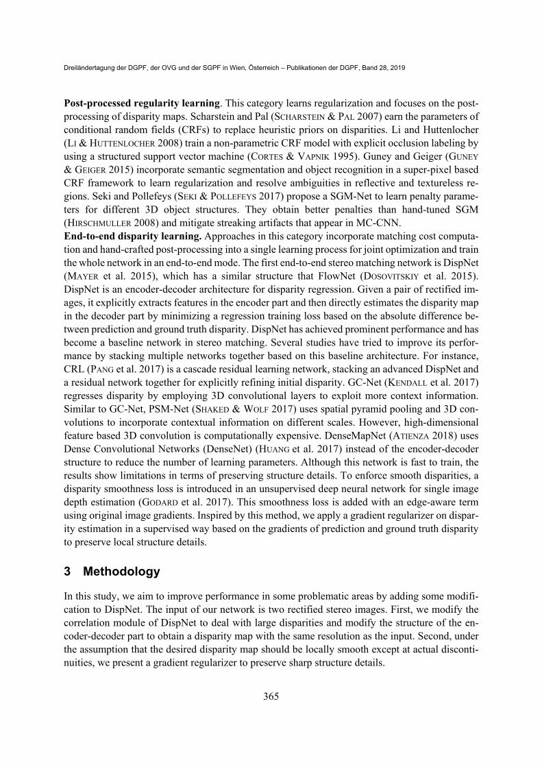
and channels, respectively. In order to obtain dense per-pixel predictions with the original input resolution, we apply 5 up-sampling blocks corresponding to six scales (1/32, 1/16,1/8, 1/4, 1/2, 𝑎𝑛𝑑 1 𝑜𝑓 𝑡ℎ𝑒 𝑖𝑛𝑝𝑢𝑡 𝑠𝑖𝑧𝑒) in the decoder part to refine the coarse representation. Each block consists of a 4×4 deconvolution layer with stride of 2 to up-sample the encoded output. Similar to DispNet, skip connections are also used in the decoder part to preserve both the high-level coarse and the low-level fine information. In addition, we connect the left original image with deconvolution features, as shown in Fig. 1, to output more accurate and full resolution dis-parity maps, which is different from DispNet.

Fig. 1: Architecture overview of proposed method

3.2 Complementary loss

We train our model end to end with supervised learning using ground truth disparity data. In order to preserve local structure details in the output disparity, we present a gradient regularizer as an auxiliary loss. So, the loss for training contains two parts: the disparity regression term and the gradient regression term. For the disparity regression loss ℒ , we use the end point error (EPE), the absolute Euclidean distance between the disparity D predicted by the model and the ground truth disparity 𝐷, averaged over the valid pixels. We adopt the ℓ norm to regularize prediction which is widely used in pre-vious methods. Thus, the disparity regression loss ℒ is formulated as:

ℒ ∑ 𝐷 , 𝐷 ,, ∈ (2)

where ‖∙‖ denotes the ℓ norm, 𝑣 represents all valid disparity pixels in 𝐷 and 𝑁 is the number of valid pixels. As ground truth disparity maps are sometimes sparse (e.g. KITTI dataset (GEIGER

et al. 2012; MENZE et al. 2015)), we average our loss over the valid pixels 𝑁 , for which ground truth labels are available. Besides the above disparity regression term, we use a new gradient term in our loss by considering large disparity discontinuities. We apply a new gradient regularizer on the disparity field to en-courage similar change of disparities in the predicted and the ground truth disparity map and thus achieve more effective regularization. This is a key difference between our method and DispNet. As depth discontinuities are often accompanied by large disparity gradients, horizontal and vertical gradients of the disparity map convey information about significant depth differences in the scene


368

and local structure, which can be used to improve the quality of disparity maps. We minimize differences between gradients of the estimated disparity map and the ground truth to achieve an increase in performance. We apply the ℓ norm to disparity gradients with the gradient regression loss ℒ defined as：

ℒ ∑ ∇ 𝐷 , ∇ 𝐷 , ∇ 𝐷 , ∇ 𝐷 ,, (3)

Where ‖∙‖ denotes the ℓ norm, ∇ and ∇ are the horizontal and vertical gradient of the disparity maps. This gradient regression term encourages an estimated disparity map to have a similar local structure as a target disparity map and also encourages the network to find a local optimum to balance between the disparity and the gradient structure of the surfaces. The network is trained by minimizing the loss function E which is a weighted sum of these two terms, while 𝜆 controls the relative importance of the gradient regularizer in the optimization.

𝐸 ℒ 𝜆 ℒ (4)

4 Experiments and Results

4.1 Dataset

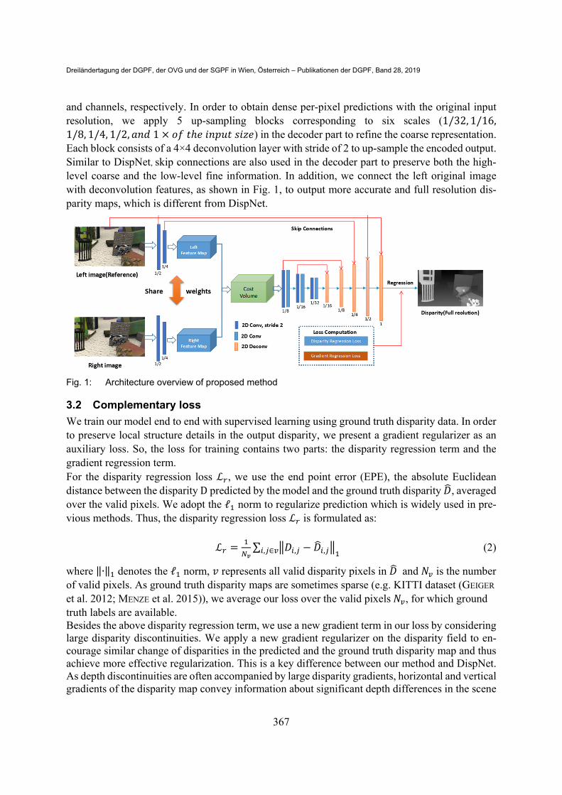
In this paper, we use the synthetic Scene Flow dataset to train our model, and then evaluate it on some public competitive synthetic and real stereo datasets. An overview of these datasets is given in Tab. 1.

Tab. 1 Overview of datasets used in our experiment

Dataset Name Frames for

training Frames

for testing Ground Dis-

parity Synthetic or Real World

Resolution

Scene Flow

FlyingThings3D 21818 4248 100%

Synthetic

960×540

Driving 8591 - 100% 960×540

Monkaa 4392 - 100% 960×540

KITTI dataset

KITTI2015 200 200 50%

(sparse) Real world

1242×375

KITTI2012 194 195 50%

(sparse) 1226×370

MPI Sintel 1064 564 100% Synthetic 1024×436

HCI 330 - Real world 656×541

Scene Flow (MAYER et al. 2015) is a large synthetic dataset for stereo matching, first designed and used in DispNet for training CNNs to estimate disparity. This dataset is rendered by computer graphics methods and provides accurate dense ground truth, which is large enough to train a com-plex network. It contains three subsets and has more than 39,000 stereo frames in 960×540 pixel resolution. In this paper, we only use the FlyingThings3D subset to train our model. The Driving and Monkaa datasets are only used to evaluate our method and baselines. The KITTI dataset was produced in 2012 (GEIGER et al. 2012) and extended in 2015 (MENZE et al. 2015, 2018). It contains stereo images of real-world complex road scenes collected from a cali-brated pair of cameras mounted on a driving car. It provides 200 stereo frames with sparse ground truth obtained from a 3D laser scanner. Since the laser only provides sparse data up to a certain


369

distance and height and labels in some areas (e.g. sky) are hard or impossible to obtain, the ground truth in these areas are not available. MPI Sintel (WULFF et al. 2012) is also an entirely synthetic dataset, which is created in the Blender software by rendering artificial scenes from a short open source animated 3D movie. It has 1064 training frames and provides dense ground truth disparities with large displacement, which is a very reliable test for comparison of methods. In this work, we use its final version because it con-tains sufficiently realistic scenes including natural image degradations. HCI (MEISTER et al. 2012) is a challenge outdoor dataset, which contains eleven real-world scenes with a huge variety of different weather conditions, different motion, and depth layers. It has 330 frames and no ground truth. In this work, we only use it to show the visual quality of our method.

4.2 Implementation details

Training: We implemented our architecture and training phase using the Tensorflow framework (ABADI et al. 2015) and optimized our model end-to-end by choosing the Adam optimizer with default momentum parameters, β1 = 0.9 and β2 = 0.999. Due to hardware limitations, we trained the network on a Titan X GPU with a mini batch size of 4 image pairs. The training images were resized to 368*760 and preprocessed by normalizing them to zero mean and a standard deviation of 1. Since we used ReLu as activation functions and observed that “He initialization” (HE et al. 2015) worked better for layers with ReLu activation, we chose the “He initialization” method to initialize the weights of our network. We set the starting learning rate λ to be 1e-4 and then divided it by half every 150k-th iteration after the first 200k iterations. To avoid overfittings, we employed L2 regularization with a weight decay strength d=0.0004. The training weights of our final model were obtained at the 719k-th iteration because there was no improvement for 5 consecutive vali-dations after this iteration. In addition, we performed online augmentation to introduce more var-iation in the training data, which includes geometric transformations (translation, scale) and chro-matic transformations (brightness, contrast, gamma, and color). Testing: we pre-trained our model on the FlyingThings3D dataset and evaluated it on other da-tasets. For evaluation of results, we used the EPE measure, which calculates the average Euclidean distance between predicted and ground truth disparity along all valid pixels. We also compared the performance of our method with other disparity estimation methods.

4.3 Results

In order to explore the effectiveness of our proposed method, we conduct two experiments on the aforementioned datasets. At the same time, we adopt DispNet as the baseline model; we present the qualitative and quantitative results. Tab. 2 reports the corresponding experiment results in terms of EPE, where “Baseline” represents the model of DispNet, “Model_Final” represents our final model with all modifications and “Model_NoG” is the model without gradient regularizer. By comparing the results of the “Model_Final” to the “Baseline”, we see that our model outperforms the baseline network in most cases and the EPE values are improved significantly (e.g. 27.9% on the Driving and 36.2% on the Sintel dataset). Since the Driving and Sintel datasets have larger disparities than the other datasets, the significant improvements on these two datasets can be directly attributed to our modification of the correlation module.


370

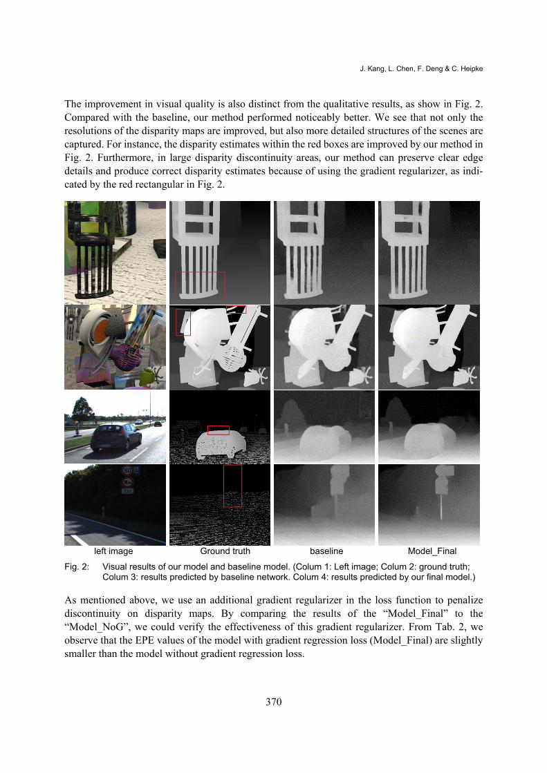
The improvement in visual quality is also distinct from the qualitative results, as show in Fig. 2. Compared with the baseline, our method performed noticeably better. We see that not only the resolutions of the disparity maps are improved, but also more detailed structures of the scenes are captured. For instance, the disparity estimates within the red boxes are improved by our method in Fig. 2. Furthermore, in large disparity discontinuity areas, our method can preserve clear edge details and produce correct disparity estimates because of using the gradient regularizer, as indi-cated by the red rectangular in Fig. 2.

left image Ground truth baseline Model_Final

Fig. 2: Visual results of our model and baseline model. (Colum 1: Left image; Colum 2: ground truth; Colum 3: results predicted by baseline network. Colum 4: results predicted by our final model.)

As mentioned above, we use an additional gradient regularizer in the loss function to penalize discontinuity on disparity maps. By comparing the results of the “Model_Final” to the “Model_NoG”, we could verify the effectiveness of this gradient regularizer. From Tab. 2, we observe that the EPE values of the model with gradient regression loss (Model_Final) are slightly smaller than the model without gradient regression loss.


371

Tab. 2: EPE of different models on different datasets. The last row shows the improved accuracy when comparing ‘Model_Final’ to the baseline (first number) and to ‘Model_NoG’ (second number)

Dataset Flying3D Monkaa Driving Sintel KITTI2015 KITTI2012

Baseline 1.68 5.78 12.46 5.66 1.59 1.55

Model_NoG 1.74 4.60 9.53 3.66 1.56 1.49

Model_Final 1.71 4.58 8.98 3.61 1.54 1.43

Improved(%) -1.8/1.2 20.8/0.4 27.9/5.8 36.2/1.4 3.1/1.3 7.7/4.0

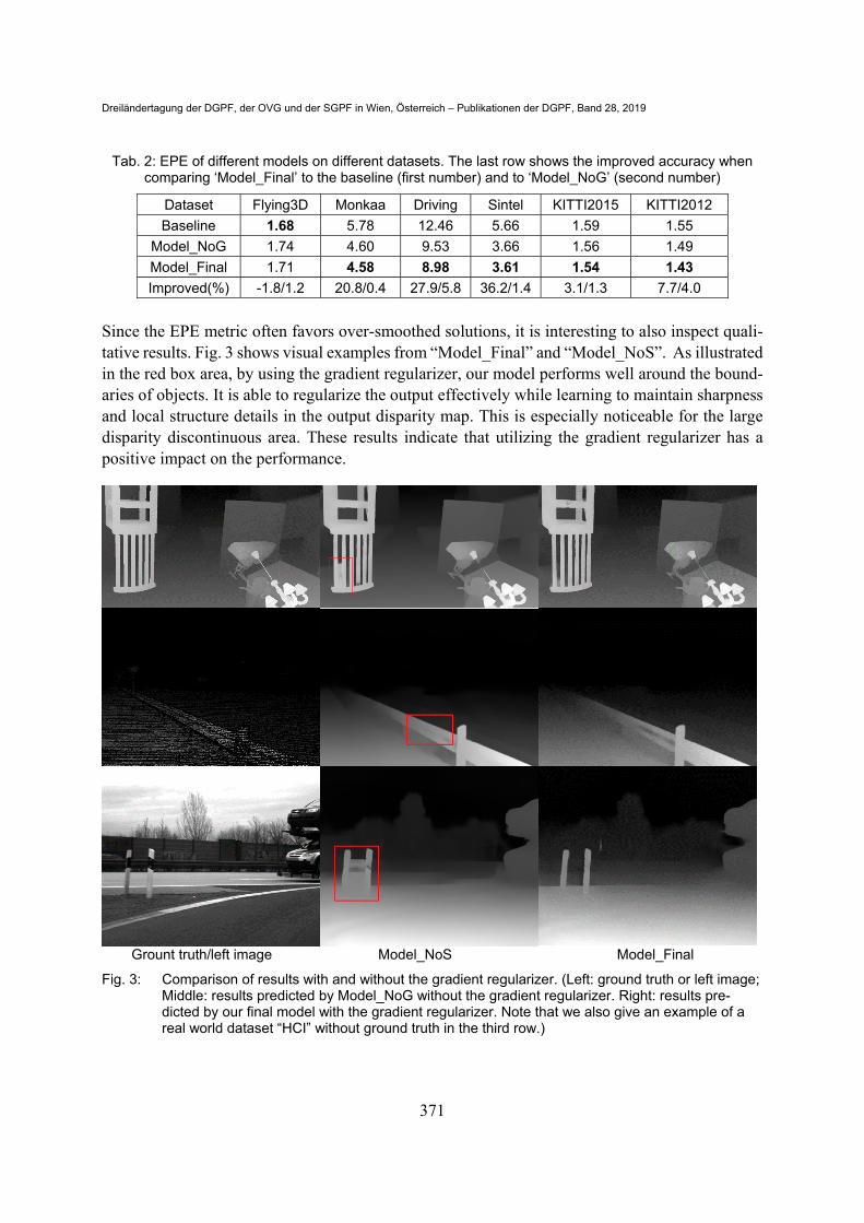
Since the EPE metric often favors over-smoothed solutions, it is interesting to also inspect quali-tative results. Fig. 3 shows visual examples from “Model_Final” and “Model_NoS”. As illustrated in the red box area, by using the gradient regularizer, our model performs well around the bound-aries of objects. It is able to regularize the output effectively while learning to maintain sharpness and local structure details in the output disparity map. This is especially noticeable for the large disparity discontinuous area. These results indicate that utilizing the gradient regularizer has a positive impact on the performance.

Grount truth/left image Model_NoS Model_Final

Fig. 3: Comparison of results with and without the gradient regularizer. (Left: ground truth or left image; Middle: results predicted by Model_NoG without the gradient regularizer. Right: results pre-dicted by our final model with the gradient regularizer. Note that we also give an example of a real world dataset “HCI” without ground truth in the third row.)


372

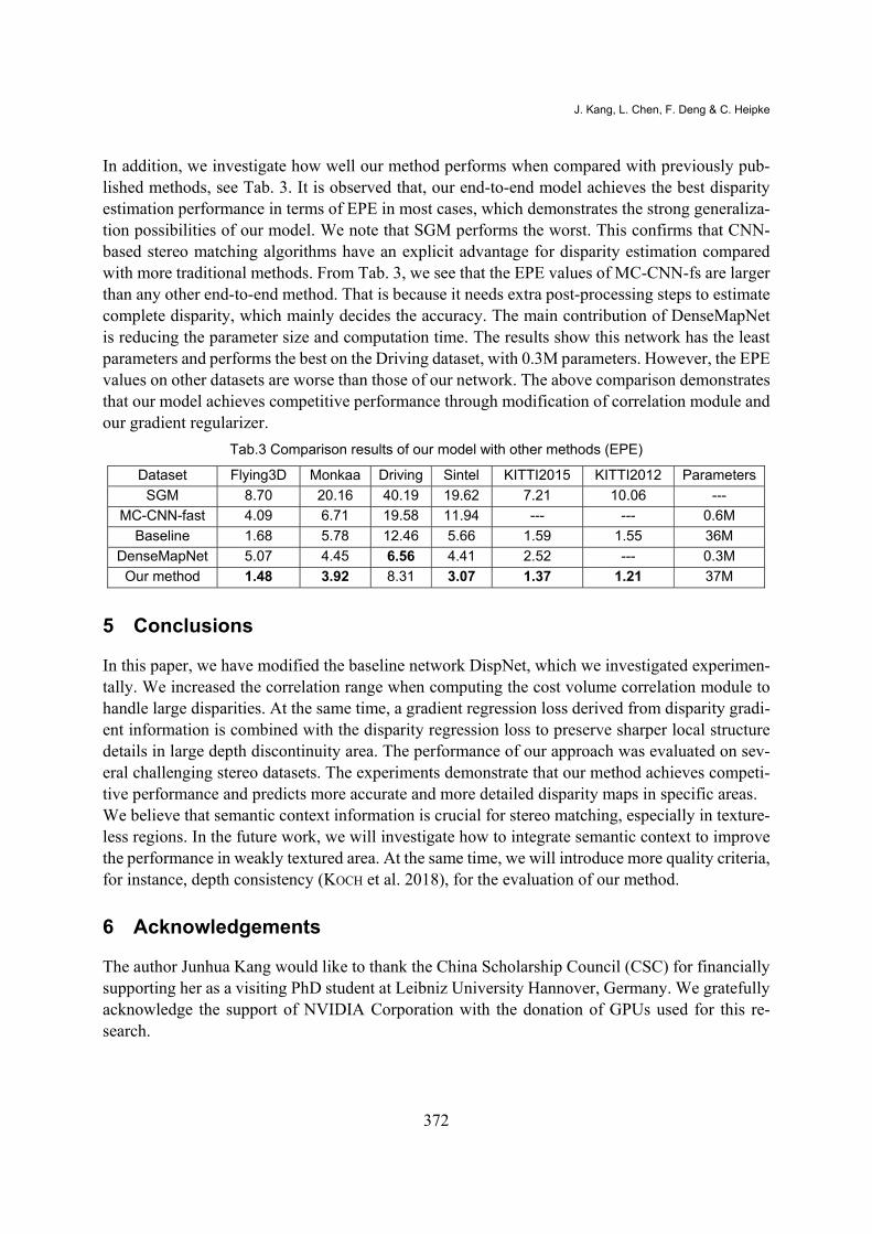
In addition, we investigate how well our method performs when compared with previously pub-lished methods, see Tab. 3. It is observed that, our end-to-end model achieves the best disparity estimation performance in terms of EPE in most cases, which demonstrates the strong generaliza-tion possibilities of our model. We note that SGM performs the worst. This confirms that CNN-based stereo matching algorithms have an explicit advantage for disparity estimation compared with more traditional methods. From Tab. 3, we see that the EPE values of MC-CNN-fs are larger than any other end-to-end method. That is because it needs extra post-processing steps to estimate complete disparity, which mainly decides the accuracy. The main contribution of DenseMapNet is reducing the parameter size and computation time. The results show this network has the least parameters and performs the best on the Driving dataset, with 0.3M parameters. However, the EPE values on other datasets are worse than those of our network. The above comparison demonstrates that our model achieves competitive performance through modification of correlation module and our gradient regularizer.

Tab.3 Comparison results of our model with other methods (EPE)

Dataset Flying3D Monkaa Driving Sintel KITTI2015 KITTI2012 Parameters

SGM 8.70 20.16 40.19 19.62 7.21 10.06 ---

MC-CNN-fast 4.09 6.71 19.58 11.94 --- --- 0.6M

Baseline 1.68 5.78 12.46 5.66 1.59 1.55 36M

DenseMapNet 5.07 4.45 6.56 4.41 2.52 --- 0.3M

Our method 1.48 3.92 8.31 3.07 1.37 1.21 37M

5 Conclusions

In this paper, we have modified the baseline network DispNet, which we investigated experimen-tally. We increased the correlation range when computing the cost volume correlation module to handle large disparities. At the same time, a gradient regression loss derived from disparity gradi-ent information is combined with the disparity regression loss to preserve sharper local structure details in large depth discontinuity area. The performance of our approach was evaluated on sev-eral challenging stereo datasets. The experiments demonstrate that our method achieves competi-tive performance and predicts more accurate and more detailed disparity maps in specific areas. We believe that semantic context information is crucial for stereo matching, especially in texture-less regions. In the future work, we will investigate how to integrate semantic context to improve the performance in weakly textured area. At the same time, we will introduce more quality criteria, for instance, depth consistency (KOCH et al. 2018), for the evaluation of our method.

6 Acknowledgements

The author Junhua Kang would like to thank the China Scholarship Council (CSC) for financially supporting her as a visiting PhD student at Leibniz University Hannover, Germany. We gratefully acknowledge the support of NVIDIA Corporation with the donation of GPUs used for this re-search.


373

7 References

ABADI, M., AGARWAL, A., BARHAM, P., BREVDO, E., CHEN, Z., CITRO, C., CORRADO, G., DAVIS, A., DEAN, J. & DEVIN, M., 2015: Tensorflow: Large-scale machine learning on heterogeneous distributed systems.

ATIENZA, R., 2018: Fast Disparity Estimation using Dense Networks. arXiv preprint arXiv:1805.07499.

CHEN, J. & YUAN, C., 2016: Convolutional neural network using multi-scale information for stereo matching cost computation. IEEE International Conference on Image Processing, 3424-3428.

CORTES, C. & VAPNIK, V., 1995: Support-vector networks. Machine Learning, 20, 273–297.

DOSOVITSKIY, A., FISCHERY, P., ILG, E., HAUSSER, P., HAZIRBAS, C., GOLKOV, V., SMAGT, P. VAN

DER, CREMERS, D. & BROX, T., 2015: FlowNet: Learning optical flow with convolutional networks. IEEE International Conference on Computer Vision, 2758-2766.

GEIGER, A., LENZ, P. & URTASUN, R., 2012: Are we ready for autonomous driving? the kitti vision benchmark suite. IEEE Conference on Computer Vision and Pattern Recognition, 3354-3361.

GODARD, C., MAC AODHA, O. & BROSTOW, G. J., 2017: Unsupervised monocular depth estimation with left-right consistency. CVPR., Vol. 2p. 7.

GUNEY, F. & GEIGER, A., 2015: Displets: Resolving stereo ambiguities using object knowledge. IEEE Conference on Computer Vision and Pattern Recognition, 4165-4175.

HE, K., ZHANG, X., REN, S. & SUN, J., 2015: Delving deep into rectifiers: Surpassing human-level performance on imagenet classification. IEEE International Conference on Computer Vision, 1026-1034.

HIRSCHMULLER, H., 2008: Stereo processing by semiglobal matching and mutual information. IEEE Transactions on pattern analysis and machine intelligence, 30, 328-341.

HUANG, G., LIU, Z., VAN DER MAATEN, L. & WEINBERGER, K. Q., 2017: Densely connected convolutional networks. CVPR., Vol. 1p. 3.

KENDALL, A., MARTIROSYAN, H., DASGUPTA, S., HENRY, P., KENNEDY, R., BACHRACH, A. & BRY, A., 2017: End-to-End Learning of Geometry and Context for Deep Stereo Regression. IEEE International Conference on Computer Vision, 66-75.

KOCH, T., LIEBEL, L., FRAUNDORFER, F. & KÖRNER, M., 2018: Evaluation of CNN-based single-image depth estimation methods. arXiv preprint arXiv:1805.01328.

LECUN, Y., BOTTOU, L., BENGIO, Y. & HAFFNER, P., 1998: Gradient-based learning applied to document recognition. Proceedings of the IEEE., 86, 2278-2324.

LI, Y. & HUTTENLOCHER, D. P., 2008: Learning for stereo vision using the structured support vector machine. IEEE Conference on Computer Vision and Pattern Recognition, 1-8.

LUO, W., SCHWING, A. G. & URTASUN, R., 2016: Efficient deep learning for stereo matching. IEEE Conference on Computer Vision and Pattern Recognition, 5695-5703.

MAYER, N., ILG, E., HÄUSSER, P., FISCHER, P., CREMERS, D., DOSOVITSKIY, A. & BROX, T., 2015: A Large Dataset to Train Convolutional Networks for Disparity, Optical Flow, and Scene Flow Estimation. IEEE Conference on Computer Vision and Pattern Recognition, 4040-4048.


374

MEISTER, S., JÄHNE, B. & KONDERMANN, D., 2012: Outdoor stereo camera system for the generation of real-world benchmark data sets. Optical Engineering, 51, 21107.

MENZE, M., HEIPKE, C. & GEIGER, A., 2015: Joint 3d estimation of vehicles and scene flow. ISPRS Workshop on Image Sequence Analysis (ISA), 8.

MENZE, M., HEIPKE, C. & GEIGER, A., 2018: Object scene flow. ISPRS Journal of Photogrammetry and Remote Sensing, 140, 60-76.

PANG, J., SUN, W., REN, J. S. J., YANG, C. & YAN, Q., 2017: Cascade Residual Learning: A Two-Stage Convolutional Neural Network for Stereo Matching. ICCV Workshops, 7.

SCHARSTEIN, D. & SZELISKI, R., 2002: A taxonomy and evaluation of dense two-frame stereo correspondence algorithms. International Journal of Computer Vision, 47, 7-42.

SCHARSTEIN, D. & PAL, C., 2007: Learning conditional random fields for stereo. IEEE Conference on Computer Vision and Pattern Recognition, 1-8.

SEKI, A. & POLLEFEYS, M., 2017: SGM-Nets: Semi-global matching with neural networks. Proceedings of the 2017 IEEE Conference on Computer Vision and Pattern Recognition, 21-26.

SHAKED, A. & WOLF, L., 2017: Improved stereo matching with constant highway networks and reflective confidence learning. IEEE Conference on Computer Vision and Pattern Recognition, 6901-6910.

WULFF, J., BUTLER, D. J., STANLEY, G. B. & BLACK, M. J., 2012: Lessons and insights from creating a synthetic optical flow benchmark. European Conference on Computer Vision. Springer, 168-177.

ZBONTAR, J. & LECUN, Y., 2016: Stereo matching by training a convolutional neural network to compare image patches. Journal of Machine Learning Research., 17, 2.

Documents

Encoder-Decoder network for local structure preserving ... · DispNet is an encoder-decoder architecture for disparity regression. Given a pair of rectified im-ages, it explicitly