The Cryosphere, 8, 439–451, 2014www.the-cryosphere.net/8/439/2014/doi:10.5194/tc-8-439-2014© Author(s) 2014. CC Attribution 3.0 License.

The Cryosphere

Open A

ccess

Empirical sea ice thickness retrieval during the freeze-up periodfrom SMOS high incident angle observations

M. Huntemann1, G. Heygster1, L. Kaleschke2, T. Krumpen3, M. Mäkynen4, and M. Drusch5

1Institute of Environmental Physics, University of Bremen, Bremen, Germany2Institute of Oceanography, University of Hamburg, Hamburg, Germany3Alfred Wegener Institute, Bremerhaven, Germany4Finnish Meteorological Institute, Helsinki, Finland5ESTEC, ESA, Noordwijk, Netherlands

Correspondence to:M. Huntemann (marcus.huntemann@uni-bremen.de)

Received: 30 July 2013 – Published in The Cryosphere Discuss.: 30 August 2013Revised: 20 January 2014 – Accepted: 10 February 2014 – Published: 18 March 2014

Abstract. Sea ice thickness information is important for seaice modelling and ship operations. Here a method to detectthe thickness of sea ice up to 50 cm during the freeze-up sea-son based on high incidence angle observations of the SoilMoisture and Ocean Salinity (SMOS) satellite working at1.4 GHz is suggested. By comparison of thermodynamic icegrowth data with SMOS brightness temperatures, a high cor-relation to intensity and an anticorrelation to the differencebetween vertically and horizontally polarised brightness tem-peratures at incidence angles between 40 and 50◦ are foundand used to develop an empirical retrieval algorithm sensitiveto thin sea ice up to 50 cm thickness. The algorithm showshigh correlation with ice thickness data from airborne mea-surements and reasonable ice thickness patterns for the Arc-tic freeze-up period.

1 Introduction

Sea ice is an essential climate component and observationsof its formation, evolution, and decay are important for un-derstanding and predicting climate change. Sea ice cover-age has been observed since 1972 using several microwaveradiometers, namely the Electrically Scanning MicrowaveRadiometer (ESMR) (1972–1977), Scanning Multi-channelMicrowave Radiometer (SMMR) (1978–1987), Special Sen-sor Microwave Imager (SSM/I) (1987–present), AdvancedMicrowave Scanning Radiometer – Earth Observing System(EOS) (AMSRE) (2002–2012) and AMSR2 (2012–present).

The sensitivity of the microwave emission of sea ice has beennarrowed down to a few essential microphysical propertieslike sea ice thickness, salinity, temperature and snow grainsize (Tonboe et al., 2011; Fuhrhop et al., 1998). Since 2009the ESA (European Space Agency) Soil Moisture and OceanSalinity (SMOS) mission, has been observing the Earth at1.4 GHz (L-band), from a sun synchronous dusk–dawn orbit(Kerr et al., 2001). At this microwave frequency, the pene-tration depth into sea ice is about 50 cm and even more intoice of less saline waters like the Baltic Sea (Kaleschke et al.,2010).

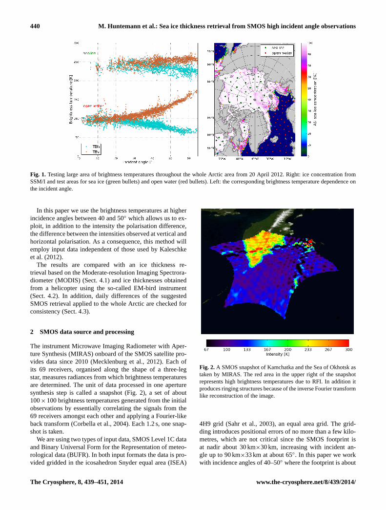
Figure1 (left) illustrates the basic situation: the brightnesstemperature of open water at nadir is around 100 K. For verti-cal polarisation, it increases with incidence angle up to 180 Kat 65◦, and for horizontal polarisation it decreases down toabout 60 K. At all incidence angles, the signal of sea ice isclearly higher. The vertically polarised emission increasesfrom 230 K at nadir to 260 K at 65◦, and the horizontally po-larised emission decreasing down to 215 K.

Because of the high penetration depth at L band and thehigh brightness temperature contrast of over 100 K betweenice and open water, increasing sea ice thickness is reflectedin the L-band emission. Therefore it appears attractive to as-sess the potential of retrieving sea ice thickness (SIT) withSMOS. Kaleschke et al.(2010, 2012) first showed that forobservations of up to 40◦ incident angle, the intensity can beused to obtain information on the sea ice thickness.

Published by Copernicus Publications on behalf of the European Geosciences Union.

440 M. Huntemann et al.: Sea ice thickness retrieval from SMOS high incident angle observationsD

iscussionPaper

|D

iscussionPaper

|D

iscussionPaper

|D

iscussionPaper

|

Fig. 1. Testing large area of brightness temperatures throughout the whole Arctic area from 20 April2012. Right: ice concentration from SSMIS and test areas for sea ice (green bullets) and open water (redbullets). Left: the corresponding brightness temperature dependence on the incident angle.

22

Fig. 1. Testing large area of brightness temperatures throughout the whole Arctic area from 20 April 2012. Right: ice concentration fromSSM/I and test areas for sea ice (green bullets) and open water (red bullets). Left: the corresponding brightness temperature dependence onthe incident angle.

In this paper we use the brightness temperatures at higherincidence angles between 40 and 50◦ which allows us to ex-ploit, in addition to the intensity the polarisation difference,the difference between the intensities observed at vertical andhorizontal polarisation. As a consequence, this method willemploy input data independent of those used byKaleschkeet al.(2012).

The results are compared with an ice thickness re-trieval based on the Moderate-resolution Imaging Spectrora-diometer (MODIS) (Sect.4.1) and ice thicknesses obtainedfrom a helicopter using the so-called EM-bird instrument(Sect.4.2). In addition, daily differences of the suggestedSMOS retrieval applied to the whole Arctic are checked forconsistency (Sect.4.3).

2 SMOS data source and processing

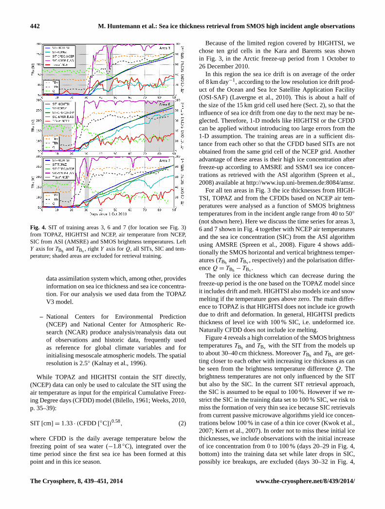
The instrument Microwave Imaging Radiometer with Aper-ture Synthesis (MIRAS) onboard of the SMOS satellite pro-vides data since 2010 (Mecklenburg et al., 2012). Each ofits 69 receivers, organised along the shape of a three-legstar, measures radiances from which brightness temperaturesare determined. The unit of data processed in one aperturesynthesis step is called a snapshot (Fig.2), a set of about100×100 brightness temperatures generated from the initialobservations by essentially correlating the signals from the69 receivers amongst each other and applying a Fourier-likeback transform (Corbella et al., 2004). Each 1.2 s, one snap-shot is taken.

We are using two types of input data, SMOS Level 1C dataand Binary Universal Form for the Representation of meteo-rological data (BUFR). In both input formats the data is pro-vided gridded in the icosahedron Snyder equal area (ISEA)

Fig. 2.A SMOS snapshot of Kamchatka and the Sea of Okhotsk astaken by MIRAS. The red area in the upper right of the snapshotrepresents high brightness temperatures due to RFI. In addition itproduces ringing structures because of the inverse Fourier transformlike reconstruction of the image.

4H9 grid (Sahr et al., 2003), an equal area grid. The grid-ding introduces positional errors of no more than a few kilo-metres, which are not critical since the SMOS footprint isat nadir about 30 km×30 km, increasing with incident an-gle up to 90 km×33 km at about 65◦. In this paper we workwith incidence angles of 40–50◦ where the footprint is about

The Cryosphere, 8, 439–451, 2014 www.the-cryosphere.net/8/439/2014/

M. Huntemann et al.: Sea ice thickness retrieval from SMOS high incident angle observations 441

Fig. 3.Location of training areas.

50 km×31 km. As each footprint overlaps several grid points(Castro, 2008), the data of neighbouring grid points are cor-related.

The L1C data cover the whole ISEA 4H9 discrete globalgrid (DGG), but are available with an about 24–48 h delay.As for operational sea ice services, a shorter delay is re-quired, the BUFR data, offering SMOS data with only a 3–4 h delay, are used. In order to reduce the data volume, overthe ocean in the BUFR data only every other DGG cell isrepresented.

Even though the frequency band near 1.4 GHz is not al-lowed for communication, RFIs (radio frequency interfer-ences) have been strong during the early phase of the SMOSmission. They have been reduced since then, but not com-pletely eliminated (Camps et al., 2010; Oliva et al., 2012).

The RFI-influenced data shows mostly higher brightnesstemperatures (Tb) than occur in nature. All surface emissionsof more thanTb = 300 K are unrealistic because they wouldrequire an emissivity larger than unity and are taken as RFI inour processing. Due to the Fourier-transform-like reconstruc-tion of the snapshots, a strong RFI from a single source onEarth’s surface may extend over the whole snapshot, albeit atlower values. In order to also discard lower RFI influences,in our processing the whole snapshot is discarded if at leastone pixel shows a brightness temperature larger than 300 K.An example of RFI can be seen in the snapshot in Fig.2.

Since May 2010, SMOS has been operating in full po-larisation mode, i.e. measuring all four Stokes components.However, these are delivered in the L1C and BUFR data setswith respect to the instrument reference plane (X, Y ) andneed to be converted to Earth’s surface plane (V , H ) by thetransformation

A1A2A3A4

=

cos2(α) sin2(α) −cos(α)sin(α) 0sin2(α) cos2(α) cos(α)sin(α) 0sin(2α) −sin(2α) cos(2α) 0

0 0 0 1

T BH

T BV

T B3T B4

,

(1)

with A1 = <(T BXX),A2 = <(T BYY ),A3 =

2=(T BXY ),A4 = −2=(T BXY ) andα = αr +ωFα , whereαr

andωFα are geometric rotation angle and Faraday rotationangle, respectively (Zine et al., 2008), which are supplied inthe SMOS L1C and BUFR data.<(...) and=(...) are the realand imaginary parts, respectively.

The transformation needs for each observation in the (V ,H ) frame brightness temperatures at three polarisations:XX,YY andXY . However, only one (eitherXX or YY ) or twoof them (either (XX, XY ) or (YY , XY )) are measured withinone snapshot so that either one or two missing values need tobe interpolated.

We use observations from neighbouring, overlappingsnapshots acquired within 2.5 s before or after the time ofinterest (SMOS takes snapshots every 1.2 s). Within 2.5 s theatmosphere and surface conditions should change only lit-tle. If no suitable values for interpolation can be found, thisobservation is discarded from the transformation and furtherdata analysis. As an additional condition, the incidence anglemay only vary less than 0.5◦, which ensures the accuracy ofthe interpolation since the polarised brightness temperaturesvary quite strongly at 40–50◦ incident angles (Fig.1).

3 Sea ice thickness retrieval method

The first step to develop a fully empirical retrieval was to gettraining data and analyse it for consistency. Since SIT of thinice during the freeze-up period is hard to observe in situ (onecannot stand or walk on it), we had to rely on other, modelbased sources as a reference for comparison.

– The HIGHTSI (Launiainen and Cheng, 1998), aregional, thermodynamic one-dimensional sea icegrowth model driven by the High Resolution LimitedArea Model (HIRLAM), (Källen, 1996; Unden et al.,2002), a short-range weather forecasting system in-tended to use for limited areas developed by elevenEuropean countries (www.hirlam.org). HIGHTSI wasemployed to model the freeze-up period 2010 in theBarents Sea and Kara Sea.

– Towards an Operational Prediction system for theNorth Atlantic European coastal Zones (TOPAZ)(Sakov et al., 2012), a coupled global ocean–sea ice

www.the-cryosphere.net/8/439/2014/ The Cryosphere, 8, 439–451, 2014

442 M. Huntemann et al.: Sea ice thickness retrieval from SMOS high incident angle observations

Fig. 4. SIT of training areas 3, 6 and 7 (for location see Fig.3)from TOPAZ, HIGHTSI and NCEP, air temperature from NCEP,SIC from ASI (AMSRE) and SMOS brightness temperatures. LeftY axis forTBh andTBv , right Y axis forQ, all SITs, SIC and tem-perature; shaded areas are excluded for retrieval training.

data assimilation system which, among other, providesinformation on sea ice thickness and sea ice concentra-tion. For our analysis we used data from the TOPAZV3 model.

– National Centers for Environmental Prediction(NCEP) and National Center for Atmospheric Re-search (NCAR) produce analysis/reanalysis data outof observations and historic data, frequently usedas reference for global climate variables and forinitialising mesoscale atmospheric models. The spatialresolution is 2.5◦ (Kalnay et al., 1996).

While TOPAZ and HIGHTSI contain the SIT directly,(NCEP) data can only be used to calculate the SIT using theair temperature as input for the empirical Cumulative Freez-ing Degree days (CFDD) model (Bilello, 1961; Weeks, 2010,p. 35–39):

SIT [cm] = 1.33· (CFDD [◦C])0.58, (2)

where CFDD is the daily average temperature below thefreezing point of sea water (−1.8◦C), integrated over thetime period since the first sea ice has been formed at thispoint and in this ice season.

Because of the limited region covered by HIGHTSI, wechose ten grid cells in the Kara and Barents seas shownin Fig. 3, in the Arctic freeze-up period from 1 October to26 December 2010.

In this region the sea ice drift is on average of the orderof 8 km day−1, according to the low resolution ice drift prod-uct of the Ocean and Sea Ice Satellite Application Facility(OSI-SAF) (Lavergne et al., 2010). This is about a half ofthe size of the 15 km grid cell used here (Sect.2), so that theinfluence of sea ice drift from one day to the next may be ne-glected. Therefore, 1-D models like HIGHTSI or the CFDDcan be applied without introducing too large errors from the1-D assumption. The training areas are in a sufficient dis-tance from each other so that the CFDD based SITs are notobtained from the same grid cell of the NCEP grid. Anotheradvantage of these areas is their high ice concentration afterfreeze-up according to AMSRE and SSM/I sea ice concen-trations as retrieved with the ASI algorithm (Spreen et al.,2008) available athttp://www.iup.uni-bremen.de:8084/amsr.

For all ten areas in Fig.3 the ice thicknesses from HIGH-TSI, TOPAZ and from the CFDDs based on NCEP air tem-peratures were analysed as a function of SMOS brightnesstemperatures from in the incident angle range from 40 to 50◦

(not shown here). Here we discuss the time series for areas 3,6 and 7 shown in Fig.4 together with NCEP air temperaturesand the sea ice concentration (SIC) from the ASI algorithmusing AMSRE (Spreen et al., 2008). Figure4 shows addi-tionally the SMOS horizontal and vertical brightness temper-atures (TBh andTBv , respectively) and the polarisation differ-enceQ = TBh − TBv .

The only ice thickness which can decrease during thefreeze-up period is the one based on the TOPAZ model sinceit includes drift and melt. HIGHTSI also models ice and snowmelting if the temperature goes above zero. The main differ-ence to TOPAZ is that HIGHTSI does not include ice growthdue to drift and deformation. In general, HIGHTSI predictsthickness of level ice with 100 % SIC, i.e. undeformed ice.Naturally CFDD does not include ice melting.

Figure4 reveals a high correlation of the SMOS brightnesstemperaturesTBh andTBv with the SIT from the models upto about 30–40 cm thickness. MoreoverTBh andTBv are get-ting closer to each other with increasing ice thickness as canbe seen from the brightness temperature differenceQ. Thebrightness temperatures are not only influenced by the SITbut also by the SIC. In the current SIT retrieval approach,the SIC is assumed to be equal to 100 %. However if we re-strict the SIC in the training data set to 100 % SIC, we risk tomiss the formation of very thin sea ice because SIC retrievalsfrom current passive microwave algorithms yield ice concen-trations below 100 % in case of a thin ice cover (Kwok et al.,2007; Kern et al., 2007). In order not to miss these initial icethicknesses, we include observations with the initial increaseof ice concentration from 0 to 100 % (days 20–29 in Fig.4,bottom) into the training data set while later drops in SIC,possibly ice breakups, are excluded (days 30–32 in Fig.4,

The Cryosphere, 8, 439–451, 2014 www.the-cryosphere.net/8/439/2014/

M. Huntemann et al.: Sea ice thickness retrieval from SMOS high incident angle observations 443

Fig. 5. Dependence of polarisation difference (top) and inten-sity (bottom) to ice thicknesses obtained from CFDD fromNCEP/NCAR surface air temperature data. Red line shows a fit ofan empirical function of polarisation difference and intensity to icethickness.

bottom). Excluded areas are shaded grey in Fig.4. Similar in-vestigations have been carried out for all 10 regions in Fig.3(Heygster et al., 2012).

In several of the regions, SIT did not increase monotoni-cally as SIC decreased over longer periods or freeze-up waslate in the investigation period. As a result, only areas 3, 6and 7 show monotonic freeze-up periods sufficiently con-tiguous for our analysis (Fig.4). As ice forms there is ahigh correlation of temperature to the brightness tempera-tures measured by SMOS. Since the temperature drives theCFDD based ice thickness model this correlation is expected.However, the air temperature does not seem to have a directinfluence on the brightness temperature in case of thicker ice.In area 3 (day 67), area 6 (day 37) and area 7 (days 60 and73) an increase in temperature is connected with a drop ofSIC to about 90 %. Overall the temperatures are relativelystable around−20◦C without any melt events in these threeregions. TOPAZ shows considerably lower SIT in area 3 thanthe other non-dynamic models. However, we tend to trust theHIGHTSI and NCEP based thicknesses as the temperature isalmost all the time below−20◦C where a steady ice thick-ness growth is expected. Between theI andQ parametersand SIT obtained from the models for each of the differenttraining areas the following functions are fitted:

Iabc(x) = a − (a − b) · exp(−x/c), (3)

Qabcd(x) = (a − b) · exp(−(x/c)d) + b . (4)

Equation (3) is also used inKaleschke et al.(2012) andis basically the Lambert–Beer law. Equation (4) was chosenempirically since it allows us to represent the shape of thick-ness dependence of the polarisation difference in an appro-priate way.

Fig. 6. Retrieval curve of SIT fromI andQ. Dot colours belongto different regions (see Fig.3). Numbers at the curve mark theretrieved SIT in centimetre. Observation point P can be synthesisedby observing thicknesses of 0 and 40 cm (blue line) in one footprint.

Table 1.Parameters for fit function in Eqs. (3) and (4).

Parameter a [K] b [K] c [cm] d

Iabc 234.1 100.2 12.7 –Qabcd 44.8 19.4 24.1 2.1

Figure5 shows the relation between the SIT and the po-larisation differenceQ and intensityI , respectively, in ourtraining data set. The sensitivity ofI to sea ice thickness de-creases from 30 cm onwards, whereasQ is sensitive up toabout 50 cm, considering their range of variation. However,it is important to mention here that the relative error of thebrightness temperature difference is higher than it is with theintensity.

For training, only the CFDD derived SIT from NCEP datais used, so that the HIRLAM based MODIS retrieval mayserve in the next section as independent comparison data.Since HIGHTSI is also driven by HIRLAM, HIGHTSI datais not used for training. Table1 shows the optimal parametersfor Eq. (3) which best represent the training data set as seenin Fig. 5.

Figure6 shows the two functions as a parameterised curvein the (Q, I ) plane. The colour of the points indicates thedifferent regions (Fig.3). The curved black line representsthe SIT retrieved for a given pair (Q, I ). To find the SITfor given I andQ, the minimum Euclidean distance to theretrieval curve is determined. Figure6 shows that changes inQ only influence the retrieved SIT at higher intensities, i.e.SIT higher than 30 cm as expected from Fig.5.

At higher SIT the returned values are sensitive even tosmall changes of the observedI and Q. The uncertaintyof the instrument is about 2–3 K for a single measurement(Brown et al., 2008). The error budget of daily averageswithin one grid cell is reduced by the averaging over the

www.the-cryosphere.net/8/439/2014/ The Cryosphere, 8, 439–451, 2014

444 M. Huntemann et al.: Sea ice thickness retrieval from SMOS high incident angle observations

Fig. 7. Comparison between SMOS (top left) and MODIS (top centre) retrieved SIT for 4 December 2010 in the Kara Sea. The validMODIS data after averaging to the SMOS footprint size (top right). The scatter plot of MODIS and SMOS for all MODIS data from24 November 2010 to 14 April 2011 (71 scenes) (bottom). Regression line (red):y = 1.75x −5.73, RMSD= 11 cm, correlation ofr = 0.68.

incidence angle range of 40–50◦, but increased by the emis-sivity variations with incidence angle (Fig.1, left). As thesensitivity of the retrieved SIT to both intensity and polari-sation difference increases strongly with SIT (Figs.5, 6), theretrieval is cut off at 50 cm SIT.

Higher retrieved values are marked by a flag for more than50 cm but no distinct values are returned.

It should be mentioned that the retrieval in the presentform assumes ice concentrations of 100 %. Introducing asecond observationQ in the retrieval would in principle al-low us to determine simultaneously a second parameter, e.g.the ice concentration. An example observation,P = (Q, I )(Fig. 6), could then be explained as a linear combination ofopen water (ice thickness 0 cm) and 40 cm thick ice. How-ever, attempts to establish such a two-parameter retrieval

have turned out to be quite noisy (Heygster et al., 2012).Therefore, here we refrain from a two-parameter retrieval.The advantage of introducing a second parameter is rather again of sensitivity in the upper range of ice thicknesses.

3.1 Error estimation

For each 10 cm interval of the training NCEP CFDD SIT,the RMSD (root mean square deviation) to the SIT retrievedfrom SMOS is shown in Table2. The uncertainty is about30 % of the retrieved value. The retrieval of very thin ice of0–20 cm is quite accurate and stable. Higher retrieved SITshave a larger uncertainty and because of the restriction ofthe SIT retrieval to 50 cm, it might yield larger than stateddeviations close to the 50 cm border. The RMSD values in

The Cryosphere, 8, 439–451, 2014 www.the-cryosphere.net/8/439/2014/

M. Huntemann et al.: Sea ice thickness retrieval from SMOS high incident angle observations 445

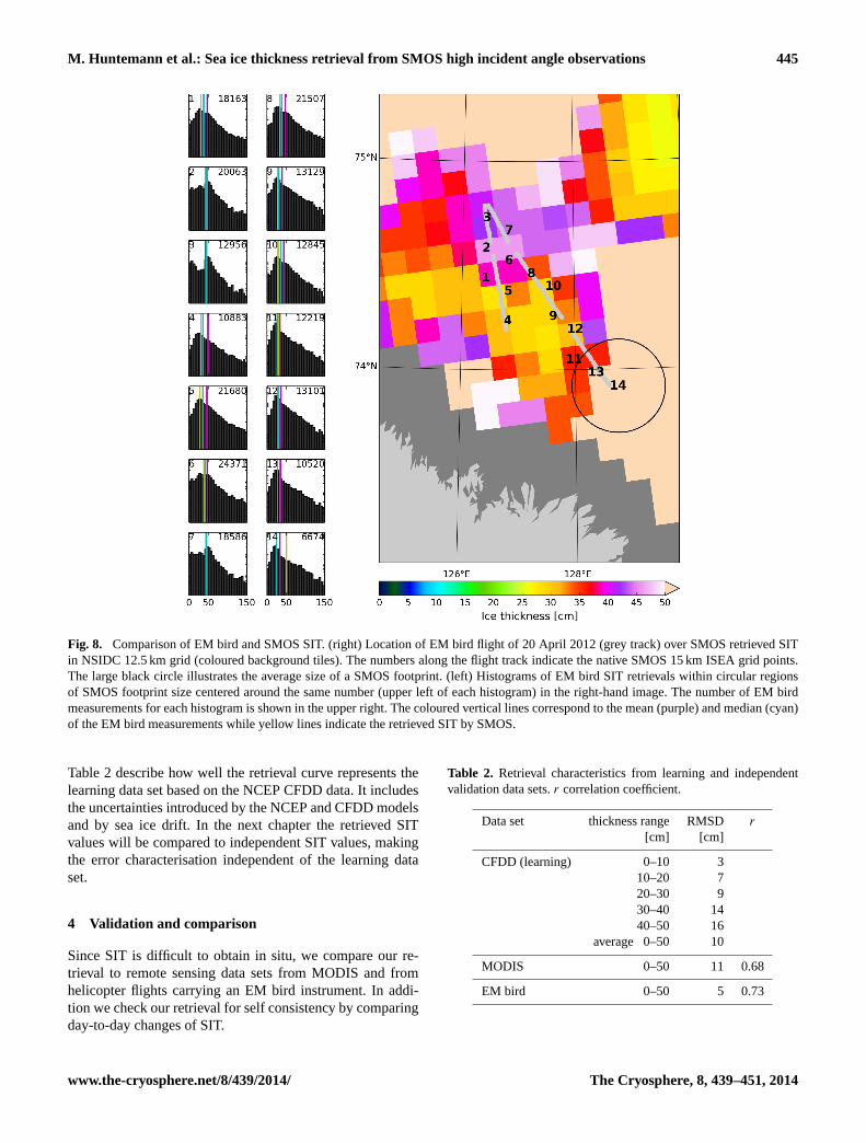
Fig. 8. Comparison of EM bird and SMOS SIT. (right) Location of EM bird flight of 20 April 2012 (grey track) over SMOS retrieved SITin NSIDC 12.5 km grid (coloured background tiles). The numbers along the flight track indicate the native SMOS 15 km ISEA grid points.The large black circle illustrates the average size of a SMOS footprint. (left) Histograms of EM bird SIT retrievals within circular regionsof SMOS footprint size centered around the same number (upper left of each histogram) in the right-hand image. The number of EM birdmeasurements for each histogram is shown in the upper right. The coloured vertical lines correspond to the mean (purple) and median (cyan)of the EM bird measurements while yellow lines indicate the retrieved SIT by SMOS.

Table2 describe how well the retrieval curve represents thelearning data set based on the NCEP CFDD data. It includesthe uncertainties introduced by the NCEP and CFDD modelsand by sea ice drift. In the next chapter the retrieved SITvalues will be compared to independent SIT values, makingthe error characterisation independent of the learning dataset.

4 Validation and comparison

Since SIT is difficult to obtain in situ, we compare our re-trieval to remote sensing data sets from MODIS and fromhelicopter flights carrying an EM bird instrument. In addi-tion we check our retrieval for self consistency by comparingday-to-day changes of SIT.

Table 2. Retrieval characteristics from learning and independentvalidation data sets.r correlation coefficient.

Data set thickness range RMSD r

[cm] [cm]

CFDD (learning) 0–10 310–20 720–30 930–40 1440–50 16

average 0–50 10

MODIS 0–50 11 0.68

EM bird 0–50 5 0.73

www.the-cryosphere.net/8/439/2014/ The Cryosphere, 8, 439–451, 2014

446 M. Huntemann et al.: Sea ice thickness retrieval from SMOS high incident angle observations

Fig. 9. Scatter plot of EM bird versus SMOS SIT retrieval. Blue:regression line. RMSD between data and regression line: 5 cm, cor-relation ofr = 0.73.

4.1 Using MODIS thermal imagery SIT retrieval

MODIS based ice surface temperature together withHIRLAM atmospheric forcing data was used to estimate thinice thickness over the Barents and Kara seas through theice surface heat balance equation (Yu and Rothrock, 1996;Mäkynen, 2011; Mäkynen et al., 2013). The spatial resolu-tion of the MODIS ice thickness charts is 1 km and they showSIT values from 0 to 99 cm. Only nighttime MODIS data wasemployed. Thus, the uncertainties related to the effects of so-lar shortwave radiation and surface albedo were excluded.For the cloud masking of the MODIS data, in addition to thedifferent cloud tests (Frey et al., 2008), also manual methodswere used in order to improve detection of thin clouds andice fog. In the SIT chart calculation, an average snow thick-ness vs. ice thickness relationship was used (Mäkynen et al.,2013). This relationship is based on an empirical relationshipbetween snow and ice thickness byDoronin (1971) and theSoviet Union’s Sever expeditions data (NSIDC, 2004). Thetypical maximum reliable SIT (max 50 % uncertainty) for theMODIS data was estimated to be 35–50 cm under typicalweather conditions (air temperature< −20◦C, wind speed5 m s−1). The accuracy is the best for the 15–30 cm thicknessrange, with an error of around 38 %. These figures are basedon the Monte Carlo method using estimated or guessed stan-dard deviations and covariances of the input variables to theSIT retrieval. No in situ data were available for the MODISSIT accuracy estimation.

Since originally MODIS has a much higher spatial reso-lution than SMOS, the MODIS data were averaged to theSMOS resolution. Another smaller discrepancy between thetwo data sets is that, when calculating the SMOS SIT, thedata of one day is averaged while the MODIS data stem fromsingle overflights.

The SMOS and MODIS SIT retrievals for one single day,4 December 2010, are shown in Fig.7 (top left and top cen-tre, respectively). The MODIS image shows incomplete cov-erage due to clouds. Some regions like northwest of NovayaZemlya show a good agreement in shape and thickness dis-tribution of the sea ice. In the image centre, east and southof the northeastern tip of Novaya Zemlya, SMOS retrieveshigher SIT values than MODIS. Areas closer to the coastthan 40 km are screened out because of potential land influ-ence in the SMOS data. In Fig.7 (top right) the averagedMODIS SIT values suitable for comparison with SMOS SITare shown.

Similar analyses have been performed for all days with asufficient number of coincident SMOS and MODIS thick-ness retrievals from 24 November to 14 April 2011 with 71scenes in total (not shown here). Figure7 (bottom) showsthe combined scatter plot. As the data have been taken undera variety of different conditions, the scatter is considerablylarge with a correlation ofr = 0.68 and a RMSD with respectto the regression line of 11 cm. The line has a slope of 1.75,indicating that on average the SMOS retrieval gives 75 %higher SIT than the MODIS retrieval. As a consequence, thetwo retrievals agree best at low thickness. The regressionline has been determined by minimising the RMSD to theMODIS retrievals.

For the assessment of the comparison with MODIS de-rived SIT, it should be kept in mind that the MODIS SITyields errors of mostly 40–50 % (Mäkynen et al., 2013).While the example shows good agreement of SIT from bothsensors below 20 cm thickness which supports the conclu-sion of lower errors in this range (Table2), we cannot at-tribute the statistic disagreement at higher thicknesses to anyof the two sensors. In addition, the errors in the two retrievalsstem from different sources. While the SMOS brightnesstemperatures are expected to have a higher random error dueto lower radiometric accuracy and averaging over a large in-cident angle range as the atmosphere is close to transparentin the L band, MODIS ice surface temperature may be influ-enced by thin clouds and fog missed by the MODIS cloudmask.

4.2 Using EM bird airborne measurements

The AWI has developed an airborne instrument to measureSIT when attached to a plane or helicopter (Haas et al., 2009),called EM bird. The method employs the contrast in electri-cal conductivity between sea water and sea ice for determin-ing the distance to the ice–water interface, and from a laseraltimeter the distance to the ice top. The difference yields

The Cryosphere, 8, 439–451, 2014 www.the-cryosphere.net/8/439/2014/

M. Huntemann et al.: Sea ice thickness retrieval from SMOS high incident angle observations 447D

iscussionPaper

|D

iscussionPaper

|D

iscussionPaper

|D

iscussionPaper

|

Fig. 10. Difference map of SMOS SIT retrieval from 20 to 21 Oct 2011 in the ice growth phase (left).Areas of open water and areas where the retrievals 50+ cm flag is set are excluded. Histogram of day today change from 20 to 21 Oct 2011 (top right). OSI-SAF sea ice displacement product from 19 to 21 Oct2011 (bottom right).

33

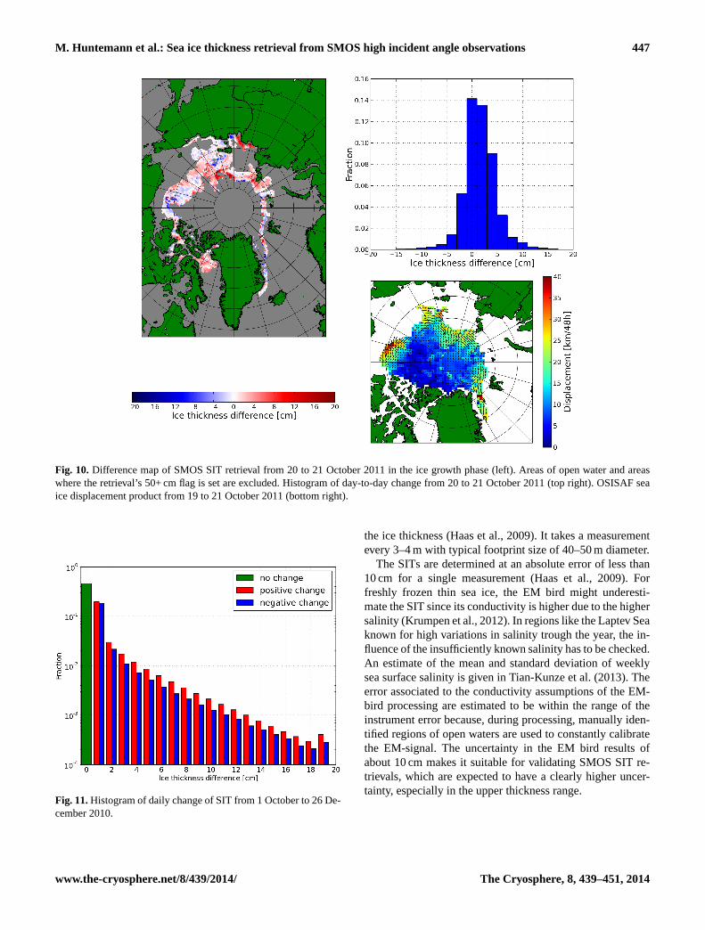
Fig. 10.Difference map of SMOS SIT retrieval from 20 to 21 October 2011 in the ice growth phase (left). Areas of open water and areaswhere the retrieval’s 50+ cm flag is set are excluded. Histogram of day-to-day change from 20 to 21 October 2011 (top right). OSISAF seaice displacement product from 19 to 21 October 2011 (bottom right).

Fig. 11.Histogram of daily change of SIT from 1 October to 26 De-cember 2010.

the ice thickness (Haas et al., 2009). It takes a measurementevery 3–4 m with typical footprint size of 40–50 m diameter.

The SITs are determined at an absolute error of less than10 cm for a single measurement (Haas et al., 2009). Forfreshly frozen thin sea ice, the EM bird might underesti-mate the SIT since its conductivity is higher due to the highersalinity (Krumpen et al., 2012). In regions like the Laptev Seaknown for high variations in salinity trough the year, the in-fluence of the insufficiently known salinity has to be checked.An estimate of the mean and standard deviation of weeklysea surface salinity is given inTian-Kunze et al.(2013). Theerror associated to the conductivity assumptions of the EM-bird processing are estimated to be within the range of theinstrument error because, during processing, manually iden-tified regions of open waters are used to constantly calibratethe EM-signal. The uncertainty in the EM bird results ofabout 10 cm makes it suitable for validating SMOS SIT re-trievals, which are expected to have a clearly higher uncer-tainty, especially in the upper thickness range.

www.the-cryosphere.net/8/439/2014/ The Cryosphere, 8, 439–451, 2014

448 M. Huntemann et al.: Sea ice thickness retrieval from SMOS high incident angle observations

On 20 April 2012 EM bird measurements were taken dur-ing a helicopter flight in the Laptev Sea over freshly frozenthin sea ice with negligible snow cover, shown in Fig.8 to-gether with the SMOS retrieved SIT.

The considerable variability of the EM bird ice thick-nesses within one single SMOS grid cell is shown in thehistograms on the left. As the meteorological conditions ofice formation should have been quite homogeneous withinthe SMOS footprints during the short lifetime of this thinice, the variability of ice thickness at this small horizontalscale should mainly be caused by mechanical redistributionof ice through the process of ridging, rafting, and shearing,as it has been documented for ice thicker than approximately2 m byWadhams(1983, 1992), finding exponential distribu-tions. Here, the logarithmic representation of the histogramsreveals similar exponential distributions also for sea ice inthe thickness range from 0.5 to 1.5 m. Close to the turningpoint of the helicopter (points 2, 3, 6, and 7) the SMOS re-trievals are around 45 cm (purple), and those from the EMbird are mainly above 50 cm thickness but also contain afew thin values of around 10 cm, possibly caused by leadsmuch smaller than the SMOS footprint size (see black circlein Fig. 8 (right) for an example). Since the EM bird mea-surements and the corresponding averages are taken along anarrow line of its footprints of 40–50 m width, but the SMOSfootprint covers a large area of about 50 km in diameter, wehave to expect larger discrepancies in the SIT retrievals fromthe two instruments. The fraction of SMOS footprint areacovered by EM bird measurements along one flight track isabout 0.1 % or less. The coloured vertical lines in the his-tograms in Fig.8 correspond to the mean (purple) and me-dian (cyan) of all EM bird measurements within the corre-sponding SMOS footprint. The yellow lines indicate the re-trieved SIT by SMOS. In almost all cases the SMOS retrievalagrees better with the median because it is less influenced bythe long tail of high thickness values in the distribution. Theonly case of larger disagreement is histogram 14, where theEM bird median thickness is 25 cm and the SMOS thicknessexceeds its limit of 50 cm. This is in agreement with the mapin Fig. 8 (right) where the SMOS SIT mostly exceeds 50 cmwithin the size of a footprint (black circle) around point 14.Apparently these thick ice regions are missed by the EM birdmeasurements (small gray dots) as can be seen in the his-togram. This is an example for the more general case whereparts of the SMOS footprint are covered by ice thicker thanSMOS can retrieve. Therefore, this case is excluded from thecomparison in Fig.9. The histogram of point 3 near the turn-ing point of the flight shows a pronounced bi-modal shape in-dicating at least two different regimes of ice thickness withinthis SMOS footprint. As the EM bird thicknesses in Fig.8are the best large-scale in situ observations of thin sea ice wecurrently have, we perform the comparison in the scatter plotof Fig. 9 in spite of the small number of data points from aquite limited region and season entering the comparison. The

diagram shows a good agreement with correlation coefficientr = 0.73 and RMSD of 5 cm.

4.3 Day-to-day differences – plausibility check

The two preceding sections have shown the limitedness inspace, time and sea ice thickness of validation data avail-able to us. Therefore, as an additional, more global consis-tency check the SIT difference of two consecutive days, 20and 21 October 2011, was investigated (Fig.10, left). As thethermodynamic thickness growth within one day is limited,large changes are either due to drift or errors in the retrieval.In most regions of the map the change is a few centimetres.In the Beaufort Sea (75◦ N, 140◦ W), narrow parallel bandsof opposite sign in SIT difference indicate sea ice drift whichis confirmed by the vectors (Fig.10, bottom right) of the seaice drift product from the OSI-SAF (Lavergne et al., 2010)running perpendicular to the bands of high sea ice thicknesschange. Other regions of high thickness change are foundnear the upper limit of the retrieved sea ice thicknesses wherethe retrieval noise is higher, extending e.g. east of northernGreenland, and north of Svalbard and Franz Josef Land. Thestrong increase in thickness in the Laptev Sea is in goodagreement with CFDD based modelled growth of very thinice at temperatures of around−10◦C.

Figure 11 provides histograms of all positive (red) andnegative (blue) day-to-day changes from October to Decem-ber 2010. The plausible changes between±1 cm occur mostfrequently. This range covers about 90 % of all pixels. Nega-tive changes of 1 cm thickness are considered plausible herebecause of the uncertainty of the retrieval procedure. Accord-ing to the overall sea ice increase in the freezing season, in alldays the positive changes overbalance the negative ones. Theaverage daily increase in SIT is 0.3 cm with a standard de-viation of 3.3 cm reflecting the average ice thickness changethroughout the Arctic. Higher changes in SIT than±8 cmare detected in less than 0.5 % of the cases. Such strong icethickness changes will not be generated thermodynamicallybut are drift or other disturbing influences, as, according toEq. (2), an ice thickness growth from, e.g. 2 to 10 cm withinone day requires an air temperature of−30◦C. In conclu-sion, the SMOS data generally provides a realistic scenariofor a daily ice thickness development in the Arctic during thefreeze-up period.

5 Discussion and conclusions

An empirical retrieval of SIT in the freeze-up period using Lband (1.4 GHz) brightness temperatures of sea ice acquiredby SMOS has been developed. The retrieval is trained by aCFDD based model in the Kara and Barents seas during thefreeze-up period and uses intensity (the average of horizon-tally and vertically polarised brightness temperatures) as well

The Cryosphere, 8, 439–451, 2014 www.the-cryosphere.net/8/439/2014/

M. Huntemann et al.: Sea ice thickness retrieval from SMOS high incident angle observations 449

as the polarisation difference at incidence angles between 40and 50◦.

Table 2 concludes the calibration and validation errorsfrom the various sources. The calibration data set reveals astrong increase of the retrieval error from 3 cm for thicknessbelow 10–16 cm in the range from 40 to 50 cm thickness.The overall average error is 10 cm. The two comparison datasets, based on MODIS and EM bird measurements, respec-tively, confirm the tendency of better retrievals for lower icethickness. However, as both data sets are sparse, we onlygive overall retrieval errors. They are 11 and 5 cm, respec-tively. Compared to the average error of the learning data set(10 cm) these values appear quite optimistic which may beexplained by the small size, the homogeneity and the spe-cific thickness distribution of the validation data sets. As theretrieval error increases with thickness, the actual error ofany validation data set will depend on its thickness distribu-tion, with higher errors for thicker ice. In Arctic-wide appli-cations, we have to expect the average thickness towards thehigh end of the retrieval range of 0–50 cm as the ice growthrate decreases with thickness (Eq.2). The most accurate val-idation data is the AWI EM bird sea ice thicknesses observa-tions. Here, the correlation with the SMOS based thicknessis 0.73 while the correlation between the example of MODISand SMOS based retrievals is 0.68, again supporting the sug-gested method.

It should be noted that the thickness range retrieved here isonly found during the freeze-up season. During melt, the seaice cover is too inhomogeneous for this method to be applied,with the mixture of wet sea ice, melt ponds and open water tobe expected within one SMOS footprint. As a consequence,the method is applicable, as a rule of thumb, in the Arcticfrom October to April and in the Antarctic from March to Oc-tober. Even during this time, melt or rain events may also leadto single misleading results. However, the comparison withthe MODIS based thicknesses presented in the scatter plot ofFig. 7 covers the complete season from November 2010 toApril 2011 in a statistically representative way.

As the validation studies indicate a good agreement be-tween the two investigated data sets, further investigation toexplain and understand this relationship using a microwaveemission model is desirable. This will specifically aim toquantify the additional influence of temperature, salinity andwind speed on intensity and polarisation difference.

Sensitivity studies with a radiative bulk sea ice modelshow little increase of intensity with increasing temperatureand salinity (Maaß, 2013). The polarisation difference alsoincreases little with salinity, but more with temperature whenit approaches melting. At higher ice thickness under freezingconditions (for which the algorithm is intended), we expectlower ice temperatures, where the temperature influence onthe polarisation difference is again small.

Snow is nearly transparent at L band, but a noticeable ef-fect is expected from the indirect influence of snow by ther-mal insulation, leading to higher ice temperatures, and thus

to higher polarisation difference, increased brine volume,higher permittivity and thinner thickness retrievals (Fig.6).We thus expect the strongest influences on the retrieval fromtemperature and snow cover and we suggest these should beinvestigated further. However, as the method presented hereis completely empirical, the mentioned influences should au-tomatically be included in a statistical way, e.g. a snow coverincreasing statistically as the ice ages and becomes thicker.As the present study shows, even without taking these influ-ences into account, the retrieval works within the indicatedlimits. Discrepancies can be expected if applied in regionswith much snowfall, e.g. in the Pacific sector of the SouthernOcean where the algorithm has been applied successfully, too(not shown here). Another restriction of the algorithm is theassumption of 100 % SIC. While attempts to include SIC as asecond parameter into the retrieval have turned out to be verysensitive to noise of the input data (Sect. 3), restricting the re-trieval to near 100 % sea ice cover (obtained from other pas-sive microwave sensors) could improve the accuracy of theretrieval. However, the focus of this study is a single-sensorretrieval.

Since SMOS brightness temperatures are quite sensitiveto the incidence angle in the range of 40–50◦ (Fig. 1), weare currently working on improving the retrieval by using theincidence angle as an explicit parameter.

The present retrieval and that suggested byKaleschke et al.(2012) use different, independently taken data as they usedisjoint incidence angle ranges (0–40◦ vs. 40–50◦). In future,both retrievals could be combined, e.g. by fitting an analyt-ical curve to the observations of all incidence angles withinone grid cell and then determining the ice thickness from theparameters of that curve.

In the training, only thermodynamic and no dynamic icegrowth in the Kara Sea and Barents Sea is assumed. Onepossibility to exclude ice thickness changes by drift from alearning data set would be to use a fast ice region, e.g. inthe Laptev Sea. However, using such a data set would riskleading one to a retrieval biased towards the characteristicsof undeformed ice.

Another sensor observing sea ice thickness since 2012 isCryoSat2 (Laxon et al., 2013). While SMOS is sensitive tothin ice thickness only, the altimeter CryoSat2 has the highestuncertainty for thin sea ice and is more accurate for thickersea ice of more than 1 m. Comparing spatial distributions ofice thicknesses from both sensors can serve as another con-sistency check, and, if successful, a combined data productcould cover a larger thickness range than each single one ofthe two sensors. However, such comparison and combinationwill have to be done on the base of monthly averages becausea daily data product of CryoSat2 sea ice thicknesses is cur-rently not available.

www.the-cryosphere.net/8/439/2014/ The Cryosphere, 8, 439–451, 2014

450 M. Huntemann et al.: Sea ice thickness retrieval from SMOS high incident angle observations

Acknowledgements.Financial support of the European SpaceAgency (ESA) project SMOSIce, contract no. 4000101476, theEU project Sea Ice Downstream services for Arctic and AntarcticUsers and Stakeholders (SIDARUS), grant agreement 262922 andFederal Ministry of Education and Research/Bundesministeriumfür Bildung und Forschung (BMBF) MiKliP project Climate ModelValidation by confronting globally Essential Climate Variablesfrom models with observations (ClimVal) is gratefully acknowl-edged. The authors thank the National Centers for EnvironmentalPrediction (NCEP) for data provision and the editor and reviewersfor their helpful comments which greatly improved the quality.

Edited by: J. Stroeve

References

Bilello, M.: Formation, growth, and decay of sea-ice in the Cana-dian Arctic Archipelago, Arctic, 1961.

Brown, M., Torres, F., Corbella, I., and Colliander, A.: SMOS Cali-bration, IEEE Transactions on Geoscience and Remote Sensing,46, 646–658, doi:10.1109/TGRS.2007.914810, 2008.

Camps, A., Gourrion, J., Tarongi, J. M., Gutierrez, A., Barbosa, J.,and Castro, R.: RFI Analysis in SMOS Imagery, in: Geoscienceand Remote Sensing Symposium (IGARSS proceedings 2010),2007–2010, 2010.

Castro, R.: Analytical Pixel Footprint, Tech. rep., availableat: http://www.smos.com.pt/downloads/release/documents/SO-TN-DME-L1PP-0172-Analytical-Pixel-Footprint.pdf(lastaccess: 17 March 2014), 2008.

Corbella, I., Duffo, N., Vall-llossera, M., Camps, A., and Torres,F.: The visibility function in interferometric aperture synthesisradiometry, IEEE Trans. Geosci. Remote Sens. 42, 1677–1682,doi:10.1109/TGRS.2004.830641, 2004.

Doronin, Y. P.: Thermal Interaction of the Atmosphere and Hydro-sphere in the Arctic, Isr. Program for Sci. Transl., Jerusalem,1971.

Frey, R. a., Ackerman, S. A., Liu, Y., Strabala, K. I., Zhang,H., Key, J. R., and Wang, X.: Cloud Detection withMODIS. Part I: Improvements in the MODIS Cloud Maskfor Collection 5, J. Atmos. Ocean. Technol., 25, 1057–1072,doi:10.1175/2008JTECHA1052.1, 2008.

Fuhrhop, R., Grenfell, T., and Heygster, G.: A combined radiativetransfer model for sea ice, open ocean, and atmosphere, RadioScience, 33, 303–316, doi:10.1029/97RS03020, 1998.

Haas, C., Lobach, J., Hendricks, S., Rabenstein, L., and Pfaffling,A.: Helicopter-borne measurements of sea ice thickness, using asmall and lightweight, digital EM system, J. Appl. Geophys., 67,234–241, doi:10.1016/j.jappgeo.2008.05.005, 2009.

Heygster, G., Huntemann, M., and Wang, H.: Algorithm Theo-retical Basis Document (ATBD) for the University of BremenPolarization-based SMOS sea ice thickness retrieval algorithm(Algorithm II), Tech. Rep. Algorithm II, Institute of Environmen-tal Physics, Bremen, Germany, 2012.

Kaleschke, L., Maaß, N., Haas, C., Hendricks, S., Heygster, G., andTonboe, R. T.: A sea-ice thickness retrieval model for 1.4 GHzradiometry and application to airborne measurements over lowsalinity sea-ice, The Cryosphere, 4, 583–592, doi:10.5194/tc-4-583-2010, 2010.

Kaleschke, L., Tian-Kunze, X., Maaß, N., Mäkynen, M., and Dr-usch, M.: Sea ice thickness retrieval from SMOS brightness tem-peratures during the Arctic freeze-up period, Geophys. Res. Lett.,39, L05501, doi:10.1029/2012GL050916, 2012.

Källen, E.: HIRLAM Documentation Manual, System 2.5, Tech.rep., Swed. Meteorol. and Hydrol. Inst, Norrköping, Sweden,1996.

Kalnay, E., Kanamitsu, M., Kistler, R., Collins, W., Deaven, D.,Gandin, L., Iredell, M., Saha, S., White, G., Woollen, J., Zhu, Y.,Leetmaa, A., Reynolds, R., Chelliah, M., Ebisuzaki, W., Higgins,W., Janowiak, J., Mo, K. C., Ropelewski, C., Wang, J., Jenne, R.,and Joseph, D.: The NCEP/NCAR 40-Year Reanalysis Project,Bull. Am. Meteorol. Soc., 77, 437–471, doi:10.1175/1520-0477(1996)077<0437:TNYRP>2.0.CO;2, 1996.

Kern, S., Spreen, G., Kaleschke, L., Rosa, S. D. E. L. A., and Heyg-ster, G.: Polynya Signature Simulation Method polynya area incomparison to AMSR-E 89 GHz sea-ice concentrations in theRoss Sea and off lie Coast, Antarctica, for 2002–05 : first resultsthe Ade, 409–418, doi:10.3189/172756407782871585, 2007.

Kerr, Y., Waldteufel, P., Wigneron, J.-P., Martinuzzi, J., Font, J., andBerger, M.: Soil moisture retrieval from space: the Soil Moistureand Ocean Salinity (SMOS) mission, IEEE Trans. Geosci. Re-mote Sens., 39, 1729–1735, doi:10.1109/36.942551, 2001.

Krumpen, T., Hedricks, S., and Haas, C.: Data report on EM-Birdice thickness measurements for SMOSIce validation obtainedduring Transdrift XX, ARK XXVII/3 and SafeWin 2011 cam-paigns, Tech. rep., Alfred Wegener Institute for Polar and MarineResearch, Bremerhaven, Germany, 2012.

Kwok, R., Comiso, J. C., Martin, S., and Drucker, R.: RossSea polynyas: Response of ice concentration retrievals tolarge areas of thin ice, J. Geophys. Res., 112, C12012,doi:10.1029/2006JC003967, 2007.

Launiainen, J. and Cheng, B.: Modelling of ice thermodynamicsin natural water bodies, Cold Reg. Sci. Technol., 27, 153–178,1998.

Lavergne, T., Eastwood, S., Teffah, Z., Schyberg, H., and Breivik,L.-a.: Sea ice motion from low-resolution satellite sensors: Analternative method and its validation in the Arctic, J. Geophys.Res., 115, C10032, doi:10.1029/2009JC005958, 2010.

Laxon, S. W., Giles, K. A., Ridout, A. L., Wingham, D. J., Willatt,R., Cullen, R., Kwok, R., Schweiger, A., Zhang, J., Haas, C.,Hendricks, S., Krishfield, R., Kurtz, N., Farrell, S., and Davidson,M.: CryoSat-2 estimates of Arctic sea ice thickness and volume,Geophys. Res. Lett., 40, 732–737, doi:10.1002/grl.50193, 2013.

Maaß, N.: Remote sensing of sea ice thickness using SMOS data,Ph.D. thesis, 2013.

Mäkynen, M.: STSE-SMOS Sea Ice Retrieval Study SMOSIce WP3 Assembly of the SMOSIce Data Base SMOSIce-DAT usermanual for the validation data Deliverable D-6b Draft EURO-PEAN SPACE AGENCY STUDY CONTRACT REPORT UnderESTEC Contract No. 4000101476/10/NL/CT, Tech. rep., 2011.

Mäkynen, M., Cheng, B., and Simila, M.: On the accuracyof thin-ice thickness retrieval using MODIS thermal im-agery over Arctic first-year ice, Ann. Glaciol., 54, 87–96,doi:10.3189/2013AoG62A166, 2013.

Mecklenburg, S., Drusch, M., Kerr, Y. H., Font, J., Martin-Neira, M., Delwart, S., Buenadicha, G., Reul, N., Daganzo-Eusebio, E., Oliva, R., and Crapolicchio, R.: ESA’s Soil Mois-ture and Ocean Salinity Mission: Mission Performance and Op-

The Cryosphere, 8, 439–451, 2014 www.the-cryosphere.net/8/439/2014/

M. Huntemann et al.: Sea ice thickness retrieval from SMOS high incident angle observations 451

erations, IEEE Trans. Geosci. Remote Sens., 50, 1354–1366,doi:10.1109/TGRS.2012.2187666, 2012.

NSIDC: Morphometric characteristics of ice and snow in the Arc-tic Basin: aircraft landing observations from the Former SovietUnion, 1928–1989, Compiled by I. P. Romanov, Boulder, CO:National Snow and Ice Data Center, Digital medi., 2004.

Oliva, R., Daganzo, E., Kerr, Y. H., Mecklenburg, S., Ni-eto, S., Richaume, P., and Gruhier, C.: SMOS Radio Fre-quency Interference Scenario: Status and Actions Taken toImprove the RFI Environment in the 1400–1427-MHz Pas-sive Band, IEEE Trans. Geosci. Remote Sens., 50, 1427–1439,doi:10.1109/TGRS.2012.2182775, 2012.

Sahr, K., White, D., and Kimerling, A. J.: Geodesic Discrete GlobalGrid Systems, Cartography and Geographic Information Sci-ence, 30, 121–134, doi:10.1559/152304003100011090, 2003.

Sakov, P., Counillon, F., Bertino, L., Lisæter, K. A., Oke, P. R., andKorablev, A.: TOPAZ4: an ocean-sea ice data assimilation sys-tem for the North Atlantic and Arctic, Ocean Sci., 8, 633–656,doi:10.5194/os-8-633-2012, 2012.

Spreen, G., Kaleschke, L., and Heygster, G.: Sea ice remote sens-ing using AMSR-E 89-GHz channels, J. Geophys. Res., 113,C02S03, doi:10.1029/2005JC003384, 2008.

Tian-Kunze, X., Kaleschke, L., Maaß, N., Mäkynen, M., Serra, N.,Drusch, M., and Krumpen, T.: SMOS derived sea ice thickness:algorithm baseline, product specifications and initial verifica-tion, The Cryosphere Discuss., 7, 5735–5792, doi:10.5194/tcd-7-5735-2013, 2013.

Tonboe, R. T., Dybkjaer, G., and Høyer, J. L.: Simulations of thesnow covered sea ice surface temperature and microwave effec-tive temperature, Tellus A, 63, 1028–1037, doi:10.1111/j.1600-0870.2011.00530.x,2011.

Unden, P., Rontu, L., Järvinen, H., and Lynch, P.: HIRLAM-5 scientific documentation, available at:http://citeseerx.ist.psu.edu/viewdoc/summary?doi=10.1.1.6.3794(last access:17 March 2014), 2002.

Wadhams, P.: Sea ice thickness distribution in Fram Strait, Nature,305, 108–111, doi:10.1038/305108a0, 1983.

Wadhams, P.: Sea ice thickness distribution in the Greenland Seaand Eurasian Basin, May 1987, J. Geophys. Res., 97, 5331,doi:10.1029/91JC03137, 1992.

Weeks, W.: On Sea Ice, University of Alaska Press, 2010.Yu, Y. and Rothrock, D. A.: Thin ice thickness from satel-

lite thermal imagery, J. Geophysi. Res., 101, 25753–25766,doi:10.1029/96JC02242, 1996.

Zine, S., Boutin, J., Font, J., Reul, N., Waldteufel, P., Gabarro, C.,Tenerelli, J., Petitcolin, F., Vergely, J.-L., Talone, M., and Del-wart, S.: Overview of the SMOS Sea Surface Salinity Proto-type Processor, IEEE Trans. Geosci. Remote Sens., 46, 621–645,doi:10.1109/TGRS.2008.915543, 2008.

www.the-cryosphere.net/8/439/2014/ The Cryosphere, 8, 439–451, 2014