ELR 4202CMEDICAL INSTRUMENTATION LABORATORY

H. WATSONSPRING, 2008

M. HEIMERFALL, 2007

GENERAL INSTRUCTIONS

1. THE LABORATORY PROCEDURE

Assign one team member to record measured data while others work with the hardware. These roles should be rotated so all team members get “hands on” experience.Record all measurements in a bound notebook. Be sure to identify all instruments you used in the procedure (the manufacturer and model as well as the serial number).Record in the laboratory notebook descriptions of all procedures carried out. You should also make notations of observations and any conclusions based on the results.

2. THE LAB REPORT

The lab report is due one week after the procedure is completed. The cover page must list the course title, the date, names of the team members and a title for the lab. The Table of Contents lists the first page number for all sections. The Procedure section will describe the steps taken, the data that was recorded and observations about the results. Questions posed in the lab handout should be answered within this section and/or in the Conclusions section. The Conclusions section will summarize the lab procedure. Some of the questions posed in the handout will be answered in this section. It should also include a section labeled “lessons learned” that describes the skills and knowledge gained from completing the lab. The Appendix should contain a photo-copy of the original entries in the lab notebook.

SCHEDULE

DATE TEAMS 1, 2 & 3 TEAMS 4, 5 & 6

Week 1 LAB ORIENTATION LAB ORIENTATION

Week 2 LAB #1 LAB #3

Week 3 LAB #2 LAB #4

Week 4 LAB #3 LAB #1

Week 5 LAB #4 LAB #2

Page 1

ELR 4202C

LABORATORY #1

I. Layout of “proto-board”

The breadboard used in this procedure allows a circuit to be fabricated by inserting components into the socket holes. The figure on the next page shown the connections that exist between some of the socket holes. The terminology for this lab: the long rows of holes (marked by red and blue stripes) are called “bus strips”. The “groups of 5” are the short columns of holes on both sides of a central “gutter”.

Verifying the board connections:

Take a resistor and insert both ends into holes on the same bus strip. Set the digital meter to “ohms”, touch the probes to both ends of the resistor and record the resistance reading. Move one end of the resistor to the other bus strip and repeat the measurement. Leave one end in a bus strip and move the other end to one of the groups of 5 holes and repeat the measurement. Remove the resistor and place both ends into holes within the same groups of 5. Measure the resistance between the ends. Move one end of the resistor to the group on the other side of the gutter and repeat. Does this verify the proto-board interconnections shown in the figure?

II. Measure resistors

The resistors used in this laboratory are either metal film or carbon film. They are manufactured by depositing the thin film on a cylindrical insulator and etching a helical pattern to attain the proper resistance. It is then covered with a resin and painted with a color code to indicate its nominal resistance value. The gold band indicates that these resistors have a tolerance of ±5% from the nominal value. These resistors have a power rating of ¼ watt. Obtain a copy of the resistor color code and use it to evaluate the resistor values in this procedure.

Your team has been given ten resistors: five each of two different values. Determine the nominal resistance values by interpreting the color code. Insert the resistors into the board and measure their exact values. Calculate the deviation from the nominal values and compare this to the ±5% guaranteed by the manufacturer. Do all of the resistors meet specifications?

Page 2

Page 3

III. DC resistor circuits

Set the digital meter to the DC volts mode and connect the probes to the output terminals of the power supply. Set the voltage to exactly 5.00 volts. Is there any discrepancy between the external meter and the meter in the power supply? If so, that is the percentage difference?

Turn off the voltage and connect the power supply to bus strips along the top and bottom edges of the board. Use a combination of the connections in the board and jumper wires to create the circuit shown below.

Turn on the power supply and measure the voltage (referenced to ground) on node A. Repeat for node B. For both cases, reduce the circuit to a 2-resistor voltage divider circuit by using the equations for series and parallel resistors. (For node A, the three resistors between node A and ground will be reduced to a single resistance.) Calculate the node voltages using the voltage divider formula and compare them to the measurements. Is the difference within the resistor tolerance?

Remove a jumper wire to open the circuit at either node A or node B. Set the meter to DC current mode and connect the probes to complete the opened circuit. Record the measured current and compare it to the calculated value. Is the difference within the resistor tolerance?

IV. R-C low pass filter circuit

Remove the DC power supply connection to the board. Turn on the signal generator and the oscilloscope. Connect the oscilloscope input to the output terminals of the signal generator. Set the signal generator to the sinusoidal mode and a frequency of 500 Hz. Adjust the output amplitude to 10 volts, peak-to-peak.

Page 4

Connect the signal and ground from the signal generator to the top and lower bus strips previously connected to the DC power supply.Insert a 10 Kilohm resistor and a 15 nanofarad capacitor to create the circuit shown below.

Set the oscilloscope to the 2-channel mode. Connect the top channel to the VS from the signal generator and the lower channel to the VOUT signal.

Classify this filtering circuit as either high pass or low pass and calculate the pole frequency in Hz. Sketch the Bode plot for this circuit based on the information covered in the lecture. Then, measure the response by observing the signals on the screen as the frequency is changed. Confirm that the input voltage on the upper trace has constant amplitude at all frequencies. Change the frequency over a range from 100 Hz to 10 Khz with three points per decade (e.g. 100, 200, 500, 1000, etc.). Take extra readings near the pole frequency to show more detail.

Calculate the gain in decibels at all frequencies and use this to generate a Bode plot. For the report, overlay both the calculated and measured Bode plots on the same graph and comment on the difference. Is it consistent with the tolerances of the resistor and capacitor values?

V. Windkessel Model

For the last part of this laboratory you will characterize a circuit that simulates part of the cardiovascular system by modifying the RC circuit in part IV. The resistors and capacitors simulate fluidic parameters. The results allow some insight into the hemodynamic response of the physiological system. The applied voltage (VS) will be a simulated aortic pressure waveform (AOP.tfw) that has been stored in the memory of the signal generator. To activate that waveform, do the following: 1. press ARBITRARY WAVEFORM button on front panel2. select ARB. WAVEFORM MENU3. select INTERNAL MEMORY

Page 5

4. select USER 1 using knob5. select OK

The following differential equation relates fluid flow (current) from a pump (the heart) into a flexible pipe (the aorta) and the aortic pressure (voltage) generated:

dt

tdPC

R

tPtI

)()()( +=

I(t) is the fluid flow out of the heart as a function of time measured in volume per time, P(t) is the water pressure as a function of time measured in force per area, C is equal to the ratio of pressure to volume, and R is the flow-pressure ratio. The same equation describes the relationship between the current, I(t), and the time-varying electric potential, P(t), in the following electrical circuit:

In terms of the physiological system, I(t) is the flow of blood from the heart to the aorta measured in cm3/sec, P(t) is the blood pressure in the aorta in mmHg, C is the arterial compliance in the aorta in cm3/mmHg, and R is the peripheral resistance in the systemic arterial system in mmHg.s/cm3.

Page 6

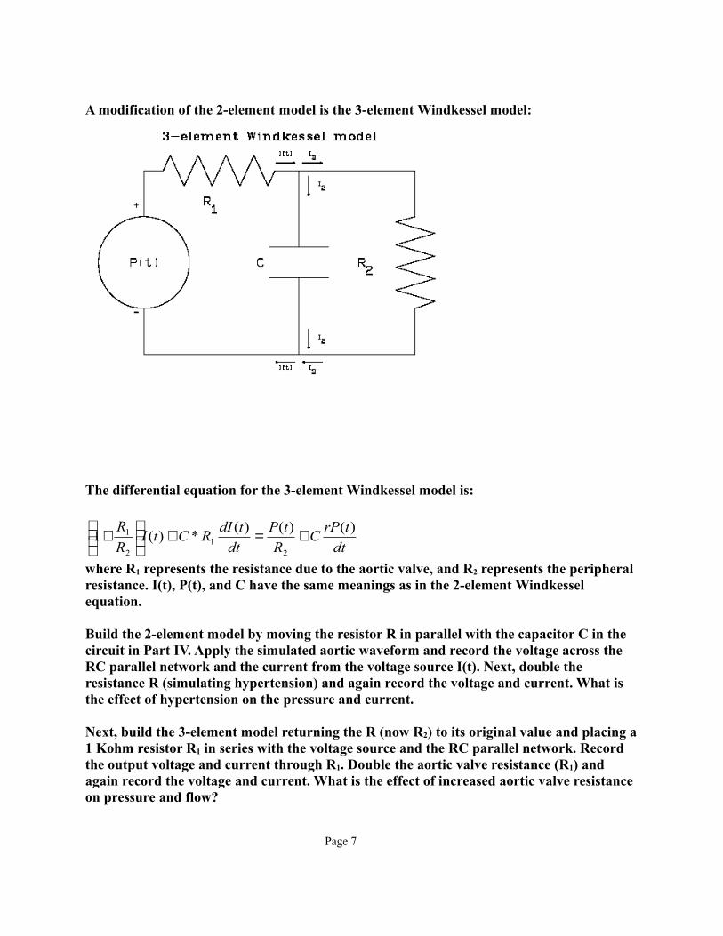
A modification of the 2-element model is the 3-element Windkessel model:

The differential equation for the 3-element Windkessel model is:

dt

trPC

R

tP

dt

tdIRCtI

R

R )()()(*)(1

21

2

1 +=+

+

where R1 represents the resistance due to the aortic valve, and R2 represents the peripheral resistance. I(t), P(t), and C have the same meanings as in the 2-element Windkessel equation.

Build the 2-element model by moving the resistor R in parallel with the capacitor C in the circuit in Part IV. Apply the simulated aortic waveform and record the voltage across the RC parallel network and the current from the voltage source I(t). Next, double the resistance R (simulating hypertension) and again record the voltage and current. What is the effect of hypertension on the pressure and current.

Next, build the 3-element model returning the R (now R2) to its original value and placing a 1 Kohm resistor R1 in series with the voltage source and the RC parallel network. Record the output voltage and current through R1. Double the aortic valve resistance (R1) and again record the voltage and current. What is the effect of increased aortic valve resistance on pressure and flow?

Page 7

ELR 4202CLABORATORY #2

M. HEIMERFALL, 2007

APPLICATIONS OF AN OP AMP AND 555 TIMER ICI. Characteristics and pin-outs of op amp and 555 ICs

Study the attached data sheets before the lab meeting. Mark up the schematic diagrams with the pin numbers that will be connected in the IC. Use the data sheet to design the 555 mono-stable circuit described in part V.

II. Connecting power to the op ampDesignate the bus strips on the proto-board that you will use for power and ground connections. It is suggested to use the red stipped bus for +5 volts and the blue stripped bus for -5 volts. Use a jumper to connect together the two inner bus strips and connect them to ground. Turn off the power supply and insert the op amp IC in the center of the board, bridging the gutter. Then insert jumpers to connect the power pins of the IC to the power buses.

III. Basic amplifier circuitsInsert resistors and jumpers to create the amplifier circuit shown below. Note that the signal generator connected with a series resistor of 10 kilohms simulates a signal source with high internal impedance.

Adjust the signal generator to produce a sinusoid at 100 Hz with a peak amplitude of ±100 millivolts and connect it to the board. Turn on the power supply and measure both VIN and VOUT. Based on these measurements, calculate the input impedance and the voltage gain for this circuit. Compare the measured gain to the calculate value. Increase the input signal amplitude to 200 mV, 500 mV and 1.0 volt. Record the VOUT waveform and calculate the gain for each input. Explain what happened and relate it to the VSAT parameter from the data sheet.Turn off the power and modify the board to this inverting amplifier circuit.

Page 8

Adjust the signal generator to ±100 mV, turn on the power and measure VIN and VOUT. Based on these measurements, calculate the input impedance and voltage gain of this circuit. Compare to the calculated values.

IV. ECG AmplifierTurn off the power and modify the circuit to the one shown below.

Insert the USB device into the signal generator so it produces the simulated ECG signal. Adjust the signal generator so the R-wave peak is 100 millivolts and the rate is 72 beats-per-minute. Note that this VECG signal simulates the signal from an instrumentation amplifier that is connected to bio-electrodes. Calculate the value for the capacitor C to produce a pole frequency of 500 Hz and insert the closest standard value into the board. Observe the signals at the input and output and calculate the voltage gain. Compare this to the expected voltage gain. Modify the value of C to create pole frequencies of 100 Hz, 50 Hz and 10 Hz. Capture both the input and output waveforms from the last trial and insert in your report. How does the R-wave from this last trial rate in terms of accuracy for clinical analysis?

Page 9

I. Detecting the R-wave

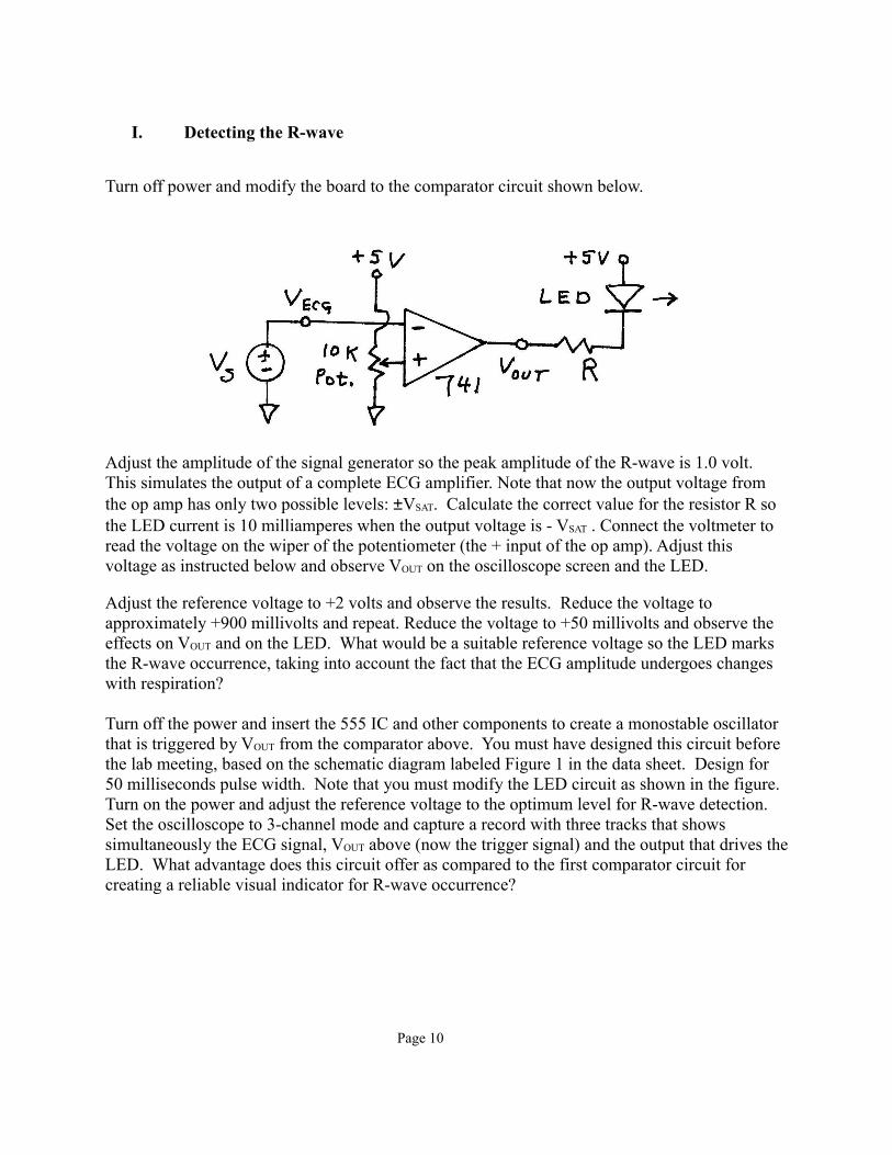
Turn off power and modify the board to the comparator circuit shown below.

Adjust the amplitude of the signal generator so the peak amplitude of the R-wave is 1.0 volt. This simulates the output of a complete ECG amplifier. Note that now the output voltage from the op amp has only two possible levels: ±VSAT. Calculate the correct value for the resistor R so the LED current is 10 milliamperes when the output voltage is - VSAT . Connect the voltmeter to read the voltage on the wiper of the potentiometer (the + input of the op amp). Adjust this voltage as instructed below and observe VOUT on the oscilloscope screen and the LED.

Adjust the reference voltage to +2 volts and observe the results. Reduce the voltage to approximately +900 millivolts and repeat. Reduce the voltage to +50 millivolts and observe the effects on VOUT and on the LED. What would be a suitable reference voltage so the LED marks the R-wave occurrence, taking into account the fact that the ECG amplitude undergoes changes with respiration?

Turn off the power and insert the 555 IC and other components to create a monostable oscillator that is triggered by VOUT from the comparator above. You must have designed this circuit before the lab meeting, based on the schematic diagram labeled Figure 1 in the data sheet. Design for 50 milliseconds pulse width. Note that you must modify the LED circuit as shown in the figure. Turn on the power and adjust the reference voltage to the optimum level for R-wave detection. Set the oscilloscope to 3-channel mode and capture a record with three tracks that shows simultaneously the ECG signal, VOUT above (now the trigger signal) and the output that drives the LED. What advantage does this circuit offer as compared to the first comparator circuit for creating a reliable visual indicator for R-wave occurrence?

Page 10

Page 11

Page 12

Page 13

Page 14

Page 15

ELR 4202CLABORATORY #3

Exercise I: Calibrate pH meter and optical O2 sensor.

pH Meter (Dr. Anthony McGoron)

1. There are three references solutions: pink (pH 4), yellow (pH 7), and blue (pH 10).

2. Clean the tip of the sensor using de-ionized water.

3. Dab the water off the sensor using tissue papers. Do not wipe the sensor forcefully.

4. Insert the sensor into one of the reference solutions.

5. When the display of the pH meter indicates ‘stable’ (i.e., stable reading), press the ‘STD’ button.

6. If the slope displayed on the screen is greater than 95%, then the calibration is successful.

7. Press the ‘STD’ bottom again.

8. Repeat the same process for the other two references

9. Upon completing the calibration process, store the sensor in the standard storing solution.

Optical O2 sensor (Dr. Wei-Chiang Lin)

Calibration Procedure

This procedure does not include temperature compensation as this not yet possible with dissolved oxygen measurements.

1. Prepare media with known O2 concentration level. The easiest concentrations will be atmospheric oxygen levels (20.9%) and zero. Zero oxygen is best attained by adding sodium dithionite to the solution. Make sure the media are maintained at a constant temperature level.

Page 16

2. Set data acquisition parameters for your calibration procedure, such as integration time, averaging and boxcar smoothing.

3. Set the integration time for the entire calibration procedure when the probe is measuring the standard with zero concentration. The fluorescence peak (~600 nm) will be at its maximum at zero concentration. Adjust the integration time so that the fluorescence peak does not exceed 3500 counts. If your signal intensity is too low, increase the integration time.

4. If the signal intensity is too high, decrease the integration time. Set the integration time to powers of 2 (2, 4, 8, 16, 32, 64, 128, 256, 512, etc.) to ensure a constant number of LED pulses during the integration time. The intensity of the LED peak [~475 nm] will not affect your measurements providing that compensation has not been enabled. It will affect readings if the LED peak becomes saturated and compensation is enabled.

5. Select Calibrate | Oxygen, Single Temperature from the menu.

6. Enter the serial number of the probe in the S/N box. Today's date should enter automatically in the Date box. The file name and path appears under Calibration File Path once you select File | Save Calibration Chart and save the chart.

7. This area is for typing in a label; it does not affect data in any way.

8. Next to Calibration Type, select Multi Point from the pull down menu.

9. Under Channel, select the spectrometer channel to which the sensor you are calibrating is connected.

10. Under Curve Fitting, select the kind of algorithm you want to use to calibrate your sensor system: Linear (Stern-Volmer1) or Second Order Polynomial. Calibration curves are generated from your standards and the algorithms to calculate concentration values for unknown samples. The Second Order Polynomial algorithm provides a better curve fit and therefore more accurate data during oxygen measurements, especially if you are working in a broad oxygen concentration range.

• If you choose Linear (Stern-Volmer), you must have at least two standards of known oxygen concentration. The first standard must have 0% oxygen concentration and the last standard must have a concentration in the high end of the concentration range in which you will be working.

1 Please see Appendix 1.

Page 17

• If you choose Second Order Polynomial, you must have at least three standards of known oxygen concentration. The first standard must have 0% oxygen concentration and the last standard must have a concentration in the high end of the concentration range in which you will be working. Since achieving 3 known dissolved oxygen levels is usually difficult, this mode is not recommended.

11. In the Calibration Table, in the Standard # column, enter 1 for your first standard of known oxygen concentration. The first standard should have 0% oxygen concentration, such as can be found in a nitrogen flow or in a solution of sodium hydrosulfite or sodium dithionite.

12. Under the Concentration column, enter 0.

13. Leave your FOXY probe in the standard for at least 5 minutes to guarantee equilibrium. Checking the continuous box will allow watching of Intensity values to ensure that they are stable.

Calibration Data

Once you have calibrated your sensor system, the calibration data is stored in two files. It is stored in the OOISensors.cfg file, which is the application configuration file. The calibration data is called from this binary file each time you use your sensor system and software.

Calibration data is also stored in an ASCII file (or text file) so that you use read the data and even import it into other application programs such as Microsoft Word and Excel. This ASCII file is called chXFoxy.cal, where "X" stands for the spectrometer channel ("0" for master spectrometer, "1" for spectrometer channel 1, "2" for spectrometer channel 2 and so on). The chXFoxy.cal file is not used by the OOISensors application; it is strictly for analyzing calibration data. (If you have temperature data in this file, temperature will be displayed as Kelvin.)

If you ordered the Factory Calibration, you are provided with an additional file that includes data for the Calibration Table in the Multiple Temperature Calibration dialog box. The name of the file corresponds to the serial number of the probe. Unless otherwise specified, these coefficients are applicable to gaseous measurements only.

Osmometer (Dr. James Byrne)

The osmometer is calibrated weekly and does not need to be calibrated by the students.

The operation procedure will be demonstrated by Dr. James Byrne.

Page 18

Exercises II: pH, osmolarity and O2 Concentration

1. Measure and record pH, osmolarity, and O2 of pure Millipure water. What is the normal pH, osmolarity, and O2 concentration of plasma? Is distilled water hypotonic, hypertonic, or isotonic in comparison with normal plasma?

2. Make KH buffer. From the table below weigh out sufficient mass of each of the following chemicals to make 250 mL of KH buffer.

mMNaCl 118.50KCl 4.75CaCL2·2 H2O 2.53MgSO4·7H2O 1.19NaHCO3 25.00KH2PO4 1.19Glucose 5.00

Measure and record pH, osmolarity, O2 of the KH buffer. How do these values compare to normal plasma? Is the buffer hypotonic, hypertonic, or isotonic with normal plasma?

3. Gas the KH buffer with Carbogen (95% O2/5% CO2). Measure and record pH, osmolarity, O2 of the KH buffer after equilibration with Carbogen. How do these values compare to normal plasma? Is the gassed buffer hypotonic, hypertonic, or isotonic with normal plasma?

4. Explain the theory of each instrument. Explain how a bicarbonate buffer maintains pH at physiological values. That is, explain the theory of the chemical reaction of the carbon dioxide with the sodium bicarbonate.

Page 19

Appendix 1

Fiber Optic Oxygen Sensors: Theory of Operation2

How It Works | Fluorescence Quenching | Calibration | Linear (Stern-Volmer) Algorithm | Second Order Polynomial Algorithm | Henry's Law | Scattering Media | Technical References

How it Works

Our Fiber Optic Oxygen Sensors use the fluorescence of a chemical complex in a sol-gel to measure the partial pressure of oxygen. The pulsed blue LED sends light, at ~475 nm, to an optical fiber. The optical fiber carries the light to the probe. The distal end of the probe tip consists of a thin layer of a hydrophobic sol-gel material. A sensor formulation is trapped in the sol-gel matrix, effectively immobilized and protected from water. The light from the LED excites the formulation complex at the probe tip. The excited complex fluoresces, emitting energy at ~600 nm. If the excited complex encounters an oxygen molecule, the excess energy is transferred to the oxygen molecule in a non-radiative transfer, decreasing or quenching the fluorescence signal (see Fluorescence Quenching below). The degree of quenching correlates to the level of oxygen concentration or to oxygen partial pressure in the film, which is in dynamic equilibrium with oxygen in the sample. The energy is collected by the probe and carried through the optical fiber to the spectrometer. This data is then displayed in your OOISensors Software.

Fluorescence Quenching

Oxygen as a triplet molecule is able to quench efficiently the fluorescence and phosphorescence of certain luminophores. This effect (first described by Kautsky in 1939) is called "dynamic fluorescence quenching." Collision of an oxygen molecule with a fluorophore in its excited state leads to a non-radiative transfer of energy. The degree of fluorescence quenching relates to the frequency of collisions, and therefore to the concentration, pressure and temperature of the oxygen-containing media.

Calibration

In order to make accurate oxygen measurements of your sample, you must first perform a calibration procedure with your Oxygen Sensor system. Two major factors affect the calibration procedure of your system.

1. First, decide if you are going to compensate for changes in temperature in your sample. If you are working with a sample where there are no fluctuations in temperature, you do not need to compensate for temperature. Temperature affects the fluorescence decay time, fluorescence intensity, collisional frequency of the oxygen molecules with the fluorophore, and the diffusion coefficient of oxygen. The sample should be maintained at a constant temperature (± 3 °C) for best results. For more on compensating for temperature changes, click here.

2. Next, choose the algorithm you wish to use for your calibration procedure. The Linear (Stern-Volmer) algorithm requires at least two standards of known oxygen concentration while the Second Order Polynomial algorithm requires at least three standard of known oxygen concentration.

Calibration curves are generated from your standards and the algorithms to calculate concentration values for unknown samples. The Second Order Polynomial algorithm provides a better curve fit and therefore more accurate data during oxygen measurements, especially when working in a broad oxygen concentration range.

2 http://www.oceanoptics.com/products/sensortheory.asp

Page 20

Linear (Stern-Volmer) Algorithm

The output (voltage or fluorescent intensity) of our Fiber Optic Oxygen Sensors can be expressed in terms of the Stern-Volmer algorithm. The Stern-Volmer algorithm requires at least two standards of known oxygen concentration. The first standard must have 0% oxygen concentration and the last standard must have a concentration in the high end of the concentration range in which you will be working. The fluorescence intensity can be expressed in terms of the Stern-Volmer equation where the fluorescence is related quantitatively to the partial pressure of oxygen:

I0 is the intensity of fluorescence at zero pressure of oxygen,I is the intensity of fluorescence at a pressure p of oxygen,k is the Stern-Volmer constant

For a given media, and at a constant total pressure and temperature, the partial pressure of oxygen is proportional to oxygen mole fraction.

The Stern-Volmer constant (k) is primarily dependent on the chemical composition of the sensor formulation. Our probes have shown excellent stability over time, and this value should be largely independent of the other parts of the measurement system. However, the Stern-Volmer constant (k) does vary among probes, and it is temperature dependent. All measurements should be made at the same temperature as the calibration experiments or temperature monitoring devices should be used.

If you decide to compensate for temperature, the relationship between the Stern-Volmer values and temperature is defined as:

I0 = a0 + b0 * T + c0 * T 2

k = a + b * T + c * T 2

The intensity of fluorescence at zero pressure of oxygen (I0) depends on details of the optical setup: the power of the LED, the optical fibers, loss of light at the probe due to fiber coupling, and backscattering from the sample. It is important to measure the intensity of fluorescence at zero pressure of oxygen (I0) for each experimental setup.

It is evident from the equation that the sensor will be most sensitive to low levels of oxygen. The photometric signal-to-noise ratio is roughly proportional to the square root of the signal intensity. The rate of change of signal intensity with oxygen concentration is greatest at low levels. Deviations from the Stern-Volmer relationship occur primarily at higher oxygen concentration levels. Using the Second Order Polynomial algorithm when calibrating corrects these deviations.

Backscattering in the media can increase the collection efficiency of the probe, increasing the observed fluorescence. It is important to perform calibration procedures in the media of interest for highly scattering substances. For optically clear fluids and gases, this is unnecessary.

Page 21

Second Order Polynomial Algorithm

The Second Order Polynomial algorithm requires at least three standards of known oxygen concentration. The first standard must have 0% oxygen concentration and the last standard must have a concentration in the high end of the concentration range in which you will be working. The Second Order Polynomial algorithm is considered to provide more accurate data because it requires at least three known concentration standards while the Linear (Stern-Volmer) algorithm requires a minimum of two known concentration standards. The Second Order Polynomial algorithm is defined as:

= 1 + K1 * [O] + K2 * [O]2

I0 is the fluorescence intensity at zero concentrationI is the intensity of fluorescence at a pressure p of oxygen,K1 is the first coefficientK2 is the second coefficient

If you decide to compensate for temperature, the relationship between the Second Order Polynomial algorithm and temperature are defined as:

I0 = a0 + b0 * T + c0 * T 2

K1 = a1 + b1 * T + c1 * T 2

K2 = a2 + b2 * T + c2 * T 2

Henry's Law

It is possible to calibrate the system in gas and then use the probe in liquid or vice versa. In theory, your sensor probe detects the partial pressure of oxygen. In order to convert partial pressure to concentration, you can use Henry's Law. When the temperature is constant, the weight of a gas that dissolves in a liquid

Page 22

is proportional to the pressure exerted by the gas on the liquid. Therefore, the pressure of the gas above a solution is proportional to the concentration of the gas in the solution. The concentration (mole %) can be calculated if the absolute pressure is known:

Oxygen mole fraction = oxygen partial pressure / absolute pressure

Since the sensor detects partial pressure of oxygen, the response in a gas environment is similar to a liquid environment in equilibrium with gas. Therefore, it is possible to calibrate the sensor in gas and then use the system with liquid samples and vice versa if you utilize Henry's Law.

However, Henry's Law does not apply to gases that are extremely soluble in water. The following information illustrates the solubility of oxygen in water at different temperatures.

ln(X) = a + b/T* + cln(T*)

Temperature range: 0° C - 75° C X = mole fraction T* = T/100 in Kelvin a -66.7354 b 87.4755 c 24.4526

T (C) T* (T/100K)Mole Fraction of oxygen in

water at 1 atmosphere p02

Weight Fraction (ppm) at 1 atmosphere p02 (pure

02)

Weight Fraction (ppm) at 0.209476 atmospheres p02

(air)

5 2.7815 3.46024E-05 61.46203583 12.87482142

10 2.8315 3.06991E-05 54.52891411 11.42249881

15 2.8815 2.75552E-05 48.94460474 10.25272002

20 2.9315 2.50049E-05 44.41468119 9.303809756

25 2.9815 2.29245E-05 40.71933198 8.529722785

30 3.0315 2.12205E-05 37.69265242 7.895706058

35 3.0815 1.98218E-05 35.20817214 7.375267068

40 3.1315 1.86735E-05 33.16861329 6.948028438

Scattering Media

Florescence emissions from the sensor formulation propagate in all directions. In clear media, only those emissions propagating toward the fiber within the acceptance angle of the probe are detected. If the probe tip is held near a reflecting surface, or immersed in a highly scattering media, the fluorescence signal will increase. The increase will be proportional for both the intensity of the fluorescence at a pressure of oxygen and the intensity of fluorescence at zero pressure of oxygen, but will not affect the Stern-Volmer constant. For this reason, it is necessary to measure the intensity of fluorescence at zero pressure of oxygen in the sample. Also, if you are measuring oxygen in highly scattering media, then the standards you use for your calibration procedure should be in the same media as your sample for the most accurate results.

Technical References

• Wang, W.; Reimers, C.E.; Wainright, S.C.; Shahriari. M.R.; Morris, M.J. Applying Fiber-Optic Sensors for Monitoring Dissolved Oxygen. Sea Technology, March 1999, Vol. 40, No. 3, pp. 69-74.

• Shahriari, M.R.; Murtaugh, M.T.; Kwon, H.C. Ormosil Thin Films for Chemical Sensing Platforms. Chemical, Biochemical and Environmental Fiber Sensors IX, 1997, SPIE, Vol. 3105, pp. 40-51.

Page 23

• Krihak, M.; Shahriari, M.R. A Highly Sensitive, All Solid State Fiber Optic Oxygen Sensor Based on the Sol-gel Coating Technique. Electronic Letters, 1996, Vol. 32, No. 3

• Krihak, M.; Murtaugh, M.T.; Shahriari, M.R. Fiber Optic Oxygen Sensors Based on the Sol-Gel Coating Technique. Chemical, Biochemical and Environmental Fiber Sensors VIII, 1996, SPIE, Vol. 2836.

• Allen, C.B.; Schneider, B.K.; White, C.J. Limitations to oxygen diffusion in invitro cell exposure systems in hyperoxia and hypoxia. American Journal of Physiology Lung Cell Molecular Physiology, 281: L1021-L1027, 2001.

Appendix 2

The Theory of Osmometry

Physical Principles of Freezing-point Osmometry

When a solute is dissolved in a pure solvent, the following changes in the properties of the solvent occur.

• The freezing point is depressed.

• The boiling point is raised.

• The osmotic pressure is increased.

• The vapor pressure is lowered.

These are the so-called colligative or concentrative properties of the solvent which, within reasonable limits, change in direct proportion to the solute concentration-the number of particles in solution.

Of the colligative properties, measurement of the freezing point, where applicable, allows the concentration of the solution to be easily determined with great precision.

The freezing point of pure water is precisely DOC at atmospheric pressure. Ideally, 1 mole of a non-dissociating solute such as glucose, dissolved in 1 kg of water, depresses the freezing point by 1.86°C. This figure is known as the freezing point depression constant for water. The freezing point depression also depends upon the degree of dissociation of the solute. If the solute is ionic, the freezing point is depressed by 1.86°C for each ionic species. For example, if 1 mole of sodium chloride were to completely dissociate into two ionic species (Na+ and Cl-) in 1 kg of water, the freezing point would be depressed by 3.72°c. However, dissociation is never complete. Interference between solute molecules reduces dissociation by a factor sometimes called the

Page 24

osmotic coefficient.

In a two-component solution such as glucose or sodium chloride in water, the freezing point can be measured and the unit concentration easily determined from an equation or a lookup table. However, the equation or lookup table is unique for each solute. In a more complex solution, all ionized and undissociated species contribute to the freezing-point depression and the concentration of each solute cannot be easily determined.

Each of the colligative properties has a similar problem. And, though each of the colligative properties changes in direct proportion to the solute concentration, each requires a different basic unit of measurement. Osmolality is a common unit of concentration measurement that can be used to relate all the colligative properties to each other and to other concentration units. However, because of its universality, most osmometry applications regularly use osmolality as the common unit of concentration rather than applying further conversion factors.

InstrumentationAdvanced'IM Osmometers are devices for the determination of the concentration of solutions by means of freezing point measurement. AdvancedTM Osmometers utilize high-precision electronic thermometers to sense the sample temperature, to control the degree of supercooling and freeze induction, and to measure the freezing point of the sample. They can routinely determine differences of 2 mOsmlkg H2O.

Freezing-Point Thermodynamics

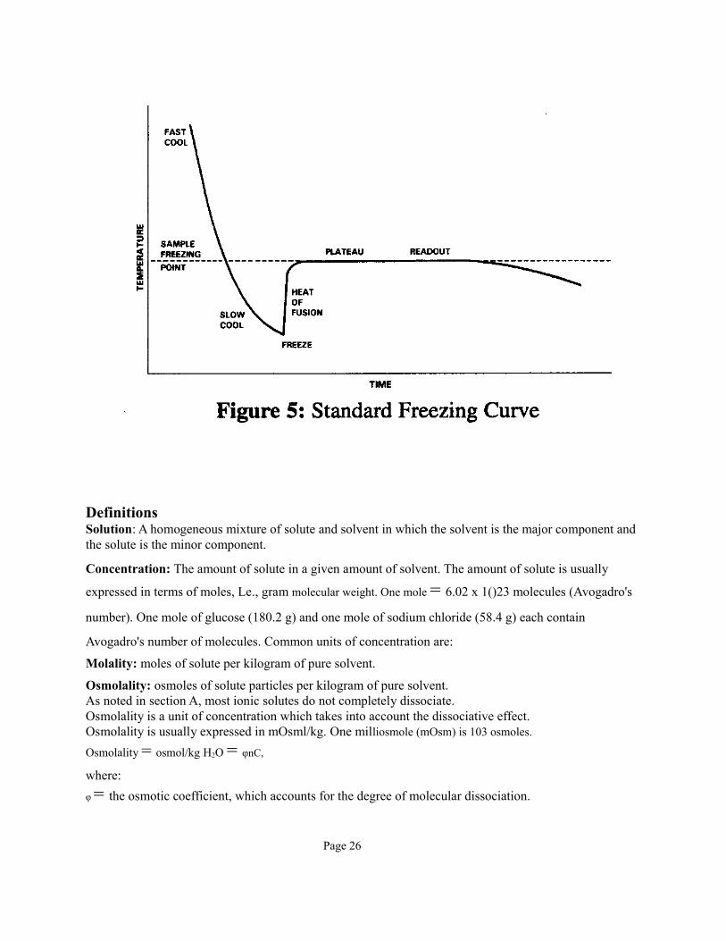
The quickest and most precise way to measure the freezing point of a solution is to supercool it several degrees below its freezing point and then mechanically induce the sample to freeze. The heat of fusion suddenly liberated causes the sample temperature to rise toward a temporary plateau wherein a liquid/solid equilibrium is maintained. The equilibrium temperature is, by definition, the freezing point of the solution.

The time over which liquid/solid equilibrium develops and is maintained is a function of the temperature differential between the sample and its environment and the ability of the surrounding materials to conduct heat. The cooling of the sample should be rapid, but not so fast that supercooling is uncontrolled. If the sample container and/or probe are allowed to become much colder (or much warmer) than the sample during the plateau, heat flow will distort the freezing curve.Sensitive thermistor probes monitor the sample temperature, control the degree of supercooling and freeze induction, and measure the freezing point of the sample. Automatic probe centering minimizes gradients and ensures uniform, precise sample temperature measurement. Fully auto-matic operation minimizes imprecision due to operator technique.

Figure 5 illustrates the temperature of a sample as it progresses through the freezing cycle and shows the action of the instrument at each stage.

Page 25

DefinitionsSolution: A homogeneous mixture of solute and solvent in which the solvent is the major component and the solute is the minor component.

Concentration: The amount of solute in a given amount of solvent. The amount of solute is usually

expressed in terms of moles, Le., gram molecular weight. One mole = 6.02 x 1()23 molecules (Avogadro's

number). One mole of glucose (180.2 g) and one mole of sodium chloride (58.4 g) each contain

Avogadro's number of molecules. Common units of concentration are:

Molality: moles of solute per kilogram of pure solvent.

Osmolality: osmoles of solute particles per kilogram of pure solvent.As noted in section A, most ionic solutes do not completely dissociate. Osmolality is a unit of concentration which takes into account the dissociative effect.Osmolality is usually expressed in mOsml/kg. One milliosmole (mOsm) is 103 osmoles.

Osmolality = osmol/kg H2O = φnC,

where:

φ = the osmotic coefficient, which accounts for the degree of molecular dissociation.

Page 26

n = the number of particles into which a molecule can dissociate.

C = the molal concentration of the solution.

Molarity: moles of solute per liter of solution.

Osmolarity: osmoles of solute particles per liter of solution.Although molarity and osmolarity are common units of measurement in other branches of chemistry, they are not used in osmometry because they are temperature dependent (water changes volume as the temperature varies) while molality and osmolality are not. However, in the case of simple, fairly dilute solutions, it is possible to convert between units if necessary.

Freezing PointlMelting Point. The temperature at which the liquid and crystalline phases of a substance will remain together in equilibrium.

Freezing Point Depression. When a solute is added to a solvent, the freezing point of the solvent is lowered. In aqueous solutions, one milliosmole of solute per kilogram of water depresses the freezing point by1.86 millidegrees Celsius (m°C).

Supercooling. The tendency of a substance to remain in the liquid state when cooled below its freezing point.

Crystallization Temperature. Aqueous solutions can be induced to freeze (i.e., crystallize) most reliably when supercooled. When supercooled, crystal formation is induced by agitating the solution (freeze pulse). The crystallization temperature is the temperature at which crystallization is induced. During crystalization, the heat of fusion raises the temperature of the sample to an ice/water freezing-point plateau.

Heat of Fusion. The heat released when the mobile molecules of a liquid are frozen into rigid crystals.

Freezing-Point Plateau. The constant temperature maintained during the time that ice and liquid exist in equilibrium after crystallization is initiated.

Measurement Procedure:

Equipment required:

• Sampler• Disposable Sample Tip• Chamber cleaner

1. Snap a sample tip into place on the sampler. The sample cell must be straight and firmly seated. Be careful not to crack the sample tip. Use rubber gloves to avoid contamination by perspiration on you finger tips.

2. Depress the sampler’s plunger and insert the sample tip at least ¼ inch below the surface of the fluid to be tested. Gently release the plunger to load a 20-μL sample.

Page 27

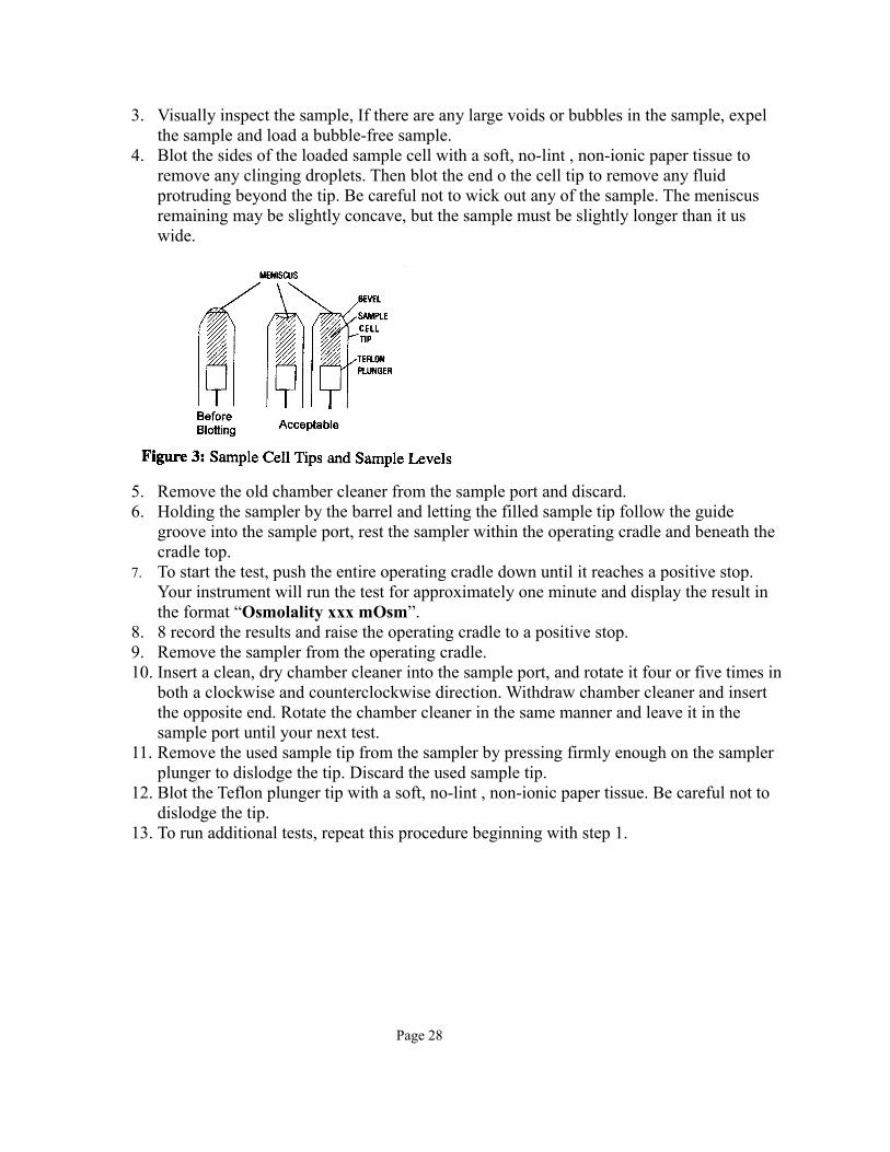
3. Visually inspect the sample, If there are any large voids or bubbles in the sample, expel the sample and load a bubble-free sample.

4. Blot the sides of the loaded sample cell with a soft, no-lint , non-ionic paper tissue to remove any clinging droplets. Then blot the end o the cell tip to remove any fluid protruding beyond the tip. Be careful not to wick out any of the sample. The meniscus remaining may be slightly concave, but the sample must be slightly longer than it us wide.

5. Remove the old chamber cleaner from the sample port and discard.6. Holding the sampler by the barrel and letting the filled sample tip follow the guide

groove into the sample port, rest the sampler within the operating cradle and beneath the cradle top.

7. To start the test, push the entire operating cradle down until it reaches a positive stop. Your instrument will run the test for approximately one minute and display the result in the format “Osmolality xxx mOsm”.

8. 8 record the results and raise the operating cradle to a positive stop.9. Remove the sampler from the operating cradle.10. Insert a clean, dry chamber cleaner into the sample port, and rotate it four or five times in

both a clockwise and counterclockwise direction. Withdraw chamber cleaner and insert the opposite end. Rotate the chamber cleaner in the same manner and leave it in the sample port until your next test.

11. Remove the used sample tip from the sampler by pressing firmly enough on the sampler plunger to dislodge the tip. Discard the used sample tip.

12. Blot the Teflon plunger tip with a soft, no-lint , non-ionic paper tissue. Be careful not to dislodge the tip.

13. To run additional tests, repeat this procedure beginning with step 1.

Page 28

ELR 4202CLABORATORY #4

Pressure Transducer Transient Response

Equipment:1. Computer with BioPac Pro Software2. MP100 with USB adapter and power supply. 3. TDS104A transducer4. Sphygmomanometer bulb and tubing with leur fitting added5. Leur stopcock to isolate sphygmomanometer bulb6. Tubing (size TBD) for catheter7. Leur Fitting appropriate for above tubing8. 60 mL syringe- modified with plunger removed and small leur adapter fitted in wall

about 15 to 20 % of the distance to the bottom of the tube.9. Leur tube fitting for pressure transducer.10. A Second leur stopcock to bleed and seal downstream end of pressure transducer.11. Syringe (1 mL) to introduce bubble near transducer. 12. Rubber glove, (expendable)13. Three fingered Test tube clamp14. Ring stand (any size that is convenient)15. Creeper clamp to fit outside of 60 mL syringe body.16. Scissors to cut disks from glove.17. Exacto knife or scalpel.18. Cigarette lighters

Prepare 100 mL deoxygenated water (100 mL) by boiling 250 mL of H2O on a heating plate for at least 10 minutes. When the boiled water is cooled, you may fill a syringe with 60 ml by aspiration. Do not pour or stir or otherwise mix the water with air. Alternately, you may use vacuum pump to pump down on a vacuum flask of water having a rubber stopper in the top. Have the flask on a stir plate and stir vigorously with a stir bar. Mild heating is also useful but not required if you do this.

Refer to pp 30 to 35 and 302 to 305 of Webster, 3

3 Medical Instrumentation: Application and Design, 3rd Edition, John G. Webster (Editor)ISBN: 0-471-15368-0 Hardcover 720 pages August 1997

Page 29

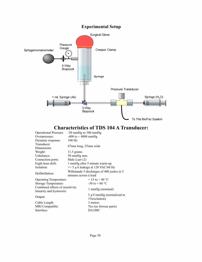
Experimental Setup

Characteristics of TDS 104 A Transducer:Operational Pressure: -50 mmHg to 300 mmHgOverpressure: -400 to + 4000 mmHgDynamic response: 100 HzTransducer Dimensions:

67mm long, 25mm wide

Weight: 11.5 gramsUnbalance: 50 mmHg maxConnection ports: Male Luer (2)Eight hour drift: 1 mmHg after 5 minute warm-upIsolation: <= 5 µA leakage at 120 VAC/60 Hz

Defibrillation:Withstands 5 discharges of 400 joules in 5 minutes across á load

Operating Temperature: + 15 to + 40 °CStorage Temperature: -30 to + 60 °CCombined effects of sensitivity linearity and hysteresis:

1 mmHg (nominal)

Output:5 µV/mmHg (normalized to 1Vexcitation)

Cable Length: 3 metersMRI Compatible: Yes (no ferrous parts)Interface: DA100C

Page 30

Procedure:Calibration:

1. Cut a disk of rubber from the glove large enough to fit over the end of the syringe with about ½ inch overlap

2. Stretch the rubber disk over the end of the syringe and fix it in place with the creeper clamp.

3. Apply pressure to the chamber at the top of the test tube until it reaches about 140 mm Hg.

4. Record the reading from the pressure transducer.5. Release the air from the test tube until the pressure reading is zero.6. Record the reading from the pressure transducer.

Exercise:

7. Cut a disk of rubber from the glove large enough to fit over the end of the syringe with about ½ inch overlap

8. Stretch the rubber disk over the end of the syringe and fix it in place with the creeper clamp.

9. Apply pressure to the air in the top of the test tube until it reaches about 140 mm Hg.10. Light the match11. Start recording of data with the Biopac system at once.12. Wait two seconds and use the match to pop the balloon.13. Wait one second and stop recording.

Replace the rubber disk and repeat the experiment to complete the following matrix

Sampling Rate

Pressure Transducer

Natural Frequency ω

Damping Ratio ζ

1 K Hz Without bubble50 Hz Without bubble1 K Hz With bubble*50 Hz With bubble*

. * Add a 200 µL bubble to the transducer through the three way stopcock closest to the transducer.

Data Analysis:

1. What is the initial value of the pressure, Pi? 2. What is the final value of the pressure, Pf?3. Calculate the damping ratio, ζ, of the pressure transducer four all four experimental

conditions. 4. Calculate the natural frequency of the experimental setup, ωn for all four experimental

conditions.

Page 31

5. Explain the discrepancies between the calculated values among all experimental conditions. Keep in the mind the difference between changing system parameters versus changing data collection parameters.

Page 32