Portland State University Portland State University

PDXScholar PDXScholar

Dissertations and Theses Dissertations and Theses

Spring 5-19-2015

Effects of Selective Logging and Roads on Instream Effects of Selective Logging and Roads on Instream

Fine Sediments and Macroinvertebrate Fine Sediments and Macroinvertebrate

Assemblages in the Clackamas Basin, Oregon Assemblages in the Clackamas Basin, Oregon

Paula Elizabeth Hood Portland State University

Follow this and additional works at: https://pdxscholar.library.pdx.edu/open_access_etds

Part of the Environmental Sciences Commons, and the Forest Management Commons

Let us know how access to this document benefits you.

Recommended Citation Recommended Citation Hood, Paula Elizabeth, "Effects of Selective Logging and Roads on Instream Fine Sediments and Macroinvertebrate Assemblages in the Clackamas Basin, Oregon" (2015). Dissertations and Theses. Paper 2407. https://doi.org/10.15760/etd.2404

This Thesis is brought to you for free and open access. It has been accepted for inclusion in Dissertations and Theses by an authorized administrator of PDXScholar. For more information, please contact pdxscholar@pdx.edu.

 

 

Effects of Selective Logging and Roads on Instream Fine Sediments and

Macroinvertebrate Assemblages in the Clackamas Basin, Oregon

by

Paula Elizabeth Hood

A thesis submitted in partial fulfillment of the requirements for the degree of

Master of Science in

Environmental Science and Management

Thesis Committee: Yangdong Pan, Chair

Eugene Foster Joseph Maser

Portland State University 2015

i  

 

Abstract

Logging and associated skid trails, haul routes, and roads can have significant

impacts on the magnitude and timing of sediments in streams in forested watersheds.

Loss of vegetation, soil compaction, use of heavy logging equipment, and alteration of

natural hydrologic patterns within the watershed can increase landslide rates, create

erosion, and generate fine sediments. Selective logging, also called thinning, is a logging

practice that leaves some trees within sale units unharvested. The ecological impacts of

thinning on stream ecosystems are not fully understood and need further study. My

hypothesis was that macroinvertebrate assemblages would be different in streams in non-

reference areas that contain recent selective logging compared to streams in reference

areas, and in downstream vs. upstream of selective logging units. I also hypothesized that

selective logging and high road densities would be associated with increased instream

fine sediments. I sampled water quality parameters and macroinvertebrates in three

managed and three reference streams in the Clackamas River Basin during the field

season of 2013. Turbidity, temperature, dissolved oxygen, conductivity, total dissolved

solids (TDS), suspended sediment concentrations (SSC), and flow were sampled at each

stream on four occasions during spring through early fall. Macroinvertebrates were

sampled once in late summer or early fall. EPA rapid habitat assessments, canopy cover,

pebble counts, embeddedness, and slope were also determined. Water quality parameters

and macroinvertebrate indices in reference and non-reference sites were compared using

t-tests, Welch’s tests, or rank based equivalents. Macroinvertebrate assemblage patterns

ii  

 

and associated environmental variables were characterized using non-metric

multidimensional scaling (NMDS) ordination plots and envfit overlays.

Macroinvertebrates had higher abundance and taxa richness in non-reference streams,

and indices suggested poorer water quality in non-reference streams. Non-reference

streams had a lower percentage of shredders and a higher portion of gatherer-collectors.

Associations between land use, fine sediments, and changes in macroinvertebrate metrics

and community assemblages were apparent at the reference vs. non-reference scale. It is

likely that macroinvertebrates are responding, at least in part, to past logging and high

road densities in non-reference streams. Fewer indications were found that recent logging

may be affecting water quality and macroinvertebrates. Pearson’s correlation coefficients

show that the percent of recent logging upstream of study sites was correlated with

several measures of fine sediments, suggesting that recent land use may be affecting

sediment levels at the subwatershed scale. Stream temperatures increased from upstream

to downstream in non-reference sites. Though no continual stream temperature data were

collected in this study, the history of continuing temperature standard exceedances in the

area suggest that further investigation of how selective logging may be affecting stream

temperature and other water quality parameters in the Clackamas Basin is warranted. No

other differences in water quality parameters were found from upstream to downstream,

possibly because water quality was sufficiently protected, or because signals from land

use impacts may be obscured by a several factors, including upstream confounding

factors such as roads and past logging, and natural variability.

iii  

 

Dedication

This thesis research is dedicated to my daughter, Wren Velasco-Overson, who is

my truest inspiration to do the best that I possibly can in all things. Wren has been

continually good humored about sharing her childhood with my endless academic work.

In addition, she kept complaints to a minimum when getting stuck carrying other peoples’

gear many miles in the woods on more than one occasion.

iv  

 

Acknowledgements

I would like to extend my sincere and lasting gratitude to my graduate advisor,

Dr. Yangdong Pan, who has always been generous with his insights, wisdom, and

patience. I benefited greatly from his scientific expertise and thoughtful approach to

teaching, and from his faith in the learning process. I would also like to thank my

committee members, Dr. Eugene Foster and Dr. Joseph Maser, for their help and support.

I am lucky to have had such talented and gracious guides help me through my graduate

school journey.

My family provided unending patience and help of all kinds throughout my

graduate studies. I could not have done this work without the support of my mother,

Carolina Hood, and my sweetheart, David Kennedy.

Many people volunteered their time and support to help with my thesis research. I

am humbled by the selflessness of the many people who dedicated countless hours to this

project. Special thanks to Amy Balint, David Kennedy, Michael Krochta, and Monica

Mogileswky, who all went far above the call of volunteer duty and spent days and even

weeks doing field work in often cold and wet conditions. I owe a special debt of gratitude

to Monica for having more motivation at times than I did for hiking many miles day after

day in the pouring rain, and for maintaining a more positive attitude than any of us. You

are perhaps the toughest trooper of all. Erin Poor and Naomi Lowinger did a lion’s share

of laboratory work, and provided many hours of great conversation during endless debris

sorting. Other wonderful volunteers that I wish to thank include: Autumn Rainha,

v  

 

Brendan Phoenix, Danielle Fagan, David Roth, Jess Dalesky, Jim Destabler, Jonathan

Hartigan, Gambit McKay, Karen Coulter, Kecia Jones, Lola Goldberg, Maksim Zemtsov,

Matthew Przyborski, Maysa Miller, Michael DuCharme, Michael Miller, Michael

Newman, Nathan Weick, Rick Park, Stephanie Moe, and Thomas DeAlameda. I

apologize if I have inadvertently left anyone off of this list. It was my sincere honor to

spend many hours investigating forested streams and the macroinvertebrates that live

there with all of you.

vi  

 

Table of Contents

Abstract................................................................................................................................ i

Dedication...........................................................................................................................iii

Acknowledgements........................................................................................................... .iv

List of Tables ....................................................................................................................vii

List of Figures.................................................................................................................. viii

Chapter 1 Introduction.........................................................................................................1

Chapter 2 Methods……….................................................................................................19

Chapter 3 Results...............................................................................................................44

Chapter 4 Discussion.........................................................................................................71

References………............................................................................................................100

vii  

 

List of Tables

Table 1: Family Biotic Index score water quality ranking…….……...………...……….41 Table 2: Summary of significance tests for water quality and environmental variables...45

Table 3: Summary of all water quality and environmental parameters…………….....…48 Table 4: Mean, median, and range of values for selected variables……………..………51

Table 5: Selected macroinvertebrate metrics in non-reference and reference streams..…56 Table 6: Dominant taxa………….……………………………………………...…….….57

Table 7: NMDS 1 and NMDS 2 scores for significant macroinvertebrates…....………..62 Table 8: NMDS 1 and NMDS 2 scores for significant environmental variables…….….69

viii  

 

List of Figures

Figure 1: Conceptual model of sediment generation and transport……..………………..4 Figure 2: General area, land use, and ownership of the Clackamas Basin, Oregon……..20

Figure 3: General location of sample sites ……………………………...……………….31 Figure 4: Generalized depiction of upstream/downstream study design …………..……33

Figure 5: Boxplots of average turbidity in all streams….……………..…………………45 Figure 6: Boxplots of turbidity, total dissolved solids, temperature………..……………46

Figure 7: Boxplots of embeddedness, pebble counts, canopy cover, and EPA scores…..47 Figure 8: Boxplots of selected macroinvertebrate metrics……………….…...…………55

Figure 9: Boxplots of macroinvertebrate functional feeding groups.....…………………59 Figure 10: Dominant taxa on the NMDS ordination plot.……………………………….61

Figure 11: Bubble plots of dominant taxa……………………...………………………...63 Figure 12: Bubble plots showing abundance and richness………………………………64

Figure 13: Bubble plots showing gatherer-collectors and shredders……………. ……...64 Figure 14: Envfit of significant environmental variables on the NMDS plot.…...………66

Figure 15: Envfit of all environmental variables on the NMDS plot……...……...…..…67 Figure 16: Pearson’s correlation coefficients for selected variables…………………….70

Figure 17: Roads and past logging in the Fish Creek Divide circa1994………………...91

1  

 

Chapter 1: Introduction

Logging, roads, and fine sediment delivery:

Timber harvest and associated skid trails, haul routes, and roads can have

significant impacts on the magnitude and timing of sediment loading into streams in

forested watersheds (Croke and Hairsine 2006, Lewis et al. 2001, Wood and Armitage

1997). Loss of vegetation, soil compaction, and alteration of natural hydrologic patterns

within the watershed can create erosion, increase landslide rates, and generate fine

sediments, some of which may ultimately be delivered into stream channels (Guthrie

2001, Harr and Coffin 1992, Hicks et al. 1991, Jones 2000, Jones and Grant 1996, Lewis

et al. 2001, Montgomery et al. 2000, Wemple et al. 2000). For example, Montgomery et

al. (2000) found that shallow landslide rates (i.e., landslides within the weathered bedrock

portion of surface) increased in logged areas in the Oregon Coast Range by three to nine

times that of background conditions. In the Fish Creek Watershed located in the

Clackamas basin, Oregon, the Forest Service’s Watershed Analysis found that landslide

rates associated with roads and/or harvest areas were three times more common in survey

areas over a 43 year study period compared to background levels (USFS 1994). Wemple

et al. (2000) found that road-related erosion and landslide features generated 13,000 cubic

meters of sediment in two small forested watersheds in the western Oregon Cascades

along 230 kilometers of road during one 100-year storm event. Lewis et al. (2001) found

that sediment loads increased over 100% in small tributaries after logging. Alteration of

natural sediment regimes leading to sediment related imbalances are a major cause of

2  

 

stream impairment listings, affecting approximately 40% of US river miles (Nietch et al.

2005, USEPA 2006).

The regulation of instream sediment pollution continues to be controversial. For

example, in 2010, the 9th Circuit Court of Appeals ruled that sediment inputs from roads

could be considered a point source of pollution (Northwest Environmental Defense

Center v. Brown, 2010). This ruling was overturned in 2013 (Decker v. Northwest

Environmental Defense Center, 568 U.S., 2013), and sediment inputs from roads and

timber practices were again considered to be non-point pollution. Stream sediment

pollution in relation to forestry practices is controlled through best management practices,

a set of mitigation guidelines designed to support compliance with the Clean Water Act

through lessening erosion, soil compaction, and other potential sediment sources related

to logging and roads (USFS 2012). Environmental laws such as the Clean Water Act and

the Endangered Species Act mandate management of water bodies in order to protect

beneficial uses, water quality standards, and critical habitats. However, due to the natural

variation of instream sediment loading, as well as the complexities and expense

associated with estimating or quantifying stream sediments, clear guidelines for

determining reference or recommended sediment levels have not been established

(USEPA 2006). In addition, without sufficient baseline data, determining guidelines and

criteria for sediment levels, or performing effective and meaningful monitoring in

relation to current land management activities, is difficult at best. Currently, there is a

lack of unified sediment criteria across states, with many states having vague, qualitative,

or non-existent guidelines for sediment loading. Unfortunately, there is little scientific or

3  

 

agency consensus on what constitutes background sediment levels or what guidelines are

needed to protect biota in differing aquatic environments (USEPA 2006).

While it is difficult to quantify natural background sediment levels in streams,

studies suggest that logging and associated roads alter watershed hydrology and sediment

levels in comparison to non-disturbance conditions or controls. For example, changes in

historic watershed hydrologic regimes and processes due to logging and associated roads

can alter the timing and magnitude of stormwater runoff into streams, which in turn may

affect sediment delivery regimes (Croke and Hairsine 2006, Wemple et al. 2000). Excess

fine sediments generated by road related erosion or harvest related soil compaction may

be carried farther across the landscape because of decreases in water infiltration or runoff

rates over damaged soils, which in turn can cause an increase in the distance of overland

flow transporting the sediments (Figure 1). Thus, the sediments generated by

management activity may be more likely to reach streams (Croke and Hairsine 2006,

Nietch et al. 2005, Wemple et al. 2000). Areas of greatest soil compaction are skid trails

and log haul routes, which are often responsible for the largest increases in overland

flows and peak flows (Nietch et al. 2005, Jones and Grant 1996). In addition, improper

road drainage can cause gullies, landslides, and other erosional features, which in turn

lead to sediment generation, increased runoff, and more direct and rapid transport of

runoff and sediment to streams (Croke and Hairsine 2006, Wemple et al. 2000).

Furthermore, the distance of travel required for sediments to enter streams may be

shortened by the artificial extension of stream networks by roads and culverts (Croke and

Hairsine 2006, Wemple et al. 1996). Increases in the efficiency of delivery of water and

4  

 

sediment to streams due to road networks and changes to soil infiltration and

groundwater inputs can affect the timing, magnitude, duration, and frequency of sediment

inputs.

Figure 1: Conceptual model of sediment generation and transport, adapted from Fredrisksen (1982).

In addition to altering overland flow and sediment creation and transport

processes, harvest management activities can alter base and peak flows regimes and

hydrograph shape (Harr and Coffin 1992, Jones and Grant 1996, Jones 2000, Lewis et al.

2001, Wemple et al. 1996). Altered flow regimes can potentially affect instream sediment

5  

 

dynamics by causing sediments to scour out or embed stream substrates (Croke and

Hairsine 2006, Lewis et al. 2001, Moore and Wondzell 2005, USEPA 2006). Harr and

Coffin (1992) found that both clear-cutting and thinning increased the amount of snow

pack, rates of snowmelt, leading to increases in both magnitude and timing of peak flows.

Lewis et al. (2001) found that clearcutting increased storm runoff by approximately 58%,

and partial cutting of 30 to 50% increased runoff by approximately 23% in the Caspar

Creek Experimental Forest in the northern California coastal range. In addition, roads

increase peak flows by intercepting surface and subsurface flow, and diverting it into

culverts and ditches that drain into streams (Wemple et al. 1996). Instream sediment

dynamics such as timing and placement of fine sediment deposition, embeddedness, and

scour are affected by stream power and flow regimes (Moore and Wondzell 2005, Wood

and Armitage 1997). Sediment imbalances can include sediment starvation, streambed

scour, and embeddedness. Embeddedness refers to the degree to which coarser stream

substrates are covered or surrounded by fine sediments (USEPA 2006). Changes in

watershed hydrology after logging were found to be significant causes of increased

stream sediment loading (Troendle and Olsen 1993, Lewis et al. 2001). Alteration of peak

flows may increase flooding and also cause damage to culverts and bridges (Moore &

Wondzell 2005), further increasing erosion and fine sediment inputs.

Logging and instream habitats and fauna:

Fish, amphibians, and macroinvertebrate communities may be negatively

impacted by excess fine sediment inputs resulting from logging and roads (Bryce et al.

2010, Nietch et al. 2005). Increases in fine sediment loading can cause simplification of

6  

 

complex habitats and channel structure either through settling on or scouring out the

streambed (Cover et al. 2008, Nietch et al. 2005). As a result, habitats such as pools,

riffles, and side channels required by stream organisms for egg laying, resting, hiding,

and rearing of young may be degraded or eliminated (Bryce et al. 2010, USEPA 2006). In

addition, excess fine sediment loading, particularly in combination with the alteration of

flow regimes and hydrologic processes, may negatively impact stream channel stability,

limit hyporheic exchange, and alter groundwater inputs, potentially degrading conditions

for stream organisms by further increasing sediment loading, decreasing necessary

physical habitat, and altering stream water volume which can affect temperature and

dissolved oxygen, and limit resources (Croke and Hairsine 2006, Moore and Wondzell

2005, Nietch et al. 2005, USEPA 2006). Fine sediment inputs exceeding natural

background levels may bury and smother fish and amphibian eggs or young, decrease

dissolved oxygen (DO) levels, interfere with behaviors such as mating, feeding and

predator avoidance, cause shifts in macroinvertebrate community structures, and increase

macroinvertebrate drift rates (Bryce et al. 2010, Nietch et al. 2005, USEPA 2006). For

example, Coho salmon egg survival and fry emergence were negatively correlated with

embedded fines of greater than 10%. In addition, when fines exceeded 20%, average

survival decreases dramatically (Cederholm 1980). Macroinvertebrate drift rates

increased significantly when exposed to suspended sediment concentrations of 8 mg/L

for 5 hours, though ephemeroptera and plecoptera drift more rapidly upon exposure to

sediments compared to those not exposed to sediments. Some ephemeroptera species,

when exposed to concentrations of suspended sediments greater than 29mg/L for 30 days,

7  

 

will disappear entirely. Longer exposure durations and smaller particle sizes caused

increased rates of drift (IDEQ 2003).

Quantifying sediment loading in small watersheds: methods and limitations

Long term sediment loading and hydrograph information for small forested

watersheds are often lacking, creating difficulties in determining historic, as well as

current, sediment levels (USEPA 2006, USGS accessed 2012). In addition, gaps remain

in our understanding of the sediment delivery processes from disturbed sites to streams.

Consequently, the effects associated with timber harvest on stream sediment loading are

difficult to quantify or predict (Croke and Hairsine 2006). Few lower order streams are

gaged or monitored in the long term, resulting in a scarcity of statistically meaningful

streamflow, hydrograph, or biological data for small watersheds (Tague and Grant 2004,

USEPA 2007). Detailed or continuous measurement of streamflow and sediment loading

without established gages is difficult and costly, limiting the ability of scientists to

perform detailed long term studies on these parameters in relation to land management

impacts. Furthermore, methods used to measure instream sediments have a variety of

shortcomings or associated challenges such as expense, physical impracticality, and

subjectiveness.

Methods used to measure bedded sediments, such as percent of fines by volume

and/or area can be impractical to measure in wadeable mountain streams where obtaining

stream substrate cores may be difficult and expensive due to large cobbles and boulders

and rapid streamflow. Methods such as Wolman pebble counts, substrate stability,

residual pool volumes, pool frequency and depth, professional judgment, and pictures can

8  

 

be difficult to quantify precisely, may not accurately reflect the amount of bedded

sediments, may be subjective, or may not be appropriate for looking at recent impacts

(Bauer and Ralph 2001, Olsen et al. 2005, Whitman et al. 2003). Other methods include

basket, tray, and pit samplers. These are considered fairly accurate by the USGS, though

they can be time consuming and costly for smaller agencies or individual scientists. The

USGS is in the process of developing other methods to measure bedded sediments, such

as radar and sonar based technologies, but these methods have yet to be finalized and

vetted, and are not yet widespread (Gray et al. 2010).

Due to the expense and time associated with gathering bedded sediment data,

methods for measuring suspended sediments, such as turbidity and/or total suspended

solids (TSS), are more frequently used by scientists and agencies (Gray et al. 2010). Most

US states base sediment criteria on measures of turbidity and/or total suspended solids

(USEPA 2006). Turbidity is most commonly used as a surrogate for sediment loading,

due to ease of measurement, generation of precise and quantifiable data, and relative low

cost. However, examining multiple metrics is recommended (USEPA 2006). Turbidity is

the measure of the cloudiness of the water, as estimated by how effectively a beam of

light passes through water, and is generally measured in units of Nephelometric Turbidity

Units (NTUs) or, less frequently, Formazin Turbidity Units (FTUs) (Henley et al. 2000,

USEPA 2006, Rasmussen et al. 2011). Suspended sediment particles interfere with light

transmittance and cause an increase in cloudiness, and so turbidity is correlated with

suspended sediment in the water column (USEPA 2006, Rasmussen et al. 2011).

Measurements are made through discretely captured field samples, by streamgage

9  

 

sensors, or by instream turbidity sensors that can feed into data logger software.

However, a key drawback of using turbidity as a surrogate for sediment loading is that

the majority of sediments are transported in the stream water column during storm events,

and patterns of transport during storm events are erratic (Edwards and Glysson 1999). For

example, peak sediment transports may be present directly before or after peak flows, and

do not exhibit reliable temporal patterns (Ellison et al. 2010). In other words, measuring

turbidity at a particular moment or season may not accurately represent the actual

sediment load of the stream, and may fail to detect high sediment pulses or deviation

from natural timing or frequency. Discrete field sampling or even instream turbidity

sensors may miss major sediment movement events in the stream (Ulrich 2002). In

addition, the degree to which turbidity and suspended sediments are correlated is

controversial. The size, shape, and mineral content of the particles, as well as the water

color and temperature, can affect turbidity readings. Also, the instrumentation for

measuring turbidity is not standardized, and can further contribute to variability in

readings (Packman et al. 2000). For example, different models of turbidity meters may

have 2 to 4 receptors for light sensing, and therefore have different levels or patterns of

accuracy (Anderson 2005). Henley et al. (2000) claims that using turbidity as a surrogate

for sediment is dubious, and recommends that turbidity at least be calibrated to suspended

sediment concentrations for greater accuracy (Henley et al. 2000). The USGS

recommends using turbidity data which has been calibrated to suspended sediment

concentrations to create a suspended sediment load curve to increase accuracy and

prediction (Rasmussen et al. 2011). On the other hand, Packman et al. (2000) found a

10  

 

very high correlation (R2 of 0.96) between turbidity and TSS when examining 9 streams

in both urban and forested watersheds. They suggest that turbidity is an adequate and

probably viable measure of TSS (Packman et al. 2000), and so strengthens the case for

using turbidity as a surrogate for sediment loading. Rasmussen et al. (2011) report that

TSS measurements tend to be biased low and that SSC is a preferable method of

estimating suspended sediments. They also found that SSC has a strong linear correlation

to turbidity, and that when the correlation is proportional, turbidity can be used to

estimate SSC values (Rasmussen et al. 2011), though data may need to be log

transformed in order to display a linear relationship (Ellison et al. 2005, Galloway et al.

2005). The USGS recommends using SSC over TSS, as TSS measurements tend to be

biased low 25 to 34 percent, and SSC methodology is more standardized and accurate

(USGS 2000). Increasingly, the USFS and the USGS use continuous instream turbidity

sensors which, when a specified turbidity is exceeded, trigger a pump sampler to obtain a

limited number of water samples to be analyzed later for suspended sediment

concentrations (Gray et al. 2000, Lewis 2003).

Macroinvertebrates, fish, periphyton, and mussels are used by scientist and

agencies as bioindicators of stream health, and one or more is generally measured in

conjunction with direct estimates of suspended and/or bedded sediments (USEPA 2006).

Natural variability of sediment loading across watersheds is high (Tague and Grant 2004,

USEPA 2006), and ecological responses to sediment levels may be complex (Herlithy et

al. 2005, Reid et al. 2010, Smith et al. 2009). These factors, combined with the challenges

of directly measuring fine sediments, necessitate quantifying of one or more biological

11  

 

indicators in order to obtain a more robust picture of overall ecosystem health. While

sediment pulses, even those that are frequent, may not reliably coincide with the timing

of turbidity samples, they nevertheless may affect stream organisms. Measures of

biological indices have been shown to be effective in detecting ecosystem impacts in

logged watersheds in relation to sediment stress as well as other variables. In their study

comparing logged and reference watersheds in the Ouachita Mountains of Arkansas,

Hlass et al. (1998) found that in logged watersheds, turbidity and TSS showed inverse

correlations with scores from a Modified version of the index for biotic integrity (IBI), an

index which takes into account multiple biological metrics. In Georgia, low IBI scores

based on fish were correlated with TSS values greater than 8 mg/L in low flow stream

conditions. Streams with TSS values of less than 6 mg/L had high IBI scores (IDEQ

2003).

Macroinvertebrates are often selected as bio-indicators because they are

ubiquitous in all stream orders (including those outside of the range of fish and mussels),

easy to collect, and relatively simple to identify to necessary taxonomic category. In

addition, some macroinvertebrate feeding groups, families, and/or genera are more

sensitive to excesses of fine sediments then others, and so have relatively predictable

shifts in community structure or composition when sediment stress is present

(Miserendino and Masi 2010). For example, Miserendino and Masi (2010) found that

higher abundance of the collector-gatherers correlated with fine sediments in areas where

riparian logging had disturbed stream channels. Kreutzweiser et al. (2005) also found

significant increases in gatherer taxa which seemed to be correlated to a significant

12  

 

increase in fine sediments in some logged areas. Reid et al. (2010) found that logged

areas showed increases in Diptera, mollusks, worms, and a decrease in Ephemeroptera,

and concurrently showed increased fine sediments, temperature, and algal mass. Wood

and Armitage (1997) also found that sediment rich environments favored oligochaetes

and chrinomids. In addition, they found that particular species of ephemeroptera were

better adapted to high sediment and low oxygen environments than others. They also

found that filter feeders may be negatively affected, as their feeding apparatuses may

become clogged by fine sediments, and that increases in turbidity may limit the amount

of light reaching the stream substrate, thus limiting algae production and affecting the

entire food web (Wood and Armitage 1997). However, biological responses to

disturbances such as logging can be complex and variable. Studies have shown seemingly

conflicting responses in the macroinvertebrate community following logging. For

example, macroinvertebrate densities, abundance, diversity, and species richness have

been found to decrease, increase, or remain the same following logging in different

studies. This may be due, at least in part, to heterogeneity in geomorphology, size of and

response to riparian buffers, utilization of different indices with differing levels of

sensitivity, upstream watershed characteristics, stage of forest and macroinvertebrate

recovery, seasonal variability, and scale (Herlithy et al. 2005, Reid et al. 2010, Smith et

al. 2009). Increasingly, current studies are elucidating the nuances associated with

macroinvertebrate responses to disturbance, and a greater understanding of these

responses will continue to increase the accuracy and strength of their use as a bioindicator

of stream health in relation to logging and associated sediment inputs.

13  

 

A variety of indices for macroinvertebrate analysis include: taxa richness, ratio or

relative abundance of scrappers to filterer and/or collector functional feeding groups,

ratio or relative abundance of shredder functional feeding group to total number, percent

contribution of dominant taxa, Shannon and Simpson diversity indices, Hilsenhoff Biotic

Index (HBI), Family Biotic Index, community similarity index, community loss index,

index of similarity between two samples, and the Pinkham and Pearson community

similarity index (Klemm et al. 1990, Barbour et al. 1999). Smith et al. (2009) looked at

total invertebrate abundance, taxon richness, rare taxon, and looked at whether functional

feeding groups were statistically similar between reference and disturbed sites (Smith et

al. 2009). The New Zealand Macroinvertebrate Working Group looked at abundance and

rare taxa (Stark et al. 2001). The fine sediment bioassessment index (FSBI) developed by

Relyea et al. (2000) identifies multiple benthic macroinvertebrates by species or taxa that

can be used as indicators of fine sediment levels based on their sediment tolerance. They

found EPT and Simpsons were not sensitive to varying sediment levels (Relyea et al.

2000). The FSBI was further investigated by Relyea et al. 2012 and was found to be

successful in indicating sediment impairment (Relyea et al. 2012).

Natural variability of fine sediment loading is influenced by numerous factors

including topography, channel morphology, gradient (USEPA 2006), land cover (Allan et

al. 2004), general rock type (Johnson et al. 2003), soil erodibility (USEPA 2006), road

density (Cederholm et al. 1980), stream order (Johnson et al. 2003), and catchment size

(Bolstad and Swank 2007). For example, the geology of an area plays a key role in

affecting fine sediment loading in streams (USEPA 2006), and is one of the main drivers

14  

 

of streamflow regimes (Tague and Grant 2004). Soft sedimentary rocks, considered

erosive, are more likely to generate sediment in relation to land management disturbances

than hard volcanic rocks, which are considered resistant (USEPA 2006). Similarly,

Dyrness (1967) reported that the pyroclastic rocks in the western Cascades such as tuffs

and breccias are more prone to soil mass movements than areas containing underlying

bedrock of basalt or andesite (Dyrness 1967). Swanson and Swanston (1977) also

reported that pyroclastic rock that has been extensively weathered is the most susceptible

to earthflow and creep, and that these features generate a large portion of instream

sediments. Complex patterns of creep and earthflows are formed over larger areas of slow

mass movement, and rates of movement may vary considerably among discrete creep or

movement areas. Movement is most likely to take place or become accelerated in times

of higher soil moisture conditions when precipitation or snowmelt is occurring (Swanson

and Swanston 1977).

Geology, soil porosity, and underlying bedrock permeability have pronounced

effects on water infiltration and runoff rates (Moore and Wondzell 2005). Tague and

Grant (2004) found that the different geologic rock formations of the western Cascades

vs. the high Cascades had such a pronounced effect on groundwater, subsurface flow, and

consequently streamflow, that they could be used as a reliable predictor of peak and base

flow responses (Tague and Grant 2004), which in turn can influence sediment dynamics

(Croke and Hairsine 2006, Moore and Wondzell 2005). The western Cascades are

characterized by shallow soils with high clay content, which can limit groundwater

storage capacity and cause rapid subsurface flows, making peak flows flashier and base

15  

 

flows lower (Tague and Grant 2004). The high Cascades, on the other hand, have blocky

lava rock formations with many crevices and fractures, allowing for deep and slower

subsurface flow and large aquifer storage capacity. As a consequence, high cascades base

flows are comparatively larger and colder, and peak flows less flashy. The authors also

pointed out that groundwater inputs may play an equally important role in base and peak

flows as snowmelt (Tague and Grant 2004). In the Western Cascades, rain-on-snow

events are the primary drivers of peak flows, and streamflows are usually highest in the

months from November to April (Harr and Coffin 1992).

Need for study

While numerous studies have investigated the effects of clearcut logging on

erosion, landslide rates, and fine sediment generation (Croke and Hairsine 2006, Guthrie

2001, Hicks et al. 1991, Jones 2000, Jones and Grant 1996, Lewis et al. 2001,

Montgomery et al. 2000, Troendle and Olsen 1993), fewer studies have examined how

selective harvest practices affect sediment dynamics and instream sediment loading

(Kreutzweiser and Capel 2001, Reid et al. 2010). Additional field studies are needed in

order to help determine both background instream sediment levels, and levels in response

to selective harvest practices in small forested watersheds. Additional field data would

also facilitate more accurate modeling of the effects of land management practices on

sediment loading, hydrograph shape, and other hydrologic processes (Croke and Hairsine

2006, USEPA 2006), as well as possible impacts on biota. In particular, more information

regarding instream sediment levels is needed in areas where multiple uses and/or legal

16  

 

mandates may cause conflicts between ecological resources such as endangered salmon

and current logging practices.

While selective logging is likely to be less environmentally destructive than

clearcut logging in most situations, the extent of its impacts on forest health and stream

water quality is not clear. Little research has been done on water quality in relation to

selective logging, and the research that exists has often yielded contradictory or

ambiguous results. Some studies found selective logging may be associated with

increases of instream fine sediments (Kreutzweiser et al. 2005, Miserendino and Masi

2010), changes in macroinvertebrate community structure or metrics (Flaspohler et al.

2002, Kreutzweiser et al. 2005), alterations in nutrient cycling and leaf litter

decomposition rates (Lecerf and Richardson 2010), and increases in stream temperatures

(Guenther et al. 2012). However, others have found little or no change in stream fine

sediment levels (Kreutzweiser and Capell 2001) or macroinvertebrate community

structures (Gravelle et al. 2009). Kreutzweiser et al. (2005) found only limited changes to

macroinvertebrate community structure that tend to accompany specific riparian

disturbances, such as roads or skid trails disturbing soils near streams. However,

Flaspohler et al. (2002) noted that changes to biota associated with selective logging were

found decades after logging. Given that selective logging is taking place on many

thousands of acres of public and private lands, a more clear and detailed understanding of

the possible effects associated with selective logging is necessary in order to protect

riparian and aquatic resources. Investigation of possible impacts at multiple scales in

diverse environmental and geologic conditions, cumulative impacts, and chronic, sub-

17  

 

lethal effects on biota may be necessary in order to develop a sufficient understanding of

how biotic and abiotic resources may be affected. Possible thresholds, complex temporal

responses, long-term effects, and integrated ecosystem interactions should be considered.

Purpose and hypotheses

The objective of this study is to determine the effects of selective logging

practices and associated roads on the magnitude of instream sediment loading in small

forested watersheds in the Clackamas Basin in Oregon. To this end, I focused on stream

turbidity as a surrogate for sediment loading (USEPA 2006) in first, second, and third

order streams in managed and unmanaged watersheds in the Clackamas. In addition, I

sampled macroinvertebrates, and measured stream conductivity, total dissolved solids,

suspended sediment concentrations, and substrate embeddedness and pebble counts. I

hypothesized that macroinvertebrate assemblages would be different in reference vs.

streams with adjacent selective logging units with recent logging (non-reference streams),

and in reaches downstream of selective logging units vs. upstream reaches. I also

hypothesized that selective logging and high road densities would be associated with

increased instream fine sediments. I expected macroinvertebrate taxa associated with fine

sediments in other studies to increase, while those found to be sensitive to fine sediments

are expected to decrease (Angradi 1999, Reylea et al. 2012).

Macroinvertebrate responses to disturbances can be variable and complex. As a

result, the expectations concerning possible macroinvertebrate patterns in relation to

logged and unlogged areas in this study encompass a number of possible outcomes.

Reylea et al. (2012) identified the sediment tolerance levels of approximately 100

18  

 

macroinvertebrate taxa. This suggests that perhaps taxa considered to be sediment

intolerant in other studies may show patterns of presence or absence in this study (Reylea

et al. 2012). Macroinvertebrate responses may also include non-sediment specific

responses to logging such as greater abundance of emergent insects in impacted areas

(Banks et al. 2007, Progar and Moldenke 2009). I expected macroinvertebrate community

structures and assemblages to show distinct patterns in relation to harvest and to

increasing road densities, though responses may vary according to degree, size, and age

of logging units. In reference areas and upstream of logging units, I expected shredders

and taxonomic groups that are intolerant of sediment to comprise a higher percentage of

overall macroinvertebrate samples (Herlithy et al. 2005, Reid et al. 2010, Smith et al.

2009). I expected to find a higher abundance of collector-gatherers in reference streams,

and downstream of logged areas (Miserendino and Masi 2010). I also expected that the

percent of dipterans and certain families of Ephemeroptera will increase (such as the

Baetidae) (Waters 1995), while Plecoptera and other Ephemeroptera taxonomic groups

will decrease (IDEQ 2003, Wood and Armitage 1997). Additionally, in watersheds with a

relatively small percent of logged area, I expected there to be an increase in overall

diversity and abundance of macroinvertebrates due to the combination of the opening of

the canopy from riparian selective logging and increased nutrient input combined with

overall good water quality from upstream inputs. Finally, I expected that

macroinvertebrate community composition will show patterns of dissimilarity between

reference and non-reference sites when plotted on ordination plots.

19  

 

Chapter 2: Methods

Clackamas River Basin Site Description

The Clackamas River Basin is located approximately 48 kilometers southeast of

Portland, Oregon (Figure 2). The Clackamas River is a tributary of the Willamette River.

It drains approximately 2,435 square kilometers, and ranges in elevation from near sea

level to just over 2,134 meters (Salminen 2005). From the headwaters at the Ollalie Lakes

area in Mt. Hood National Forest, to just above the North Fork reservoir, the Clackamas

River drains a watershed of approximately 1,725 square kilometers- this area

encompasses much of the portion managed by the Forest Service. The majority of the

lower Clackamas Basin is privately owned, while the upper Basin (which is more than

half of the entire basin) is publicly owned, most of which is managed by the Forest

Service. The major tributaries of the Clackamas River are the South Fork of the

Clackamas, Fish Creek, the Roaring River, the Oak Grove Fork of the Clackamas, and

the Collawash River. In 1988, a 76 kilometer stretch of the Clackamas was designated

Wild and Scenic by Congress. This 76 kilometer stretch begins in the Ollalie Lakes area

and ends at Big Cliff, just upstream of the North Fork Reservoir (USFS 1993).

20  

 

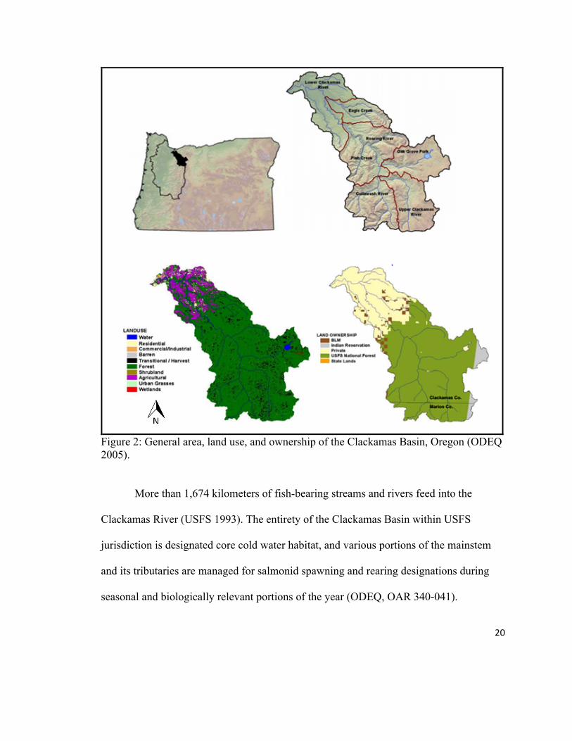
Figure 2: General area, land use, and ownership of the Clackamas Basin, Oregon (ODEQ 2005).

More than 1,674 kilometers of fish-bearing streams and rivers feed into the

Clackamas River (USFS 1993). The entirety of the Clackamas Basin within USFS

jurisdiction is designated core cold water habitat, and various portions of the mainstem

and its tributaries are managed for salmonid spawning and rearing designations during

seasonal and biologically relevant portions of the year (ODEQ, OAR 340-041).

 

21  

 

Spawning and core cold water designations are used in reference to temperature standards

for regulatory purposes (ODEQ, OAR 340-041; ODEQ, accessed 2015), and these

beneficial uses may be negatively affected by excess fine sediments (Bryce et al. 2010,

USEPA 2006).The Clackamas River Basin carries what is believed to be the last

significant and self-sustaining run of wild, late-winter Coho (Oncorhynchus kisutch) in

the lower Columbia River basin. Declines for this run have been documented by the

USFS, and the run is considered to be at “moderate risk of extinction” (USFS 1994).

Coho are candidates for federal listing, and considered threatened by the state. The

Clackamas also supports an important population of winter steelhead (Oncorhynchus

mykiss), and runs of steelhead in the Clackamas are listed as threatened federally and are

a state species of concern, and the winter run is considered a core population (meaning

that it is considered important to species recovery due to historic abundance). The

Clackamas spring Chinook are considered threatened, and are a core and genetic legacy

population (“genetic legacy” populations poses the most pure/intact genetically wild

stock). Cutthroat Trout (Oncorhynchus clarki) are listed as critical by the state. Bull

Trout (Salvelinus confluent) were extirpated from the Clackamas Basin, however the US

Fish and Wildlife Service reintroduced them into the Basin in 2012 (Salminen 2005,

USFWS 2013). Pacific lamprey also use the river, and their numbers appear to be

declining. The Clackamas Basin is considered one of the most important anadromous and

trout fisheries on national forest land in the northwest. All of the anadromous species that

it hosts use the river and/or its tributaries for spawning, rearing, and migration (USFS

1993), and require clear, cold water for critical habitat (USFS 1993, Salminen 2005).

22  

 

Providing critical habitat and recovery plans for federally listed species is required under

the Endangered Species Act (ODFW 2010).

Existing water quality problems in the Clackamas Basin include elevated stream

temperatures and excess nutrient and sediment inputs in some areas (Salminen 2005,

ODEQ 2006). Within publicly managed areas, the Clackamas River mainstem, Fish

Creek, Eagle Creek, and portions of the Collawash, and Nohorn Creek are list for

violations of temperature pollution (ODEQ, accessed 2013). In the upper basin areas

managed by the Forest Service, high temperatures and elevated nitrogen were

hypothesized to be the related to logging and logging related activities (which can include

prescribed burns and applying fertilizers). Elevated phosphorus levels in the upper basin

could be a result of natural geology, though it is also hypothesized that logging activities

might be at least partly responsible for providing a mechanism for excess phosphorus to

enter streams. Most of the problems with high sediment levels have been reported in the

lower Clackamas. However, elevated instream sediment loading exists in the upper

Clackamas as well. For example, the Fish Creek subwatershed has recurring problems

with sediment related stress due to logging and roads. The Clackamas Basin Watershed

Summary Overview reported that while the technology exists to monitor instream

sediments, most organizations have not conducted this kind of monitoring in the

Clackamas Basin. Furthermore, it is impractical to measure sediment loading extensively

across the entire basin (Salminen 2005).

The Clackamas Basin is predominantly composed of volcanic deposits including

pyroclastic flows, tephras (such as pumice and ash), lahars, and related deposits

23  

 

(Salminen 2005), as well as lava flows (USGS accessed 2012, USFS 1993) and alluvial

deposits. The deposits generally range from 10,000 to 45 million years old, and

originated in the quaternary and tertiary periods. Since deposition, faulting and folding

has modified the structure of the deposits. Glaciation, mass wasting, and alluvial

interactions have shaped the geomorphology of the landscape (Salminen 2005).

Volcaniclastic formations that have been altered by these processes tend to be the most

prone to earthflows and other instabilities, and these altered landforms tend to be the

most unstable in the western Cascades. Additionally, soils developed on volcaniclastic

materials tend to be particularly prone to creep and earthflow, particularly in gently

sloped areas, and are usually poorly drained, finely textured, and deep (Salminen 2005,

Swanson and Swantson 1977). More highly altered volcaniclastic material may have high

expandable clay content, and be especially prone to instabilities. Conversely, soils

associated with lava flows such as basalt and andesite formations are generally more

stable, and tend to be more coarse and better drained (Swanson and Swanston 1977). The

Clackamas Basin and the area around Mt. Hood are considered to be the most at risk for

landslides on Mt. Hood National Forest. The Clackamas contains large earthflow

complexes, both dormant and active, some of which cover several square miles (USFS

2010).

The Clackamas Basin has been divided and then further subdivided into several

ecoregions by the USEPA, and these ecoregions are determined in part by the geologic

formations within the areas. The Clackamas Basin falls within the Western Cascades and

High Cascades ecoregions, with most of the productive timber areas that are on public

24  

 

land fall into the further subdivided ecoregions of the Western Cascades including: the

Western Cascades Lowlands and Valleys (characterized by low ridges, valleys, buttes,

and moderate gradients), and the Western Cascades Montane Highlands (characterized by

steep slopes, highly dissected ridges and buttes, and rock basins with lakes from past

glaciations). The Western Cascades are underlain by Columbia River Basalts, and the

underlying basalts have been exposed in many areas by uplift, river incision, and other

processes. Runoff processes and landform instability patterns of the Columbia River

Basalts tend to be more similar to those of the High Cascades (which is less than 2

million years old). For example, slope failures in the High Cascades tend to include rock

falls and large slump blocks rather than debris or earth flows, and soils are generally less

erosive than those of the Western Cascades. However, soils in the Western Cascades can

vary, and may include shallow soils with high clay content or a range of deep clay loams

and cobble loams (Salminen 2005, Tague and Grant 2004). The elevation range of the

Western Cascades is generally 91 to 1,067 meters (Salminen 2005).

Forest stands in the Western Cascades lowland and valley ecoregion are

predominately composed of Douglas-fir, western hemlock and western red cedar. Red

alder, big leaf maple, and vine maples are also common. Forests in the Western Cascades

Montane Highlands are predominately composed of pacific silver fir, Douglas-fir,

western hemlock, mountain hemlock, and noble fir. Big leaf maple, vine maple, red alder,

and pacific yew also occur. Mean precipitation for the entire basin is approximately 180

centimeters/year, and ranges from 109 to 277 centimeters/year with most of the

precipitation falling during the winter, spring, and fall (Salminen 2005).

25  

 

Oregon’s forests have very productive timber output, and National Forests across

the state have historically been heavily logged. For example, from 1962 to 1989 between

4,000 and 5,000 million board feet were logged each year from Oregon forests (with the

exception of 6 years, 2 of which were just under 4,000 million board feet). This number

has significantly declined, with approximately 200 to 650 million board feet being logged

each year between 1994 to 2010 (Daniels 2011). Almost 80 percent of the forests in

Western Oregon are under 120 years old (USFS 2004). In Mt. Hood National Forest, an

average of 27,158 thousand board feet has been logged each year from 1994 to 2010.

From 1999 to 2010, logging took place on approximately 17,780 acres in Mt. Hood.

However, accurate figures are difficult to determine. For example, this acreage does not

include many fuels reduction projects, even though fuels reduction projects include

commercial harvest of green trees by private bidders, and may involve substantially more

acres on a given year than other categories of logging which are categorized as

“harvests”. For example, in 2010, the Mt. Hood Monitoring Report for 2010 reported

1,800 acres of land as being treated for harvest, which did not include 3,791 acres that

were classified as fuels treatment. Of the approximately 1 million acres that comprise Mt.

Hood National Forest, approximately 183,000 acres are managed for timber emphasis

(also called “matrix” designation), 155,625 acres contain grazing allotments (these may

overlap with other land use designations, including wilderness), and 124,000 acres are

designated wilderness. Significant portions of total logging activity take place on areas

not designated for timber emphasis, such as late successional reserves (USFS 2010).

26  

 

The Clackamas Basin has a history of extensive logging, which has

simultaneously declined with overall timber production in Oregon, but is still common.

Logging began in the early 1800’s, and volumes and dates of logging were generally not

recorded. However, it is clear that many millions of board feet were logged before the

1950’s, and that from the 1950’s to 1994 an additional 30% of the upper Clackamas

watershed was logged. Between 1970 and 1994, approximately 21,000 acres were cut in

the upper watershed. Clearcutting was the most prevalent harvest method, and logging on

steep slopes and in riparian areas was common. As of 1994, the upper Clackamas Basin

contained approximately 779 kilometers of permanent road (Taylor 1999). Since 2002,

there have been approximately 15,000 acres of forest on Forest Service land in the

Clackamas Basin that have either been logged, auctioned, proposed for auction, or are

currently in the final stages of the National Environmental Policy Act (NEPA) processes.

More than half of the recent management has a prescription involving thinning or

selective harvesting (USFS documents accessed through Bark 2012, USFS 2012). Due to

the economic recession and subsequent congressional extensions on logging deadlines,

approximately 7,500 acres of forest were behind schedule for planned logging as of June

2012. Harvests could take place in many sales at the same time, potentially creating

cumulative impacts beyond those initially analyzed or predicted by the Forest Service in

their NEPA analysis.

Thousands of acres of logging, many of which are intended as restoration, are

currently taking place in the Clackamas and within other basins on public forests. Part of

the stated purpose and need of the selective logging project in this project- the 2007

27  

 

Plantation Thin- was to “accelerate the development of mature and late-successional

stands conditions” in previously clearcut forests. In riparian areas, thinning was also

implemented in order to help accelerate recruitment of woody debris for stream channels

(USFS 2006). However, some studies cast doubt on the effectiveness of thinning as

restoration. For example, based on a combination of field observations and modeling,

Pollock et al. (2012) found that young forest stands left untreated were on track to

develop structure in line with mature reference stands, while stands that were treated did

not seem to follow a developmental path that would be in-line with mature forest

reference structures. In a separate study, Pollock and Beechie (2014) examined how

riparian thinning affected large diameter dead and live trees. They found that thinning

negatively impacted large dead wood, and that “because far more vertebrate species

utilize large deadwood rather than large live trees, allowing riparian forests to naturally

develop may result in the most rapid and sustained development of structural features

important to most terrestrial and aquatic vertebrates” (Pollock and Beechie 2014).

Site Selection

Watersheds were selected with respect to minimizing physical differences and

natural variability other than land management usage. Watershed selection criteria

included size (Bolstad and Swank 2007), stream order (Johnson et al. 2003), elevation

(Scott et al. 2007), geology (Johnson et al. 2003), slope (Allan et al. 2004, Johnson et al.

2003), road density (Cederholm et al. 1980), and characterization of harvest units.

Watersheds are between 0.26 and 7.59 square kilometers, contain 1st through 3rd order

streams, and are between approximately 300 to 1,500 meters in elevation. Watershed

28  

 

geology were selected to be as similar as possible, with at least 80% resistant geology

(andesite/basalt bedrock), and as gentle and similar of slopes as possible (mean basin

slope is 11.3 to 19.7 degrees). Reference sites are old growth with trees over 180 years

old and contain no roads within the sub-watersheds where sampling will occur. Existing

road densities in harvested watersheds are greater than 1.24 kilometers/square kilometer

(2 miles/square mile). Harvest areas vary in size and age, but areas which were

selectively logged within five years and were directly adjacent to streams were selected.

Site selection was performed using GIS analysis and data from the USFS data library and

FOIA requests to the USFS (USFS accessed 2011, USFS accessed 2012). Geologic data

from the Pacific Northwest Ecosystem Research Consortium (accessed 2013) and

watershed characteristic data from USGS Streamstats (USGS accessed 2013) were also

used.

Based on the site selection criteria, seven watersheds were selected in the

Clackamas Basin in Mt. Hood National Forest, Oregon (Figure 3). Three watersheds

were selected as reference sites, and minimal to no management activity. No records

were found indicating reference areas have been logged, or have any roads within their

catchment boundaries. The other four watersheds contain selective logging units adjacent

to streams but with riparian buffers. However, one of these streams (Pot Creek) was

excluded in analysis due to a missed sampling session in this stream, which resulted in

the absence of comparable late summer/early fall data for macroinvertebrates and water

quality parameters. Consequently, a total of three reference and three non-reference

streams were analyzed in this study. In general, riparian buffers adjacent to study reaches

29  

 

were 15-meter wide. Within 15 meters of the stream protection buffers, “low impact

harvesting equipment such as, but not limited to, mechanical harvesters or skyline

systems, which have minimal ground disturbance would be allowed” (USFS 2006).  The

exact dates that logging took place in units adjacent to study reaches were not available

from the Forest Service. Two of the non-reference streams selected were second order

streams (Canine and Dog creeks), and one was third order (Pup Creek). Two of the

reference sites were first order streams (Doris and Ora creeks), and one was second order

(Alice Creek). Canine Creek is an unnamed creek just north of Pup Creek; it is referred to

it as Canine Creek for convenience. Non-reference study reaches had an average

elevation of 814 meters; average stream reach elevation ranged from 742 meters to 847

meters. Reference streams had an average elevation of 813 meters; average stream study

reach elevation ranged from 776 meters to 846 meters. Average subwatershed slope in

non-reference watersheds was 19 degrees and ranged from 18-20 degrees. Average

subwatershed slope in reference watersheds was 18 degrees and ranged from 17 to 19

degrees. Within sample reaches, non-reference streams had an average slope of 10

degrees, and average stream study reach slope ranged from 10-12 degrees. Reference

streams had an average slope of 14 degrees at sample reaches; average stream study reach

slope ranged from 10-18 degrees. Non-reference subwatershed bedrock consisted of

basalt bedrock; reference subwatersheds were basalt and andesite. In the Soil Resource

Inventory conducted by the USFS (1979), the area encompassing my reference sites was

categorized as potentially having more erosiveness soils compared to other areas in Mt.

Hood due to shallow soils and steep slopes. Non-reference subwatersheds had an average

30  

 

road density of 5.23 kilometers/square kilometer, and ranged from 1.77 kilometers/square

kilometer to 3.71 kilometers/square kilometer; reference watersheds had zero

kilometers/square kilometers road density. In portions of the subwatershed upstream of

study reaches, non-reference watersheds had 3.95 kilometers/square kilometer road

density. According to Prism modeled annual precipitation estimates through the USGS

streamstats website, non-reference sites receive approximately 203 centimeters/year, and

reference sites receive approximately 226 centimeters/year. Douglas fir (Pseudotsuga

menzii) was the dominant tree species in all subwatersheds, with Western hemlock

(Tsuga heterophylla), Western red cedar (Thuja plicata), and Red alder (Alnus rubra) co-

dominating in some portions of subwatersheds. Current tree density across the entire

2007 Thin logging project are generally described as having a relative density of greater

than 70.  

31  

 

Figure 3: General location of sample sites within the Clackamas River Ranger District in Mt. Hood National Forest. Sample site areas are circled in red, and include a total of six streams. Stream Sampling

Turbidity, suspended sediment concentration, stream discharge, embeddedness,

temperature, and canopy cover were measured; macroinvertebrates were sampled and an

EPA rapid bio-assessment was performed. In addition, stream temperature, conductivity,

and dissolved oxygen were measured. Study reaches were 50 meters long, approximately

32  

 

equal to 20 times the average wetted width of the streams in this study. Streams were

sampled upstream and downstream of logging units in non-reference sites (Figure 4).

Study reaches were located as far as possible from culverts, and were placed in the most

accessible portion of the stream above and below logging units. Above and below

turbidity readings were represented as the difference of subtracting upstream from

downstream turbidity, and treated as one data point. Percent embeddedness and

suspended sediment concentrations were treated similarly, and analyzed as one data

point. In the reference sites, the “above and below” sampling were replicated as similarly

as possible to the impacted sites with respect to elevation changes, and samples were

taken at up and downstream locations at similar elevations as those in the impacted sites.

A total of 12 sample locations across all watersheds were sampled, producing a total n=6.

Early fall samples were taken following rain events. Variability of rain-related sediment

movement into streams was minimized by sampling each study reach on four occasions.

Rain events were also examined to determine if more frequent rain events took place on

average before sampling for any stream reaches. Rain events were based on Snotel

precipitation data from Peavine Ridge. Downstream reaches were sampled first; upstream

sampling took place approximately four hours later on the same day.

33  

 

Figure 4: Generalized depiction of upstream/downstream study design: non-reference sample site is depicted, including above and below logging unit study design. Sample sites downstream of roads are located at least 100 meters away from culverts. Reference sites included upstream and downstream of reference forest stands.

Several studies have used similar criteria for study reach length. Bain and

Stevenson (1999) recommend a sample reach of 20 times the wetted width of the stream

when sampling for macroinvertebrates. Reid et al. (2010) based the length of the study

reach on channel width. In smaller streams, Reid’s study reaches were also approximately

20 times the width of the stream. Stream widths varied from 2.5 to 16 meters, and study

reaches varied from 40 to 120 meters (Reid et al 2010). Generalized EPA biotic sampling

34  

 

guidelines suggest a stream sampling reach length of 40 times the wetted width of the

stream for capturing fish species variability (USEPA 2002). While 40 times the wetted

width of the stream is necessary in relation to surveying for fish species,

macroinvertebrates exist at much higher densities in streams and stream study reaches do

not need to encompass as much length in order to capture variability.

Turbidity

During each sampling event at each study reach, instream turbidity was grab-sampled

once at each of the five transects. Grab samples were taken by alternating from right

bank, middle, and left bank from downstream to upstream, and were taken at

approximately 30% depth from the surface. These readings were averaged into a single

turbidity reading for that date and location. Each stream was sampled for turbidity on

four separate occasions. Sampling took place once in spring, twice in summer, and once

in fall). Sampling efforts yielded 24 independent samples- four independent samples for

each of the six streams (independent samples were derived from a total of 240

measurements). Areas of stagnant water were not sampled for turbidity. Samples were

taken facing upstream, with the mouth of the sample bottle also facing upstream and at a

45 degree angle to the streambed.

In preliminary sampling done in the logged sites in the summer of 2012, five grab

samples per reach was shown to capture the majority of the variability of turbidity

readings. Preliminary turbidity sampling included 45 to 100 turbidity grab samples per

study reach along 50 meter transects. Based on preliminary sampling, it was determined

35  

 

that approximately five grab samples per study reach (combined into one value per reach)

was sufficient to capture variation in turbidity.

Streams are generally narrow and shallow in sample sites (on average less than

two meters wide and 50 cm deep), and are considered well mixed (Lewis and Eads 2009).

In preliminary sampling it was determined that depth integrated sediment samplers were

too large for use in the streams, and submerging the samplers deeply enough to collect

water resulted in scrapping the stream bottom and disturbing bottom sediments. The

sample bottles for the turbidity grab samples were rinsed 3 times prior to each reading,

and samples were collected approximately half way down from the surface of the stream

to the stream bottom. Turbidity was measured in the field or immediately upon return

from the field using a Hach 2100P turbidimeter, which uses a tungsten filament lamp and

two light detectors, one of which is at a 90 degree angle. The turbidity meter fulfills the

design criteria required by the USEPA, and was calibrated according to specifications

(Hach Co. 1999).

Suspended Sediment Concentration

Suspended sediments concentrations (SSC) were determined for study reaches. Water

samples for SSC were collected in a 3L plastic Nalgene container. Samples were

collected in or adjacent to the stream study reach in an area that is sufficiently deep to

allow for collection without disturbing bottom substrates. SSC were measured once per

stream during the sampling season, excluding Dog Creek (one of the non-reference

streams), which was not sampled due to weather and field difficulties. Instead, Pup Creek

(also non-reference) was sampled twice. The laboratory analysis of SSC was adapted

36  

 

from standard methods used by Guy (1969) as reported in Galloway et al. 2005 for the

USGS. The samples were filtered through pre-dried and pre-weighed Whatman grade

934AH, 24 diameter, 1.2 micrometer pore size filters (Gray et al. 2000, Sigma-Aldrich

Supply Co. 2012), and placed on a crucible where and any remaining visible water was

evaporated. Samples will then be placed in a furnace for 1 hour at 110 degrees Celsius (+

or – 2 degrees) (Galloway et al. 2005). The weight was divided by the volume of the

original sample that was passed through the filter in order to determine suspended

sediment concentration in milligrams/liter. Filters and crucibles were pre-dried for 1 hour

at 110 degrees Celsius (+ or – 2 degrees) and weighed after cooling to room temperature

in a desiccators (Galloway et al. 2005). When applicable, quality assurance procedures

recommended by the USGS were followed (USGS 1998).

Embeddedness

Embeddedness was determined following an adaptation of EPA procedure (Lazorchak et

al. 1998). Embeddedness was measured every five meters (once at each transect as well

as once between each transect) within the study reach, in flowing areas of the right,

middle, and left of the stream. One particle was selected from each location by placing a

meter stick at the midpoint, and selecting the particle at the middle of the stick’s base.

The embeddedness of a ten cm circle around the particle was estimated using a clear-

bottomed bucket, which was also used to view the substrate.

Cover et al. (2008) suggest that embeddedness should be examined in riffle/run

dominated reaches, and pool substrate composition should be measured in pool/glide

dominated reaches. Cover et al. (2008) also looked at percent fine sediments in pools, and

37  

 

embeddedness was measured using a point count within a grid in riffle habitats.

However, clearly defined pool and riffle structure are lacking in some watersheds in this

study due to effects from historic management. For example, in the Fish Creek

watershed, pool structure was at 11 percent of historic norms by 1985 due to effects from

logging and roads (USFS 1994). Though restoration efforts have likely improved pool

frequency, logging and management has continued in the area to the present time (USFS

2006), indicating that pool structures may still be lacking. Additionally, looking at

embeddedness across multiple transects will more thoroughly characterize general reach

condition. Therefore, sampling at each transects was selected in this study in order to

include multiple habitats within the stream.

Water Quality

An YSI was used to measure stream temperature, conductivity, and DO in order to

further characterize stream variables that could affect macroinvertebrate composition.

Readings were taken twice per study reach (at the second and fourth transects) in the

middle of the stream. Measurements were averaged to one value for that date and

location. Sampling efforts yielded 24 independent samples- four independent samples for

each of the six streams (independent samples were derived from a total of 96

measurements: four measurements at each of six streams on four separate occasions).

Areas of stagnant water and white water were avoided.

Temperature data was collected during sampling events for all water quality

parameters (n=24; no continuous temperature collection probes were used).

38  

 

Stream discharge was determined using USEPA standard procedure for

measuring cross sectional area and velocity (Lazorchak et al. 1998). The most

channelized section of the stream study reach was selected to measure flow, and was

selected to avoid large obstacles, eddies, stagnant areas, or excess velocity. Stream

velocity was measured using a Flowmate 2000 portable flow meter. Wetted width was

measured perpendicular to streamflow. Stream depth and velocity measurements were

taken perpendicular to streamflow. Stream depth and velocity measurements were taken

perpendicular to the streamflow, at approximately every ½ meter, or in 3 to 5 evenly

spaced sections of the stream. Velocity measurements were taken at 60% depth from

water surface.

Habitat Assessment

A rapid habitat assessment was performed once during the study duration at each sample

site along a 50 meter stretch in order to give a basic characterization of near and in stream

conditions. The assessment utilized an adaptation of the EPA characterizations using

survey forms that include rating physical characteristics of the streams and stream banks

from 0 to 20 (representing poor to optimal conditions), and scores were then summed and

averaged. Characteristics which are rated include instream cover, epifaunal substrate,

embeddedness, velocity/depth, channel alteration, sediment deposition, channel flow,

bank condition, vegetation protection on banks, and riparian disruption and buffering.

Percents of streambed substrates classified as silt, clay, mud, muck, cobble, boulder, and

bedrock were also estimated. Riffle frequency, pool substrate characterization, and pool

cover were included and rated by dominant habitat type (Lazorchak et al. 1998).

39  

 

Canopy cover was measured with a densitometer, in a left bank, stream middle,

and right bank alternating fashion from down to upstream. Pebble counts were conducted

in a zigzag pattern starting from downstream to upstream, and included 100

measurements. Slope was measured at the stream reach using a clinometer. GPS

coordinates were taken.

Macroinvertebrates

Macroinvertebrates were collected in October and mid-November of 2013 using a Surber

sampler with a 0.5 mesh netting over a 0.3 meter squared area of stream substrate per

location. Surber samplers are more quantitative than other sampling options, and were

therefore used on all stream reaches. Collection occurred at two systematically selected

riffles in each study reach. Macroinvertebrate sampling targeted to specific riffle habitat

is similar to other studies and protocols, which are also focused on sampling particular

instream habitats (Herlihy et al. 2005, Smith et al. 2009, Stark et al. 2001, USEPA 2002).

For example, Smith et al. (2009) collected macroinvertebrates from 10 randomly selected

mid-channel riffles per sample reach. The New Zealand Macroinvertebrate Working

Group recommended sampling macroinvertebrates at “several” random locations within

50 meter stream reach stretches for semi-quantitative sampling, thus ensuring sampling of

multiple instream habitats (Stark et al. 2001). In other studies, a transect approach was

taken for macroinvertebrate collection For example, Reid et al. (2010) collected

macroinvertebrates at 5 equally spaced run habitats along the stream reach (and the

channel study reach varied from 40 to 120 m long, proportional to channel width). For

this study, a targeted approach was selected to lessen variability for comparison purposes,

40  

 

and to target areas which are likely to be most affected by fine bedded sediments. While

clearly developed pool and riffle structure may be lacking in some stream study reaches,

the targeted sampling of specific habitats were followed as closely as possible.

Samples from riffles in each study reach were combined into one sample

container, producing one sample per study reach and two samples per stream (Barbour et

al. 1999, Lazorchak et al. 1998).

Further laboratory analysis of macroinvertebrate samples included sorting of

macroinvertebrates from debris such as leaves, needles, sediment, and rocks collected

during the sampling process. No subsampling was conducted; the entire sample was

processed and individuals were identified to appropriate taxonomic level, usually family.

The stonefly families Capniidae and Leuctridae were combined into the group

“slenderflies” due to difficulties distinguishing the early instars of these families from

each other. Representative organisms of each family were used to validate accurate

identification of organisms.

Statistical Analysis

Water quality data were tested for significant differences using t-tests if

assumptions of normality and equal distribution were met. Welch’s t-test was used if data

were normal but did not have equal variance. Wilcoxon Rank Sum test was used if data

were not normally distributed and/or did not display equal variance.

Both turbidity and SSC may be heavily influenced by and correlated with

precipitation amount and storm events. During summer sampling, precipitation was

41  

 

minimal, and the comparison across sample sites should represent similar baseline levels

of sediment concentrations across all sites.

Pearson’s correlation coefficient values were determined for sediment-related

water quality parameters and percent of the watershed logged within five years upstream

of study reaches. Pearson’s correlation coefficients were determined using correlation

matrix analyses in R.

Macroinvertebrates were analyzed according to established indices, including

abundance, taxa richness (to family), functional feeding group percentages, percent

contribution of dominant taxa, Shannon and Simpson diversity indices, and EPT and

Family Biotic indices (Barbour et al. 1999, Haggarty et al. 2003, Hilsenhoff 1988).

Tolerance values for the Family Biotic Index were assigned according Barbour et al.

(1996), Hilsenhoff (1988), Merritt and Cummins (2008), and Adams and Vaughan (2007)

(Table 1); the FBI considered to be “modified” as not all sources included tolerance

values for taxa present in this study and is referred to as MFBI.

Table 1: Family biotic index score and water quality ranking (Mandeville 2002). Family  Biotic  Index   Water  Quality   Degree  of  Organic  Pollution  

0.00-­‐3.75   Excellent   Organic  pollution  unlikely  3.76-­‐4.25   Very  good   Possible  slight  organic  pollution  4.26-­‐5.00   Good   Some  organic  pollution  probable  5.01-­‐5.75   Fair   Fairly  substantial  pollution  likely  5.76-­‐6.50   Fairly  poor   Substantial  pollution  likely  6.51-­‐7.25   Poor   Very  substantial  pollution  likely  7.26-­‐10.00   Very  poor   Sever  organic  pollution  likely  

42  

 

Non-Metric Multidimensional Scaling (NMDS) ordination plots were utilized for

determination of patterns or groupings within macroinvertebrate communities or taxa in

relation to sampled water quality parameters and habitat assessments. NMDS ordination

plots are based on how similar or dissimilar macroinvertebrate community structures are

to each other in different samples sites. Envfit was used to examine associations between

environmental variables and macroinvertebrate community structure patterns on the

NMDS ordination plot. Envfit is based on the strength of the association between

environmental variables and macroinvertebrate assemblage structures on the NMDS

ordination plot.

Data sources for envfit environmental variables include field data collected as part

of this research, data from USGS streamstats (USGS accessed 2013), and data derived

from GIS analysis which used USFS spatial data (USFS accessed 2012). USFS spatial

data regarding roads and logging units were obtained through Freedom of Information

Act (FOIA) requests (USFS accessed 2011). Data collected in the field for this research

include: stream temperature, conductivity, TDS, DO, flow, turbidity, embeddedness,

pebble counts, canopy cover, slope (at study sites) EPA rapid assessment scores, and

semi-qualitative estimates from EPA rapid assessements including: LWD area per reach,

and percent of instream components (bedrock/boulders, gravel/sand, silt/clay, and

mud/muck). Data derived from streamstats (USGS accessed 2013) include: annual

maximum and minimum air temperatures, annual precipitation (both precipitation and air

temperature are modeled on streamstats using PRISM), average soil premeability, percent

forest cover, watershed size upstream of study sites, elevation at site, and relief. Percent

43  

 

forest cover as available on streamstats was derived from the 1992 National Land Cover

dataset, and so represents historic forest cover from approximately 22 years ago.

Road density and number of stream crossing were determined using streamstats

and ESRI ArcMap 10.1. Streamstats was used to obtain subwatershed delineations and

their area above study reaches; ESRI ArcMap 10.1 was used to clip road and stream

crossing shapefiles to subwatershed delineations from streamstats. Road segment lengths

were summed and then divided by delineated subwatershed area. Stream crossings were

counted in delineated subwatersheds. Percent of logging within five years was

determined by clipping shapefiles of recent harvest units (cut within five years prior to

sample collections) to the subwatershed delineations, summing logging unit areas, and

dividing by delineated subwatershed area. GIS shapefiles for units logged within five

years, roads, and stream crossings were obtained from Freedom of Information Act

requests to the US Forest Service.

Significance tests were performed in R; all indices scores were determined in R

except for abundance, EPT, and modified Family Biotic Index (MFBI) scores which were

determined using Excel. R scripts are available in the appendix.

44  

 

Chapter 3: Results

Environmental Conditions

Sediment-related water quality parameters of turbidity, TDS, and SSC had higher

values in non-reference streams. Average turbidity was 0.97 NTU in non-reference

streams, approximately 1.8X higher than average turbidity in reference stream; average

turbidity in reference streams was 0.54 NTU (Figures 5 and 6; Table 2). Average

turbidity in non-reference streams was significantly higher than in reference streams

(p=0.01 and n=24). Average TDS was higher in non-reference sites (0.04 mg/L) as

compared to reference sites (0.03 mg/L) (n=24; p=0.10) (Figure 6). Suspended sediment

concentrations (SSC) were different in reference vs. non-reference streams (p=0.04), and

were approximately 2.6 times greater in non-reference streams. Average SSC values were

1.42 and 0.54 mg/L in non-reference and reference streams, respectively. Correlation

between SSC and turbidity was strong, and had an R squared value of 0.92 (n=6).

45  

 

Table 2: Significance test summaries for water quality and environmental parameters: sample size, whether data were logged (yes or no), significance test used, and p-values of water quality parameters and environmental variables.

Variable n

Logged data? Test used Significant

difference? p-value

Turbidity 24 No Welch's Yes 0.01 Flow 24 Yes t-test Yes 0.03 SSC 6 Yes t-test Yes 0.04 TDS 24 No t-test No (marginal) 0.10 DO 24 Yes t-test No 0.14 EPA score 6 No Wilcoxon No 0.16 Conductivity 24 Yes Welch's No 0.23 Canopy cover 6 No Wilcoxon No 0.70 Temperature 24 No t-test No 0.75 Embeddedness 6 No Wilcoxon No 0.83 Pebble counts 6 No Wilcoxon No 0.83

Figure 5: Average turbidity in reference (green) and non-reference (yellow) streams. These six streams were sampled on four sampling occassions, resulting in n=24.

46  

 

Figure 6: Turbidity is significantly different in reference vs. non-reference streams (p=0.001; n=24), but not in upstream vs. downstream of selective harvest units. TDS was different in reference vs. logged sites (p=0.10; n=24), but no significant difference was found in upstream vs. downstream sites. Note greater variability in non-reference turbidity and TDS. Temperature was not significantly different in reference vs. non-reference overall (on left) but was significantly different in downstream and upstream values (p=0.01; n=24).

Average flow in reference and non-reference streams was 0.35 and 0.97 cfs,

respectively, and were approximately 2.75X higher than flow in reference streams (the

difference was significant: p=0.03). Non-reference flows ranged from .24 cfs to 2.07 cfs,

while reference streams ranged from 0.19 to 0.73 cfs. Watershed size upstream of study

reaches was approximately 2X larger in non-reference streams, and averaged 1.52 and

47  

 

0.75 km2. Watershed size upstream of study reaches ranged from 0.19 to 3.29 while

reference sites ranged from 0.26 to 1.22 km2 (Table 3).

Reference streams had an average temperature of 9.71 degrees Celsius, while

non-reference streams averaged 8.19 degrees Celsius. No significant difference was

found in average temperature of reference and non-reference streams overall (Figure 6).

No differences were found in reference vs. non-reference streams in conductivity,

dissolved oxygen, canopy cover, EPA rapid assessment scores, embeddedness, or pebble

counts (Figure 7).

Figure 7: No difference was found in embeddedness, pebble counts, canopy cover, or EPA habitat scores in the reference (green) vs. non-reference (yellow) comparisons nor in upstream to downstream. Non-reference sites show trends of greater variability in these habitat parameters than reference sites.

48  

 

Table 3: Summary of all water quality and environmental parameters in reference and non-reference streams.

Variable n

All Canine Dog Pup All Alice Doris Ora

Turbidity (NTU) 24 0.97 1.19 1.14 0.58 0.54 0.33 0.60 0.68

Conductivity (µS/

centimeters) 24 59.04 66.74 66.73 43.66 48.0

4 52.07 47.86 44.19

Total dissolved

solids (milligrams/

liter)

24 0.04 0.04 0.04 0.03 0.03 0.04 0.03 0.03

Dissolved oxygen (%) 24 107.76 109.1 103.4 110.8 98.2 92.7 109.3 92.7

Stream temp (°C) 24 8.19 7.71 9.02 7.86 9.71 9.63 9.59 9.91

Flow (cubic feet/second) 24 0.97 0.24 0.86 1.81 0.35 0.58 0.28 0.20

% embeddedness 6 21 42 14 7 21 14 22 29

Pebble count geometric

mean diameter (millimeters)

6 44 29 50 54 47 44 50 47

% canopy cover 6 85 92 72 90 82 79 87 81

Watershed size upstream

of study reaches

(square km)

6 1.52 0.36 1.10 3.10 0.75 1.22 0.78 0.26

Elevation at site (meters) 6 814 852 742 847 813 846 776 818

Slope at site (degrees) 6 10 12 10 10 14 18 10 13

Average non-reference values Average reference values

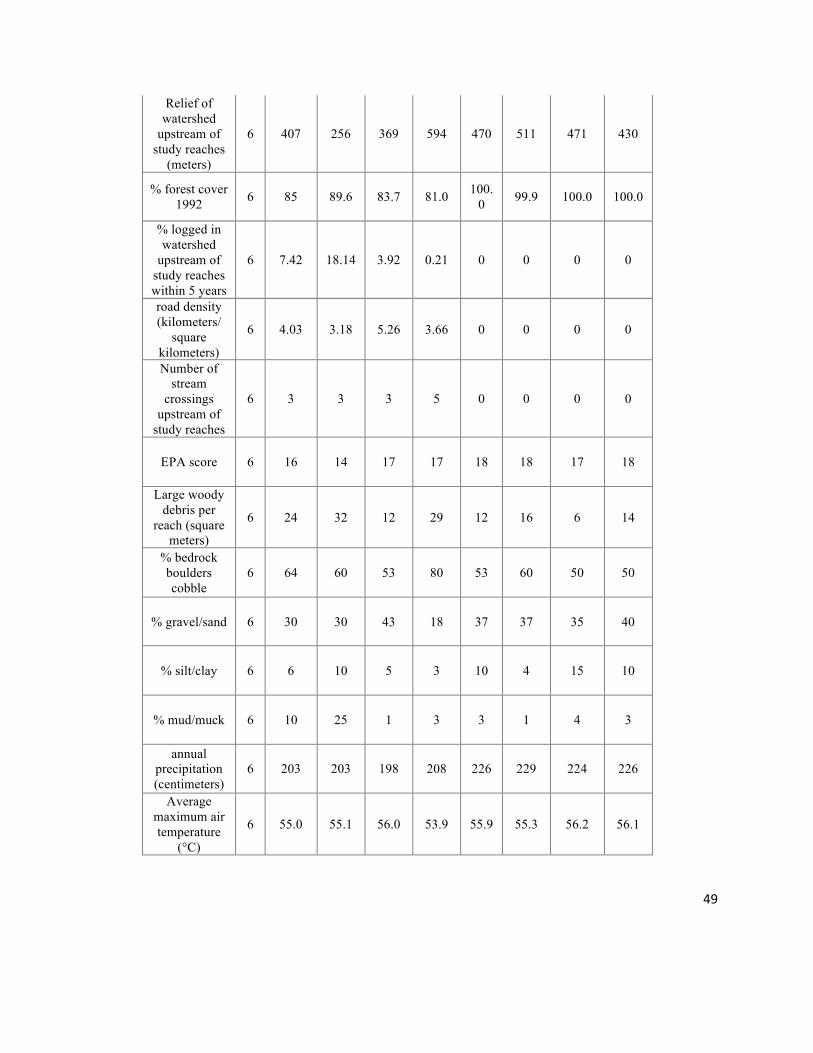
49  

 

Relief of watershed

upstream of study reaches

(meters)

6 407 256 369 594 470 511 471 430

% forest cover 1992 6 85 89.6 83.7 81.0 100.

0 99.9 100.0 100.0

% logged in watershed

upstream of study reaches within 5 years

6 7.42 18.14 3.92 0.21 0 0 0 0

road density (kilometers/

square kilometers)

6 4.03 3.18 5.26 3.66 0 0 0 0

Number of stream

crossings upstream of

study reaches

6 3 3 3 5 0 0 0 0

EPA score 6 16 14 17 17 18 18 17 18

Large woody debris per

reach (square meters)

6 24 32 12 29 12 16 6 14

% bedrock boulders cobble

6 64 60 53 80 53 60 50 50

% gravel/sand 6 30 30 43 18 37 37 35 40

% silt/clay 6 6 10 5 3 10 4 15 10

% mud/muck 6 10 25 1 3 3 1 4 3

annual precipitation (centimeters)

6 203 203 198 208 226 229 224 226

Average maximum air temperature

(°C)

6 55.0 55.1 56.0 53.9 55.9 55.3 56.2 56.1

50  

 

Average minimum air temperature

(°C)

6 36.5 36.3 37.0 36.4 36.1 35.6 36.4 36.4

Average soil permeability centimeters/

hour

6 6.9 7.1 6.5 7.2 7.1 7.9 6.6 7.1

Non-reference streams had greater variability in water quality parameters of

turbidity, TDS, SSC, and conductivity, and stream habitat conditions of canopy cover,

embeddedness, and pebble counts (Table 4, Figure 7). Streamflow and conductivity were

also more variable in non-reference streams, though streamflow and size of watershed

upstream of study reaches were strongly correlated, as were conductivity and TDS. EPA

rapid habitat assesment scores were slightly more variable in non-reference streams.

While water quality and habitat parameters in non-reference streams showed more

variability than in reference streams, macroinverterbrate assemblages showed patterns on

NMDS ordination suggesting less variability in macroinvertebrate assemblages in non-

reference streams- i.e., more tightly grouped and homogenous community structures in

non-reference streams compared to those of reference streams.

51  

 

Table 4: Mean, median, and range of values for water quality and environmental parameters in non-reference and reference streams. Greater variability is displayed in non-reference streams in turbidity, total dissolved solids (TDS), conductivity, suspended sediment concentrations (SSC), flow, canopy cover, embeddedness, pebble counts, and EPA rapid habitat assessment scores.

Parameter

Mean

values: non-

reference

Median values:

non-reference

Mean

values: referenc

e

Median values:

reference

Variability: Range of

values non-reference

streams

Variability: Range of values in reference streams

Turbidity (NTU) 0.97 0.97 0.54 0.55 0.5 - 2.15 0.27 - 0.82

TDS (milligrams/

liter) 0.04 0.04 0.03 0.03 0.02 - 0.06 0.02 - 0.04

Conductivity (µS/

centimeter) 59.04 65.57 48.04 47.86 27.25 - 84.5 31 - 58.5

SSC (milligrams/

liter) 1.42 1.13 0.54 .48 0.48 - 3.16 0.24 - 1.04

Flow (cubic feet/second) 0.97 0.86 0.35 0.28 0.17 - 2.8 0.04 - 0.95

Temperature (Celsius) 8.19 8.06 9.71 9.74 7.38 – 8.73 9.4 – 9.96

Dissolved Oxygen (%) 107.8 109.03 98.2 94.04 101.63 -

111.28 90.65 – 109.42

Canopy cover (%) 85 89.5 82 83.5 65 - 94 75 - 87

Embeddedness (%) 21.2 13.5 20.7 22 7 - 42 14 - 29

Pebble counts (geometric

mean diameter,

millimeters)

44 45 47 46.5 29 - 42 44 - 50

EPA rapid habitat scores

(out of possible 20

points)

15.8 16.5 17.5 17.5 14 - 17 16 - 18

Highest average turbidities occurred in the non-reference streams of Canine and

Dog creeks, with a combined average turbidity of 1.16 NTU (n=8). Pup Creek (also non-

reference) had an average turbidity of 0.58 (n=4), the lowest average turbidity of the non-

52  

 

reference streams and closer in similarity to reference streams. Alice Creek had the

lowest average turbidity of the reference streams: 0.32 NTU (n=4); Doris and Ora creeks

(also reference streams) had similar range of average turbidity values, and had a

combined average turbidity of 0.64 NTU (n=8). In sediment-related parameters, Pup

Creek had average values more similar to those of reference streams for turbidity, TDS,

EPT and MFBI. Alice Creek had average values similar to those of non-reference creeks

in percentages of both gatherer-collectors and shredders. Pup Creek had the largest

average flow values of all streams (1.8 cfs); non-reference streams Canine and Dog

creeks had similar average flows to those of reference streams Alice and Doris creeks

(0.54 and 0.43 cfs average flows, respectively). Ora Creek had lowest average flows

(0.24 cfs).

Average precipitation for the seven days prior to spring sampling events was 3.3

cm for non-reference areas and 1.5 cm in reference areas. For the two days prior to spring

sampling events, precipitation accumulation was 0.5 cm in non-reference areas and zero

cm in reference areas. There was no average precipitation accumulation for the week

prior to early summer sampling events in non-reference and reference areas. Average

precipitation accumlation seven days prior to late summer sampling was 1.8cm in non-

reference streams and 1.3cm in reference streams; there was no accumlation two days

prior to sampling. Average precipitation accumulation for the seven days prior to fall

sampling events was 5.3 cm in non-reference areas and 4.1 cm in reference areas.

Average precipitation accumulation for two days prior to fall sampling events was 1.1 cm

in non-reference areas and 1.5 cm in reference areas.

53  

 

Upstream vs. downstream

Non-reference sites had a greater increase in stream temperature from

downstream to upstream than did reference sites (p=0.01), and increased an average of

0.6 degrees Celsius while reference streams were 0.2 degrees cooler on average. Canine

Creek had the largest average temperature increases from upstream to downstream (an

average increase of 0.65 degrees Celsius). Pup Creek had the smallest increase of 0.45

degrees Celsius.

My hypothesis that sediment-related water quality parameters, stream habitat

measurements, and macroinvertebrate index scores would indicate increased levels of

fine sediments from upstream to downstream in non-reference sites was not supported.

No differences were found in magnitude of change from upstream to downstream in

reference vs. non-reference streams in: turbidity, conductivity, TDS, DO, flow, EPA

rapid assessment scores, embeddedness, or pebble counts. No significant differences

were found in magnitude of change from upstream to downstream in non-reference vs.

reference streams for any macroinvertebrate functional feeding groups, EPT or MFBI

indices, habitat preferences, abundance, diversity or species richness. No differences

were found in predators, filterer/collectors, or scraper functional feeding groups in

magnitude of change from upstream to downstream in non-reference vs. reference

streams. No differences were found between downstream and upstream for Shannon’s or

Simpsons diversity indices, nor in Shannon entropy or Pielou evenness.

All water quality parameters tested for significant differences between reference

and non-reference streams and between magnitude of change in reference vs. non-

54  

 

reference streams had an n=24 except for SSC, embeddedness, pebble counts, and

canopy cover, which were n=6.

Macroinvertebrate Assemblages

Macroinvertebrate Metrics

Macroinvertebrate assemblages in non-reference streams were more abundant in density

and taxa number. Average abundance was approximately 3.9 times higher in non-

reference streams than in reference streams, a marginally significant difference (p=0.05;

Table 5). Average total abundance was 1079 individuals in non-reference streams, almost

four times as great as abundance in reference streams (Figure 8). Average

macroinvertebrate densities were approximately 5994 individuals per square meter in

non-reference streams and 1533 individuals per square meter in reference streams. Pup

Creek (non-reference) had the highest abundance of all streams, approximately one and a

half to two times as great as average abundances of Canine and Dog creeks (non-

reference creeks). Alice Creek had the highest abundance of reference creeks, 1.2 times

larger than Ora Creek and four times larger than Doris Creek. Total number of individual

macroinvertebrates counted was 8100 (7941 keyed to family or most appropriate

taxonomic level).

55  

 

Figure 8: Boxplots depicting abundance, richness, MFBI scores, EPT scores, Plecotpera as a percent of EPT portion of sample, and Plecoptera as a percent of whole samples. Lower MFBI scores suggest better water quality. Green boxplots represent reference streams, yellow represent non-reference streams.

Taxa richness was higher in non-reference streams; this difference was marginally

significant (p=0.05). A total of 43 taxa were found across all sites, with an average of 33

taxa in non-reference streams and 28 taxa in reference streams (Figure 8). Average taxa

richness in non-reference streams ranged from 32 to 35 families; taxa richness in

reference streams ranged from 23 to 31 families.

56  

 

Table 5: Selected macroinvertebrate metrics in non-reference and reference streams.

The top two dominant taxa in all sites combined were Chironomidae and

Nemouridae, and comprised 18.4% of samples (Table 6). The top two dominant taxa in

non-reference streams were Chironomidae and Ostracoda, which comprised 24 percent of

57  

 

macroinvertebrate taxa. In reference streams, the top two most dominant taxa were

Nemouridae and “slenderflies” (Capniidae and Leuctridae combined). These two taxa

comprised 24.1 percent of macroinvertebrate samples in reference streams. Dominant

taxa calculations included two taxa which were not common to all streams, i.e.,

Ostracoda and Gastropoda were present in five of six streams, but had high NMDS

values and were significant in the ordination plot. Taxa that occurred in non-reference

sites only were: Veronida, Psephenidae, Pelecorhynchidae, and Limnephilidae; taxa that

occurred in reference sites only were: Ptilodactylidae, Hydroptilidae, and Corydalidae.

Table 6: Dominant taxa in all study streams, reference streams, and non-reference streams. The Plecoptera families of Capniidae and Leuctridae were combined into the single category of “slenderflies”. Dominant taxa- all streams

% Reference sites- dominant taxa

% Non-reference- dominant taxa

%

Chironomidae 10.4 Peltoperlidae 12.1 Chironomidae 13.6 Nemouridae 8 Nemouridae 12.0 Ostracoda 11.4 Peltoperlidae 7.3 “slenderflies” 7.6 Heptageniidae 7.2 “slenderflies” 7.2 Gastropoda 7.3 “slenderflies” 6.7 Ostracoda 6.9 Chironomidae 7.2 Rhyacophilidae 6.7 Gastropoda 6.4 Chloroperlidae 6.5 Elmidae 5.6 Heptageniidae 5.9 Baetidae 4.6 Gastropoda 5.5 Chloroperlidae 5.7 Leptophlebiidae 4.5 Chloroperlidae 4.8 Rhyacophilidae 5.5 Heptageniidae 4.5 Baetidae 4.0 Baetidae 4.3 Rhyacophilidae 4.3 Nemouridae 4.0

Macroinvertebrate assemblages were dominated by pollution sensitive taxa.

Average EPT index scores were 71.2 in reference streams, and approximately 28% higher

than those of non-reference streams. The difference was statistically significant (p=0.03).

Plecoptera averaged 22 percent of macroinvertebrates in non-reference samples and 41

58  

 

percent of reference samples as a percentage of the entire sample, and was higher in

reference samples (p=0.01). Percent plecotera of the EPT portion of reference samples

was 44 percent in non-reference stream samples and 58 percent of reference samples,

though the difference was statistically marginal (p=0.10; Figure 8). Average MFBI index

scores were 3.00 and 3.91 in reference and non-reference streams, respectively. However,

the difference in MFBI scores was not significant (p=0.09) (Table 5).

Macroinvertebrate groups classified on their functional feeding modes were

significantly different between non-reference and reference sites. Collector-gatherers

comprised 44 percent of non-reference macroinvertebrate samples, approximately 1.9

times higher than those of reference sites. The difference was statistically significant

(p=0.02). Thirty five percent of macroinvertebrates in reference streams were shredders,

approximately 2.3 times higher than non-reference streams. The difference was

marginally significant (p=0.05; Table 5; Figure 9). Chironomids comprised an average of

13.6 percent of non-reference samples and 7.2 percent of reference samples. Chironomids

in Pup Creek comprised 70.5% of all chironomids in non-reference streams. Chironomids

in Alice Creek comprised 71.0% of all chironomids in reference streams. Dipterans

comprised an average of 2.0 percent of non-reference samples and 1.4 percent of

reference samples.

59  

 

Figure 9: Macroinvertebrate functional feeding groups in reference (green box plots) vs. non-reference (yellow box plots) sites. Percent of gatherer-collectors and shredders were different in reference vs. non-reference streams (p-values = 0.02 and 0.05, respectively).

Average values were similar in diversity and evenness indices in non-reference

vs. reference sites. No differences were found in reference vs. non reference streams for

Shannon’s or Simpsons diversity indices, Shannon’s entropy, Pielou evenness, predators,

filterer/collectors, or scraper functional feeding groups. Average Shannon’s diversity

scores were 16.07 and 15.45 for non-reference and reference streams, respectively.

Simpsons diversity scores were 10.92 and 10.63 for non-reference and reference streams,

respectively.

Pup Creek had the lowest average MFBI score (3.26) and highest average EPT

score (64) of the non-reference streams, with values closer to those of reference streams

than other non-reference streams. Canine Creek, which had the lowest streamflow of the

non-reference streams, had the highest MFBI (4.31) and lowest average EPT (42) scores

60  

 

of non-reference creeks. Ora Creek had the highest average MFBI score (3.26) and the

lowest average EPT score (61) of the reference creeks. Alice and Doris creeks had similar

MFBI and EPT scores, with overall averages of MFBI = 2.9 and and EPT = 76.

Average percentages of gatherer-collectors and shredders in Alice Creek

(reference) were more similar to non-reference streams. Gatherer-collectors and

shredders had similar average percentages across non-reference streams; Doris and Ora

creeks (reference streams) also had similar average percentages to each other. Of the non-

reference streams, Canine Creek had the highest percentage of gatherer-collectors (51

percent); Dog and Pup creeks had similar percentages of gatherer-collectors (42 and 39

percent, respectively). Ora Creek had the lowest percent of gatherer-collectors (13

percent), while Alice Creek had the highest (41 percent). Alice Creek had the lowest

percentage of shredders (22 percent), and Doris Creek had the highest percentage of

shredders (48 percent). Chironomids comprised 42 percent of the gatherer-collector guild

in non-reference streams, and 32 percent in reference streams. Gatherer-collectors in Pup

Creek comprised 48 percent of gatherer-collectors in all non-reference streams. Gatherer-

collectors in Alice Creek comprised 72% of all gatherer-collectors in reference streams.

Macroinvertebrate Assemblage Distributional Patterns

Reference and non-reference streams had significantly different macroinvertebrate

assemblages. NMDS analysis showed that reference sites generally fall along the left half

of the NMDS plot, and non-reference sites on the right (Figure 10). ANOSIM tests

indicated that the difference was significant (p=0.007).

61  

 

Non-reference sites are more tightly grouped together on the ordination plot

compared to reference streams, showing that macroinvertebrate assemblages in non-

reference streams are more homogenous. Reference streams are further apart relative to

each other, and have more dissimilar assemblages.

Figure 10: Dominant taxa on the NMDS ordination plot based on macroinvertebrate assemblages in all study sites. Sites 1-6 are non-reference sites and 7-12 are reference sites and are represented by circles and triangles, respectively; downstream locations are represented by odd numbers and upstream sites are represented by even numbers. ANOSIM test showed significant differences in reference vs. non-reference sites (p=0.007).

Taxa strongly associated with macroinvertebrate distributional patterns on the

NMDS I axis that were associated with non-reference sites were: Empididae,

Philopotmidae, Ephemerellidae, Oligochaeta, Ostracoda, and Veronida (Table 7). Taxa

strongly associated with distributional patterns on the NMDS I axis that were associated

62  

 

with reference sites were: Simulidae, Ceratopogonidae, Hydroptilidae, Nemouridae,

Peltoperlidae, and Brachycentridae. Taxa strongly associated with NMDS II axis were:

Dixidae, Gastropoda, Hydracarina, Apataniidae, Baetidae, Goeridae, Heptageniidae, and

Psychodidae. Significant and marginally significant taxa largely overlapped with

dominant taxa, but were not identical (Figure 11). Some taxa strongly associated with

distributional patterns on the NMDS 1 and 2 axes also influenced macroinvertebrate

metrics, and trends are clearly visible across study sites in reference and non-reference

streams (Figures 12 and 13).

Table 7: NMDS 1 and 2 scores, R2  values, and p-values for significant macroinvertebrates on NMDS ordination plot. Single asterisks indicate significance; two asterisks indicate lowest p-values. Vectors   NMDS1   NMDS2   R2   Pr(>r)      Hydroptilidae   0.928   -­‐0.373   0.863   0.004   **  Peltoperlidae   0.787   -­‐0.617   0.788   0.004   **  Ephemerellidae   -­‐0.903   0.430   0.736   0.005   **  Heptageniidae   -­‐0.470   0.883   0.687   0.005   **  Ceratopogonidae   0.989   -­‐0.151   0.638   0.015   *  Gastropoda   -­‐0.080   -­‐0.997   0.637   0.004   **  Ostracoda   -­‐0.861   -­‐0.509   0.594   0.015   *  Hydracarina   -­‐0.116   -­‐0.993   0.594   0.015   *  Dixidae   0.116   -­‐0.993   0.565   0.028   *  Oligochaeta   -­‐0.899   0.4381   0.564   0.017   *  Nemouridae   0.900   0.435   0.554   0.026   *  Simulidae   0.999   0.038   0.546   0.041   *  Psychodidae   -­‐0.641   0.768   0.515   0.037   *  Apataniidae   0.176   -­‐0.984   0.500   0.050   *  Brachycentriade   0.717   -­‐0.698   0.496   0.047   *  Empididae   -­‐0.998   0.069   0.494   0.046   *  

63  

 

Figure 11 (A – H): Bubble plots of dominant taxa on NMDS ordination based on macroinvertebrate assemblages at all study sites. Taxa are shown in order of most dominant for the first eight most dominant taxa. Reference streams are depicted in red; non-reference in black.

64  

 

Figure 12: Bubble plots showing abundance on the left and richness on the right. Both are based on NMDS ordination plot of macroinvertebrate community assemblages at each study site. Reference streams are depicted in red circles, non-reference streams in black.

Figure 13: Bubble plots showing functional feeding groups of gatherer/collectors and shredders on NMDS ordination of macroinvertebrate community assemblages at each study site. Reference streams are depicted in red circles, non-reference in black. The percentage of gatherer-collectors was higher in non-reference streams (p=0.02), while the percentage of shredders was higher in reference streams (p=0.05).

65  

 

Macroinvertebrate Assemblage Distributional Patterns and Environmental Variables

Both anthropogenic variables and environmental conditions were associated with

overall macroinvertebrate distributional patterns (Table 8). Linear vector fitting analysis

indicated that watershed land use and land cover (road density and percent forest cover

(from 1992 dataset)), water quality (TDS, conductivity, stream temperature, and percent

silt/clay), annual precipitation, and relief of delineated watershed were associated with

changes in macroinvertebrate assemblages (Figures 14 and 15). These associations were

significant or marginally significant (Table 8). Turbidity, percent of mud/muck, size of

watershed upstream of study sites, number of stream crossings, and the presence of

adjacent logging within five years (Y or N) had a very weakly association with

macroinvertebrate assemblages.

66  

 

Figure 14: Envfit of environmental variables on the NMDS plot based on dissimilarities of macroinvertebrate community assemblages across all study sites. Environmental variables displayed are significant or marginally significantly associated with macroinverterbate assemblages on NMDS ordination. Black circles represent non-reference sites; red circles represent reference sites.

67  

 

Figure 15: NMDS plot with all environmental variables, regardless of strength of association or signfiicance.

Increased road density was strongly associated with non-reference

macroinvertebrate assemblage patterns. Road density had the highest absolute value of all

NMDS I scores (-0.9995) as well as a low p-value (p=0.029). Envfit overlay shows a

strong association between increased percentage of historic forest cover (1992 dataset)

and macroinvertebrate community structure patterns (NMDS I = 0.95 and p=0.068). The

number of stream crossings was moderately associated with macroinvertebrate

assemblage patterns (p=0.21), and had NMDS I and II scores of -0.76 and 0.65,

respectively, but also had moderate to strong Pearson’s correlation coefficient values with

road density (0.71), and was omitted as it nearly overlapped with road density on the

ordination plot. Envfit shows a weak association (p=0.12) with the presence of recent

68  

 

logging within five years adjacent to study sites (Yes vs. No). No significant difference

was found in the ANOSIM test based on the difference between the two groups (Yes or

No for presence of adjacent logging within five years).

Environmental conditions which had a strong or moderately strong association

with macroinvertebrate community assemblages using envfit on the NMDS plot included:

TDS, annual precipitation, conductivity, stream temperature, percent silt/clay, flow, and

relief. Increased TDS was strongly associated with reference macroinvertebrate

community structure patterns, and had the second-highest NMDS I value of both natural

and anthropogenic envfit variables. TDS and conductivity had a Pearson’s correlation

coefficient of 0.90, as TDS is based on conductivity. Increasing stream temperature was

strongly associated with assemblages patterns in reference stream along the NMDS I

axis. Silt/clay as a percent of streambed composition had moderate influence on both the

NMDS I and II axes, and was approximately opposite to increasing flow, though flow

was more influential along the NMDS II axis than on the NMDS I axis. Relief was

strongly influential on the NMDS II axis, and was associated with assemblage patterns in

both reference and non-reference streams. Turbidity, percent mud/muck, and watershed

size upstream of study reach showed moderate associations with macroinvertebrate

assemblage patterns, but had relatively high p-values (turbidity and percent mud/muck)

or were correlated with other variables (watershed size upstream and flow had a

Pearson’s correlation coefficient of 0.93 and nearly overlapped; flow had a larger NMDS

I value and so watershed size was omitted on NMDS plots). ANOSIM tests did not find

69  

 

macroinvertebrate structure patterns to be significantly different based on aspect

(p=0.28).

Table 8: NMDS I and 2 scores, R2 values, and p-values for environmental conditions associated with macroinvertebrate assemblage patterns on the NMDS ordination plot. Vectors that were significant are denoted with asterisks (*); marginally significant vectors are denoted with periods (.). Vectors NMDS1 NMDS2 R2 Pr(>r) Percent silt and clay 0.762 -0.647 0.564 0.0280 * Road density -0.999 0.0307 0.554 0.0310 * Conductivity -0.975 -0.221 0.482 0.039 * Annual precipitation 0.997 0.0837 0.467 0.058 . Percent forest cover (1992 data) 0.953 -0.303 0.464 0.065 . Stream temperature 0.988 -0.153 0.450 0.074 . Relief 0.466 0.885 0.448 0.069 . Total dissolved solids -0.999 -0.0422 0.417 0.065 .

Pearson’s correlation coefficients were moderate for associations between the

percent of the watershed logged upstream of study sites within the past five years, and

sediment-related water quality parameters including conductivity, TDS, turbidity,

embeddedness, and pebble counts; the correlations were 0.75, 0.72, 0.76, 0.75, and -0.89,

respectively (n=6; Figure 16).

70  

 

Figure 16: Correlation matrix showing Pearson’s correlation coefficients for selected environmental conditions, from top right to bottom left: conductivity, total dissolved solids (TDS), turbidity, embeddedness, pebble count (geometeric mean diameter in millimeters), percent of watershed logged within the last five years (upstream of study reaches), road density, and percent of forest cover (1992 data). The larger the correlation, the larger the phont of the Pearson’s correlation value (n=6).

71  

 

Chapter 4: Discussion

Responses of Macroinvertebrate Assemblages to Forest Management

Associations between land use, fine sediments, and changes in macroinvertebrate

metrics and community assemblages were apparent at the reference vs. non-reference

scale. It is likely that macroinvertebrates are responding, at least in part, to past logging

and high road densities in non-reference streams. Fewer indications were found that

recent logging may be affecting water quality and macroinvertebrates. Pearson’s

correlation coefficients show that the percent of recent logging upstream of study sites

was correlated with several measures of fine sediments, suggesting that recent land use

may be affecting water quality. However, Pearson’s correlation coefficients were based

on n=6, and so these results should be interpreted with caution due to the small sample

size. Macroinvertebrates in downstream non-reference sites clustered together in tow of

three non-reference streams, as did those upstream, suggesting possible responses to

similar recent environmental stressors. Stream temperatures increased from upstream to

downstream in non-reference sites, possibly in response to recent selective logging. Even

though temperatures were collected only during sampling events and no continual data

were collected in this study, the history of widespread and continuing temperature

standard exceedances in the area indicates that further research investigating how

selective logging may affect temperature in the Clackamas is warranted. Temperature

increases in non-reference streams may be the result of time of day of sampling.

However, reference and non-reference streams were sampled in the same standardized

fashion at very similar times of day. No other differences in water quality parameters

72  

 

were found from upstream to downstream, possibly because water quality was

sufficiently protected, or because signals from land use impacts may be obscured by a

several factors, including upstream confounding factors such as past logging and roads,

and natural variability.

Macroinvertebrate Metrics: Abundance, Density, and Richness at Reference vs. Non-reference Sites

Increased macroinvertebrate abundance and density in non-reference streams in

this study was likely driven by increased nutrient availability in relation to land use

impacts. Increases in secondary production in relation to logging have generally been

attributed to greater algal growth in streams in response to increased available light

related to larger canopy openings, with some streams experiencing shifts from

allochthonous to autochthonous primary production (Richardson and Danehy 2007,

Sponseller et al. 2001, Stone and Wallace 1998, Webster et al. 1992). However,

silvicultural prescriptions in non-reference sites in my thesis research included upland

selective logging and riparian buffers with limited cutting, with non-reference sites

having denser average canopy cover compared to reference sites. Thus, it is unlikely that

increased algal production in response to increased light is the sole or dominant driver of

the greater macroinvertebrate density found in non-reference areas. While most research

has focused on macroinvertebrate response to clearcut logging with small or no riparian

buffers, some studies have investigated selective logging. For example, Miserendino and

Masi (2010) investigated macroinvertebrate response to selective logging with riparian

buffers and also found increased total macroinvertebrate density, though the authors did

73  

 

not speculate about the possible mechanisms for this increase they noted that at least one

of these streams also had increased sediment levels. Additionally, not all research on

clearcut logging found increases in macroinvertebrate abundance and density to be linked

solely to increased light resources stimulating autochthonous energy production. Some

studies found secondary production increases to be at least partly associated with higher

stream temperatures, increased nitrogen and phosphorus availability (Sponseller et al.

2001, Webster et al. 1992), and shifts from conifer to deciduous tree species composition

(Piccolo and Wipfli 2002, Progar and Moldenke 2009). In deciduous forests at Coweeta,

Stone and Wallace (1998) found higher secondary production as well as more rapid

processing of leaf litter in streams in logged deciduous forests compared to undisturbed

streams. They postulated that this rapid processing of leaves might limit microbial

colonization opportunities, thereby increasing nutrient availability and, in turn, the

greater secondary production found in disturbed streams. In research on adult aquatic

emergent insects, Progar and Moldenke (2009) found that headwater streams in young,

previously clearcut conifer forests produced a 1.5 fold higher density and biomass of

insects than did streams in mature forests. They attributed this increase to either: labile

nutrient availability in deciduous leaf letter, increased insolation providing for increased

periphyton production, or a combination of these factors. In the Fish Creek Watershed

Analysis, the USFS (1994) suggests that increased summertime stream temperatures in

Fish Creek may be affecting nutrient enrichment in Fish Creek, the stream that one of my

non-reference creeks (Dog Creek) drains into. Stone and Wallace (1998) found that

macroinvertebrate abundance was still elevated 16 years after logging, which supports the

74  

 

theory that the increased abundance in non-reference streams in this study may be related

to past logging as well as current land use impacts including road density, other road-

related activities, and recent logging. Sponseller et al. (2001) emphasized the importance

of scale in analysis, and noted that macroinvertebrate density was related at the 2000

meter sub-corridor scale to non-forested land. Contrary to results in this study, other

studies have found macroinvertebrate abundance, density, and richness to decrease in

relation to increasing fine sediments associated with logging (Angradi 1999, Zweig and

Rabeni 2001, Waters 1995). It is not clear why increased sediments are associated with

decreased secondary production in some studies and not in others. Possibly, increased

availability of nutrients and warmer stream temperatures may stimulate secondary

productivity, but only up to a threshold, after which detrimental impacts may exceed

benefits and sufficient portions of taxa experience negative impacts, resulting in declines

in total abundance, density, and richness. If such a threshold exists, it is likely that it

would interact with fine sediments, gradient, streamflow, streambed substrates, and other

environmental conditions in complex interactions producing great variability and making

predictions concerning macroinvertebrate abundance and density challenging.

Natural variability among stream sites, including differences in canopy species

and size of stream, may also be related to increased secondary production in this study.

For example, greater presence of deciduous vegetation (based on qualitative

observations) and larger streamflows in Pup Creek (non-reference) and in Alice Creek

(reference) seem to be linked to the particularly heightened macroinvertebrate abundance

in those streams. In particular, Pup Creek contained the largest average macroinvertebrate

75  

 

abundance and density, and had the highest deciduous tree species presence and largest

streamflows. Herlihy et al. (2005) noted increased abundance of Ephemeroptera,

particularly Baetis, in association with increasing streamflows. While this study did not

identify macroinvertebrate taxa to genera, the increase in Baetis in Herlihy et al. (2005)

may be reflected in the increase in Baetidae and other Ephemeroptera families found in

this study in relation to faster moving waters. In addition, Piccolo and Wipfli (2002)

found that young-growth red alder stands exported far higher densities of

macroinvertebrates than did young-growth conifers. Willacker et al. (2009) also found

that deciduous streams had greater abundance, taxa richness, diversity, and unique taxa

compared to conifer (hemlock) dominated streams. However, the trend of increased

abundance and density in non-reference sites continues to be present even if Pup Creek is

excluded, suggesting that increased deciduous cover and streamflow are not related to

increased macroinvertebrate abundance in other non-reference streams.

Contrary to results in this study, Zhang et al. (2009) and Waters (1995) found

decreasing taxa richness in relation to logging, though their studies examined clearcut

logging. Zweig and Rabeni (2001) found that taxa richness declined with increasing

stream sediment deposits. However, Progar and Moldenke (2009) did not find differences

in taxa richness between mature forests and young stands that had been clearcut 10 years

before. Taxa richness in non-reference sites in this study may have been related to

increased nutrient availability, with instream conditions retaining sufficiently high water

quality to maintain the presence of most sensitive species.

76  

 

Macroinvertebrate Metrics: EPT and MFBI at Reference vs. Non-reference Sites

Lower EPT abundance and higher MFBI scores may indicate poorer water quality

in relation to anthropogenic impacts in non-reference streams compared to reference

streams, though the increase in MFBI scores was only marginally statistically significant.

Zweig and Rabeni (2001) and Waters (1995) found EPT abundance and density to be

negatively correlated with increased fine sediments. Increased fine sediment levels in

non-reference streams may be partly responsible for the lower EPT and higher MFBI

scores in non-reference streams, as these streams also contained greater turbidity, TDS,

and SSC than reference streams. In research focusing on selective logging, Flaspohler et

al. (2002) found a negative correlation with year of logging and EPT abundance, contrary

to their original expectations that selective harvest would not produce significant

responses. However, decreased EPT abundance was not correlated with fine sediments in

their study. Brook char (Salvelinus fontinalis) were negatively correlated with year of

selective harvest, and they noted that streams with high EPT scores also had intermediate

total macroinvertebrate densities, possibly suggesting a relationship between secondary

productivity potential and habitat quality which may exert distinct influences on

macroinvertebrate composition and density (Flaspohler et al. 2002). Contrary to the

results in this study, Progar and Moldenke (2009) did not find changes in EPT density,

richness, or biomass in insects from streams in areas clearcut 10 years before compared

to those in mature forests. Gravelle et al. (2009) also found that logging and roads did not

seem to affect EPT indices, and that any statistical differences present in their study were

small and attributable to natural variability. Barbour et al. (1999) reported that MFBI

77  

 

scores increased and EPT density decreased with increasing perturbation. Differences in

EPT and MFBI sensitivity to perturbation may vary in relation to a wide range of factors,

including natural variation among sites, intensity of logging, and other influences. It may

also be possible that the differences found in macroinvertebrate metrics in this study may

be related to natural variability or other unknown factors, and that apparent associations

with logging and roads are coincidental and partly an artifact of small sample size.

Additionally, Hilsenhoff (1988) cautioned that the family-level identification of

macroinvertebrates, while useful for rapid assessments, may not provide sufficient

precision and may produce erroneous conclusions regarding water quality, and is not

meant to replace MFBI indices. Zweig and Rabini (2001) found that identification to the

genus level was necessary for accurate determination of MFBI scores, and that family

level identification may not be sufficient, especially with Chironomid identification and

associated tolerance levels because some Chironomidae genera are sensitive to sediments

and other disturbances, while others are very tolerant. However, other studies have found

little difference in effectiveness between family and genus level identification for

determining stream impairment, including distinctions between non-impaired, moderately

impaired, and severely impaired waters (Hewlett 2000). Lenat and Resh (2001) noted that

while family and genus/species biotic indices were highly correlated in North Carolina

studies, family-level identification can result in erroneous conclusions. Genera tolerance

scores may vary widely within a single family, producing intermediate family tolerance

scores that may not accurately represent genera or conditions present. Bailey et al. (2001)

found that family level identification produced very similar results to genus level

78  

 

identification in multivariate analyses, and for areas with relatively low diversity.

However, they found that genus/species identification was beneficial for specific

indicators of particular pollutants (Bailey et al. 2001). It is possible that MFBI scores may

have yielded erroneous conclusions regarding water quality in this study. However, given

that EPT indices also suggest poorer water quality, and that Plecoptera and shredders

decreased in reference sites while gatherer-collectors increased, it seems likely that the

multiple metrics suggesting impaired water quality have accurately detected an actual

deviation in conditions compared to reference streams.

Significant and nearly-significant smaller percentages of Plectoptera in both

overall sample and in the EPT portion of samples in non-reference streams may also

suggest possibly poorer water compared to reference streams. Percent plecoptera has

been found to decrease in relation to increasing perturbation (Barbour et al. 1999, Herlihy

et al. 2005), including logging (Wood and Armitage 1997). Progar and Moldenke (2009)

also found greater Plecoptera biomass in emergent aquatic insects in mature forests vs.

those in forests clearcut 10 years previous.

Macroinvertebrate Metrics: Gatherer-collectors at Reference vs. Non-reference Sites

Higher average percent of gatherer-collectors in non-reference streams in this

study may be related to increased sediment levels in non-reference streams. Greater

turbidity, TDS, and SSC indicate greater levels of sediment in non-reference streams,

though TDS and SSC were only marginally significant, and all sediment-related

parameters had relatively low values. Kreutzweiser et al. (2005) found that selective

79  

 

logging with 42% basal area removal produced shifts in macroinvertebrate structure,

including increases in several gatherer taxa, which appeared to be linked to an increase in

fine organic sediment deposition. It is difficult to compare the intensity of the project

Kreutzweiser studied to the logging in this study due to the different metrics provided

(i.e., basal area vs. canopy cover and relative density), though both were classified as

“moderate” thins. Silvicultural prescriptions in this study included logging in riparian

areas, as well as areas of “gaps” and “heavy thins” with as low as 20% relative density

interspersed across the landscape (USFS 2006), which seem to suggest logging

prescriptions approximately equal to those found in Kreutzweiser’s research. Research at

Coweeta regarding clearcut logging, as summarized by Webster et al. (1992), also found

that annual instream sediment transport clearly exceeded reference levels after logging,

even in catchments where no roads or skid trails were built and no logs were removed. In

other catchments containing roads, the majority of instream sediment transport was

attributed to road-related activities, with some affected streams continuing to export

excess sediments eight years later. In addition, instream sediments were shown to have a

higher fraction of organic material compared to undisturbed streams, which may have

been associated with increased collector abundance (Webster et al. 1992). Stone and

Wallace (1998), also studying streams at Coweeta Experimental Forest, found collectors

to have three times greater abundance than undisturbed streams, though this included

filterer-collectors as well as gatherer-collectors. The Fish Creek Watershed Analysis

(USFS 1994) suggested that decreased retention of coarse organic matter in Fish Creek

80  

 

may be shifting macroinvertebrate functional feeding groups from shredders to collector-

gatherers.

Chrinomids are part of the gatherer-collector functional feeding group, tend to be

associated with higher sediment environments (Wood and Armitage 1997), and are

generally considered to be tolerant (Herlihy et al. 2005). Overall, non-reference sites in

this study have a larger average percentage of Chironomids, as well as greater turbidity,

TDS, and SSC. Canine and Dog creeks had high sediment-related water quality values

compared to reference streams and to Pup Creek. However, deciduous canopy

composition in some sites and larger stream flow may also have produced increases at

certain sites in some taxa classified as gatherer-collectors. For example, it is possible that

increased presence of deciduous trees, in addition to being partly responsible for overall

abundance in Pup Creek, was partly responsible for the larger percentages of

Chironomids and hence of gatherer-collectors in Pup Creek. Pup Creek contained the

largest percentages of Chironomids, yet had the lowest average values for turbidity, TDS,

SSC, and embeddedness compared to other non-reference streams (differences in

turbidity, TDS, and SSC were significant or marginally significant; differences in

embeddedness were not significant). When Pup Creek is excluded, the non-reference

streams Canine and Dog creeks still contain greater percentages of Chironomids

compared to reference streams, though the difference is not as large. Qualitative

observations of species compositions in Canine and Dog creeks indicate that conifers

dominate riparian areas, with a low abundance of deciduous trees or shrubs. Qualitative

observations during laboratory processing of macroinvertebrates suggest that the majority

81  

 

of Chironomids collected from the downstream portion of Pup Creek were attached to

alder leaves collected in Surber nets during field sampling process. The large increases in

Chironomids in Pup Creek may be related to the much larger deciduous tree (alder)

presence in the downstream study reach of Pup Creek, while increases in Chironomids in

Canine and Dog Creeks may be related to their higher average values of sediment-related

water quality parameters. This might also explain the increased presence of Chironomids

in Alice Creek (reference stream) compared to other reference creeks, as this creek may

have had more deciduous vegetation along study reaches compared to other reference

creeks. While riparian vegetation and tree species compositions were not quantitatively

measured as part of this study, field observations and pictures indicate a large alder stand

is dominant in the riparian area in portions of the downstream study reach of Pup Creek.

Similarly, observations of Alice Creek indicate higher presence of deciduous vegetation,

and downstream portions of Alice Creek were uniquely challenging to access due to the

abundance of low deciduous shrubs. Increased presence of deciduous vegetation may be

due to a number of ecosystem processes and disturbances such as larger stream width

allowing more light onto forest floor, slope instability, increased canopy complexity and

heterogeneity related to old growth structure in reference stands, and past logging in non-

reference stands.

In addition to increased vegetation in riparian areas, larger stream size and faster

flows in Pup and Alice creeks may be partly responsible for the distinct

macroinvertebrate assemblage distributions patterns in these two creeks. Faster stream

flow may be associated with increases in overall abundance of certain families of

82  

 

Ephemeroptera, and particularly the genus Baetis (Herlihy et al. 2005). Increases in

Baetidae were partly responsible for driving overall increases in abundance in this study,

as well as the increases in gatherer-collectors. While this study did not identify

macroinvertebrates to genus level, it is possible that the increases in Baetis as discussed

in Herlihy et al. (2005) may be similarly reflected in this study at the family level. Pup

and Alice creeks had the largest streamflows as well as the highest percentages of Baetids

and the largest overall macroinvertebrate abundances compared to all other creeks. Part

of this increase in abundance was driven by taxa in the Ephemeroptera order, including

Baetidae, Ephmerellidae, and Heptageniidae. Herlihy et al. (2005) also found certain

Ephemeroptera to increase with increasing streamflow, particularly Baetis and two

genera in the Heptageniidae family: Epeorus, and Rithrogena. Angradi (1999) found

Baetidae to increase with increasing percentage of fine sediments. Abundances of

Baetidae, Ephmerellidae, and Heptageniidae increased in non-reference streams in this

study, particularly in Pup Creek, the stream with the largest streamflow. Relative

abundances of Ephmerellidae and Heptageniidae also increased in reference vs. non-

reference streams. All Ephemeroptera families increased in the reference stream with the

largest flow (Alice Creek) compared to other reference streams, also supporting the

assertion that certain taxa of Ephemeroptera increase with increasing streamflow. Overall

relative abundance of Baetidae in this study was slightly greater in reference than non-

reference streams overall, hence, my original hypothesis that Baetids would increase with

increasing sediments and in non-reference sites was not supported.

83  

 

Chironomids and Baetids partly comprise the gatherer-collector functional

feeding group which increased in Pup and Alice creeks, despite the low levels of

sediment present in these creeks. Thus, part of the increase in gatherer-collectors in non-

reference streams may be due to increased deciduous vegetation and larger streamflow,

rather than demonstrating an across-the-board association with increased sediments.

Willacker et al. (2009) found that conifer streams had larger percentages of gatherer-

collectors and lower percentages of shredders and predators compared to deciduous

streams, indicating that influences of deciduous vegetation on gatherer-collectors may be

variable and complex. Even so, the association between increased fine sediment levels

and Chironomids, and collector-gatherers is likely present in the remainder of non-

reference streams, i.e., Canine and Dog creeks. Those streams had increased abundance

and relative abundance of Chironomids as well as higher turbidity, TDS, and SSC, and

EPT and MFBI scores that suggested poorer water quality.

Fine sediments may have complex dynamics not captured in this study due to

infrequent, non-continuous sampling, and by the absence of measurements of streambed

permeability and percent of sediments at depth in the stream bed. Cover et al. (2008)

found that fine sediments may accumulate in the subsurface portions of the stream bed,

even if they don’t accumulate on the surface, particularly in steeper areas. The authors

found that in the steep areas of the Klamath Mountains, accumulation of sediments on

stream surfaces was prevented by the large transport capacity of streams, though gravel

permeability was nevertheless reduced and abundant silt and sand can still accumulate in

these circumstances. It is possible that fine sediments may be accumulating below the

84  

 

surface in interstitial spaces and thus impacting macroinvertebrate assemblage

compositions and abundance, even though low levels of fine sediments were detected in

the water column and on stream bed surfaces. The Fish Creek Watershed Analysis (USFS

1994) noted that stream channels in the Fish Creek Watershed have been  altered by

debris flow and often been scoured to bedrock, which has led to channel simplification,

loss of roughness, loss of habitat, and loss of storage capacity for sediment and nutrients.

The Watershed Analysis also notes that water clarity is extremely high, with not a lot of

fine sediment accumulation, except apparently during early winter storms because the

sediments due to land management and erosion flushed out. Surveys suggest that

degradation in the form of downcutting may be occurring in some areas (USFS 1994).

Pup Creek and other non-reference streams may be experiencing sediment dynamics that

include both scour and as deposition in different areas and in complex patterns. One of

the non-reference streams (Dog Creek) drains into Fish Creek. Other non-reference sites

in this study do not drain into Fish Creek, but are just over the ridge on the other side of

the Fish Creek divide, and are connected to the same road system used above Fish Creek,

and likely had similar intensity of past management. It is also possible that gatherer-

collectors, including Chironomids and Baetids, may also be reacting to other unknown

stressors not addressed or measured in this study.

As expected, the percent of shredder functional feeding group taxa was smaller in

non-reference sites, and may be related to changes in allochthonous input dynamic in

non-reference streams. Shredder assemblages may change in relation to the quality,

quantity, timing, and decomposition rates of these inputs (Lecerf and Richardson 2010).

85  

 

Overall average and median canopy cover is slightly higher in non-reference streams in

this study (the difference is insignificant), which would seem to suggest that non-

reference sites might be more likely to have higher shredder abundance than reference

sites, the opposite of what was found. The mechanism for decreased shredder abundance

in non-reference streams in this study is not entirely clear, though it may be a

combination of factors. For example, taxa within the shredder functional feeding group

are typically sensitive, and therefore may respond negatively to land use impacts

(Barbour et al. 1999). Even though canopy cover in non-reference sites was slightly

greater, changes to the amount, timing, or quality of allochthonous inputs could be

affecting shredder abundance. Additionally, increased algal growth due to increased

nutrient availability related to increases in organic fine sediments and more light

availability may be taking place in some areas, particularly in one non-reference stream.

Dog Creek (non-reference) had the lowest canopy cover of all sites, and some of the

lowest shredder abundances. In their summary of research at Coweeta Experimental

Forest, Webster et al. (1992) noted that shredder abundance decreased in relation to

increasing autochthonous primary production in streams, as did other research (Barbour

et al. 1999, Progar and Moldenke 2009, and Zhang et al. 2009). However, Lecerf and

Richardson (2010) found that shredder abundance and richness decreased in streams with

upland clearcutting regardless of riparian buffer size or treatment, but no changes were

found in shredder abundance or richness in selectively logged reaches. The authors found

increased total dissolved nitrogen in selectively logged reaches (which they believed to

be related to possible increased sediment inputs), and decreased leaf decomposition rates

86  

 

in streams with both clearcut and selectively logged upland areas, regardless of riparian

buffer widths or treatments. Lower decomposition rates in thinned reaches may have

been influenced by increased fine sediments smothering leaf packs and retarding

breakdown processes. Decay rates of organic inputs are complex and depend on type of

leaf/needle litter, fungal presence and interactions, and fine sediment levels (which may

encase/coat leaves and slow decomposition) (Lecerf and Richardson 2010). Haggarty et

al. (2003) also speculated that changes in shredder abundance from logging may be

responses to alteration of detritus supplies. Part of their rationale was that no changes

were found in scraper abundances, which would be expected if algal growth was

increased. No difference was found in this study in the percent of scrapers in non-

reference vs. reference sites, further supporting my speculation that algal growth is not

the sole or primary driver of shifts in macroinvertebrate community structure in non-

reference streams. However, these processes are not well understood, and much of the

research has focused on deciduous rather than coniferous forests. It is not clear if or how

disruption to decomposition processes might affect shredder assemblages in some

streams, though it would seem that possible alterations to processes associated with their

base food resources might also affect them.

Macroinvertebrate Metrics: Dipterans, Oligochaetes, and Turbellarians at Reference vs. Non-reference sites

As expected, Dipteran and Oligochaete relative abundances increased in non-

reference streams. Turbellarians also had greater relative abundance in non-reference

streams. Greater relative abundance of these taxa in non-reference streams is likely a

87  

 

response to land use impacts, including increased fine sediments. Cover et al. (2008)

found increases in Turbellaria and Oligochaetes to be associated with increased fine

sediments, though the relationships were not always significant depending on the method

of analysis and scale. Reid et al. (2010), Waters (1995), and Wood and Armitage (1997)

found Oligochaetes to increase in association with increases in fine sediments, and Zweig

and Rabeni (2001) found Oligochaetes to be tolerant of sediments. Cover et al. (2008)

noted that most Oligochaetes are obligate burrowers in fine sediment. Progar and

Moldenke (2009) found dipterans were the primary constituent driving the increased

macroinvertebrate abundance found in streams flowing through forests that were clearcut

10 years prior, and that Dipteran density and biomass were higher in previously clearcut

forests. Many Dipteran families were noted to be indicators of open canopies (Progar and

Moldenke 2009). Barbour et al. (1999) also found Dipteran to increase with increasing

perturbation, and Reid et al. (2010) found Dipteran density to increase with increasing

riparian harvest. In this study, while overall average abundance of Dipterans was greater

in non-reference streams, some Dipteran families had higher abundances in reference

sites, including Ceratopogonidae, Dixidae, and Simulidae, possibly due to increased

sensitivity to disturbance and/or fine sediments. Other Dipteran taxa were more abundant

in non-reference streams, including Empididae, Pelecorhynchidae, and Psychodidae.

Macroinvertebrate Assemblage Distributional Patterns and Environmental Variables:

As expected, macroinvertebrate assemblage distributional patterns showed

dissimilarity between reference and non-reference sites on NMDS ordination plots, with

88  

 

significant associations including both anthropogenic activities and environmental

conditions. Strong associations found in this study between macroinvertebrate

community assemablages in envfit with roads and past harvest suggest that these land use

activities may be related to macroinvertebrate assemblage dissimilarities between

reference and non-reference sites. In addition, higher variability in water quality data and

stream habitat conditions as well as greater similarity among macroinvertebrate

assemblages in non-reference streams compared to reference streams suggest possible

chronic and long-term impacts in relation to land management activities, and aligns with

literature findings regarding ecosystem responses to anthropogenic stressors. Several

studies have found ongoing indications of effects from past logging, even many years

later (Lecerf and Richardson 2010, Flaspohler et al. 2002, Stone and Wallace 1998,

Zhang et al. 2009). Angrandi (1999) noted that even in watersheds that have not

experienced recent timber harvest, chronic issues with elevated levels of increased fine

sediments may exist from roads and past land use activities. Differences in sediment-

related water quality parameters such as turbidity, SSC, and TDS, as well as differences

in macroinvertebrate trends suggest higher levels of in-stream fine sediments in non-

reference streams, possibly in relation to land management activities.

Road density is the primary significant parameter associated with

macroinvertebrate assemblage distribution patterns along the NMDS I axis in non-

reference streams, suggesting that road-related impacts may have a stronger influence on

macroinvertebrate assemblages than other environmental variables, including past

logging. While it is beyond the scope of this study to disentangle road-related water

89  

 

quality impacts from logging impacts, these results are supported by numerous studies

which have documented that roads may be the primary factor affecting certain water

quality parameters in managed watersheds (Croke and Hairsine 2006, Wemple et al.

1996, Wemple et al. 2000). Road densities in all non-reference subwatersheds in this

study exceed the NOAA threshold of 1.24 kilometers/square kilometers road density for

“properly functioning” watersheds ( i.e., watersheds with greater than 1.24

kilometers/square kilometers are not considered to be properly functioning) (NOAA

1996). Existing road densities in non-reference subwatersheds in this study ranged from

1.7 kilometers/square kilometers to 3.57 kilometers/square kilometers, and existing road

densities in drainages delineated upstream of study reaches ranged from 3.06 to 5.76

kilometers/square kilometers (this includes temporary roads used in this logging project,

as well as a small percentage of skid trails). In addition, road densities in most of the

subwatersheds, as well as in all delineated drainages upstream of study sites, exceed the

2.5 kilometers/square kilometers densities above which Cederholm et al. (1980) found

that road densities generated sediments at 2.6 to 4.3 times the natural rate. Given the high

road densities found in non-reference streams and the findings provided in the literature

concerning road-related contributions to instream fine sediment inputs, it is likely that

road-related impacts may be at least partly responsible for the dissimilarities in

macroinvertebrate patterns and water quality parameters of turbidity, TDS, and SSC in

reference vs. non-reference streams, though differences in TDS and SSC was only

marginally significant. In addition, TDS and conductivity were also associated with

macroinvertebrate assemblage distribution patterns, showing longitudinal patterns similar

90  

 

to those of road density and associated with influence on non-reference sites and further

suggesting that increased levels of sediments in non-reference sites may be most strongly

associated with road density and/or road/related activities.

Envfit overlay showed a strong association between increased percentage of

historic forest cover (1992 dataset) and macroinvertebrate community structure patterns

in this study, indicating that extensive logging that has taken place historically throughout

the non-reference watersheds continues to impact stream biota (Figure 17). Similarly, one

study found that the single strongest predictor of biodiversity in streams was land cover

patterns from 1950 at the catchment scale (Sponseller et al. 2001). Land cover patterns

from 1950 were stronger predictors of current biodiversity than land cover patterns from

1970 to 1990. Zhang et al (2009) found at the catchment scale that macroinvertebrate

assemblages continued to be affected by logging up to 40 years later. The authors also

noted that “surface runoff, water quality, flow regime, channel morphologic habitat and

fluvial ecosystem processes” may all be affected by previous logging disturbance.

Responses to logging may show complex temporal patterns, and may take several years

to manifest (Flaspohler et al. 2002, Zhang et al. 2009). Flaspohler et al. (2002) noted that

effects from selective logging in riparian areas persisted for approximately 30 years.

Streams may experience long-term and chronic fine sediment impacts related to past

logging (Angradi 1999) which may be occurring in non-reference watersheds in this

study. Zhang et al. (2009) found courser substrates in streams flowing through mature

forests as compared to young forests. Past logging has been extensive in non-reference

areas, and may also be contributing to elevated stream sediments in this study. For

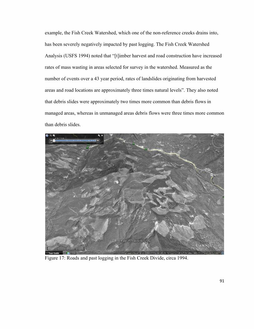
91  

 

example, the Fish Creek Watershed, which one of the non-reference creeks drains into,

has been severely negatively impacted by past logging. The Fish Creek Watershed

Analysis (USFS 1994) noted that “[t]imber harvest and road construction have increased

rates of mass wasting in areas selected for survey in the watershed. Measured as the

number of events over a 43 year period, rates of landslides originating from harvested

areas and road locations are approximately three times natural levels”. They also noted

that debris slides were approximately two times more common than debris flows in

managed areas, whereas in unmanaged areas debris flows were three times more common

than debris slides.

Figure 17: Roads and past logging in the Fish Creek Divide, circa 1994.

92  

 

Non-reference streams showed an increase in sediment-related water quality

parameters as well as in macroinvertebrates that have been associated with high sediment

conditions in other studies (gatherer-collectors, Chironomids, Oligochaetes, Dipterans,

and Turbellarians), suggesting that increased stream sediment levels are likely to be a

primary stressor in non-reference streams. It is worth noting, however, that reference

streams with high sediment levels continued to support macroinvertebrate assemblages

that were very dissimilar to non-reference streams, even those with very similar size and

streamflow, possibly suggesting that natural and anthropogenic sources of sediment

production may cause different responses in macroinvertebrate community compositions.

For example, Ora Creek had adjacent past burn and landslide activity, as well as the

highest turbidity and embeddedness of the reference creeks, and the lowest flows of

reference and non-reference creeks. Ora Creek also showed the closest association with

increasing percentage of silt/clay on the envfit overlay. Nevertheless, macroinvertebrate

assemblages in Ora Creek were more similar to other reference streams than to non-

reference streams in the NMDS ordination plot, possibly suggesting that adjacent

disturbance in this reference stream may have impacted stream biota differently

compared to anthropogenic disturbances in non-reference streams.

Greater annual precipitation in reference sites was associated with

macroinvertebrate assemblage distributional patterns, suggesting that climate as well as

natural and spatial variability between reference and non-reference sites may have been

influential. The three non-reference sites are spatially clustered together, and are

approximately 26 kilometers away from the three reference sites which are also spatially

93  

 

clustered together (i.e., located adjacent to each other). While both reference and non-

reference sites are in the Clackamas Basin, have similar and resistant geologies, and are

at very similar elevations, they are nevertheless spatially separate groupings of

subwatersheds which may exhibit natural variation in climactic patterns and other

environmental conditions such as instream fine sediment levels. Also, precipitation

events may have influenced turbidity, TDS, and conductivity in streams. However, with

the exception of a large precipitation event prior to fall sampling in Dog Creek, other

precipitation accumulation prior to sampling appeared relatively comparable between

non-reference and reference creeks. In addition, possible macroinvertebrates responses to

logging may be obscured by natural environmental gradients, particularly at large spatial

scales (Herlihy 2005, Sponseller et al. 2001). While this study examined a relatively

small spatial scale, Sponseller et al. (2001) found significant differences in

macroinvertebrate assemblages at the reach scale that were not evident at larger scales

such as the catchment scale.

The pattern of more similarity among macroinvertebrate assemblages in non-

reference streams shown on the NMDS ordination plot may be related to the land use

impacts in those watersheds. Literature suggests that homogenization of ecology and

biota may occur in response to anthropogenic stressors (Zhang et al. 2009). Water quality

parameters and environmental conditions in non-reference streams showed more

variability than in reference streams, possibly in response to anthropogenic disturbances.

While this study did not measure canopy structure or species composition, qualitative

observations suggest that these parameters were more complex and diverse at reference

94  

 

sites, including more herbaceous shrubs and plant and tree species diversity, which may

be partly responsible for the dissimilarity among macroinvertebrate assemblages in

reference sites. Homogenization of instream habitats due to past land use may also be

occurring in non-reference sites. For example, the Fish Creek Watershed Analysis (USFS

1994) states that by 1985, pools formed from large woody debris were at 11% of their

historic levels. Restoration efforts have concentrated on restoring large wood debris and

pool habitats, with these habitat features restored to approximately 25% of historic levels

at the time of the analysis. Recruitment for future large woody debris in riparian areas

was considered to be low, and at approximately half of historic levels (USFS 1994). It is

not clear what current levels are for large woody debris and pool habitats.

Recent Logging: NMDS Ordination and Correlations with Stream Sediment

Measures

The presence of recent logging within five years did not show any clear

associations with macroinvertebrate assemblage distributional patterns, suggesting that if

recent logging influenced stream biota, this influence was largely overshadowed by past

logging, roads, and other environmental conditions. Indications of increased fine

sediments have been found in relation to selective logging in certain sites in other studies

(Kreutzweiser et al. 2005, Miserendino and Masi 2010). In this study, limited evidence

exists to suggest that recent logging may be influencing water quality. In Canine and Dog

non-reference creeks, the upstream sites grouped together, as did downstream sites on the

NMDS ordination. Also, the percent of forest logged in the last five years in non-

reference catchments showed a moderate positive Pearson’s correlation coefficient with

95  

 

turbidity and embeddedness, as well as a moderate negative correlation with size of

streambed particles based on pebble counts, which may suggest a possible association

between recent management and water quality impacts. Canine and Dog Creeks (non-

reference) contained both high road densities and high percent of recent logging in their

watersheds, as well as similar significantly greater turbidity values compared to the

reference streams with most similar streamflows, and index scores suggesting the worst

water quality. Water quality responses to timber harvest may have complex temporal

patterns in these watersheds (Zhang et al. 2009). Possible impacts on streams associated

with current logging, if they exist, may manifest in different temporal and spatial scales

than were accounted for in this study, and would likely require long-term study and more

in-depth stream sampling to detect. Lecerf and Richardson (2010) noted that after logging

“the importance of abiotic and biotic changes in stream ecosystems varies nonlinearly

with the time elapsed since logging operations”.

Water Quality and Macroinvertebrates: Upstream vs. Downstream sites

Stream temperature was the only parameter for which a significant difference was

found in the magnitude of change from upstream to downstream of logging units in

reference vs. non-reference stream. Temperature increases may be related to adjacent

logging, though temperature data in this study this should be interpreted with caution

given that no continual probe equipment was used and temperature readings were only

collected during sample sessions. Selective logging has been shown to increase

temperature in other studies. Guenther et al. (2012) found increases in stream temperature

in relation to selective logging, and Johnson and Jones (2000) found increases in relation

96  

 

to patch cutting. Guenther et al. (2012) found increases in bed temperatures and in stream

daily maximum temperatures in relation to 50% removal of basal area in both upland and

riparian areas. Increases in daily maximum temperatures varied within the harvest area

from 1.6 to 3 degrees Celsius. Effects on stream temperature can vary depending on the

degree of logging within riparian buffers in both selective logging and in clearcuts.

Kiffney et al. (2003), when investigating varying buffer widths adjacent to clearcuts,

found that stream temperatures increased along a gradient of decreasing stream buffers

compared to controls, with a 3 °C increase in the 10 meter treatment and a 1.6 °C

increase in the 30 meter treatment. Decreasing buffer widths in their study corresponded

to increasing water mean temperatures in winter, spring, and summer, and maximum

temperatures in spring and summer. Increases in temperatures and alteration of

temperature regimes can directly affect macroinvertebrates, especially those that need

cold water for survival, as well as indirectly affect them through increased algal growth

and contributions to shifts towards autochthonous primary production. Other studies,

such as Lecerf and Richardson (2010), did not find any change in stream temperatures in

relation to selective logging.

Existing stream temperature data from the USFS for the Fish Creek watershed

creates a relevant context for viewing stream temperature data in non-reference sites in

this study. Multiple streams in the Fish Creek watershed have not meet water temperature

standards for core cold water habitat (USFS 1994, ODEQ accessed 2015) or for

designated spawning and rearing use (USFS accessed 2011) since at least 1999. In

addition, Fish Creek had higher average daily summer temperatures than any other

97  

 

stream surveyed within the Clackamas River subbasin, including temperatures repeatedly

reaching 75 degrees Fahrenheit (23.9 degrees Celsius), and the greatest diurnal

temperature fluctuations (USFS 1994). Seven day maximum temperatures continue to

exceed temperature standards in the most recent monitoring data available. For example,

2010 is the most recent year in which data is available (USFS accessed 2011), and

temperatures at the mouth of Fish Creek continue to exceed core cold water standards by

at least 3.5 degrees Celsius. Considering these observations of temperature data from the

USFS, stream temperature may be important to monitor in relation to selective logging

projects, particularly those that include logging within riparian buffers and in areas that

are already water quality limited or drain into water quality limited streams. The small

but significant increase in temperature found from upstream to downstream in non-

reference sites in this study should be interpreted with extreme caution because

temperature data were not continuous, and because the increase could be an artifact of

sampling time of day combined with small sample size. However, given the widespread

and continued exceedances of water temperature standards in the area, combined with

increases in temperature associated with selective logging in other studies possible

increases in temperature in relation to selective logging in the Clackamas at least merit

further investigation.

Contrary to my original hypotheses, no other significant difference in water

quality parameters or macroinvertebrate indices were detected in the magnitude of

change from upstream to downstream of logging units in reference vs. non-reference

sites. Several possible explanations exist for why impacts were not detected from

98  

 

upstream to downstream of recent selective harvest units: 1) Riparian buffers as well as

remaining trees left on the landscape in upland areas may have been sufficient to protect

water quality. 2) The “upstream” sites selected in this study failed to provide adequate

control points due to past and current land use activities that took place upstream of both

“upstream” and “downstream” study reaches. Land use activities and parameters which

may have impacted water quality above my upstream study reaches included the building

and use of temporary roads, high road densities, log haul, quarries, and (in one case)

current logging. Noise from these activities may have confounded or obscured impacts on

water quality due to the selective logging units. This study may have been unable to

detect impacts related to present logging due to difficulties in separating past logging and

chronic road impacts from current logging, especially since extensive current and past

impacts exist throughout the all non-reference watersheds. 3) Natural variability

obscured/confounded potential impacts on water quality. 4) Temporal responses to

logging, as discussed earlier in the discussion section, may complicate detection of

potential impacts. 5) The methodologies used in this study may have been insufficient to

detect changes in water quality from upstream to downstream. A larger sample size, in a

more spatially diverse set of subwatersheds, and with a gradient of logging intensity, may

have detected impacts.

Conclusion

The complex dynamics in stream ecosystems suggest that perhaps a more

precautionary approach to forest management may be necessary to protect listed and at-

risk species. For example, the recent study by Steele et al. (2014) found that subtle

99  

 

dynamics which may not have initially been recognized as harmful, such as diurnal

fluctuations in stream temperature- even stream temperatures that do not exceed 7-day

average maximum standards- may have negative impacts on salmonid survival (Steele et

al. 2014). In order to implement adaptive management, adhere to water quality standards,

and protect aquatic resources, it is important to determine what effects selective logging

in upland and riparian areas might have on stream temperature in particular and water

quality in general, and whether or not selective logging is achieving the desired

outcomes. However, a lack of sufficient data upon which to base land management

decisions and adaptive management strategies continues to be problematic. Monitoring

for in the Fish Creek watershed, for example, has not been implemented as extensively as

outlined in restoration plans, despite a long history of past impacts and a recognized

paucity of data. This study provides evidence that roads and past logging are influencing

water quality and macroinvertebrate assemblages and metrics. Recent logging was

correlated with sediment-related water quality parameters, and stream temperature may

have increased in relation to selective harvest units. These findings suggest that further

monitoring and research to determine possible effects of selective logging on water

quality and stream health should be prioritized, especially in watersheds with sensitive

and unique aquatic and riparian species.

100  

 

References

Adams, J. and Vaughan, M. (2007). Stream Bugs as Biomotiors: A Guide to Pacific Northwest Macroinvertebrate Monitoring. The Xerces Society.

Allan, J. (2004). Landscapes and riverscapes: the influence of land use on stream ecosystems. Annual Review of Ecology, Evolution, and Systematics, (35): 257-284.

Anderson, C. (2005). United States Geological Survey TWRI Book 9. Retrieved 2014 from <http://water.usgs.gov/owq/FieldManual/Chapter6/Section6.7_v2.1.pdf>.

Angradi, T. (1999). Fine sediment and macroinvertebrate assemblages in Appalachian streams: a field experiment with biomonitoring applications. Journal of North American Benthological Society, 18(1):49-66.

Bailey, R., Norris, R., Reynoldson, T. (2001). Taxonomic resolution of benthic macroinvertebrate communities in bioassessments. Journal of the North American Benthological Society, 20(2): 280-286.

Bain, M., and Stevenson, N. (1999). Aquatic habitat assessment: common methods. American Fisheries Society, Bethesda, MD. Retrieved 2014 from <http://imasd.fcien.edu.uy/difusion/educamb/docs/pdfs/aquaticmethods.pdf>.

Banks, J., Li, J., Herlihy, A. (2007). Influence of clearcut logging, flow duration, and season on emergent aquatic insects in headwater streams of the Central Oregon Coast Range. Journal of North American Benthological Society, 26(4): 620-632.

Bark (2012). In the forest: timber sale database and list of Clackamas Basin timber sales. Retrieved 2013 from <http://jbatch.geos.odin.pdx.edu/timbersales.html> and <http://www.bark-out.org/forest.php>.

Barbour, M., Gerritsen, J., Snyder, B., and Stribling, J. (1999). Rapid bioassessment protocols for use in streams and wadeable rivers: periphyton, benthic macroinvertebrates, and fish. Second edition. EPA-841-B-99-002. U.S. EPA, Office of Water, Washington, DC. Retrieved 2013 from <http://water.epa.gov/scitech/monitoring/rsl/bioassessment/index.cfm>.

Bauer, S. and Ralph, S. (2001). Strengthening the use of aquatic habitat indicators in clean water act programs. Fisheries, 26(6):14-25.

Bolstad, P. and Swank, W. (2007). Cumulative impacts of landuse on water quality in a southern Appalachian watershed. Journal of American Waters Association, 33(3): 519-533.

101  

 

Bryce, S., Lomnicky, G., and Kaufmann, P. (2010), Protecting sediment-sensitive aquatic species in mountain streams through the application of biologically based streambed sediment criteria. Journal of the North American Benthological Society, 29(2):657-672.

Cederholm C., Reid L., Salo E. (1980). Cumulative effects of logging road sediment on salmonid populations in Clearwater River, Jefferson County, Washington. College of Fisheries, University of Seattle, Washington. Retrieved 2014 from <http://www.fs.fed.us/psw/publications/reid/Cederholm.pdf>.

Cover, M., May, C., Dietrich, W., Resh, V. (2008). Quantitative linkages among sediment supply, streambed fine sediment, and benthic macroinvertebrates in northern California streams. Journal of the North American Benthological Society, 27(1):135-149.

Croke, J. and Hairsine, P. (2006). Sediment delivery in managed forests: a review. Environmental Review, (14): 59-87.

Daniels, J. (2001). Timber processing capacity in Oregon: why mills still matter. Lecture and Powerpoint at Portland State University. United States Department of Agriculture and the Bureau of Business and Economic Research.

Decker v. Northwest Environmental Defense Center (2013), 568 U.S. Retrieved 2015 from <http://www.supremecourt.gov/opinions/12pdf/11-338_kifl.pdf>.

Dyrness, C., (1967). Mass soil movements in the H.J. Andrews experimental forest. Retrieved 2014 from <http://hdl.handle.net/2027/umn.31951d02995036k>.

Edwards, T., and Glysson, G. (1999). Techniques for water resource investigations of the United States Geological Society, Book 3 Applications of Hydraulics, Chapter C2: Field methods for measurements of fluvial sediment. United States Geological Society. Retrieved 2014 from <http://pubs.usgs.gov/twri/twri3-c2/pdf/twri_3-C2_c.pdf>.

Ellison, C., Kiesling, R., and Fallon, J. (2010). Correlating streamflow, turbidity, and suspended-sediment concentration in Minnesota’s Wild Rice River. United States Geological Survey, Second Joint Federal Interagency Conference, Las Vegas, NV. Retrieved 2014 from <http://acwi.gov/sos/pubs/2ndJFIC/Contents/8B_Ellison_12_03_09_paper.pdf>.

Flaspohler, D., Fisher, C., Huckins, C., Bub, B., and Van Dusen, P. (2002). Temporal patterns in qquatic and avian communities following selective logging in the Upper Great Lakes Region. Forest Science, 48(2):339–349.

102  

 

Galloway, J., Evans, D., and Green, R. (2005). Comparability of suspended-sediment concentrations and total suspended-solids data for two sites on the L’Anguille River, Arkansas, 2001 to 2003. Scientific Investigations Report 2005-5193. United States Geological Survey. Retrieved 2014 from <http://pubs.usgs.gov/sir/2005/5193/SIR2005-5193.pdf>.

Gravelle, J., Link, T., Broglio, J., and Braatne, J. (2009). Effects of timber harvest on aquatic macroinvertebrate community composition in a northern Idaho watershed. Society of American Foresters, 55(4): 352-366.

Gray, J., Glysson, G., Turcios, L., and Schwarz, G. (2000), Comparability of total suspended solids and suspended-sediment concentration data: U.S. Geological Survey Water-Resources Investigations Report 00–4191, 14. Retrieved 2014 from <http://water.usgs.gov/osw/pubs/WRIR00-4191.pdf>.

Gray, J., Laronne, J., and Marr, J. (2010). Bedload-surrogate monitoring technologies. United States Geological Survey (USGS). Reston, Virginia. Retrieved 2012 from <http://pubs.usgs.gov/sir/2010/5091/pdf/sir2010-5091.pdf>.

Guenther, S., Gomi, T., and Moore, R. (2012). Stream and bed temperature variability in a coastal headwater catchment: influences of surface-subsurface interactions and partial-retention forest harvesting. Hydrological Processes, 28: 1238–1249.

Guthrie, R. (2001). The effects of logging on frequency and distribution of landslides in three watersheds on Vancouver Island, British Columbia. Geomorphology 43(3-4): 273-292.

Guy, H. (1969). Techniques of water resources investigations for the United States Geological Survey: Chapter C1: Laboratory theory and methods for sediment analysis. United States Geological Survey. Retrieved 2014 from <http://pubs.usgs.gov/twri/twri5c1/pdf/twri_5-C1_a.pdf>.

Hach Co. (1999). Portable Turbidimeter Model 2100P Instrument and Procedure Manual. Catalog number 46500-88.

Haggarty, S., Batzer, D., and Jackson, C. (2003). Macroinvertebrate response to logging in coastal headwater streams in Washington, USA. Canadian Journal of Fisheries and Aquatic Sciences, 61(4): 529-537.

Harr, D. and Coffin, B. (1992). Influence of timber harvest on rain-on-snow runoff: a mechanism for cumulative watershed effects. Interdisciplinary approaches in hydrology and hydrogeology. American Institute of Hydrology: 455-469.

103  

 

Henley, W., Patterson, M., Neves, R., and Lemly, D. (2000). Effects of sedimentation and turbidity on lotic food webs: a concise review for natural resource managers. Reviews in Fisheries Science, 8(2): 125–139.

Herlihy, A., Gerth, W., Li, J., and Banks, J. (2005). Macroinvertebrate community response to natural and forest harvest gradients in western Oregon headwater streams. Freshwater Biology, (50): 905-919.

Hewlett, R. (2000). Implications of taxonomic resolution and sample habitat for stream classification at a broad geographic scale. Journal of North American Benthological Society, 19(2): 352–361.

Hicks, B., Beschta, R., and Harr, D. (1991). Long-term changes in streamflow following logging in western Oregon and associated fisheries implications. Water Resources Bulletin, (27):2.

Hilsenhoff, W. (1988). Rapid field assessment of organic pollution with a family-level biotic index. Journal of the North American Benthological Society, (7): 65-68.

Hlass, L., Fisher, W., and Turton, D. (1998). Use of the index of Biotic Integrity to assess water quality in forested streams of the Ouachita Mountains ecoregion, Arkansas. Journal of Freshwater Ecology, 13(2): 181-192.

Idaho Department of Environmental Quality (IDEQ). (2003). Guide for selection of sediment targets for use in Idaho TMDLs. Retrieved from <http://www.deq.state.id.us/WATER/ data_reports/surface_ water/monitoring/sediment_targets_guide.pdf>.

Jones, J. (2000). Hydrologic processes and peak discharge response to forest removal, regrowth, and roads in 10 small experimental basins, western Cascades, Oregon. Water Resources Research, 36(9): 2621-2642.

Jones, J. and Grant, G. (1996). Peak flow responses to clear-cutting and roads in small and large basins, western Cascades, Oregon. Water Resources Research, 32(4): 959-974.

Johnson, S., and Jones, J. (2000). Stream temperature responses to forest harvest and debris flows in western Cascades, Oregon. Canadian Journal of Fisheries and Aquatic Sciences, 57(2): 30–39.

Johnson, L., Richards, C., Host, G., and Arthur, J. (2003). Landscape influences on water chemistry in Midwestern stream ecosystems. Freshwater Biology, 37 (1): 193-208.

104  

 

Kiffney, P., Richardson, J., and Bull, J. (2003). Responses of periphyton and insects to experimental manipulation of riparian buffer width along forest streams. Journal of Applied Ecology, (40) 1060–1076.

Klemm, D., Lewis, P., Fulk, F., and Lazorchak, J. (1990). Macroinvertebrate field and laboratory methods for evaluating the biological integrity of surface waters. USEPA. Retrieved 2012 from <http://www.epa.gov/bioiweb1/pdf/EPA600490030MacroinvertebrateFieldandLaboratoryMethodsforEvalutingtheBiologicalIntegrityofSurfaceWaters.pdf>.

Kreutzweiser , D., Capell, S., and Good, K. (2005). Macroinvertebrate community responses to selection logging in riparian and upland areas of headwater catchments in a northern hardwood forest. Journal of the North American Benthological Society, 24(1):208-222.

Kreutzweiser, D. and Capell, S. (2001). Fine sediment deposition in streams after selective forest harvesting without riparian buffers. Canadian Journal of Forest Research, v. 31 p. 2134-2142.

Lazorchak, J., Klemm, D., and Peck, D. (1998). Environmental monitoring and assessment program – surface waters: field operations and methods for measuring the ecological condition of wadeable streams. US Environmental Protection Agency. Retrieved 2012 from <http://www.epa.gov/bioiweb1/pdf/EPA-620-R-94-004FFieldOperationsandMethodsforMeasuringtheEcologicalConditionofWadeableStreams.pdf>.

Lecerf, A. and Richardson, J. (2010). Litter decomposition can detect effects of high and moderate levels of forest disturbance on stream condition. Forest Ecology and Management, 259 (2010) 2433–2443.

Lenat, D. and Resh, V. (2001). The benefits of genus- and species-level identifications. Journal of the North American Benthological Society, (20): 2, 287-298.

Lewis, J., Mori, S., Keppeler, E., and Ziemer, R. (2001). Impacts of logging on storm peak flows, flow volumes and suspended sediment loads in Casper Creek, California. Land use and watersheds: human influence on hydrology and geomorphology in urban and forest areas. American Geophysical Union: 85-126.

Lewis, J. (2003). Turbidity controlled sampling for suspended sediment load estimation. United States Department of Agriculture, Forest Service, Pacific Southwest Research Station, Ca, USA. Retrieved 2013 from <http://www.fs.fed.us/psw/publications/4351/Lewis2003b.pdf>.

105  

 

Lewis, J. and Eads, R. (2009). Implementation guide for turbidity threshold sampling: principles, procedures, and analysis. USFS Pacific Southwest Research Station, General Technical Report PSW-GTR-212. Retrieved 2013 from <http://www.fs.fed.us.proxy.lib.pdx.edu/psw/publications/4351/Lewis2009.pdf>.

Mandeville, S. (2002). Benthic macroinvertebrates in freshwaters- taxa tolerance values, metrics, and protocols. Soil & Water Conservation Society of Metro Halifax. Retrieved 2014 from <http://lakes.chebucto.org/H-1/tolerance.pdf>.

Merritt, R. and Cummins, B. (2008). Introduction to the aquatic insects of North America. Fourth edition, Kendall/Hunt Publishing Co., Dubuque, Iowa.

Miserendino, L. and Masi, C. (2010). The effects of land use on environmental features and functional organization of macroinvertebrate communities in Patagonian low order streams. Ecological Indicators, 10(2): 311-319.

Montgomery, D., Schmidt, K., Greenberg, H., and Dietrich, W. (2000). Forest clearing and regional landsliding. Geological Society of America, (28): 311-314.

Moore, D. and Wondzell, S. (2005), Physical hydrology and the effects of forest harvesting in the Pacific Northwest: A review. Journal of the American Waters Association, 41(4): 763-784.

Nietch, C., Borst, M., and Schubauer-Berigan, J. (2005). Risk management of sediment stress: a framework for sediment risk management research. Environmental Management, (36):175–194.

National Oceanic and Atmospheric Administration (NOAA) 1996. Coastal salmon conservation: working guidance for comprehensive salmon restoration initiatives on the Pacific coast. Retrieved 2014 from <http://www.krisweb.com/biblio/gen_noaa_nmfs_1996_salmonconservation.pdf>.

Northwest Environmental Defense Center vs. Brown (2010). Ninth Circuit Court. Retrieved 2015 from <http://wflc.org/cases/docket/nedcvbrown>.

Olsen, D., Roper, B., Kershner, J., Henderson, R., and Archer, E. (2005). Sources of Variability in conducting pebble counts: their potential influence on the results of stream monitoring programs. Journal of American Water Resources Association, 41(5):1225-1236.

Oregon Department of Fish and Wildlife (ODFW). (2010). Willamette River Fish Recovery. Educational web resource. Retrieved 2014 from <http://www.dfw.state.or.us/fish/CRP/docs/upper_willamette/FAQ.pdf>.

106  

 

Oregon Department of Water Quality (ODEQ). (2006). Willamette Basin TMDL: Clackamas Subbasin. Retrieved 2015 from <http://www.deq.state.or.us/wq/tmdls/docs/willamettebasin/willamette/chpt6clackamas.pdf>.

Oregon Department of Water Quality (ODEQ). (Accessed 2013). Water quality standards- beneficial uses tables and figures. Retrieved 2014 from <http://www.deq.state.or.us/wq/rules/div041tblsfigs.htm>.

Oregon Department of Water Quality (ODEQ). (Accessed 2015). Oregon Administrative Rules (OAR) 340-041, Retrieved 2015 from <http://arcweb.sos.state.or.us/pages/rules/oars_300/oar_340/340_041.html>.

Oregon Department of Water Quality (ODEQ). (Accessed 2015). Water quality assessment database. Retrieved 2015 from <http://www.deq.state.or.us/wq/assessment/rpt2010/results.asp>.

Packman, J., Comings K., and Booth, D. (2000). Using turbidity to determine total suspended solids in urbanizing streams in the Puget lowlands. The Center for Urban Water Resources Management at the University of Washington, Seattle, Washington.

Pacific Northwest Ecosystem Research Consortium. Accessed (2013). GIS geologic data. Retrieved 2012 from <http://oregonstate.edu/dept/pnw-erc/>.

Piccolo, J., and Wipfli, M. (2002). Does red alder (Alnus rubra) in upland riparian forests elevate macroinvertebrate and detritus export from headwater streams to downstream habitats in southeastern Alaska? Canadian Journal of Fisheries and Aquatic Sciences, (59): 2002.

Pollock, M., Beechie, T., and Imake, H. (2012). Using reference conditions in ecosystem restoration: an example for riparian conifer forests in the Pacific Northwest. ESA journal, 3(11): 98.

Pollock, M. and Beechie, T. (2014). Does riparian forest thinning enhance forest biodiversity? The ecological importance of downed wood. Journal of American Waters Resource Association (JAWRA), 50(3): 543-559.

Progar, R. and Moldenke, A. (2009). Aquatic insect emergence from headwater streams flowing through regeneration and mature forests in Western Oregon, Journal of Freshwater Ecology, (24):1, 53-66.

107  

 

Rasmussen, P., Gray, J., Glyyson, D., and Ziegler, A., (2011). Guidelines and procedures for computing time-series suspended-sediment concentrations and loads from in-stream turbidity-sensor and streamflow data. U.S. Geological Survey Techniques and Methods, book 3, chap. C4. Retrieved 2012 from <http://pubs.usgs.gov/tm/tm3c4/pdf/TM3C4.pdf>.

Reid, D., Quinn, J., and Wright-Stow, A. (2010). Responses of stream macroinvertebrate communities to progressive forest harvesting: Influences of harvest intensity, stream size and riparian buffers. Forest Ecology and Management, 260(10):< 1804–1815.

Relyea, C., Minshall G., and Danehy. R. (2000). Stream insects as bioindicators of fine sediment. Watershed Management 2000 Conference. Water Environment Federation, Alexandria, VA. Retrieved 2014 from <https://www.deq.idaho.gov/media/525820-Stream_Insects_Bioindicators_Fine_Sediment_Relyea_2000.pdf>.

Relyea, C., Minshall G., and Danehy, R. (2012). Development and validation of a fine sediment biotic index. Environmental Management, (49):242–252

Richardson, J. and Danehy, R. (2005). A synthesis of the ecology of headwater streams and their riparian zones in temperate forests. Forest Science, 53(2) 2007.

Salminen, E. (2005). Clackamas Basin Watershed summary overview. Watershed Professionals Network, prepared for Clackamas River Basin Council, Clackamas, Oregon.

Scott, M., Helfman, M., McTammany, M., Benfield, F., and Bolstad, P. (2007). Multiscale influences on physical and chemical stream conditions across blue ridge landscapes. Journal of American Water Resources Association. 38(5): 1379-1392.

Sigma-Adrich Supply Co. 2012. Whatman glass microfiber filters, binder free, grade GF/C 24 mm. Retrieved 2012 from <http://www.sigmaaldrich.com/catalog/product/aldrich/Z242330?lang=en&region=US>.

Smith, B., Davies, P., and Munks, S. (2009). Changes in macroinvertebrate communities in upper catchment streams across a gradient of catchment forest operation history. Forest Ecology and Management, (257): 2166-2174.

Sponseller, R., Benfield, E., and Valett, H. (2001). Relationship between land use, spatial scale, and stream macroinvertebrate communities. Freshwater Biology, (46): 1409-1424.

108  

 

Stark, J., Boothroyd, I.. Harding, J., Maxted, J., and Scarsbrook, M. (2001). Protocols for sampling macroinvertebrates in wadeable streams. New Zealand Macroinvertebrate Working Group Report No. 1. Prepared for the Ministry for the Environment. Sustainable Management Fund Project (5103): 57.

Steele, A., Beckman, B.; and Oliver, M. (2014). Stream temperature variability: why it matters to salmon. Science findings 163. Portland, OR: US Department of Agriculture, Forest Service, Pacific Northwest Research Station. Science findings (163): 6.

Stone, M. and Wallace, B. (1998). Long-term recovery of a mountain stream from clearcut logging: the effects of forest succession on benthic invertebrate community structure. Freshwater Biology, (39):151-169.

Swanson, F. and Swanston, D. (1977). Complex mass movement terrains in the western Cascades Range, Oregon. Geological Society of America, (3).

Tague, C. and Grant, G. (2004). A geological framework for interpreting the low-flow regimes of Cascade streams, Willamette River Basin, Oregon. Water Resources Research, (40): W04303.

Taylor, B. (1999). Salmon and steelhead runs and related events of the Clackamas River Basin – a historical percpective. Prepared for Portland General Electric. Retrieved 2013 from <https://www.portlandgeneral.com/community_environment/initiatives/protecting_fish/clackamas_river/docs/clackamas_river_history_full.pdf>.

Troendle, C. and Olsen, W. (1993). Potential Effects of Timber Harvest and Water Management on Streamflow Dynamics and Sediment Transport. In: Sustainable Ecological Systems Proceedings. USDA Forest Service, Rocky Mountain Forest and Range Experiment Station GTR RM-247, Fort Collins, Colorado, pp. 34-41.

Ulrich, M. (2002). The advantage of continuous turbidity monitoring: a lesson from the North Santiam River Basin, Oregon; 1998-2000. Turbidity and other sediment surrogates workshop, April 30 – May 2, 2002, Reno, Nevada. US Geological Survey. Retrieved 2013 from <http://water.usgs.gov/osw/techniques/TSS/uhrich1.pdf>.

United States Environmental Protection Agency (USEPA). (2002). Using Biological Data as Indicators of Water Quality. Retrieved 2013 from <http://www.epa.gov/owow/monitoring/calm/calm_ch5.pdf>.

109  

 

United States Environmental Protection Agency (USEPA). (2006). Framework for Developing Suspended and Bedded Sediments (SABS) Water Quality Criteria. Retrieved 2013 from <http://cfpub.epa.gov/ncea/cfm/recordisplay.cfm?deid=164423#Download>.

United States Environmental Protection Agency (USEPA). (2007). The wadeable streams assessment: a collaborative survey of the nation’s streams. Fact sheet. Retrieved 2012 from <http://water.epa.gov/type/rsl/monitoring/upload/2007_10_25_monitoring_wsa_factsheet_10_25_06.pdf>.

United States Forest Service (USFS). (1979). Soil Resource Inventory, Mt. Hood National Forest. United States Department of Agriculture. Retrieved 2013 from <http://www.fs.fed.us/r6/data-library/gis/mthood/>.

United States Forest Service (USFS). (1993). Clackamas National Wild and Scenic River and State Scenic Byway, Environmental Assessment and Management Plan. United States Department of Agriculture, Pacific Northwest Region. Retrieved 2014 from <http://www.fs.usda.gov/Internet/FSE_DOCUMENTS/fsbdev3_036590.pdf>.

United States Forest Service (USFS). (1994). Fish Creek Watershed Analysis. United States Department of Agriculture. Retrieved 2014 from <http://www.fs.usda.gov/Internet/FSE_DOCUMENTS/fsbdev3_036587.pdf >.

United States Forest Service (USFS) (2004). Forests of western Oregon, an overview. United States Department of Agriculture. Retrieved 2013 from <http://www.fs.fed.us/pnw/publications/gtr525/gtr525a.pdf>.

United States Forest Service (USFS). (2006). 2007 Plantation Thin Biological Assessment. United States Department of Agriculture. Retrieved 2014 from <http://www.bark-out.org/sites/default/files/bark-docs/2007_Thin_Final_Fish_BA.htm>.

United States Forest Service (USFS). (2006). Preliminary Assessment 2007 Plantation Thinning. United States Department of Agriculture. Retrieved 2014 from <http://www.bark-out.org/sites/default/files/bark-docs/2007_preliminary_assessment.pdf

United States Forest Service (USFS). (2010). Mt. Hood National Forest annual monitoring report. United States Department of Agriculture. Retrieved 2013 from <http://www.fs.usda.gov/main/mthood/landmanagement/planning>

110  

 

United States Forest Service (USFS). (Accessed 2011). Unpublished GIS data for timber sales and roads, obtained by FOIA request.

United States Forest Service (USFS). (2012). National Best Management Practices for water quality management on national forest system lands. United States Department of Agriculture. Retrieved 2012 from <http://www.fs.fed.us/biology/resources/pubs/watershed/FS_National_Core_BMPs_April2012.pdf>.

United States Forest Service (USFS). (2012). Forest Service schedule of proposed actions for Mt. Hood National Forest. United States Department of Agriculture. Retrieved 2012 from <http://www.fs.fed.us/sopa/forest-level.php?110606>.

United States Forest Service (USFS). (Accessed 2012). Mt. Hood National Forest data library, Geographic Information Services. Retrieved 2013 from <http://www.fs.fed.us/r6/data-library/gis/mthood/index.shtml>.

US Fish and Wildlife Service. (2013). Bull trout reintroduction project. <http://www.fws.gov/oregonfwo/Species/Data/BullTrout/ReintroductionProject.asp>.

United States Geological Survey (USGS). (1998). USGS WRD sediment laboratory chiefs workshop. Retrieved 2012 from <http://water.usgs.gov/osw/techniques/USGSsedlab98.html>.

United States Geological Survey (USGS). (2000). Office of water quality technical memorandum no. 2001.03. Retrieved 2013 from <http://water.usgs.gov/admin/memo/SW/TSS.0103.html>.

United States Geological Survey (USGS). (Accessed 2012). Geologic units in Clackamas County. Retrieved 2012 from <http://mrdata.usgs.gov/geology/state/fips-unit.php?code=f41005>.

United States Geological Survey (USGS). (Accessed 2012). Surface water information. Retrieved 2012 from <http://water.usgs.gov/osw/data.html>.

United States Geological Survey (USGS). (Accessed 2013). Streamstats. Retrieved 2013 from <http://streamstatsags.cr.usgs.gov/or_ss/default.aspx?stabbr=or&dt=1365800898467>.

Waters, T. (1995). Sediment in streams: sources, biological effects and control. American Fisheries Society, Bethesda, Maryland.

111  

 

Webster, J., Golladay, S., Benfield, E., Meyer, J., Swank, W., and Wallace, J. (1992). Catchment disturbance and stream response: an overview of stream research at Coweeta Hydrologic Laboratory. River Conservation and Management.

Wemple, B., Jones, J., and Grant, G. (1996). Channel network extension by logging roads in two basins, western Cascades, Oregon. Water Resources Bulletin, 32(6).

Wemple, B., Swanson, F., and Jones, J. (2000). Forest roads and geomorphic process interactions, Cascade Range, Oregon. Earth Surface Landforms and Processes, (26): 191-204.

Whitman, M., Moran, E., and Ourso, R. (2003). Photographic techniques for characterizing streambed particle sizes. American Fisheries Society, (132): 605-610.

Willacker, J., Sobczak, W., and Colburn, E. (2009). Stream macroinvertebrate communities in paired hemlock and deciduous watersheds. Northeastern naturalist, 16(1):101-112.

Wood, P. and Armitage P. (1997). Biological effects of fine sediment in the lotic environment. Environmental Management, 21(2): 203–217.

Zhang, Y., Richardson, J., and Pinto, X. (2009). Catchment-scale effects of forestry practices on benthic invertebrate communities in Pacific coastal streams. Journal of Applied Ecology, (46): 1292-1303.

Zweig, L. and Rabeni, C. (2001). Biomonitoring for deposited sediment using macroinverterbrate benthic invertebrates: a test on four Missouri streams. Journal of North American Benthological Society, (20)4:643-657.