Edinburgh Research Explorer

Multiscale Topological Trajectory Classification with PersistentHomology

Citation for published version: pokorny, F, Hawasly, M & Ramamoorthy, S 2014, Multiscale Topological Trajectory Classification withPersistent Homology. in Proceedings of Robotics: Science and Systems X 2014. Berkeley, USA.

Link:Link to publication record in Edinburgh Research Explorer

Document Version:Publisher's PDF, also known as Version of record

Published In:Proceedings of Robotics: Science and Systems X 2014

General rightsCopyright for the publications made accessible via the Edinburgh Research Explorer is retained by the author(s)and / or other copyright owners and it is a condition of accessing these publications that users recognise andabide by the legal requirements associated with these rights.

Take down policyThe University of Edinburgh has made every reasonable effort to ensure that Edinburgh Research Explorercontent complies with UK legislation. If you believe that the public display of this file breaches copyright pleasecontact openaccess@ed.ac.uk providing details, and we will remove access to the work immediately andinvestigate your claim.

Download date: 17. Jun. 2018

Multiscale Topological Trajectory Classificationwith Persistent Homology

Florian T. PokornyCentre for Autonomous Systems, CSC

KTH Royal Institute of Technology, Sweden

Majd HawaslyIPAB, School of Informatics

University of Edinburgh, UK

Subramanian RamamoorthyIPAB, School of Informatics

University of Edinburgh, UK

Abstract—Topological approaches to studying equivalenceclasses of trajectories in a configuration space have recentlyreceived attention in robotics since they allow a robot to reasonabout trajectories at a high level of abstraction. While recentwork has approached the problem of topological motion planningunder the assumption that the configuration space and obsta-cles within it are explicitly described in a noise-free manner,we focus on trajectory classification and present a sampling-based approach which can handle noise, which is applicableto general configuration spaces and which relies only on theavailability of collision free samples. Unlike previous sampling-based approaches in robotics which use graphs to captureinformation about the path-connectedness of a configurationspace, we construct a multiscale approximation of neighbor-hoods of the collision free configurations based on filtrations ofsimplicial complexes. Our approach thereby extracts additionalhomological information which is essential for a topologicaltrajectory classification. By computing a basis for the firstpersistent homology groups, we obtain a multiscale classificationalgorithm for trajectories in configuration spaces of arbitrarydimension. We furthermore show how an augmented filtrationof simplicial complexes based on a cost function can be definedto incorporate additional constraints. We present an evaluationof our approach in 2, 3, 4 and 6 dimensional configuration spacesin simulation and using a Baxter robot.

I. INTRODUCTION

The problem of determining a continuous path γ : [0, 1]→Cf between two points in the collision free subset Cf of someconfiguration space C ⊆ Rd is an important classical motionplanning problem. Since, in realistic robotics applications,an explicit description of Cf is often not available, popularalgorithms such as Rapidly-exploring Random Trees (RRT)and Probabilistic Roadmaps (PRM) [25, 24, 20] are basedon the idea of utilizing a set of random samples X ⊂ Cfto construct a graph Γ with vertices in Cf and where edgescorrespond to local paths which can be determined by a localpath planner. The graph Γ can then be used to efficientlycarry out motion planning. If Cf is a tame space, Γ, forsufficiently large X , provides an approximation of Cf whichallows us to answer basic questions about the path-connectivityof Cf . However, Γ does typically not capture higher orderhomological information.

In this paper, we propose a novel approach based onfiltrations F = {Fr : r > 0} of simplicial complexes definedin terms of random samples X ⊂ Cf . From such filtrations,we then extract higher-order topological information for thepurpose of understanding and classifying equivalence classes

of trajectories in Cf . Given a sufficiently good approximationof Cf by Fr, our approach yields a finite set of equivalenceclasses with the property that no trajectory belonging toone equivalence class can be continuously deformed to anytrajectory in any of the other equivalence classes. Our filtrationF is based on Delaunay-Cech complexes which depend on ascale parameter r and which have very recently been proven[3] to provide a homotopy-equivalent reconstruction of thespace Xr =

⋃x∈X Br(x) [3], where Br(x) = {y ∈ Rd : ‖x−

y‖ 6 r}. Our work utilizes persistent homology [15, 11, 16]which generalizes classical homology groups to a multiscalesetting – meaning that we are able to compute topologicalinformation about the analogue Fr of Γ for all scales r > 0simultaneously without having to choose a particular scaleupfront. Additionally, the 1-skeleton F1

r ⊆ Fr is a graphwhich can be used for path-planning. When a cost functionc : Cf → R is defined, we furthermore study the space ofpaths in Mr,λ = Xr ∩ c−1(−∞, λ] and show how resultingpath classes can be obtained. We evaluate our approach in 2,3, 4, and 6 dimensions in simulation and using a Baxter robot.

II. MOTIVATION AND RELATED WORK

For a robot to reason efficiently about trajectories withinits own free configuration space Cf , or about the motions ofother human or robot agents in its environment, a suitablepartitioning of continuously varying families of trajectoriesinto a discrete set of equivalence classes is desirable.

Clustering trajectories is difficult in general since trajecto-ries can have varying length and are not immediately rep-resentable as vectors in a vector space of fixed dimension asrequired by commonly used algorithms. Several approaches tothe classification of trajectories, as reviewed in [33], are basedon various approaches to measuring the dissimilarity betweentrajectories, such as the Hausdorff distance, edit distances anddynamic time warping. For the purpose of activity analysis, thework of [29] reviews trajectory clustering approaches based onvarious clustering algorithms and distance measures.

In robotics, the knowledge of classes of trajectories is bene-ficial for example in the learning by demonstration framework[8] where movement primitives of a robot’s behavior areconstructed from initial trajectory demonstrations provided bya human teacher. Equivalence classes of robot trajectories canfurthermore be useful in order to reason about alternativetrajectories when a subset of trajectories becomes invalid due

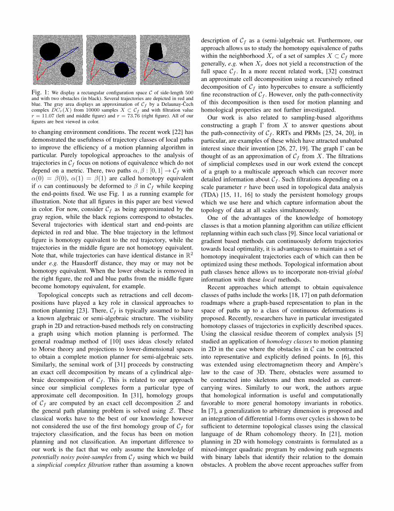
Fig. 1: We display a rectangular configuration space C of side-length 500and with two obstacles (in black). Several trajectories are depicted in red andblue. The gray area displays an approximation of Cf by a Delaunay-Cechcomplex DCr(X) from 10000 samples X ⊂ Cf and with filtration valuer = 11.07 (left and middle figure) and r = 73.76 (right figure). All of ourfigures are best viewed in color.

to changing environment conditions. The recent work [22] hasdemonstrated the usefulness of trajectory classes of local pathsto improve the efficiency of a motion planning algorithm inparticular. Purely topological approaches to the analysis oftrajectories in Cf focus on notions of equivalence which do notdepend on a metric. There, two paths α, β : [0, 1]→ Cf withα(0) = β(0), α(1) = β(1) are called homotopy equivalentif α can continuously be deformed to β in Cf while keepingthe end-points fixed. We use Fig. 1 as a running example forillustration. Note that all figures in this paper are best viewedin color. For now, consider Cf as being approximated by thegray region, while the black regions correspond to obstacles.Several trajectories with identical start and end-points aredepicted in red and blue. The blue trajectory in the leftmostfigure is homotopy equivalent to the red trajectory, while thetrajectories in the middle figure are not homotopy equivalent.Note that, while trajectories can have identical distance in R2

under e.g. the Hausdorff distance, they may or may not behomotopy equivalent. When the lower obstacle is removed inthe right figure, the red and blue paths from the middle figurebecome homotopy equivalent, for example.

Topological concepts such as retractions and cell decom-positions have played a key role in classical approaches tomotion planning [23]. There, Cf is typically assumed to havea known algebraic or semi-algebraic structure. The visibilitygraph in 2D and retraction-based methods rely on constructinga graph using which motion planning is performed. Thegeneral roadmap method of [10] uses ideas closely relatedto Morse theory and projections to lower-dimensional spacesto obtain a complete motion planner for semi-algebraic sets.Similarly, the seminal work of [31] proceeds by constructingan exact cell decomposition by means of a cylindrical alge-braic decomposition of Cf . This is related to our approachsince our simplicial complexes form a particular type ofapproximate cell decomposition. In [31], homology groupsof Cf are computed by an exact cell decomposition Z andthe general path planning problem is solved using Z . Theseclassical works have to the best of our knowledge howevernot considered the use of the first homology group of Cf fortrajectory classification, and the focus has been on motionplanning and not classification. An important difference toour work is the fact that we only assume the knowledge ofpotentially noisy point-samples from Cf using which we builda simplicial complex filtration rather than assuming a known

description of Cf as a (semi-)algebraic set. Furthermore, ourapproach allows us to study the homotopy equivalence of pathswithin the neighborhood Xr of a set of samples X ⊂ Cf moregenerally, e.g. when Xr does not yield a reconstruction of thefull space Cf . In a more recent related work, [32] constructan approximate cell decomposition using a recursively refineddecomposition of Cf into hypercubes to ensure a sufficientlyfine reconstruction of Cf . However, only the path-connectivityof this decomposition is then used for motion planning andhomological properties are not further investigated.

Our work is also related to sampling-based algorithmsconstructing a graph Γ from X to answer questions aboutthe path-connectivity of Cf . RRTs and PRMs [25, 24, 20], inparticular, are examples of these which have attracted unabatedinterest since their invention [26, 27, 19]. The graph Γ can bethought of as an approximation of Cf from X . The filtrationsof simplicial complexes used in our work extend the conceptof a graph to a multiscale approach which can recover moredetailed information about Cf . Such filtrations depending on ascale parameter r have been used in topological data analysis(TDA) [15, 11, 16] to study the persistent homology groupswhich we use here and which capture information about thetopology of data at all scales simultaneously.

One of the advantages of the knowledge of homotopyclasses is that a motion planning algorithm can utilize efficientreplanning within each such class [9]. Since local variational orgradient based methods can continuously deform trajectoriestowards local optimality, it is advantageous to maintain a set ofhomotopy inequivalent trajectories each of which can then beoptimized using these methods. Topological information aboutpath classes hence allows us to incorporate non-trivial globalinformation with these local methods.

Recent approaches which attempt to obtain equivalenceclasses of paths include the works [18, 17] on path deformationroadmaps where a graph-based representation to plan in thespace of paths up to a class of continuous deformations isproposed. Recently, researchers have in particular investigatedhomotopy classes of trajectories in explicitly described spaces.Using the classical residue theorem of complex analysis [5]studied an application of homology classes to motion planningin 2D in the case where the obstacles in C can be contractedinto representative and explicitly defined points. In [6], thiswas extended using electromagnetism theory and Ampere’slaw to the case of 3D. There, obstacles were assumed tobe contracted into skeletons and then modeled as current-carrying wires. Similarly to our work, the authors arguethat homological information is useful and computationallyfavorable to more general homotopy invariants in robotics.In [7], a generalization to arbitrary dimension is proposed andan integration of differential 1-forms over cycles is shown to besufficient to determine topological classes using the classicallanguage of de Rham cohomology theory. In [21], motionplanning in 2D with homology constraints is formulated as amixed-integer quadratic program by endowing path segmentswith binary labels that identify their relation to the domainobstacles. A problem the above recent approaches suffer from

is that they require an explicit description of the obstaclesin the configuration space, e.g. in 2D as unions shapes eachof which is contractible to a geometrically specified pointp ∈ C − Cf . In many cases, such information is howevernot easily available for real robotic systems or too expensiveto compute. We instead propose a data-driven, sampling-based approach to building a representation of Cf from whichtopological information about trajectories can be extracted.

III. THEORETICAL BACKGROUND

Filtrations and persistent homology provide a key tool todetermine multiscale topological properties. We review someconcepts from topological data analysis [15, 16].

A. Delaunay-Cech Complexes

A (abstract) k-simplex σ is a set of k+ 1 elements, and wecall k the dimension of σ. A (abstract) simplicial complex Kis a finite non-empty set of simplices such that if σ ∈ K and∅ 6= τ ⊆ σ ∈ K, then τ ∈ K. An element σ ∈ K is called asimplex of K and τ ⊆ σ is called a face of σ.

Consider a set of uniformly sampled points X ={x1, . . . , xn} ⊂ Y from a subset Y ⊆ Rd. The r-neighborhood Xr =

⋃ni=1 Br(xi), where Br(xi) = {x ∈ Rd :

‖x − xi‖ 6 r} for r > 0, forms an interesting topologicalspace. To compute the homology of Xr, we can represent Xr

by any simplicial complex Kr which is homotopy equivalent toXr. The Cech complex Cr(X) = {σ ⊆ X : ∩x∈σBr(x) 6= ∅}is an abstract such complex which however has no directrepresentation as a subset of Rd. Given X , we can insteadconsider the complex D(X) = {σ ⊆ X : ∩x∈σVx 6= ∅} (theDelaunay triangulation of X) where Vx denotes the Voronoicell containing x. We consider D(X) for points in X whichare in general position, which occurs with probability one andwhich can also be enforced by a small perturbation of X .

The Delaunay-Cech complex DCr(X), for r > 0, isthe subcomplex of D(X) defined by DCr(X) = {σ ∈D(X) : ∩x∈σBr(x) 6= ∅}. The recent work [3] establishes thatDCr(X) is homotopy equivalent to Xr, so that topologicalinformation about Xr can be extracted from DCr(X) directly.We define f : D(X) → R by f(σ) = min{r : ∩x∈σBr(x) 6=∅}, so that DCr(X) = f−1((−∞, r]) and DCr(X) changesonly at finitely many r1 < . . . < rm which can be computed atall scales by determining f(σ) for each simplex σ ∈ D(X).Every k-simplex σ = {v0, . . . , vk} ∈ DCr(X) correspondsto the geometric simplex given by the convex hull Conv(σ),so that 0-simplices are points, 1-simplices are edges, and 2-simplices are triangles. Fig. 1 and 2 illustrate examples ofDCr(X) in R2. Note that, instead of DCr(X), we could alsohave considered the Alpha complexes Ar(X) of [14] sinceAr(X) is also homotopy equivalent to Xr and furthermoreAr(X) ⊆ DCr(X), A∞(X) = DC∞(X) = D(X). Anadvantage of DCr(X) over Ar(X) in our application isthat we can compute the filtration values for the 2-skeletonof DCr(X) consisting only of simplices of DCr(X) upto dimension 2 directly without having to first compute thefiltration values for the higher skeleta.

0 50 100 150 2000

50

100

150

200

Fig. 2: A reconstruction of Cf from 1000 samples (red points) on asquare of side-length 500. DC25(X) is displayed in the top-left yieldinga good approximation to Cf . The first persistence diagram for DCr(X) isshown in the top-right. The two marked red points p1 = (10.58, 74.0),p2 = (12.97, 90.38) with large persistence correspond to the birth and deathfiltration of the two holes in Cf . The bottom row displays DC10.58(X),DC12.97(X) and DC74.0(X) which correspond to the birth of the smallerand larger hole (the first time they are enclosed by edges), and finally to thedeath filtration value of the smaller hole (the hole is covered at r = 74.0).

B. Filtrations and Homology

We now review the details of simplicial homology overZ2 = {0, 1} for a geometric simplicial complex K in Rd.The example to keep in mind is the case K = DCr(X)for a fixed r > 0. We then extend the discussion to acollection of simplicial subcomplexes of a simplicial complexK defined by Kr = f−1((−∞, r]), where f : K → R satisfiesf(τ) 6 f(σ) whenever τ ⊆ σ ∈ K. Then Kr ⊆ Kr′ wheneverr 6 r′ yielding a filtration of simplicial complexes. From thepreceding discussion, we observe that Kr = DCr(X), withK∞ = D(X), yields a filtration as r varies.

A p-chain c is a formal sum c =∑ki=1 λiσi of p-simplices

{σi}ki=1 ⊂ K with λi ∈ Z2 and Cp(K) denotes the vectorspace of all p-chains. In particular, 1-chains are finite sets ofedges and 2-chains are finite sets of triangles. For every p-simplex σ let ∂σ be the p − 1-chain formed by the formalsum of all p− 1 dimensional faces of σ corresponding to itsboundary. ∂ extends to a linear map ∂ : Cp(K) → Cp−1(K).A chain c ∈ Cp(K) such that c = ∂ω for some ω ∈ Cp+1(K)is called a p-boundary, and we call c a p-cycle if ∂c = 0.The set of p-boundaries and p-cycles is denoted by Bp(K)and Zp(K) respectively and Bp(K) ⊆ Zp(K) since ∂∂ = 0.The quotient vector space Hp(K) = Zp(K)/Bp(K) is calledthe pth homology group of K and bp(K) = dim(Hp(K)) iscalled the pth Betti-number. b0(K) is equal to the numberof connected components of K. We denote the equivalenceclass of a p-cycle c in Hp(K) by [c]. To understand what a1-cycle is, observe that the boundary of a 1-simplex (i.e. anedge) consists of the two vertices (i.e. 0-simplices) connectedby the 1-simplex. Similarly, the boundary of a 1-chain (i.e. acollection of edges) in K consists of the sum of boundaries ofthe 1-simplices in the chain counted modulo Z2. In particular,

any closed edge-path γ in K is a 1-cycle which is trivial inH1(K) if it does arise as the boundary of a 2-chain (i.e. acollection of triangles) and two 1-cycles γ, γ′ are equivalentif their difference (equivalently their sum modulo Z2) is theboundary of a 2-chain. In Fig. 1, the union c of the red and bluepaths are 1-cycles in DCr(X). In the leftmost and rightmostfigure [c] = 0, while [c] 6= 0 in the middle figure for theindicated filtration values r. A basis for H1(DCr(X)) for theleftmost figure can be provided by two equivalence classesof cycles [c], [c′], for example where c loops around the largerhole once and c′ loops around the smaller hole once. However,the choice of representative cycles c, c′ is not unique. In theseexamples, b1(K) = dim(H1(K)) hence measures the numberof enclosed voids in K = DCr(X). Since H1(DCr(X))changes with the filtration value r, we now recall how to studythe changes in homology using persistent homology [15].

a) Persistent Homology: For a filtration of simplicialcomplexes, where f : K → R, K is a finite simplicialcomplex, and Kr = f−1((−∞, r]), we denote the finitelymany filtration values at which Kr changes by r1 < . . . < rm.The inclusion αji : Kri → Krj , for i 6 j, induces a linearmap hji : Hp(Kri) → Hp(Krj ). We say that a homologyclass α ∈ Hp(Kri) is born at ri if α /∈ im(hii−1). A class α ∈Hp(Kri) born at ri is said to die at rj if hj−1i (α) /∈ im(hj−1i−1 ),but hji (α) ∈ im(hji−1). The difference rj − ri is called thepersistence of α: it measures how long a homological featuresurvives in the filtration. Classes born at ri which do not dieare associated to (ri,∞) and are called essential, the remain-ing classes are called inessential. Similarly, if a cycle repre-sents an essential (inessential) class, we call the cycle essential(inessential). For i 6 j, the p-th persistent homology group isdefined as Hi,j

p = Zp(Kri)/(Bp(Krj )∩Zp(Kri)). Non-trivialelements of Hi,j

p correspond to equivalence classes of p-cyclesborn at or before ri and which persist, i.e. do not die in thefiltration for r ∈ [ri, rj). For i = j, this recovers the usualnotion of homology Hi,i

p = Hp(Kri) = Zp(Kri)/Bp(Kri).A graphical representation is obtained by the p-th persistencediagram which associates (ri, rj) to classes born at ri anddying at rj and (ri,∞) to essential classes born at ri (withmultiplicity). The number of points in (−∞, ri] × (rj ,∞]equals dim(Hi,j

p ) and the vertical distance of a point to thediagonal indicates how long the feature persists (see [15]).

In Fig. 2, we display the diagram for p = 1 and DCr(X).Observe that the two obstacles correspond to the two red pointsin the diagram which are far from the diagonal. The remainingpoints correspond to holes which are due to noise and whichdo not persist for a large filtration interval. Note also that,for p = 0, the persistence diagram measures the merging ofconnected components of DCr(X) as r is increased [15].

b) Computation via matrix reduction: To compute thepersistence diagrams of a filtration Kr1 ⊂ Kr2 ⊂ . . . ⊂ Krm ,it is convenient to refine the filtration as follows: we pick anordering σ1, . . . , σn of the simplices of Krm such that, forall i ∈ {1, . . . , n}, Ki = ∪il=1σl is a simplicial complex andthere exist indices 0 6 i1 < i2 < . . . < im = n such that

Kij = Krj . Such a simplexwise filtration can be obtained byinserting simplices in Kri before simplices in Krj if i < j andby inserting the faces τ ⊂ σ of any simplex σ before insertingσ itself [15].

Let K =⋃ni=1 σi be such a simplexwise filtration. The

boundary operator ∂ : ⊕dp=0Cp(K)→ ⊕dp=0Cp(K) is a linearmap which we express in the ordered basis σ1, . . . , σn yieldingan n×n matrix D with Z2 entries. For a matrix M , we denoteby Mj the jth column and by Mij the (i, j)-entry. Note thatD is upper triangular and Dij = 1 if σi is a codimension1 face of σj . We let low(Mj) = max{i : Mij 6= 0} ifMj 6= 0 and low(Mj) is undefined otherwise. A left-to-right column addition Mj ← Mj + Mi, i < j is calledreducing if it decreases low(Mj) and M is called reduced ifno reducing left-to-right column addition can be performedon any of its columns. The standard persistence algorithm[16] applies left-to-right column additions to D until D isreduced, yielding a reduced matrix R. We can keep track ofthese additions by initializing the algorithm with R = D,V = In, so that R = DV . For each left-to-right columnaddition Rj ← Rj + Ri for i < j, we perform the columnaddition Vj ← Vj + Vi. This algorithm terminates when Ris reduced and we have R = DV , where V is the matrixrelating R to its unreduced version D. One defines [12]P = {(i, j) : Rj 6= 0 and i = low(Rj)}, E = {i : Ri =0 and low(Rj) 6= i for all j ∈ {1, . . . , n}}. Returning toKr = f−1((−∞, r]), each (i, j) ∈ P with dim(σi) = p corre-sponds to (f(σi), f(σj)) in the p-th persistence diagram and isgenerated by the p-cycle Rj which dies with the introductionof the simplex σj . Similarly, each i ∈ E with dim(σi) = pcorresponds to (f(σi),∞) and the p-cycle Vi which is stillalive in the final filtration Kn = Krm . Note that the cycles Vi,Rj are not canonical, but the persistence diagrams determinethe ranks of all persistent homology groups.

c) H1(Y ) and homotopy classes of trajectories: Thefinal piece of background work we require is the connectionbetween the first homology group and homotopy classes ofpaths in a topological space Y . The obvious case to keepin mind is Y = Cf ⊂ Rd. Recall that the first fundamentalgroup π1(Y, x0) [16] is a well-known group whose elementsconsist of equivalence classes of closed continuous curvesthrough x0 ∈ Y and lying entirely in Y . Two closed pathsα, β : [0, 1] → Y through x0 lie in the same equivalenceclass if there exists a homotopy (i.e. a continuous deformation)between them which is constant at the base-point x0. WhenY is path-connected, π1(Y, x0) is independent of the chosenbase-point x0 and hence often denoted simply by π1(Y ). Fur-thermore, if the spaces Y, Y ′ are homotopy equivalent spaces,π1(Y ) and π1(Y ′) are isomorphic as groups. Two paths γ1, γ2in Y with the same start point x and end point y can bedeformed into each other via a homotopy if the closed curveγ following γ1 from x to y and then γ2 from y to x is trivialin π1(Y ). Hence, π1(Y ) is a natural group to consider for thepurpose of trajectory classification. Unfortunately, to the bestof our knowledge, no sufficiently efficient method for generalconfiguration spaces exists to compute the group structure of

π1(Y ) which can be complicated and non-commutative. Toextract topological information about homotopy classes, wecan turn to the first singular homology group H1(Y ) withbinary Z2 = {0, 1} coefficients, yielding a vector space whichcan be explicitly computed via simplicial homology whenY is homotopy equivalent to a simplicial complex K. Theclosed curve γ can be represented explicitly as a 1-cyclein a sufficiently fine subdivision of K when a deformationretraction from Y to K is computable, and γ then correspondsto a vector [γ] in H1(Y ) ∼= H1(K). Finally, [γ] 6= 0implies that γ1 and γ2 are not homotopy equivalent, allowingus to discern homotopy classes of continuous paths. Notehowever that homology is a weaker concept than homotopy, so[γ] = 0 ∈ H1(Y ) does not imply that γ1 and γ2 are homotopyequivalent. To gain somewhat more granularity, one can furtherreplace Z2 coefficients for example with Zp coefficients for alarge prime p. In this work we choose Z2 coefficients due totheir computational advantages for large simplicial complexes.

IV. METHODOLOGY

We consider a configuration space C ⊂ Rd and the set Cf ⊆C of collision-free configurations. We do not assume that wehave an explicit description of Cf or C available, and we wouldlike to study homotopy classes of a set of trajectories T ={γ1, . . . , γk} ⊂ Cf with a fixed starting point x ∈ Cf and endpoint y ∈ Cf . In order to classify the trajectories, we shallexploit the connection between homotopy classes and the firsthomology group which we just discussed. We now considertwo multiscale settings:

1) X is a sufficiently dense sample: We assume thatX = {x1, . . . , xn} ⊂ Cf yields a sufficiently dense sam-ple, for example sampled via rejection sampling from theuniform distribution on C, or via a randomized explorationof the configuration space. We can then ask about a likelyapproximation of Cf from X . Our working hypothesis is thatthe family of spaces {Xr =

⋃x∈X Br(x) : r > 0} contain

good such estimates. If X was sampled uniformly and Cfis a smooth compact submanifold M ⊂ Rd, this intuitionis in fact well-founded due to the reconstruction theorem of[30] which guarantees that, for a sufficiently dense sample set,Xr deformation retracts to the manifold M for appropriatelychosen r. Using the previously introduced Delaunay-Cechcomplex and the fact that DCr(X) is homotopy equivalent toXr [3], we will then compute homological information aboutXr from DCr(X).

2) X ⊂ T : We assume only the availability of thetrajectories T . We then discretize each trajectory γi as apiecewise linear curve and use the vertex positions of all thepiecewise linear segments in T as our sample set X . Westudy the homotopy classes of these trajectories within thetopological spaces Xr which constitute an approximation ofthe r-neighborhoods around T . This then allows us to classifytrajectories within Xr. In this framework, holes can arise eitherdue to obstacles in the configuration space (as in the densecase), or due to the distribution of the trajectories in Cf . We

consider applications of this case in our experiments with aBaxter robot.

For a sample set X , let R be the minimal r > 0 such thatγi ⊂ Xr for all i ∈ {1, . . . , k}. Our approach in both casesabove will now be to study the homotopy classes of thesepaths in the topological spaces Xr ' DCr(X), for r > R.

A. Trajectory Discretization

In order to compute properties of a trajectory γ : [0, 1] →Cf , we first need to represent γ by a homotopy equivalentpath of edges (i.e. 1-simplices) in DCR(X). A fast heuristicprocedure for this is to consider vi = γ(i/N), for some largeN ∈ N, to map vi to a closest 0-simplex v′i ∈ DCR(X) and tothen replace the path segment between vi, vi+1 by a shortestedge-path between v′i and v′i+1. Alternatively, one can attemptto construct an explicit deformation retraction from XR toDCR(X) mapping γ first to a path contained in DCR(X)and then approximating γ by a homotopy equivalent sequenceof 1-simplices on a sufficiently fine subdivision of DCR(X).The Alpha complexes Ar(X) of [14] are subcomplexes ofDCr(X) for all r > 0 which are also homotopy equivalentto Xr and onto which an explicit such deformation retractionfrom Xr has been described in [14], for example. While thestudy of efficient and theoretically sound homotopy equivalenttrajectory discretizations should be explored further, we willinstead focus on the classification problem here, assuming thateach trajectory has been discretized as a path of edges inDCR(X).

B. Homological Trajectory Classification

Consider a set of edge-paths {α0, . . . , αm} in DCR(X)starting and ending at 0-simplices s, t ∈ DCR(X) respec-tively. We consider the 1-cycle cα0

(αu)def= α0 + αu ∈

Z1(DCR(X)). Now [cα0(αu)] 6= [cα0

(αw)] ∈ Hi,j1 (DC(X))

implies [αu + αw] 6= 0, so that αu, αw are not homo-topy equivalent in DCr(X), R 6 ri 6 r < rj , wherer1 < . . . < rm denote the critical filtration values atwhich DCr(X) changes. We hence have trajectory classes{[cα0

(α0)], . . . , [cα0(αm)]} ∈ Hi,j

1 and the class membershipcan be computed once we have determined a basis for Hi,j

1 .Note that α0 corresponds to the zero vector 0 = [cα0

(α0)] andthere can be up to 2k trajectory classes for fixed s, t and i, jwhen dim(Hi,j

1 ) = k. We can now compute a basis for Hi,j1 :

Lemma. Let K1 ⊂ . . . ⊂ Kn be a simplexwise filtration ofsimplicial complexes, let R = DV denote the reduced bound-ary matrix after applying the left-to-right reduction algorithm,and let Ep ⊆ E, Pp ⊆ P denote those elements correspondingto p-cycles only. For 1 6 i 6 n, a basis of Zp(Ki) is givenby Si = {Rt : (s, t) ∈ Pp, s 6 i} ∪ {Vs : s ∈ Ep, s 6 i}, and,for 1 6 i 6 j 6 n, the image of the set

T i,j = {Rt : (s, t) ∈ Pp, s 6 i, t > j} ∪ {Vs : s ∈ Ep, s 6 i}

in Hi,jp = Zp(Ki)/(Bp(Kj)∩Zp(Ki)) forms a basis of Hi,j

p .Finally #Ep = dim(Hp(Kn)).

Proof: This follows from the reduction algorithm [16].

In order to classify {α0, . . . , αm}, we first select a simplex-wise refinement {Ki}ni=1 of the filtration given by DCr(X),r > 0. Next, we compute the Z2 coordinates of cα0(αu) for0 6 u 6 m in the basis Sn once. To classify trajectories at ascale given by the filtration value ri = f(σ), we simply lookup the binary coordinates of cα0

(αu) restricted to the basiselements T i,i ⊆ Sn. Similarly, we can check if two trajectoriesαu, αw are homotopy inequivalent for all ri 6 r < rj bylooking up whether the coordinates of cα0(αu) and cα0(αw)differ in the basis T i,j ⊆ Sn.

Note now that DCr(X) = D(X) for sufficiently larger, where D(X) denotes the full Delaunay triangulation, andH1(D(X)) = {0} since D(X) is contractible. Hence E1 isempty implying that we do not need to keep track of the matrixV to determine a basis of Hi,j

1 . This is important since, in ourexperiments, these matrices have millions of columns and Ris typically very sparse and of low rank, while V has full rank.Since low is injective on the set Sn, we order elements of Sn

(for p = 1) by their low value and we store low−1 = l as amap such that l(k) is that element s ∈ Sn with low(s) = k.For any cycle c ∈ Z1(Ki), we can then trivially solve for thecoefficients in the basis Sn by iterating c ← c + l(low(c)).Each iteration reduces low(c) until we arrive at the zero vector.In the ordered basis Sn, c then has non-zero coefficientsF (c) ∈ Z#Sn

2 exactly at those basis elements s ∈ Sn forwhich low(s) = low(c) during the execution of the aboveloop. Again, n can be very large (millions), but the vectorF (c) is in our experiments very sparse so that the algorithmdoes not exhibit its worst cast O(n2) computation time. Wecall F (cα0

(αu)) ∈ Z#Sn

2 the persistent cycle coordinates ofαu with respect to α0.

If we want to determine a trajectory class at scales corre-sponding to filtration values ri < rj , we select the coordinatesF i,j(cα0(αu)) of F (cα0(αu)) corresponding to the basis T i,j .Two trajectories αu, αw are then not homotopy equivalent ifF i,j(cα0

(αu)) 6= F i,j(cα0(αw). Each non-zero coordinate of

F (cα0(αu)) corresponds to a column Rt of R which has a

death filtration value f(σt). At filtration value r, only thosenon-zero coordinates that have been born and have not diedyet contribute to the classification of cycles. We hence obtainan agglomerative clustering of trajectories lying in a commonDCR(X) as we increase the filtration value r > R. Finally, atrm, DCrm(X) = DC∞(X) = Conv(X) and all trajectoriesthen lie in the same class.

Illustration: Consider Fig. 1. The red trajectory corre-sponds to α0 and the two blue trajectories in the left and mid-dle figure represent α1, α2 respectively, and all trajectories liein DCri(X), ri = 11.07. We have [cα0(α0)] = [cα0(α1)] =0 ∈ Ha,b

1 for all i 6 a 6 b, but [cα0(α2)] 6= 0 ∈ Ha,b1 , for

i 6 a 6 b 6 j, where rj = 73.76 is the critical filtration valueat which the hole surrounded by α0, α2 gets filled in.

C. Filtrations with Cost Functions

Suppose now that we have sampled Cf sufficiently denselyand that DCR(X), for some fixed R, provides a good approx-imation of Cf . Consider a cost-function c : Cf → R. Our aim

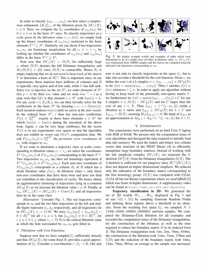
Fig. 3: We display example worlds and examples of paths which weredetermined to lie in a single class (in blue) at filtration value r2. DCr2 (X)was constructed from 100000 samples and the classes are computed using theindicated red trajectories corresponding to α0.

now is not only to classify trajectories in the space Cf , but totake into account a threshold for the cost function. Given c, wedefine the cost c of a k-simplex σ = {v0, . . . , vk} ∈ DCR(X)to be c(σ) = max(c(v0), . . . , c(vk)). Then c satisfies c(τ) 6c(σ) whenever τ ⊆ σ. In order to apply our algorithm withouthaving to keep track of the potentially non-sparse matrix V ,we furthermore let c(σ) = max(c(v0), . . . , c(vk))+C for anyk-simplex σ ∈ D(X) − DCR(X) and for C larger than thecost of any v ∈ X . Then LR,λ = c−1((−∞, λ]) yields afiltration as λ varies and LR,λ ⊆ DCR(X) for λ < C andLR,∞ = D(X), ensuring H1(LR,∞) = 0. We think of LR,λ asan approximation to MR,λ = XR ∩ c−1((−∞, λ]) for λ < C.

V. EXPERIMENTS

Our experiments were performed on an Intel Core i7 laptopwith 8GB of RAM. We present only the computation times ofcore algorithms and disregard the time required to initially loaddata into memory. We used the matrix and binary tree columnvector data structure of the PHAT library [4] to efficientlymanipulate large boundary matrices. Instead of working withthe full simplicial complex DCr(X), we extracted the 2-skeleton DC2

r (X) from the Delaunay triangulation D(X). The2-skeleton is sufficient for our purposes since Hi,j

1 (DCr(X))does not depend on higher dimensional simplices. We reducedonly the submatrix of the boundary matrix corresponding tothe first homology group. D(X) was computed with CGAL[1] for all but our Baxter experiments where we used QHull [2]which was faster in higher dimensions. A supplementary videocan be found at http://www.csc.kth.se/~fpokorny.

Trajectory classification in 2D: We generated theset of 2D worlds W1, . . . ,W10 displayed in Fig 3 andof size 512 × 512 by sampling Gaussian Random Fieldsand defining those regions above a threshold to be obsta-cles. From the resulting free space Cf , we sampled N ∈{1000, 10000, 100000, 1000000} uniform samples. We com-puted the Delaunay-Cech filtration for all examples andrecorded the computation times of the Delaunay triangulation,for the construction of the filtration, as well as the timerequired to reduce the boundary matrix D to its reduced formR. The Delaunay triangulation took 1ms, 2ms, 76ms, 810ms,the construction of the filtration took 11ms, 31ms, 278ms and3.27s and the reduction of the boundary matrix took 14ms,13ms, 76ms, 981ms on average as the sample size increased.

Fig. 4: We display the example world W1 with DCr2 (X) for 1000, 10000and 100000 sample points per row. In each column, we plot paths α1, . . . , αs

(in blue) which belong to a fixed trajectory class at filtration value r2. Thefixed reference path α0 is plotted in red. As expected, we can clearly seethat two paths in different classes also lie in different homotopy classes. Inour experiments, paths within a class are furthermore homotopy equivalentin DCr2 (X), but the quality of the approximation DCr2 (X) ' Cf is onlysufficient for 10000 or more sample points as can be seen in the right figurein the first row. There, some 2-simplices (triangles) cover the thin obstacleregion to the right.We investigated the filtration DCr(X) at various thresholds.At a filtration value of r1 = 25

√1000/N , we found that Cf

was conservatively covered, while at r2 = 35√

1000/N , thespace was well covered with a minimum number of holes incollision free areas. In order to investigate interesting pathclasses, we generated a set of 1000 paths per world andsample setting as follows: In 10 trials, we selected two samplepoints v1, v2 at random and, for each such setting, we selectedanother 100 random waypoints w1, . . . , w100 from the sampledpoint-cloud. We determined shortest edge-path from v1 to wiand then to v2 utilizing Dijkstra’s algorithm on the 1-skeletongraph of DCr1(X). The computation times for the persistentcycle coordinates for these paths were 1.8ms, 10ms, 115msand 1.75s for a batch of 100 query paths and for the respectivesample sizes on average. These encouraging timings suggestthat our framework could be used as a classification ‘blackbox’ e.g. for continuous trajectory optimization engines.

Trajectory classification in 4D: We consider the planarrobot arm displayed in the top left of Fig. 5 attached to thecentral black disk and with 4 joints θ1, . . . , θ4. We constrainθ1 ∈ [−π2 ,

π2 ], θ2, θ3, θ4 ∈ [−0.9π, 0.9π] and furthermore

disallow self-collisions and collisions with the environment(the black rectangle and the floor), yielding Cf ⊂ R4. Therobot now has the task of moving from the start configurationdisplayed in blue to the red goal joint configuration as shownin the top left figure. We sampled 100000 poses uniformlyin Cf using OpenRave [13] and applied our framework.DC2∞(X) had about 6.2 million triangles and 1.8 million

0 0.50

0.3010.382

0.5

Fig. 5: The top left figure shows the robot arm in start configuration (blue) onthe right and in goal configuration (red) on the left. The right figure displaysthe first persistence diagram for our reconstruction with one red point farabove the diagonal. A projection of the samples onto θ1, θ2 is shown in themiddle and an illustration of the difference between the two trajectory classesfor r ∈ [0.301, 0.382] is shown in the bottom left figure. In the first trajectoryclass (in red), the arm is extended to the left when passing under the narrowpassage while in the second class (in blue), the arm is extended to the right.

Fig. 6: We display a cost function and classes of trajectories (in blue)depending on a cost threshold and a path α0 (in red). For the higher thresholdin the rightmost plot, the two classes in the two leftmost figures merge.

edges. The right part of Fig. 5 displays the resulting firstpersistence diagram which clearly shows that a single homo-logical feature has large persistence in Cf . The projection ofthe joint configurations onto the first two angles, as shown inthe middle figure, confirms the existence of a single hole. Wecomputed 1000 edge-paths in DC0.25 between the start andend-configuration using 1000 random waypoints as before. Forfiltration values r ∈ [0.301, 0.382] only two trajectory classesexisted. The reduction of the boundary matrix took 0.46s,while the persistent cycle coordinates for all 1000 paths werecalculated in 0.55s. The Delaunay triangulation in R4 took251s, partially due to the increased dimension. Note howeverthat these results are not directly comparable to the 2D casesince methods for 2D Delaunay triangulations in CGAL [1]are especially optimized. We inspected the trajectories in eachhomology class and found that they were classified accordingto whether the second link was positioned to the left or to theright of the base link of the arm when θ1 = 0 as the armpassed the narrow passage (see the bottom left part of Fig. 5).Our framework hence allows the robot to discover the fact thattwo fundamentally different solution trajectory classes exist.

Filtrations with cost functions: We consider the freeconfiguration space Cf ⊂ R2 of size 250 by 500 with twoobstacles (in white) displayed in Fig. 6. We would now liketo distinguish not only between homotopy classes dependingon the obstacles in the configuration space, but also discernhow trajectories behave with respect to the two peaks of thecost function. The simplicial complex L10,λ(X) is displayedfor 10000 samples X and height values are determined by thecost function. At cost threshold λ = 90, the top of one of thehills defined by the cost-function is removed from the complexin the rightmost figure (indicated in blue), while at λ = 70 bothhills are truncated in the remaining figures. We sampled 100random paths in this configuration space by fixing the initial

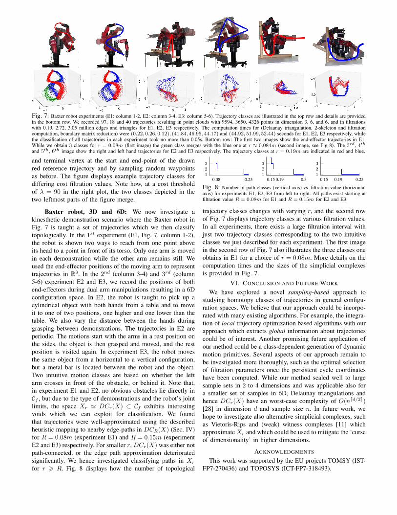
Fig. 7: Baxter robot experiments (E1: column 1-2, E2: column 3-4, E3: column 5-6). Trajectory classes are illustrated in the top row and details are providedin the bottom row. We recorded 97, 18 and 40 trajectories resulting in point clouds with 9594, 3650, 4326 points in dimension 3, 6, and 6, and in filtrationswith 0.19, 2.72, 3.05 million edges and triangles for E1, E2, E3 respectively. The computation times for (Delaunay triangulation, 2-skeleton and filtrationcomputation, boundary matrix reduction) were (0.22, 0.26, 0.12), (41.84, 46.95, 44.17) and (44.92, 51.99, 52.44) seconds for E1, E2, E3 respectively, whilethe classification of all trajectories in each experiment took no more than 0.05s. Bottom row: The first two images show the end-effector trajectories in E1.While we obtain 3 classes for r = 0.08m (first image) the green class merges with the blue one at r ≈ 0.084m (second image, see Fig 8). The 3rd, 4thand 5th, 6th image show the right and left hand trajectories for E2 and E3 respectively. The trajectory classes at r = 0.19m are indicated in red and blue.

and terminal vertex at the start and end-point of the drawnred reference trajectory and by sampling random waypointsas before. The figure displays example trajectory classes fordiffering cost filtration values. Note how, at a cost thresholdof λ = 90 in the right plot, the two classes depicted in thetwo leftmost parts of the figure merge.

Baxter robot, 3D and 6D: We now investigate akinesthetic demonstration scenario where the Baxter robot inFig. 7 is taught a set of trajectories which we then classifytopologically. In the 1st experiment (E1, Fig. 7, column 1-2),the robot is shown two ways to reach from one point aboveits head to a point in front of its torso. Only one arm is movedin each demonstration while the other arm remains still. Weused the end-effector positions of the moving arm to representtrajectories in R3. In the 2nd (column 3-4) and 3rd (column5-6) experiment E2 and E3, we record the positions of bothend-effectors during dual arm manipulations resulting in a 6Dconfiguration space. In E2, the robot is taught to pick up acylindrical object with both hands from a table and to moveit to one of two positions, one higher and one lower than thetable. We also vary the distance between the hands duringgrasping between demonstrations. The trajectories in E2 areperiodic. The motions start with the arms in a rest position onthe sides, the object is then grasped and moved, and the restposition is visited again. In experiment E3, the robot movesthe same object from a horizontal to a vertical configuration,but a metal bar is located between the robot and the object.Two intuitive motion classes are based on whether the leftarm crosses in front of the obstacle, or behind it. Note that,in experiment E1 and E2, no obvious obstacles lie directly inCf , but due to the type of demonstrations and the robot’s jointlimits, the space Xr ' DCr(X) ⊂ Cf exhibits interestingvoids which we can exploit for classification. We foundthat trajectories were well-approximated using the describedheuristic mapping to nearby edge-paths in DCR(X) (Sec. IV)for R = 0.08m (experiment E1) and R = 0.15m (experimentE2 and E3) respectively. For smaller r, DCr(X) was either notpath-connected, or the edge path approximation deterioratedsignificantly. We hence investigated classifying paths in Xr

for r > R. Fig. 8 displays how the number of topological

0.08 0.25123

0.15 0.19 0.3123

0.15 0.19 0.25123

Fig. 8: Number of path classes (vertical axis) vs. filtration value (horizontalaxis) for experiments E1, E2, E3 from left to right. All paths exist starting atfiltration value R = 0.08m for E1 and R = 0.15m for E2 and E3.

trajectory classes changes with varying r, and the second rowof Fig. 7 displays trajectory classes at various filtration values.In all experiments, there exists a large filtration interval withjust two trajectory classes corresponding to the two intuitiveclasses we just described for each experiment. The first imagein the second row of Fig. 7 also illustrates the three classes oneobtains in E1 for a choice of r = 0.08m. More details on thecomputation times and the sizes of the simplicial complexesis provided in Fig. 7.

VI. CONCLUSION AND FUTURE WORK

We have explored a novel sampling-based approach tostudying homotopy classes of trajectories in general configu-ration spaces. We believe that our approach could be incorpo-rated with many existing algorithms. For example, the integra-tion of local trajectory optimization based algorithms with ourapproach which extracts global information about trajectoriescould be of interest. Another promising future application ofour method could be a class-dependent generation of dynamicmotion primitives. Several aspects of our approach remain tobe investigated more thoroughly, such as the optimal selectionof filtration parameters once the persistent cycle coordinateshave been computed. While our method scaled well to largesample sets in 2 to 4 dimensions and was applicable also fora smaller set of samples in 6D, Delaunay triangulations andhence DCr(X) have an worst-case complexity of O(ndd/2e)[28] in dimension d and sample size n. In future work, wehope to investigate also alternative simplicial complexes, suchas Vietoris-Rips and (weak) witness complexes [11] whichapproximate Xr and which could be used to mitigate the ‘curseof dimensionality’ in higher dimensions.

ACKNOWLEDGMENTS

This work was supported by the EU projects TOMSY (IST-FP7-270436) and TOPOSYS (ICT-FP7-318493).

REFERENCES

[1] CGAL, Computational Geometry Algorithms Library.http://www.cgal.org.

[2] C. B. Barber, D. P. Dobkin, and H. Huhdanpaa. Thequickhull algorithm for convex hulls. ACM Trans. Math.Software, 22(4), 1996.

[3] U. Bauer and H. Edelsbrunner. The morse theory of Cechand Delaunay filtrations. In Proc. of the Thirtieth AnnualSymp. on Comp. Geometry, SOCG’14, pages 484:484–484:490, New York, NY, USA, 2014. ACM.

[4] U. Bauer, M. Kerber, and J. Reininghaus.PHAT (Persistent Homology Algorithm Toolbox).http://code.google.com/p/phat/.

[5] S. Bhattacharya, V. Kumar, and M. Likhachev. Search-based path planning with homotopy class constraints.In Proc. of The Twenty-Fourth AAAI Conf. on ArtificialIntelligence, Atlanta, Georgia, 11-15 July 2010.

[6] S. Bhattacharya, M. Likhachev, and V. Kumar. Identifi-cation and representation of homotopy classes of trajec-tories for search-based path planning in 3D. In Proc. ofRobotics: Science and Systems, 27-30 June 2011.

[7] S. Bhattacharya, D. Lipsky, R. Ghrist, and V. Kumar.Invariants for homology classes with application to opti-mal search and planning problem in robotics. Electronicpre-print, Aug 2012. arXiv:1208.0573.

[8] A. Billard, S. Calinon, R. Dillmann, and S. Schaal. Robotprogramming by demonstration. In Springer handbookof robotics, pages 1371–1394. Springer, 2008.

[9] O. Brock and O. Khatib. Real-time re-planning in high-dimensional configuration spaces using sets of homotopicpaths. In Proc. of the IEEE Int. Conf. on Robotics andAutomation (ICRA’00), 2000., volume 1, pages 550–555.IEEE, 2000.

[10] J. Canny. The complexity of robot motion planning. MITpress, 1988.

[11] G. Carlsson. Topology and data. Bull. Amer. Math. Soc.(N.S.), 46(2):255–308, 2009.

[12] C. Chen and M. Kerber. Persistent homology computa-tion with a twist. In Proc. of the 27th European Workshopon Computational Geometry, 2011.

[13] R. Diankov and J. Kuffner. OpenRAVE: A PlanningArchitecture for Autonomous Robotics. Technical ReportCMU-RI-TR-08-34, Robotics Institute, Pittsburgh, PA,July 2008.

[14] H. Edelsbrunner. The union of balls and its dual shape.Discrete and Comp. Geometry, 13(1):415–440, 1995.

[15] H. Edelsbrunner and J. Harer. Persistent homology-asurvey. Contemporary mathematics, 453:257–282, 2008.

[16] H. Edelsbrunner and J. L. Harer. Computational topol-ogy: an introduction. AMS Bookstore, 2010.

[17] L. Jaillet and T. Simeon. Path deformation roadmaps:Compact graphs with useful cycles for motion planning.Int. Journal of Robotics Research, 27(11-12):1175–1188,2008.

[18] L. Jaillet and T. Simeon. Path deformation roadmaps. InS. Akella, N. M. Amato, W. H. Huang, and B. Mishra,editors, Algorithmic Foundation of Robotics VII, vol-ume 47 of Springer Tracts in Advanced Robotics, pages19–34. Springer, 2008.

[19] S. Karaman and E. Frazzoli. Sampling-based algorithmsfor optimal motion planning. Int. Journal of RoboticsResearch, 30(7):846–894, 2011.

[20] L. E. Kavraki, P. Svestka, J.-C. Latombe, and M. H.Overmars. Probabilistic roadmaps for path planning inhigh-dimensional configuration spaces. IEEE Trans. onRobotics and Automation, 12(4):566–580, 1996.

[21] S. Kim, K. Sreenath, S. Bhattacharya, and V. Kumar.Optimal trajectory generation under homology class con-straints. In 51st IEEE Conf. on Decision and Control,10-13 Dec 2012.

[22] R. A. Knepper, S. S. Srinivasa, and M. T. Mason. Towarda deeper understanding of motion alternatives via anequivalence relation on local paths. Int. Journal ofRobotics Research, 31(2):167–186, 2012.

[23] J.-C. Latombe. Robot Motion Planning. Springer, 1991.[24] S. M. LaValle. Planning algorithms. Cambridge Univer-

sity Press, 2006.[25] S. M. LaValle and J. J. Kuffner. Rapidly-Exploring

Random Trees: Progress and Prospects. In B. R. Donald,K. M. Lynch, and D. Rus, editors, Algorithmic andComputational Robotics: New Directions, pages 293–308, Wellesley, MA, 2001. A K Peters.

[26] S. R. Lindemann and S. M. LaValle. Current issues insampling-based motion planning. In Robotics Research,pages 36–54. Springer, 2005.

[27] E. Masehian and D. Sedighizadeh. Classic and heuristicapproaches in robot motion planning - a chronologicalreview. World Academy of Science, Engineering andTechnology, 23:101–106, 2007.

[28] P. McMullen. The maximum numbers of faces of aconvex polytope. Mathematika, 17(02):179–184, 1970.

[29] B. Morris and M. Trivedi. Learning trajectory patterns byclustering: Experimental studies and comparative evalu-ation. In IEEE Int. Conf. on Comp. Vision and PatternRecognition (CVPR’09), pages 312–319. IEEE, 2009.

[30] P. Niyogi, S. Smale, and S. Weinberger. Finding thehomology of submanifolds with high confidence fromrandom samples. Discrete and Comp. Geometry, 39(1-3):419–441, 2008.

[31] J. T. Schwartz and M. Sharir. On the piano moversproblem. II. General techniques for computing topolog-ical properties of real algebraic manifolds. Advances inApplied Mathematics, 4(3):298–351, 1983.

[32] L. Zhang, Y. J. Kim, and D. Manocha. A hybrid approachfor complete motion planning. In Proc. of the IEEE/RSJInt. Conf. on Intelligent Robots and Systems, (IROS’07),pages 7–14. IEEE, 2007.

[33] Y. Zheng and X. Zhou. Computing with spatial trajec-tories. Springer, 2011.