Econometrica, Vol. 86, No. 3 (May, 2018), 775–804

Econometrica, Vol. 86, No. 3 (May, 2018), 775–804

LONG-RUN COVARIABILITY

ULRICH K. MÜLLERDepartment of Economics, Princeton University

MARK W. WATSONDepartment of Economics, Princeton University

We develop inference methods about long-run comovement of two time series. Theparameters of interest are defined in terms of population second moments of low-frequency transformations (“low-pass” filtered versions) of the data. We numericallydetermine confidence sets that control coverage over a wide range of potential bivari-ate persistence patterns, which include arbitrary linear combinations of I(0), I(1), nearunit roots, and fractionally integrated processes. In an application to U.S. economicdata, we quantify the long-run covariability of a variety of series, such as those givingrise to balanced growth, nominal exchange rates and relative nominal prices, the un-employment rate and inflation, money growth and inflation, earnings and stock prices,etc.

KEYWORDS: Bandpass regression, fractional integration, great ratios.

1. INTRODUCTION

ECONOMIC THEORIES OFTEN HAVE stark predictions about the covariability of vari-ables over long-horizons: consumption and income move proportionally (permanent in-come/life cycle model of consumption) as do nominal exchange rates and relative nominalprices (long-run PPP), the unemployment rate is unaffected by the rate of price inflation(vertical long-run Phillips curve), and so forth. But there is a limited set of statistical toolsto investigate the validity of these long-run propositions. This paper expands this set oftools.

Two fundamental problems plague statistical inference about long-run phenomena.The first is the paucity of sample information: there are few “long-run” observations inthe samples typically used in empirical analyses of long-run relations. The second is thatinference critically depends on the data’s long-run persistence. Random walks yield statis-tics with different probability distributions than i.i.d. data, for example, and observationsfrom persistent autoregressions or fractionally integrated processes yield statistics withtheir own unique probability distributions. Taken together, these two problems conspireto make long-run inference particularly difficult: proper inference depends critically onthe exact form of long-run persistence, but there is limited sample information availableto empirically determine this form.

This paper develops methods designed to provide reliable inference about long-run co-variability for a wide range of persistence patterns. The methods rely on a relatively smallnumber of low-frequency averages of the data to measure the data’s long-run variabil-ity and covariability. Our focus is on parameters that characterize the population secondmoments of these low-frequency averages.

Ulrich K. Müller: [email protected] W. Watson: [email protected] work was presented as the Fisher–Schultz lecture at the 2016 European meetings of the Economet-

ric Society. We thank David Papell, Ken West, three referees, and participants at several seminars for theircomments. Support was provided by the National Science Foundation through Grant SES-1627660.

© 2018 The Econometric Society https://doi.org/10.3982/ECTA15047

http://www.econometricsociety.org/

mailto:[email protected]

mailto:[email protected]

http://www.econometricsociety.org/

https://doi.org/10.3982/ECTA15047

776 U. K. MÜLLER AND M. W. WATSON

Our main contribution is to provide empirical researchers with a relatively easy-to-usemethod for constructing confidence intervals for long-run correlation coefficients, linearregression coefficients, and standard deviations of regression errors. These confidenceintervals are valid for I(0), I(1), near unit roots, fractionally integrated models, and linearcombinations of variables with these forms of persistence. Using a set of pre-computed“approximate least favorable distributions,” the confidence intervals readily follow fromthe formulae discussed in Section 4.1

The outline of the paper is as follows. The next section introduces two empirical ex-amples, the long-run relationship between consumption and GDP and between short-and long-term nominal interest rates, and defines the notion of long-run variability andcovariability used throughout the paper. Our definition involves the population secondmoments of long-run projections, where these projections are similar to low-pass filteredversions of the data (e.g., Baxter and King (1999) and Hodrick and Prescott (1997)). Inthe long-run projections we employ, long-run covariability is equivalently captured bythe covariability of a small number q of trigonometrically weighted averages of the data.The population second moments of the projections therefore correspond to an averageof the spectrum (or pseudo-spectrum when the spectrum does not exist) over a narrowlow-frequency band. Thus, this paper’s long-run covariance parameters are those fromlow-frequency band spectrum regression (as in Engle (1974)), extended to allow for pro-cesses with more than I(0) persistence. A key distinction between this paper and previoussemiparametric approaches to the joint low-frequency behavior of persistent time series(see, for instance, Phillips (1991), Marinucci and Robinson (2001), Chen and Hurvich(2003), Robinson and Hualde (2003), Robinson (2008), or Shimotsu (2012)) is that in ourasymptotic analysis, we keep q fixed as a function of the sample size. This ensures that thesmall-sample paucity of low-frequency information is reflected in our asymptotic approxi-mations, as in Müller and Watson (2008), which yields more reliable inference in samplestypically used in empirical macroeconomics.

Section 3 derives the large-sample normality of the q pairs of trigonometricallyweighted averages and introduces a flexible parameterization of the joint long-run per-sistence properties of the underlying stochastic process. The large-sample framework de-veloped in Section 3 reduces the problem of inference about long-run covariability pa-rameters into the problem of inference about the covariance matrix of a 2q-dimensionalmultivariate normal random vector. Section 4 reviews relevant methods for solving thisparametric small-sample problem. Section 5 uses the resulting inference methods andpost-WWII data from the United States to empirically study several familiar long-runrelations involving balanced growth (GDP, consumption, investment, labor income, andproductivity), the term structure of interest rates, the Fisher correlation (inflation and in-terest rates), the Phillips correlation (inflation and unemployment), PPP (exchange ratesand price ratios), money growth and inflation, consumption growth and real returns, andthe long-run relationship between stock prices, dividends, and earnings.

2. LONG-RUN PROJECTIONS AND COVARIABILITY

2.1. Two Empirical Examples of Long-Run Covariability

We begin by examining the long-run covariability of GDP and consumption and ofshort- and long-term nominal interest rates. These data motivate and illustrate the meth-ods developed in this paper.

1The replication file contains a matlab function for computing these confidence intervals and is available atwww.princeton.edu/~mwatson.

http://www.princeton.edu/~mwatson

LONG-RUN COVARIABILITY 777

Consumption and income: One of the most celebrated and studied long-run relation-ships in economics concerns income and consumption. The long-run stability of the con-sumption/income ratio is one of economics’ “Great Ratios” (Klein and Kosobud (1961))and even a casual glance at the U.S. data suggests the two variables move together closelyin the long run. Consider, for example, the evolution of U.S. real per-capita GDP and con-sumption over the post-WWII period. In the 17 years from 1948 through 1964, GDP in-creased by 62% and consumption increased by 52%. Over the next 17 years (1965–1981),both GDP and consumption grew more slowly, by only 30%. Growth rebounded during1982 to 1998, when GDP grew by 43% and consumption increased 55%, but slowed againover 1999–2015 when GDP grew by only 17% and consumption increased by only 23%.Over these 17-year periods, there was substantial variability in the average annual rateof growth of GDP (2.9%, 1.4%, 2.1%, and 0.9% per year, respectively over the subsam-ples), and these changes were roughly matched by consumption (annual average growthrates of 2.5%, 1.5%, 2.6%, and 1.2%). Thus, over periods of 17 years, GDP and consump-tion exhibited substantial long-run variability and covariability in the post-WWII sampleperiod.2

With this in mind, the first two panels of Figure 1 plot the average growth rates of GDPand consumption over six non-overlapping subsamples in 1948–2015. Figure 1(a) plotsthe average growth rates against time, and Figure 1(b) is a scatterplot of the six averagegrowth rates for consumption against the corresponding values for GDP. Each of the sixsubsamples contains roughly 11 years, spans of history longer than the typical businesscycle, and in this sense capture “long-run” variability in GDP and consumption. AverageGDP and consumption growth over these subsamples exhibited substantial variability and(from the scatterplot) roughly one-for-one covariability.

Figure 1(c) sharpens the analysis by plotting “low-pass” transformations of the seriesdesigned to isolate variation in the series with periods longer than 11 years, computedas projections onto low-frequency periodic functions. These low-frequency projectionsproduce series that are essentially the same as low-pass moving averages,3 but are easierto analyze. These low-frequency projections are computed as follows. Let xt , t = 1� � � � � Tdenote a time series (e.g., growth rates of GDP or consumption). We use cosine functionsfor the periodic functions; let Ψj(s) = √

2 cos(jsπ) denote the function with period 2/j(where the factor

√2 simplifies a calculation below), Ψ(s) = [Ψ1(s)�Ψ2(s)� � � � �Ψq(s)]′

denote a vector of these functions with periods 2 through 2/q, and ΨT denote the T × qmatrix with tth row given by Ψ((t − 1/2)/T)′, so the jth column of ΨT has period 2T/j.The GDP and consumption data in Figure 1 span T = 272 quarters, so setting q = 12captures periodicities longer than 272/6 ≈ 45 quarters, or 11.3 years. The projection of xt

onto Ψ((t − 1/2)/T) for t = 1� � � � �T yields the fitted values

xt = X ′TΨ

((t − 1/2)/T

)� (1)

where XT are the projection (linear regression) coefficients, XT = (Ψ ′TΨT )

−1Ψ ′Tx1:T , and

x1:T is the T × 1 vector with tth element given by xt . The fitted values from these pro-jections, say (xt� yt), are plotted in Figure 1(c) and evolve much like the averages in

2Consumption is personal consumption expenditures (including durables) from the NIPA; Section 5 showsresults for non-durables, services, and durables separately. Both GDP and consumption are deflated by thePCE deflator, so that output is measured in terms of consumption goods, and expressed in per-capita termsusing the civilian non-institutionalized population over the age of 16. The Supplemental Material (Müller andWatson (2018)) contains data sources and descriptions for all data used in this paper.

3The Supplemental Material provides a comparison.


(a) Average growth rates over subsamples (b) Average growth rates over subsamples

(c) Long-run projections (d) Long-run projections and projectioncoefficients

FIGURE 1.—Long-run average growth rates of consumption and GDP. Notes: Panel (a) shows sample aver-ages of the variables over the period shown. Panel (b) is a scatterplot of the variables in (a). Panel (c) plots theprojections of the data onto the low-frequency cosine terms discussed in the text, where sample means havebeen added to projections so they are consistent with the averages plotted in Figure 1(a). The small dots inpanel (d) are a scatterplot of the variables in (c) (after scaling) and the large circles are a scatterplot of theprojection coefficients (XjT �YjT ) from (c).

Figure 1(a), but better capture the smooth transition from high-growth to low-growthperiods.

The matrix ΨT has two properties that simplify calculations and interpretation of thelong-run projections. First, Ψ ′

T lT = 0, where lT is a vector of ones, so that xt also cor-responds to the projection of xt − x1:T onto Ψ((t − 1/2)/T), where x1:T is the samplemean. More generally, XT and xt are invariant to location shifts in the xt-process, so withxt = μ + ut , the properties of XT and xt do not depend on the typically unknown valueof μ.4 Second, T−1Ψ ′

TΨT = Iq, so XT corresponds to simple cosine-weighted averages ofthe data (i.e., are the “cosine transforms” of {xt})

XT = T−1Ψ ′Tx1:T � (2)

The orthogonality of the cosine regressors ΨT leads to a tight connection between thevariability and covariability in the long-run projections (xt� yt) plotted in Figure 1(c) and

4If the xt -process contains a linear trend, say xt = μ0 +μ2t +ut , then alternative periodic functions that areorthogonal to a time trend can be used so that XT and xt do not depend on (μ0�μ1). See Müller and Watson(2008) for one set of such functions.


the cosine transforms (XjT �YjT ):

T−1T∑t=1

(xt

yt

)(xt yt

) = T−1

(X ′

T

Y ′T

)Ψ ′

TΨT

(XT YT

) =(X ′

TXT X ′TYT

Y ′TXT Y ′

TYT

)� (3)

Thus, the sample covariability of the T time series projections (xt� yt) coincides with thesample covariability of the q projection coefficients/cosine transforms (XT �YT).5 This isshown in Figure 1(d), which shows a scatterplot of (scaled versions) of the projections(xt� yt), shown as small dots, and the projection coefficients (XjT �YjT ), shown as largecircles. While the scatterplots capture the same variability and covariability in long-runmovements in GDP and consumption growth, the projection coefficients eliminate muchof the serial correlation evident in the (xt� yt) scatterplot.

Short-term and long-term interest rates. The second empirical example involves short-and long-term nominal interest rates, as measured by the rate on 3-month U.S. Treasurybills, xt , and the rate on 10-year U.S. Treasury bonds, yt , from 1953 through 2015. Figure 2plots the levels of short- and long-term interest rates, (xt� yt), along with their long-runprojections, (xt� yt), and cosine transforms, (XT �YT ). This sample includes only 63 years,so periodicities longer than 11 years are extracted using long-run projections with q = 11.Figure 2(a) shows that these long-run projections capture the rise in interest rates fromthe beginning of the sample through the early 1980s and then their subsequent decline.The projections for long-term interest rates closely track the projections for short-termrates and, given the connection between the projections and cosine transforms, XjT andYjT are highly correlated (Figure 2(b)).

These two data sets differ markedly in their persistence: GDP and consumption growthrates are often modeled as low-order MA models, while nominal interest rates are highlyserially correlated. Yet, the variables in both data sets exhibit substantial long-run varia-tion and covariation which is readily evident in the long-run projections (xt� yt) or equiv-alently (from (3)) the projection coefficients (XT �YT ). This suggests that the covari-ance/variance properties of (XT �YT ) are a useful starting point for defining the long-runcovariability properties of stochastic processes exhibiting a wide range of persistent pat-terns.

(a) Interest rates and long-run projections (b) Long-run projection coefficients

FIGURE 2.—Long-run projections of short- and long-term interest rates. Notes: Panel (a) plots the projec-tions of the data onto the low-frequency cosine terms discussed in the text, where sample means have beenadded to projections so they are consistent with the levels of the data also shown in the figure. Panel (b) is ascatterplot of the projection coefficients (XjT �YjT ) from (a).

5Alternative low-frequency weights, such as Fourier transforms, have the same orthogonality properties andcould be used in place of the cosine transforms. While the general analysis accommodates these alternativeweights, our numerical analysis uses the cosine weights presented in the text.


2.2. A Measure of Long-Run Covariability Using Long-Run Projections

A straightforward definition of long-run covariability is based on the population ana-logue of the sample second moment matrices in (3). Let ΣT denote the covariance matrixof (X ′

T �Y′T )

′, partitioned as ΣXX�T , ΣXY�T , etc., and define

ΩT = T−1T∑t=1

E

[(xt

yt

)(xt yt

)](4)

=q∑

j=1

E

[(XjT

YjT

)(XjT

YjT

)′]=

(tr(ΣXX�T ) tr(ΣXY�T )

tr(ΣYX�T ) tr(ΣYY�T )

)�

where the equalities directly follow from (3).The 2 × 2 matrix ΩT is the average covariance matrix of the long-run projections (xt� yt)

in a sample of length T , and provides a summary of the variability and covariability of thelong-run projections over repeated samples. Equivalently, by the second equality, ΩT alsomeasures the covariability of the cosine transforms (XT �YT ). Corresponding long-runcorrelation and linear regression parameters follow from the usual formulae

ρT =Ωxy�T /√Ωxx�TΩyy�T �

βT =Ωxy�T /Ωxx�T �

σ2y|x�T =Ωyy�T − (Ωxy�T )

2/Ωxx�T �

(5)

where (Ωxy�T �Ωxx�T �Ωyy�T ) are the elements of ΩT . The linear regression coefficient βT

solves the population least-squares problem

βT = argminb

E

[T−1

T∑t=1

(yt − bxt)2

]� (6)

so that βT is the coefficient in the population best linear prediction of the long-run pro-jection yt by the long-run projection xt , σ2

y|x�T is the average variance of the predictionerror, and ρ2

T is the corresponding population R2. These parameters thus measure thepopulation linear dependence of the long-run variation of (xt� yt). Equivalently, by thesecond equality in (4), βT also solves

βT = argminb

E

[q∑

j=1

(YjT − bXjT )2

](7)

with a corresponding interpretation for σ2y|x�T and ρ2

T . Thus, these parameters equivalentlymeasure the (population) linear dependence in the scatterplots in Figures 1(d) and 2(b).

The covariance matrix, ΩT , or equivalently, (ρT �βT �σ2y|x�T ), are the long-run population

parameters that are the focus of our analysis. These parameters depend on the periodsused to define the “long run,” that is, the value of q used to construct the long-run projec-tions. In the empirical examples discussed above, we chose periods longer than 11 years,that is, periods longer than the U.S. business cycle. This led us to use q = 12 for GDPand consumption (with sample size T = 272 quarters) and q = 11 for interest rates (with


FIGURE 3.—Spectral weight for low frequencies with T = 272 quarters and q = 12. Notes: The figure plots|∑q

j=1

∑Tt=1 Ψj((t − 0�5)/T)e− i tφ|2 for frequencies 0 ≤ φ ≤ 2π/16. The horizontal axis is labeled with periods

measured in years (= 0�5π/φ).

sample size T = 252 quarters). If we had instead been interested in periods longer than20 years, we would have chosen q = 7 for GDP/consumption (2T/q ≈ 78 quarters) andq = 6 for interest rates (2T/q = 84 quarters). The important point is that q defines thelong-run periods of interest for the research question at hand.

2.3. Frequency Domain Interpretation of ΩT and (ρT �βT �σ2y|x�T )

The covariance matrix ΩT has a natural and familiar frequency domain interpretation.Since (XT �YT ) are weighted averages of the data zt = (xt� yt)

′, ΩT is a weighted averageof the variances and covariances of zt . If the time series are covariance stationary withspectral density matrix Fz(φ), these variances and covariances are weighted averages ofthe spectrum over different frequencies φ. In fact, a straightforward calculation shows(see the Supplemental Material) that ΩT = (2π)−1

∫ π

−πFz(φ)wT(φ)dφ, where wT(φ) =

|∑q

j=1

∑T

t=1 Ψj((t − 1/2)/T)e−itφ|2 and i = √−1.Figure 3 plots the weights wT(φ) for T = 272 quarters (the GDP-consumption sample

size) and q = 12, where the horizontal axis shows periods (in years) instead of frequency(annual period = 2π/(4φ)). The figure shows that ΩT is essentially a bandpass versionof the spectrum with periods between 2T (136 years) and T/6 (11.3 years) correspondingto cosine transforms with j = 1 through j = 12. Thus, ΩT and the associated values of(ρT �βT �σ

2y|x�T ) are bandpass regression parameters, as in Engle (1974), for a particular

low-frequency band. If, as in Engle’s analysis, the data are generated by an I(0) stochasticprocess, the spectrum is approximately flat over this band and inference follows relativelydirectly from classic results on spectral estimators (e.g., Brillinger (2001), Brockwell andDavis (1991)). However, if the process is not I(0) in the sense that the spectrum (orpseudo-spectrum) is not flat over this low-frequency band, I(0) procedures lead to faultyinference akin to Granger and Newbold’s (1974) spurious regressions. The goal of ouranalysis is to develop inference procedures that are robust to this I(0)-flat-spectrum as-sumption.


As discussed above, the upper frequency cutoff 2T/q, corresponding to 11 years inFigure 3, represents the highest low-frequency (shortest period) of interest for the re-searcher’s analysis and is problem-specific. The lower cutoff 2T , corresponding to 136years in Figure 3, is induced by the invariance to location shifts of the cosine transforms.Without knowledge of the population means, it is not possible to extract empirical infor-mation about arbitrarily low frequencies, and our estimand ΩT reflects this impossibility.What is more, the fact that the weight wT(φ) converges to zero as φ → 0 keeps our es-timand ΩT well-defined even for some (pseudo) spectra that diverge at frequency zero,such as for I(1) processes.

3. ASYMPTOTIC APPROXIMATIONS AND PARAMETERIZINGLONG-RUN PERSISTENCE AND COVARIABILITY

The long-run correlation and regression parameters from ΩT are functions of ΣT , thecovariance matrix of (XT �YT ). This section takes up two related issues. The first is theasymptotic normality of the cosine-weighted averages (XT �YT ). This serves as the basisfor the inference methods developed in Section 4 and provides large-sample approxi-mation for the matrices ΣT and ΩT . The second issue is a parameterization of long-runpersistence and comovement that determines the large-sample value of ΣT and ΩT .

3.1. Large-Sample Properties of Long-Run Sample Averages

Because (XT �YT ) are smooth averages of (xt� yt), a central limit theorem effect sug-gests that these averages are approximately Gaussian random variables under a range ofprimitive conditions about (xt� yt). The set of assumptions under which asymptotic nor-mality holds turns out to be reasonably broad, and encompasses many forms of potentialpersistence. Specifically, with zt = (xt� yt)

′, suppose that �zt has moving average repre-sentation �zt = CT(L)εt , where εt is a martingale difference sequence with non-singularcovariance matrix, �zt has a spectral density F�z�T , and εt and CT(L) satisfy other momentand decay restrictions given in Müller and Watson (2017, Theorem 1). The dependenceof CT and F�z�T on the sample size T accommodates many forms of persistence that re-quire double arrays as data generating process, such as autoregressive roots of the order1 − c/T , for fixed c.6

If the spectral density converges for all frequencies close to zero

T 2F�z�T (ω/T)→ S�z(ω) (8)

in a suitable sense, then

√T

(XT

YT

)⇒

(X

Y

)∼N (0�Σ)� (9)

and the finite-sample second moment matrix correspondingly converges to its large-sample counterpart (Müller and Watson (2017, Lemma 2)):

T Var(XT

YT

)= TΣT → Σ� (10)

6We omit the corresponding dependence of zt = (xt� yt)′ on T to ease notation.


The scaling necessary to achieve (8) is subsumed in CT(L). For instance, if xt is a randomwalk, and yt is i.i.d., then CT(L) = diag(1/T�1 −L) induces (8).

The limiting covariance matrix Σ in (9) and (10) is a function of the (pseudo) “local-to-zero spectrum” Sz(ω) = S�z(ω)/ω2 of zt and the cosine weights Ψj(s) that determine(XT �YT); specifically, from Müller and Watson (2017),

Σ=∫ ∞

−∞

(I2 ⊗

∫ 1

0eiλsΨ(s)ds

)′Sz(ω)

(I2 ⊗

∫ 1

0e−iλsΨ(s)ds

)dω�

These limiting results are consistent with the results for T = 272 shown in Figure 3 inthe previous section: (XT �YT) are low-frequency weighted averages of the data and theircovariance matrix depends on the (pseudo-) spectrum of (xt� yt) in a small band aroundfrequency zero.

We make three comments about these large-sample results. First, they hold when thefirst difference of zt has a spectral density; the level of zt is more persistent than its firstdifference and may have a (pseudo-) spectrum that diverges at frequency zero. In thiscase, Σ remains finite because the cosine averages sum to zero (Ψ ′

T lT = 0), so they donot extract zero-frequency variation in the data. If the level of zt has a spectral density,then this restriction on the weights is not required and, for example, the centered samplemean of zt also has a large-sample normal limit. Second, for zt ∼ I(d), the decay restric-tions on CT(L) allow values of d ∈ (−0�5�1�5), which allows a reasonably wide range ofpersistent processes, but rules out some models of practical interest. For example, thefirst difference of an I(0) process appended to a linear trend (i.e., the first differenceof a “trend-stationary” process) is I(−1) and is ruled out. And, of course, it does notaccommodate I(d) processes with d > 1�5. Third, because TΣT → Σ, also TΩT → Ωwhere Ω is defined as in the last expression of (4) with Σ in place of ΣT . Correspondingly,(ρT �βT �Tσ

2y|x�T )→ (ρ�β�σ2

y|x) with the limits defined by (5) with Ω in place of ΩT . Thus,a solution to the problem of inference about (ρ�β�σ2

y|x) given observations (X�Y) read-ily translates into a solution to large-sample valid inference about (ρT �βT �σ

2y|x�T ) given

(XT �YT), and, by invoking the arguments in Müller (2011), efficient inference in the for-mer problem amounts to large-sample efficient inference in the latter problem.

3.2. Parameterizing Long-Run Persistence and Covariability

The limiting average covariance matrix of the long-run projections, Ω, is a function ofthe covariance matrix of the cosine projections, Σ, which in turn is a function of the local-to-zero spectrum Sz of zt . In this section, we discuss parameterizations of Sz , and thus Σand Ω.

It is constructive to consider two leading examples. In the first, zt is I(0) with long-runcovariance matrix Λ. In this case, while the spectrum Fz�T (φ) potentially varies acrossfrequencies φ ∈ [−π�π], the local-to-zero spectrum is flat Sz(ω) ∝ Λ. Straightforwardcalculations then show that Σ = Λ ⊗ Iq and Ω = Λ, so the covariance matrix associatedwith the long-run projections corresponds to the usual long-run I(0) covariance matrix.In this model, the cosine transforms (XjT �YjT ) plotted in Figures 1 and 2 are, in largesamples and up to a deterministic scale, i.i.d. draws from a N (0�Λ) distribution. Infer-ence about Ω = Λ and (ρ�β�σ2

y|x) thus follows from well-known small-sample inferenceprocedures for Gaussian data (see Müller and Watson (2017)). In the second example,zt is I(1) with Λ the long-run covariance matrix for �zt . In this case, Sz(ω) ∝ ω−2Λ, and


TABLE I

LONG-RUN COVARIABILITY ESTIMATES AND CONFIDENCE INTERVALS USING THE I(0) AND I(1) MODELS:PERIODS LONGER THAN 11 YEARS

ρ β σy|x

a. GDP and consumptionI(0) Estimate 0.93 0.76 0.36

67% CI 0.87, 0.96 0.67, 0.85 0.30, 0.4690% CI 0.80, 0.97 0.60, 0.92 0.27, 0.55

I(1) Estimate 0.93 0.84 0.3567% CI 0.88, 0.96 0.74, 0.94 0.29, 0.4590% CI 0.82, 0.97 0.66, 1.01 0.26, 0.54

b. Short- and long-term interest ratesI(0) Estimate 0.98 0.96 0.60

67% CI 0.96, 0.98 0.90, 1.03 0.50, 0.7990% CI 0.93, 0.99 0.84, 1.08 0.44, 0.96

I(1) Estimate 0.97 0.93 0.3867% CI 0.93, 0.98 0.85, 1.01 0.32, 0.5090% CI 0.90, 0.98 0.78, 1.07 0.28, 0.61

Notes: Periods longer than 11 years correspond to q = 12 for panel (a) and q = 11 for panel (b). The rows labeled “Estimate” arethe maximum likelihood estimates using the large-sample distribution of the cosine transforms for the I(0) and I(1) models and therows labeled “CI” denote the associated confidence intervals.

a calculation shows that Σ = Λ ⊗ D, where D is a q× q diagonal matrix with jth di-agonal element Djj = (jπ)−2. In this model, the cosine transforms (XjT �YjT ) plotted inFigures 1 and 2 are, in large samples and up to a deterministic scale, independent butheteroscedastic draws from N (0� (jπ)−2Λ) distributions. Thus Ω ∝ Λ, so the covariancematrix for long-run projections for zt corresponds to the long-run covariance matrix forits first differences, �zt . By weighted least-squares logic, inference for I(1) processes fol-lows after reweighting the elements of (XjT �YjT ) by the square roots of the inverse of thediagonal elements of D and then using the same methods as in the I(0) model.

GDP and consumption and short-term and long-term interest rates: Table I presents esti-mates and confidence sets for (ρT �βT �σy|x�T ) using (XT �YT ) for GDP and consumption(panel (a)) and for short- and long-term interest rates (panel (b)), where the focus ison periods longer than 11 years, so that q = 12 for panel (a) and q = 11 for panel (b).Results are presented for I(0) and I(1) models; a more general model of persistenceis introduced below. The point estimates shown in the table are MLEs, and confidenceintervals for (βT �σ

2y|x�T ) are computed using standard finite-sample normal linear regres-

sion formulae (after appropriate weighting in I(1) model), and confidence sets for ρT areconstructed as in Anderson (1984, Section 4.2.2).

For GDP and consumption, there are only minor differences between the I(0) and I(1)estimates and confidence sets. The estimated long-run correlation is greater than 0.9, andthe lower range of the 90% confidence interval exceeds 0.8 in both the I(0) and I(1)models. Thus, despite the limited long-run information in the sample (captured here bythe 12 observations making up (XT �YT )), the evidence points to a large long-run correla-tion between GDP and consumption. The long-run regression of consumption onto GDPyields a regression coefficient that is estimated to be 0.76 in the I(0) model and 0.84 inthe I(1) model. This estimate is sufficiently accurate that β= 1 is not included in the 90%I(0) confidence set. The results for long-term and short-term nominal interest rates are


similarly informative: there is strong evidence that the series are highly correlated overthe long run.

The validity of these confidence sets rests on the quality of the I(0) and I(1) models forapproximating the spectral shape over the low-frequency band plotted in Figure 3. TheI(0) model assumes the spectrum is flat over this band, so the series behave like whitenoises for periods longer than 11 years, while the I(1) model assumes random-walk be-havior. Neither assumption is particularly compelling. Moreover, as we show in Table IVbelow, the I(0) assumption yields confidence intervals with coverage probability far be-low the nominal level when, in fact, the data were generated by the I(1) model, and viceversa, and both yield faulty inference when persistence is something other than I(0) orI(1). With this motivation, the next subsection proposes a more flexible parameterizationof persistence.

3.2.1. (A�B� c�d) Model

The shape of the local-to-zero spectrum determines the long-run persistence proper-ties of the data, and misspecification of this persistence leads to faulty inference aboutlong-run covariability. Simply put, reliable inference requires a parameterization of thespectrum that yields a good approximation to the persistence patterns of the variablesover the low-frequency band under study. Addressing this issue faces a familiar trade-off: the parameterization needs to be sufficiently flexible to yield reliable inference aboutlong-run covariability for a wide range of economically relevant stochastic processes andyet be sufficiently parsimonious to allow meaningful inference with limited sample in-formation. I(0) persistence generates a flat local-to-zero spectrum, and I(1) persistencegenerates a local-to-zero spectrum proportional to ω−2. Both of these models are parsi-monious, but tightly constrain the spectrum. This limits their usefulness as general modelsfor conducting inference about long-run covariability.

With this trade-off in mind, we use a parameterization that nests and generalizes arange of models previously used to model persistence in economic time series. The pa-rameterization is a bivariate extension of the univariate (b� c�d) model used in Müllerand Watson (2016) and yields a local-to-zero spectrum of the form

Sz(ω)∝A

((ω2 + c2

1

)−d1 0

0(ω2 + c2

2

)−d2

)A′ +BB′� (11)

where A and B are 2 × 2 matrices with A unrestricted and B lower triangular.7The primary motivation for this (A�B� c�d) model is as a parsimonious but flexible

functional form for the local-to-zero spectrum. It combines and generalizes several stan-dard spectral shapes. For example, with A = 0, it is the I(0) local-to-zero spectrum. WhenB = 0, c = 0, and d1 = d2 = 1, it yields the I(1) spectrum; B = 0, d1 = d2 = 1 yields a spec-trum for arbitrary linear combinations of two independent local-to-unity processes withmean reversion parameters equal to c1 and c2; B = 0 and c = 0 yields a bivariate frac-tional spectrum with parameters d1 and d2. Other choices of (A�B� c�d) yield spectrafrom models that combine persistent and non-persistent components (as in cointegratedor “local-level” models) but go beyond the usual I(0)/I(1) or fractional formulations.

7This is the spectrum of a bivariate Whittle–Matérn (cf. Lindgren (2013)) process with time series rep-resentation zt = Aτt + et , where τt = (τ1t � τ2t )

′ is a bivariate process with uncorrelated {τ1t} and {τ2t},(1 −φi�TL)

di τit = T−di/2εit , φi�T = 1 − ci/T , εt ∼ I(0) with long-run variance equal to I2, et ∼ I(0) with long-run variance equal to BB′, and zero long-run covariance with εt .


The nesting of the cointegrated model in the (A�B� c�d) model is particularly interest-ing because it, too, focuses on long-run relationship between the variables. Formally, ofcourse, cointegration concerns common patterns of persistence in the variables, not theirvariance and covariance: in its canonical form, xt and yt are cointegrated if both are I(1)and yet a linear combination of the variables is I(0). This implies that the variables sharea single I(1) trend in addition to I(0) components. When the innovations of the I(1) andI(0) components are of the same order of magnitude, then the spectrum is dominated bythe I(1) component over low frequencies. Thus, in the context of the (A�B� c�d) model,the canonical cointegration model corresponds to the restrictions B = 0 (because themarginal processes are dominated by the stochastic trends), c1 = c2 = 0 and d1 = d2 = 1(so the trend components are I(1)), and A has rank 1 (because there is a single commontrend). The singularity in A in turn induces singularities in Sz and Σ. The large-T limit ofthe usual formulation of cointegration thus implies that long-run projections computedwith a fixed value of q are perfectly correlated, and the scatterplot of projection coeffi-cients lies on a straight line with slope corresponding to the cointegrating coefficient. Ofcourse, this perfect correlation will not obtain with finite T , so practically useful approxi-mations would require a non-singular value of A and/or a non-zero value of B.

3.2.2. Beyond the (A�B� c�d) Model

While the (A�B� c�d) parameterization encompasses many standard models, it is use-ful to highlight some models that are not encompassed by (11). We discuss two here.

One restriction of the (A�B� c�d) model is the asymptotic independence of the persis-tent and I(0) components, as captured by A and B, respectively. One model where thisindependence is restrictive is in a cointegrated model with a local-to-zero cointegrationcoefficient and correlated I(0) and trend components. Consider, for instance, a modelwhere xt is the stochastic trend, and yt is a linear combination of an I(0) error correc-tion term and xt , with a coefficient on xt that is of order 1/T .8 Allowing xt to follow alocal-to-unity process, the model is

xt = (1 − c/T)xt−1 + ux�t�

yt = η

Txt + uy�t�

(12)

where ut = (ux�t� uy�t) is I(0) with long-run covariance Σu and elements σ2x , σ2

y , and λσxσy

in obvious notation. The corresponding local-to-zero spectral density is

Sz(ω) ∝(σx 0η σy

)((ω2 + c2

)−1λ(c + iω)−1

λ(c − iω)−1 1

)(σx η

0 σy

)� (13)

This “local cointegration” spectral density is outside the (A�B� c�d) model wheneverλ �= 0. The complex-valued local-to-zero spectral density indicates the presence of leadand lag relationships that span a non-trivial fraction of the sample size. Since the level ofxt depends in a non-negligible manner on values of ux�s with s t, xt is correlated withvalues of uy�s in the distant past when λ �= 0.

In this model, a calculation shows that the population regression of Y onto X has a re-gression coefficient β= η+λc, so it depends on the local cointegrating coefficient η, the

8Given the invariance restrictions we impose in Section 4.2.1 below, such a transformation of the cointegra-tion model is without loss of generality for inference about βT and σ2

y|x�T .


I(0) correlation coefficient λ, and the persistence parameter c. In contrast, previous anal-yses of the model (12) (see, for instance, Elliott (1998) or Jansson and Moreira (2006))focused on the cointegration parameter η. This difference emphasizes the distinct goalsof the analyses: The cointegration parameter η yields the linear combination of (x� y)with minimum persistence, while the regression parameter β yields the linear combina-tion with minimum variance. In general, there is no reason to expect that these are thesame, and this makes it is surprising that these two goals yield the same estimand (β= η)in the canonical cointegration model with c = 0, even for λ �= 0.

There are many other ways of modeling the joint long-run properties of zt . As alreadymentioned, since the (A�B� c�d) model has a real-valued local-to-zero spectrum, it rulesout long-span leads and lags between the series. One simple way to generate such lags isvia

xt =A11u1�t +A12u2�t−�δT ��

yt =A21u1�t +A22u2�t−�δT ��(14)

where ut ∼ I(0) as above. The parameter δ ∈ R measures the lead of u1�t relative tou2�t−�δT � as a fraction of the sample size. In this “I(0) long-lag” model, the local-to-zerospectral density satisfies

Sz(ω) ∝A

(σx λσxσy exp(iδω)

λσxσy exp(−iδω) σy

)A′ (15)

with [A] = Aij . When λ �= 0, the long lags relating x and y yield a complex local-to-zerocross spectrum which is outside the (A�B� c�d) class.

Our construction does not guarantee that confidence sets have their desired coverageprobabilities outside the (A�B� c�d) model; we present numerical results in Section 4.3below that investigate the magnitude of inference errors associated with models (13) and(15).

4. CONSTRUCTING CONFIDENCE INTERVALS FOR ρ, β, AND σy|x

4.1. An Overview

There are several approaches one might take to construct confidence intervals for theparameters ρ, β, and σy|x from the observations (X�Y). As a general matter, the goal isto compute confidence intervals that are as informative (“short”) as possible, subject tothe coverage constraint that they contain the true value of the parameter of interest with apre-specified probability. We construct confidence intervals by explicitly solving a versionof this problem.

Generically, let θ denote the vector of parameters characterizing the probability distri-bution of (X�Y), and let Θ denote the parameter space. (In our context, θ denotes the(A�B� c�d) parameters.) Let γ = g(θ) denote the parameter of interest. (γ = ρ, β, orσy|x for the problem we consider.) Let H(X�Y) denote a confidence interval for γ andlgth(H(X�Y)) denote the length of the interval. The objective is to choose H so it hassmall expected length, E[lgth(H(X�Y)], subject to coverage, P(γ ∈ H(X�Y)) ≥ 1 − α,where α is a pre-specified constant. Because the probability distribution of (X�Y) de-pends on θ, so will the expected length of H(X�Y ) and the coverage probability. Bydefinition, the coverage constraint must be satisfied for all values of θ ∈ Θ, but one hasfreedom in choosing the value of θ over which expected length is to be minimized. Thus,


let W denote a distribution that puts weight on different values of θ, so the problem be-comes

minH

∫Eθ

[lgth

(H(X�Y)

)]dW (θ) (16)

subject to

infθ∈Θ

Pθ

(γ ∈ H(X�Y)

) ≥ 1 − α� (17)

where the objective function (16) emphasizes that the expected volume depends on thevalue of θ, with different values of θ weighted by W , and the coverage constraint (17)emphasizes that the constraint must hold for all values of θ in the parameter space Θ.

As noted by Pratt (1961), the expected length of confidence set for γ can be expressedin terms of the power of hypothesis tests of H0 : γ = γ0 versus H1 : θ ∼ W . The solutionto (16)–(17) thus amounts to the determination of a family of most powerful hypothesistests, indexed by γ0. Elliott, Müller, and Watson (2015) suggested a numerical approach tocompute corresponding approximate “least favorable distributions” for θ. We implementa version of those methods here; details are provided in the Supplemental Material. A keyfeature of the solution is that, conditional on the weighting function W and the leastfavorable distribution, the confidence sets have the familiar Neyman–Pearson form witha version of the likelihood ratio determining the values of γ included in the confidenceinterval.

While the resulting confidence intervals have smallest weighted expected length (upto the bounds used in the numerical approximation of the least favorable distributions),they can have unreasonable properties for particular realizations of (X�Y). Indeed, forsome values of (X�Y), the confidence intervals might be empty, with the uncomfortableimplication that, conditional on observing these values of (X�Y), one is certain that theconfidence interval excludes the true value. To avoid this, we follow Müller and Norets(2016) and restrict the confidence sets to be supersets of 1−α equal-tailed Bayes crediblesets.

4.2. Some Specifics

4.2.1. Invariance and Equivariance

Correlations are invariant to the scale of the data. The linear regression of yt ontoxt is the same as the regression of yt + bxt onto xt after subtracting b from the latter’sregression coefficient. It is sensible to impose the same invariance/equivariance on theconfidence intervals. Thus, letting Hρ, Hβ, and Hσ denote confidence sets for ρ, β, andσy|x, we restrict these sets as follows:

ρ ∈ Hρ(X�Y) ⇔ ρ ∈ Hρ(bxX�byY) for bxby > 0� (18)

β ∈Hβ(X�Y)

⇔ byβ+ byx

bx

∈Hβ(bxX�byY + byxX) for bx�by �= 0 and all values of byx�(19)

σy|x ∈ Hσ(X�Y)

⇔ |by |σy|x ∈ Hσ(bxX�byY + byxX) for bx�by �= 0 and all values of byx�(20)


These invariance/equivariance restrictions lead to two modifications to the solution to(16)–(17). First, they require the use of maximal invariants in place of the original (X�Y).The density of the maximal invariants for each of these transformations is derived in theSupplemental Material. Second, because the objective function (16) is stated in termsof (X�Y), minimizing expected length by inverting tests based on the maximal invariantleads to a slightly different form of optimal test statistic. Müller and Norets (2016) devel-oped these modifications in a general setting, and the Supplemental Material derives theresulting form of confidence sets for our problem.

4.2.2. Parameter Space

We use the following parameter space for θ = (A�B� c�d): A and B are real, with Blower-triangular and (A�B) chosen so that Ω is non-singular, ci ≥ 0, and −0�4 ≤ di ≤ 1,for i = 1�2.9 Thus, the confidence intervals control coverage over a wide range of persis-tence patterns including processes less persistent than I(0), as persistent as I(1), local-to-unity autoregressions, and where different linear combinations of xt and yt may havemarkedly different persistence. Even though our theoretical development would allow forvalues of di up to 1�5, we consider values of di > 1 reasonably rare in empirical analysis ofeconomic time series. In order to obtain more informative inference, we therefore restrictthe parameter space to −0�4 ≤ di ≤ 1, for i = 1�2.

The confidence sets we construct require three distributions over θ: the weighting func-tion W for computing the average length in the objective (16), the Bayes prior associatedwith the Bayes credible sets that serve as subsets for the confidence sets (Müller andNorets (2016)), and the least favorable distribution for θ that enforces the coverage con-straint. The latter is endogenous to the program (16)–(17) and is approximated usingnumerical methods similar to those discussed in Elliott, Müller, and Watson (2015), withdetails provided in the Supplemental Material. In our baseline analysis, we use the samedistribution for W and the Bayes prior. Specifically, this distribution is based on the bi-variate I(d) model (so that c1 = c2 = 0, B = 0) with d1 and d2 independently distributedU(−0�4�1�0). Because of the invariance/equivariance restrictions, the scale of the matrixA is irrelevant and we set A =R(λ1)G(s)R(λ2), where R(λ) is a rotation matrix indexedby the angle λ, with λ1 and λ2 independently distributed U[0�π]. The relative eigenval-ues of A are determined by the diagonal matrix G(s), with G11/G22 = 15s with s inde-pendently distributed U[0�1]. We investigate the robustness of this choice in Section 4.3below.

4.2.3. Empirical Results for GDP, Consumption, and Interest Rates

Table II shows estimates for (ρT �βT �σy|x�T ) and confidence sets using the (A�B� c�d)model. The estimated value of (ρT �βT �σy|x�T ) is the median of the posterior using theI(d)-model prior, and the table also shows Bayes credible sets for this prior for compari-son with the frequentist confidence intervals. For GDP and consumption, the (A�B� c�d)results look much like the results obtained for the I(0) model shown in Table I. For mostentries, the Bayes credible sets are slightly larger than the I(0) sets, presumably reflectingthe possibility of persistence greater than I(0). The frequentist confidence intervals oftencoincide with Bayes intervals, but occasionally are somewhat wider. The results indicatethat GDP and consumption are highly correlated in the long run (the 90% confidenceset is 0�71 ≤ ρ ≤ 0�97) and the long-run regression coefficient of consumption onto GDP

9See the Appendix for additional details.


TABLE II

LONG-RUN COVARIABILITY ESTIMATES, CONFIDENCE INTERVALS AND CREDIBLE SETS USING THE(A�B�C�D) MODELS: PERIODS LONGER THAN 11 YEARS

ρ β σy|x

a. GDP and consumption(A�B� c�d) Estimate 0.91 0.77 0.41

67% CI 0.83, 0.96 0.66, 0.87 0.33, 0.5390% CI 0.71, 0.97 0.48, 0.96 0.29, 0.6667% Bayes CS 0.83, 0.96 0.66, 0.87 0.33, 0.5390% Bayes CS 0.71, 0.97 0.58, 0.96 0.29, 0.66

b. Short- and long-term interest rates(A�B� c�d) Estimate 0.96 0.95 0.63

67% CI 0.92, 0.98 0.87, 1.07 0.49, 0.9790% CI 0.89, 0.99 0.76, 1.16 0.42, 1.2767% Bayes CS 0.92, 0.98 0.87, 1.03 0.49, 0.8290% Bayes CS 0.89, 0.99 0.81, 1.09 0.42, 1.02

Notes: Periods longer than 11 years correspond to q = 12 for panel (a) and q = 11 for panel (b). The rows labeled “Estimate” arethe posterior median based on the I(d) model. “CI” denotes confidence interval, which is calculated as described in the text. “BayesCS” are Bayes equal-tailed credible sets based on the posterior from the I(d) model.

is large, but less than unity (the 90% confidence set is 0�48 ≤ β ≤ 0�95). The results forinterest rates indicate that long-run movements in short and long rates are highly corre-lated, and that these data are consistent with a unit long-run response of long rates toshort rates.

4.3. Asymptotic Power and Size

In this subsection, we investigate some aspects of power and size that govern the aver-age length and coverage of the confidence intervals. For power, we investigate the choiceof the weighting function W and the restriction of our confidence sets to be supersets of1 − α Bayes credible sets. For size, we investigate the non-coverage probability of confi-dence intervals constructed for misspecified models. To keep the discussion concise, wefocus exclusively on tests of H0 : ρ= 0 of level α= 10% using q = 12 in this subsection.

We first consider variations in weighting functions W and the cost of imposing theBayes superset restriction. We investigate three weighting functions: the baseline weight-ing function W = Wbase described above, the weighting function WI(0) that is equivalent toWbase except that d1 = d2 = 0, and WI(1) obtained by setting d1 = d2 = 1. For each W , wecompute the weighted average power maximizing test, both with and without the restric-tion that the implied confidence set is a superset of the 1 − α Bayes credible set underthe prior Wbase. This results in six tests. For each test, we then compute its weighted aver-age power, under each of the three weighting functions. In other words, we compute thepower of the six tests of H0 : ρ = 0 against the alternative that the data were generatedby θ randomly drawn from W , for each of the three W . Table III shows the results. Con-sider first tests that do not impose the Bayes superset restriction. By construction, the testthat is constructed to maximize weighted average power against a given W has the high-est weighted average power against that W among all level-α tests; these power-envelopevalues are shown in the diagonal entries in the table. The table indicates that the optimaltest for WI(0) has substantially less power under WI(1) than this envelope, and vice versa.The test constructed under Wbase, in contrast, is essentially on the envelope under WI(0),


TABLE III

ASYMPTOTIC WEIGHTED AVERAGE POWER OF 10% LEVEL EFFICIENT TEST OF H0: ρ= 0 IN (A�B� c�d)MODEL (q = 12)

WAP efficient test for

WI(0) WI(1) Wbase WI(0) WI(1) Wbase

WAP computed for without Bayes superset constraint with Bayes superset constraint

WI(0 0.69 0.34 0.69 0.64 0.34 0.64WI(1) 0.38 0.66 0.60 0.38 0.65 0.60Wbase 0.57 0.41 0.61 0.55 0.41 0.58

Notes: The entries are the asymptotic weighted average power over alternatives shown in rows using WAP efficient tests foralternatives given in columns.

and loses only about 6 percentage points under WI(1). Turning to the comparison withtests that impose the Bayes superset restriction, the table suggests that its cost in terms ofweighted average power is fairly small, especially under Wbase.

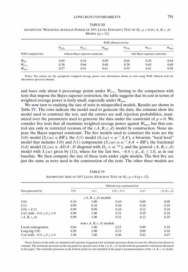
We now turn to studying the size of tests in misspecified models. Results are shown inTable IV. The rows indicate the model used to generate the data, the columns show themodel used to construct the test, and the entries are null rejection probabilities, maxi-mized over the parameters used to generate the data under the constraint of ρ = 0. Weconsider five tests that all maximize weighted average power against Wbase, but that con-trol size only in restricted versions of the (A�B� c�d) model by construction. None im-pose the Bayes superset constraint. The five models used to construct the tests are theI(0) model (Sz(ω) ∝ BB′), the I(1) model (Sz(ω) = ω−2AA′), a bivariate “local level”model that includes I(0) and I(1) components (Sz(ω) ∝ ω−2AA′ + BB′), the fractionalI(d) model (Sz(ω) ∝ ADA′, D diagonal with Djj = ω−2dj ), and the general (A�B� c�d)model with Sz(ω) given by (11), where for the last two, −0�4 ≤ d1� d2 ≤ 1�0, as in ourbaseline. We then compute the size of these tests under eight models. The first five arejust the same as were used in the construction of the tests. The other three models are

TABLE IV

ASYMPTOTIC SIZE OF 10% LEVEL EFFICIENT TEST OF H0: ρ = 0 (q = 12)

Efficient test constructed for

Data generated by I(0) I(1) I(0)+ I(1) I(d) (A�B� c�d)

(A�B� c�d) modelsI(0) 0.10 1.00 0.10 0.09 0.09I(1) 0.99 0.10 0.10 0.10 0.10I(0)+ I(1) 0.99 0.99 0.10 0.12 0.10I(d) with −0�4 ≤ d ≤ 1�0 0.99 1.00 0.31 0.10 0.10(A�B� c�d) 0.99 1.00 0.31 0.13 0.10

non-(A�B� c�d) modelsLocal cointegration 0.84 1.00 0.15 0.09 0.10Long-lag I(0) 0.30 1.00 0.13 0.09 0.10I(d) with −0�4 ≤ d ≤ 1�4 1.00 1.00 0.46 0.42 0.47

Notes: Entries in the table are maximal null rejection frequencies for stochastic processes shown in rows for efficient tests shown incolumns. The stochastic processes in the top panel are special cases of the (A�B� c�d) model with the parametric restrictions discussedin the paper. The stochastic processes in the bottom panel are not included in the paper’s parameterization of the (A�B� c�d) model.


the local cointegration model (13), the long-lag I(0) model (15), and the fractional modelwith −0�4 ≤ d1� d2 ≤ 1�4. The table therefore shows sizes computed from 40 experimentscomposed of five different tests and data generated from eight different stochastic pro-cesses.

The top panel of the table shows results for data generated by each of the five modelsused to construct the tests, so the diagonal entries of the table are equal to 0.10 by con-struction. The off-diagonal entries larger than 0.10 indicate size distortions. For example,the 10-percent level I(0) test mistakenly rejects for 99 percent of the draws when the dataare generated by other models. The I(1) test has similarly large size distortions when thedata are not generated by the I(1) model. These results mirror previous findings of thefragility of inference based on the assumption of exact I(0) or I(1) persistence patterns(e.g., den Haan and Levin (1997) for HAC inference in I(0) models and Elliott (1998)for inference in cointegrated models). The I(0)+ I(1) model encompasses both the I(0)and I(1) models, so the associated test has good size control for these models, but hassize equal to 31% in the I(d) and (A�B� c�d) models. The I(d) model encompasses theI(0) and I(1) models, and so controls size there by construction. It does not encompassthe I(0) + I(1) or (A�B� c�d) models, but exhibits only a relatively small size distor-tion in these cases.10 Since the models in the top panel are special cases of our baseline(A�B� c�d) model, the corresponding entries in the fifth column cannot be larger than0.10 by construction.

The bottom panel of the table shows sizes for data generated by data outside our pa-rameterization of the (A�B� c�d) model. The (A�B� c�d) model based inference seemsrobust to the long leads and lag patterns induced by the local cointegration model, and theI(0) long lag model. Even though the Σ matrices induced by these models are quite dis-tinct from those induced by the (A�B� c�d) model, this misspecification does not inducesubstantial overrejections. In contrast, allowing more persistence in the form of fractionalstochastic trends with d ≥ 1�0 can induce severe overrejections. Apparently, for purposesof inference about Ω, it is essential to allow for the correct persistence pattern of themarginals of zt , while misspecifications of intertemporal dependence seem to play a lesserrole.

5. EMPIRICAL ANALYSIS

The last section showed results for the long-run covariation between GDP and con-sumption and between short- and long-term nominal interest rates. In this section, weuse the same methods to investigate other important long-run correlations. We focus ontwo questions: first, how much information does the sample contain about the long-runcovariability, and second, what are the values of the long-run covariability parameters.A knee-jerk reaction to investigating long-run propositions in economics using, say, 68-year spans of data is that little can be learned, particularly so using analysis that is robustto a wide range of persistence patterns. In this case, even efficient methods for extractingrelevant information from the data will yield confidence intervals that are so wide thatthey rule out few plausible parameter values. We find this to be true for some of the long-run relationships investigated below. But, as we have seen from the consumption-incomeand interest rate data, confidence intervals about long-run parameters can be narrow andinformative, and this holds for several of the relationships that we now investigate.

10Müller and Watson (2016) showed that the I(d) model yields long-run prediction sets with significantundercoverage when data are generated by a univariate analogue of the (A�B� c�d) model, however.


Throughout the first two subsections, we focus on periods longer than 11 years. Fordata available over the entire post-WWII period, this entails setting q = 12. For shortersample periods, smaller values of q are used, and these values are noted in context. Thelast subsection investigates the robustness of the empirical conclusions to focusing onperiods longer than 20 years (so that q = 6 for data available over the entire post-WWIIperiod).

5.1. Balanced Growth Correlations

In the standard one-sector growth model, variations in per-capita GDP, consumption,investment, and in real wages arise from variations in total factor productivity (TFP).Balanced growth means that the consumption-to-income ratio, the investment-to-incomeratio, and labor’s share of total income are constant over the long run. This implies per-fect pairwise long-run correlations between the logarithms of income, consumption, in-vestment, labor compensation, and TFP. In this model, the long-run regression of thelogarithm of consumption onto the logarithm of income has a unit coefficient, as do thesame regressions with consumption replaced by investment or labor income. A long-runone-percentage-point increase in TFP leads to a long-run increase of 1/(1 − α) percent-age points in the other variables, where (1−α) is labor’s share of income. Of course, theseimplications involve the evolution of the variables over the untestable infinite long run.That said, empirical analysis can determine how well these implications stand up as ap-proximations to below business cycle frequency variation in data spanning the post-WWIIperiod. We use data for the United States and the methods discussed above to investi-gate these long-run balance growth propositions. The Supplemental Material contains adescription of the data that are used.

Figure 4 plots the long-run projections of the growth rates of GDP, consumption, in-vestment, labor income, and TFP. (The long-run projections for consumption and GDPwere shown previously in Figure 1(b).) The figure indicates substantial long-run covari-ability over the post-WWII period, but less so for investment than the other variables.Table V summarizes the results on the long-run correlations. The values above the main

FIGURE 4.—Long-run projections for GDP, consumption, investment, labor income, and TFP growth rates:periods longer than 11 years.


TABLE V

LONG-RUN CORRELATIONS OF GDP, CONSUMPTION, INVESTMENT, LABOR COMPENSATION, AND TFP:PERIODS LONGER THAN 11 YEARS

GDP Cons. Inv. w× n TFP

GDP 0.91 (0.83, 0.96) 0.53 (0.29, 0.72) 0.98 (0.96, 0.99) 0.78 (0.64, 0.89)Cons. (0.71, 0.97) 0.53 (0.30, 0.72) 0.90 (0.83, 0.96) 0.70 (0.49, 0.82)Inv. (0.02, 0.81) (0.02, 0.81) 0.57 (0.34, 0.74) 0.38 (0.05, 0.60)w× n (0.94, 0.99) (0.55, 0.97) (0.06, 0.82) 0.71 (0.53, 0.84)TFP (0.46, 0.95) (0.29, 0.91) (−0.08, 0.72) (0.36, 0.93)

Notes: All variables are measured in growth rates. The entries above the diagonal show the median of the posterior distributionfollowed by the 67% confidence interval. The entries below the diagonal show the 90% confidence interval.

diagonal show point estimates constructed as the posterior median using the I(d) modelwith prior discussed above, together with 67% confidence intervals (shown in parenthe-ses) using the general (A�B� c�d) model. The values below the main diagonal are thecorresponding 90% confidence intervals using the (A�B� c�d) model. Table VI reportsresults from selected long-run regressions.

As reported in the previous section, the long-run correlation between GDP and con-sumption is large. Labor income and GDP are highly correlated with a tightly concen-trated 90% confidence interval of 0.94 to 0.99. The estimated long-run correlation of TFPand GDP is also high, although the correlation of TFP and the other variables appears tobe somewhat lower. Investment and GDP are less highly correlated; the upper bound ofthe 90% confidence interval is only 0.81 and the lower bound is close to zero.

Table VI shows results from long-run regressions of the growth rates of consump-tion, investment, and labor income onto the growth rate of GDP, and the correspond-ing regression of GDP onto TFP. Labor compensation appears to vary more than one-for-one with GDP and (as reported above) consumption less than one-for-one. Thelong-run investment-GDP regression coefficient is imprecisely estimated. Disaggregatingconsumption into nondurables, durables, and services, suggests that durable consumption

TABLE VI

SELECTED LONG-RUN REGRESSIONS INVOLVING GDP, CONSUMPTION, INVESTMENT, LABORCOMPENSATION, AND TFP: PERIODS LONGER THAN 11 YEARS

β

Y X β 67% CI 90% CI σy|x

Consumption GDP 0.77 0.66, 0.87 0.48, 0.96 0.41Investment GDP 1.23 0.68, 1.77 0.12, 2.24 2.19Labor comp. (w × n) GDP 1.29 1.20, 1.36 1.14, 1.42 0.32GDP TFP 1.22 0.94, 1.49 0.72, 1.72 0.73

Cons. (Nondurable) GDP 0.36 0.12, 0.59 −0.08, 0.76 0.89Cons. (Services) GDP 0.83 0.67, 0.99 0.54, 1.25 0.61Cons. (Durables) GDP 1.85 1.47, 2.26 1.19, 2.59 1.52Inv. (Nonresidential) GDP 0.97 0.39, 1.51 −0.05, 1.93 2.18Inv. (Residential) GDP 2.19 0.81, 3.57 −0.23, 4.69 5.64Inv. (Equipment) GDP 0.87 0.14, 1.55 −0.41, 2.12 2.77

Notes: All variables are measured in growth rates, in percentage points at an annual rate. The entries were constructed from thelong-run regression of the variable labeled Y onto the variable labeled X .


responds more to long-run variations in GDP than do services and nondurables. Theselong-run regression results are reminiscent of results using business cycle covariability,and in Section 5.3 we investigate their robustness to the periods longer than 20 years.

In summary, what has the 68-year post-WWII sample been able to say about thebalanced-growth implications of the simple growth model? First, that several of the vari-ables are highly correlated over the long run, defined as periods between 11 and 136years, and second, that the long-run regression coefficient on GDP is different from unityfor some variables (consumption and labor income). There is less information about thelong-run covariability of investment with the other variables, although even here thereare things to learn, such as the long-run correlation of investment and GDP is unlikely tobe much larger than 0.8. Section 5.3 shows that similar results obtain using only periodslonger than 20 years.

5.2. Other Long-Run Relations

Figure 5 and Table VII summarize long-run covariation results for an additional dozenpair of variables, using post-WWII U.S. data. (See the Supplemental Material for descrip-tion and sources of the data.) We discuss each in turn.

CPI and PCE inflation. We begin with two widely-used measures of inflation, the firstbased on the consumer price index (CPI) and the second based on the price deflator forpersonal consumption expenditures (PCE). The Boskin Commission Report and relatedresearch (Boskin et al. (1996), Gordon (2006)) highlights important methodological andquantitative differences in these two measures of inflation. For example, the CPI is aLaspeyres index, while the PCE deflator uses chain weighting, and this leads to greatersubstitution bias in the CPI. Differences in these inflation measures may change overtime both because of the variance of relative prices (which affects substitution bias) andbecause measurement methods for both price indices evolved over the sample period.

Panel (a) of Figure 5 presents two plots; the first shows a time series plot of the long-runprojections for PCE and CPI inflation, and the second shows the corresponding scatter-plot of the projection coefficients, where the scatterplot symbols are the periods (in years)associated with the coefficients. For instance, the outlier “68.8” corresponds to the largenegative coefficient on the first cosine function cos(π(t − 1/2)/T), which has a U-shape,and both inflation rates have a pronounced inverted U-shape in the sample. Long-runmovements in PCE and CPI inflation track each other closely and the 90% confidenceinterval shown in Table VII suggests that the long correlation is greater than 0.95. Thelong-run regression of CPI inflation on PCE inflation yields an estimated slope coeffi-cient that is 1.13 (90% confidence interval: 0�98 ≤ β ≤ 1�24), suggesting a larger bias inthe CPI during periods of high trend inflation.

Long-run Fisher correlation and the real term structure. The next two entries in the figureand table show the long-run covariation of inflation and short- and long-term nominal in-terest rates. (As above, long-term rates are for 10-year U.S. Treasury bonds available onlysince 1953, and the analysis with this rate uses q = 11.) The well-known Fisher relation(Fisher (1930)) decomposes nominal rates into an inflation and real interest rate compo-nent, making it interesting to gauge how much of the long-run variation in nominal ratescan be explained by long-run variation in inflation. The long-run correlation of nominalinterest rates and inflation is estimated to be approximately 0.5, although the confidenceintervals indicate substantial uncertainty. A unit long-run regression coefficient of nomi-

796U

.K.M

ÜL

LE

RA

ND

M.W

.WA

TSO

N(a) PCE and CPI inflation rates (b) Inflation and 3-month Treasury bill rates

(c) Inflation and 10-year Treasury bond rates (d) Real 3-month and 10-year interest rates

(e) Money supply (M1) growth rate and inflation (f) Inflation and unemployment rates

FIGURE 5.—Long-run projections and projection coefficients: periods longer than 11 years. Notes: The first plot in each panel shows the long-run projections ofthe time series. The second plot is a scatterplot of the long-run projection coefficients where the plot symbols indicate the period of the associated cosine function.

LO

NG

-RU

NC

OV

AR

IAB

ILIT

Y797

(g) TFP growth rate and unemployment rate (h) Consumption growth rate and real 3-month interest rate

(i) Consumption growth rate and real stock returns (j) Dividend and stock price growth rates

(k) Earnings and stock price growth rates (l) Relative CPI indices and exchange rates

FIGURE 5.—Continued.

798U

.K.M

ÜL

LE

RA

ND

M.W

.WA

TSO

N

TABLE VII

LONG-RUN COVARIATION MEASURES FOR SELECTED VARIABLES: PERIODS LONGER THAN 11 YEARS

ρ β

Y X Trans. ρ 67% CI 90% CI β 67% CI 90% CI σy|xCPI Infl. PCE Infl. L, L 0�98 0.96, 0.99 0.95, 0.99 1�13 1.07, 1.19 0.98, 1.24 0.363M rates PCE Infl. L, L 0�47 0.21, 0.80 −0.00, 0.91 0�74 0.34, 1.51 −0.02, 1.89 2.2410Y rates PCE Infl. L, L 0�48 0.21, 0.85 −0.01, 0.92 0�71 0.33, 1.46 0.02, 1.82 2.1910Y real rates 3M real rates L, L 0�96 0.90, 0.97 0.75, 0.98 0�97 0.87, 1.11 0.67, 1.31 0.62CPI Inflation Money Supply L, G 0�12 −0.17, 0.55 −0.55, 0.75 0�12 −0.15, 0.50 −0.55, 0.91 2.50Un. Rate PCE Infl. L, L 0�26 −0.03, 0.55 −0.27, 0.80 0�21 −0.04, 0.45 −0.24, 0.83 1.47Un. Rate TFP L, G −0�65 −0.75, −0.34 −0.91, −0.13 −0�99 −1.38, −0.61 −1.65, −0.27 1.073M real rates Consumption L, G 0�42 0.08, 0.60 −0.06, 0.75 0�92 0.34, 1.46 −0.35, 2.59 1.84Stock returns Consumption L, G 0�40 0.07, 0.60 −0.08, 0.80 3�00 0.99, 4.99 −0.47, 8.40 6.21Stock prices Dividends G, G 0�20 −0.05, 0.43 −0.30, 0.75 0�45 −0.16, 1.10 −0.61, 1.76 7.28Stock prices Earnings G, G 0�21 −0.04, 0.42 −0.27, 0.57 0�38 −0.14, 0.93 −0.51, 1.35 7.18Exchange rates Rel. price ind. G, G 0�14 −0.13, 0.50 −0.41, 0.75 0�24 −0.37, 0.81 −0.99, 1.26 3.32

Notes: The column labeled “Trans.” indicates the transformation applied to the data with “L” denoting level (no transformation) and “G” denoting growth rate (in percentage points at annualrate using scaled first-differences of logarithms). Thus, the levels of inflation, interest rates, and the unemployment were used, and other variables were transformed to growth rates. The long-runregressions were computed from the regression of the variable labeled Y onto the variable labeled X .


nal rates onto inflation is consistent with data, but the confidence intervals are wide.11 Thenext entry in the figure and table shows the long-run covariation in short- and long-termreal interest rates (constructed as nominal rates minus the PCE inflation rate). Like theirnominal counterparts, short- and long-term real rates are highly correlated over the longrun (90% confidence interval: 0�75 ≤ ρ ≤ 0�98) with a near unit regression coefficient oflong rates onto short rates.

Money growth and inflation. An important implication of the quantity theory of moneyis the close relationship between money growth and price inflation over the long run.Lucas (1980) investigated this implication using time series data on money (M1) growthand (CPI) inflation for the United States over 1953–1977. After using an exponentialsmoothing filter to isolate long-run variation in the series, he found a nearly one-for-one relationship between money growth and inflation. The next entry in the figure andtable examines this long-run relation using the same M1 and CPI data used by Lucas, butover the longer sample period, 1947–2015. Figure 5 shows the close long-run relationshipbetween money growth and inflation from the mid-1950s through late-1970s documentedby Lucas, but shows a much weaker (or non-existent) relationship in the post-1980 sampleperiod, and over the entire sample period the estimated long-run correlation is only 0.12with a 67% confidence interval that ranges from −0�17 to 0.55.

Long-run Phillips correlation. The next entry summarizes the long-run correlation be-tween the unemployment and inflation. The estimated long-run Phillips correlation andslope coefficient are positive, but ρ = β = 0 is contained in the 67% confidence interval.That said, the confidence intervals are wide so that, like the Fisher correlation, the dataare not very informative about the long-run Phillips correlation.

Unemployment and productivity. Panel (g) of the figure investigates the long-run covari-ation of the unemployment rate and productivity growth. The large negative in-samplelong-run correlation evident in the figure has been noted previously (e.g., Staiger, Stock,and Watson (2001)); the confidence intervals reported in Table VII show that the corre-lation is unlikely to be spurious. There is a statistically significant negative long-run rela-tionship between the variables. A long-run one-percentage-point increase in the rate ofgrowth of productivity is associated with an estimated one-percentage-point decline in thelong-run unemployment rate. We are unaware of an economically compelling theoreticalexplanation for the large negative correlation.

Real returns and consumption growth. Consumption-based asset pricing models (e.g.,Lucas (1978)) draw a connection between consumption growth (as an indicator of theintertemporal marginal rate of substitution) and asset returns. A large literature has fol-lowed Hansen and Singleton (1982, 1983) investigating this relationship, with varying de-grees of success. Rose (1988) discussed the puzzling long-run implications of the modelwhen consumption growth follows an I(0) process and real returns are I(1) (also seeNeely and Rapach (2008)), but moving beyond the I(0) and I(1) models, it is clear fromthe empirical results reported above that both consumption growth and real interest ratesexhibit substantial long-run variability. The next two entries in the figure and table inves-tigate the long-run covariability between consumption growth and and real returns, firstusing real returns on short-term Treasury bills and then using real returns on stocks. Bothsuggest a moderate positive long-run correlation between real returns and consumptions

11These estimates measure the long-run Fisher “correlation,” not the long-run Fisher “effect”. The long-run Fisher correlation considers variation from all sources, while the Fisher effect instead considers variationassociated with exogenous long-run nominal shocks (e.g., Fisher and Seater (1993), King and Watson (1997)).A similar distinction holds for the Phillips correlation and the Phillips curve (see King and Watson (1994)).


growth rates, although the confidence interval is wide (90% confidence range from justbelow zero to 0.80).

Stock prices, dividends, and earnings. Present value models of stock prices imply a closerelationship between long-run values of prices, dividends, and earnings (e.g., Campbelland Shiller (1987)). An implication of this long-run relation in a cointegration frame-work is that dividends, earnings, and stock prices share a common I(1) trend, so thattheir growth rates are perfectly correlated in the long run and the dividend-price or price-earning ratio is useful for predicting future stock returns. This latter implication has beenwidely investigated (see Campbell and Yogo (2006) for analysis and references). The nexttwo entries show the long-run correlation of stock prices with dividends and with earn-ings.12 While there is considerable uncertainty about the value of the long-run correlationbetween stock prices and dividends or earnings, the data suggest that the correlation isnot strong. For example, values above ρ = 0�43 are ruled out by the 67% confidence setand values above 0.75 are ruled out by the 90% sets.

Long-run PPP. The final entry shows results on the long-run correlation between nom-inal exchange rates (here the U.S. dollar/British pound exchange rate from 1971 to 2015)and the ratio of nominal prices (here the ratio of CPI indices for the two countries). Withthe shortened sample, q = 8 captures periods longer than 11 years. Long-run PPP impliesthat the nominal exchange rate should move proportionally with the price ratio over longtime spans, so the long-run growth rates of the nominal exchange rate and price ratiosshould be perfectly correlated. A large literature has tested this proposition in a unit-rootand cointegration framework and obtained mixed conclusions. (See Rogoff (1996) andTaylor and Taylor (2004) for discussion and references.) From the final row of Table VII,the growth rates of nominal exchange rates and relative nominal prices are only weaklycorrelated over periods longer than 11 years, although the confidence interval is very wide.

5.3. Longer-Run Periods

The empirical results shown above relied on projections capturing periods longer than11 years. While 11 years is longer than typical business cycles, it does incorporate periodscorresponding to what some researchers refer to as the “medium run” (Blanchard (1997),Comin and Gertler (2006)). This subsection investigates the robustness of the empiricalresults to restricting the data to periods longer than 20 years. For the series availableover the entire 68-year post-WWII sample period, this entails only the first q = 6 cosinetransforms (2T/6 ≈ 23 years); for the 1971–2015 sample for exchange rates and relativeprices, this entails using q = 4 (2T/4 ≈ 22 years). Results are summarized in Table VIII.

The first four sets of entries in Table VIII involve consumption, investment, labor com-pensation, TFP, and GDP. These results are remarkably similar to the results shown inearlier tables. Covariability over periods longer than 20 years is similar to covariability ofperiods longer than 11 years, although the reduction in information moving from q = 12to q = 6 leads to somewhat wider confidence intervals. The other results summarized inTable VII show much of the same stability, but there are some notable differences. Forexample, the point estimates suggest a somewhat larger Fisher correlation over longerperiods than over shorter periods, and the same holds for stock prices and dividends. Inboth cases, however, the confidence intervals remain wide. Exchange rates and relativenominal prices also appear more highly correlated using these longer periods. And, the

12The data are for the S&P, and are updated versions of the data used in Shiller (2000) available on RobertShiller’s webpage.

LO

NG

-RU

NC

OV

AR

IAB

ILIT

Y801

TABLE VIII

LONG-RUN COVARIATION MEASURES FOR SELECTED VARIABLES: PERIODS LONGER THAN 20 YEARS

ρ β

Y X ρ 67% CI 90% CI β 67% CI 90% CI σy|xCons. GDP 0�89 0.71, 0.95 0.50, 0.97 0�73 0.56, 0.89 0.36, 1.07 0.32Inv. GDP 0�56 0.21, 0.79 −0.04, 0.90 1�08 0.50, 1.68 −0.15, 2.29 1.16w× n GDP 0�97 0.92, 0.98 0.83, 0.99 1�26 1.15, 1.38 1.04, 1.50 0.24GDP TFP 0�71 0.41, 0.94 0.08, 0.96 1�15 0.72, 1.54 0.32, 2.02 0.6010Y nom. rates 3M nom. rates 0�96 0.92, 0.98 0.84, 0.99 0�97 0.85, 1.09 0.74, 1.20 0.6110Y real rates 3M real rates 0�94 0.86, 0.97 0.70, 0.98 1�02 0.87, 1.18 0.62, 1.41 0.61CPI infl. PCE infl. 0�98 0.96, 0.99 0.93, 0.99 1�11 1.05, 1.17 0.97, 1.23 0.283M rates PCE infl. 0�65 0.30, 0.85 0.00, 0.96 1�02 0.56, 1.58 0.10, 2.18 2.0510Y rates PCE infl. 0�57 0.23, 0.90 −0.03, 0.95 0�92 0.47, 1.44 −0.05, 2.07 2.11CPI inflation Money supply 0�27 −0.08, 0.59 −0.37, 0.85 0�30 −0.07, 0.67 −0.43, 1.04 2.39Un. rate PCE infl. 0�27 −0.08, 0.57 −0.36, 0.85 0�23 −0.07, 0.50 −0.39, 0.88 1.34Un. rate TFP −0�89 −0.95, −0.72 −0.97, −0.57 −1�84 −2.49, −1.41 −2.85, −0.99 0.543M real rates Consumption 0�30 −0.05, 0.59 −0.45, 0.85 0�98 −0.10, 2.07 −1.54, 3.43 1.79Stock returns Consumption 0�41 0.00, 0.70 −0.23, 0.90 4�32 0.85, 7.76 −2.88, 11.57 5.75Stock prices Dividends 0�42 0.02, 0.71 −0.20, 0.85 1�16 0.30, 1.97 −0.48, 2.75 5.58Stock prices Earnings 0�23 −0.08, 0.57 −0.37, 0.73 0�64 −0.20, 1.49 −0.95, 2.26 6.12Exchange rates Rel. price ind. 0�70 0.27, 0.93 −0.05, 0.96 0�57 0.30, 0.83 −0.02, 1.14 0.99

Notes: This table summarizes the long-run covariance confidence sets for (X�Y) for periods longer than 20 years (q = 6 for all entries except exchange rates, which uses q = 4). See notes toTable VII for units of the variables.


puzzling negative correlation between the unemployment rate and TFP appears to bestronger when the sample is restricted to periods longer than 20 years.13

6. CONCLUDING REMARKS

This paper began by highlighting two fundamental problems for inference about long-run variability and covariability: the first was the paucity of sample inference, and thesecond was that inference critically depends on the data’s long-run persistence. Both playan important role in our analysis. The limited sample information is captured by focus-ing attention on a small number of low-frequency weighted averages that summarize thedata’s long-run variability and covariability. In large samples and for a reasonably widerange of persistent processes, these weighted averages are approximately normally dis-tributed. Long-run persistence is important, but as we show, only through its effect onthe spectral density in a narrow low-frequency band. Using a flexible parameterizationof the spectrum for these low frequencies, small-sample normal inference methods al-low us to construct asymptotically efficient confidence intervals for long-run variance andcovariance parameters.

This paper has focused on inference about long-run covariability of two time series.Just as with previous frameworks, it is natural to consider a generalization to a higher-dimensional setting. For example, this would allow one to determine whether the signif-icant long-run correlation between the unemployment rate and productivity is robust toincluding a control for, say, some measure of human capital accumulation.

Many elements of our analysis generalize to n time series in a straightforward manner:The analogous definition of ΩT is equally natural as a second-moment summary of thecovariability of n series, and gives rise to corresponding regression parameters, such ascoefficients from an n− 1-dimensional multiple regression, corresponding residual stan-dard deviations, and population R2’s.14 Multivariate versions of ΩT can also be used forlong-run instrumental variable regressions. As shown in Müller and Watson (2017), theCentral Limit Theorem that reduces the inference question to one about the covariancematrix of a multivariate normal holds for arbitrary fixed n. The (A�B� c�d) model ofpersistence naturally generalizes to an n-dimensional system.

Having said that, our numerical approach for constructing (approximate) minimal-length confidence sets faces daunting computational challenges in a higher-order sys-tem: The quadratic forms that determine the likelihood require O(n2q2) floating pointoperations. Worse still, even for n as small as n= 3, the number of parameters in the(A�B� c�d) model is equal to 21. So even after imposing invariance or equivariance, en-suring coverage requires an exhaustive search over a high-dimensional nuisance parame-ter space.

At the same time, it would seem to be relatively straightforward to determine Bayescredible sets also for larger values of n: Under our asymptotic approximation, the(A�B� c�d) parameters enter the likelihood through the covariance matrix of an nq × 1multivariate normal, so with some care, modern posterior samplers should be able to re-liably determine the posterior for any function of interest. Of course, such an approach

13This analysis has focused on long-run covariability associated with the first q cosine transforms, that is,the projections for periods between 2T and 2T/q. More generally, a researcher might be interested in thecovariance for periods between, say, 2T/q1 and 2T/q2 associated with the projections of the data onto Ψq1

through Ψq2 . See the Appendix for discussion.14Müller and Watson (2017) provided the details of inference in the I(0) model.


does not guarantee frequentist coverage, and the empirical results will depend on thechoice of prior in a non-trivial way. In this regard, our empirical results in the bivariatesystem show an interesting pattern: Especially at a lower nominal coverage level, for manyrealizations, there is no need to augment the Bayes credible set computed from the bivari-ate fractional model. This suggests that the frequentist coverage of the unaltered Bayesintervals may be close to the nominal level, so these Bayes sets would not be too mislead-ing even from a frequentist perspective.15 While this will be difficult to exhaustively check,this pattern might well generalize also to larger values of n.

REFERENCES

ANDERSON, T. W. (1984): An Introduction to Multivariate Statistical Analysis (Second Ed.). New York: JohnWiley & Sons Inc. [784]

BAXTER, M., AND R. G. KING (1999): “Measuring Business Cycles: Approximate Band-Pass Filters for Eco-nomic Time Series,” Review of Economics and Statistics, 81 (4), 575–593. [776]

BLANCHARD, O. J. (1997): “The Medium Run,” Brooking Panel on Economic Activity, 28, 89–158. [800]BOSKIN, M. J., E. DULBERGER, R. GORDON, Z. GRILICHES, AND D. JORGENSON (1996): “Toward a More

Accurate Measure of the Cost of Living,” Final Report to the Senate Finance Committee. [795]BRILLINGER, D. R. (2001): Time Series: Data Analysis and Theory. SIAM. [781]BROCKWELL, P. J., AND R. A. DAVIS (1991): Time Series: Theory and Methods (Second Ed.). New York:

Springer. [781]CAMPBELL, J. Y., AND R. J. SHILLER (1987): “Cointegration and Tests of Present Value Models,” Journal of

Political Economy, 95, 1062–1088. [800]CAMPBELL, J. Y., AND M. YOGO (2006): “Efficient Tests of Stock Return Predictability,” Journal of Financial

Economics, 81, 27–60. [800]CHEN, W. W., AND C. M. HURVICH (2003): “Semiparametric Estimation of Multivariate Fractional Cointegra-

tion,” Journal of the American Statistical Association, 98 (463), 629–642. [776]COMIN, D., AND M. GERTLER (2006): “Medium Term Business Cycles,” American Economic Review, 96, 523–

551. [800]DEN HAAN, W. J., AND A. T. LEVIN (1997): “A Practitioner’s Guide to Robust Covariance Matrix Estimation,”

in Handbook of Statistics, Vol. 15, ed. by G. S. Maddala and C. R. Rao. Amsterdam: Elsevier, 299–342. [792]ELLIOTT, G. (1998): “The Robustness of Cointegration Methods When Regressors Almost Have Unit Roots,”

Econometrica, 66, 149–158. [787,792]ELLIOTT, G., U. K. MÜLLER, AND M. W. WATSON (2015): “Nearly Optimal Tests When a Nuisance Parameter

Is Present Under the Null Hypothesis,” Econometrica, 83, 771–811. [788,789]ENGLE, R. F. (1974): “Band Spectrum Regression,” International Economic Review, 15, 1–11. [776,781]FISHER, I. (1930): The Theory of Interest. New York: MacMillan. [795]FISHER, M. E., AND J. D. SEATER (1993): “Long-Run Neutrality and Superneutrality in an ARIMA Frame-

work,” American Economic Review, 83, 402–415. [799]GORDON, R. J. (2006): “The Boskin Commission Report: A Retrospective One Decade Later,” NBER Work-

ing Paper 12311. [795]GRANGER, C. W. J., AND P. NEWBOLD (1974): “Spurious Regressions in Econometrics,” Journal of Economet-

rics, 2, 111–120. [781]HANSEN, L. P., AND K. J. SINGLETON (1982): “Generalized Instrumental Variables Estimation of Nonlinear

Rational Expectations Models,” Econometrica, 50 (5), 1269–1286. [799](1983): “Stochastic Consumption, Risk Aversion, and the Temporal Behavior of Asset Returns,”

Journal of Political Economy, 91 (2), 249–265. [799]HODRICK, R. J., AND E. C. PRESCOTT (1997): “Postwar US Business Cycles: An Empirical Investigation,”

Journal of Money, Credit and Banking, 29, 1–16. [776]JANSSON, M., AND M. J. MOREIRA (2006): “Optimal Inference in Regression Models With Nearly Integrated

Regressors,” Econometrica, 74, 681–714. [787]

15In fact, a calculation analogous to those in Table IV shows that the 67% Bayes set contains the true valueof ρ = 0 at least 64% of the time in the bivariate (A�B� c�d) model, and the 95% Bayes set has coverage of83%.

http://www.e-publications.org/srv/ecta/linkserver/setprefs?rfe_id=urn:sici%2F0012-9682%28201805%2986%3A3%3C775%3ALRC%3E2.0.CO%3B2-C

http://www.e-publications.org/srv/ecta/linkserver/openurl?rft_dat=bib:1/naujas&rfe_id=urn:sici%2F0012-9682%28201805%2986%3A3%3C775%3ALRC%3E2.0.CO%3B2-C

http://www.e-publications.org/srv/ecta/linkserver/openurl?rft_dat=bib:2/Baxter99&rfe_id=urn:sici%2F0012-9682%28201805%2986%3A3%3C775%3ALRC%3E2.0.CO%3B2-C

http://www.e-publications.org/srv/ecta/linkserver/openurl?rft_dat=bib:3/Blanchard97b&rfe_id=urn:sici%2F0012-9682%28201805%2986%3A3%3C775%3ALRC%3E2.0.CO%3B2-C

http://www.e-publications.org/srv/ecta/linkserver/openurl?rft_dat=bib:5/Brillinger2001&rfe_id=urn:sici%2F0012-9682%28201805%2986%3A3%3C775%3ALRC%3E2.0.CO%3B2-C

http://www.e-publications.org/srv/ecta/linkserver/openurl?rft_dat=bib:6/Brockwell91&rfe_id=urn:sici%2F0012-9682%28201805%2986%3A3%3C775%3ALRC%3E2.0.CO%3B2-C

http://www.e-publications.org/srv/ecta/linkserver/openurl?rft_dat=bib:7/Campbell87&rfe_id=urn:sici%2F0012-9682%28201805%2986%3A3%3C775%3ALRC%3E2.0.CO%3B2-C


http://www.e-publications.org/srv/ecta/linkserver/openurl?rft_dat=bib:9/chen2003&rfe_id=urn:sici%2F0012-9682%28201805%2986%3A3%3C775%3ALRC%3E2.0.CO%3B2-C

http://www.e-publications.org/srv/ecta/linkserver/openurl?rft_dat=bib:10/Comin06&rfe_id=urn:sici%2F0012-9682%28201805%2986%3A3%3C775%3ALRC%3E2.0.CO%3B2-C

http://www.e-publications.org/srv/ecta/linkserver/openurl?rft_dat=bib:11/Haan97&rfe_id=urn:sici%2F0012-9682%28201805%2986%3A3%3C775%3ALRC%3E2.0.CO%3B2-C

http://www.e-publications.org/srv/ecta/linkserver/openurl?rft_dat=bib:12/Elliott98&rfe_id=urn:sici%2F0012-9682%28201805%2986%3A3%3C775%3ALRC%3E2.0.CO%3B2-C


http://www.e-publications.org/srv/ecta/linkserver/openurl?rft_dat=bib:14/Engle74&rfe_id=urn:sici%2F0012-9682%28201805%2986%3A3%3C775%3ALRC%3E2.0.CO%3B2-C

http://www.e-publications.org/srv/ecta/linkserver/openurl?rft_dat=bib:16/Fisher93&rfe_id=urn:sici%2F0012-9682%28201805%2986%3A3%3C775%3ALRC%3E2.0.CO%3B2-C

http://www.e-publications.org/srv/ecta/linkserver/openurl?rft_dat=bib:18/Granger74&rfe_id=urn:sici%2F0012-9682%28201805%2986%3A3%3C775%3ALRC%3E2.0.CO%3B2-C

http://www.e-publications.org/srv/ecta/linkserver/openurl?rft_dat=bib:19/Hansen_Singleton82&rfe_id=urn:sici%2F0012-9682%28201805%2986%3A3%3C775%3ALRC%3E2.0.CO%3B2-C


http://www.e-publications.org/srv/ecta/linkserver/openurl?rft_dat=bib:21/Hodrick97&rfe_id=urn:sici%2F0012-9682%28201805%2986%3A3%3C775%3ALRC%3E2.0.CO%3B2-C

http://www.e-publications.org/srv/ecta/linkserver/openurl?rft_dat=bib:22/Jansson06&rfe_id=urn:sici%2F0012-9682%28201805%2986%3A3%3C775%3ALRC%3E2.0.CO%3B2-C

http://www.e-publications.org/srv/ecta/linkserver/openurl?rft_dat=bib:1/naujas&rfe_id=urn:sici%2F0012-9682%28201805%2986%3A3%3C775%3ALRC%3E2.0.CO%3B2-C

http://www.e-publications.org/srv/ecta/linkserver/openurl?rft_dat=bib:2/Baxter99&rfe_id=urn:sici%2F0012-9682%28201805%2986%3A3%3C775%3ALRC%3E2.0.CO%3B2-C

http://www.e-publications.org/srv/ecta/linkserver/openurl?rft_dat=bib:6/Brockwell91&rfe_id=urn:sici%2F0012-9682%28201805%2986%3A3%3C775%3ALRC%3E2.0.CO%3B2-C



http://www.e-publications.org/srv/ecta/linkserver/openurl?rft_dat=bib:9/chen2003&rfe_id=urn:sici%2F0012-9682%28201805%2986%3A3%3C775%3ALRC%3E2.0.CO%3B2-C

http://www.e-publications.org/srv/ecta/linkserver/openurl?rft_dat=bib:10/Comin06&rfe_id=urn:sici%2F0012-9682%28201805%2986%3A3%3C775%3ALRC%3E2.0.CO%3B2-C

http://www.e-publications.org/srv/ecta/linkserver/openurl?rft_dat=bib:11/Haan97&rfe_id=urn:sici%2F0012-9682%28201805%2986%3A3%3C775%3ALRC%3E2.0.CO%3B2-C



http://www.e-publications.org/srv/ecta/linkserver/openurl?rft_dat=bib:16/Fisher93&rfe_id=urn:sici%2F0012-9682%28201805%2986%3A3%3C775%3ALRC%3E2.0.CO%3B2-C

http://www.e-publications.org/srv/ecta/linkserver/openurl?rft_dat=bib:18/Granger74&rfe_id=urn:sici%2F0012-9682%28201805%2986%3A3%3C775%3ALRC%3E2.0.CO%3B2-C




http://www.e-publications.org/srv/ecta/linkserver/openurl?rft_dat=bib:21/Hodrick97&rfe_id=urn:sici%2F0012-9682%28201805%2986%3A3%3C775%3ALRC%3E2.0.CO%3B2-C

http://www.e-publications.org/srv/ecta/linkserver/openurl?rft_dat=bib:22/Jansson06&rfe_id=urn:sici%2F0012-9682%28201805%2986%3A3%3C775%3ALRC%3E2.0.CO%3B2-C


KING, R. G., AND M. W. WATSON (1994): “The Post-War U.S. Phillips Curve: A Revisionist EconometricHistory,” Carnegie-Rochester Conference on Public Policy, 41, 157–219. [799]

(1997): “Testing Long-Run Neutrality,” Federal Reserve Bank of Richmond Economic Quarterly, 83,69–101. [799]

KLEIN, L. R., AND R. F. KOSOBUD (1961): “Some Econometrics of Growth: Great Ratios of Economics,”Quarterly Journal of Economics, LXXV, 173–198. [777]

LINDGREN, G. (2013): Stationary Stochastic Processes: Theory and Applications. Chapman & Hall/CRC. [785]LUCAS, R. E. (1978): “Asset Prices in an Exchange Economy,” Econometrica, 46 (6), 1429–1445. [799]

(1980): “Two Illustrations of the Quantity Theory of Money,” American Economic Review, 70 (5),1005–1014. [799]

MARINUCCI, D., AND P. M. ROBINSON (2001): “Semiparametric Fractional Cointegration Analysis,” Journal ofEconometrics, 105 (1), 225–247. [776]

MÜLLER, U. K. (2011): “Efficient Tests Under a Weak Convergence Assumption,” Econometrica, 79, 395–435.[783]

MÜLLER, U. K., AND A. NORETS (2016): “Credibility of Confidence Sets in Nonstandard Econometric Prob-lems,” Econometrica, 84, 2183–2213. [788,789]

MÜLLER, U. K., AND M. W. WATSON (2008): “Testing Models of Low-Frequency Variability,” Econometrica,76, 979–1016. [776,778]

(2016): “Measuring Uncertainty About Long-Run Predictions,” Review of Economic Studies, 83,1711–1740. [785,792]

(2017): “Low-Frequency Econometrics,” in Advances in Economics: Eleventh World Congress of theEconometric Society, ed. by B. Honoré and L. Samuelson. Cambridge: Cambridge University Press. [782,783,

802](2018): “Supplement to ‘Long-Run Covariability’,” Econometrica Supplemental Material, 86, https:

//doi.org/10.3982/ECTA15047. [777]NEELY, C. J., AND D. E. RAPACH (2008): “Real Interest Rate Persistence: Evidence and Implications,” Federal

Reserve Bank of St. Louis Review, 90 (6), 609–641. [799]PHILLIPS, P. C. B. (1991): “Spectral Regression for Cointegrated Time Series,” in Nonparametric and Semipara-

metric Methods in Econometrics and Statistics, ed. by W. A. Barnett and G. Tauchen. Cambridge: CambridgeUniversity Press, 4. [776]

PRATT, J. W. (1961): “Length of Confidence Intervals,” Journal of the American Statistical Association, 56, 549–567. [788]

ROBINSON, P. M. (2008): “Multiple Local Whittle Estimation in Stationary Systems,” The Annals of Statistics,36 (5), 2508–2530. [776]

ROBINSON, P. M., AND J. HUALDE (2003): “Cointegration in Fractional Systems With Unknown IntegrationOrders,” Econometrica, 71 (6), 1727–1766. [776]

ROGOFF, K. (1996): “The Purchasing Power Parity Puzzle,” Journal of Economic Literature, 34, 647–668. [800]ROSE, A. K. (1988): “Is the Real Interest Rate Stable?,” Journal of Finance, 43 (5), 1095–1112. [799]SHILLER, R. J. (2000): Irrational Exuberance. Princeton: Princeton University Press. [800]SHIMOTSU, K. (2012): “Exact Local Whittle Estimation of Fractionally Cointegrated Systems,” Journal of

Econometrics, 169 (2), 266–278. [776]STAIGER, D., J. H. STOCK, AND M. W. WATSON (2001): “Prices, Wages, and the U.S. NAIRU in the 1990s,”

in The Roaring Nineties, ed. by A. B. Krueger and R. Solow. New York: The Russell Sage Foundation, 3–60. [799]

TAYLOR, A. M., AND M. P. TAYLOR (2004): “The Purchasing Power Parity Debate,” Journal of Economic Per-spectives, 18, 135–158. [800]

Co-editor Kenneth D. West handled this manuscript as an invited Fisher–Schultz lecture. The invitation to deliverthe Fisher–Schultz lecture is also an invitation to publish a suitable version of the lecture in Econometrica.

Manuscript received 24 January, 2017; final version accepted 19 December, 2017; available online 11 January,2018.

http://www.e-publications.org/srv/ecta/linkserver/openurl?rft_dat=bib:23/King94&rfe_id=urn:sici%2F0012-9682%28201805%2986%3A3%3C775%3ALRC%3E2.0.CO%3B2-C


http://www.e-publications.org/srv/ecta/linkserver/openurl?rft_dat=bib:25/Klein61&rfe_id=urn:sici%2F0012-9682%28201805%2986%3A3%3C775%3ALRC%3E2.0.CO%3B2-C

http://www.e-publications.org/srv/ecta/linkserver/openurl?rft_dat=bib:26/Lindgren13&rfe_id=urn:sici%2F0012-9682%28201805%2986%3A3%3C775%3ALRC%3E2.0.CO%3B2-C

http://www.e-publications.org/srv/ecta/linkserver/openurl?rft_dat=bib:27/Lucas78&rfe_id=urn:sici%2F0012-9682%28201805%2986%3A3%3C775%3ALRC%3E2.0.CO%3B2-C


http://www.e-publications.org/srv/ecta/linkserver/openurl?rft_dat=bib:29/Marinucci2001&rfe_id=urn:sici%2F0012-9682%28201805%2986%3A3%3C775%3ALRC%3E2.0.CO%3B2-C

http://www.e-publications.org/srv/ecta/linkserver/openurl?rft_dat=bib:30/Muller11&rfe_id=urn:sici%2F0012-9682%28201805%2986%3A3%3C775%3ALRC%3E2.0.CO%3B2-C

http://www.e-publications.org/srv/ecta/linkserver/openurl?rft_dat=bib:31/Muller15c&rfe_id=urn:sici%2F0012-9682%28201805%2986%3A3%3C775%3ALRC%3E2.0.CO%3B2-C

http://www.e-publications.org/srv/ecta/linkserver/openurl?rft_dat=bib:32/Muller08b&rfe_id=urn:sici%2F0012-9682%28201805%2986%3A3%3C775%3ALRC%3E2.0.CO%3B2-C


http://www.e-publications.org/srv/ecta/linkserver/openurl?rft_dat=bib:34/Muller15d&rfe_id=urn:sici%2F0012-9682%28201805%2986%3A3%3C775%3ALRC%3E2.0.CO%3B2-C


http://www.e-publications.org/srv/ecta/linkserver/openurl?rft_dat=bib:36/Neely08&rfe_id=urn:sici%2F0012-9682%28201805%2986%3A3%3C775%3ALRC%3E2.0.CO%3B2-C

http://www.e-publications.org/srv/ecta/linkserver/openurl?rft_dat=bib:37/Phillips1991&rfe_id=urn:sici%2F0012-9682%28201805%2986%3A3%3C775%3ALRC%3E2.0.CO%3B2-C

http://www.e-publications.org/srv/ecta/linkserver/openurl?rft_dat=bib:38/Pratt61&rfe_id=urn:sici%2F0012-9682%28201805%2986%3A3%3C775%3ALRC%3E2.0.CO%3B2-C

http://www.e-publications.org/srv/ecta/linkserver/openurl?rft_dat=bib:39/robinson2008&rfe_id=urn:sici%2F0012-9682%28201805%2986%3A3%3C775%3ALRC%3E2.0.CO%3B2-C

http://www.e-publications.org/srv/ecta/linkserver/openurl?rft_dat=bib:40/Robinson2003&rfe_id=urn:sici%2F0012-9682%28201805%2986%3A3%3C775%3ALRC%3E2.0.CO%3B2-C

http://www.e-publications.org/srv/ecta/linkserver/openurl?rft_dat=bib:41/Rogoff96&rfe_id=urn:sici%2F0012-9682%28201805%2986%3A3%3C775%3ALRC%3E2.0.CO%3B2-C

http://www.e-publications.org/srv/ecta/linkserver/openurl?rft_dat=bib:42/Rose88&rfe_id=urn:sici%2F0012-9682%28201805%2986%3A3%3C775%3ALRC%3E2.0.CO%3B2-C

http://www.e-publications.org/srv/ecta/linkserver/openurl?rft_dat=bib:44/shimotsu2012&rfe_id=urn:sici%2F0012-9682%28201805%2986%3A3%3C775%3ALRC%3E2.0.CO%3B2-C

http://www.e-publications.org/srv/ecta/linkserver/openurl?rft_dat=bib:46/Taylor04&rfe_id=urn:sici%2F0012-9682%28201805%2986%3A3%3C775%3ALRC%3E2.0.CO%3B2-C




http://www.e-publications.org/srv/ecta/linkserver/openurl?rft_dat=bib:25/Klein61&rfe_id=urn:sici%2F0012-9682%28201805%2986%3A3%3C775%3ALRC%3E2.0.CO%3B2-C



http://www.e-publications.org/srv/ecta/linkserver/openurl?rft_dat=bib:29/Marinucci2001&rfe_id=urn:sici%2F0012-9682%28201805%2986%3A3%3C775%3ALRC%3E2.0.CO%3B2-C

http://www.e-publications.org/srv/ecta/linkserver/openurl?rft_dat=bib:31/Muller15c&rfe_id=urn:sici%2F0012-9682%28201805%2986%3A3%3C775%3ALRC%3E2.0.CO%3B2-C







http://www.e-publications.org/srv/ecta/linkserver/openurl?rft_dat=bib:36/Neely08&rfe_id=urn:sici%2F0012-9682%28201805%2986%3A3%3C775%3ALRC%3E2.0.CO%3B2-C



http://www.e-publications.org/srv/ecta/linkserver/openurl?rft_dat=bib:38/Pratt61&rfe_id=urn:sici%2F0012-9682%28201805%2986%3A3%3C775%3ALRC%3E2.0.CO%3B2-C

http://www.e-publications.org/srv/ecta/linkserver/openurl?rft_dat=bib:39/robinson2008&rfe_id=urn:sici%2F0012-9682%28201805%2986%3A3%3C775%3ALRC%3E2.0.CO%3B2-C

http://www.e-publications.org/srv/ecta/linkserver/openurl?rft_dat=bib:40/Robinson2003&rfe_id=urn:sici%2F0012-9682%28201805%2986%3A3%3C775%3ALRC%3E2.0.CO%3B2-C

http://www.e-publications.org/srv/ecta/linkserver/openurl?rft_dat=bib:44/shimotsu2012&rfe_id=urn:sici%2F0012-9682%28201805%2986%3A3%3C775%3ALRC%3E2.0.CO%3B2-C

http://www.e-publications.org/srv/ecta/linkserver/openurl?rft_dat=bib:46/Taylor04&rfe_id=urn:sici%2F0012-9682%28201805%2986%3A3%3C775%3ALRC%3E2.0.CO%3B2-C

Documents

Econometrica, Vol. 86, No. 3 (May, 2018), 775–804