Econometrica, Vol. 82, No. 6 (November, 2014), 2197–2223

WHAT EXPLAINS THE 2007–2009 DROP IN EMPLOYMENT?

BY ATIF MIAN AND AMIR SUFI1

We show that deterioration in household balance sheets, or the housing net worthchannel, played a significant role in the sharp decline in U.S. employment between 2007and 2009. Counties with a larger decline in housing net worth experience a larger de-cline in non-tradable employment. This result is not driven by industry-specific supply-side shocks, exposure to the construction sector, policy-induced business uncertainty,or contemporaneous credit supply tightening. We find little evidence of labor marketadjustment in response to the housing net worth shock. There is no significant expan-sion of the tradable sector in counties with the largest decline in housing net worth.Further, there is little evidence of wage adjustment within or emigration out of thehardest hit counties.

KEYWORDS: Great Recession, employment, household debt, new worth, houseprices.

0. INTRODUCTION

THE 2007 TO 2009 RECESSION LED to the largest decline in employment inthe United States since the Great Depression. The employment to populationratio dropped from 63% in 2007 to 58% in 2009, a loss of 8.6 million jobs.Understanding large drops in employment is one of the central questions inmacroeconomics. Why did employment decline so drastically between 2007and 2009? We approach this question with a particular focus on the housingnet worth channel.

The housing net worth channel refers to a decline in employment because ofa sharp reduction in the housing net worth of households. A decline in housingnet worth could reduce employment by suppressing consumer demand eitherthrough a direct wealth effect or through tighter borrowing constraints drivenby the fall in collateral value. Mian, Rao, and Sufi (2013) provided evidencethat spending declined substantially more from 2006 to 2009 in U.S. countieswith a large decline in housing net worth.

The housing net worth channel predicts a differential response of non-tradable versus tradable employment across U.S. counties. Non-tradable em-

1We thank Daron Acemoglu, David Card, Matthew Gentzkow, Bob Hall, Erik Hurst, DavidLaibson, Holger Mueller, Daniel Shoag, Robert Topel, three anonymous referees, and seminarparticipants at Columbia Business School, the European Central Bank, Harvard, MIT (Sloan),MIT Economics, New York University (Stern), U.C. Berkeley, and the NBER Monetary Eco-nomics and Economic Fluctuations and Growth conferences for comments and helpful sugges-tions. Lucy Hu, Ernest Liu, Christian Martinez, and Calvin Zhang provided superb research as-sistance. A previous version of this paper was circulated under the title, “What Explains HighUnemployment? The Aggregate Demand Channel.” We are grateful to the National ScienceFoundation, the Initiative on Global Markets at the University of Chicago Booth School of Busi-ness, and the Center for Research in Security Prices for funding. The results or views expressedin this study are those of the authors and do not reflect those of the providers of the data used inthis analysis.

© 2014 The Econometric Society DOI: 10.3982/ECTA10451

2198 A. MIAN AND A. SUFI

ployment relies heavily on local demand, while tradable employment reliesmore broadly on national or even global demand. A natural prediction of thehousing net worth channel is that while the change in non-tradable employ-ment should be positively correlated with the change in housing net worth inthe cross-section of counties, the change in tradable employment should notbe as strongly positively correlated. In fact, if general equilibrium adjustmentmechanisms (such as local wage adjustment) are operational, then the changein tradable employment could even be negatively correlated with the change inhousing net worth.

We take these key predictions to the data using detailed four-digit indus-try employment data by county. We classify industries into tradable and non-tradable sectors using two independent methods. The first method definesretail- and restaurant-related industries as non-tradable, and industries thatshow up in global trade data as tradable. Our second method is based on theidea that industries that rely on national demand will tend to be geographicallyconcentrated, while industries relying on local demand will be more uniformlydistributed. An industry’s geographical concentration index across the countrytherefore serves as an index of “tradability.”

We find strong support for the cross-sectional predictions of the housing networth channel. Job losses in the non-tradable sector between 2007 and 2009are significantly higher in counties with a large decline in housing net worth,the same counties that saw the largest decline in spending (Mian, Rao, and Sufi(2013)). A 10 percentage point decline in housing net worth is associated witha 3.7 percentage point decline in non-tradable employment.

The strong correlation between the housing net worth decline and the de-cline in non-tradable employment is not driven by alternative explanations,such as industry-specific supply-side shocks. Using housing supply elasticityinstrument as well as direct controls for construction, we show that the rela-tionship between the housing net worth shock and the change in non-tradableemployment is not driven by exposure to construction-related sectors. We alsocontrol for the share of employment in a county for each of the 23 two-digit in-dustries to show that our result is not driven by differential exposure to certainindustries in counties that are more impacted by the housing net worth decline.

We also consider the possibility that our results might be driven by tightercredit constraints faced by establishments in areas with a large decline in hous-ing net worth, but find no support for this hypothesis. We split our sample byestablishment size and show that the correlation between the change in non-tradable employment and the housing net worth shock is stronger among largeestablishments that are less likely to suffer from credit constraints. Moreover,there is no significant cross-sectional correlation between the employment lossin the tradable sector and the housing net worth shock. If credit constraintswere behind the non-tradable sector correlation, we should find a similar rela-tionship for the tradable sector as well.

While there is a strong positive correlation between the change in non-tradable employment and the change in housing net worth, the correlation

THE 2007–2009 DROP IN EMPLOYMENT 2199

should be significantly weakened for the tradable sector that relies more onnational or global demand. We outline a simple model that shows that addi-tional labor market adjustment mechanisms—such as a stronger reduction inwages in more negatively impacted counties—may introduce a negative corre-lation between the change in tradable employment and the change in housingnet worth.

We find zero correlation on average between the housing net worth shockand the change in tradable employment in the cross-section from 2007 to 2009.We also provide direct evidence on labor market adjustment on the wage andmigration dimension in the cross-section. We find little evidence of a strongwage response to the housing net worth shock—local wages tend to be stickyin the sense that nominal wages do not fall more in areas that were harderhit by the housing net worth decline. We also find little evidence of net labormobility from counties with a large decline in housing net worth to less-affectedcounties.

Our paper is related to recent theoretical work that shows how demandshocks driven by a weakness in household balance sheet translate into a de-cline in real activity due to the presence of nominal or labor market rigidities(see, e.g., Eggertsson and Krugman (2012), Guerrieri and Lorenzoni (2011),Hall (2011), Midrigan and Philippon (2011), and Farhi and Werning (2013)).

This paper is one of the first empirical studies that exploit detailed cross-sectional variation to explicitly test the employment consequences of housingnet worth shocks.2 Stumpner (2013) extended the methodology in this paperto show that the trade channel acts as a powerful mechanism to transmit theimpact of housing net worth shocks throughout the United States.

The rest of the paper is structured as follows. Section 1 describes the data;Section 2 provides the main empirical results regarding the effect of net hous-ing shock on non-tradable employment. Section 3 outlines a simple model thatdiscusses potential adjustment mechanisms in the labor market in reaction tothe impact on the non-tradable sector. Section 4 tests for the presence of theselabor market adjustments and Section 5 concludes.

1. DATA, INDUSTRY CLASSIFICATION, AND SUMMARY STATISTICS

1.1. Data

We build a county-level data set that includes employment data by four-digitindustry, household balance sheet information including total debt and hous-ing value, wages, and other demographic and income information.

County by industry employment and payroll data are from the County Busi-ness Patterns (CBP) data set published by the U.S. Census Bureau. CBP data

2Bils, Klenow, and Malin (2013) used a strategy based on variation in demand shocks for non-durable and durable goods to estimate the effect of demand shocks on employment.

2200 A. MIAN AND A. SUFI

are recorded in March each year. We use CBP data at the four-digit industrylevel, so we know the breakdown of employees and total payroll bill within acounty for every four-digit industry.3 We place each of the four-digit industriesinto one of four categories: non-tradable, tradable, construction, and other.We discuss the classification scheme in the next subsection. We supplementthe CBP data with hourly wage data from the annual American CommunitySurvey (ACS). ACS is based on a survey of 3 million U.S. residents conductedannually.

One of our key right hand side variables is the change in household net worthbetween the end of 2006 and 2009. We define net worth for households living incounty i at time t as NW i

t = Sit +Bi

t +Hit −Di

t , where the four terms on the righthand side represent market values of stocks, bonds, housing, and debt owed,respectively. We compute the market value of stock and bond holdings (includ-ing deposits) in a given county using IRS Statistics of Income (SOI) data. Weestimate the value of housing stock owned by households in a county using the2000 Decennial Census data as the product of the number of home ownersand the median home value. We then project the housing value into later yearsusing the Core Logic zip code level house price index and an estimate of thechange in homeownership and population growth. Finally, we measure debtusing data from Equifax Predictive Services that tells us the total borrowing byhouseholds in each county in a given year.

Mian, Rao, and Sufi (2013) provided a more detailed discussion of the con-struction of the net worth variable. The change in total net worth between 2006and 2009 due to the housing shock can be written as � logpH�i

06−09 ∗ Hi2006, or

�HNW = � logpH�i06−09∗Hi

2006NW i

2006in percentage terms. The latter term, �HNW , is what

we call the housing net worth shock. The housing net worth shock calculationignores the possibility of debt write-off due to default. However, our Equifaxdata on household debt has very accurate information on defaults and write-downs, and accounting for debt write-downs does not change any of our coreresults.

1.2. Classifying Industries Into Tradable and Non-Tradable Categories

We provide two independent methods of industry classification:1. Retail and world trade based classification. The first classification scheme

defines a four-digit NAICS industry as tradable if it has imports plus exportsequal to at least $10,000 per worker, or if total exports plus imports for theNAICS four-digit industry exceeds $500M.4 Non-tradable industries are de-

3County data at the four-digit industry level is at times suppressed for confidentiality reasons.However, in these situations the Census Bureau provides a “flag” that tells us of the range withinwhich the employment number lies. We take the mean of this range as a proxy for the missingemployment number in such scenarios.

4The industry level trade data for the United States are taken from Robert Feenstra’s websitehttp://cid.econ.ucdavis.edu. The trade data are based on 2006 numbers.

THE 2007–2009 DROP IN EMPLOYMENT 2201

fined as the retail sector and restaurants. A third category is construction, whichincludes industries related to construction, real estate, or land development.Any industry in the construction category is not included in either the trad-able or non-tradable category. The remaining industries are classified as other.Table I, Panel A presents the top 20 tradable and non-tradable industries byemployment, while Appendix Table I in the Supplemental Material (Mian andSufi (2014)) lists all 294 four-digit industries and their classification.5

2. Geographical Concentration Based Classification. Our second classificationuses geographical concentration of industries. It is based on the idea that theproduction of tradable goods requires specialization and scale, so industriesproducing tradable goods should be more concentrated geographically. Sim-ilarly, certain goods and services (such as vacation beaches and amusementparks) are concentrated geographically and rely on national demand, mak-ing them tradable for our purposes. In contrast, non-tradable industries areneeded everywhere by definition and therefore should be geographically dis-persed.

We construct a geographical Herfindahl index for each industry based on theshare of an industry’s employment that falls in each county. The geographicalconcentration index is 0.018 for industries that we classify as tradable in ourfirst classification scheme, and 0.004 for non-tradable industries. This is a largedifference given that the mean and standard deviation of the Herfindahl indexare 0.016 and 0.023, respectively.

Table I, Panel B lists the top 20 most concentrated industries and whetherthey are classified as tradable according to our previous categorization. A num-ber of new industries, such as securities exchanges, sightseeing activities,amusement parks, and internet service providers, show up as tradable. Thisis sensible given that these activities cater to broader national-level demand.Similarly, the bottom 30 industries according to the concentration index reveala number of new industries classified as non-tradable, including lawn and gar-den stores, death care services, child care services, religious organizations, andnursing care services. These are all industries that cater mostly to local demandbut were missed in our previous classification.

We categorize the top and bottom quartile of industries by geographical con-centration as tradable and non-tradable, respectively. We also use the concen-tration index as a continuous measure of “tradability” in some specifications.Appendix Table I lists the concentration index for all 294 four-digit industries.

1.3. Summary Statistics

Table II presents summary statistics. The average (population weighted)housing net worth shock between 2006 and 2009 is 9.5% with a large standard

5The shares of total 2007 employment are: tradable (11%), non-tradable (20%), construction(11%), and other (59%).

2202A

.MIA

NA

ND

A.SU

FI

TABLE I

INDUSTRY CATEGORIZATIONa

Non-Tradable Industries Tradable Industries

NAICS Industry Name NT? NAICS Industry Name T?

Panel A: Industry classification based on retail, restaurants, and US—world trade7221 Full-service restaurants 1 3261 Plastics product manufacturing 07222 Limited-service eating places 1 3231 Printing and related support activities 04451 Grocery stores 1 3363 Motor vehicle parts manufacturing 04521 Department stores 1 3116 Animal slaughtering and processing 04529 Other general merchandise stores 1 3364 Aerospace product & parts manufacturing 14481 Clothing stores 0 3327 Machine shops; screw nut & bolt manuf. 04461 Health and personal care stores 1 3345 Navigational & control instruments manuf. 04471 Gasoline stations 1 3344 Semiconductor and other electronic manuf. 17223 Special food services 0 3399 Other miscellaneous manufacturing 04511 Sporting goods hobby and music stores 1 5112 Software publishers 17224 Drinking places (alcoholic beverages) 0 3391 Medical equipment and supplies manuf. 04532 Office supplies stationery and gift stores 1 3222 Converted paper product manufacturing 04539 Other miscellaneous store retailers 1 3118 Bakeries and tortilla manufacturing 04482 Shoe stores 0 3339 Other general purpose machinery manuf. 04512 Book, periodical, and music stores 0 3329 Other fabricated metal product manuf. 04452 Specialty food stores 0 3254 Pharmaceutical and medicine manuf. 04483 Jewelry luggage and leather goods stores 1 3331 Agriculture and mining machinery manuf. 04453 Beer wine and liquor stores 1 3361 Motor vehicle manufacturing 14533 Used merchandise stores 1 3251 Basic chemical manufacturing 14531 Florists 1 3114 Fruit & vegetable preserving & manuf. 0

(Continues)

TH

E2007–2009

DR

OP

INE

MPL

OY

ME

NT

2203

TABLE I—Continued

Non-Tradable Industries Tradable Industries

NAICS Industry Name NT? NAICS Industry Name T?

Panel B: Industry classification based on geographical concentration of industries4442 Lawn and garden equipment stores 0 5232 Securities and commodity exchanges 04245 Farm product raw material wholesalers 0 4861 Pipeline transportation of crude oil 04471 Gasoline stations 1 3152 Cut and sew apparel manufacturing 12123 Nonmetallic mineral mining & quarrying 0 5121 Motion picture and video industries 04529 Other general merchandise stores 1 7114 Agents for artists, entertainers, etc. 07212 RV parks and recreational camps 0 4831 Deep sea / great lakes water transportation 03211 Sawmills and wood preservation 0 5152 Cable and other subscription programming 04531 Florists 1 5122 Sound recording industries 08122 Death care services 0 3122 Tobacco manufacturing 15323 General rental centers 0 7115 Independent artists, writers and performers 04543 Direct selling establishments 0 3365 Railroad rolling stock manufacturing 14441 Building material and supplies dealers 0 4879 Scenic and sightseeing transportation other 04412 Other motor vehicle dealers 1 7131 Amusement parks and arcades 06231 Nursing care facilities 0 4872 Sightseeing transportation water 04413 Automotive accessories and tire stores 1 5231 Securities and commodity intermediation 01133 Logging 0 5181 Internet Sservice Pproviders 04842 Specialized freight trucking 0 2122 Metal ore mining 13273 Cement and concrete manufacturing 0 4883 Support activities for water transportation 03219 Other wood product manufacturing 0 4243 Apparel piece goods and wholesalers 06232 Mental health & substance abuse facilities 0 4889 Other support activities for transportation 0

aThis table presents the top 20 industries classified as “tradable” / “non-tradable” for each of the two classification methods. Panel A presents the top 20 industries based onemployment within the first classification method, and Panel B presents top 20 based on geographical concentration rank. “NT?” / “T?” columns are coded 0/1 depending onwhether the industry is classified as non-tradable / tradable according to the alternative classification method. Appendix Table I provides a complete list of industries and theirclassification for each of the 294 four-digit industries.

2204 A. MIAN AND A. SUFI

TABLE II

SUMMARY STATISTICSa

Weighted WeightedN Mean SD 10th 90th Mean SD

Housing net worth shock,2006 to 2009 944 −0�065 0.085 −0�172 0�003 −0�095 0.100

Number of households, 2000 944 98,197 187,506 12,841 237,783 455,860 666,240Labor force growth, 2007 to 2009 944 0�014 0.030 −0�018 0�050 0�014 0.025Total employment, 2007 944 110,725 235,669 9,652 267,278 543,470 809,861Employment growth, 2007 to 2009 944 −0�052 0.066 −0�123 0�021 −0�053 0.047Average wage, 2007 944 7�338 2.414 5�234 9�985 9�727 3.790Average wage growth,

2007 to 2009 944 0�028 0.071 −0�044 0�100 0�026 0.056Housing supply elasticity (Saiz) 540 2�204 1.117 0�943 3�589 1�718 0.990

Non-tradable employment growth,2007 to 2009 944 −0�029 0.086 −0�110 0�063 −0�040 0.061

Food industry employment growth,2007 to 2009 944 −0�012 0.090 −0�093 0�089 −0�021 0.063

Tradable employment growth,2007 to 2009 944 −0�115 0.192 −0�337 0�062 −0�116 0.136

Construction employment growth,2007 to 2009 944 −0�163 0.164 −0�368 0�023 −0�161 0.136

Other employment growth,2007 to 2009 944 −0�021 0.082 −0�103 0�070 −0�026 0.052

Industry geographical Herfindahl,2007 294 0�016 0.023 0�0034 0�0338 0�0083 0.011

Hourly wage, 2007 944 18�978 3.447 15�484 23�354 21�086 3.692Hourly wage, 10th percentile, 2007 944 5�801 0.830 4�834 7�000 6�241 0.774Hourly wage, 25th percentile, 2007 944 9�052 1.450 7�500 10�955 9�808 1.464Hourly wage, median, 2007 944 22�975 4.697 18�269 29�101 25�683 5.109Hourly wage, 75th percentile, 2007 944 34�714 7.487 27�404 44�535 39�478 8.658Hourly wage, 90th percentile, 2007 944 14�494 2.710 11�731 18�229 15�984 2.880

Wage growth, 2007 to 2009 943 0�012 0.089 −0�099 0�124 0�011 0.066Wage growth, 10th percentile,

2007 to 2009 943 0�053 0.064 −0�022 0�137 0�048 0.049Wage growth, 25th percentile,

2007 to 2009 943 0�058 0.055 −0�006 0�134 0�051 0.041Wage growth, median,

2007 to 2009 943 0�050 0.068 −0�030 0�136 0�040 0.048Wage growth, 75th percentile,

2007 to 2009 943 0�066 0.057 −0�001 0�137 0�056 0.042Wage growth, 90th percentile,

2007 to 2009 943 0�039 0.057 −0�031 0�107 0�032 0.039

aThis table presents summary statistics for the county-level data used in the analysis. Employment data are fromthe Census County Business Patterns, wage data are from the American Community Survey, debt data are fromEquifax, and income data are from the IRS. The last two columns are weighted by the number of households in thecounty as of 2000, except industry-level Herfindahl, which is weighted by an industry’s 2007 total employment. Thedata are restricted to the 944 counties for which the housing net worth shock variable can be constructed. Thesecounties represent 80% of total U.S. population.

THE 2007–2009 DROP IN EMPLOYMENT 2205

deviation of 10.0%. The employment drop from 2007 to 2009 is 5.3% over-all, 16.1% for construction, 11.6% for tradable goods, 4.0% for non-tradablegoods, and 2.6% for other sectors. Nominal wage growth computed from theCBP data is positive. However, this wage is computed as total payroll dividedby the number of employees and as such the change in wage includes possiblechanges in the number of hours worked. We therefore also construct hourlywage data from the American Community Survey (ACS). The median hourlywage is $25.7 and grows by 4.0% from 2007 to 2009.

2. HOUSING NET WORTH AND THE DECLINE IN NON-TRADABLE EMPLOYMENT

2.1. The Housing Net Worth Channel

Housing net worth shocks can have important consequences for spendingand employment, especially in the presence of nominal and real rigidities.Mian, Rao, and Sufi (2013) showed that counties with large decline in hous-ing net worth cut back sharply on spending. What are the employment con-sequences for each percentage decline in housing net worth? Estimating thisparameter is complicated by the fact that reduction in spending as a result ofnet worth decline in an area impacts employment everywhere through the tradechannel, making it difficult to trace the employment effect of local net worthshocks.

Our solution to this problem lies in isolating the impact of change in networth on employment in the non-tradable sector. The non-tradable sector re-lies on spending in its geographical proximity by definition. Therefore, we cantest if housing net worth shocks translate into employment losses by estimatingthe following equation for non-tradable employment:

� logENTi = α+η ∗�HNW i + εi�

where � logENTi is the log change in non-tradable employment (excluding con-

struction) in county i between 2007 and 2009, �HNW i is the housing net worth

shock defined as� logpH�i

06−09∗Hi2006

NW i2006

, and η is the elasticity of interest.6

Figure 1 plots � logENTi against �HNW i for the two definitions of non-

tradable employment. The left panel is based on restaurants and retail storesas the non-tradable sector definition. There is a strong positive correlation be-tween the two variables. Counties with bigger decline in housing net worthexperience a larger decline in non-tradable employment from 2007 to 2009.The thin black line in the left panel plots the nonparametric relationship be-tween the change in employment in the non-tradable sector and the change in

6Note that the change in housing net worth is larger when the change in house price is largerand when household leverage is higher.

2206A

.MIA

NA

ND

A.SU

FI

FIGURE 1.—Non-tradable employment and the housing net worth shock. This figure presents scatter-plots of county-level non-tradable employ-ment growth from 2007Q1 to 2009Q1 against the change in housing net worth from 2006 to 2009. The left panel defines industries in restaurantand retail sector as non-tradable, and the right panel defines industries as non-tradable if they are geographically dispersed throughout the UnitedStates. The sample includes counties with more than 50,000 households. The thin black line in the left panel is the non-parametric plot of non–tradable employment growth against change in housing net worth.

THE 2007–2009 DROP IN EMPLOYMENT 2207

housing net worth, and shows that there is some convexity in the relationshipbetween the two variables.

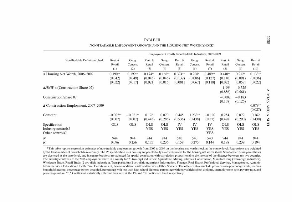
The right panel of Figure 1 repeats the exercise using the second definitionof non-tradable based on the geographical concentration of each four-digitindustry. While the set of industries defined as non-tradable under the seconddefinition is quite distinct from those defined as non-tradable under the firstdefinition, the results are remarkably similar.7 Columns 1 and 2 of Table IIIreport regressions of the change in non-tradable employment using the twodefinitions of non-tradable employment on change in housing net worth. Thecorrelation documented in Figure 1 is strong and significant at the 1% level.

All standard errors in this paper are clustered at the state level to allow forspatial correlation across counties within a state, and to allow for correlationwithin a state due to state-specific foreclosure, bankruptcy, or other labor mar-ket laws. We also report standard errors (in square brackets) that allow for spa-tial correlation among counties irrespective of state. In particular, we computethe distance between all county-pairs and allow for county-pairs to have a cor-relation that varies inversely with the distance between them. State-clusteredstandard errors tend to be larger and we report these standard errors in therest of the paper.

2.2. Supply-Side Sector-Specific Shocks

One concern with columns 1 and 2 is that the �HNW i may be spuriously cor-related with supply-side industry-specific shocks that impact both employmentand housing net worth. In particular, certain industries may be harder hit dur-ing the recession, and counties with greater exposure to these industries maynaturally experience both a larger decline in housing net worth and larger fallin employment.

We control for such supply-side sector-specific concerns in columns 3 and 4by including the share of a county’s employment in 2006 that is in each of the23 two-digit industries. There are therefore 23 additional control variables thatallow for separate industry effects for industries such as agriculture, mining,utilities, construction, wholesale trade, retail trade, finance, real estate, con-struction, and health care.8

The results show that the coefficient on the housing net worth shock doesnot change in any statistically significant sense, despite the fact that the R2

increases significantly. In the Supplemental Material, we use this informationto also conduct an omitted variable bias test as suggested by Oster (2014) basedon the work of Altonji, Elder, and Taber (2005).

7For visual clarity, we exclude some outlier counties with large decline in housing net worth(below −0�3). However, all these counties are included in the regression analysis and hence arenot excluded from our formal analysis.

8Table III lists all of the 23 two-digit industries.

2208A

.MIA

NA

ND

A.SU

FI

TABLE III

NON-TRADABLE EMPLOYMENT GROWTH AND THE HOUSING NET WORTH SHOCKa

Employment Growth, Non-Tradable Industries, 2007–2009

Non-Tradable Definition Used: Rest. & Geog. Rest. & Geog. Rest. & Geog. Rest. & Rest. & Geog. Rest. &Retail Concen. Retail Concen. Retail Concen. Retail Retail Concen. Retail

(1) (2) (3) (4) (5) (6) (7) (8) (9) (10)

� Housing Net Worth, 2006–2009 0�190∗∗ 0�199∗∗ 0�174∗∗ 0�166∗∗ 0�374∗∗ 0�208∗ 0�489∗∗ 0�440∗∗ 0�212∗ 0�133∗∗

(0.042) (0.049) (0.043) (0.046) (0.132) (0.086) (0.127) (0.140) (0.091) (0.036)[0.022] [0.017] [0.021] [0.016] [0.081] [0.067] [0.118] [0.072] [0.057] [0.022]

�HNW ∗ (Construction Share 07) −1�99∗ −0�325(0.856) (0.561)

Construction Share 07 −0�082 −0�183(0.158) (0.126)

� Construction Employment, 2007–2009 0�079∗∗

(0.027)

Constant −0�022∗∗ −0�021∗∗ 0.176 0.070 0.445 1�233∗∗ −0�102 0.254 0.072 0.162(0.007) (0.007) (0.443) (0.286) (0.536) (0.438) (0.57) (0.428) (0.290) (0.430)

Specification OLS OLS OLS OLS IV IV IV OLS OLS OLSIndustry controls? YES YES YES YES YES YES YES YESOther controls? YES

N 944 944 944 944 540 540 540 944 944 944R2 0.096 0.156 0.175 0.236 0.158 0.275 0.144 0.188 0.239 0.194

aThis table reports regression estimates of non-tradable employment growth from 2007 to 2009 on the housing net worth shock at the county level. Regressions are weightedby the total number of households in a county. The IV specification uses housing supply elasticity as an instrument for the housing net worth shock. Standard errors in parenthesesare clustered at the state level, and in square brackets are adjusted for spatial correlation with correlation proportional to the inverse of the distance between any two counties.The industry controls are the 2006 employment share in a county for 23 two-digit industries: Agriculture, Mining, Utilities, Construction, Manufacturing (3 two-digit industries),Wholesale Trade, Retail Trade (2 two-digit industries), Transportation (2 two-digit industries), Information, Finance, Real Estate, Professional Services, Management, Adminis-trative Services, Education, Health Care, Entertainment, Accommodation and Food Services, Other Services. The other controls include pre-recession percentage white, medianhousehold income, percentage owner-occupied, percentage with less than high school diploma, percentage with only a high school diploma, unemployment rate, poverty rate, andpercentage urban. ∗∗�∗ Coefficient statistically different than zero at the 1% and 5% confidence level, respectively.

THE 2007–2009 DROP IN EMPLOYMENT 2209

The Great Recession was particularly harsh on the construction sector, andone may worry that places where house prices and hence housing net worthfell the most also had greater exposure to the construction sector. We conducta number of checks to test this concern.

Our first test uses the Saiz (2010) housing supply elasticity as an instrumentfor the change in housing net worth. Mian, Rao, and Sufi (2013) showed thatwhile the Saiz instrument is strongly correlated with �HNW i, it is not corre-lated with either the share of employment in construction sector in a county,or the growth in construction sector employment prior to 2007.

Columns 5 and 6 instrument �HNW i with housing supply elasticity. The IVcoefficients are stronger than their OLS counterpart, showing that our resultsare robust to construction sector concerns. The number of observations de-clines because the housing supply elasticity variable is not available for allcounties. In unreported regressions, we show that the increase in coefficientrelative to the OLS version is not driven by the smaller sample size.

The estimated coefficients in Table III are large. For example, the IV esti-mate in column 5 implies that going from the 90th to the 10th percentile ofchange in housing net worth distribution in the cross-section leads to a lossin non-tradable employment of 8.2%. As a comparison, non-tradable employ-ment declines by 12% when we move from the 90th to the 10th percentile.The elasticity of spending with respect to housing net worth is estimated to be0.77 in Mian, Rao, and Sufi (2013), which implies an elasticity of non-tradableemployment with respect to spending of 0.48.9

While the instrument is orthogonal to construction sector exposure, theremay be a concern that it is correlated with other county-level demographic at-tributes in a way that biases the IV estimate. We test for this concern by includ-ing a number of county-level control variables in column 7, including percent-age white, median household income, percentage owner-occupied, percentagewith less than high school diploma, percentage with only a high school diploma,unemployment rate, poverty rate, and percentage urban. The coefficient of in-terest remains materially unchanged.

An alternative test for the concern regarding the construction sector is pre-sented in columns 8 and 9 that interact �HNW i with the share of employmentin the construction sector in 2007. The coefficient on the un-interacted �HNW i

reflects the (out of sample) predicted impact of �HNW i on the change in non-tradable employment for counties with zero construction sector exposure. Thispredicted impact remains strong and significant.

Column 10 explicitly controls for job losses in construction between 2007and 2009. It is an extreme test because including the change in constructionemployment on the right hand side is likely to “over control”: the spending

9The calculation of moving from 10th to 90th percentile is based on the IV sample with 540counties. Elasticity of spending is from Table III, column 4 of Mian, Rao, and Sufi (2013), and0�48 = 0�37/0�77.

2210 A. MIAN AND A. SUFI

response to the housing net worth decline will impact the construction sector aswell. Nonetheless, column 10 shows that the coefficient on change in housingnet worth remains positive and statistically significant at the 1% confidencelevel.

2.3. The Business Uncertainty Hypothesis

We next consider if the effect of the housing net worth shock on non-tradableemployment can be explained by the business uncertainty hypothesis, or theidea that policy or other government-induced uncertainty is responsible forthe decline in the economy. The canonical argument, as illustrated by Bloom(2009), is that uncertainty causes firms to temporarily pause their investmentand hiring.10

In its most basic form, an increase in business uncertainty at the aggregatelevel does not explain the stark cross-sectional patterns in non-tradable em-ployment losses that we have documented above. If the business uncertaintyhypothesis were to qualify as an explanation for our results, it would have tobe the case that the increase in business uncertainty was somehow larger incounties that experienced a large decline in housing net worth.

Of course, if businesses face more uncertainty because of a large decline inlocal demand in these areas, then this is simply another manifestation of thehousing net worth channel. The alternative explanation must involve greateruncertainty in areas with large housing net worth decline for reasons otherthan the decline in local demand itself. For example, perhaps there is moreuncertainty regarding state government policies in states with severe housingproblems.

Appendix Figures 1 and 2 in the Supplemental Material present an ad-ditional test of the uncertainty hypothesis based on state-level survey datafrom the National Federation of Independent Businesses. They show that busi-ness owners’ concerns regarding regulation and government policy increasedsignificantly later than the decline in employment. Moreover, there is norelationship between the increase in concerns regarding government taxa-tion/regulation and change in housing net worth, or the change in employmentat the state level.

These results suggest that the uncertainty hypothesis is unlikely to be drivingour main result. There is additional evidence that further corroborates thisview. As we will see below, there is no correlation between the housing networth shock and the change in tradable employment in a county. If supply-sidedriven business uncertainty were responsible for high non-tradable job losses

10Also see Baker, Bloom, and Davis (2011), Bloom (2009), Bloom, Foetotto, and Jaimovich(2010), Fernandez-Villaverde, Guerron-Quintana, Kuester, and Rubio-Ramirez (2011), andGilchrist, Sim, and Zakrajsek (2010).

THE 2007–2009 DROP IN EMPLOYMENT 2211

in counties with large housing net worth decline, then we would have expectedthe same result for tradable sector job loss as well.

In the Supplemental Material, we also address one additional form of un-certainty suggested by Mericle, Shoag, and Veuger (2012). Governments instates with housing problems may need to cut expenditures dramatically, thusraising business uncertainty.11 However, we show that such state governmentcuts were concentrated in 2009 (Appendix Figure 3), much later than when joblosses started. Further, we can control directly for mid-year state budget cutsand our results are robust (Appendix Table II).

2.4. The Credit Supply Hypothesis

Another alternative explanation for the relation between the change in non-tradable employment and the housing net worth shock is based on the possi-bility that firms in counties with a larger decline in housing net worth face alarger decline in credit supply, forcing them to lay off workers. For example,firms using real estate as collateral for funding might experience a more severereduction in credit supply in counties harder hit by the decline in house prices.

While credit supply shocks can be important drivers of firm investment, sur-vey evidence from business owners presented in Appendix Figure 1 shows thatonly 3% of respondents report financing as their main problem in 2007. Fur-ther, there is no appreciable increase in the response rate as the recession un-folds. Instead, businesses start complaining about poor sales and governmentregulation at a significantly higher rate during the recession.

A second result that goes against the credit supply hypothesis is presented inthe next section where we show that the change in tradable sector employmentis not correlated with the housing net worth shock. If a reduction in credit sup-ply were making firms fire workers, we would expect the drop in employmentto take place in both tradable and non-tradable sectors.

Finally, one may argue that business credit supply shocks only affect non-tradable industries. We test whether the relationship between the change innon-tradable employment and housing net worth shocks is driven by credit sup-ply tightening in Table IV. County business pattern data break down county-level employment in each four-digit industry further by the size of the under-lying reporting establishment. If our main result were driven by credit supplytightening, then we would expect the result to be stronger among smaller es-tablishments that are more likely to be credit-constrained.

Panel A splits the change in non-tradable employment by establishment sizeand regresses it on the change in housing net worth. Panel B repeats this exer-cise using the IV specification. If differential credit supply shocks in countieswith a large decline in housing net worth were driving our results, we wouldexpect our effect to be stronger for smaller establishments. Instead we find

11We are grateful to Daniel Shoag for highlighting this issue and providing data.

2212A

.MIA

NA

ND

A.SU

FI

TABLE IV

IS NON-TRADABLE EMPLOYMENT GROWTH DRIVEN BY CREDIT SUPPLY TIGHTENING?a

(1) (2) (3) (4) (5) (6)

Panel A (OLS): Effect of change in housing net worth on non-tradable employment growth by establishment size (N = 944 counties)

Establishment Size in Terms of Number of Employees:

1 to 4 5 to 9 10 to 19 20 to 49 50 to 99 100+� Housing Net Worth, 0�070∗∗ 0.032 0.022 0�134∗∗ 0.152 0�434∗∗

2006–2009 (0.025) (0.036) (0.044) (0.032) (0.097) (0.061)

Panel B (IV): Effect of change in housing net worth on non-tradable employment growth by establishment size (N = 540 counties)

Establishment Size in Terms of Number of Employees:

1 to 4 1 to 4 1 to 4 1 to 4 1 to 4 1 to 4

� Housing Net Worth, −0.134 0.000 −0.022 0�193∗ 0.335 0�770∗∗

2006–2009 (0.147) (0.125) (0.109) (0.086) (0.191) (0.208)

Panel C: Effect of change in housing net worth on non-tradable employment growth by banking type

Banking Type:

National Local National Local(OLS, N = 472) (OLS, N = 304) (IV, N = 472) (IV, N = 236)

� Housing Net Worth, 0�186∗∗ 0.306 0�233∗∗ 0�308∗∗

2006–2009 (0.041) (0.178) (0.068) (0.107)aThis table reports regression estimates of non-tradable employment growth from 2007 to 2009 on the housing net worth shock at the county level. Panels A and B reports the

OLS and IV coefficient estimates, respectively, for establishments of varying sizes. Panel C reports the coefficients separately for national and local banking markets. Non-tradableemployment is defined as employment in restaurant and retail industries at the four-digit industry level and then aggregated up separately for each county. All regressions areweighted using the total number of households in a county as weights. The instrumental variables specifications use the housing supply elasticity as an instrument for the change inhousing net worth in the first stage. Standard errors are clustered at the state level. ∗∗�∗ Coefficient statistically different than zero at the 1% and 5% confidence level, respectively.

THE 2007–2009 DROP IN EMPLOYMENT 2213

completely the opposite. Larger firms in hard hit counties see a larger decline.This is inconsistent with the credit supply view.

Panel C performs a different test of the credit supply hypothesis. It splits oursample into counties that are primarily served by national banks, and coun-ties that are largely served by local banks. Using the summary of deposits datafrom the FDIC, for every bank, we calculate the share of deposits of that bankin every county. Then, for every county, we average this statistic over the bankslocated in the county.12 A county that has banks that have a very low fractionof their deposits in that county is considered a national banking county. Theytherefore should not be as sensitive to local credit supply conditions. However,we find that the same pattern between non-tradable employment growth andhousing net worth change holds within both national and local banking coun-ties.

3. UNDERSTANDING THE ADJUSTMENT MECHANISMS: THEORY

The decline in county-level non-tradable employment in response to the de-cline in housing net worth potentially represents a partial equilibrium responseof the local labor market. The overall impact of these shocks depends on gen-eral equilibrium adjustments. For example, if wages are flexible and searchfrictions minimal, a negative shock to non-tradable employment might be com-pensated by a fall in local wages and increased employment in the tradablesector.

If such adjustment mechanisms are strong enough, the negative impact doc-umented above might not be important for the aggregate employment picture.On the other hand, the presence of real and nominal rigidities can make theeffect of the housing net worth shock more durable. We discuss the possibleadjustment mechanisms through the lens of a simple model.

3.1. Baseline Model

Consider an economy made up of S equally sized counties or “islands” in-dexed by c. Each county produces two types of goods, tradable (T ) and non-tradable (N). Counties can freely trade the tradable good, but must consumethe non-tradable good produced in their own county. We impose the restric-tion that labor cannot move across islands but can move freely between thetradable and non-tradable sectors within an island.

Each island has Dc units of total (nominal) consumer demand. Consumershave Cobb–Douglas preferences over the two consumption goods, and spendconsumption shares PN

c CNc = αDc and PTCT

c = (1 − α)Dc on the non-tradableand tradable good, respectively.

12We weight this average by the amount of deposits the bank has in the county.

2214 A. MIAN AND A. SUFI

All islands face the same tradable good price, while the non-tradable goodprice may be county-specific since each county must consume its own produc-tion of the non-tradable good. Production is governed by a constant returnstechnology for tradable and non-tradable goods with labor (e) as the only fac-tor input and produces output according to yT

c = beTc , and yNc = aeNc , respec-

tively.Total employment on each island is normalized to 1 with eTc + eNc = 1. Wages

in the non-tradable and tradable sectors are given by wNc = aPN

c and wTc =

bPT , respectively. Free mobility of labor across sectors equates the two wages,making the non-tradable good price independent of its county, that is, PN

c =baPT . Goods market equilibrium in non-tradable and tradable sectors implies

that yNc = CN

c on each island and∑S

c=1 ySc = ∑S

c=1 CTc .

We first solve the model under the symmetry assumption that, in the initialsteady state, all islands have the same nominal demand Dc = D0. Solving foroutput, employment, and prices, and denoting the initial steady state by super-script (∗), we obtain

e∗Nc = α� e∗T

c = (1 − α)� P∗Nc = D0

a�

P∗Tc = D0

b� w∗N

c = w∗Tc =D0�

The model is “money neutral” with nominal shocks translating one for oneinto prices and wages. Real allocation across islands remains unchanged inresponse to the shock, with employment in non-tradable and tradable sectorsgiven by α and (1 − α), respectively.

We next consider what happens if counties are hit with differing householdexpenditure shocks driven by the shocks to housing net worth discussed above.We normalize the initial nominal demand D0 = 1 and introduce the possibilityof negative demand shocks (δc) that differ across counties such that Dc = 1 −δc .13 Without loss of generality, we index counties such that δc+1 > δc and theaverage of the demand shocks is δ.

With the introduction of county-specific demand shocks, there are two dif-ferent scenarios to consider: one without nominal or real rigidities and anotherwith rigidities.

3.2. No Nominal or Real Rigidity

Suppose prices and wages are perfectly flexible (no nominal rigidity), andthere are no search or other frictions for labor to switch sectors (no real rigid-ity). Then there is deflation in response to negative demand shocks and an

13Both Eggertsson and Krugman (2012) and Guerrieri and Lorenzoni (2011) modeled thedemand shock as a tightening of the borrowing constraint on levered households who respond byreducing consumption.

THE 2007–2009 DROP IN EMPLOYMENT 2215

expansion in the tradable sector in certain counties. As we show in the Supple-mental Material, the change in prices and wages in the flexible price equilib-rium is given by �PT

c = − δb, �PN

c = − δa, �wN

c = �wTc = −δ.

The downward adjustment in prices and wages allows the economy to remainat full employment after the shock, with the change in non-tradable and trad-able employment in each county given by �eNc = −α(δc−δ

1−δ), and �eTc = α(δc−δ

1−δ).

As a result, counties with more negative demand shocks see a larger decline innon-tradable employment, which is completely compensated by an equivalentincrease in tradable employment in these counties.14

3.3. Full Nominal or Real Rigidity

Suppose instead that prices and wages are fully rigid, fixed at their initialsteady state level of P∗N

c , P∗Tc , w∗N

c , and w∗Tc . With fixed prices, the goods and la-

bor markets become “demand constrained” as in Hall (2011) and Bils, Klenow,and Malin (2013). Output and employment in the non-tradable sector is thengoverned by the new local demand for non-tradable goods at old steady stateprices, giving us eNc = α(1 − δc).

Output and employment in the tradable sector, however, depend on the av-erage demand for tradable goods across all islands, giving us eTc = (1 − α) ×(1 − δ). Let YN

c = −�eNc and YTc = −�eTc denote total employment loss in

county c in the non-tradable and tradable sectors, respectively. Then total em-ployment loss, Yc = YN

c +YTc , can be written as

Yc = αδc + (1 − α)δ�

With nominal rigidity, job losses in a county have a non-tradable componentthat depends only on the county-specific household expenditure shock, anda tradable component that depends on the overall expenditure shock hittingthe entire economy. Recall that under flexible prices, tradable employmentincreases in high δc counties, thereby compensating for jobs lost in the non-tradable sector in these counties. However, under price rigidity, there is nosuch adjustment in the tradable sector, generating zero correlation betweentradable employment growth and δc .

We would obtain a similar result if, instead of nominal rigidity, we introducedreal rigidity, or the assumption that workers cannot easily switch from non-tradable to tradable sector jobs. However, allowing for labor mobility acrossislands will tend to reduce the dispersion across islands in labor market out-comes. We will therefore test in the empirical section if labor systematicallymigrates from highly impacted counties to less impacted counties.

14This solution holds under the assumption that there are no corner solutions in any island,that is, α (1−δc)

(1−δ)= eNc ≤ 1, which translates into δ1 ≥ δ−(1−α)

α. See Supplemental Material for full

details.

2216 A. MIAN AND A. SUFI

4. UNDERSTANDING THE ADJUSTMENT MECHANISMS: EMPIRICS

4.1. Housing Net Worth Shock and Tradable Sector Employment

With flexible prices, the negative impact of the housing net worth shock onnon-tradable employment is reversed by a gain in employment in the tradablesector. The top two panels in Figure 2 test this by plotting the change in trad-able employment against the change in housing net worth across counties. Thetop-left panel uses the first definition of tradable employment based on indus-tries that are traded internationally, while the top-right panel uses the seconddefinition based on geographical concentration of industries. Despite the factthat the two definitions have many non-overlapping industries, there is no ev-idence of gain in tradable employment in counties that experience a largerdecline in housing net worth.

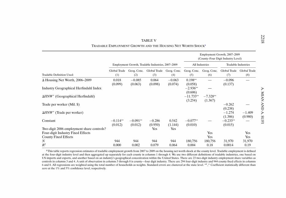
Columns 1 and 2 of Table V report regressions of tradable employmentgrowth in a county, using both definitions of “tradable,” on the housing networth shock. The estimated coefficients are close to zero and precisely es-timated. The difference between the coefficients for tradable job losses incolumns 1 and 2 of Table V and those for non-tradable job losses in columns1 and 2 of Table III are also statistically significant at the 1% level. Columns 3and 4 add the share of employment in each of 23 two-digit industries in 2006to control for differences in industry exposure across counties. The housingnet worth shock coefficient estimate is materially unchanged. The constants incolumns 1 and 2 are negative and large, implying that tradable sector employ-ment declines uniformly regardless of the size of the local housing net worthshock.

Column 5 uses data at the county-industry level and interacts the changein housing net worth with the industry-specific geographical Herfindahl indexlisted in Appendix Table I in the Supplemental Material. The specification usesa continuous definition of tradability for all industries to test whether the effectof housing net worth shock is stronger for more non-tradable industries. Eachcounty-industry observation is weighted by the total employment in that cell in2007.

The estimated coefficient on the change in housing net worth shock is pos-itive and significant, implying that job losses in the least concentrated (mostnon-tradable) industries are more severe in counties with a large housing networth decline. The interaction term is negative and significant, implying thatthe effect of housing net worth diminishes as industries become more geo-graphically concentrated. The implied effect of the housing net worth shockon employment for an industry at the 90th percentile of geographical concen-tration is 0.031 with standard error of 0.062, and it is −0�055 with a standarderror of 0.076 at the 95th percentile. The standard errors are computed usingthe Delta method. While the effect of the housing net worth shock on em-ployment gets close to zero for industries with a high degree of geographical

THE 2007–2009 DROP IN EMPLOYMENT 2217

FIGURE 2.—Tradable employment, wages, labor mobility, and the housing net worth shock.The top panel presents scatter-plots of county-level tradable employment growth from 2007Q1to 2009Q1 against the change in housing net worth from 2006 to 2009. The top-left panel definesindustries as tradable if they appear in U.S. global trade, and the top-right panel defines industriesas tradable if they are geographically concentrated in the United States. The middle panels plotwage growth (using payroll data) and hourly wage growth (using ACS data) against the change inhousing net worth. The bottom panel plots population growth and labor force growth against thechange in housing net worth. The sample includes counties with more than 50,000 households.

2218A

.MIA

NA

ND

A.SU

FI

TABLE V

TRADABLE EMPLOYMENT GROWTH AND THE HOUSING NET WORTH SHOCKa

Employment Growth, 2007–2009(County–Four Digit Industry Level)

Employment Growth, Tradable Industries, 2007–2009 All Industries Tradable Industries

Global Trade Geog. Conc. Global Trade Geog. Conc. Geog. Conc. Geog. Conc. Global Trade Global TradeTradable Definition Used: (1) (2) (3) (4) (5) (6) (7) (8)

� Housing Net Worth, 2006–2009 0.018 −0�085 0.064 −0�063 0�198∗∗ — −0�096 —(0.099) (0.063) (0.098) (0.074) (0.058) (0.137)

Industry Geographical Herfindahl Index −2�936∗∗ —(0.606)

�HNW ∗ (Geographical Herfindahl) −11�733∗∗ −7�328∗∗

(3.254) (1.367)Trade per worker (Mil. $) −0�262 —

(0.238)�HNW ∗ (Trade per worker) −1�274 −1�409

(1.386) (0.980)Constant −0�114∗∗ −0�091∗∗ −0�286 0.542 −0�077∗∗ — −0�233∗∗ —

(0.012) (0.012) (0.950) (1.144) (0.010) (0.015)Two-digit 2006 employment share controls? Yes YesFour-digit Industry Fixed Effects Yes YesCounty Fixed Effects Yes YesN 944 944 944 944 180,756 180,756 31,970 31,970R2 0.000 0.002 0.079 0.064 0.004 0.18 0.0014 0.19

aThis table reports regression estimates of tradable employment growth from 2007 to 2009 on the housing net worth shock at the county level. Tradable employment is definedat the four-digit industry level and then aggregated up separately for each county in columns 1 through 4. We use two different definitions of tradable industries, one based onUS imports and exports, and another based on an industry’s geographical concentration within the United States. There are 23 two-digit industry employment share variables ascontrols in columns 3 and 4. A unit of observation in columns 5 through 8 is county—four digit industry. There are 294 four-digit industry and 944 county fixed effects in columns6 and 8. All regressions are weighted using the total number of households as weights. Standard errors are clustered at the state level. ∗∗�∗ Coefficient statistically different thanzero at the 1% and 5% confidence level, respectively.

THE 2007–2009 DROP IN EMPLOYMENT 2219

concentration (i.e., the most tradable industries), it does not turn significantlynegative.15

Column 6 adds four-digit industry fixed effects (294 industries) and countyfixed effects (944 counties). The industry fixed effects force comparison to bemade within the same four-digit industry across counties. Such fixed effectstherefore control for aggregate shifts at the industry level during the 2007–2009 period. The county fixed effects nonparametrically take out any county-specific changes over 2007–2009. Despite the inclusion of these fixed effects,our key result remains unchanged: the effect of the housing net worth shockon employment is stronger for non-tradable industries that are geographicallyleast concentrated across the United States.

The regressions reported in columns 7 and 8 restrict sample to industries de-fined as tradable according to global trade and interact the change in housingnet worth with the level of trade per worker in an industry. The interactionterms are not significant, showing that the effect of housing net worth on em-ployment does not vary within the tradable sector.

4.2. Housing Net Worth Shock, Wage Flexibility, and Labor Mobility

Columns 1 and 2 of Table VI and the middle-left panel of Figure 2 usecounty-level data on payroll wage growth to show that counties with large de-cline in housing net worth experience a small relative decline in payroll wagegrowth from 2007 to 2009. However, the coefficient is small in magnitude andstatistically significant only with two-digit industry controls.16

Payroll wage growth also includes changes in the number of hours workedthat could differentially affect counties with a greater decline in housing networth. In columns 3 and 4 and the middle-right panel of Figure 2, we use hourlywage growth as the dependent variable, which shows no strong relation withthe housing net worth shock.

Following Blanchard and Katz (1992), we also evaluate mobility. Thebottom-left panel of Figure 2 and columns 5 and 6 of Table VI correlatecounty-level population growth from 2007 to 2009 with the change in hous-ing net worth. While population growth is uncorrelated with the change inhousing net worth by itself, the correlation turns significant with two-digit in-dustry share controls (column 6). However, this result is not robust to alter-native definitions of mobility. Columns 7 and 8 use the American CommunitySurvey data on propensity of respondents to have migrated into their current

15It is only at the extreme end of the tradability distribution that the effect of housing networth becomes negative and significant. For example, at the 99th percentile, the effect is −0�48with standard error of 0.18.

16There are a number of other papers independently arguing for the presence of price andwage rigidities in the Great Recession, in particular, Daly, Hobijn, and Lucking (2012), Daly,Hobijn, and Wiles (2011), Fallick, Lettau, and Wascher (2011), and Hall (2011).

2220A

.MIA

NA

ND

A.SU

FI

TABLE VI

WAGES, MOBILITY, AND THE HOUSING NET WORTH SHOCKa

Total Wage Growth, Average Hourly Wage Growth, Population Growth, In-Migration Growth, Labor Force Growth,2007 to 2009, CBP 2007 to 2009, ACS 2007–2009 2007–2009 2007–2009

(1) (2) (3) (4) (5) (6) (7) (8) (9) (10)

� Housing Net Worth, 2006–2009 0.061 0�078∗ 0.054 0.056 0.019 0�057∗∗ −0�042 −0�128 −0�0094 0.0032(0.041) (0.037) (0.039) (0.035) (0.021) (0.021) (0.11) (0.127) (0.020) (0.024)

Constant 0�031∗∗ −0�325 0�037∗∗ 0.078 0�021∗∗ −0�103 −0�010∗∗ −0�530 0.0136 0.030(0.007) (0.250) (0.003) (0.20) (0.004) (0.137) (0.015) (1.778) (0.004) (0.24)

Two-digit 2006 employmentshare controls? Yes Yes Yes Yes Yes

N 944 944 943 943 939 939 943 943 944 944R2 0.012 0.16 0.018 0.076 0.009 0.25 0 0.027 0.001 0.12

aColumns 1 through 4 present coefficients from regressions relating wage growth in a county from 2007 to 2009 to the housing net worth shock. The specifications in columns1 and 2 use total wages from the Census County Business Patterns data, and columns 3 and 4 use hourly wage growth data from the American Community Survey. Columns5 through 10 present coefficients from regressions relating mobility and labor force participation in a county from 2007 to 2009 to the change in housing net worth. Columns5 and 6 use census data on population growth, columns 7 and 8 use growth in in-migration from the American Community Survey, and columns 9 and 10 use labor force growthfrom the Bureau of Labor Statistics. All regressions are weighted using the total number of households in a county as weights. Standard errors are clustered at the state level.∗∗�∗ Coefficient statistically different than zero at the 1% and 5% confidence level, respectively.

THE 2007–2009 DROP IN EMPLOYMENT 2221

county of residence. There is no evidence that in-migration growth is faster incounties that are less negatively impacted by the housing net worth shock. Fur-ther support for this result is provided by Yagan (2014), who used geo-codedindividual-level data from tax returns to show that individuals experiencingnegative employment shocks were not able to insure against these shocks bymoving to areas with lower unemployment rates.

Finally, the bottom-right panel of Figure 2 and columns 9 and 10 correlatelabor force growth with the change in housing net worth and show there is noclear relationship. Overall, the results in Figure 2 and Table VI show that themigration of workers from counties with a large decline in housing net worthto counties with smaller declines is unlikely to explain the drop in non-tradableemployment in counties with a large decline in housing net worth.

5. CONCLUSION

The Great Recession resulted in a remarkable loss of jobs between 2007 and2009. This paper outlines the importance of the housing net worth shock andshows that housing net worth losses led to significant non-tradable sector joblosses in the cross-section. This result is not driven by supply-side industry-specific shocks (such as construction) or credit supply conditions. We also donot find strong evidence of labor market adjustment through wages, labor mo-bility, or expansion in tradable employment in harder hit counties.

Our results are robust to two distinct definitions of non-tradable and trad-able sectors. Our second definition of non-tradable and tradable sectors, basedon the geographical concentration of each four-digit industry, is new to the lit-erature and can be used more generally in empirical studies exploiting regionalor international shocks.

An important question for future research concerns the effect of the hous-ing boom on employment. Our study uses the collapse in housing net worthas its starting point. However, the housing boom itself may have affected em-ployment patterns before the recession, and as such the job losses that we doc-ument may represent the return to more “normal” housing conditions. Forexample, Charles, Hurst, and Notowidigo (2012) argued that the positive em-ployment effects of the housing boom masked the broader fall in employmentdue to a decline in manufacturing.

Another question for future research is about the persistence of high lev-els of unemployment beyond 2009. A recent paper by Hagedorn, Karahan,Manovskii, and Mitman (2013) argued that unemployment benefit extensionsexplain a large part of the persistently high level of unemployment after 2009.In another paper, Jaimovich and Siu (2013) argued that the automation ofroutine tasks over time leads to job polarization in the face of a sudden down-turn. This generates “jobless recoveries” where the fall in employment in non-routine employment is more permanent. Understanding the longer term de-cline in employment to population ratio remains a very important question forfurther investigation.

2222 A. MIAN AND A. SUFI

REFERENCES

ALTONJI, J., T. ELDER, AND C. TABER (2005): “Selection on Observed and Unobserved Vari-ables: Assessing the Effectiveness of Catholic Schools,” Journal of Political Economy, 113 (1),151–184. [2207]

BAKER, S., N. BLOOM, AND S. DAVIS (2011): “Measuring Economic Policy Uncertainty,” WorkingPaper, Chicago Booth. [2210]

BILS, M., P. KLENOW, AND B. MALIN (2013): “Testing for Keynesian Labor Demand,” in NBERMacroeconomics Annual. Chicago: University of Chicago Press, 311–349. [2199,2215]

BLANCHARD, O., AND L. KATZ (1992): “Regional Evolutions,” Brookings Papers on EconomicActivity, 1, 1–75. [2219]

BLOOM, N. (2009): “The Impact of Uncertainty Shocks,” Econometrica, 77, 623–685. [2210]BLOOM, N., M. FOETOTTO, AND N. JAIMOVICH (2010): “Really Uncertain Business Cycles,”

Working Paper, Stanford University. [2210]CHARLES, K. K., E. HURST, AND M. NOTOWIDIGO (2012): “Manufacturing Busts, Housing

Booms, and Declining Employment: A Structural Explanation,” Working Paper, Universityof Chicago. [2221]

DALY, M., B. HOBIJN, AND B. LUCKING (2012): “Why Has Wage Growth Stayed Strong?” FRBSFEconomic Letter, April 2, 2012. [2219]

DALY, M. C., B. HOBIJN, AND T. S. WILES (2011): “Aggregate Real Wages: Macro Fluctuationsand Micro Drivers,” Working Paper 2011-23, FRBSF. [2219]

EGGERTSSON, G., AND P. KRUGMAN (2012): “Debt, Deleveraging, and the Liquidity Trap:A Fisher–Minsky–Koo Approach,” Quarterly Journal of Economics, 127, 1469–1513. [2199,

2214]FALLICK, B., M. LETTAU, AND W. WASCHER (2011): “Downward Nominal Wage Rigidity in the

United States During the Great Recession,” Working Paper. [2219]FARHI, E., AND I. WERNING (2013): “A Theory of Macroprudential Policies in the Presence of

Nominal Rigidities,” Working Paper, MIT. [2199]FERNANDEZ-VILLAVERDE, J., P. A. GUERRON-QUINTANA, K. KUESTER, AND J. RUBIO-

RAMIREZ (2011): “Fiscal Uncertainty and Economic Activity,” Working Paper, University ofPennsylvania. [2210]

GILCHRIST, S., J. W. SIM, AND E. ZAKRAJSEK (2010): “Uncertainty, Financial Frictions, and In-vestment Dynamics,” Working Paper, Boston University. [2210]

GUERRIERI, V., AND G. LORENZONI (2011): “Credit Crises, Precautionary Savings, and the Liq-uidity Trap,” Working Paper, Chicago Booth. [2199,2214]

HAGEDORN, M., F. KARAHAN, I. MANOVSKII, AND K. MITMAN (2013): “Unemployment Bene-fits and Unemployment in the Great Recession: The Role of Macro Effects,” Working Paper19499, NBER. [2221]

HALL, R. E. (2011): “The Long Slump,” American Economic Review, 101, 431–469. [2199,2215,2219]

JAIMOVICH, N., AND H. SIU (2013): “The Trend Is the Cycle: Job Polarization and Jobless Recov-eries,” Working Paper. [2221]

MERICLE, D., D. SHOAG, AND S. VEUGER (2012): “Uncertainty and the Geography of the GreatRecession,” Working Paper, HKS. [2211]

MIAN, A., AND A. SUFI (2014): “Supplement to ‘What Explains the 2007–2009 Drop in Employ-ment?’,” Econometrica Supplemental Material, 82, http://dx.doi.org/10.3982/ECTA10451. [2201]

MIAN, A., K. RAO, AND A. SUFI (2013): “Household Balance Sheets, Consumption, and the Eco-nomic Slump,” Quarterly Journal of Economics, 128, 1687–1726. [2197,2198,2200,2205,2209]

MIDRIGAN, V., AND T. PHILIPPON (2011): “Household Leverage and the Recession,” WorkingPaper, NYU Stern. [2199]

OSTER, E. (2014): “Unobservable Selection and Coefficient Stability: Theory and Evidence,”Working Paper, Chicago Booth. [2207]

THE 2007–2009 DROP IN EMPLOYMENT 2223

SAIZ, A. (2010): “The Geographic Determinants of Housing Supply,” Quarterly Journal of Eco-nomics, 125, 1253–1296. [2209]

STUMPNER, S. (2013): “Trade and the Geographic Spread of the Great Recession,” WorkingPaper, U.C. Berkeley. [2199]

YAGAN, D. (2014): “Moving to Opportunity? Migratory Insurance Over the Great Recession,”Working Paper, U.C. Berkeley. [2221]

Princeton University, 26 Prospect Avenue, Princeton, NJ 08540, U.S.A. andNBER; atif@princeton.edu

andUniversity of Chicago Booth School of Business, 5807 S. Woodlawn Avenue,

Chicago, IL 60637, U.S.A. and NBER; amir.sufi@chicagobooth.edu.

Manuscript received November, 2011; final revision received July, 2014.