Embed Size (px)
Citation preview

Dr. Shalabh Department of Mathematics and Statistics
Indian Institute of Technology Kanpur
ECONOMETRIC THEORY
MODULE – XIX
Lecture - 45
Exercises

Exercise 1 The following data has been obtained on 26 days on the price of a share in the stock market and the daily change in the
stock market index. Now we illustrate the use of regression tools and the interpretation of the output from a statistical
software through this example.
2
Day no. (i) Change in index (Xi)
Value of share (yi) Day no. (i) Change in index (Xi)
Value of share (yi)
1 87 199 14 70 172
2 52 160 15 71 176
3 50 160 16 65 165
4 88 175 17 67 150
5 79 193 18 75 170
6 70 189 19 80 189
7 40 155 20 82 190
8 63 150 21 76 185
9 70 170 22 86 190
10 60 171 23 68 165
11 44 160 24 89 200
12 47 165 25 70 172
13 42 148 26 83 190
3
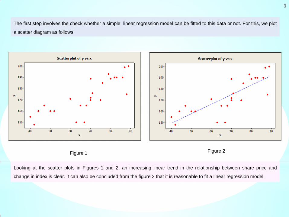
The first step involves the check whether a simple linear regression model can be fitted to this data or not. For this, we plot
a scatter diagram as follows:
Figure 1 Figure 2
Looking at the scatter plots in Figures 1 and 2, an increasing linear trend in the relationship between share price and
change in index is clear. It can also be concluded from the figure 2 that it is reasonable to fit a linear regression model.
4
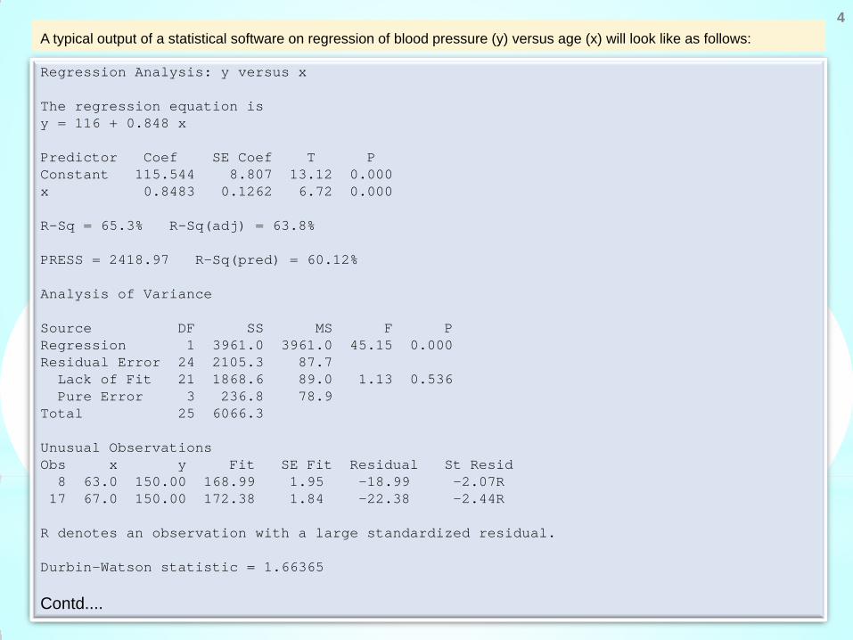
Regression Analysis: y versus x The regression equation is y = 116 + 0.848 x Predictor Coef SE Coef T P Constant 115.544 8.807 13.12 0.000 x 0.8483 0.1262 6.72 0.000 R-Sq = 65.3% R-Sq(adj) = 63.8% PRESS = 2418.97 R-Sq(pred) = 60.12% Analysis of Variance Source DF SS MS F P Regression 1 3961.0 3961.0 45.15 0.000 Residual Error 24 2105.3 87.7 Lack of Fit 21 1868.6 89.0 1.13 0.536 Pure Error 3 236.8 78.9 Total 25 6066.3 Unusual Observations Obs x y Fit SE Fit Residual St Resid 8 63.0 150.00 168.99 1.95 -18.99 -2.07R 17 67.0 150.00 172.38 1.84 -22.38 -2.44R R denotes an observation with a large standardized residual. Durbin-Watson statistic = 1.66365
Contd....
A typical output of a statistical software on regression of blood pressure (y) versus age (x) will look like as follows:
5
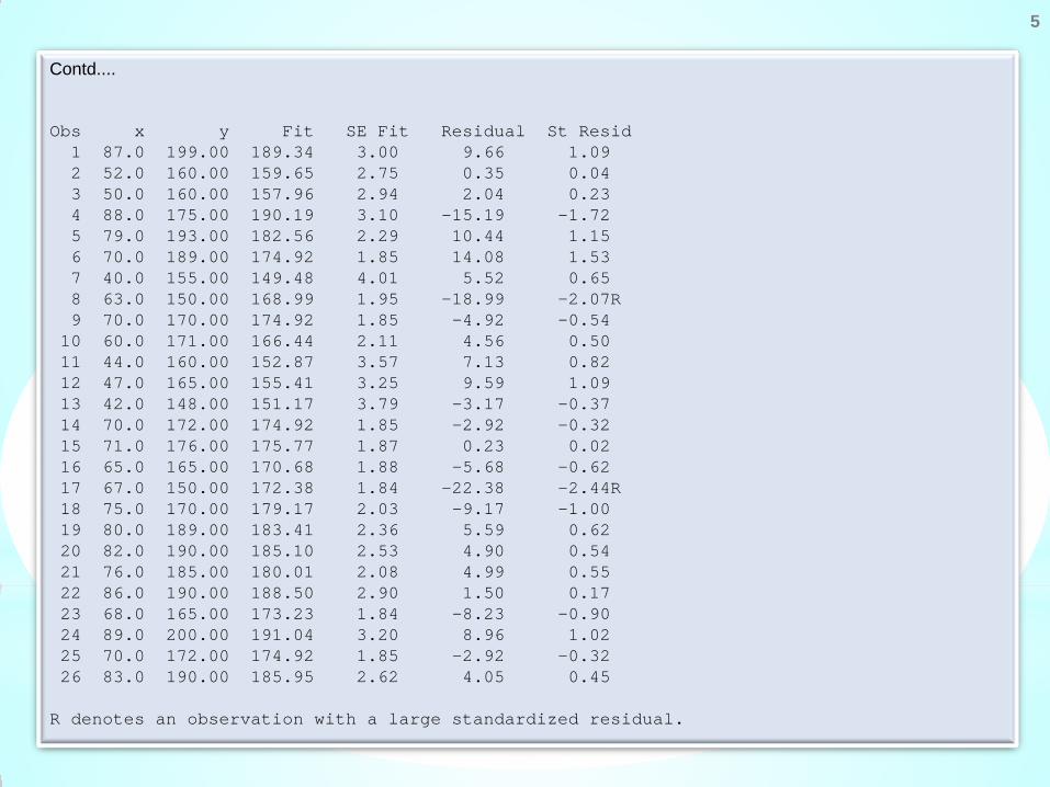
Contd.... Obs x y Fit SE Fit Residual St Resid 1 87.0 199.00 189.34 3.00 9.66 1.09 2 52.0 160.00 159.65 2.75 0.35 0.04 3 50.0 160.00 157.96 2.94 2.04 0.23 4 88.0 175.00 190.19 3.10 -15.19 -1.72 5 79.0 193.00 182.56 2.29 10.44 1.15 6 70.0 189.00 174.92 1.85 14.08 1.53 7 40.0 155.00 149.48 4.01 5.52 0.65 8 63.0 150.00 168.99 1.95 -18.99 -2.07R 9 70.0 170.00 174.92 1.85 -4.92 -0.54 10 60.0 171.00 166.44 2.11 4.56 0.50 11 44.0 160.00 152.87 3.57 7.13 0.82 12 47.0 165.00 155.41 3.25 9.59 1.09 13 42.0 148.00 151.17 3.79 -3.17 -0.37 14 70.0 172.00 174.92 1.85 -2.92 -0.32 15 71.0 176.00 175.77 1.87 0.23 0.02 16 65.0 165.00 170.68 1.88 -5.68 -0.62 17 67.0 150.00 172.38 1.84 -22.38 -2.44R 18 75.0 170.00 179.17 2.03 -9.17 -1.00 19 80.0 189.00 183.41 2.36 5.59 0.62 20 82.0 190.00 185.10 2.53 4.90 0.54 21 76.0 185.00 180.01 2.08 4.99 0.55 22 86.0 190.00 188.50 2.90 1.50 0.17 23 68.0 165.00 173.23 1.84 -8.23 -0.90 24 89.0 200.00 191.04 3.20 8.96 1.02 25 70.0 172.00 174.92 1.85 -2.92 -0.32 26 83.0 190.00 185.95 2.62 4.05 0.45 R denotes an observation with a large standardized residual.
5
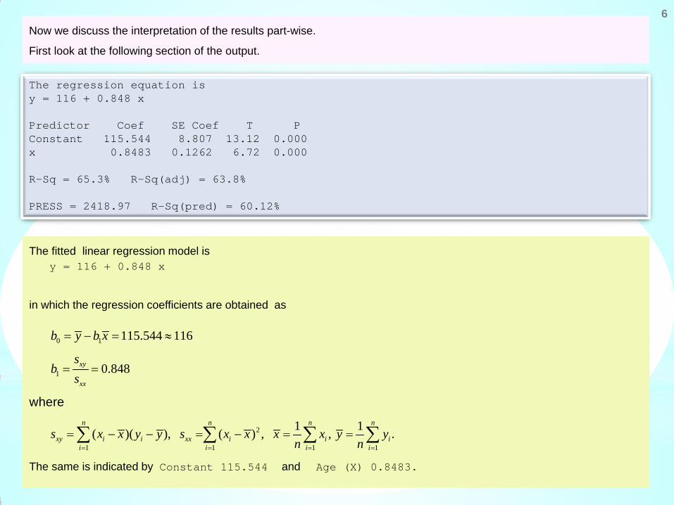
6 Now we discuss the interpretation of the results part-wise.
First look at the following section of the output.
The regression equation is y = 116 + 0.848 x Predictor Coef SE Coef T P Constant 115.544 8.807 13.12 0.000 x 0.8483 0.1262 6.72 0.000 R-Sq = 65.3% R-Sq(adj) = 63.8% PRESS = 2418.97 R-Sq(pred) = 60.12%
The fitted linear regression model is y = 116 + 0.848 x
in which the regression coefficients are obtained as
The same is indicated by Constant 115.544 and Age (X) 0.8483.
0 1
1
2
1 1 1 1
115.544 116
0.848
1 1( )( ), ( ) , , .
xy
xx
n n n n
xy i i xx i i ii i i i
b y b x
sb
s
s x x y y s x x x x y yn n= = = =
= − = ≈
= =
= − − = − = =∑ ∑ ∑ ∑
where
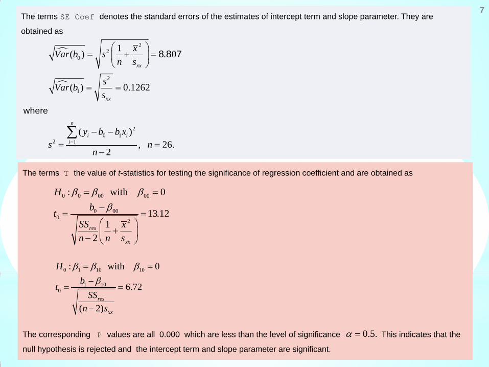
7 The terms SE Coef denotes the standard errors of the estimates of intercept term and slope parameter. They are
obtained as
22
0
2
1
20 1
2 1
1( ) . 0
( ) 0.1262
( ), 26.
2
where
8 8 7
xx
xx
n
i ii
xVar b sn s
sVar bs
y b b xs n
n=
= + =
= =
− −= =
−
∑
The terms T the value of t-statistics for testing the significance of regression coefficient and are obtained as
The corresponding P values are all 0.000 which are less than the level of significance This indicates that the
null hypothesis is rejected and the intercept term and slope parameter are significant.
0 0 00 00
0 000
2
: with 0
13.121
2res
xx
Hbt
SS xn n s
β β ββ
= =
−= =
+ −
0 1 10 10
1 100
: with 0
6.72
( 2)res
xx
Hbt
SSn s
β β ββ
= =−
= =
−
0.5.α =

8 Now we discuss the interpretation of the goodness of fit statistics.
The value of coefficient of determination is given by R-Sq = 65.3%.
This value is obtained from
2
2
1
'1 0.653.( )
n
ii
e eRy y
=
= − =−∑
The value of adjusted coefficient of determination is given by R-Sq(adj) = 63.8%.
This value is obtained from
This means that the fitted model can expalain about 64% of the variability in y through X.
2 211 (1 ) 0.638 1 with .nR R kn k− = − − = = −
9
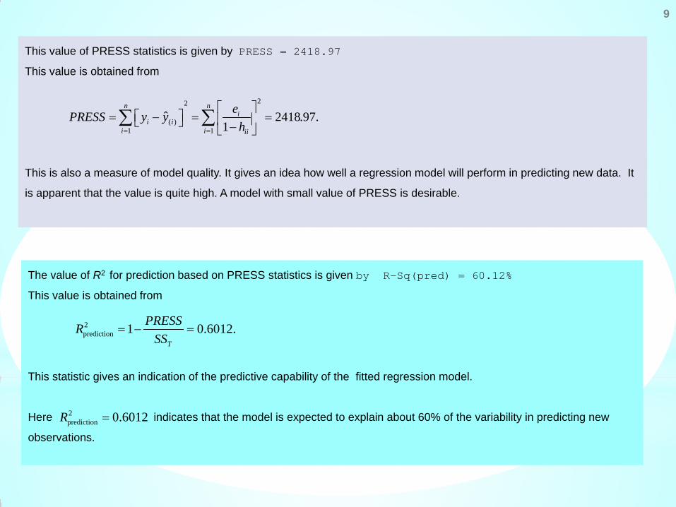
This value of PRESS statistics is given by PRESS = 2418.97
This value is obtained from
This is also a measure of model quality. It gives an idea how well a regression model will perform in predicting new data. It
is apparent that the value is quite high. A model with small value of PRESS is desirable.
22
( )1 1
ˆ 2418.97.1
n ni
i ii i ii
ePRESS y yh= =
= − = = −
∑ ∑
The value of R2 for prediction based on PRESS statistics is given by R-Sq(pred) = 60.12%
This value is obtained from
This statistic gives an indication of the predictive capability of the fitted regression model.
Here indicates that the model is expected to explain about 60% of the variability in predicting new
observations.
2prediction 1 0.6012.
T
PRESSRSS
= − =
2prediction 0.6012R =
10
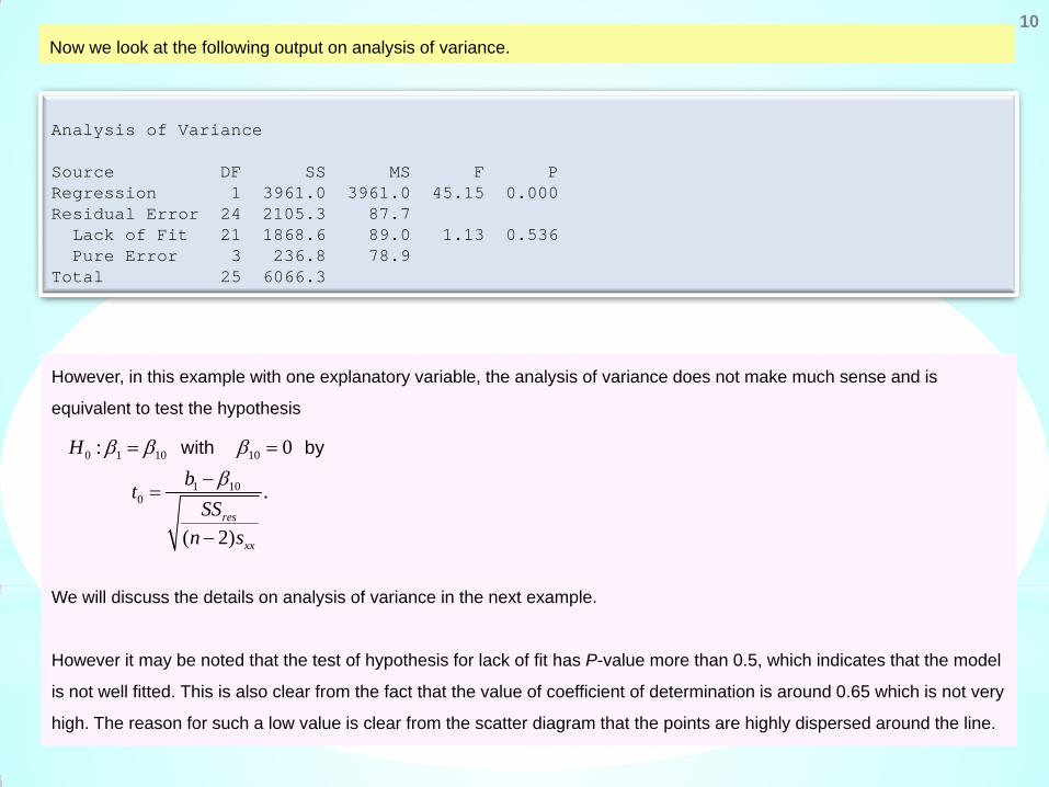
Analysis of Variance Source DF SS MS F P Regression 1 3961.0 3961.0 45.15 0.000 Residual Error 24 2105.3 87.7 Lack of Fit 21 1868.6 89.0 1.13 0.536 Pure Error 3 236.8 78.9 Total 25 6066.3
Now we look at the following output on analysis of variance.
However, in this example with one explanatory variable, the analysis of variance does not make much sense and is
equivalent to test the hypothesis
We will discuss the details on analysis of variance in the next example.
However it may be noted that the test of hypothesis for lack of fit has P-value more than 0.5, which indicates that the model
is not well fitted. This is also clear from the fact that the value of coefficient of determination is around 0.65 which is not very
high. The reason for such a low value is clear from the scatter diagram that the points are highly dispersed around the line.
0 1 10 10
1 100
: 0
.
( 2)
with by
res
xx
Hbt
SSn s
β β ββ
= =−
=
−
11
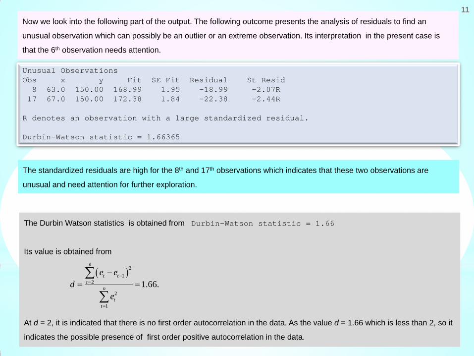
Unusual Observations Obs x y Fit SE Fit Residual St Resid 8 63.0 150.00 168.99 1.95 -18.99 -2.07R 17 67.0 150.00 172.38 1.84 -22.38 -2.44R R denotes an observation with a large standardized residual. Durbin-Watson statistic = 1.66365
Now we look into the following part of the output. The following outcome presents the analysis of residuals to find an
unusual observation which can possibly be an outlier or an extreme observation. Its interpretation in the present case is
that the 6th observation needs attention.
The Durbin Watson statistics is obtained from Durbin-Watson statistic = 1.66
Its value is obtained from
At d = 2, it is indicated that there is no first order autocorrelation in the data. As the value d = 1.66 which is less than 2, so it
indicates the possible presence of first order positive autocorrelation in the data.
( )21
2
2
1
1.66.
n
t tt
n
tt
e ed
e
−=
=
−= =∑
∑
The standardized residuals are high for the 8th and 17th observations which indicates that these two observations are
unusual and need attention for further exploration.
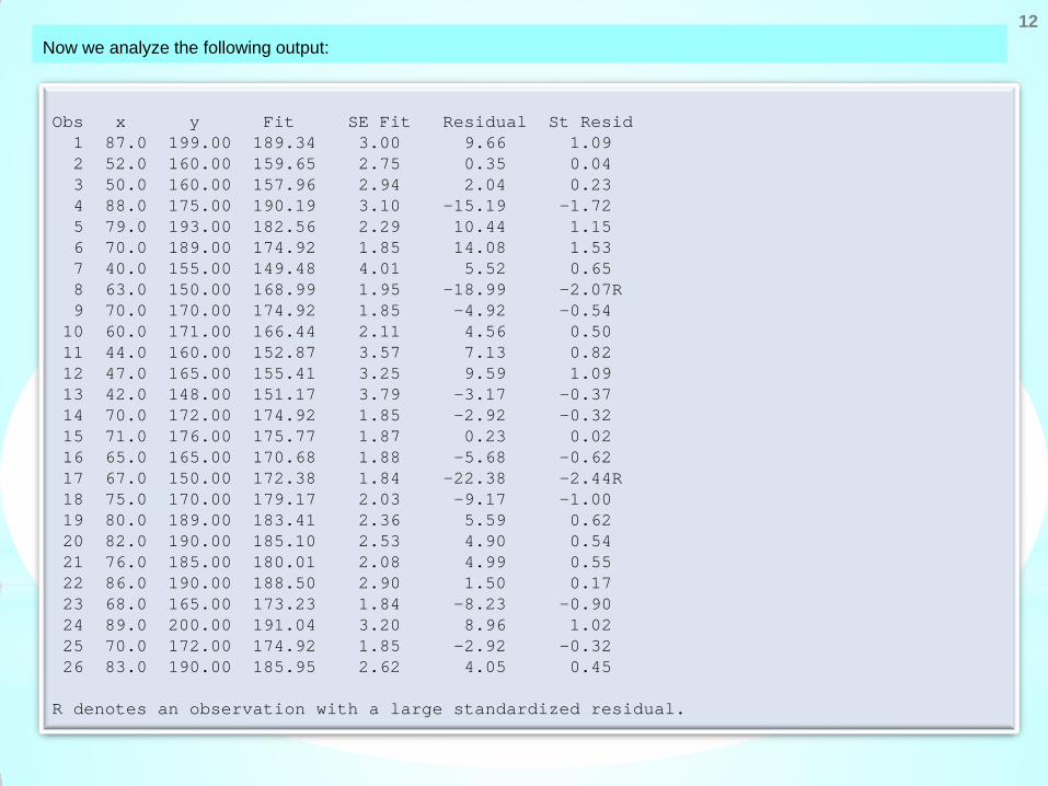
Obs x y Fit SE Fit Residual St Resid 1 87.0 199.00 189.34 3.00 9.66 1.09 2 52.0 160.00 159.65 2.75 0.35 0.04 3 50.0 160.00 157.96 2.94 2.04 0.23 4 88.0 175.00 190.19 3.10 -15.19 -1.72 5 79.0 193.00 182.56 2.29 10.44 1.15 6 70.0 189.00 174.92 1.85 14.08 1.53 7 40.0 155.00 149.48 4.01 5.52 0.65 8 63.0 150.00 168.99 1.95 -18.99 -2.07R 9 70.0 170.00 174.92 1.85 -4.92 -0.54 10 60.0 171.00 166.44 2.11 4.56 0.50 11 44.0 160.00 152.87 3.57 7.13 0.82 12 47.0 165.00 155.41 3.25 9.59 1.09 13 42.0 148.00 151.17 3.79 -3.17 -0.37 14 70.0 172.00 174.92 1.85 -2.92 -0.32 15 71.0 176.00 175.77 1.87 0.23 0.02 16 65.0 165.00 170.68 1.88 -5.68 -0.62 17 67.0 150.00 172.38 1.84 -22.38 -2.44R 18 75.0 170.00 179.17 2.03 -9.17 -1.00 19 80.0 189.00 183.41 2.36 5.59 0.62 20 82.0 190.00 185.10 2.53 4.90 0.54 21 76.0 185.00 180.01 2.08 4.99 0.55 22 86.0 190.00 188.50 2.90 1.50 0.17 23 68.0 165.00 173.23 1.84 -8.23 -0.90 24 89.0 200.00 191.04 3.20 8.96 1.02 25 70.0 172.00 174.92 1.85 -2.92 -0.32 26 83.0 190.00 185.95 2.62 4.05 0.45 R denotes an observation with a large standardized residual.
12 Now we analyze the following output:
13
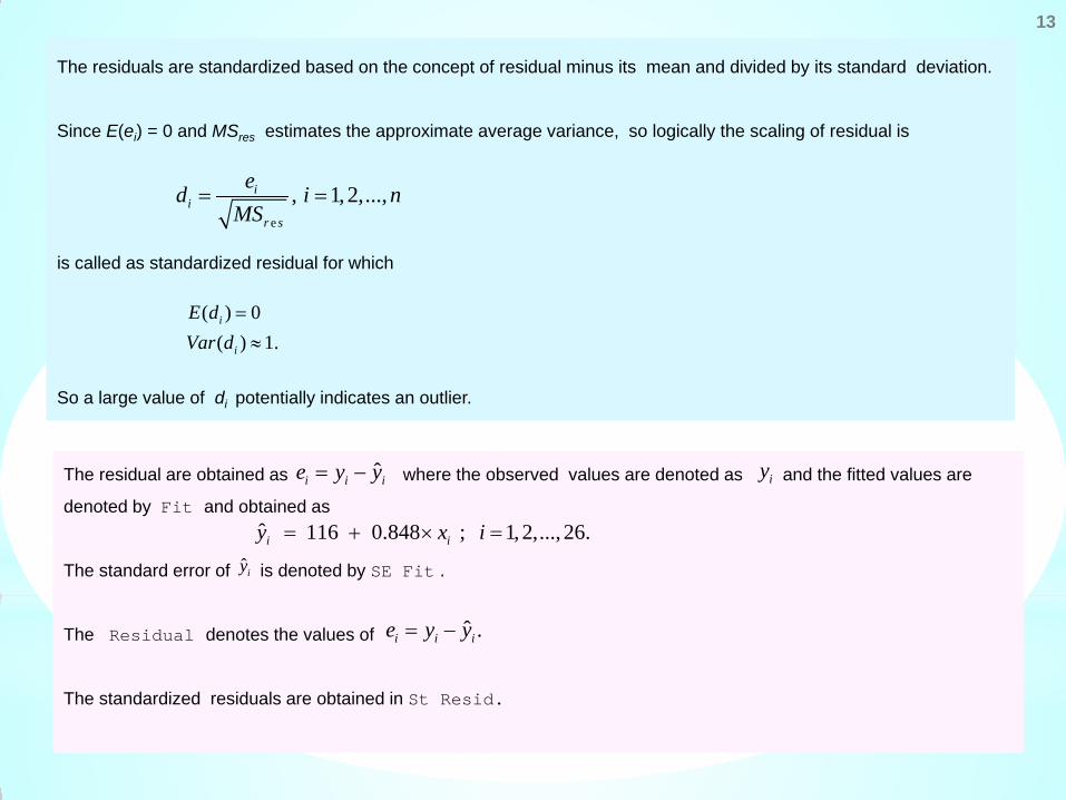
The residuals are standardized based on the concept of residual minus its mean and divided by its standard deviation.
Since E(ei) = 0 and MSres estimates the approximate average variance, so logically the scaling of residual is
is called as standardized residual for which
So a large value of di potentially indicates an outlier.
e
, 1, 2,...,ii
r s
ed i nMS
= =
( ) 0( ) 1.i
i
E dVar d
=
≈
The residual are obtained as where the observed values are denoted as and the fitted values are
denoted by Fit and obtained as
The standard error of is denoted by SE Fit .
The Residual denotes the values of
The standardized residuals are obtained in St Resid.
ˆi i ie y y= −
ˆ 116 0.848 ; 1, 2,..., 26.i iy x i= + × =
iy
ˆiy
ˆ .i i ie y y= −
14
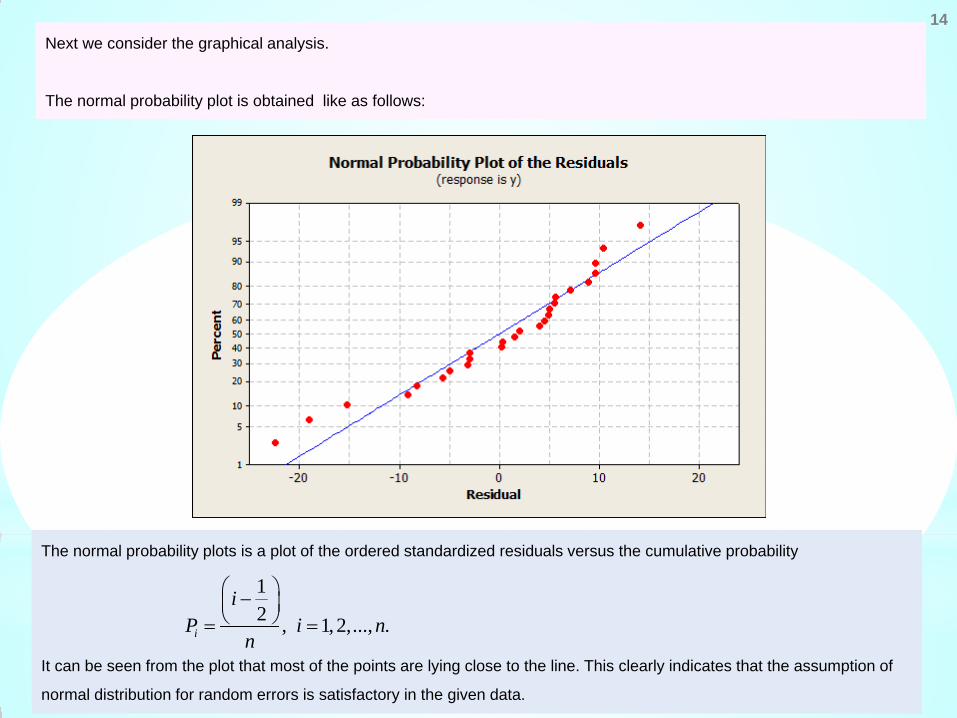
Next we consider the graphical analysis.
The normal probability plot is obtained like as follows:
The normal probability plots is a plot of the ordered standardized residuals versus the cumulative probability
It can be seen from the plot that most of the points are lying close to the line. This clearly indicates that the assumption of
normal distribution for random errors is satisfactory in the given data.
12 , 1,2,..., .i
iP i n
n
− = =
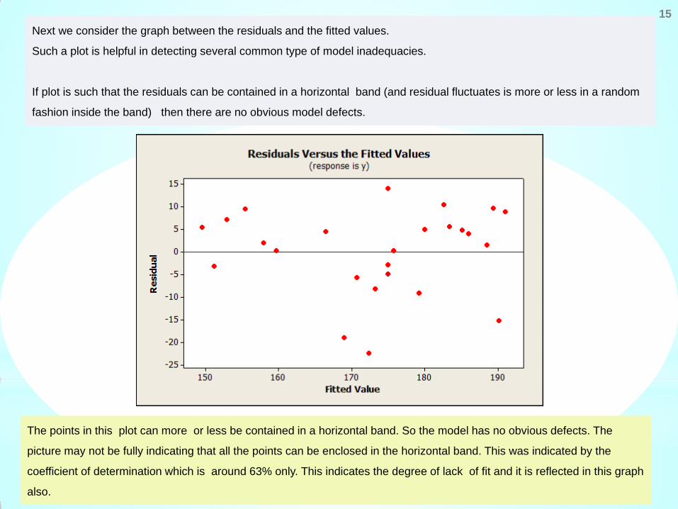
15 Next we consider the graph between the residuals and the fitted values.
Such a plot is helpful in detecting several common type of model inadequacies.
If plot is such that the residuals can be contained in a horizontal band (and residual fluctuates is more or less in a random
fashion inside the band) then there are no obvious model defects.
The points in this plot can more or less be contained in a horizontal band. So the model has no obvious defects. The
picture may not be fully indicating that all the points can be enclosed in the horizontal band. This was indicated by the
coefficient of determination which is around 63% only. This indicates the degree of lack of fit and it is reflected in this graph
also.
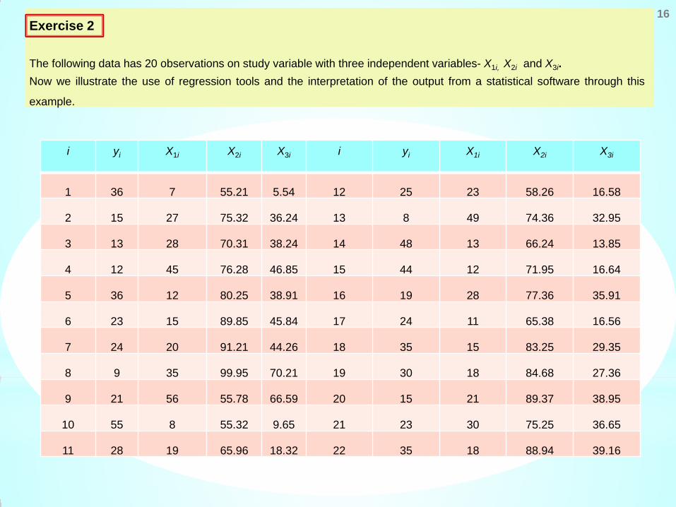
Exercise 2 The following data has 20 observations on study variable with three independent variables- X1i, X2i and X3i. Now we illustrate the use of regression tools and the interpretation of the output from a statistical software through this
example.
16
i yi X1i X2i X3i i yi X1i X2i X3i
1 36 7 55.21 5.54 12 25 23 58.26 16.58
2 15 27 75.32 36.24 13 8 49 74.36 32.95
3 13 28 70.31 38.24 14 48 13 66.24 13.85
4 12 45 76.28 46.85 15 44 12 71.95 16.64
5 36 12 80.25 38.91 16 19 28 77.36 35.91
6 23 15 89.85 45.84 17 24 11 65.38 16.56
7 24 20 91.21 44.26 18 35 15 83.25 29.35
8 9 35 99.95 70.21 19 30 18 84.68 27.36
9 21 56 55.78 66.59 20 15 21 89.37 38.95
10 55 8 55.32 9.65 21 23 30 75.25 36.65
11 28 19 65.96 18.32 22 35 18 88.94 39.16
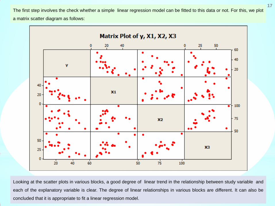
17 The first step involves the check whether a simple linear regression model can be fitted to this data or not. For this, we plot
a matrix scatter diagram as follows:
Looking at the scatter plots in various blocks, a good degree of linear trend in the relationship between study variable and
each of the explanatory variable is clear. The degree of linear relationships in various blocks are different. It can also be
concluded that it is appropriate to fit a linear regression model.
18
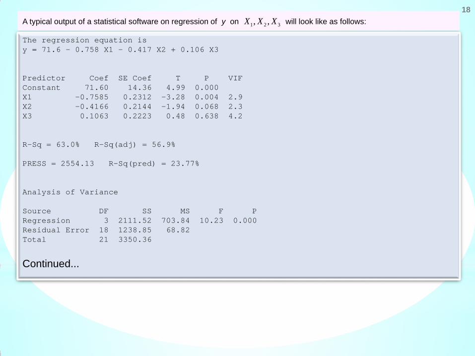
The regression equation is y = 71.6 - 0.758 X1 - 0.417 X2 + 0.106 X3 Predictor Coef SE Coef T P VIF Constant 71.60 14.36 4.99 0.000 X1 -0.7585 0.2312 -3.28 0.004 2.9 X2 -0.4166 0.2144 -1.94 0.068 2.3 X3 0.1063 0.2223 0.48 0.638 4.2 R-Sq = 63.0% R-Sq(adj) = 56.9% PRESS = 2554.13 R-Sq(pred) = 23.77% Analysis of Variance Source DF SS MS F P Regression 3 2111.52 703.84 10.23 0.000 Residual Error 18 1238.85 68.82 Total 21 3350.36
Continued...
A typical output of a statistical software on regression of y on will look like as follows: 1 2 3, ,X X X
19
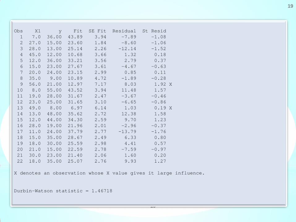
Obs X1 y Fit SE Fit Residual St Resid 1 7.0 36.00 43.89 3.94 -7.89 -1.08 2 27.0 15.00 23.60 1.84 -8.60 -1.06 3 28.0 13.00 25.14 2.26 -12.14 -1.52 4 45.0 12.00 10.68 3.66 1.32 0.18 5 12.0 36.00 33.21 3.56 2.79 0.37 6 15.0 23.00 27.67 3.61 -4.67 -0.63 7 20.0 24.00 23.15 2.99 0.85 0.11 8 35.0 9.00 10.89 4.72 -1.89 -0.28 9 56.0 21.00 12.97 7.17 8.03 1.92 X 10 8.0 55.00 43.52 3.94 11.48 1.57 11 19.0 28.00 31.67 2.47 -3.67 -0.46 12 23.0 25.00 31.65 3.10 -6.65 -0.86 13 49.0 8.00 6.97 6.14 1.03 0.19 X 14 13.0 48.00 35.62 2.72 12.38 1.58 15 12.0 44.00 34.30 2.59 9.70 1.23 16 28.0 19.00 21.96 2.01 -2.96 -0.37 17 11.0 24.00 37.79 2.77 -13.79 -1.76 18 15.0 35.00 28.67 2.49 6.33 0.80 19 18.0 30.00 25.59 2.98 4.41 0.57 20 21.0 15.00 22.59 2.78 -7.59 -0.97 21 30.0 23.00 21.40 2.06 1.60 0.20 22 18.0 35.00 25.07 2.76 9.93 1.27 X denotes an observation whose X value gives it large influence. Durbin-Watson statistic = 1.46718
19
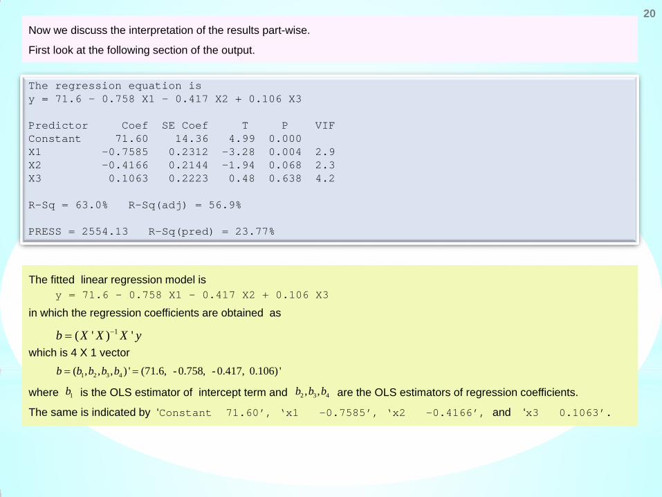
20 Now we discuss the interpretation of the results part-wise.
First look at the following section of the output.
The regression equation is y = 71.6 - 0.758 X1 - 0.417 X2 + 0.106 X3 Predictor Coef SE Coef T P VIF Constant 71.60 14.36 4.99 0.000 X1 -0.7585 0.2312 -3.28 0.004 2.9 X2 -0.4166 0.2144 -1.94 0.068 2.3 X3 0.1063 0.2223 0.48 0.638 4.2 R-Sq = 63.0% R-Sq(adj) = 56.9% PRESS = 2554.13 R-Sq(pred) = 23.77%
The fitted linear regression model is y = 71.6 - 0.758 X1 - 0.417 X2 + 0.106 X3
in which the regression coefficients are obtained as
which is 4 X 1 vector
where is the OLS estimator of intercept term and are the OLS estimators of regression coefficients.
The same is indicated by ‘Constant 71.60’, ‘x1 -0.7585’, ‘x2 -0.4166’, and ‘x3 0.1063’.
1( ' ) 'b X X X y−=
1 2 3 4( , , , ) ' (71.6, - 0.758, - 0.417, 0.106) 'b b b b b= =
1b 2 3 4, ,b b b
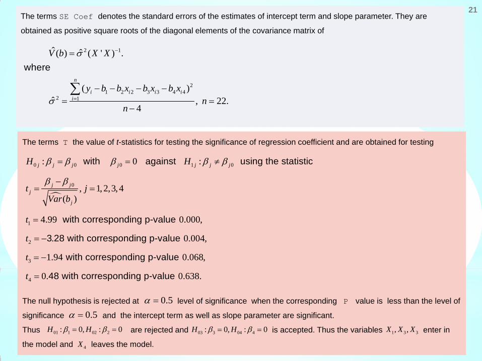
21 The terms SE Coef denotes the standard errors of the estimates of intercept term and slope parameter. They are
obtained as positive square roots of the diagonal elements of the covariance matrix of
2 1
21 2 2 3 3 4 4
2 1
ˆ ˆ( ) ( ' ) .
( )ˆ , 22.
4
where
n
i i i ii
V b X X
y b b x b x b xn
n
σ
σ
−
=
=
− − − −= =
−
∑
The terms T the value of t-statistics for testing the significance of regression coefficient and are obtained for testing
The null hypothesis is rejected at level of significance when the corresponding P value is less than the level of
significance and the intercept term as well as slope parameter are significant.
Thus are rejected and is accepted. Thus the variables enter in
the model and leaves the model.
0 0 0 1 0
0
1
2
3
: 0 :
, 1, 2,3, 4( )
4.99 0.000,
. 0.004,
1.94
with against using the statistic
with corresponding p-value
3 28 with corresponding p-value
with corresp
j j j j j j j
j jj
j
H H
t jVar b
t
t
t
β β β β β
β β
= = ≠
−= =
=
= −
= −
4
0.068,
0. 0.638.
onding p-value
48 with corresponding p-value t =
0.5α =
01 1 02 2: 0, : 0H Hβ β= = 03 3 04 4: 0, : 0H Hβ β= = 1 3 3, ,X X X
4X
0.5α =
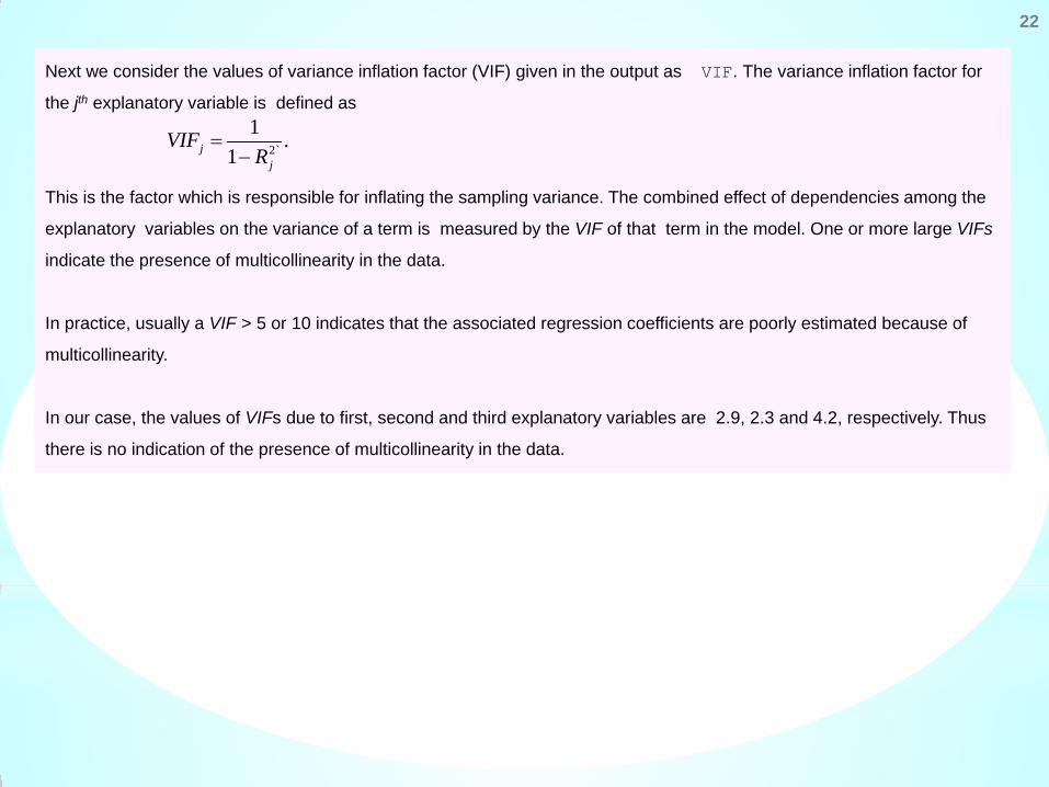
Next we consider the values of variance inflation factor (VIF) given in the output as VIF. The variance inflation factor for
the jth explanatory variable is defined as
This is the factor which is responsible for inflating the sampling variance. The combined effect of dependencies among the
explanatory variables on the variance of a term is measured by the VIF of that term in the model. One or more large VIFs
indicate the presence of multicollinearity in the data.
In practice, usually a VIF > 5 or 10 indicates that the associated regression coefficients are poorly estimated because of
multicollinearity.
In our case, the values of VIFs due to first, second and third explanatory variables are 2.9, 2.3 and 4.2, respectively. Thus
there is no indication of the presence of multicollinearity in the data.
2`
1 .1j
j
VIFR
=−
22
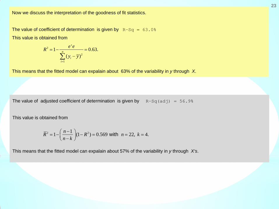
23 Now we discuss the interpretation of the goodness of fit statistics.
The value of coefficient of determination is given by R-Sq = 63.0%
This value is obtained from
This means that the fitted model can expalain about 63% of the variability in y through X.
2
2
1
'1 0.63.( )
n
ii
e eRy y
=
= − =−∑
The value of adjusted coefficient of determination is given by R-Sq(adj) = 56.9%
This value is obtained from
This means that the fitted model can expalain about 57% of the variability in y through X‘s.
2 211 (1 ) 0.569 22, 4. with nR R n kn k− = − − = = = −
24
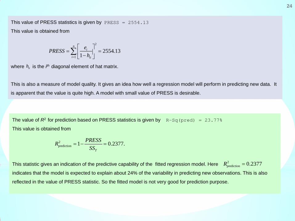
This value of PRESS statistics is given by PRESS = 2554.13
This value is obtained from
where is the ith diagonal element of hat matrix.
This is also a measure of model quality. It gives an idea how well a regression model will perform in predicting new data. It
is apparent that the value is quite high. A model with small value of PRESS is desirable.
2
12554.13
1
ni
i ii
ePRESSh=
= = − ∑
The value of R2 for prediction based on PRESS statistics is given by R-Sq(pred) = 23.77%
This value is obtained from
This statistic gives an indication of the predictive capability of the fitted regression model. Here
indicates that the model is expected to explain about 24% of the variability in predicting new observations. This is also
reflected in the value of PRESS statistic. So the fitted model is not very good for prediction purpose.
2prediction 1 0.2377.
T
PRESSRSS
= − =
2prediction 0.2377R =
iih
25
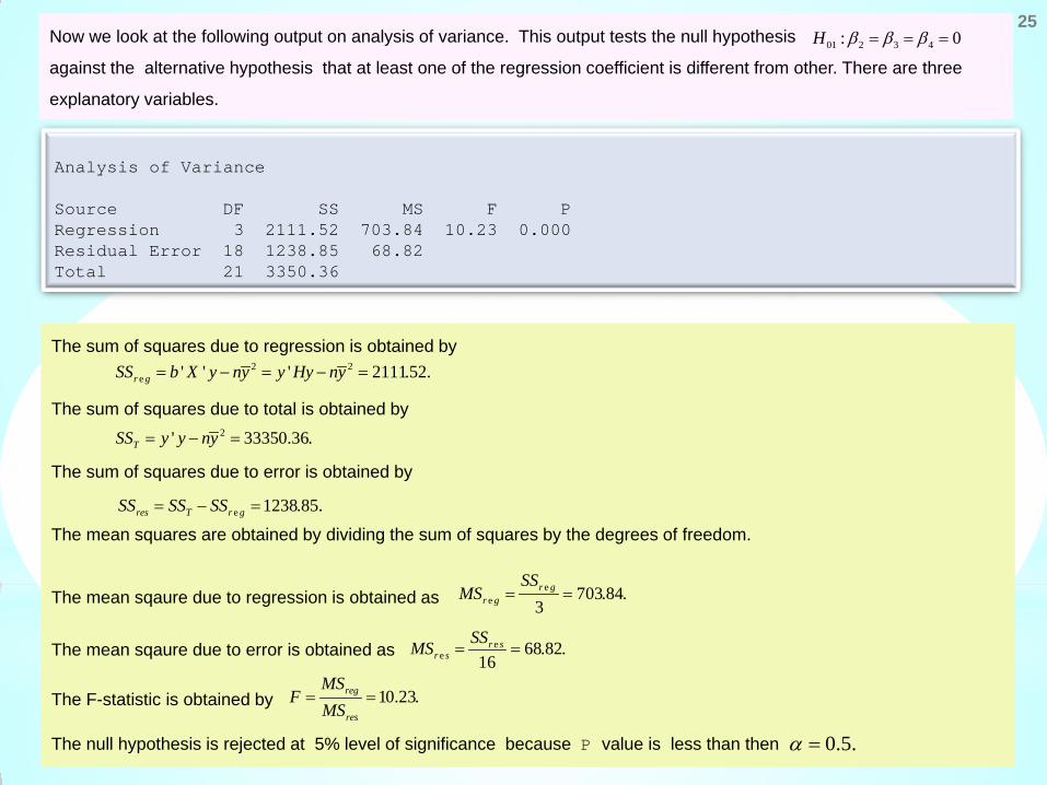
Analysis of Variance Source DF SS MS F P Regression 3 2111.52 703.84 10.23 0.000 Residual Error 18 1238.85 68.82 Total 21 3350.36
Now we look at the following output on analysis of variance. This output tests the null hypothesis
against the alternative hypothesis that at least one of the regression coefficient is different from other. There are three
explanatory variables.
01 2 3 4: 0H β β β= = =
The sum of squares due to regression is obtained by
The sum of squares due to total is obtained by
The sum of squares due to error is obtained by
The mean squares are obtained by dividing the sum of squares by the degrees of freedom.
The mean sqaure due to regression is obtained as
The mean sqaure due to error is obtained as
The F-statistic is obtained by
The null hypothesis is rejected at 5% level of significance because P value is less than then
2 2e ' ' ' 2111.52.r gSS b X y ny y Hy ny= − = − =
2' 33350.36.TSS y y ny= − =
e 1238.85.res T r gSS SS SS= − =
ee 703.84.
3r g
r g
SSMS = =
ee 68.82.
16r s
r sSSMS = =
10.23.reg
res
MSF
MS= =
0.5.α =
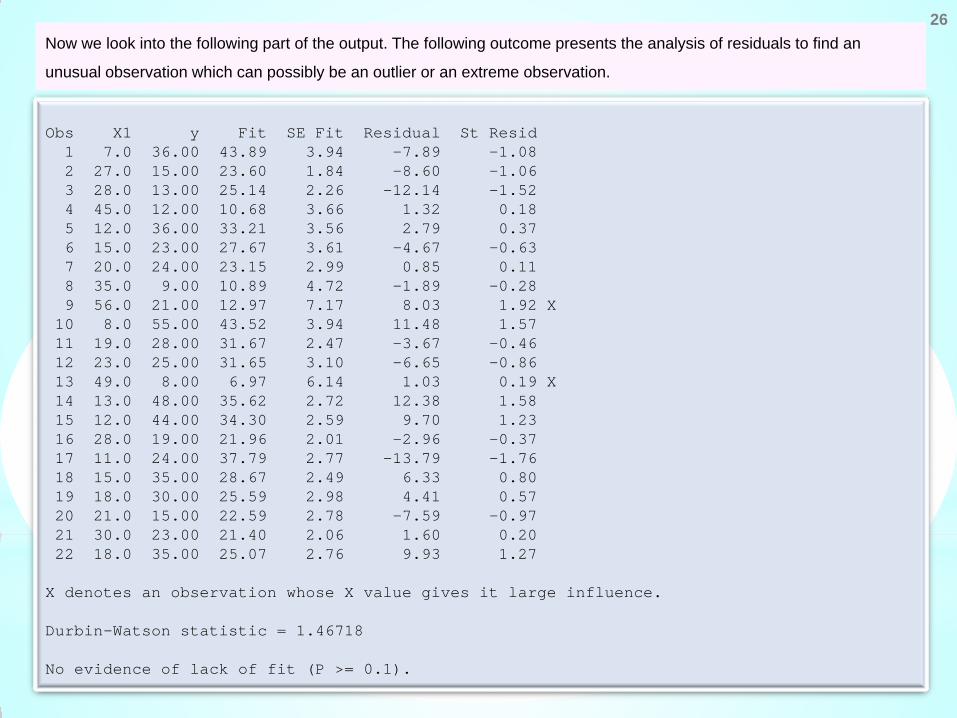
Obs X1 y Fit SE Fit Residual St Resid 1 7.0 36.00 43.89 3.94 -7.89 -1.08 2 27.0 15.00 23.60 1.84 -8.60 -1.06 3 28.0 13.00 25.14 2.26 -12.14 -1.52 4 45.0 12.00 10.68 3.66 1.32 0.18 5 12.0 36.00 33.21 3.56 2.79 0.37 6 15.0 23.00 27.67 3.61 -4.67 -0.63 7 20.0 24.00 23.15 2.99 0.85 0.11 8 35.0 9.00 10.89 4.72 -1.89 -0.28 9 56.0 21.00 12.97 7.17 8.03 1.92 X 10 8.0 55.00 43.52 3.94 11.48 1.57 11 19.0 28.00 31.67 2.47 -3.67 -0.46 12 23.0 25.00 31.65 3.10 -6.65 -0.86 13 49.0 8.00 6.97 6.14 1.03 0.19 X 14 13.0 48.00 35.62 2.72 12.38 1.58 15 12.0 44.00 34.30 2.59 9.70 1.23 16 28.0 19.00 21.96 2.01 -2.96 -0.37 17 11.0 24.00 37.79 2.77 -13.79 -1.76 18 15.0 35.00 28.67 2.49 6.33 0.80 19 18.0 30.00 25.59 2.98 4.41 0.57 20 21.0 15.00 22.59 2.78 -7.59 -0.97 21 30.0 23.00 21.40 2.06 1.60 0.20 22 18.0 35.00 25.07 2.76 9.93 1.27 X denotes an observation whose X value gives it large influence. Durbin-Watson statistic = 1.46718 No evidence of lack of fit (P >= 0.1).
Now we look into the following part of the output. The following outcome presents the analysis of residuals to find an
unusual observation which can possibly be an outlier or an extreme observation.
26
27
The Durbin Watson statistics is obtained from Durbin-Watson statistic = 1.46718
Its value is obtained from
At d = 2, it is indicated that there is no first order autocorrelation in the data. As the value d = 1.47 is less than 2, so it
indicates the possibility of presence of first order positive autocorrelation in the data.
( )21
2
2
1
1.46718.
n
t tt
n
tt
e ed
e
−=
=
−= =∑
∑
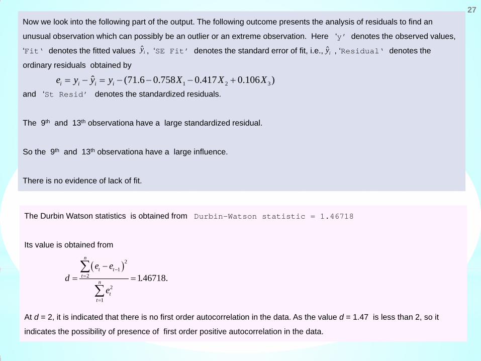
Now we look into the following part of the output. The following outcome presents the analysis of residuals to find an
unusual observation which can possibly be an outlier or an extreme observation. Here ‘y’ denotes the observed values,
‘Fit‘ denotes the fitted values , ‘SE Fit’ denotes the standard error of fit, i.e., , ‘Residual‘ denotes the
ordinary residuals obtained by
and ‘St Resid’ denotes the standardized residuals.
The 9th and 13th observationa have a large standardized residual.
So the 9th and 13th observationa have a large influence.
There is no evidence of lack of fit.
ˆiy
1 2 3ˆ (71.6 0.758 0.417 0.106 )i i i ie y y y X X X= − = − − − +
ˆiy
28
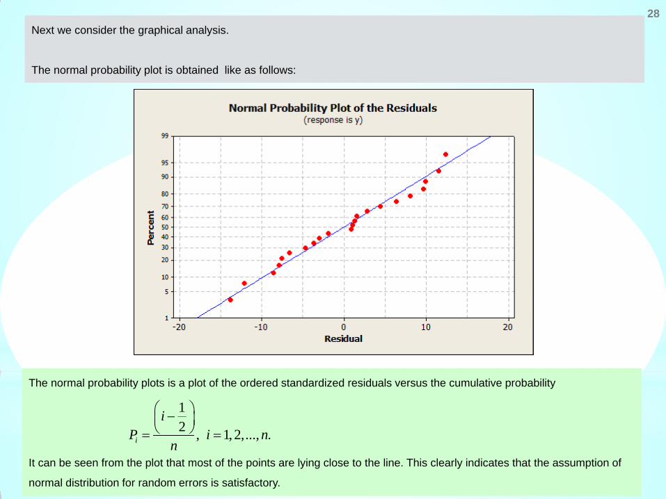
Next we consider the graphical analysis.
The normal probability plot is obtained like as follows:
The normal probability plots is a plot of the ordered standardized residuals versus the cumulative probability
It can be seen from the plot that most of the points are lying close to the line. This clearly indicates that the assumption of
normal distribution for random errors is satisfactory.
12 , 1,2,..., .i
iP i n
n
− = =
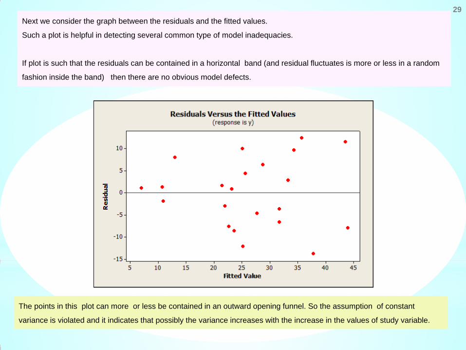
29 Next we consider the graph between the residuals and the fitted values.
Such a plot is helpful in detecting several common type of model inadequacies.
If plot is such that the residuals can be contained in a horizontal band (and residual fluctuates is more or less in a random
fashion inside the band) then there are no obvious model defects.
The points in this plot can more or less be contained in an outward opening funnel. So the assumption of constant
variance is violated and it indicates that possibly the variance increases with the increase in the values of study variable.