Embed Size (px)
Citation preview

Model Selection in a
Multi-Hypothesis Test Setting:
Applications in
Financial Econometrics
DCU Business School
December, 2017
Author:
Francesco P. Esposito
Supervisor:
Dr. Mark Cummins
Thesis submitted to Dublin City University Business
School in partial fulfilment of the requirements for the
Degree of Doctor of Philosophy


I hereby certify that this material, which I now submit for assessment on the programme of study
leading to the award of Ph.D. is entirely my own work, and that I have exercised reasonable care
to ensure that the work is original, and does not to the best of my knowledge breach any law of
copyright, and has not been taken from the work of others save and to the extent that such work
has been cited and acknowledged within the text of my work.
Signed ID No.: 12211600 Date:


Acknowledgments
I would like to express my sincere gratitude to my advisor Dr. Mark Cummins for his wise suggestions
and guidance and, furthermore, for having allowed the realisation of this project under unconventional
circumstances.
Besides Mark, I would like to thank Ludovica, for her precious friendship through the years and her
encouraging words.
Foremost, I wish to thank my wife Tina for her love, trust and patience.


Model Selection in a Multi-Hypothesis Test Setting:Applications in Financial Econometrics
F. P. Esposito
Abstract
In this thesis, we investigate model selection in a general setting and performseveral exercises in financial econometrics. We present the multi-hypothesistesting (MHT) framework, with which we design different type of model com-parisons. We distinguish between test of model performance significance, ofrelative and absolute model performance and apply our framework to mar-ket risk forecasting model, to latent factor jump-diffusion models employed forthe estimation of the statistical measure of an equity index, as well as to eq-uity option pricing models. We develop original tests and, with regard to theproper exercise of model selection from an initial battery of models withoutany reference to a benchmark model, we combine the MHT approach with themodel confidence set (MCS) to deliver a novel test of model comparison thatis performed along with the established version of the MCS, as well as with analternative simplified new MCS test that are detailed in the course of this work.We collect empirical evidence concerning model comparison in several subjects.With respect to market risk forecasting models, we have found that models cap-turing volatility clustering or targeting directly an auto-correlated conditionaldistribution percentile, perform better than the target model set and in partic-ular, better than the historical simulation, widely employed by practitioners,and better than the so called RiskMetrics model. With respect to the equityindex data dynamics, we have found that the popular affine jump-diffusionmodel requires a CEV augmentation to perform appropriately and that thosemodels are slightly overperformed by an alternative stochastic volatility model,characterised by stochastic hazard with high frequency small jumps. The testperformed over a large model set employed in the option pricing exercise pointsto a wide similarity of the results obtained by the many model specificationsof the superior exponential volatility model, therefore suggesting a more care-ful adjustment of the model complexity. The model selection framework hasproven very flexible in dealing with the varied collection of statistical problems.In particular, our main contribution represented by the generalised MHT basedMCS test provides a method for model selection that is robust to finite sampledistribution and that has the advantage of an adjustable tolerance for falserejections, allowing conservative to aggressive testing profiles.
Keywords: Multi-hypothesis test, generalised family-wise error rate, tail probability of false discovery proportion, station-ary bootstrap, step-down algorithm, model confidence set, value-at-risk, expected shortfall, likelihood function, second ordernon-linear filter, jump-diffusion, stochastic volatility, stochastic hazard, option pricing model, partial integral-differentialequation, finite difference method.


Contents
1 Model Selection Framework 1
1.1 The Model Selection Strategy . . . . . . . . . . . . . . . . . . . . . . . . . . . . . . . . . . 4
1.2 Multiple Hypothesis Testing . . . . . . . . . . . . . . . . . . . . . . . . . . . . . . . . . . . 5
1.2.1 The Implementation of the MHT Procedure . . . . . . . . . . . . . . . . . . . . . . 8
1.2.2 The Step-Down Algorithm . . . . . . . . . . . . . . . . . . . . . . . . . . . . . . . . 10
1.2.3 The Stationary Bootstrap . . . . . . . . . . . . . . . . . . . . . . . . . . . . . . . . 12
1.3 The Model Confidence Set . . . . . . . . . . . . . . . . . . . . . . . . . . . . . . . . . . . . 14
1.3.1 The max -MCS . . . . . . . . . . . . . . . . . . . . . . . . . . . . . . . . . . . . . . 15
1.3.2 The t-MCS . . . . . . . . . . . . . . . . . . . . . . . . . . . . . . . . . . . . . . . . 17
1.3.3 The γ-MCS . . . . . . . . . . . . . . . . . . . . . . . . . . . . . . . . . . . . . . . . 19
1.4 Thesis Summary . . . . . . . . . . . . . . . . . . . . . . . . . . . . . . . . . . . . . . . . . 21
1.5 Concluding Remarks . . . . . . . . . . . . . . . . . . . . . . . . . . . . . . . . . . . . . . . 26
2 Model Selection of Market Risk Models 27
2.1 The Conditional Distribution Model Set . . . . . . . . . . . . . . . . . . . . . . . . . . . . 29
2.2 Model Comparison Testing . . . . . . . . . . . . . . . . . . . . . . . . . . . . . . . . . . . 32
2.3 Experimental Section . . . . . . . . . . . . . . . . . . . . . . . . . . . . . . . . . . . . . . . 34
2.3.1 Preliminary Considerations . . . . . . . . . . . . . . . . . . . . . . . . . . . . . . . 34

CONTENTS
2.3.2 Market Data Experiment . . . . . . . . . . . . . . . . . . . . . . . . . . . . . . . . 37
2.4 Concluding Remarks . . . . . . . . . . . . . . . . . . . . . . . . . . . . . . . . . . . . . . . 40
Tables . . . . . . . . . . . . . . . . . . . . . . . . . . . . . . . . . . . . . . . . . . . . . . . . . . 42
3 Model Selection of Jump-Diffusion Models 55
3.0.1 Some clarifications . . . . . . . . . . . . . . . . . . . . . . . . . . . . . . . . . . . . 58
3.1 The Jump-Diffusion Model Set . . . . . . . . . . . . . . . . . . . . . . . . . . . . . . . . . 61
3.1.1 Parameter Estimation . . . . . . . . . . . . . . . . . . . . . . . . . . . . . . . . . . 64
3.1.2 The Second Order Non-Linear Filter . . . . . . . . . . . . . . . . . . . . . . . . . . 65
3.2 Model Comparison Testing . . . . . . . . . . . . . . . . . . . . . . . . . . . . . . . . . . . 66
3.2.1 Likelihood Ratio . . . . . . . . . . . . . . . . . . . . . . . . . . . . . . . . . . . . . 67
3.2.2 Distance from the Latent Component . . . . . . . . . . . . . . . . . . . . . . . . . 68
3.2.3 LR with Latent Component . . . . . . . . . . . . . . . . . . . . . . . . . . . . . . . 69
3.3 Experimental Section . . . . . . . . . . . . . . . . . . . . . . . . . . . . . . . . . . . . . . . 70
3.3.1 Preliminary Considerations . . . . . . . . . . . . . . . . . . . . . . . . . . . . . . . 70
3.3.1.1 Benchmarking the NLF2 with Particle Filtering . . . . . . . . . . . . . . 74
3.3.2 Monte Carlo Experiment . . . . . . . . . . . . . . . . . . . . . . . . . . . . . . . . 76
3.3.3 Market Data Experiment . . . . . . . . . . . . . . . . . . . . . . . . . . . . . . . . 79
3.4 Concluding Remarks . . . . . . . . . . . . . . . . . . . . . . . . . . . . . . . . . . . . . . . 82
Tables . . . . . . . . . . . . . . . . . . . . . . . . . . . . . . . . . . . . . . . . . . . . . . . . . . 84
Figures . . . . . . . . . . . . . . . . . . . . . . . . . . . . . . . . . . . . . . . . . . . . . . . . . 101
4 Model Selection of Derivative Pricing JD Models 107
4.1 The Derivative Pricing Model Set . . . . . . . . . . . . . . . . . . . . . . . . . . . . . . . . 109
4.2 Model Comparison Testing . . . . . . . . . . . . . . . . . . . . . . . . . . . . . . . . . . . 112
4.2.1 Mispricing MSE . . . . . . . . . . . . . . . . . . . . . . . . . . . . . . . . . . . . . 113
4.3 Experimental Section . . . . . . . . . . . . . . . . . . . . . . . . . . . . . . . . . . . . . . . 115
4.3.1 Preliminary Considerations . . . . . . . . . . . . . . . . . . . . . . . . . . . . . . . 115
4.3.2 Market Data Experiment . . . . . . . . . . . . . . . . . . . . . . . . . . . . . . . . 119
4.4 Concluding Remarks . . . . . . . . . . . . . . . . . . . . . . . . . . . . . . . . . . . . . . . 121
Tables . . . . . . . . . . . . . . . . . . . . . . . . . . . . . . . . . . . . . . . . . . . . . . . . . . 123
Figures . . . . . . . . . . . . . . . . . . . . . . . . . . . . . . . . . . . . . . . . . . . . . . . . . 131
5 Conclusions 137
Bibliography 143
A Algorithms 153
A.1 The Approximate Likelihood Function . . . . . . . . . . . . . . . . . . . . . . . . . . . . . 153
A.1.1 The Marginalisation Procedure . . . . . . . . . . . . . . . . . . . . . . . . . . . . . 154
A.1.2 The Approximation of the Transition Density . . . . . . . . . . . . . . . . . . . . . 155
A.2 The PIDE solution . . . . . . . . . . . . . . . . . . . . . . . . . . . . . . . . . . . . . . . . 156
A.3 The Nonlinear Filter . . . . . . . . . . . . . . . . . . . . . . . . . . . . . . . . . . . . . . . 158

CONTENTS
A.3.1 The Time-Propagation Equation . . . . . . . . . . . . . . . . . . . . . . . . . . . . 160
A.3.2 The Update Equation . . . . . . . . . . . . . . . . . . . . . . . . . . . . . . . . . . 163
A.3.3 The Expectation Proxy . . . . . . . . . . . . . . . . . . . . . . . . . . . . . . . . . 164
A.3.4 The NLF2 of the SD and SH Classes . . . . . . . . . . . . . . . . . . . . . . . . . . 166
A.4 Model Transformations . . . . . . . . . . . . . . . . . . . . . . . . . . . . . . . . . . . . . . 167
B Pseudo-Codes 171
B.1 The AML algorithm . . . . . . . . . . . . . . . . . . . . . . . . . . . . . . . . . . . . . . . 172
B.2 The SIR−PF algorithm . . . . . . . . . . . . . . . . . . . . . . . . . . . . . . . . . . . . . 174
B.3 The MSE algorithm . . . . . . . . . . . . . . . . . . . . . . . . . . . . . . . . . . . . . . . 175


List of Tables
1 VaR and ExS Forecasting Models . . . . . . . . . . . . . . . . . . . . . . . . . . . . . . . . 42
2 VaR MHT . . . . . . . . . . . . . . . . . . . . . . . . . . . . . . . . . . . . . . . . . . . . . 43
3 ExS MHT . . . . . . . . . . . . . . . . . . . . . . . . . . . . . . . . . . . . . . . . . . . . . 44
4 L/V VaR MHT . . . . . . . . . . . . . . . . . . . . . . . . . . . . . . . . . . . . . . . . . . 45
5 H/V VaR MHT . . . . . . . . . . . . . . . . . . . . . . . . . . . . . . . . . . . . . . . . . . 46
6 MCS VaR 1% 1d . . . . . . . . . . . . . . . . . . . . . . . . . . . . . . . . . . . . . . . . . 47
7 MCS VaR 5% 1d . . . . . . . . . . . . . . . . . . . . . . . . . . . . . . . . . . . . . . . . . 48
8 MCS ExS 1% 1d . . . . . . . . . . . . . . . . . . . . . . . . . . . . . . . . . . . . . . . . . 49
9 MCS ExS 5% 1d . . . . . . . . . . . . . . . . . . . . . . . . . . . . . . . . . . . . . . . . . 50
10 MCS VaR 1% 2w . . . . . . . . . . . . . . . . . . . . . . . . . . . . . . . . . . . . . . . . . 51
11 MCS VaR 5% 2w . . . . . . . . . . . . . . . . . . . . . . . . . . . . . . . . . . . . . . . . . 52
12 MCS ExS 1% 2w . . . . . . . . . . . . . . . . . . . . . . . . . . . . . . . . . . . . . . . . . 53
13 MCS ExS 5% 2w . . . . . . . . . . . . . . . . . . . . . . . . . . . . . . . . . . . . . . . . . 54
14 Model Set Acronyms . . . . . . . . . . . . . . . . . . . . . . . . . . . . . . . . . . . . . . . 84
15 Standard Models and the Model Set . . . . . . . . . . . . . . . . . . . . . . . . . . . . . . 85
16 Simulation MHT Model Parameters and Standardised Moments . . . . . . . . . . . . . . . 86
17 Financial Market Data Model Parameters Estimates . . . . . . . . . . . . . . . . . . . . . 87

LIST OF TABLES
18 Simulated LRMHT . . . . . . . . . . . . . . . . . . . . . . . . . . . . . . . . . . . . . . . . 88
19 Simulated LCMHT. . . . . . . . . . . . . . . . . . . . . . . . . . . . . . . . . . . . . . . . 89
20 Simulated LRMCS-max. . . . . . . . . . . . . . . . . . . . . . . . . . . . . . . . . . . . . . 90
21 Simulated LRMCS-γ. . . . . . . . . . . . . . . . . . . . . . . . . . . . . . . . . . . . . . . 91
22 Simulated LRMCS-t. . . . . . . . . . . . . . . . . . . . . . . . . . . . . . . . . . . . . . . . 92
23 Simulated LCMCS-max. . . . . . . . . . . . . . . . . . . . . . . . . . . . . . . . . . . . . . 93
24 Simulated LCMCS-γ. . . . . . . . . . . . . . . . . . . . . . . . . . . . . . . . . . . . . . . . 94
25 Simulated LCMCS-t. . . . . . . . . . . . . . . . . . . . . . . . . . . . . . . . . . . . . . . . 95
26 Market Data LRMHT. . . . . . . . . . . . . . . . . . . . . . . . . . . . . . . . . . . . . . . 96
27 Market Data TGMHT. . . . . . . . . . . . . . . . . . . . . . . . . . . . . . . . . . . . . . . 97
28 Market Data LRLCMHT. . . . . . . . . . . . . . . . . . . . . . . . . . . . . . . . . . . . . 98
29 Market Data MCS. . . . . . . . . . . . . . . . . . . . . . . . . . . . . . . . . . . . . . . . . 99
30 The NLF2 and the SIR Particle Filter. . . . . . . . . . . . . . . . . . . . . . . . . . . . . . 100
31 The Call Option Average Implied Volatility. . . . . . . . . . . . . . . . . . . . . . . . . . . 123
32 The Put Option Average Implied Volatility. . . . . . . . . . . . . . . . . . . . . . . . . . . 124
33 The Call Option Data Distribution. . . . . . . . . . . . . . . . . . . . . . . . . . . . . . . 125
34 The Put Option Data Distribution. . . . . . . . . . . . . . . . . . . . . . . . . . . . . . . . 126
35 The OTM Call/Put Option Average Implied Volatility. . . . . . . . . . . . . . . . . . . . . 127
36 The OTM Call/Put Option Data Distribution. . . . . . . . . . . . . . . . . . . . . . . . . 128
37 Bootstrap MCS-γ fix at 20% and 40% OTM and ALL sample. . . . . . . . . . . . . . . . 129
38 Bootstrap MCS-max at 10% ALL sample. . . . . . . . . . . . . . . . . . . . . . . . . . . . 130

List of Figures
1 The Likelihood Function Algorithm. . . . . . . . . . . . . . . . . . . . . . . . . . . . . . . 101
2 An example of Information Loss. . . . . . . . . . . . . . . . . . . . . . . . . . . . . . . . . 102
3 The Distributional Shape of the Model Set. . . . . . . . . . . . . . . . . . . . . . . . . . . 103
4 Several Implementation Issues. . . . . . . . . . . . . . . . . . . . . . . . . . . . . . . . . . 104
5 Market Data Applications. . . . . . . . . . . . . . . . . . . . . . . . . . . . . . . . . . . . . 105
6 S&P500 Index Level. . . . . . . . . . . . . . . . . . . . . . . . . . . . . . . . . . . . . . . . 131
7 Put/Call Parity Distribution. . . . . . . . . . . . . . . . . . . . . . . . . . . . . . . . . . . 132
8 The Selection of the Option Price Sample. . . . . . . . . . . . . . . . . . . . . . . . . . . . 133
9 Time Series Features of the Option Price Sample. . . . . . . . . . . . . . . . . . . . . . . . 134
10 The RMSE Time Series. . . . . . . . . . . . . . . . . . . . . . . . . . . . . . . . . . . . . . 135
11 The Volatility Surface Quantile Regression. . . . . . . . . . . . . . . . . . . . . . . . . . . 136

1 CHAPTER 1. MODEL SELECTION FRAMEWORK
Model Selection Framework
The question that is debated in this thesis is central to a wide range of statistical applications. The
research objective can be summarised as follows: given a set of models returning output that is data
explanatory or data forecasting, which model or which model subset produces the best performance?
Further characterisation is required by demanding: what degree of uncertainty can be associated with,
and how robust is the decision concerning the best model set? This task is referred to as model selection.
In statistics, this term is usually associated with the comparison of models as partial representations of
the data generating process (DGP). In this work, on the contrary, we use this label in a wider sense. In
general terms, we deal with a given set of objects, namely models, which characterise the execution of
a certain action on the experimental observations or indirect measurements of the phenomenon under
analysis, that is the data. The concept of a “model” has to be interpreted in abstract terms as a set of
rules prescribing the data processing function, although it will ultimately be associated with a probability
distribution hypothesis1. The action of the model is intended as a transformation of the experimental
1 The term model that is adopted throughout this thesis is in line with the practiotioners’ use of this word. In Office ofthe Comptroller of the Currency (2011) “the term model refers to a quantitative method, system, or approach that appliesstatistical, economic, financial or mathematical theories, techniques, and assumptions to process input data into quantitativeestimates. A model consists of three components: an information component, which delivers assumptions and data to themodel; a processing component, which transforms inputs into estimates; a reporting component, which translates thoseestimates into useful business information.” Nonetheless, with very few exceptions in this manuscript, a model might still

2
data that provides explanatory information about or forecasts the behaviour of the underlying system of
variables. The result of this action feeds a model performance indicator, which enables the comparison of
the model set, as prescribed by the model selection criterion. The focus is tilted towards the statistical
distribution of this loss function rather than to the approximation of the DGP, two aspects of the decision
problem that might not directly coincide as such, for instance, in the linear constrained regression prob-
lem of Toro-Vizcarrondo and Wallace (1968), whereby the minimum squared error criterion is regarded
as the discerning factor for the evaluation of the model performance, whereas testing the likelihood of
the model restrictions does not necessarily provide a matching result. In the lecture note Rao and Wu
(2001), the authors propose a classification of the model selection process, which is mostly methodologi-
cal. According to the authors, model selection can be characterised into several problem types. In fact,
it is either conducted as a sequence of hypotheses testing, as a forecasting error minimisation problem,
through information theoretic criteria, based on bootstrap methods or approached in a Bayesian set-up.
Other categories that are mentioned in the lecture note pertain to specific statistical problem classes, such
as cross-validation, order selection in time series, categorical data analysis, non-parametric regression and
data-oriented penalty. The literature on the subject is overwhelming, therefore this introduction does
not serve as a complete review of such a vast and varied subject matter. In this section, we demarcate
this research and identify the areas from which we draw the methodology and the instruments to devise
the econometric applications presented in this thesis.
Model selection is deeply rooted in the origins of statistics. The major problem is that of model specifi-
cation, which can be traced back to discipline establishing works such as Fisher (1922, 1924) and Pearson
(1936), which advocated, respectively, the method of maximum likelihood and the method of moments
as procedures for model identification. Tests for model specification were devised later involving a single
specification hypothesis on the model significance, such as the Lagrange multiplier test (Silvey, 1959;
Breusch and Pagan, 1980), the Hausman (1978) test, the information matrix test and the score test of
White (1982), the Newey (1985) test, the approach of Wooldridge (1990). Tests involving direct pairwise
model comparisons can be referenced, for instance, to the Wald (1943) test for model parameters restric-
tions, the likelihood ratio statistic of Wilks (1938) and more generally the testing framework of Vuong
(1989). Eventually, it was the work of Akaike (1974, 1981) that provided the model specification task with
a criterion allowing for a more extensive model comparison. Furthermore in the context of model specifi-
cation, a direct pairwise comparison exploiting the AIC was pursued with the test of Linhart (1988), which
was later employed in conjunction with the model subset selection procedure of Gupta and Huang (1976)
to construct the confidence set of models of Shimodaira (1998), probably the first procedure providing a
multiple comparison model selection test with a general application in the realm of maximum likelihood.
In this perspective, this aspect of model selection as a multiple comparison statistical test is central to
this thesis work. We adopt the multiple hypothesis testing (MHT) framework of Beran (1988a,b, 1990,
2003) and Romano and Wolf (2005a, 2007, 2010) in constructing balanced confidence set based multiple
comparison tests for the sake of model selection. For our purposes, we seek a general procedure that is
not only applicable to likelihood tests but that is capable of handling virtually any kind of model com-
parison problem, requiring a minimum set of assumptions. The general setup is related to several works
be associated with an hypothesis regarding the DGP, although we employ the former definition.

3 CHAPTER 1. MODEL SELECTION FRAMEWORK
in model forecasting performance, such as Diebold and Mariano (1995), West (1996) in a pairwise model
comparison setting, and the works of White (2000) and Hansen (2005), in a multiple comparison context.
Although not only confined to forecasting model comparison, the latter multiple comparison tests suffer
from the lack of ability to identify the best performing models, yielding an inference as to whether the
model set contains items that perform better than a given reference model. This fact has been noted in
Romano and Wolf (2005b), who deliver a step-wise procedure version of the reality check approach of
White (2000) and Hansen (2005) that isolates the subset of models that perform better than the reference
model, see also Romano et al. (2008). We indicate this type of test as relative model comparison. Finally,
we remark that, whenever the problem is configured such that the specification of a reference model is
not required, the collection of multiple model comparison tests just referenced are limited. We indicate
the problem of model selection without a pre-specified term of comparison as absolute model comparison.
In this regard, we build upon the Hansen et al. (2011) version of the model confidence set (MCS) to
design a generalised multiple hypothesis test for model comparison that does not require the choice of a
reference model, with several applications in financial econometrics showcased. This multiple comparison
model selection procedure, which we coin the γ-MCS, is a characterisation of the MHT controlling for
the number k of tolerated false discoveries and, in an extended version, the γ tail probability of the false
discovery proportion can also be triggered; both cases allow for a complete analysis of the set of model
comparisons. The hypotheses testing is structured to embed the complete multi-dimensional nature of
the model selection exercise and draw inference with respect to individual model comparisons, at the
same time controlling for test dependencies. The model selection procedures are powered by a simulation
engine represented by a type of block bootstrap device such as the stationary bootstrap of Politis and
Romano (1994a,b), rendering the test robust to finite sample statistic distribution. The bootstrap ap-
proach enables the method to handle virtually any model selection problem, without resorting to pivotal
results, in this case meaning without resorting to the asymptotic normality of the statistics. Thus, the
exercise is reduced to a matter of experimental design, an attractive characteristic for financial practi-
tioners. In fact, with the empirical applications in this thesis, we are able to construct model selection
procedures whereby the models are misspecified in nature and the model battery may contain parametric
and non parametric models, whereby we could could compare continuous and discrete time models, we
could include nested and non-nested model specifications, or further we could operate in a context of
partial information. In several applications, the exercise is worsened by the finite precision of the several
numerical procedures involved in the calculation of the crucial measures of model performance, a feature
that can be improved at the cost of overall computational demand.
With this Chapter 1, we provide the fundamental link between all parts of this thesis by means of formally
introducing the model selection approach pursued throughout. We introduce the general problem of test
dependencies, articulated and solved within the framework of Beran (1988a,b, 1990, 2003) and Romano
and Wolf (2005a, 2007, 2010), whereby the balanced confidence set for the MHT are constructed and
combined with generalised error controlling algorithms. Building on the model comparison test design
based on the loss function of Diebold and Mariano (1995), West (1996) White (2000) and Hansen (2005),
we outline performance significance and relative model comparison MHT. Finally, invoking the MCS
concept drawn by Hansen et al. (2011), we provide an original contribution to the literature by merging

1.1. THE MODEL SELECTION STRATEGY 4
the generalised MHT and the MCS to develop the γ-MCS test. In our interpretation, the MCS is a set re-
striction hinging on a preference relationship amongst the model set, which is ultimately defined through
a statistical test. The inference process delivers the equivalence set of best performing models that, al-
though preserves some coherence across different types of test, is not necessarily unique. We provide this
important insight through the construction of a simplified MCS test of model selection, which utilises
the same comparison strategy as the γ-MCS, but which does not retain its superior MHT properties.
We indicate this test as the t-MCS. In general, when the main model clusters are very distinct, the tests
tend to deliver the same results, whereas when the models are tightly competing, the test dependencies
play a major role, whereby the γ-MCS reveals greater flexibility in its model discrimination capability,
represented by the generalised controlling mechanism.
In the following Section 1.1 we develop the model selection strategy, whereas in Section 1.2 we present the
technical details for the construction of the multiple hypothesis test with balanced confidence intervals,
which represent the main instrument for the pursuing of the several model comparison exercises. In
Section 1.3 we characterise the procedure for discarding the benchmark model in the model selection test
and constructing the model confidence set. In this section, the main MCS test of Hansen et al. (2011) is
detailed, while the additional t-MCS and γ-MCS tests are presented. Section 1.4 provides an overview of
the thesis by introducing the motivation for and the layout of the chapter experiments, emphasising the
contributions and main findings in each case. Section 1.5 concludes this methodological chapter.
1.1 The Model Selection Strategy
In our set-up, a model is ultimately conceived as a conjecture on a probability distribution P, by which we
identify the model itself. We define the initial model set asM0 ≡ P0,P1, . . . ,Pm0. The performance
of model Pi ∈ M0 is measured by the data transform Li,t := L(Xt,Pi), that is a numerical function
of the data set Xt observed at time t, evaluated according to the model prescriptions defined by Pi. A
classic exercise of hypotheses testing that will be accomplished within the experimental part of Chapter 2
concerns the construction of tests of significance of the model performance, where the model performance
metric is compared with a target value, whenever this one can be defined. However, tests of this type are
not suited for the purpose of model comparison, as they do not involve pitting the models against one
another. In fact, models producing significant performances do not necessarily produce superior output
when contrasted with competitors. This brings us to the following discussion of methods for model com-
parison.
A model comparison is defined as the contrasting of models Pi and Pj , whose outcome is a preference
ordering that decides which model is best, or that both models are equivalent. Whenever model i is
preferred to model j, we write Pi Pj or Pj ≺ Pi and we say, respectively, that model i is superior
to model j or that model j is inferior to model i. The equivalence between the two models is written
as Pi ∼ Pj . The objective of this thesis is the characterisation of the decision rule establishing the
preference structure upon the model set M0. This task in general corresponds to a statistical testing
procedure that might involve a sequence of tests or a joint multivariate test, delivering in addition a

5 CHAPTER 1. MODEL SELECTION FRAMEWORK
model ranking system. In the model comparison framework we are devising, the model performance
measure L is a model loss function, that the lower this figure, the better. The reference metric is the
relative performance measure dij,t := Li,t−Lj,t, where the ordering is important. The testing procedures
presented in the rest of this chapter target either the quantity µij := E [dij,t], such that Pi Pj , if
µij < 0 or Pi ∼ Pj , if µij = 0. Whenever a model P0 ∈ M0 is attributed with the special role of being
a benchmark, we refer to this as a relative model performance test, where the objective is to determine
whetherM0 contains a model preferable to the benchmark. In the literature there are several examples
of relative performance tests such as the reality check (RC) of White (2000) or the superior predictive
ability (SPA) test of Hansen (2005). These types of tests are known to be very conservative2. In Chap-
ter 3 we present two applications of our alternative form of relative model performance test, whereby the
benchmark is either clearly identified, or the test is run by recursively selecting the benchmark model,
revealing model clusters and the full collection of model preferences. This feature might be useful in
suboptimal decision making, that is whenever the usage of the best model is prevented, the mapping of
the full set of model comparison results allows the choice of second best models. However, synthesising
the information provided by this form of test is subjective to some extent as it lacks a procedure for
the automatic selection of superior models. There, to address this, a contribution of this study is the
construction of a general model selection procedure in an MHT setting, designed to automatically select
the superior models from a given model set. We indicate this type of statistical test as an absolute model
performance test.
In the next section we introduce the generalised MHT procedure by which we construct the test of
significance of model performance, the relative performance test, as well as the main step of the MHT
based absolute model performance tests. In Section 1.3 we introduce the fundamental concept of MCS as
in Hansen et al. (2011), by which we complete the design of the novel γ-MCS along with the introduction
of more MCS tests.
1.2 Multiple Hypothesis Testing
A multiple hypothesis test is a statistical test on the set of hypotheses H1, . . . ,Hm. The distinctive
feature of the test is that the Hj ’s are considered jointly and hence the test statistic is, in general, an m
dimensional vector. The construction of a procedure for MHT requires some subtleties. When dealing
with multiple hypothesis testing the notions of a rejection region and confidence level acquire higher
complexity, and it is not immediate the translation of a single testing procedure into an MHT which
takes into account the multiple dimension of the decision under analysis. In the case of a single null H0
versus an alternative HA, the criterion in hypothesis testing prescribes the construction of a rejection2 The formal null hypothesis is H0 : maxi=1,...,m µ0i ≤ 0 which corresponds to the hypothesis that “no model in the
model set M0 is superior to the benchmark P0”. As noted in Corradi and Distaso (2011), the introduction of a poorlyperforming model, although it does not have any impact on the asymptotic value of the statistic because max1,...,m+1 µ0i =max1,...,m µ0i, it will certainly affect the percentiles and then the p-value of the statistic distribution. Indeed, the poorlyperforming model Pm+1 will have a consistent impact on the distribution of the max statistic. The introduction of apoorly performance model will therefore have the effect of inflating the p-value, which can actually be made large at will,by including bad performing objects in the target model set. This is a substantial limitation of the reality check, which stillpersists in the standardised version of the test, see Hansen (2005). To attenuate the dependence on the outlier bad model,the author proposes to discard the bootstrap generated performance measures that exceed an asymptotic threshold. It isnot clear, however, if the superior predictive ability test is more powerful than the reality check, cfr. Corradi and Distaso(2011).

1.2. MULTIPLE HYPOTHESIS TESTING 6
region Γ, whereby the inclusion of the sample determined statistic T ∈ Γ leads to the rejection of the
null hypothesis, whereas T /∈ Γ leads to its acceptance. The probability measure of the rejection region
P(Γ) = α represents the confidence level, which is the probability of committing a type I error that is
the rejection of H0 when it is true. A type II error occurs when T /∈ Γ implies the acceptance of the
null, while HA is actually true. The power of the test is given by 1 − P T /∈ Γ, s.t.|HA| = 1, where
in general terms |A| is the Boolean value of the event A. On the other hand, when considering the
problem of testing m null hypotheses simultaneously, the situation is more intricate. Now there are many
intersections of type I and type II errors and it is not clear how to define a rejection region Γ and what
measure to be targeted in defining multiple hypotheses tests. To understand intuitively the importance
of appropriately identifying this set, it is useful to refer to the following simple example borrowed from
Romano et al. (2010). Consider 100 independent statistical tests, each of them with a confidence level of
α = 0.05; the probability of rejecting at least one of these tests assuming all are in fact true is extremely
high, that is 1 − 0.95100 = 0.994. Hence, the probability of committing a joint type I error is close
to certainty, implying the need for a procedure capable of controlling the probability of false rejections
in the presence of a multiple test structure. The classical approach to solving the multiplicity problem
consists of introducing control of the family-wise error rate (FWER), that is the probability of rejecting
at least one true hypothesis; or otherwise stated, the probability of making at least one false discovery.
A generalisation of the FWER concept is the
k-FWER=Preject at least k hypotheses Hs : |Hs| = 1
whereby the FWER is the same as the 1-FWER special case. The k family-wise error rate has been
conceived and implemented within the confidence set approach in Romano and Wolf (2005a, 2007, 2010).
However, when the number of hypotheses grows large, it is more convenient to consider a further generali-
sation of the concept of k-FWER, which is referred to as the false discovery proportion (FDP), that is the
ratio of the false rejections to the total number of rejections. The FDP is useful as it provides a method
for the automatic selection of the k, the number of tolerated false rejections, by simply setting the ratio
of the number of accepted false rejections to that of the number of the actual rejections, a coefficient
that is independent of the size of the hypothesis set. Given the user specified ratio γ ∈ [0, 1), the target
quantity for the construction of a rejection region is the tail probability of the FDP, or formally
γ-TPFDP=PFDP>γ, for all Hs
Controlling the generalised family-wise error rate or the false discovery proportion involves fixing a con-
fidence level α such that k-FWER≤ α or γ-TPFDP≤ α. Another approach that has also been used in
literature is represented by the false discovery rate, which defines the MHT control of the E(FDP ) ≤ γ,
for all Hs. For this criterion compare, e.g. Benjamini and Hochberg (1995, 2000) and Storey (2002). A
strong limitation of the latter error rate is that it does not allow for the probabilistic control of the false
discoveries, as the probability of the false discovery rate being larger than a given threshold might occur
to be quite large, cfr. Romano and Wolf (2010).
In the course of this research we deal with several model selection exercises. We construct test of model

7 CHAPTER 1. MODEL SELECTION FRAMEWORK
performance significance and relative model performance MHT, which control for the k-FWER, and fur-
ther introduce a novel MHT of absolute model performance, controlling for the γ-TPFDP. In the financial
econometric application of Section 2.3, we construct an MHT for the significance of the model perfor-
mance, investigating the outcome of a forecasting model in relation to target values. With the various
other applications, we look at the research objective from the same angle, when we observe that a model
selection test is by construction a multiple hypothesis problem corresponding to the combined paired
comparisons. In a relative model selection test one model is fixed, such as for instance the experiment in
Section 3.3. In contrast, all combinations are explored in an absolute model selection exercise, like those
delivered in Section 2.3, Section 3.3 and Section 4.3. With respect to the latter task though, an auxiliary
concept will be needed in order to deliver the final MHT absolute model performance test, an instrument
developed in Section 1.3.
Specifically and with reference to the methodological approach of model selection we implement in this
thesis, in Chapter 2 we construct several multiple hypothesis tests of statistical significance for the market
risk forecasting models considered, see Section 2.3. The MHT is structured as follows:
Hi : νi = 0, ∀Pi ∈M. (1.1)
whereby νi is the expected forecasting error of model Pi. It is implicit that, in order to derive such a
measure for the test (1.1), a reference forecasting target should be identifiable.
In contrast, when structured as an MHT, a model selection test is a multiple hypothesis problem for-
mulated on the full range of paired comparisons. We distinguish between relative and absolute model
comparison test in this context. In a relative model selection, one reference model, say Pk, is kept fixed
and designated as the benchmark, thus the MHT corresponds to the joint hypotheses that exist equiva-
lent models inM\Pk. The relative performance model selection MHT we adopt is the equivalence joint
hypotheses test
Hik : µik = 0, ∀Pi ∈M, i 6= k. (1.2)
The test is bidirectional, whereby breaches of the right or left thresholds indicate, respectively, superior
or inferior models, in practice partitioning the non equivalent models into two further subgroups. In
one exercise employing this type of test, we iterate the benchmarking Pk across the model set M to
investigate the model clustering. The test defined in (1.2) is applied experimentally in Section 3.3.
Finally, as the major contribution of this research, we construct absolute model selection tests under the
MHT framework. The approach pursued in this thesis for constructing tests of model selection consists
in the explicit analysis of the following pairwise model performance comparisons:
Hij : µij ≥ 0, ∀Pi,Pj ∈M, i 6= j (1.3)
The multiple hypothesis (1.3) is structured such that the null hypothesis Hij , for each scalar test, consists
of a conjecture on at least equivalence of model Pj with respect to Pi. The procedure for the absolute

1.2. MULTIPLE HYPOTHESIS TESTING 8
model selection is completed with the extraction of the MCS defined by the γ-MCS algorithm and detailed
in Section 1.3.3. In Section 2.3, Section 3.3 and Section 4.3 we investigate, respectively, the MCS in (i)
market risk forecasting models, (ii) maximum likelihood estimation and filtering of stochastic volatility
models and (iii) option pricing models.
1.2.1 The Implementation of the MHT Procedure
In order to construct tests of multiple hypotheses, we adopt the method of the balanced confidence set,
see Beran (1988a, 1990) and Romano and Wolf (2010). Assume the DGP of the data X is determined by
the unknown probability distribution P and consider the problem of simultaneously testing s hypotheses
Hj : rj ∈ Cj , j = 1, . . . , s (1.4)
where the Hj represents the j-th hypothesis defined by the event rj and the subset Cj ⊂ T is the re-
striction of the domain of events T which characterises the j-th hypothesis. In practice, the multiple
hypothesis test defined upon the region (1.4) is determined by the data function Rn,j (X;P), where the
dependency on the sample size n has also been made explicit. In this section we present the method for
constructing multiple dimension confidence set that are right semi-intervals. Nevertheless, the implemen-
tation of the tests (1.1) and (1.2) requires the construction of bi-directional intervals that can be achieved
by repeating the procedure at the left side of the sample domain. We wish to determine the right-hand
confidence set
Cj = rj ∈ T : Rn,j (X;P) ≤ cn,j (α;P) . (1.5)
Further, the joint confidence set C := C1 ∩ · · · ∩Cs is required to have coverage probability 1 − α and
be balanced, in the sense that all tests contribute equally to error control. The first constraint forces
the MHT to put in place a mechanism for controlling the FWER, while the second constraint, that is
balancing, is a very important property of the test: if lacking balance then the joint test would determine
tighter (wider) confidence bands for more (less) variable rj . In terms of model comparison, the lack
of balance would translate into tighter equivalence conditions for worse models and wider equivalence
conditions for better ones. The aforementioned procedure is achieved through pre-pivoting, see Beran
(1988a,b). In fact, indicating with Jn,j (·) the cumulative distribution function of Rn,j and with Jn(·)
the left continuous distribution of max Jn,j ,∀j, the right boundary of the confidence set Cj is then
cn,j = J−1n,j
[J−1n (1− α)
]. (1.6)
In case of the construction of a double sided confidence set with joint probability 1− α, define α = α/2
and compute (1.6) as the right boundaries whereas to determine the left edge, consider the left sided
version of cn,j , this time defining Jn := min Jn,j ,∀j. The solution to (1.6) is the “plug-in” estimate
cn,j(α, P) = J−1n,j
[J−1n (1− α)
], (1.7)
calculated with bootstrapping, cfr. the following Section 1.2.3 and see also Beran (1988a, 1990, 2003).
In the series of papers Romano and Wolf (2005a, 2007, 2010), the authors introduce procedures for
9 CHAPTER 1. MODEL SELECTION FRAMEWORK
the MHT extending the concept of family-wise error rate to that of the k-FWER presented in the
previous section, eventually generalising the balanced FWER controlling procedure of Beran (1988a). The
generalised FWER expands the capability of targeting multiple false discoveries. Setting k-FWER=α
means controlling for the joint probability of at least k false discoveries, thereby introducing a target
probability of committing joint errors of Type I. The presented procedure allows the construction of the
multiple rejection region, complementary to (1.5), which controls the generalised confidence level and
which is balanced. In order to obtain balanced right sided confidence sets with k-FWER=α set
Jn := k-max Jn,j ,∀j ,
in (1.6), with k-maxy1 < y2 < · · · < ys := ys−k+1, k ≤ s.
The procedure just introduced provides a double benefit to multiple testing: first, the extension to control-
ling the k-FWER of balanced multiple hypothesis tests raises the tolerance to false rejections, therefore
it makes the acceptance threshold tighter, eventually increasing the significance of the null hypothesis
that are accepted; second, the parameter k draws attention on individual test statistics that are not
excessively far away from the acceptance region, whereby adjusting the k-FWER, it is possible to detect
weak departures from the null hypothesis.
The definition of the k, the number of tolerated false rejections, might be arbitrary and in general it
is good practice to make this number proportional to the total number of hypotheses. To extend the
tools available for the MHT, Romano and Wolf (2007, 2010) provide a new algorithm for the automatic
selection of the k, with the further benefit of controlling for the tail probability of the false discovery
proportion. The γ-TPFDP controlling MHT procedure builds directly upon the latter, as the following
algorithm shows.
Algorithm FDP: Control of the γ-TPFDP via k-FWER
− Let j = 0 and kj = 0;
− do
j = j + 1 and kj = kj−1 + 1;
call the kj-FWER procedure and let Nj be the number of hypotheses it rejects;
while Nj ≥ kj/γ − 1;
− reject all the hypotheses rejected by kj-FWER and stop;
The FDP algorithm consists of a sequence of k-FWER procedures, starting with k = 1. The routine
terminates when the γ fraction of the actual rejections plus one is greater than or equal to the current
number of tolerated rejections kj . Romano and Wolf (2007, 2010) proved that the FDP algorithm delivers
balanced asymptotic control of the proportion of false discoveries building upon any k-FWER controlling
procedure. The procedure for constructing balanced k-FWER controlling multiple hypothesis tests and
the FDP algorithm constitute the engines for the application of MHT to the model selection approach in
this thesis.
1.2. MULTIPLE HYPOTHESIS TESTING 10
To further summarise the general MHT approach pursued in this study, we remark that the tests defined
in (1.1), in (1.2) and in (1.3) are performed via the construction of the multi-rectangle C in T retaining
the properties of a balanced confidence set controlling for the joint measure of type I error k-FWER and
for its extension γ-TPFDP. Whenever the latter is implemented, the procedure is capable of selecting
the k-FWER automatically by targeting the tail probability of the false discovery proportion, a more
appropriate control measure for the tolerance level of false rejections that are best selected when scaled
to the total number of hypotheses. In order to realise the operating principles of the MHT algorithms
presented in this thesis, it is important to notice here the peculiarity of the confidence set method we
adopt to implement the hypothesis testing. We do not alter the confidence set3 and thus target the
theoretical critical value, rather than the bootstrap sample means. In the MHT (1.1) and (1.2), the null
hypotheses of, respectively, significant performance and benchmark equivalence, are tested by controlling
that the target forecast and the zero point fall within each confidence interval. With the MHT (1.3), the
distinctiveness of the method is more evident. For each scalar test, we reject the null hypothesis if the
zero point falls in the right tail of the statistic distribution, thus we control that the upper bound of the
interval is greater than zero to accept the null.
1.2.2 The Step-Down Algorithm
The result achieved by the balanced MHT controlling for the k-FWER can be further improved by
means of a step-down method, see Romano and Wolf (2005a, 2007) and Romano and Shaikh (2006). This
procedure represents an augmentation of the step-wise method conceived to achieve increased power of the
MHT, as it has been employed in several experiments of this thesis. The step-down method is designed
to increase the probability of to not commit a type II error, but it does come at the cost of being
computationally intensive when the multiplicity of hypotheses is excessively large. With a step-down
procedure, a sequence of MHT is performed by progressively rejecting the least significant hypothesis
and hence testing the subset of surviving Hj until no further hypotheses are rejected. These methods
aim at strengthening the test result by increasingly pressuring the decision of acceptance of the previous
MHT steps. Step-down methods implicitly estimate the dependency structure of the individual tests
achieving an improvement in the power of the MHT. The algorithm of Romano and Wolf (2005a) can be
described as follows. Let the MHT be the set of m (right hand sided) simultaneous hypotheses
Hj : Rn,j ≤ cn,K,j(α, k) (1.8)
where now we directly refer to the operational version of the confidence set and further make explicit
the association with a set of hypothesis indexes K = 1, . . . , s and the dependency of c on k. The sets
Am and Bm are, respectively, the sets of accepted and rejected hypotheses at the step m. At the start of
the procedure, set A0 ≡ K, i.e. the full set of hypotheses, and the counter m := 0. The pseudo-code in
algorithm A below presents the mechanics of the generic step-down method with control of the k-FWER.
3 Alternatively, the test might be structured by re-centring the bootstrap distribution around the critical point and hencetesting for the bootstrap average. The approach we adopt is a mere programming choice and both procedures are equivalent.In fact, the pre-pivoting of the sample data implies that the confidence set is independent of the location parameter.

11 CHAPTER 1. MODEL SELECTION FRAMEWORK
Algorithm A: Generic step-down method for control of the k-FWER
− If Rn,j ≤ cn,A0,j(α, k), ∀j ∈ A0, then accept all the hypothesis and stop;
otherwise, reject any Hj for which Rn,j > cn,A0,j(α, k) and include j in B1;
set A1 := A0\B1 and increase the step m by 1;
− while |Bm| ≥ k
reject any Hj for which Rn,j > dn,Am,j(α, k) and include j in Bm+1, where
dn,Am,j(α, k) := maxI⊆Bm|I|=k−1
cn,D,j(α, k) : D = Am ∪ I;
set Am+1 := Am\Bm+1 and increase the step m by 1;
end
The algorithm A is capable of increasing the statistical power, that is the probability of rejecting a false
null hypothesis, because at each iteration the subset of the lowest p-value statistics is excluded, tightening
confidence bands in the subsequent iteration and hence strengthening the ability to pick true discover-
ies. However, accounting for at least k > 1 false discoveries involves the possibility that at the previous
stage we have rejected true hypothesis, but hopefully at most k − 1. As a consequence, at step m we
have to consider within the current MHT the event of having previously dismissed k − 1 true nulls, a
fact that would affect the current critical values. In practice, at each iteration the step-down algorithm
searches among all the possible sets of surviving hypotheses augmented with at most k − 1 potentially
false rejections, to determine tighter new confidence set to run a more stringent test on the accepted Hj ’s.
However, it is not known which of the rejected hypotheses may represent false discoveries. Hence, it is
necessary to circulate through all combinations of Bm, of size (k − 1) , in order to obtain the appropriate
critical values. The algorithm determines a maximum critical value dn,Am,j(α, k) for each hypothesis
test j. Iterating through the set Bm to include the event “rejection of k − 1 true nulls” might turn out
to be a formidable task due to a rapidly growing number of possible combinations of size k − 1 from
the previously rejected hypotheses. For this reason, the authors propose a streamlined algorithm, which
simplifies the computational burden of algorithm A.
The rationale of algorithm B is to reduce the computational burden due to the number of combinations
generated by calculating critical values dn,As,j by limiting the pool of rejected hypotheses to those that
are least significant. The streamlined step-down method tries to reduce the computational effort, lim-
iting the set to be explored to the hypotheses that are most likely to be rejected. As a consequence,
the algorithm is as close as possible to the generic algorithm A in the sense that it maintains much of
the attractive properties of the generic algorithm.4. The step-down algorithm defines a search path to
strengthen the power of the MHT, driven by the implicit dependency structure of the individual tests.
At each iteration the algorithms A and B minimise the Type II error probability, hence improving the
statistical power. Notice that in the case of two sided confidence sets the previous algorithms have to
4 The generic algorithm offers a number of attractive features. Firstly, the generic algorithm is conservative in itsrejection of hypotheses. Secondly, the generic algorithm also allows for finite sample control of the k-FWER under Pθ. Andthirdly, the bootstrap construction is such that the generic algorithm provides asymptotic control in the case of contiguousalternatives. Romano and Wolf (2007) provide a more detailed discussion.
1.2. MULTIPLE HYPOTHESIS TESTING 12
be modified accounting for left critical values computed as minima across the search set and furthermore
including left p-values in the operational method. In this research, MHT applications exploiting the
step-down algorithm are presented in Section 2.3 and Section 3.3, whereby both statistical significance
and relative performance tests implement the k-FWER procedure with the step-down algorithm.
Algorithm B: Streamlined step-down method for control of the k-FWER
− If Rn,j ≤ cn,A0,j(α, k), ∀j ∈ A0, then accept all the hypothesis and stop;
otherwise, reject any Hj for which Rn,j > cn,A0,j(α, k) and include j in B1;
set A1 := A0\B1 and increase the step m by 1;
− while |Bm| ≥ k
for each j ∈ Bm calculate the p-value pn,j = 1−Jn,j and sort them in descend-
ing order pn,r1 ≥ · · · ≥ pn,r|Bm| , wherer1, r2, . . . , r|Bm|
is the appropriate
permutation of the p-value indices that gives this ordering; then pick a user
specified integer Nmax ≤(|Bm|k−1
)and let M be the largest integer such that(
Mk−1
)≤ Nmax;
reject any Hj for which Rn,j > dn,Am,j(α, k) and include j in Bm+1, where
dn,Am,j(α, k) := max|I|=k−1
I⊆r1,r2,...,rM
cn,D,j(α, k) : D = Am ∪ I
set Am+1 := Am\Bm+1 and increase the step m by 1;
end
1.2.3 The Stationary Bootstrap
In order to pursue the ultimate goal of isolating the best performing models the criteria for model selection
are required to operate in a particularly problematic statistical context. In the experimental part of this
work, we tackle the general problem of model selection in the presence of misspecification, complicated by
the inclusion in the model set of non-nested models. We encounter conditions of insufficient information
set in defining the complete system dynamics, whereby the system state is partially observable. The
derivation of exact or asymptotic statistical tests applied to this class of problems should take into ac-
count the further restraint represented by the finite precision of the several numerical procedures involved
in the calculation of the crucial measures of model performance. These strong restrictions suggest that
limiting distributions encompassing the statistical test are extremely difficult to obtain for reasonably
general problems. Therefore, we approach the construction of the tests for model selection by exploiting
a sample-based simulation engine that is capable of producing robust estimates of multiple hypothesis
statistic distributions. This device is the bootstrap.
The bootstrap (Efron, 1979) is a versatile method for investigating a general form of functions depending
on the full sample history. In the original form of this procedure, we search for an estimate of the statistic5
5 In the model selection framework, the data function R relies also on a modelling hypothesis Pj which characterise it.In this paragraph and successively, the probability distribution P represents the “true” distribution of the observations, thatis the DGP, whereby we suppress the model dependency, indicating it if necessary with a subscript j, that is Rj(X;P),
13 CHAPTER 1. MODEL SELECTION FRAMEWORK
R(X;P) with X = Xii=1,...n and Xiiid∼ P. The bootstrap method allows one to construct an estimate
of the statistic distribution using the sample distribution P
R? = R(X?; P),
which consists of repeatedly drawing with replacement observations X ∈ X, each weighted with proba-
bility 1/n. The distribution estimate of R is generated through the re-sampling X?, (m resamplings of
X). This procedure is valid under the i.i.d. hypothesis for X. A further generalisation is achieved, for
example, with the methods in Küsch (1989), Liu and Singh (1992) or in Politis and Romano (1994b),
whereby the bootstrap delivers robust estimates of the distribution of the sample function, R, for sta-
tionary and weakly dependent time series. In this work, we employ the stationary bootstrap of Politis
and Romano (1994a,b). The theoretical justification for the use of this versatile and general procedure
can be retrieved from the early works of these two authors. We reproduce here the major result. Let H
be an Hilbert space,
Theorem 1.2.1 (Theorem 3.1 Politis and Romano, 1994a). Let X1, . . . , Xn be a stationary sequence
of H-valued random variables with mean m and mixing sequence αX(·). Assume the Xi are essentially
bounded and ΣjαX(j) < ∞. Let Xn = n−1Σni=1Xi and Zn =√n(Xn −m); also, let L(Zn) denote the
law of Zn. Conditional on X1, . . . , Xn, let X∗1 , . . . , X∗n be generated according to the stationary bootstrap
resampling scheme, with p = pn satisfying pn → 0 and np2n →∞. The bootstrap approximation to L(Zn)
is the distribution, conditional on X1, . . . , Xn of Z∗n where Z∗n =√n(X∗n −m) and X∗n = n−1Σni=1X
∗i ;
denote this distribution by L(Z∗n|X1, . . . , Xn). Then ρ (L(Zn), L(Z∗n|X1, . . . , Xn)) → 0 in probability,
where ρ is any metric metrising weak convergence in H.
Proof. See the cited reference.
In practice, this result establish week convergence for bootstrap estimates that are smooth functionals
of the data. We rely on this result to construct non parametric estimates of the target MHT statistics,
conceived as function of the sample data R(X;P). Recently, the assumptions for asymptotic and con-
sistency results for the stationary bootstrap have been weakened to more general results, cfr. Gonçalves
and White (2002), Hwang and Shin (2012).
Operationally, the stationary bootstrap algorithm starts by “wrapping” the data in circle, such that
Yt = Xt,∀t ∈ N, with t := (t mod n) and the convention that X0 := Xn. A pseudo-time series X?
is produced retaining the stationary properties of the original data sample X. The re-sampling scheme
requires the construction of blocks Bi,l = Yi, Yi+1, . . . , Yi+l−1, generated through the withdrawal of i.i.d.
discrete uniform random numbers I1, . . . , Is ∈ 1, .., n and geometric random block lengths L1, . . . , Ls,
with distribution function DLi = k = p(1 − p)(1−k), k ∈ N. The generic re-sampled time series
is X? := BI1,L1, . . . , BIs,Ls. Although optimally choosing the expected block length 1/p does not
affect the consistency properties of the bootstrap, the optimal p grants the fastest convergence rate of
the estimates and therefore their minimum variability, cfr. Politis and White (2004). In the several
applications assembled in this work, the artificial samples employed with the purpose of generating
however entailing R(X,Pj ;P).

1.3. THE MODEL CONFIDENCE SET 14
bespoke statistics distributions are simulated with preconditioning on the optimal p according to the
procedure of Politis and White (2004), Patton et al. (2009). In terms of bias and variability of the variance
of the pseudo-time series, the stationary bootstrap of Politis and Romano (1994b) is equivalent to other
techniques for bootstrapping stationary and weakly dependent sample data. This characteristics was not
originally noticed in the work of Lahiri (1999) when comparing several bootstrapping techniques, but
successively corrected by Nordman (2009). The most attractive characteristic of the bootstrap approach
is its high degree of flexibility. In particular, it can be used with parametric and non-parametric models,
non-pivotal statistics, i.e. statistics lacking asymptotic distribution results, and mostly it can capture
features of finite sample statistics whose distributions might be sensibly different from asymptotic pivotal
results, see Horowitz (2001) for a review on the topic. These features are very appealing in the present
context where the goal is to design experiments for model selection based on the performance of models
with different statistical properties and targeting measures that might have unknown finite sample or
asymptotic properties. Finally, we remark that the analysis that has been conducted in this thesis
strongly relies on bootstrap results, the performance of which we do not analyse. However, we notice
the result of Beran (1988b), concerning the efficiency of parametric bootstrap estimators with respect to
pivotal tests results. In that work, while discussing prepivoting, i.e. the trasformation of the bootstrap
test data by its bootstrap null cdf, the author proved that the prepivoted bootstrap quantile, when
compared to asymptotic statistics quantile, has a smaller or equivalent order of error in the confidence
level if, respectively, the statistic is a pure pivot6 or it is parameter dependent. Moreover, in the latter
case, the order of error of the bootstrap statistic can be made smaller by reiterating pivoting.
1.3 The Model Confidence Set
The central problem of this research has been formalised in Section 1.1, whereby model comparison is
achieved by means of a loss function determined by the contrasting of the target model performance
measures. In Section 1.2 we have introduced a statistical framework to handle virtually any statistical
problem presenting a multiplicity of hypotheses. In the MHT setup, the implementation of simple tests
of significance or tests of relative model performance can be derived by simply arranging the appropriate
hypotheses, reducing the model selection problem to a matter of experimental design, as for the tests
(1.1) and (1.2). Likewise, a general MHT test for the absolute model performance taking into account the
complete collection of pairwise model comparisons is outlined in (1.3). Nevertheless, at this stage it has
not yet been clarified how to identify the subset of best performing models and draw final conclusions. We
might, in the first instance, reject models that do not produce significant performances, if a target value
can be identified, and successively iterate across all the relative model comparisons to map out all the
pairwise precedence. But how does one synthesise this information into the final partition of the set into
superior and inferior models? Is it possible to produce a further model ranking across the set of superior
models? For this purpose, it is necessary to consider a framework designed to extract the superior group
from the battery of models. The framework we utilise is the model confidence set (MCS). In this section
we introduce the MCS along with several procedures to obtain it from the initial model set. It will turn
out that the MCS is not unique and it is strictly dependent on the statistical decision rule that controls
6 In statistics, a pure pivot is a theoretical sample statistic that does not depend on unknown parameters.

15 CHAPTER 1. MODEL SELECTION FRAMEWORK
the rejection of inferior models. In the following, we present one version of the algorithms introduced by
the seminal article Hansen et al. (2011), followed by a novel test inspired by the procedure in Corradi
and Distaso (2011) and finally, as a further contribution to the literature, we construct a new algorithm
bringing the MCS within the generalised MHT framework and complete the definition of the test (1.3).
The MCS is the key concept that we exploit in this research for the construction of an absolute perfor-
mance model selection procedure that is the subsetM? of the initial model setM0 that with a certain
degree of confidence represents the best sub-group of equivalent models. The MCS (Hansen et al., 2011)
is the subset of best models that have equivalent performance, formally defined as
Definition 1.3.1. The set of superior models is
M? ≡ Pi ∈M0 : µij ≤ 0, ∀Pj ∈M0 .
From 1.3.1, the set of best models is the subset Pi of equivalent models such that any other model in
M0\M? has an inferior expected performance. The characterisation of the property µij ≤ 0, ∀Pj ∈M0
will thus determine the final MCS. Actually, it turns out that methods to construct MCS can be various.
In fact, with the procedure of Hansen et al. (2011), the MCS final property is deduced from an iterative
procedure exploiting the TR,M statistic, instead of the direct analysis of the null hypotheses tij = 0.
On the contrary, in this study we aim at constructing the MCS by actually testing the complete set of
model comparisons and hence extracting the final MCS by the analysis of the testing outcome. In the
following we introduce a plain version of this novel test that isolates the MCS by testing individually the
pairwise comparisons for model superiority. Furthermore, when combining the MCS property with the
generalised MHT in the original contribution provided in this thesis, the MCS is constructed by testing
the full set of pairwise comparisons taking into account the test dependencies and controlling for the
k-FWER. The immediate consequence of the various configurations that the test might display is that
the MCS will not be unique as a result of the statistical rule discriminating the hypotheses about multiple
comparisons. However, we would expect that algorithms selecting the MCS return outputs that entail at
least set inclusion. This is an important property that is explored only empirically, in this research.
In the following we introduce several procedures to obtainM?, as well as the confidence levels entrusted
to the MCS.
1.3.1 The max -MCS
The original idea of the MCS was introduced in Hansen et al. (2011). The implementation of the test
involves an augmentation of the RC / SPA test, combined with a sequential approach that relies on
the Holm (1979) sequence of scalar equivalence tests H0,Mk: Tk = 0, k = 0, 1, . . . , producing the model
sequenceM0 ⊃M1 ⊃ · · · ⊃ Mk. With reference to the test version we adopt in the empirical application
of this work, the statistic Tk is defined as
TR,Mk= max
Pi,Pj∈Mk
tij (1.9)
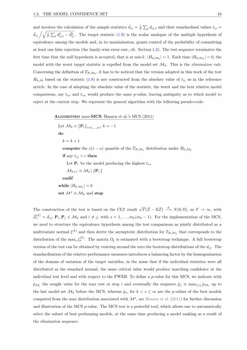
1.3. THE MODEL CONFIDENCE SET 16
and involves the calculation of the sample statistics dij = 1T
∑t dij,t and their standardised values tij =
dij
/√1T
∑t d
2ij,t − d2
ij . The target statistic (1.9) is the scalar analogue of the multiple hypothesis of
equivalence among the models and, in its maximisation, grants control of the probability of committing
at least one false rejection (the family-wise error rate, cfr. Section 1.2). The test sequence terminates the
first time that the null hypothesis is accepted, that is at min k : |H0,Mk| = 1. Each time |H0,Mk
| = 0, the
model with the worst target statistic is expelled from the model set Mk. This is the elimination rule.
Concerning the definition of TR,Mk, it has to be noticed that the version adopted in this work of the test
H0,M based on the statistic (1.9) is not constructed from the absolute value of tij as in the reference
article. In the case of adopting the absolute value of the statistic, the worst and the best relative model
comparisons, say tuv and tvu would produce the same p-value, leaving ambiguity as to which model to
reject at the current step. We represent the general algorithm with the following pseudo-code:
Algorithm max-MCS: Hansen et al.’s MCS (2011)
LetM0 ≡ Pii=1,...,m, k = −1
do
k = k + 1
compute the c(1− α) quantile of the TR,Mkdistribution under H0,Mk
if any tij > c then
Let Pr be the model producing the highest trs
Mk+1 ≡Mk\ Pr
endif
while |H0,Mk| = 0
setM? ≡Mk and stop
The construction of the test is based on the CLT result√T (Z − EZ)
d−→ N(0,Ω), as T → ∞, with
Z(k)s = dij , Pi,Pj ∈ Mk and i 6= j, with s = 1, . . . ,mk(mk − 1). For the implementation of the MCS,
we need to structure the equivalence hypothesis among the test comparisons as jointly distributed as a
multivariate normal ξ(k) and then derive the asymptotic distribution for TR,Mkthat corresponds to the
distribution of the maxs ξ(k)s . The matrix Ωξ is estimated with a bootstrap technique. A full bootstrap
version of the test can be obtained by centring around the zero the bootstrap distributions of the dij . The
standardisation of the relative performance measures introduces a balancing factor by the homogenisation
of the domain of variation of the target variables, in the sense that if the individual statistics were all
distributed as the standard normal, the same critical value would produce matching confidence at the
individual test level and with respect to the FWER. To define a p-value for this MCS, we indicate with
pMithe sought value for the max test at step i and eventually the sequence pj ≡ maxi≤j pMi
up to
the last model set Mk before the MCS, whereas ps, for k < s ≤ m are the p-values of the best models
computed from the max distribution associated withM?, see Hansen et al. (2011) for further discussion
and illustration of the MCS p-value. The MCS test is a powerful tool, which allows one to automatically
select the subset of best performing models, at the same time producing a model ranking as a result of
the elimination sequence.

17 CHAPTER 1. MODEL SELECTION FRAMEWORK
1.3.2 The t-MCS
With the second method we present in this study, we introduce the core argument by which novel MCS
tests are constructed. The intuition consists in assembling statistical tests that target the full collection
of pairwise model comparisons, whose outcome is exploited for the identification of the models that are
characterised by the MCS property 1.3.1. The main feature of our alternative tests is that of direct
model performance comparison, whereas in contrast the max -MCS hinges on the equivalence between
the model confrontation and the max statistics. The first contribution we provide is indicated as the
t-MCS, whereby we are inspired by the procedure presented in Corradi and Distaso (2011) and design
two variations of a new plain test of model multiple comparison. An application of the max -MCS and
the t-MCS to market risk model selection is presented in Cummins et al. (2017). From an operational
perspective, the MCS performs a random sequence of model benchmarking, whereby at each iteration
inferior models are rejected until all the surviving models are deemed equivalent. The rejected model set
may include the current benchmark, if inferior to any competitors. The following pseudo-code describes
the algorithm:
Algorithm t-MCS: Corradi et al.’s MCS (2011)
Let k = 0,M0 ≡ Pii=1,...,m, B0 ≡ ∅
do
pick any Pj ∈Mk\Bkcompute the tij , ∀i 6= j
call the relative performance test and let E ≡ Pu ∈Mk : Pu ≺ Pj
if there is a Ps ∈Mk : Ps Pj then
E ≡ E ∪Pj
endif
k = k + 1,Mk ≡Mk−1\E , Bk ≡ Bk−1 ∪Pj
whileMk\Bk 6≡ ∅
setM? ≡Mk and stop
The random benchmarking will generate a unique outcome if the decision rule is independent from the
sequencing. This can be achieved by considering a test statistic and hence critical values that remain
unchanged irrespective of the benchmark picking process. Nonetheless, the randomised sequence is not
strictly necessary for the construction of the test. In fact, if we consider all possible benchmark sequencing
we see that a model belongs to the MCS only if the collection of its expected relative performances are
significantly equivalent or superior to each and every competitor when it is either taken as the benchmark
or it is compared to a benchmark. By the symmetry of the tij ’s, the statistical preference rule that defines
the t-MCS leads to the same result whether the benchmark is Pi or Pj . Therefore, a model will enter
the MCS if and only if no dominant model can be identified. The t-MCS can therefore be simplified by
circulating the benchmark through M0 and rejecting the benchmarks that have at least one dominant
model, allowing the identification of the MCS in one single step. The pseudo-code for this modified
algorithm can be written as:

1.3. THE MODEL CONFIDENCE SET 18
Algorithm modified t-MCS
LetM0 ≡ Pii=0,...,m ,B−1 ≡ ∅
for k = 0 to m
compute tik ∀i 6= k
call relative performance test
if there is a Pi ∈M0 : Pi Pk then
Bk ≡ Bk−1 ∪Pk
else
Bk ≡ Bk−1
endif
endfor
setM? ≡M0\Bm and stop
In contrast to Corradi and Distaso (2011)7, we define the model preference rule by appealing to the CLT
for dependent sequences to construct asymptotic scalar tests for each relative model comparison. The
single fixed critical value Φ−1(1 − α), that is the α-right tail inverse cumulative normal distribution, is
exploited for the individual scalar relative model comparison test. This strategy allows control of the
confidence level for each scalar model comparison, but does not take into account test dependencies,
which are considered with joint model multiple comparison. This MCS test achieves model comparison
by either a random sequence or by a thorough cycle, which are equivalent procedures. As noticed at
the opening of this section, the approach we take with the analysis of the complete collection of model
confrontations is the building block of our alternative test, that in the forthcoming Section 1.3.3 is com-
bined with the generalised MHT framework to derive the novel γ-MCS. The t-MCS designed here, can
be considered as a streamlined version of that one, hinging on independent asymptotic statistics. In
this light, it will be interesting to compare the results of this test with those of the γ-MCS, which, as
presented below, employs the full arsenal of the MHT framework. Refining the t-MCS, we introduce a
ranking system for the MCS, a feature that cannot be produced by the original version of the t-MCS.
For this ranking system, we define the t-MCS p-value by taking the worst expected relative performance
for each model as determined by the bootstrap method and computing the complement of its quantile
on a standard normal distribution. This number represents the probability of committing a false rejec-
tion under the hypothesis of equivalence with its best competitor. Akin to the case of the max -MCS
p-value, the higher our t-MCS p-value the more confidence we have that a model is a member of the MCS.
We finally remark that for the max -MCS and t-MCS experiments pursued in this study, we compute the
sample statistics as bootstrap expectations, in order to render the testing results more robust to small
sample bias.
7 In Corradi and Distaso (2011) the authors chose√
2 log log T/T , a value that grants what they call a doubly consistentMCS, that is a model confidence set estimate which contains the “true” MCS with probability one and includes inferiormodels with probability zero.

19 CHAPTER 1. MODEL SELECTION FRAMEWORK
1.3.3 The γ-MCS
With the t-MCS introduced in the previous subsection, we have provided a test whereby the multitude of
hypotheses of the problem is central. The MCS is achieved with an algorithm employing scalar relative
performance tests. However, as anticipated, a limitation of this new elaboration is the disregard of the
dependency of the hypotheses. In this subsection, this alternative test construction is combined with
the general MHT approach to reconcile the multiple comparison nature of the model selection problem
with the MCS concept obtaining a new statistical test for the selection of the set of the best equivalent
models from a given model set of competitors. The proposed test can be seen as an extension to the
plain t-MCS device, which explores the model selection problem in a complete direct model contrasting,
taking into account the multi-hypothesis nature of the problem. The motivation for constructing an
alternative MCS test that takes into account test dependencies, can be found in the conjecture that the
MCS is not unique. This hypothesis is indirectly explored with the experimental exercises that have been
conducted in this thesis. Concerning the max -MCS, the solution provided exploits the correspondence
between the hypotheses set represented by the sequence H0,Mkand the multiple hypothesis Hij, pro-
viding also control for the FWER. This correspondence, however, holds asymptotically whereas small
sample distributions might not grant that an MCS constructed through the max statistic corresponds
to an MCS constructed with a statistical test exploring the whole combinations of pairwise comparisons
and furthermore controlling for the generalised k-FWER. In this thesis, we will learn through empirical
evidence that the latter conjecture is verified, providing further confirmation that the MCS is not unique
and, indeed, depends on the statistical procedure structuring the model preference ordering.
As an original contribution to the model comparison testing problem, we propose a new version of the
MCS test developed within the MHT approach, which achieves a further level of flexibility by allowing
balancing and strong control of k-FWER. Indeed, the intuition lies in noting that the construction of
the MCS corresponds to the identification of the models that are inferior to no other model. The setup
of the test has been anticipated in Section 1.2 when defining the test in (1.3), which is reproduced here
for the reader’s convenience. The MHT for the identification of the set of equivalent superior models is
structured as follows:
Hij : µij ≥ 0, ∀Pi,Pj ∈M0, i 6= j
which represents the complete set of the hypotheses8 of at least model equivalence to be submitted to the
testing framework. The rejection of the inferior models inM0 would leave the set of equivalent superior
modelsM?. A γ-TPFDP version of the MCS, which is coined γ-MCS, corresponds to the following steps,
as outlined in pseudo-code:
8 It is interesting to notice that the number of hypotheses that the construction of the MCS actually involves is waylarger than the number of modelsm. Therefore, allowing for flexibility in controlling for the k-FWER provides an additionalinstrument that permits to raise the tolerance above the model level rather than controlling for the false rejection of individualmodel comparisons.

1.3. THE MODEL CONFIDENCE SET 20
Algorithm γ-MCS: MCS with MHT controlling for the γ-TPFDP
LetM0 ≡ Pii=0,...,m ,B ≡ ∅
call the γ-TPFDP(α) procedure and
store the joint confidence set C
set B ≡ Pj ∈M : ∃ at least a Pi such that |Hij | = 0 with cij(1− α) < 0
setM? ≡M0\B and stop
In practice, the test is essentially made up of two steps: a first step where a γ-TPFDP(α) is run and
inference is jointly drawn about the model Pj ’s equivalence or superiority hypotheses Hij, that is the
generalised MHT on the full set of pairwise comparisons are progressively constructed until the loop
breaking condition of the FDP algorithm in Section 1.2.1 is reached9; a second step where the collection
of the outcomes is explored to search for rejection events, whereby the inferior models are identified and
dropped fromM0. The latter step is necessary because the MHT returns hypotheses on the individual
comparisons that must be searched in order to identify those elements that contradict the Definition 1.3.1.
As noticed in Section 1.2 each individual hypothesis is formulated as a right-tailed test, whereby the con-
jecture for the generic statistic tij is “model Pj is at least equivalent to model Pi”. Operationally, we
search for confirmation that the zero is at the left of the right hand boundary of the balance confidence
interval cij(1 − α). Were we to test equivalence10, we should control for the left hand boundary cij(α).
However, our effective target is the identification of the MCS, therefore after the MHT, we only need to
select the rejected hypotheses, which correspond to models that are inferior to at least another element
of M0. The correspondence is one-to-one as we are considering the full set of right-tailed hypotheses,
therefore targeting the model Pj , with the test statistic tij . Finally and to conclude the test, the proce-
dure moves from the test results to the model set B, by collapsing the hypotheses collection to the set of
models that have been rejected at least once. After the latter set has been removed from the initial model
setM0, we are left with the MCS, because the setM∗ does not contain any inferior models, therefore the
survivors must be all equivalent. The model setM∗, obtained as described, thus satisfies the definition
(1.3.1). With the γ-MCS, we are investigating the MCS as the remainder class, once the inferior models
have been eliminated. In fact,M0\B contains equivalent models that are at least equivalent to any other
model inM0. If that was not the case and the final set contained an inferior model, than the procedure
would yield a contradiction. On the other hand, if two models in the remainder were not equivalent then
either of the two would be an inferior model, yielding another contradiction.
Notwithstanding the superior statistical properties of the γ-MCS inherited from the MHT framework
9 If the implemented version requires a k-FWER that is set in advance, the γ-TPFDP loop is discarded and the algorithmruns directly the MHT with the target number of least amount of tolerated false rejections, with a given probability.
10 The choice of constructing the algorithm by targeting the right hand tails is a programming strategy, whereas analgorithm considering the (numerically more restricted) set of bidirectional hypotheses and therefore employing hypothesessuch as “models Pi and Pj are equivalent” could be employed, as well. The substantial difference would be that in ouralgorithm the distribution of the Jn in (1.6) involves the right tail of tij and its left tail through tji by merging them,whereas a two-sided test would keep left and right tails of tij distinct and there would not be the need of a tji statistic.In the latter case though, including the first or the second statistic would affect the distribution of k-minJn,j , ∀j andk-maxJn,j , ∀j and therefore change the outcome of the test, inducing non-uniqueness of the result. Avoiding the latterissue would entail the inclusion of both hypotheses of equivalence for tij and tji, therefore eliminating the problem ofwhich sequence of the orientation of the axis of the L’s characterises the set of equivalence. Nonetheless, another problemarises because under this configuration we would be duplicating the actual test hypotheses and therefore overstructuring therejection region. The solution employed for the construction of the γ-MCS entails no ambiguity for the region of rejectionand produces a unique bootstrap distribution of the multivariate statistic.
21 CHAPTER 1. MODEL SELECTION FRAMEWORK
which this construction relies upon, this procedure cannot produce either a ranking across the initial
and the rejected model sets, as it lacks an Holm-like sequence as in max -MCS. Exploiting the bootstrap
machinery, we resort to a wider definition of the MCS p-value, which, as opposed to the more conventional
MCS test, is independent from the algorithm that isolates the set of best models. We define the p-value
attached to model i by the γ-MCS as the probability of observing a relative model performance less than
zero, with respect to the probability distribution of the union of the events tij , ∀Pj ∈M? and represents
the probability of observing a superior performance of model i with respect to the model confidence set
M?. We notice that the target value represents the probability of model i to be included within the MCS,
as of the multivariate distribution of the model performance measures, estimated via the bootstrap. The
γ-MCS p-value contrasts with the max -MCS p-value taken out ofMk for model i, which represents the
probability of observing worst performances off the worst performance statistic TR,Mk, were the models
equivalent and compared at step k. The γ-MCS p-value is also different from the t-MCS p-value attached
to model i, as the latter represents the probability of observing worst performances of the benchmark i,
were it equivalent to its best performer, as identified by the bootstrap expectations. We notice further
that the latter two MCS procedures rely on asymptotic normal results, whereas the γ-MCS hinges on the
balanced bootstrap confidence sets and therefore it is expected to be more robust to non pivotal sample
distribution.
1.4 Thesis Summary
The last few decades have witnessed an increased complexity in the average model employed in the fi-
nancial industry. This complexity is continuing to rise and permeating all aspects of financial decision
making. Complex models are used not only in derivative pricing but are as well employed to measure
and control market risk, investment credit risk, counterparty risk, liquidity risk, and more. The potential
for operational risks resulting from the misuse, or worse from the misunderstanding of the functioning
of, a model is remarkable. In April 2011, the US Board of Governors of the Federal Reserve System
published the Supervisory Guidance on Model Risk Management (SR 11-7), which defines model risk
as the “potential for adverse consequences from decisions based on incorrect or misused model outputs
and reports”, Office of the Comptroller of the Currency (2011, p. 3). SR 11-7 typifies incorrect model
outputs, taking account of all errors at any point from design through to implementation. The European
Banking Authority’s Supervisory Review and Evaluation Process (SREP) requires that model risk be
identified, mapped, tested and reviewed. For this purpose, financial institutions have been structuring
internal model validation units in charge of the whole process of model risk evaluation. Among the many
aspects of model validation, one important step consists of the benchmarking of the chosen model, with
the ultimate objective of ranking the model set according to meaningful model performance measures. In
defining the tasks of model validation in Basel Committee on Banking Supervision (2009, p. 6), the reg-
ulator remarks that the valuation results should be confronted with an “independent benchmark model”.
Within this industry and regulatory context, the studies presented in this thesis would be of particular
interest to financial practitioners. We provide a statistically robust framework whereby model comparison
and hence selection can be performed within a systematised approach, which only requires the definition

1.4. THESIS SUMMARY 22
of the target model performance measure. With this thesis, we organise methods for model selection that
reduce the complex task of the comparison and ranking of models to a question of experimental design.
The experimental model selection exercises assembled and performed in this thesis provide new evidence
in applied statistics for finance. Drawing on the suite of methods set out in Section 1.3.1, Section 1.3.2
and Section 1.3.3, we tackle several model selection problems, applying relative model performance MHT,
the MCS and, through our methodological contribution, an MHT version of the MCS. The novel MCS
test allows to control the generalised k-FWER and further the γ-TPFDP. As we concentrate on largely
flexible model selection procedures, the subjects can be varied. We have decided to look at three typical
prototype problems in investment portfolios exposed to market risk, that is the estimation of several
portfolio risk metrics such as the VaR and the ExS, as well as the estimation of the historical and the
risk-neutral measures of widely employed stochastic processes in finance, such as jump-diffusion models.
The choice of these subjects of investigation is mainly related to the background of the author of this
manuscript, who has spent more than a decade working with applied econometrics in the wealth manage-
ment industry. We argue that these problems have an immediate appeal for practitioners. Nonetheless,
this choice is merely discretional as several other applications can be envisaged in the field of applied
econometrics. The following describes the layout of the thesis and sets out the main contributions of
each chapter, while highlighting a range of interesting findings that emerge. The concluding paragraphs
of this section summarise the evidence in relation to the comparison of the testing procedures that have
been implemented in this thesis.
In Chapter 2, we deal with the forecasting of some key measures in market risk management. These
are the value-at-risk and the expected-shortfall. We employ several econometric techniques to construct
market risk forecasting models that are confronted in an exercise similar to that of Bao et al. (2006).
The original contribution of our work lies in the application of generalised MHT and MCS techniques to
market risk forecasting model performance comparison. By means of the MHT framework, we provide
new evidence departing from the results of Bao et al. (2006), while at the same time delivering robust
inference for the identification of the best market risk models. While the MHT based tests from this
chapter have already been published in Esposito and Cummins (2015), post this publication, the analysis
for this chapter has been extended to include the construction of the max -MCS, t-MCS and γ-MCS. The
empirical results that we obtain diverge significantly from the evidence collected in Bao et al. (2006).
The target risk measures are the VaR and ExS forecast on 1-day and 10-day time horizons. We apply
model performance significance tests that are balanced and control for the k-FWER, with the auxiliary
benefit of the statistical power augmentation delivered by the step-down method. The absolute model
performance tests introduced with the MCS concept, have the ability to identify the subset of the best
performing models and produce a model ranking via the p-value measure, providing results that are
more informative than the RC p-value, which in Bao et al. (2006) fails to detect any model superiority
over the benchmark RiskMetrics model. In general, we find that models which account for volatility
mean reversion and fat-tailedness result in the best performance. This result is in contrast with previous
findings and shows that GARCH rolling window parameter estimates introduce high model uncertainty,
inevitably compromising their forecasting performance. The quantile regressions approach is shown to

23 CHAPTER 1. MODEL SELECTION FRAMEWORK
perform quite well. Model performance is generally found to be more widespread on longer horizons. The
expected-shortfall at 5% on a 1d horizon seems to be the most difficult to forecast, exhibiting the smallest
MCS. Historical Simulation, which is a common practice approach in industry, performs reasonably, re-
sulting in mid-ranking performance. Risk Metrics, another popular model among practitioners, does not
exhibit a noticeable performance and on the short term horizon enters the MCS only in the value-at-risk
at the 5% level.
In Chapter 3 we approach the problem of time-series estimation of jump-diffusion (JD) models, pro-
ducing experiments involving models of stochastic volatility and state dependent jumps with a latent
single-factor. In an important contribution, we investigate the model aliasing of structurally different
models, whereby model aliasing in our context is the observed behaviour that models, which have dis-
tinct dynamic features, nonetheless produce densities and estimates of the latent factor that are similar
and statistically exchangeable. In the same context, we develop a market data exercise that contributes
with experimental information to works such as Andersen et al. (2002), Chernov et al. (2003), Eraker
et al. (2003), showing, with the support of multiple comparison model selection procedures, that alter-
native models are able to produce superior model performances with parsimonious parametrisation. We
present a novel exercise of model selection applied to likelihood estimation and the latent factor filtering
with a JD model set acting on simulated and financial market data. We uniquely employ MHT and MCS
techniques to produce relative and absolute model performance comparison. Moreover, for estimation
purposes in our JD setting, we extend the second order filtering procedure in Maybeck (1982) to allow
jump components in the system state. The model set we consider contains the popular affine single
factor stochastic volatility model, augmented with a CEV parameter. The affine model is extended with
rare jumps in return under several specifications. The model set is extended with a stochastic intensity
high frequency jump class coupled with a constant volatility diffusion component, representing a non
standard alternative model family. The latter model class is taken into account as an alternative spec-
ification, whereby the volatility clustering is generated by means of mean-reverting stochastic intensity.
Both model families can include a jump in the latent affine factor, generating either stochastic diffu-
sion or stochastic intensity. Under simulated tests, the respective nesting models prove to be able to
produce similar features to one another, with respect to the performance measures. The latter result
reinforces the findings of the empirical exercise, whereby the stochastic intensity family exhibits superior
models in the majority of the tests. The strong conclusions that we are able to make from the analysis
is that there is a redundancy to jumps in volatility when measuring marginalised likelihoods, as well as
a non-significant prevalence of this component with respect to the latent component filtering measures.
The contribution of jumps in volatility appears to be dubious, contrary to the findings of Eraker et al.
(2003) and more in line with the model selection results of Chernov et al. (2003), though our findings are
more explicit than the latter. Secondly, high empirical kurtosis and moderate asymmetry are found to
be prevalent features, that can be captured with both conventional and non conventional models, that is
CEV with jumps as well as stochastic hazard models with high average frequency of jumps, with the latter
class performing slightly better under the filtering measures. Third, our findings point to the redundancy
of mixing both stochastic diffusion and stochastic intensity to model historical equity financial time series.

1.4. THESIS SUMMARY 24
Finally, with Chapter 4, we make a unique contribution through channelling, for the first time, the flex-
ibility and robustness of MHT and MCS methods to the problem of derivative pricing, whereby we test
different families of stochastic volatility models augmented with several types of jumps. The battery of
tests allow the comparison of option pricing models with respect to the mean squared pricing errors.
We employ a large sample of S&P 500 index options in our empirical analysis. We contribute to liter-
ature in several directions. We construct model comparison tests with novel MCS techniques targeting
a vast array of option pricing models, the majority of which result from original combinations of jump
and volatility specifications relative to the existing literature. This study provides empirical evidence of
strong aliasing amongst many option pricing models, ranging from high to lower levels of complexity.
This suggests scope for model simplification, which counters the trend in the academic literature towards
ever more complex derivatives pricing models. The model selection procedures we apply provide robust
evidence indicating that the popular single factor affine specification, extended in several directions, is
strongly rejected. Moreover, model augmentation such as jump in volatility, stochastic hazard and the
parametrisation of the elasticity of the diffusion factor are probably excessive complications. A simple
model, such as the correlated exponential volatility diffusion, perform very well in the OTM option sam-
ple, whereas the inclusion of a compensated single directional exponential jump in returns produces one
of the top performances for the ALL option sample.
In the Appendix A we provide technical details regarding the main algorithms developed throughout the
experimental parts and some proofs, whereas the Appendix B presents several algorithms in pseudo-code
that have been used for the experiments.
With respect to a thorough comparison of the flagship tests of this thesis, i.e. our version of the established
MCS test and our novel MHT based MCS, we remark that this task is beyond the scope of this work.
However, here we elaborate further as to why the MHT approach should be preferred. A first important
theoretical reason for our inclination towards the γ-MCS is certainly the lack of control for the generalised
FWER of the method of Hansen et al. As noticed in Romano and Wolf (2007), when the number of
tests in an MHT becomes large, control of the mere FWER becomes too stringent. In fact in the latter
scenario, the possibility of committing at least one false rejection grows to certainty, whereas controlling
at a high confidence level might force the test to accept a larger number of nulls. This reasoning led
the authors to a relaxation of the family-wise error concept, namely, the k-FWER. Another important
theoretical reason for preferring the MHT approach is represented by the concept of strong control of the
FWER as opposed to the weak control, the latter defined as the control of the FWER conditional on the
joint full set of hypotheses being true, whereas the former is referred to the conditioning on any subset
of hypotheses picked from the complete set. It is acknowledged that allowing for strong control might
be revealed as a formidable task. In the seminal paper Romano and Wolf (2005a), the authors point
out that the closure method of Marcus et al. (1976) can be used to construct methods that control the
FWER of the MHT Hi, i ∈ 1, . . . , k, if we know how to test each intersection hypothesis HK , which
denotes the hypothesis that all Hj are true, with j ∈ K and for any K ⊂ 1, . . . , k. This method can be
used together with the idealised method of Romano and Wolf (2005a) to construct a stepdown algorithm
that grants strong control of the FWER. From the perspective of this latter work, the MCS algorithm

25 CHAPTER 1. MODEL SELECTION FRAMEWORK
of Hansen et al. (2011) can be viewed as an idealised stepdown method, whereby the Tn,i statistics are
the max over all j models loss functions Li,j , for each benchmark model i, and the critical value cn,Ks is
the max statistic at iteration s for the set of surviving models Ks. In their seminal paper Romano and
Wolf point out that, with the purpose of avoiding the construction of 2k− 1 tests and allowing for strong
control, it is possible to construct k-order methods, provided that the theoretical statistic satisfies at
least the subset pivotality condition11 of Westfall and Troendle (2008) or the monotonicity condition12,
which is at the base of their bootstrap and subsampling construction of stepdown methods allowing for
strong control of the simple and generalised FWER. To the best of our knowledge, it is not clear if the
MCS of Hansen et al. (2011) grants for strong control of the FWER13. The latter should be the topic of
more focused future research.
In more practical terms, what we have achieved in this thesis, with regard to the confrontation of the two
MCS methods, is the collection of qualitative evidence. We have encountered diverse circumstances. In
the market risk forecasting exercise of Chapter 2, the model set elements achieve moderately homogeneous
performances, at least on the one day horizon, allowing the max -MCS and the γ-MCS to isolate the
cluster of best models. The MHT based test can furthermore modulate the sensitivity to false rejections
and incrementally reduce the model confidence set, which exhibits sensitivity to this parameter. Higher
tolerance to false discovery shrinks the MCS toward the t-MCS outcome, which in general manifests a
more aggressive outcome, providing a more restricted MCS in the majority of the experiments. When the
model comparison is more ambiguous as in the ten day market risk forecast horizon or in the artificially
generated model aliasing of the jump-diffusion model estimation experiments of Chapter 3, all of the
MCS tests struggle to identify the best model set, although the γ-MCS provides a more informative
model ranking measure, while the t-MCS results in a tighter selection. The latter test might be useful
as a quick diagnostic tool to identify the region containing the candidate best models or in conditions
where it is difficult to distinguish models, the t-MCS might provide a term of comparison for various γ
values in the γ-MCS. The behaviour of the tests in the market data experiment of the jump-diffusion
model estimation exercise presents a condition where all the statistics agree upon the size of the MCS. In
this case, the MCS is pretty much insensitive to the γ-TPFDP controlling parameter. Finally, in the last
chapter, Chapter 4, of this thesis we are confronted with a very large option pricing model set experiment,
whereby the model components are shown to perform very closely to one another. In this exercise, the
ability of the γ-MCS to modulate the result by targeting different k-FWER allows one to focus upon
the set of best performing models, whereas the benchmark test max -MCS is incapable of providing any
screening of the large option pricing model set, failing to reduce the initial set at a 10% confidence level.
This is an interesting outcome that shows the limitations of the max -MCS in the presence of a large model
set and should be connected to the control of the simple FWER, which is revealed to be too stringent is
such a context. A further indication of this relation can be found in the ability of the γ-MCS to restrict
11 The subset pivotality condition states that, heuristically, the statistic joint distribution that is used to test the subsetof true hypothesis is not dependent on the truth or falsehood of the remaining hypotheses.
12 The monotonicity condition is satisfied if the algorithm is such that, given the set J contained in set K, J ⊂ K, thenthe critical values produced by the algorithm cn,J and cn,K associated, repectively, with the set J and K, are such thatcn,J ≤ cn,K .
13 It has to be noticed that in Romano and Wolf (2005a), the authors remark that the reality check of White (2000),which might be seen as a subcomponent of the MCS test, allows for the weak only control of the FWER.
1.5. CONCLUDING REMARKS 26
the final set by relaxing the number of allowed false rejections at the target confidence level. Moreover, as
the MHT based MCS permits the direct testing of the complete set of model comparisons by constructing
specific confidence intervals, a more granular check of the order of precedence is possible, whereby in a
tightly competing model set, several model contrasting measures might be close to the rejection tail and
the triggering of the k-FWER would allow the user to expose these borderline behaviours. A further point
of comparison can be identified in the behaviour of the p-value, that in the case of the max -MCS exhibits
the tendency for a lack of discriminating capacity between the top section of the MCS components. This
feature might be related to a finite sample distribution bias, a characteristic that has not been explored.
Ultimately, the p-value model ranking measure that we construct for our novel test, provides a highly
significant ranking factor that does not produce the counterintuitive result of the max -MCS’s p-value.
1.5 Concluding Remarks
In this chapter we have defined the model selection framework to be used in the applied econometrics
exercises of the following chapters, whereby we have specified the notion of significance of the model
performance, relative and absolute model comparison. In the following chapters we produce statistical
experiments of the latter type. Furthermore, we have introduced the multiple hypothesis testing frame-
work and defined the model confidence set. With respect to the latter concept, we design a MCS test
with the Hansen et al. (2011) approach, the max -MCS and introduce two alternative novel tests, the
t-MCS and the γ-MCS. Both tests hinge on the full collection of the pairwise comparisons of the model
set components. In the first procedure, the test dependencies are disregarded and each model comparison
is dealt with as an individual scalar test hinging on CLT results. With the second procedure, the major
contribution of this chapter, we combine the MCS concept with the arsenal of the MHT approach, pro-
ducing a novel MCS test relying on non pivotal results, which exploit balanced confidence sets and allows
strong control for the k-FWER. In the course of this thesis, the latter innovation provides an important
means of refinement of the initial model set.

27 CHAPTER 2. MODEL SELECTION OF MARKET RISK MODELS
Model Selection of
Market Risk Models
Value-at-Risk, or more simply VaR, has gained popularity among practitioners in the past years
because of the increasing exposure to market risk of large financial companies and financial divisions
of non-financial firms, and mostly because of the ability of this metric to deliver a readable quantity
concerning overall risk borne. This popularity has increased as a result of the many “crises” and large
corporate defaults due to market exposure, which have become more frequent since the early 90’s and
largely publicised by the media. VaR1 is used by risk managers in banks and wealth management compa-
nies to monitor the market risk of large and varied portfolios of financial securities and over-the-counter
products in order to trigger action by the management on the back of the information packed into this
number. This metric summarises the optimistic loss in a worst case scenario, with a given probability on
a certain time horizon. This calculation has also become part of regulatory requirements, e.g., in banking
regulations such as in Europe, whereby it is used to determine the amount of regulatory and economic
1 We keep referring to VaR in this work although we always mean the target quantile of the empirical returns. Nevertheless,originally, the VaR is defined as a monetary measure that better refers to a consolidated portfolio of asset values ratherthan returns. However, it is theoretically easy to switch from one measure to another.

28
capital. From an operational point of view, however, VaR in general lacks the important property of
subadditivity, Artzner et al. (1999). Practically, this means that the VaR of a weighted sum of individual
quantities is not equal to the weighted sum of each VaR, hence requiring multiple layers of calculation
when aggregating from subsets to the consolidated portfolio level. This feature led to a shift of focus
towards the alternative risk measure of expected-shortfall (ExS), see Artzner et al. (1999), which holds
the subadditivity property and provides further information: namely, the expected loss in a worst case
scenario, with a given probability on a certain time horizon. This measure represents also a complemen-
tary indicator that accounts for the magnitude of losses exceeding the VaR threshold and draws attention
to the full shape of the tail event distribution.
The statistical testing of risk models is an important step towards assessing the ability of these tools to
provide reliable output and to contribute to the decision-making process hinged on market risk exposure.
From a practitioner perspective, there are serious implications for a financial institution from its choice
of risk model in terms of its overall risk management performance and more importantly its capital ad-
equacy requirements. So for industry, the question of which risk model performs bests in capturing and
forecasting risk exposure is crucial. Historically the first contributions in backtesting the performance
of risk-models are those of Kupiec (1995) and Christoffersen (1998), who construct unconditional and
conditional tests based on the mere sequence of VaR breaches. Thereafter, research focused on specific
issues affecting the VaR prediction ability, such as the time-horizon of the forecast, the inclusion of time-
varying volatility and accounting for fat-tailed distributions generated by volatility clustering and jumps
in returns, see BIS (2011) for a review. On the other hand, backtesting ExS is more problematic due to
the peculiarity of its functional form which in principle requires the estimation of the entire tail distri-
bution. The literature on model prediction of ExS is not as extensive as that on VaR, possibly due to
the latter reason. The main contributions in this field are Berkowitz (2001) and Kerkhof and Melenberg
(2003), who use the probability transform Rosenblatt (1952) to process the data and construct tests of
ExS prediction based, respectively on the likelihood ratio and the δ-functional method Van der Vaart
(1998). Both these works focus on the development of a test for ExS.
In this chapter, we build on the work of Bao et al. (2006) in that we use a similar model set but investi-
gate model predictive ability not only for the VaR but also for the ExS models with respect to different
time horizons and volatility conditions. The main contribution of this work consists of the application
of the MHT framework to the backtesting of market risk measures. We test the statistical significance
of the forecasting performance of a varied set of market risk models, targeting the VaR and the ExS risk
metrics. We design MHT exploiting the empirical coverage probability as the sample statistic for the
VaR, whereas we use the sample shortfall as we develop a new test of significance and model comparison
for the ExS. Moreover, in this thesis, we extend the already published work (Esposito and Cummins,
2015), aiming our sights at the absolute model comparison of market risk forecasting models. Employing
the methodological approach developed in Section 1.1 and Section 1.3, we designed MCS tests of the
market risk absolute model performance hinging on the max -MCS of Hansen et al. (2011), as constructed
in Section 1.3.1, our new t-MCS inspired by Corradi and Distaso (2011), as constructed in Section 1.3.2,

29 CHAPTER 2. MODEL SELECTION OF MARKET RISK MODELS
and the novel γ-MCS, as constructed in Section 1.3.3, settling the MCS in an MHT framework2.
We construct bootstrap MHT of risk model predictive ability, analysing the out-of-sample performance
over 1-day and 10-day time horizons. We extend the investigation to forecasts that target a time hori-
zon wider than a single day, an exercise that might either confirm the predictive power of a model or
highlight situations whereby the forecast deteriorates fast. We also observe the model performance under
stressed market scenarios. The inference procedure is accomplished via a direct measure of the VaR
predictive ability or rather exploiting the idea first popularised by Diebold et al. (1998) and used by
Berkowitz (2001), Kerkhof and Melenberg (2003), Bao et al. (2007), in that we use the probability trans-
form Rosenblatt (1952) to construct statistics which are functionals of the model probability distribution
and thereby indirectly test the data via the probability transformed sample. The battery of tests draws
inference about two aspects of the model forecasting ability. In a first exercise, we construct tests of
statistical significance of the forecasting ability of each model, with reference to the target quantities to
be predicted. The latter can be easily recognised in the VaR forecasting test, whereas in the ExS test
we resort to pre-pivoting to obtain a data domain standardisation and construct a new simple test for
the backtesting of the model predictive ability of the expected-shortfall. With this backtesting exercise,
we estimate confidence sets for the target statistic and derive joint balanced tests which control for the
k-FWER. This experiment also presents an application of the streamlined step-down algorithm, as pre-
sented in Section 1.2.2, a procedure of recursive testing that potentially allows for further rejections,
in an attempt to increase the statistical power of the test. In a second application, we explore model
superiority in market risk forecasting with an absolute model performance test. We derive the max -MCS,
the t-MCS and the γ-MCS.
The chapter is organised as follows. In Section 2.1 we briefly introduce the conditional distribution models
that form the suite of competing market risk forecasting instruments, whereas in Section 2.2 we define
the target risk measures and the sample statistics, further describing the structure of the testing exercise.
The experimental Section 2.3 describes the data set, the modelling approach and discusses the empirical
evidence exhibited. This section also introduces the first application of the MCS tests providing some
examples of the operational characteristics of the model confidence set tests. Section 2.4 concludes.
2.1 The Conditional Distribution Model Set
In this chapter we introduce the components of the market risk forecasting model setM. The output of
the models we are interested in is the conditional probability density forecast delivered by the different
techniques. Although it is sufficient to model just the tail of P to produce the inference that is sought,
in certain cases we will need the full distribution to project the system forward. The model set includes:2 In a previous version of this analysis, we approach the absolute model comparison by exploring the bootstrap generated
multidimensional distribution of the model performances, measuring the probability that each Li ≤ Lj of pairwise superior-ity, for each dij . This information is then collated into a synthetic table presenting a model ranking index that represents,for each model, the number of time this probability is greater than 0.5, providing an instrument for measuring the modelsuperiority across the model set. In this work we do not present this information as it resemble the results of the absolutecomparison test we are introducing, whereas the statistical properties of the latter approach have been extensively studiedin the literature.

2.1. THE CONDITIONAL DISTRIBUTION MODEL SET 30
heuristic models such as the historical simulation (HS), which is a rolling window histogram, a rolling
window Normal model (G) and RiskMetrics (RM)3; a non-parametric model based on a kernel regression
(KR); parametric models such as the autoregressive conditional heteroskedastic model (CH), the quantile
auto-regression model (QR) and several parametric distribution assumptions such as normality, student-t,
generalized error distribution (GED) and the generalised Pareto distribution (GPD).
Historical Simulation
The historical simulation (HS) model consists of a rolling window histogram of the return distribution.
The implicit assumption is that a t-left neighbourhood data sample histogram is a good local estimate of
the conditional distribution Pt. Although this might be acceptable as an estimate of Pt (Xt+ε) , ε > 0,
a model-free approach seems inadequate when ε 0. Under the i.i.d. assumption, we can compute the
distribution ∆ lags forward with numerical convolution or Monte Carlo integration. This model is the
most widespread in the financial community, because of the ease of implementation and mainly because
it allows one to aggregate easily the many varieties of financial exposures which would otherwise require
the design of an all-inclusive market risk model.
Normal Hypothesis
The classical assumption of the Black-Scholes model is that log-returns are normal. A practical approach
to the estimation of a conditional mean-variance model is the plugging in of a rolling window sample
mean and variance into the normal function to construct a model of Pt (Xt+ε). This model should be
able to capture some momentum and volatility clustering.
RiskMetrics
The RM model, J.P.Morgan (1996), consists of an exponential smoothing of the squared returns, which
is used for a t+ 1 variance proxy. Formally,
ht = θ · ht−1 + (1− θ) · x2t−1. (2.1)
It was originally designed as a simple alternative to the GARCH model on the observation that the lag
polynomial is often close to the stability condition and the GARCH parameters for financial time series
are not widely different across a large collection of data. It presents the disadvantage that it cannot be
projected forward. As a working template, we use the normal hypothesis to compute projections of the
conditional probability distribution, assuming innovation of the variance proxy at current h.
Kernel Regression
A robust and efficient (but biased) technique to estimate a conditional distribution is to exploit the
kernel regression of Nadaraya-Watson, cfr. Nadaraya (1964), Watson (1964) and Bierens (1987) for
3 The RiskMetrics model is presented as a heuristic model because the model parameter θ is fixed a-priori and we assumeconditional normality to project the system forward.

31 CHAPTER 2. MODEL SELECTION OF MARKET RISK MODELS
several statistical results. Formally,
Ey|x =
∑j yjKh(x− xj)∑j Kh(x− xj)
(2.2)
A drawback of this estimator is that it shows high variability when conditioning on values of xt−∆ that
are far away from the centre of gravity of the sample distribution, therefore producing unstable estimates
of the tails. On the other hand, an attractive feature of the KR estimator is that it can generate directly
an estimate of the distribution conditional on any lag; in this case the projection exercise is a direct
output of the estimation function.
Quantile Regression, CAViaR
The quantile regression model, Koenker and Bassett (1978), is a statistical model of empirical percentile.
Basically, it is a parametric model of relations between the explanatory variables and the percentile of
the target variable. In this work, we employ the specification in Engle and Manganelli (2004), which
accounts for autoregressive features of the model quantile. The model has been designed pretty much
for the estimation of an auto-regressive VaR, therefore the epithet of conditional autoregressive VaR,
designated as CAViaR. Formally, letting Xt−1 = yt−1, . . . , yt−i, . . . , a quantile auto-regression model
is defined as
yt = f (Xt−1;β) + εθt
= ft (β) + εθt ,
with the auxiliary assumption that the θth-quantile of the εθt distribution is equal to 0. The model
estimation is carried out with the minimisation of the loss function
minβ
1
T
∑t
(θ − 1yt<ft(β)
)(yt − ft(β)) (2.3)
which is minimal whenever ft ≡ θ.
In this work we employ four different CAViaR specifications: the adaptive; the symmetric; the asymmet-
ric; and the indirect GARCH. The latter three models are specified as in Engle and Manganelli (2004),
whereas the adaptive CAViaR is defined as
ft = ft−1 +[1yt−1<ft−1 · b1 + 1yt−1≥ft−1 · b2
]· (yt−1 − ft−1). (2.4)
For each model, we estimate a quantile regression for the 1st-5th percentiles, in addition to the 7.5% and
10% levels, in order to smooth out the borders of the distribution. Hence, we use those percentiles as
a point-wise tail estimate. The extreme value distribution is assumed to have a linear to higher order
polynomial decay, matching the all-time minimum, with polynomial degree ranging from 1 to 20. In this
exercise we are modelling the tail of the conditional distribution function only. We project the distribution
forward, simply multiplying the knot points, that is the estimated percentiles, by the square root of time.

2.2. MODEL COMPARISON TESTING 32
GARCH-EVD Models
Financial time series exhibit volatility clustering features and fat tailed distributions. The generalised
autoregressive conditional heteroskedastic models, Engle (1982), Bollerslev (1986), represent the most
successful statistical device in mimicking the evolution of financial time series in the past thirty years.
The GARCH models come in a variety of fashions. However, a GARCH(1,1) does not seem an unrea-
sonable assumption for financial time series, cfr. Hansen and Lunde (2005). In the MHT experiment
we account for modelling time series volatility clustering with conditional heteroskedastic models, and
incorporate asymmetry with exponential or threshold GARCH, cfr. Nelson (1991) and Glosten et al.
(1993). Specifically, we estimate symmetric GARCH models, Engle (1982), Bollerslev (1986)
ht = α0 + α1ε2t−1 + β1ht−1 (2.5)
and models capable of producing asymmetric distributions such as the TARCH(1,1) of Glosten et al.
(1993)
ht = α0 +(α1 + γ1εt−1<0
)ε2t−1 + β1ht−1 (2.6)
and the EGARCH(1,1) of Nelson (1991)
log ht = α0 + α1 (|vt−1| −E |vt−1|) + β1 log ht−1, (2.7)
with εt = vt√ht.
The stochastic driver vt is such that Evt = 0, Ev2t = 1 and vt ∼ G(θ), where G(θ) is a parametric
distribution of type normal or student-t. However, it is common knowledge that financial time series
exihibit fat tailed4 distributions, Longin (1996). Further improvement is achieved by augmenting the
model with a piecewise distribution for G(θ). Thereby, we adapt extreme-value distributions to each tail
of the residuals with a quasi-maximum likelihood estimation (QMLE) of the model classes introduced
above, while a conditional normal or GED is estimated for the mid percentiles. In order to parametrise a
GPD for each tail, we exploit the idea in Gonzalo and Olmo (2004) and maximise the Kolmogorov-Smirnov
statistic of the empirical distribution of the exceedances. This approach is different from that taken by Bao
et al. (2006), whereas the threshold is picked at a conventional level. A robust alternative semi-parametric
estimation technique has been proposed in Mancini and Trojani (2011). The described econometric setup
is able to capture the time dependency described by volatility clustering, the asymmetric effect and the
thick tails phenomenon.
2.2 Model Comparison Testing
The design of tests of market risk model forecasting performance requires the determination of the
target risk measures employed with the loss functions L. The target risk measures are the VaR and
4 When we refer to fat-tailedness in this thesis, we refer to model distribution tails that are not exponentially boundend.High kurtosis, on the other hand, is a measure of the distribution shape that can be referred to as the “peakedness” of thedistribution. The kurtosis might be affected by fat-tailedness.

33 CHAPTER 2. MODEL SELECTION OF MARKET RISK MODELS
the ExS5. In this regard, it is important to notice that in this chapter we refer to the VaR measure as
obtained under the log-transform of the price, which is therefore the corresponding quantile of the return
distribution forecast. Under a monotonic transformation, quantiles are preserved. However, this is not
true for the ExS, which is thus the expected shortfall of the portfolio return, not the value. Formally, let
Ft,∆(x) := Pt (Xt+∆ ≤ x) and define the value-at-risk
VaRt(∆, α) = F−1t,∆(α) (2.8)
that is the α percentile of the return conditional distribution over the target time horizon ∆, and the
expected-shortfall
ExSt(∆, α) = 1αEPt
[Xt+∆1Xt+∆<VaRt(∆,α)
]. (2.9)
that is the return expectation, conditional upon observing values below the VaRt(∆, α). The correspond-
ing sample measures of the quantities defined in (2.8) and (2.9) are either employed in the construction
of simultaneous confidence set for the statistical significance test or enter the loss function defined as the
absolute difference between the realised values and their ex-ante expectations. The type of tests we set
up concern the model forecasting ability of VaR and ExS over 1-day and 10-day time horizons, under low,
high and average volatility conditions. We test the VaR model predictive performance, cfr. Bao et al.
(2006), Kerkhof et al. (2009), using the sample measures of the empirical coverage probability (ECP).
Assuming a sample of T observations, starting from the first datum after the minimum amount of data
needed for the estimation, we define the ECP as
ρ := 1T−∆+1
T∑t=∆
1Xt<VaRt−∆ (2.10)
To obtain tests targeting the expected shortfall, we transform the data with the ∆-step ahead conditional
distribution Pt (xt+∆) to construct the probability transform yt+∆ =∫ xt+∆
−∞ dPt(s; ∆), obtaining the ran-
dom variable Y that is independent uniformly distributed, cfr. Rosenblatt (1952), Diebold et al. (1998).
Exploiting the sequentially independence property of Y , the latter work derives tests for probability
density forecasting performance whereby the loss function measures the divergence of the transformed
data from the uniform distribution. Building on this approach, several formal methods of testing density
forecasts and applications to financial risk measurement have been designed, based on the likelihood-ratio
test, cfr. Berkowitz (2001), the Kullback-Leiblier information criterion, cfr. Bao et al. (2007) and the
δ-functional method, cfr. Van der Vaart (1998) and Kerkhof and Melenberg (2003). In this study instead,
we apply the probability transform and then derive the sample measure
ρ :=
∑Tt=∆ Yt1Yt<ν∑Tt=∆ 1Yt<ν
(2.11)
where ν indicates the reference percentile of Y , with respect to the sought shortfall. It is appropriate for
a forecasting model selection exercise defining the loss function Li of model i for the various measures as5 To be rigorous, see e.g. Kerkhof and Melenberg (2003), the VaRt(∆, α) might have a finite probability (P not sur-
jective) or an interval on X might have 0 probability (P not injective). In the most general definition, VaRt(∆, α) :=
inf x ∈ R : Pt (Xt+∆ ≤ x) ≥ α and ExSt(∆, α) :=EPt [Xt+∆|E ]+[Pt(E)−Pt(E)]·VaR∆,α
Pt(E)with E = Xt+∆ < VaRt(∆, α).
However, this extended definition is redundant for operational purposes.
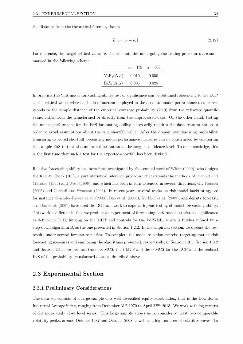
2.3. EXPERIMENTAL SECTION 34
the distance from the theoretical forecast, that is
Li := |ρi − ρ∗| (2.12)
For reference, the target critical values ρ∗ for the statistics undergoing the testing procedures are sum-
marised in the following scheme:
α = 1% α = 5%
VaRt(∆,α) 0.010 0.050
ExSt(∆,α) 0.005 0.025
In practice, the VaR model forecasting ability test of significance can be obtained referencing to the ECP
as the critical value, whereas the loss function employed in the absolute model performance tests corre-
sponds to the sample distance of the empirical coverage probability (2.10) from the reference quantile
value, either from the transformed or directly from the unprocessed data. On the other hand, testing
the model performance for the ExS forecasting ability, necessarily requires the data transformation in
order to avoid assumptions about the true shortfall value. After the domain standardising probability
transform, expected shortfall forecasting model performance measures can be constructed by comparing
the sample ExS to that of a uniform distribution at the sought confidence level. To our knowledge, this
is the first time that such a test for the expected-shortfall has been devised.
Relative forecasting ability has been first investigated by the seminal work of White (2000), who designs
the Reality Check (RC), a joint statistical inference procedure that extends the methods of Diebold and
Mariano (1995) and West (1996), and which has been in turn extended in several directions, cfr. Hansen
(2005) and Corradi and Swanson (2006). In recent years, several works on risk model backtesting, see
for instance Gonzales-Rivera et al. (2003), Bao et al. (2006), Kerkhof et al. (2009), and density forecast,
cfr. Bao et al. (2007) have used the RC framework to cope with joint testing of model forecasting ability.
This work is different in that we produce an experiment of forecasting performance statistical significance
as defined in (1.1), hinging on the MHT and controls for the k-FWER, which is further refined by a
step-down algorithm B, as the one presented in Section 1.2.2. In the empirical section, we discuss the test
results under several forecast scenarios. To complete the model selection exercise targeting market risk
forecasting measures and employing the algorithms presented, respectively, in Section 1.3.1, Section 1.3.2
and Section 1.3.3, we produce the max-MCS, the t-MCS and the γ-MCS for the ECP and the realised
ExS of the probability transformed data, as described above.
2.3 Experimental Section
2.3.1 Preliminary Considerations
The data set consists of a large sample of a well diversified equity stock index, that is the Dow Jones
Industrial Average index, ranging from December 31st 1970 to April 22nd 2013. We work with log-returns
of the index daily close level series. This large sample allows us to consider at least two comparable
volatility peaks, around October 1987 and October 2008 as well as a high number of volatility waves. To

35 CHAPTER 2. MODEL SELECTION OF MARKET RISK MODELS
perform the backtesting experiment, we split the data sample into in-sample and out-of-sample segments,
assuming size T = R+P , where R indicates the size of the in-sample data used for model estimation and
P indicates the size of the sample used for prediction in the out-of-sample segment. The full sample size
is T = 10, 674. The working assumption here is that there exists stable transition probability distribu-
tions, albeit unknown. We subtract the sample average from the return sub-sample ending on December,
31st 1998, assuming thereon a zero off-set constant. We draw on a large sub-sample for first estimation
and set R = 6, 572, that is we start the out-of-sample exercise on January, 1st 1997 and use the same
parameters for the parametric models throughout 260 observations, after which the model is estimated
again. As a consequence we split the out-of-sample exercise into 16 blocks which are re-sampled 2,000
times with the stationary bootstrap of Politis and Romano (1994b). We choose the sample size such
that we observe sensible smoothing of the statistic distributions. The optimal bootstrap block-length is
estimated on the growing sample base with the Patton et al. (2009) algorithm. We deliberately discard
the rolling-window approach for parametric models like GARCH-EVD and CAViaR because this practice
increases rather than shrinks the forecast variability. For instance, the autoregressive coefficient of the
symmetric GARCH equation exhibits wide variations if resulting from a two-year rolling sample monthly
estimate as opposed to the procedure employed in the experiments consisting of a yearly estimate on a
growing sample basis. For reference, the mentioned rolling-window approach for a symmetric GARCH
model would produce an average autoregressive coefficient of 0.869 with a standard deviation of 0.073 and
a spike at 0.346, whereas the growing sample approach delivered an average coefficient of 0.920 with a
standard deviation of 0.002. We believe that is the main reason for the poor performance of the GARCH
models in, e.g., Kerkhof et al. (2009) and Bao et al. (2006). Hence, in this study we do not include rolling
window versions of the GARCH or CAViaR models, relying on the results of similar models employed
by other authors for reference. The rolling window approach applied to models that are designed to
produce conditional and stationary distributions of the data generating process, is more likely to hurt
their performances by the increased model uncertainty introduced with the parameter variability, rather
than improving their local forecasts. Concerning the estimation risk, we adopt the working hypothesis
that the parameters or the non-parametric estimates are set to their p-limits, due mainly to restrictions
to the currently available computational power. We plan to expand this feature in future experiments
and include estimation risk in the full simulation.
In this empirical study, we generate the sample statistics with resampling from subsamples of 260 days.
There are two reasons for this: firstly to avoid the phenomenon of location bias, Corradi and Swanson
(2007), that is the bias in resampling for recursive problems, whereby earlier observations are used more
frequently than temporally subsequent observations when forming test statistics; and secondly to con-
struct artificial samples with classified volatility, in order to investigate the model performance in different
volatility environments. The average block size for the resampling procedure is computed according to
the Patton et al. (2009) procedure, resulting in a 195 day block size. We construct model predictive
ability measures on 1-day and 10-day projections of the target risk measures, the latter time-horizon
corresponding to 2-weeks of calendar days. The risk measures presented in this report are the empirical
coverage probability, for VaR models, and the realised ExS of the probability transformed sample distri-
butions. However, the analysis has been performed on a slightly larger set of measures, containing the

2.3. EXPERIMENTAL SECTION 36
empirical loss function and the VaR of the pivoted sample, essentially producing the same results. As
described earlier, the out-of-sample data is divided into 16 blocks of 1 calendar year.6 We investigate the
full out-of-sample performance of the models. Furthermore, we back-test the performance in low / high
volatility scenarios each corresponding to four blocks labelled as L/V and H/V, representing extreme
sample years. The blocks are not necessarily time-contiguous.
Where necessary, the model 1-step and 10-step distributions are constructed via Monte Carlo integration.
In order to consistently reduce the computational time, the GARCH-EVD distributions are constructed
on a grid for the conditioning variable entailing an array of forecast distributions, which is used at run
time by truncating over the prescribed grid the dependency on the current value. The historical simu-
lation is projected forward via Monte Carlo integration. The RiskMetrics distributional assumption is
Gaussian with ht variance. The Kernel regression estimate is constructed in a similar manner as the
GARCH-EVD distributions, that is on a grid for the conditioning variable that is determined on the
historical sample as well. In order to reduce the computational time, the Kernel regression is also kept
fixed until the subsequent estimation. The rolling window models are recalculated daily at time t−1. The
CAViaR equation requires some inventiveness to be employed. As they stand, the quantile regressions
cannot be projected forward or input in the probability transform, because they have naturally been
designed to be free of any distributional assumption. This model is appealing both for the short term
memory quantile feature as well as for the absence of an explicit probability assumption. Nevertheless,
we need a conditional distribution to feed the Rosenblatt functional and construct the ExS backtesting
procedure. Therefore, we proceed by estimating several quantile auto-regressions to construct a linear
approximation of the tail of interest. We need to expand on the inner side in order to avoid polarisation
on the quantile of interest, that is the 5th in this exercise. Meanwhile, on the outer side, we need a
tail assumption to work with. We start joining the all time minimum with the first percentile with a
straight line and then with a (translated and scaled) polynomial of degree 5, 10 and 20. To be sure that
the operation model we are designing produces reasonable results, we ought to prove that the percentile
order is what is expected to be. In this case, we rely on the careful choice of the pivot points, on the
constraint preventing the autoregressive quantiles to cross each other, were that to happen and, of course,
on the empirical evidence. The quantiles are carried forward in time simply multiplying by the square
root of time.
Furthermore, we are also interested in the significance of conditioning in the presence of model misspec-
ification. We include in the model a fully unconditional distribution assumption, based on a dual tail
GPD distribution with constrained normal or GED distribution for the mid quantiles, estimated through
MLE on the base sample. We also consider for the 10-step ahead forecast the unconditional distribution
of the GARCH-EVD models. This distribution is constructed taking the expectation with respect to the
conditioning variable, formally P(X) = EY [P(X|Y )], which corresponds to the k-step unconditional dis-
tribution under the modelling specification. The rationale in testing these models relies on the possibility
that the forecast 10 steps ahead is possibly distorted by the conditioning, firstly because of the speed
of the mean reversion of the volatility, which should be ruled out by the preliminary tests on the model
6 The last block is less than 1 year but the resampled data is let run for a full year.
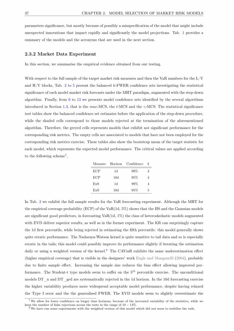
37 CHAPTER 2. MODEL SELECTION OF MARKET RISK MODELS
parameters significance, but mostly because of possibly a misspecification of the model that might include
unexpected innovations that impact rapidly and significantly the model projections. Tab. 1 provides a
summary of the models and the acronyms that are used in the next section.
2.3.2 Market Data Experiment
In this section, we summarise the empirical evidence obtained from our testing.
With respect to the full sample of the target market risk measures and then the VaR numbers for the L/V
and H/V blocks, Tab. 2 to 5 present the balanced k-FWER confidence sets investigating the statistical
significance of each model market risk forecasts under the MHT paradigm, augmented with the step-down
algorithm. Finally, from 6 to 13 we presents model confidence sets identified by the several algorithms
introduced in Section 1.3, that is the max -MCS, the t-MCS and the γ-MCS. The statistical significance
test tables show the balanced confidence set estimates before the application of the step-down procedure,
while the shaded cells correspond to those models rejected at the termination of the aforementioned
algorithm. Therefore, the greyed cells represents models that exhibit not significant performance for the
corresponding risk metrics. The empty cells are associated to models that have not been employed for the
corresponding risk metrics exercise. These tables also show the bootstrap mean of the target statistic for
each model, which represents the expected model performance. The critical values are applied according
to the following scheme7,
Measure Horizon Confidence k
ECP 1d 99% 3
ECP 10d 95% 4
ExS 1d 99% 4
ExS 10d 95% 5
In Tab. 2 we exhibit the full sample results for the VaR forecasting experiment. Although the MHT for
the empirical coverage probability (ECP) of the VaR(1d, 5%) shows that the HS and the Gaussian models
are significant good predictors, in forecasting VaR(1d, 1%) the class of heteroskedastic models augmented
with EVD deliver superior results, as well as in the former experiment. The KR can surprisingly capture
the 1d first percentile, while being rejected in estimating the fifth percentile: this model generally shows
quite erratic performance. The Nadaraya-Watson kernel is quite sensitive to tail data and so is especially
erratic in the tails; this model could possibly improve its performance slightly if iterating the estimation
daily or using a weighted version of the kernel.8 The CAViaR exhibits the same underestimation effect
(higher empirical coverage) that is visible in the designers’ work Engle and Manganelli (2004), probably
due to finite sample effect. Increasing the sample size reduces the bias effect allowing improved per-
formance. The Student-t type models seem to suffer on the 5th percentile exercise. The unconditional
models DT_n and DT_ged are systematically rejected in the 1d horizon. In the 10d forecasting exercise
the higher variability produces more widespread acceptable model performance, despite having relaxed
the Type I error and the the generalised FWER. The EVD models seem to slightly overestimate the
7 We allow for lower confidence on longer time horizons, because of the increased variability of the statistics, while wekeep the number of false rejections across the tests in the range of 10− 13%.
8 We have run some experiments with the weighted version of this model which did not seem to stabilise the tails.

2.3. EXPERIMENTAL SECTION 38
quantile over the 10d projection; this might be connected to the necessity for improving the likelihood
optimisation. The good performance of the CH*t_avg model in the VaR(5%,10d) case, whereby this
model is usually affected by critical performance of the higher percentile yet nevertheless performs well
in the longer horizon exercise, seems to suggest that the joint estimation of the GARCH filter and the
tail model may add to predictive power. In fact, this is the only fat-tailed GARCH model which has
been estimated with full MLE. The unconditional GARCH-EVD models are accepted in both experi-
ments and also the DT_* models are significant in the 5th quantile experiment. This performance raises
the question concerning “how far” the conditional distribution is from the stationary one over the projec-
tion horizon. The RM model produces significant forecasts, except in the short time short tail experiment.
Turning to the ExS experiment in Tab. 3, we notice the large number of rejections over the 1d horizon.
Contrary to the common sense intuition, the number of models that pass the test is greater in the smaller
tail. The non-Gaussian heteroskedastic models with fat tail innovations provide statistically significant
predictors for the ExS(1d, 1%), whereas only the symmetric EVD and CH3t are significant at the fifth
percentile. In general, the GARCH-EVD are good predictors on the shorter horizon, whereas they tend to
show slightly biased forecast on the 10d horizon, though still significant. The tail adjustment in the QR
model delivers significant results in several cases for the first percentile exercise. The historical simulation
proves to be an acceptable choice on the short term horizon and for ExS(10d, 5%), while it fails on the
far tail at the long horizon. The 10d horizon exercise shows again more wide spread significant results in
the longer tail forecast, whereas in the small tail experiment only a few models outside the CH class can
deliver significant results. We exclude unconditional models from the ExS forecasting model suite, which
basically produce the same conclusions as the VaR experiment.
In a stress test experiment, we evaluate the significance of the VaR predictive ability of the model battery
in a controlled volatility environment characterised by low (L/V) and high (H/V) volatility, respectively
shown in Tab. 4 and Tab. 5. The general result is that Gaussian models tend to outperform with low
volatility, while the GARCH-EVD class, mimicking more probability distribution characteristics, outper-
form almost systematically. In the low volatility scenario the RM can also deliver significant results.
To conclude this empirical section as well as this chapter about market risk forecasting model selection,
we introduce a first application of the main instrument for assessing model comparison that is among
the objectives of this work. In the Tab. 6 to 13 we present the model confidence sets for the market risk
forecasting models that are estimated with the max -MCS test exploiting the approach of Hansen et al.
(2011), the t-MCS inspired to the remark in Corradi and Distaso (2011) and the novel γ-MCS algorithm,
developed in Section 1.3.3 and exploiting the MHT approach presented in Section 1.2. The latter results
involving the max -MCS and the t-MCS are presented in Cummins et al. (2017). The MCS test exhibits
the appealing characteristic of the automatic partitioning of the model set between superior and inferior
models, at the same time providing a ranking across the model set. With other approaches involving
the analysis of the model performance significance or the recursive relative performance benchmarking,
this exercise involves partially subjective judgement. Although showing set inclusion, the exercise of this
chapter and the several other MCS tests of this thesis, differ in the structure of the test, in the way they

39 CHAPTER 2. MODEL SELECTION OF MARKET RISK MODELS
consider test dependencies and in targeting finite sample distributions. Despite the fact that a comparison
of the MCS algorithms is beyond the scope of this thesis at the moment, we present the outcome of these
techniques concurrently as they quite resemble gradations of the same concept. As the data analysis
proceeds however, some form of qualitative comparison of the several MCS procedures will emerge. In
this respect, it seems evident that the t-MCS is quite aggressive, as a result of the lack of consideration
for the test dependencies. The max -MCS and the γ-MCS produce similar results although the TPFDP
control mechanism embedded in the latter provides a trigger to modulate the tolerance for false rejec-
tions and hence produce a further skimming across the subset of best performing models. In our study,
the focus of the empirical application of MCS techniques remains on the cut-off they produce onM, di-
viding the model set into inferior and equivalently superior models as well as the generated model ranking.
Concerning the application of MCS tests to the market risk forecasting models discussed so far, we
produce VaR and ExS model confidence sets for the full sample with the max -MCS, the t-MCS and the
γ-MCS algorithm with γ = 10% and γ = 50%. In general, the results look similar for the MCS that
have been applied, whereby the t-MCS tend to reject slightly more models most of the times, whereas
the γ-MCS sometimes allows to modulate the result between the max -MCS and the t-MCS. The MCS
allows model selection and model ranking. Concerning the latter concept, the experiment reveals the
intricacies we face when coping with a multiplicity of dependent tests. The models at the border between
the γ-MCS and the subset of the rejected models are not necessarily ordered if taken together as the
probability of observing superior performances of the first rejected model, for instance, might be quite
high. The definition of MCS only demands that if a model is rejected there exist at least one other model
which is superior to it, whereas if the statistical preference rule ascertain that it is superior or at most
equivalent to any other model, the model enters the MCS, despite its probability of observing superior
performance upon the union of the counted events might be lower than a rejected model. The definition of
MCS requires that only models that are never rejected are considered superior, whereas it might happen
that a rejected model might exhibit the probability of being superior to any of the models of the MCS
that is actually larger than the worst component of the MCS. This phenomenon though, seems to happen
only in a neighbourhood of the MCS border. Turning to the experimental results, we notice that, in
general, models producing non-significant performances do not enter the model confidence set, which is
an expected outcome, which is an expected outcome. As for the most distinctive results, we notice the
performance of the CH1 models with EVD extensions, which are persistently among the top models and
produce significant forecasts for all the measures and across all the scenarios, with the only exception
being the L/V environment, whereby all the models perform poorly with the exception of the RM. On
the short term horizon, the heteroskedastic models with fat tails are among the best performers. In the
case of the VaR(1d,5%) the CH*g enters the MCS as well, indicating that volatility clustering matters
more than fat-tailedness around this percentile. The HS model performs well on short horizons, whereby
it is included within the MCS with a central or a borderline ranking most of the time. The RM model
performs well only in the case of the five percentile VaR, whereas the best model for the ExS(1d,1%) is
the augmented CAViaR with 10-th degree polynomial tail. Over the longer horizon, the model confidence
set is more ample, confirming a larger variability of the model performances. It is interesting to notice
under this configuration that the max -MCS can hardly produce a ranking among the best model set, a

2.4. CONCLUDING REMARKS 40
fact which is reflected by the low variability of the p-values of the top performers in the γ-MCS. The
QR and the unconditional heteroskedastic models perform well in forecasting the expected-shortfall on
a bi-weekly horizon, whereas a VaR(2w,5%) can easily be captured by a Gaussian rolling window or by
a RM model. The latter is the only scenario whereby unconditional DT models perform decently. The
first percentile requires slightly more sophisticated models, although virtually all the models can produce
statistically equivalent performances.
2.4 Concluding Remarks
In this chapter, we apply the model selection paradigm proposed in this thesis to market risk forecasting
models and extend the exercise carried out in Bao et al. (2006) by means of testing the statistical signifi-
cance of the performance of a suite of models in forecasting 1-day and 10-day VaR and ExS with an MHT
methodology. With the latter set of experiments we present a new simple test for the expected-shortfall,
building on the probability transform. We further complement previous work (Esposito and Cummins,
2015) by introducing a first application of the model confidence set test under several specifications. The
exercise prompts the discussion to focus on several operational aspects of the various MCS algorithms
exploited here and in the rest of this work. We believe the model selection approach assembled in this
research to be particularly appealing to practitioners, due to the fact that it allows one to design robust
model comparison tests, which can easily accommodate decision-making problems in financial economet-
rics.
The empirical results that we obtain diverge significantly from previous evidence. We have used more
stable parameters for the GARCH models and optimised the estimates of the thresholds for the GPD.
Furthermore, we apply model performance significance tests that are balanced and control for the k-
FWER, with the auxiliary benefit of the statistical power augmentation delivered by the step-down
method. The absolute model performance tests introduced with the MCS concept, have the ability to
identify the subset of the best performing models and produce a model ranking via the p-value measure,
providing results that are more informative than the RC p-value, which in Bao et al. (2006) fails to detect
any model superiority over the benchmark RiskMetrics. The experimental results of the latter article
are extended and improved as we provide a test of significance of the target model performances within
the MHT framework, we improve the performance of the filtered models with a more efficient estimation
procedure that yields superior models as detected by the MCS procedures, which confirm and strengthen
the experimental outcomes in Esposito and Cummins (2015). These tests exploited for the market risk
model selection exercise, are capable of the automatic selection and the ranking of the model competitors,
some features that cannot be achieved with a simple RC benchmarking test. We have compared the
forecasting ability of several models with respect to different performance measures. In general, models
which account for volatility mean reversion and fat-tailedness result in the best performance. This result is
in contrast with previous findings and shows that GARCH rolling window parameter estimates introduce
high model uncertainty, inevitably compromising their forecasting performance. On the contrary, we
have found that several specifications of the GARCH model are among the top performers. The quantile
regressions also perform quite well, in forecasting the 1% ExS on the 1d and 2w horizons, as well as the

41 CHAPTER 2. MODEL SELECTION OF MARKET RISK MODELS
5% ExS on the 2w horizons, which are all surprising results as the QR model has been extended for use
in the ExS forecasting and forward projection in a practitioner manner. In this regard, the underlying
hypothesis, which is adopted as a rule of thumb, is such that the distributional quantiles, which are
referred to for the estimation of the ExS in the QR model, preserve their relative position with respect
to the distributional domain, which is supposed to grow by the square root of time, as time elapses. The
model performance is more widespread on longer horizons. The expected-shortfall at 5% on a 1d horizon
seems to be the most difficult to forecast, exhibiting the smallest MCS. The Historical Simulation method
also performs reasonably, resulting in mid-ranking performance. Risk Metrics, another popular model
among practitioners, does not exhibit a noticeable performance and on the short term horizon enters the
MCS only in the VaR at the 5% level.

TABLES 42
.
Name ModelCH1g Gaussian GARCH(1,1)CH1t Student-t GARCH(1,1)CH1x_n GARCH(1,1) with ε ∼ dual GPD tailed and normal mid-quantileCH1x_ged GARCH(1,1) with ε ∼ dual GPD tailed and GED mid-quantileCH2g Gaussian TARCH(1,1)CH2t Student-t TARCH(1,1)CH2x_n TARCH(1,1) with ε ∼ dual GPD tailed and normal mid-quantileCH2x_ged TARCH(1,1) with ε ∼ dual GPD tailed and GED mid-quantileCH3g Gaussian EGARCH(1,1)CH3t Student-t EGARCH(1,1)CH3x_n EGARCH(1,1) with ε ∼ dual GPD tailed and normal mid-quantileCH3x_ged EGARCH(1,1) with ε ∼ dual GPD tailed and GED mid-quantileCH1g_avg Unconditional Gaussian GARCH(1,1)CH1t_avg Unconditional Student-t GARCH(1,1)CH1x_n_avg Unconditional GARCH(1,1) with ε ∼ dual GPD tailed and normal mid-quantileCH1x_ged_avg Unconditional GARCH(1,1) with ε ∼ dual GPD tailed and GED mid-quantileCH2g_avg Unconditional Gaussian TARCH(1,1)CH2t_avg Unconditional Student-t TARCH(1,1)CH2x_n_avg Unconditional TARCH(1,1) with ε ∼ dual GPD tailed and normal mid-quantileCH2x_ged_avg Unconditional TARCH(1,1) with ε ∼ dual GPD tailed and GED mid-quantileCH3g_avg Unconditional Gaussian EGARCH(1,1)CH3t_avg Unconditional Student-t EGARCH(1,1)CH3x_n_avg Unconditional EGARCH(1,1) with ε ∼ dual GPD tailed and normal mid-quantileCH3x_ged_avg Unconditional EGARCH(1,1) with ε ∼ dual GPD tailed and GED mid-quantileDT_n Unconditional dual GPD tailed and normal mid-quantileDT_ged Unconditional dual GPD tailed and GED mid-quantileG0 2 years rolling window Gaussian with 0 meanGm 2 years rolling window GaussianHS 2 years rolling window HistogramKR Kernel RegressionRM RiskMetricsQR1 Adaptive CAViaRQR1_005 Adaptive CAViaR with 5 degree rational tailQR1_010 Adaptive CAViaR with 10 degree rational tailQR1_020 Adaptive CAViaR with 20 degree rational tailQR2 Symmetric CAViaRQR2_005 Symmetric CAViaR with 5 degree rational tailQR2_010 Symmetric CAViaR with 10 degree rational tailQR2_020 Symmetric CAViaR with 20 degree rational tailQR3 Asymmetric CAViaRQR3_005 Asymmetric CAViaR with 5 degree rational tailQR3_010 Asymmetric CAViaR with 10 degree rational tailQR3_020 Asymmetric CAViaR with 20 degree rational tailQR4 GARCH Indirect CAViaRQR4_005 GARCH Indirect CAViaR with 5 degree rational tailQR4_010 GARCH Indirect CAViaR with 10 degree rational tailQR4_020 GARCH Indirect CAViaR with 20 degree rational tail
Table 1: VaR and ExS Forecasting Models.

43 CHAPTER 2. MODEL SELECTION OF MARKET RISK MODELS
VaR 1% 1d VaR 5% 1d VaR 1% 10d VaR 5% 10dConf. Set mean Conf. Set mean Conf. Set mean Conf. Set mean
CH1g 0.0146 0.0247 0.0194 0.0434 0.0595 0.0514 0.0052 0.0221 0.0125 0.0298 0.0617 0.0452CH1t 0.0046 0.0114 0.0076 0.0292 0.0441 0.0367 0.0009 0.0115 0.0053 0.0152 0.0386 0.0263CH1x_n 0.0075 0.0148 0.0108 0.0448 0.0605 0.0528 0.0026 0.0164 0.0086 0.0238 0.0528 0.0378CH1x_ged 0.0075 0.0148 0.0108 0.0448 0.0605 0.0528 0.0026 0.0164 0.0086 0.0238 0.0528 0.0378CH2g 0.0160 0.0254 0.0204 0.0458 0.0603 0.0532 0.0044 0.0194 0.0110 0.0297 0.0587 0.0439CH2t 0.0053 0.0119 0.0083 0.0318 0.0454 0.0382 0.0006 0.0104 0.0047 0.0153 0.0373 0.0259CH2x_n 0.0084 0.0154 0.0118 0.0497 0.0643 0.0569 0.0024 0.0149 0.0078 0.0251 0.0522 0.0384CH2x_ged 0.0084 0.0154 0.0118 0.0497 0.0643 0.0569 0.0024 0.0149 0.0078 0.0251 0.0522 0.0384CH3g 0.0173 0.0281 0.0224 0.0491 0.0640 0.0565 0.0047 0.0197 0.0114 0.0306 0.0615 0.0456CH3t 0.0076 0.0148 0.0111 0.0380 0.0519 0.0449 0.0016 0.0131 0.0065 0.0200 0.0452 0.0321CH3x_n 0.0097 0.0178 0.0136 0.0530 0.0688 0.0609 0.0031 0.0162 0.0089 0.0275 0.0567 0.0415CH3x_ged 0.0097 0.0178 0.0136 0.0530 0.0688 0.0609 0.0031 0.0162 0.0089 0.0276 0.0566 0.0415CH1g_avg - - - - - - 0.0103 0.0356 0.0219 0.0489 0.0911 0.0694CH1t_avg - - - - - - 0.0041 0.0237 0.0126 0.0311 0.0666 0.0481CH1x_n_avg - - - - - - 0.0070 0.0294 0.0169 0.0405 0.0803 0.0599CH1x_ged_avg - - - - - - 0.0068 0.0293 0.0169 0.0407 0.0803 0.0598CH2g_avg - - - - - - 0.0089 0.0327 0.0196 0.0469 0.0882 0.0669CH2t_avg - - - - - - 0.0031 0.0219 0.0110 0.0303 0.0651 0.0470CH2x_n_avg - - - - - - 0.0060 0.0282 0.0157 0.0405 0.0800 0.0596CH2x_ged_avg - - - - - - 0.0060 0.0282 0.0157 0.0406 0.0803 0.0597CH3g_avg - - - - - - 0.0085 0.0323 0.0194 0.0447 0.0854 0.0640CH3t_avg - - - - - - 0.0042 0.0239 0.0126 0.0309 0.0663 0.0479CH3x_n_avg - - - - - - 0.0063 0.0287 0.0162 0.0400 0.0794 0.0589CH3x_ged_avg - - - - - - 0.0063 0.0287 0.0162 0.0400 0.0794 0.0590DT_n 0.0112 0.0245 0.0176 0.0572 0.0826 0.0702 0.0101 0.0351 0.0215 0.0333 0.0697 0.0506DT_ged 0.0112 0.0245 0.0176 0.0572 0.0826 0.0702 0.0100 0.0351 0.0215 0.0333 0.0697 0.0506G0 0.0168 0.0297 0.0234 0.0440 0.0643 0.0542 0.0101 0.0330 0.0204 0.0334 0.0697 0.0511Gm 0.0181 0.0305 0.0243 0.0460 0.0655 0.0560 0.0127 0.0353 0.0234 0.0418 0.0752 0.0587HS 0.0102 0.0184 0.0141 0.0472 0.0644 0.0564 0.0107 0.0307 0.0201 0.0388 0.0712 0.0548KR 0.0097 0.0198 0.0146 0.0171 0.0316 0.0245 0.0117 0.0332 0.0218 0.0482 0.0859 0.0666RM 0.0143 0.0240 0.0192 0.0460 0.0628 0.0547 0.0068 0.0255 0.0153 0.0320 0.0636 0.0470QR1 0.0135 0.0233 0.0181 0.0551 0.0722 0.0634 0.0074 0.0237 0.0150 0.0396 0.0700 0.0541QR2 0.0133 0.0242 0.0183 0.0512 0.0689 0.0605 0.0069 0.0256 0.0152 0.0370 0.0719 0.0540QR3 0.0145 0.0247 0.0196 0.0585 0.0739 0.0658 0.0089 0.0269 0.0172 0.0431 0.0769 0.0603QR4 0.0163 0.0286 0.0225 0.0559 0.0755 0.0665 0.0096 0.0333 0.0209 0.0429 0.0813 0.0611
Table 2: VaR MHT. MHT with 1% 3-FWER for ECP and MHT with 5% 4-FWER for ECP. The table containsbalanced confidence sets, with control of the generalised family-wise error rate. The grey shaded cells indicate modelperformance significance which have been rejected during the step-down algorithm. The performance of the CH1x_*models is remarkable, as it is consistent throughout the experiment, a result that is persistent for the ExS metric andin the majority of the stressed scenarios. The remaining heteroskedastic models produce relevant performances withsome rejections. The unconditional heteroskedastic models CH**_avg all produce significant 2w forecast performance,a result that indicates that “on average” we could disregard conditioning, although it is evident from the stressedscenarios’ results of this type of models that this strategy might incur into frequent errors. The performance of theremaining models is in general not significant.
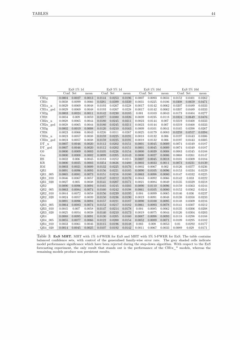
TABLES 44
ExS 1% 1d ExS 5% 1d ExS 1% 10d ExS 5% 10dConf. Set mean Conf. Set mean Conf. Set mean Conf. Set mean
CH1g 0.0004 0.0027 0.0013 0.0144 0.0253 0.0196 0.0007 0.0093 0.0034 0.0152 0.0401 0.0262CH1t 0.0038 0.0099 0.0066 0.0281 0.0399 0.0339 0.0031 0.0225 0.0106 0.0308 0.0659 0.0471CH1x_n 0.0029 0.0069 0.0048 0.0193 0.0267 0.0228 0.0017 0.0142 0.0062 0.0207 0.0489 0.0333CH1x_ged 0.0029 0.0069 0.0048 0.0193 0.0267 0.0228 0.0017 0.0142 0.0062 0.0207 0.0489 0.0333CH2g 0.0003 0.0024 0.0011 0.0142 0.0230 0.0185 0.001 0.0103 0.0043 0.0173 0.0404 0.0277CH2t 0.0034 0.009 0.0059 0.0277 0.0380 0.0326 0.0039 0.0235 0.0118 0.0324 0.0649 0.0476CH2x_n 0.0028 0.0065 0.0044 0.0180 0.0245 0.0211 0.0023 0.0144 0.007 0.0219 0.0468 0.0333CH2x_ged 0.0028 0.0065 0.0044 0.0180 0.0245 0.0211 0.0023 0.0144 0.007 0.0219 0.0468 0.0333CH3g 0.0002 0.0019 0.0008 0.0120 0.0210 0.0163 0.0009 0.0101 0.0041 0.0165 0.0398 0.0267CH3t 0.0023 0.0066 0.0043 0.0226 0.0311 0.0267 0.0025 0.0179 0.0083 0.0259 0.0557 0.0394CH3x_n 0.0023 0.0057 0.0038 0.0159 0.0225 0.0191 0.0018 0.0132 0.006 0.0197 0.0443 0.0306CH3x_ged 0.0023 0.0057 0.0038 0.0159 0.0225 0.0191 0.0018 0.0132 0.006 0.0197 0.0443 0.0305DT_n 0.0007 0.0046 0.0020 0.0112 0.0202 0.0151 0.0001 0.0045 0.0009 0.0074 0.0349 0.0187DT_ged 0.0007 0.0046 0.0020 0.0112 0.0202 0.0151 0.0001 0.0045 0.0009 0.0074 0.0349 0.0187G0 0.0000 0.0009 0.0003 0.0105 0.0226 0.0154 0.0000 0.0039 0.0008 0.0083 0.0345 0.0188Gm 0.0000 0.0008 0.0002 0.0099 0.0205 0.0143 0.0000 0.0027 0.0006 0.0068 0.0261 0.0147HS 0.0032 0.006 0.0045 0.0183 0.0252 0.0215 0.0007 0.0045 0.0018 0.0101 0.0309 0.0184KR 0.0000 0.0025 0.0003 0.0354 0.0626 0.0480 0.0002 0.0033 0.0011 0.0073 0.0231 0.0139RM 0.0003 0.0021 0.0009 0.0132 0.0225 0.0176 0.0002 0.0067 0.002 0.0126 0.0377 0.0236QR1 0.0091 0.0096 0.0093 0.0156 0.0221 0.0185 0.0090 0.0105 0.0096 0.0153 0.0334 0.0229QR1_005 0.0065 0.0081 0.0073 0.0151 0.0216 0.0180 0.0063 0.0098 0.0080 0.0147 0.0332 0.0225QR1_010 0.0046 0.0067 0.0057 0.0147 0.0212 0.0176 0.0043 0.0092 0.0066 0.0142 0.033 0.0222QR1_020 0.0027 0.005 0.0038 0.0141 0.0207 0.0171 0.0021 0.0084 0.0049 0.0135 0.0329 0.0218QR2 0.0090 0.0096 0.0094 0.0165 0.0245 0.0203 0.0090 0.0110 0.0096 0.0159 0.0363 0.0244QR2_005 0.0063 0.0084 0.0074 0.0160 0.0242 0.0198 0.0061 0.0105 0.0080 0.0152 0.0362 0.0241QR2_010 0.0044 0.0072 0.0058 0.0156 0.0239 0.0195 0.004 0.0099 0.0065 0.0146 0.036 0.0237QR2_020 0.0024 0.0057 0.0039 0.0150 0.0236 0.0190 0.0019 0.0091 0.0048 0.0138 0.0358 0.0233QR3 0.0091 0.0096 0.0094 0.0157 0.0221 0.0187 0.0090 0.0100 0.0095 0.0148 0.0309 0.0216QR3_005 0.0064 0.0083 0.0074 0.0152 0.0217 0.0182 0.0061 0.0093 0.0078 0.0141 0.0307 0.0212QR3_010 0.0045 0.007 0.0058 0.0147 0.0214 0.0178 0.004 0.0085 0.0062 0.0135 0.0306 0.0208QR3_020 0.0025 0.0054 0.0038 0.0140 0.0210 0.0173 0.0019 0.0075 0.0044 0.0126 0.0304 0.0203QR4 0.0088 0.0095 0.0091 0.0130 0.0205 0.0160 0.0087 0.0098 0.0093 0.0118 0.0298 0.0188QR4_005 0.0055 0.0077 0.0066 0.0122 0.0200 0.0154 0.0052 0.0089 0.0071 0.0109 0.0295 0.0182QR4_010 0.0033 0.0061 0.0046 0.0115 0.0196 0.0148 0.003 0.008 0.0053 0.01 0.0292 0.0177QR4_020 0.0014 0.0045 0.0025 0.0107 0.0192 0.0142 0.0011 0.0067 0.0033 0.0089 0.029 0.0171
Table 3: ExS MHT. MHT with 1% 4-FWER for ExS and MHT with 5% 5-FWER for ExS. The table containsbalanced confidence sets, with control of the generalised family-wise error rate. The grey shaded cells indicatemodel performance significance which have been rejected during the step-down algorithm. With respect to the ExSforecasting experiment, the only result that stands out is the performance of the CH1x_* models, whereas theremaining models produce non persistent results.

45 CHAPTER 2. MODEL SELECTION OF MARKET RISK MODELS
VaR 1% 1d VaR 5% 1d VaR 1% 10d VaR 5% 10dConf. Set mean Conf. Set mean Conf. Set mean Conf. Set mean
CH1g 0.0041 0.0215 0.0120 0.0180 0.0479 0.0317 0.0000 0.0119 0.0030 0.0053 0.0481 0.0227CH1t 0.0000 0.0101 0.0039 0.0094 0.0345 0.0210 0.0000 0.0081 0.0008 0.0005 0.0303 0.0118CH1x_n 0.0004 0.0132 0.0060 0.0197 0.0490 0.0335 0.0000 0.0105 0.0016 0.0029 0.0400 0.0178CH1x_ged 0.0004 0.0132 0.0060 0.0197 0.0490 0.0335 0.0000 0.0105 0.0016 0.0029 0.0400 0.0178CH2g 0.0042 0.0202 0.0117 0.0177 0.0446 0.0308 0.0000 0.0114 0.0021 0.0046 0.0420 0.0201CH2t 0.0000 0.0107 0.0044 0.0114 0.0346 0.0223 0.0000 0.0071 0.0006 0.0003 0.0280 0.0111CH2x_n 0.0007 0.0130 0.0060 0.0199 0.0471 0.0334 0.0000 0.0084 0.0011 0.0025 0.0359 0.0161CH2x_ged 0.0007 0.0130 0.0060 0.0199 0.0471 0.0334 0.0000 0.0084 0.0011 0.0025 0.0359 0.0161CH3g 0.0054 0.0225 0.0132 0.0202 0.0498 0.0334 0.0000 0.0112 0.0029 0.0053 0.0449 0.0219CH3t 0.0011 0.0148 0.0067 0.0154 0.0410 0.0270 0.0000 0.0101 0.0015 0.0025 0.0359 0.0159CH3x_n 0.0017 0.0156 0.0076 0.0250 0.0510 0.0375 0.0000 0.0113 0.0020 0.0039 0.0413 0.0192CH3x_ged 0.0017 0.0156 0.0076 0.0250 0.0510 0.0375 0.0000 0.0113 0.0020 0.0039 0.0413 0.0192CH1g_avg - - - - - - 0.0000 0.0032 0.0001 0.0000 0.0190 0.0053CH1t_avg - - - - - - 0.0000 0.0000 0.0000 0.0000 0.0088 0.0014CH1x_n_avg - - - - - - 0.0000 0.0011 0.0000 0.0000 0.0135 0.0030CH1x_ged_avg - - - - - - 0.0000 0.0011 0.0000 0.0000 0.0135 0.0030CH2g_avg - - - - - - 0.0000 0.0017 0.0000 0.0000 0.0170 0.0046CH2t_avg - - - - - - 0.0000 0.0000 0.0000 0.0000 0.0084 0.0012CH2x_n_avg - - - - - - 0.0000 0.0004 0.0000 0.0000 0.0125 0.0026CH2x_ged_avg - - - - - - 0.0000 0.0004 0.0000 0.0000 0.0125 0.0026CH3g_avg - - - - - - 0.0000 0.0016 0.0000 0.0000 0.0149 0.0036CH3t_avg - - - - - - 0.0000 0.0000 0.0000 0.0000 0.0088 0.0014CH3x_n_avg - - - - - - 0.0000 0.0008 0.0000 0.0000 0.0127 0.0027CH3x_ged_avg - - - - - - 0.0000 0.0008 0.0000 0.0000 0.0127 0.0027DT_n 0.0000 0.0047 0.0010 0.0019 0.0215 0.0104 0.0000 0.0032 0.0001 0.0000 0.0095 0.0016DT_ged 0.0000 0.0047 0.0010 0.0019 0.0215 0.0104 0.0000 0.0032 0.0001 0.0000 0.0095 0.0016G0 0.0014 0.0181 0.0081 0.0115 0.0403 0.0256 0.0000 0.0163 0.0044 0.0022 0.0442 0.0191Gm 0.0015 0.0181 0.0084 0.0126 0.0426 0.0274 0.0004 0.0196 0.0064 0.0066 0.0531 0.0261HS 0.0012 0.0127 0.0065 0.0128 0.0409 0.0267 0.0000 0.0173 0.0056 0.0056 0.0496 0.0242KR 0.0000 0.0047 0.0010 0.0000 0.0044 0.0010 0.0000 0.0044 0.0002 0.0000 0.0223 0.0079RM 0.0066 0.0263 0.0158 0.0348 0.0649 0.0491 0.0026 0.0259 0.0103 0.0162 0.0656 0.0386QR1 0.0039 0.0185 0.0103 0.0506 0.0825 0.0654 0.0008 0.0199 0.0066 0.0275 0.0779 0.0508QR2 0.0012 0.0163 0.0079 0.0183 0.0496 0.0335 0.0000 0.0125 0.0032 0.0073 0.0560 0.0273QR3 0.0010 0.0141 0.0066 0.0218 0.0518 0.0356 0.0000 0.0122 0.0025 0.0127 0.0517 0.0306QR4 0.0000 0.0056 0.0013 0.0096 0.0363 0.0224 0.0000 0.0057 0.0003 0.0022 0.0393 0.0169
Table 4: L/V VaR MHT. L/V MHT with 1% 3-FWER for ECP and L/V MHT with 5% 4-FWER for ECP. Thetable contains balanced confidence sets, with control of the generalised family-wise error rate. The grey shaded cellsindicate model performance significance which have been rejected during the step-down algorithm. The low volatilityscenario is the only environment where the CH1x_* models do not produce significant performances, whereas theonly model that performs well under this volatility condition is the RM.
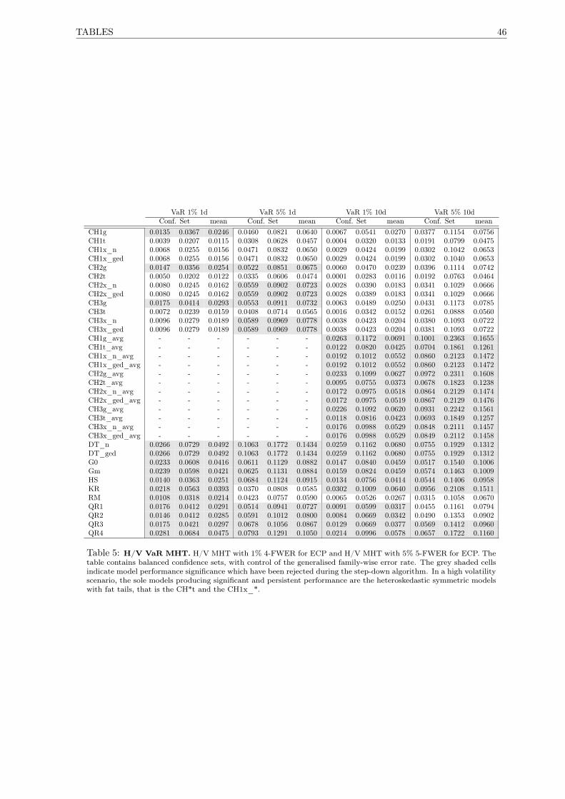
TABLES 46
VaR 1% 1d VaR 5% 1d VaR 1% 10d VaR 5% 10dConf. Set mean Conf. Set mean Conf. Set mean Conf. Set mean
CH1g 0.0135 0.0367 0.0246 0.0460 0.0821 0.0640 0.0067 0.0541 0.0270 0.0377 0.1154 0.0756CH1t 0.0039 0.0207 0.0115 0.0308 0.0628 0.0457 0.0004 0.0320 0.0133 0.0191 0.0799 0.0475CH1x_n 0.0068 0.0255 0.0156 0.0471 0.0832 0.0650 0.0029 0.0424 0.0199 0.0302 0.1042 0.0653CH1x_ged 0.0068 0.0255 0.0156 0.0471 0.0832 0.0650 0.0029 0.0424 0.0199 0.0302 0.1040 0.0653CH2g 0.0147 0.0356 0.0254 0.0522 0.0851 0.0675 0.0060 0.0470 0.0239 0.0396 0.1114 0.0742CH2t 0.0050 0.0202 0.0122 0.0335 0.0606 0.0474 0.0001 0.0283 0.0116 0.0192 0.0763 0.0464CH2x_n 0.0080 0.0245 0.0162 0.0559 0.0902 0.0723 0.0028 0.0390 0.0183 0.0341 0.1029 0.0666CH2x_ged 0.0080 0.0245 0.0162 0.0559 0.0902 0.0723 0.0028 0.0389 0.0183 0.0341 0.1029 0.0666CH3g 0.0175 0.0414 0.0293 0.0553 0.0911 0.0732 0.0063 0.0489 0.0250 0.0431 0.1173 0.0785CH3t 0.0072 0.0239 0.0159 0.0408 0.0714 0.0565 0.0016 0.0342 0.0152 0.0261 0.0888 0.0560CH3x_n 0.0096 0.0279 0.0189 0.0589 0.0969 0.0778 0.0038 0.0423 0.0204 0.0380 0.1093 0.0722CH3x_ged 0.0096 0.0279 0.0189 0.0589 0.0969 0.0778 0.0038 0.0423 0.0204 0.0381 0.1093 0.0722CH1g_avg - - - - - - 0.0263 0.1172 0.0691 0.1001 0.2363 0.1655CH1t_avg - - - - - - 0.0122 0.0820 0.0425 0.0704 0.1861 0.1261CH1x_n_avg - - - - - - 0.0192 0.1012 0.0552 0.0860 0.2123 0.1472CH1x_ged_avg - - - - - - 0.0192 0.1012 0.0552 0.0860 0.2123 0.1472CH2g_avg - - - - - - 0.0233 0.1099 0.0627 0.0972 0.2311 0.1608CH2t_avg - - - - - - 0.0095 0.0755 0.0373 0.0678 0.1823 0.1238CH2x_n_avg - - - - - - 0.0172 0.0975 0.0518 0.0864 0.2129 0.1474CH2x_ged_avg - - - - - - 0.0172 0.0975 0.0519 0.0867 0.2129 0.1476CH3g_avg - - - - - - 0.0226 0.1092 0.0620 0.0931 0.2242 0.1561CH3t_avg - - - - - - 0.0118 0.0816 0.0423 0.0693 0.1849 0.1257CH3x_n_avg - - - - - - 0.0176 0.0988 0.0529 0.0848 0.2111 0.1457CH3x_ged_avg - - - - - - 0.0176 0.0988 0.0529 0.0849 0.2112 0.1458DT_n 0.0266 0.0729 0.0492 0.1063 0.1772 0.1434 0.0259 0.1162 0.0680 0.0755 0.1929 0.1312DT_ged 0.0266 0.0729 0.0492 0.1063 0.1772 0.1434 0.0259 0.1162 0.0680 0.0755 0.1929 0.1312G0 0.0233 0.0608 0.0416 0.0611 0.1129 0.0882 0.0147 0.0840 0.0459 0.0517 0.1540 0.1006Gm 0.0239 0.0598 0.0421 0.0625 0.1131 0.0884 0.0159 0.0824 0.0459 0.0574 0.1463 0.1009HS 0.0140 0.0363 0.0251 0.0684 0.1124 0.0915 0.0134 0.0756 0.0414 0.0544 0.1406 0.0958KR 0.0218 0.0563 0.0393 0.0370 0.0808 0.0585 0.0302 0.1009 0.0640 0.0956 0.2108 0.1511RM 0.0108 0.0318 0.0214 0.0423 0.0757 0.0590 0.0065 0.0526 0.0267 0.0315 0.1058 0.0670QR1 0.0176 0.0412 0.0291 0.0514 0.0941 0.0727 0.0091 0.0599 0.0317 0.0455 0.1161 0.0794QR2 0.0146 0.0412 0.0285 0.0591 0.1012 0.0800 0.0084 0.0669 0.0342 0.0490 0.1353 0.0902QR3 0.0175 0.0421 0.0297 0.0678 0.1056 0.0867 0.0129 0.0669 0.0377 0.0569 0.1412 0.0960QR4 0.0281 0.0684 0.0475 0.0793 0.1291 0.1050 0.0214 0.0996 0.0578 0.0657 0.1722 0.1160
Table 5: H/V VaR MHT. H/V MHT with 1% 4-FWER for ECP and H/V MHT with 5% 5-FWER for ECP. Thetable contains balanced confidence sets, with control of the generalised family-wise error rate. The grey shaded cellsindicate model performance significance which have been rejected during the step-down algorithm. In a high volatilityscenario, the sole models producing significant and persistent performance are the heteroskedastic symmetric modelswith fat tails, that is the CH*t and the CH1x_*.
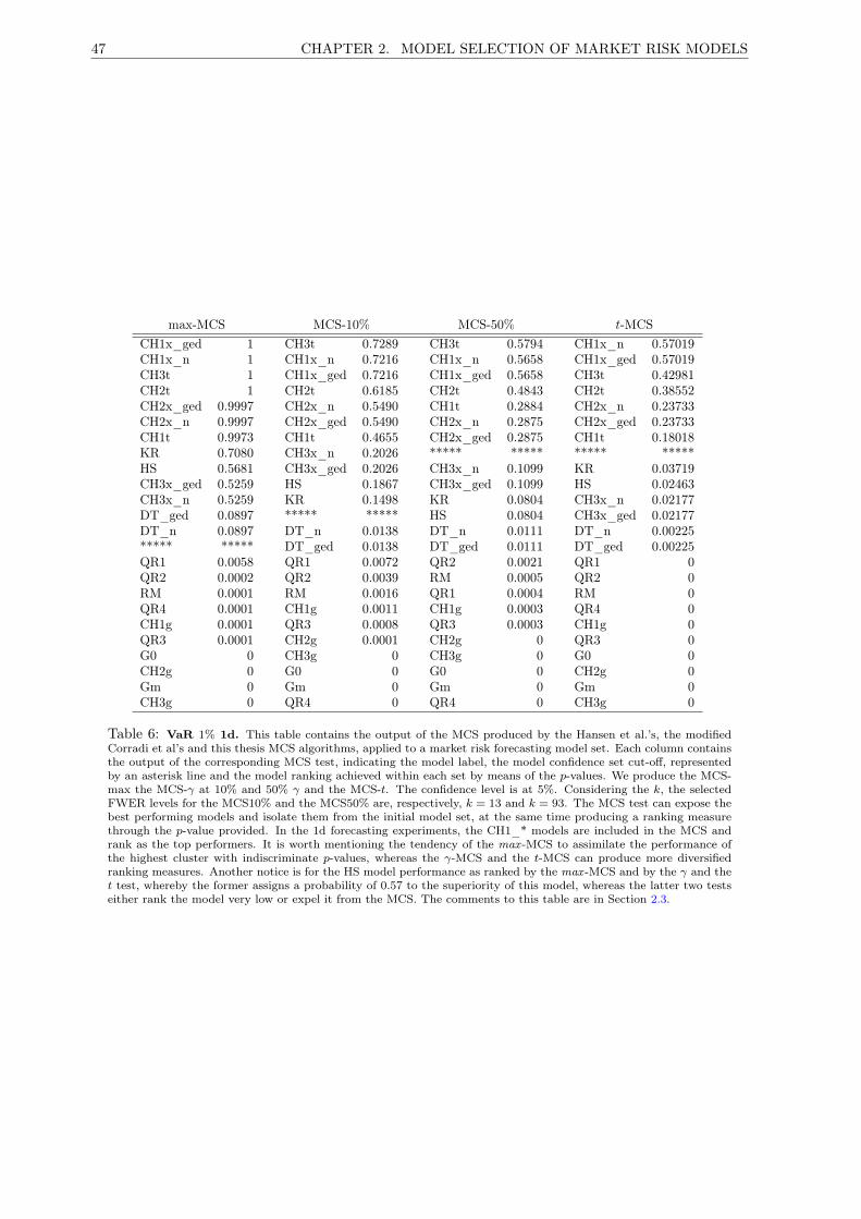
47 CHAPTER 2. MODEL SELECTION OF MARKET RISK MODELS
max-MCS MCS-10% MCS-50% t-MCSCH1x_ged 1 CH3t 0.7289 CH3t 0.5794 CH1x_n 0.57019CH1x_n 1 CH1x_n 0.7216 CH1x_n 0.5658 CH1x_ged 0.57019CH3t 1 CH1x_ged 0.7216 CH1x_ged 0.5658 CH3t 0.42981CH2t 1 CH2t 0.6185 CH2t 0.4843 CH2t 0.38552CH2x_ged 0.9997 CH2x_n 0.5490 CH1t 0.2884 CH2x_n 0.23733CH2x_n 0.9997 CH2x_ged 0.5490 CH2x_n 0.2875 CH2x_ged 0.23733CH1t 0.9973 CH1t 0.4655 CH2x_ged 0.2875 CH1t 0.18018KR 0.7080 CH3x_n 0.2026 ***** ***** ***** *****HS 0.5681 CH3x_ged 0.2026 CH3x_n 0.1099 KR 0.03719CH3x_ged 0.5259 HS 0.1867 CH3x_ged 0.1099 HS 0.02463CH3x_n 0.5259 KR 0.1498 KR 0.0804 CH3x_n 0.02177DT_ged 0.0897 ***** ***** HS 0.0804 CH3x_ged 0.02177DT_n 0.0897 DT_n 0.0138 DT_n 0.0111 DT_n 0.00225***** ***** DT_ged 0.0138 DT_ged 0.0111 DT_ged 0.00225QR1 0.0058 QR1 0.0072 QR2 0.0021 QR1 0QR2 0.0002 QR2 0.0039 RM 0.0005 QR2 0RM 0.0001 RM 0.0016 QR1 0.0004 RM 0QR4 0.0001 CH1g 0.0011 CH1g 0.0003 QR4 0CH1g 0.0001 QR3 0.0008 QR3 0.0003 CH1g 0QR3 0.0001 CH2g 0.0001 CH2g 0 QR3 0G0 0 CH3g 0 CH3g 0 G0 0CH2g 0 G0 0 G0 0 CH2g 0Gm 0 Gm 0 Gm 0 Gm 0CH3g 0 QR4 0 QR4 0 CH3g 0
Table 6: VaR 1% 1d. This table contains the output of the MCS produced by the Hansen et al.’s, the modifiedCorradi et al’s and this thesis MCS algorithms, applied to a market risk forecasting model set. Each column containsthe output of the corresponding MCS test, indicating the model label, the model confidence set cut-off, representedby an asterisk line and the model ranking achieved within each set by means of the p-values. We produce the MCS-max the MCS-γ at 10% and 50% γ and the MCS-t. The confidence level is at 5%. Considering the k, the selectedFWER levels for the MCS10% and the MCS50% are, respectively, k = 13 and k = 93. The MCS test can expose thebest performing models and isolate them from the initial model set, at the same time producing a ranking measurethrough the p-value provided. In the 1d forecasting experiments, the CH1_* models are included in the MCS andrank as the top performers. It is worth mentioning the tendency of the max -MCS to assimilate the performance ofthe highest cluster with indiscriminate p-values, whereas the γ-MCS and the t-MCS can produce more diversifiedranking measures. Another notice is for the HS model performance as ranked by the max -MCS and by the γ and thet test, whereby the former assigns a probability of 0.57 to the superiority of this model, whereas the latter two testseither rank the model very low or expel it from the MCS. The comments to this table are in Section 2.3.

TABLES 48
max-MCS MCS-10% MCS-50% t-MCSCH1g 1 CH1g 0.8453 CH1g 0.7924 CH1g 0.68824CH2g 0.9999 CH2g 0.7276 CH2g 0.6023 CH2g 0.31176CH1x_ged 0.9998 CH1x_n 0.7013 CH1x_n 0.5716 CH1x_n 0.26866CH1x_n 0.9998 CH1x_ged 0.7013 CH1x_ged 0.5716 CH1x_ged 0.26866CH3t 0.9996 G0 0.6085 G0 0.4991 CH3t 0.23502G0 0.9995 RM 0.5240 CH3t 0.4019 G0 0.23264RM 0.9877 CH3t 0.4920 RM 0.3598 RM 0.14665Gm 0.9623 Gm 0.3941 Gm 0.2503 Gm 0.10926HS 0.9385 HS 0.3478 HS 0.2009 HS 0.09201CH3g 0.5527 CH3g 0.3260 ***** ***** ***** *****CH2x_ged 0.1291 CH2x_n 0.2448 CH3g 0.2047 CH3g 0.02346CH2x_n 0.1291 CH2x_ged 0.2448 CH2x_n 0.1749 CH2x_n 0.00322***** ***** QR2 0.033 CH2x_ged 0.1749 CH2x_ged 0.00322QR2 0.0306 ***** ***** CH2t 0.0482 QR2 0.00050QR1 0.0306 CH2t 0.0911 QR2 0.0375 QR1 0.00042CH3x_ged 0.0008 CH1t 0.0607 CH1t 0.0324 CH3x_n 0CH3x_n 0.0008 CH3x_n 0.0460 CH3x_n 0.0253 CH3x_ged 0CH2t 0.0002 CH3x_ged 0.0460 CH3x_ged 0.0253 CH2t 0QR4 0.0001 QR1 0.0232 QR1 0.0071 QR4 0DT_ged 0.0001 QR4 0.0013 QR4 0.0018 DT_n 0DT_n 0.0001 QR3 0.0012 QR3 0.0012 DT_ged 0CH1t 0.0001 DT_n 0.0003 DT_n 0.0004 CH1t 0QR3 0 DT_ged 0.0003 DT_ged 0.0004 QR3 0KR 0 KR 0 KR 0 KR 0
Table 7: VaR 5% 1d. This table contains the output of the MCS produced by the Hansen et al.’s, the modifiedCorradi et al’s and this thesis MCS algorithms, applied to a market risk forecasting model set. Each column containsthe output of the corresponding MCS test, indicating the model label, the model confidence set cut-off, represented byan asterisk line and the model ranking achieved within each set by means of the p-values. We produce the MCS-maxthe MCS-γ at 10% and 50% γ and the MCS-t. The confidence level is at 5%. Considering the k, the selected FWERlevels for the MCS10% and the MCS50% are, respectively, k = 10 and k = 67. In this experiment, the heteroskedasticmodels perform best again, with EVD extension as well as the Gaussian type. Some practitioner models such as G0and RM also enter the MCS. Although both tests produce the same MCS, the contrast between the max -MCS andthe MHT based MCS can be seen from the p-value measure, whereby, for instance, the HS model is ranked at 0.94 inthe former and 0.35 in the latter. The comments to this table are in Section 2.3.
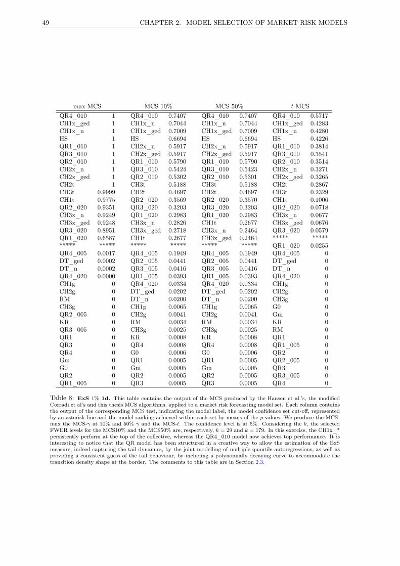
49 CHAPTER 2. MODEL SELECTION OF MARKET RISK MODELS
max-MCS MCS-10% MCS-50% t-MCSQR4_010 1 QR4_010 0.7407 QR4_010 0.7407 QR4_010 0.5717CH1x_ged 1 CH1x_n 0.7044 CH1x_n 0.7044 CH1x_ged 0.4283CH1x_n 1 CH1x_ged 0.7009 CH1x_ged 0.7009 CH1x_n 0.4280HS 1 HS 0.6694 HS 0.6694 HS 0.4226QR1_010 1 CH2x_n 0.5917 CH2x_n 0.5917 QR1_010 0.3814QR3_010 1 CH2x_ged 0.5917 CH2x_ged 0.5917 QR3_010 0.3541QR2_010 1 QR1_010 0.5790 QR1_010 0.5790 QR2_010 0.3514CH2x_n 1 QR3_010 0.5424 QR3_010 0.5423 CH2x_n 0.3271CH2x_ged 1 QR2_010 0.5302 QR2_010 0.5301 CH2x_ged 0.3265CH2t 1 CH3t 0.5188 CH3t 0.5188 CH2t 0.2867CH3t 0.9999 CH2t 0.4697 CH2t 0.4697 CH3t 0.2329CH1t 0.9775 QR2_020 0.3569 QR2_020 0.3570 CH1t 0.1006QR2_020 0.9351 QR3_020 0.3203 QR3_020 0.3203 QR2_020 0.0718CH3x_n 0.9249 QR1_020 0.2983 QR1_020 0.2983 CH3x_n 0.0677CH3x_ged 0.9248 CH3x_n 0.2826 CH1t 0.2677 CH3x_ged 0.0676QR3_020 0.8951 CH3x_ged 0.2718 CH3x_n 0.2464 QR3_020 0.0579QR1_020 0.6587 CH1t 0.2677 CH3x_ged 0.2464 ***** ********** ***** ***** ***** ***** ***** QR1_020 0.0255QR4_005 0.0017 QR4_005 0.1949 QR4_005 0.1949 QR4_005 0DT_ged 0.0002 QR2_005 0.0441 QR2_005 0.0441 DT_ged 0DT_n 0.0002 QR3_005 0.0416 QR3_005 0.0416 DT_n 0QR4_020 0.0000 QR1_005 0.0393 QR1_005 0.0393 QR4_020 0CH1g 0 QR4_020 0.0334 QR4_020 0.0334 CH1g 0CH2g 0 DT_ged 0.0202 DT_ged 0.0202 CH2g 0RM 0 DT_n 0.0200 DT_n 0.0200 CH3g 0CH3g 0 CH1g 0.0065 CH1g 0.0065 G0 0QR2_005 0 CH2g 0.0041 CH2g 0.0041 Gm 0KR 0 RM 0.0034 RM 0.0034 KR 0QR3_005 0 CH3g 0.0025 CH3g 0.0025 RM 0QR1 0 KR 0.0008 KR 0.0008 QR1 0QR3 0 QR4 0.0008 QR4 0.0008 QR1_005 0QR4 0 G0 0.0006 G0 0.0006 QR2 0Gm 0 QR1 0.0005 QR1 0.0005 QR2_005 0G0 0 Gm 0.0005 Gm 0.0005 QR3 0QR2 0 QR2 0.0005 QR2 0.0005 QR3_005 0QR1_005 0 QR3 0.0005 QR3 0.0005 QR4 0
Table 8: ExS 1% 1d. This table contains the output of the MCS produced by the Hansen et al.’s, the modifiedCorradi et al’s and this thesis MCS algorithms, applied to a market risk forecasting model set. Each column containsthe output of the corresponding MCS test, indicating the model label, the model confidence set cut-off, representedby an asterisk line and the model ranking achieved within each set by means of the p-values. We produce the MCS-max the MCS-γ at 10% and 50% γ and the MCS-t. The confidence level is at 5%. Considering the k, the selectedFWER levels for the MCS10% and the MCS50% are, respectively, k = 29 and k = 179. In this exercise, the CH1x_*persistently perform at the top of the collective, whereas the QR4_010 model now achieves top performance. It isinteresting to notice that the QR model has been structured in a creative way to allow the estimation of the ExSmeasure, indeed capturing the tail dynamics, by the joint modelling of multiple quantile autoregressions, as well asproviding a consistent guess of the tail behaviour, by including a polynomially decaying curve to accommodate thetransition density shape at the border. The comments to this table are in Section 2.3.
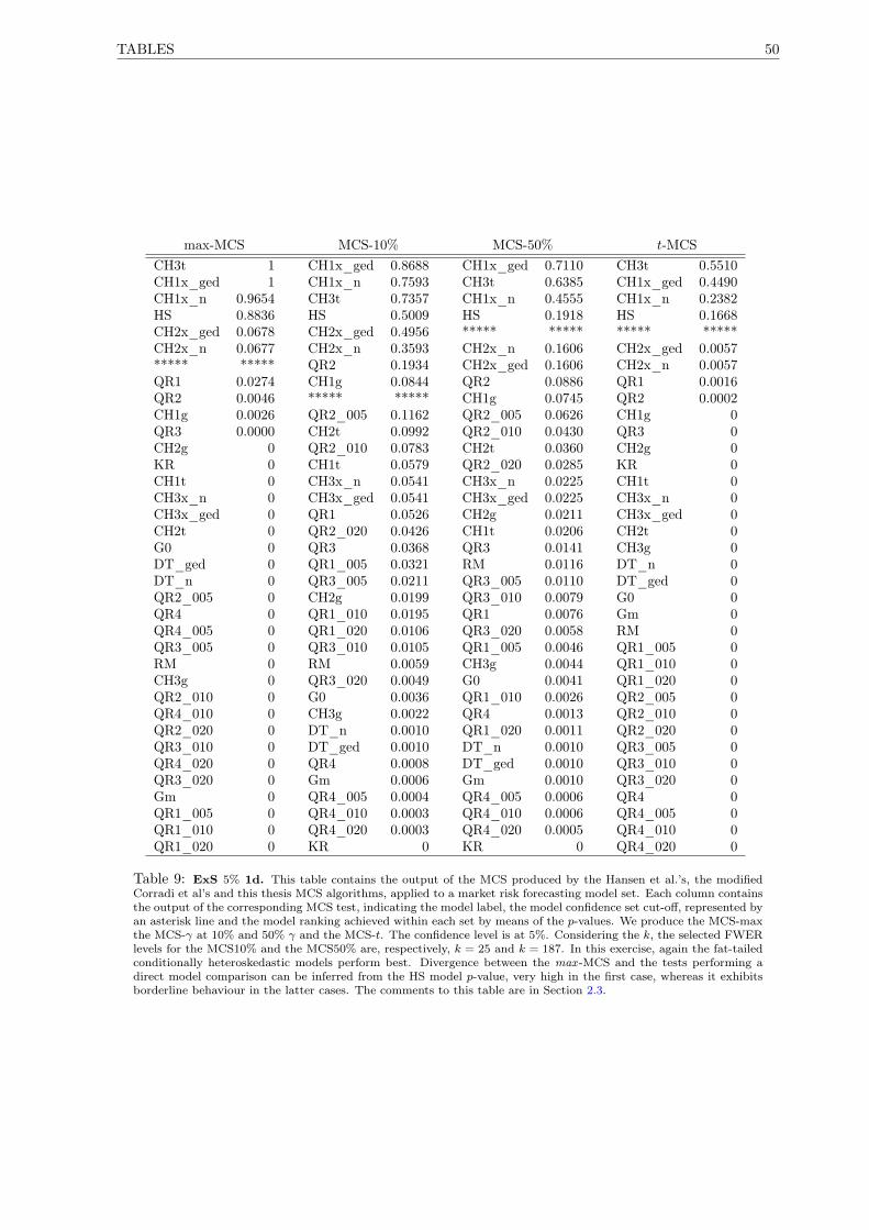
TABLES 50
max-MCS MCS-10% MCS-50% t-MCSCH3t 1 CH1x_ged 0.8688 CH1x_ged 0.7110 CH3t 0.5510CH1x_ged 1 CH1x_n 0.7593 CH3t 0.6385 CH1x_ged 0.4490CH1x_n 0.9654 CH3t 0.7357 CH1x_n 0.4555 CH1x_n 0.2382HS 0.8836 HS 0.5009 HS 0.1918 HS 0.1668CH2x_ged 0.0678 CH2x_ged 0.4956 ***** ***** ***** *****CH2x_n 0.0677 CH2x_n 0.3593 CH2x_n 0.1606 CH2x_ged 0.0057***** ***** QR2 0.1934 CH2x_ged 0.1606 CH2x_n 0.0057QR1 0.0274 CH1g 0.0844 QR2 0.0886 QR1 0.0016QR2 0.0046 ***** ***** CH1g 0.0745 QR2 0.0002CH1g 0.0026 QR2_005 0.1162 QR2_005 0.0626 CH1g 0QR3 0.0000 CH2t 0.0992 QR2_010 0.0430 QR3 0CH2g 0 QR2_010 0.0783 CH2t 0.0360 CH2g 0KR 0 CH1t 0.0579 QR2_020 0.0285 KR 0CH1t 0 CH3x_n 0.0541 CH3x_n 0.0225 CH1t 0CH3x_n 0 CH3x_ged 0.0541 CH3x_ged 0.0225 CH3x_n 0CH3x_ged 0 QR1 0.0526 CH2g 0.0211 CH3x_ged 0CH2t 0 QR2_020 0.0426 CH1t 0.0206 CH2t 0G0 0 QR3 0.0368 QR3 0.0141 CH3g 0DT_ged 0 QR1_005 0.0321 RM 0.0116 DT_n 0DT_n 0 QR3_005 0.0211 QR3_005 0.0110 DT_ged 0QR2_005 0 CH2g 0.0199 QR3_010 0.0079 G0 0QR4 0 QR1_010 0.0195 QR1 0.0076 Gm 0QR4_005 0 QR1_020 0.0106 QR3_020 0.0058 RM 0QR3_005 0 QR3_010 0.0105 QR1_005 0.0046 QR1_005 0RM 0 RM 0.0059 CH3g 0.0044 QR1_010 0CH3g 0 QR3_020 0.0049 G0 0.0041 QR1_020 0QR2_010 0 G0 0.0036 QR1_010 0.0026 QR2_005 0QR4_010 0 CH3g 0.0022 QR4 0.0013 QR2_010 0QR2_020 0 DT_n 0.0010 QR1_020 0.0011 QR2_020 0QR3_010 0 DT_ged 0.0010 DT_n 0.0010 QR3_005 0QR4_020 0 QR4 0.0008 DT_ged 0.0010 QR3_010 0QR3_020 0 Gm 0.0006 Gm 0.0010 QR3_020 0Gm 0 QR4_005 0.0004 QR4_005 0.0006 QR4 0QR1_005 0 QR4_010 0.0003 QR4_010 0.0006 QR4_005 0QR1_010 0 QR4_020 0.0003 QR4_020 0.0005 QR4_010 0QR1_020 0 KR 0 KR 0 QR4_020 0
Table 9: ExS 5% 1d. This table contains the output of the MCS produced by the Hansen et al.’s, the modifiedCorradi et al’s and this thesis MCS algorithms, applied to a market risk forecasting model set. Each column containsthe output of the corresponding MCS test, indicating the model label, the model confidence set cut-off, represented byan asterisk line and the model ranking achieved within each set by means of the p-values. We produce the MCS-maxthe MCS-γ at 10% and 50% γ and the MCS-t. The confidence level is at 5%. Considering the k, the selected FWERlevels for the MCS10% and the MCS50% are, respectively, k = 25 and k = 187. In this exercise, again the fat-tailedconditionally heteroskedastic models perform best. Divergence between the max -MCS and the tests performing adirect model comparison can be inferred from the HS model p-value, very high in the first case, whereas it exhibitsborderline behaviour in the latter cases. The comments to this table are in Section 2.3.

51 CHAPTER 2. MODEL SELECTION OF MARKET RISK MODELS
max-MCS MCS-10% MCS-50% t-MCSCH3x_ged 1 CH2g 0.7743 CH2g 0.7743 CH3x_ged 0.5065CH3x_n 1 CH3g 0.7648 CH3g 0.7648 CH3x_n 0.4935CH2g 1 CH3x_ged 0.7344 CH3x_ged 0.7344 CH2g 0.4789CH3g 1 CH3x_n 0.7339 CH3x_n 0.7339 CH3g 0.4367CH1x_n 1 CH2t_avg 0.7288 CH2t_avg 0.7288 CH1x_n 0.4340CH1x_ged 1 CH1g 0.7215 CH1g 0.7215 CH1x_ged 0.4337CH2t_avg 1 CH1x_n 0.7094 CH1x_n 0.7094 CH2t_avg 0.4142CH2x_n 1 CH1x_ged 0.7094 CH1x_ged 0.7094 CH2x_n 0.3747CH2x_ged 1 CH1t_avg 0.6987 CH1t_avg 0.6987 CH2x_ged 0.3738CH1t_avg 1 CH3t_avg 0.6952 CH3t_avg 0.6952 CH1t_avg 0.3280CH3t_avg 1 CH2x_n 0.6684 CH2x_n 0.6684 CH3t_avg 0.3253CH1g 1 CH2x_ged 0.6680 CH2x_ged 0.6680 CH1g 0.3060CH3t 1 CH3t 0.5921 CH3t 0.5921 CH3t 0.2438QR1 1 QR1 0.5820 QR1 0.5820 QR1 0.1959QR2 1 QR2 0.5748 QR2 0.5748 QR2 0.1442CH2x_n_avg 1 CH2x_n_avg 0.5610 CH2x_n_avg 0.5610 CH2x_n_avg 0.1422CH2x_ged_avg 1 CH2x_ged_avg 0.5585 CH2x_ged_avg 0.5585 CH2x_ged_avg 0.1416RM 1 RM 0.5510 RM 0.5510 RM 0.1394CH3x_n_avg 1 CH1t 0.5061 CH1t 0.5061 CH3x_n_avg 0.1237CH3x_ged_avg 1 CH3x_n_avg 0.4999 CH3x_n_avg 0.4999 CH3x_ged_avg 0.1230CH1t 1 CH3x_ged_avg 0.4969 CH3x_ged_avg 0.4969 CH1t 0.1146CH1x_ged_avg 0.9994 CH2t 0.4539 CH2t 0.4539 CH1x_ged_avg 0.0863CH1x_n_avg 0.9994 CH1x_ged_avg 0.4256 CH1x_ged_avg 0.4256 CH1x_n_avg 0.0862QR3 0.9975 CH1x_n_avg 0.4247 CH1x_n_avg 0.4247 QR3 0.0699CH2t 0.9966 QR3 0.4243 QR3 0.4243 CH2t 0.0668G0 0.9553 CH3g_avg 0.3025 CH3g_avg 0.3025 ***** *****QR4 0.9032 CH2g_avg 0.2760 CH2g_avg 0.2760 G0 0.0346HS 0.8923 HS 0.2409 HS 0.2409 QR4 0.0248CH3g_avg 0.8873 G0 0.2259 G0 0.2259 HS 0.0235CH2g_avg 0.8480 QR4 0.1881 QR4 0.1881 CH3g_avg 0.0229KR 0.7021 DT_ged 0.1494 DT_ged 0.1494 CH2g_avg 0.0194DT_ged 0.5064 DT_n 0.1485 DT_n 0.1485 KR 0.0118DT_n 0.5051 KR 0.1277 KR 0.1277 DT_ged 0.0063CH1g_avg 0.4029 CH1g_avg 0.1092 CH1g_avg 0.1092 DT_n 0.0062Gm 0.3389 Gm 0.0739 Gm 0.0739 CH1g_avg 0.0044***** ***** ***** ***** ***** ***** Gm 0.0034
Table 10: VaR 1% 2w. This table contains the output of the MCS produced by the Hansen et al.’s, the modifiedCorradi et al’s and this thesis MCS algorithms, applied to a market risk forecasting model set. Each column containsthe output of the corresponding MCS test, indicating the model label, the model confidence set cut-off, represented byan asterisk line and the model ranking achieved within each set by means of the p-values. We produce the MCS-maxthe MCS-γ at 10% and 50% γ and the MCS-t. The confidence level is at 5%. Considering the k, the selected FWERlevels for the MCS10% and the MCS50% are, respectively, k = 1 and k = 1. In the 2w forecasting experiments, themodel performances are more widespread. The top models CH1x_* either rank at the top of the MCS or are thereincluded. The comments to this table are in Section 2.3.

TABLES 52
max-MCS MCS-10% MCS-50% t-MCSRM 1 G0 0.6894 G0 0.6894 RM 0.5025G0 1 QR1 0.6783 QR1 0.6783 G0 0.4975QR1 1 RM 0.6753 RM 0.6753 QR1 0.4962DT_n 1 CH3g 0.6619 CH3g 0.6619 DT_n 0.4746DT_ged 1 DT_n 0.6596 DT_n 0.6596 DT_ged 0.4743CH3g 1 DT_ged 0.6591 DT_ged 0.6591 CH3g 0.4736CH1t_avg 1 QR2 0.6573 QR2 0.6573 CH1t_avg 0.4702CH3t_avg 1 HS 0.6565 HS 0.6565 CH3t_avg 0.4675HS 1 CH1t_avg 0.6530 CH1t_avg 0.6530 HS 0.4330QR2 1 CH3t_avg 0.6487 CH3t_avg 0.6487 QR2 0.4288CH2t_avg 1 CH1g 0.6332 CH1g 0.6332 CH2t_avg 0.4284CH1g 1 CH2t_avg 0.6281 CH2t_avg 0.6281 CH1g 0.3863CH2g 1 CH2g 0.6039 CH2g 0.6039 CH2g 0.3278CH3x_n_avg 1 CH3x_n_avg 0.5311 CH3x_n_avg 0.5311 CH3x_n_avg 0.2573CH3x_ged_avg 1 CH3x_ged_avg 0.5252 CH3x_ged_avg 0.5252 CH3x_ged_avg 0.2557CH2x_n_avg 1 Gm 0.5126 Gm 0.5126 CH2x_n_avg 0.2320CH2x_ged_avg 1 CH3x_ged 0.4990 CH3x_ged 0.4990 CH2x_ged_avg 0.2188CH1x_ged_avg 1 CH3x_n 0.4939 CH3x_n 0.4939 CH1x_ged_avg 0.1938CH1x_n_avg 1 CH2x_n_avg 0.4667 CH2x_n_avg 0.4667 CH1x_n_avg 0.1906CH3x_ged 1 QR3 0.4567 QR3 0.4567 CH3x_ged 0.1865CH3x_n 1 CH2x_ged_avg 0.4544 CH2x_ged_avg 0.4544 CH3x_n 0.1857QR3 1 CH1x_ged_avg 0.4412 CH1x_ged_avg 0.4412 QR3 0.1831QR4 1 CH1x_n_avg 0.4352 CH1x_n_avg 0.4352 QR4 0.1750Gm 1 QR4 0.4242 QR4 0.4242 Gm 0.1676CH3g_avg 0.9940 CH2x_n 0.3532 CH2x_n 0.3532 CH3g_avg 0.0696CH2x_n 0.9932 CH2x_ged 0.3513 CH2x_ged 0.3513 CH2x_n 0.0677CH2x_ged 0.9929 CH1x_n 0.3239 CH1x_n 0.3239 CH2x_ged 0.0672KR 0.9901 CH1x_ged 0.3203 CH1x_ged 0.3203 KR 0.0620CH1x_n 0.9875 CH3g_avg 0.3065 CH3g_avg 0.3065 CH1x_n 0.0587CH1x_ged 0.9870 CH2g_avg 0.2165 CH2g_avg 0.2165 CH1x_ged 0.0581CH2g_avg 0.8204 KR 0.2145 KR 0.2145 ***** *****CH1g_avg 0.4149 CH3t 0.1634 CH3t 0.1634 CH2g_avg 0.0210***** ***** CH1g_avg 0.1424 CH1g_avg 0.1424 CH1g_avg 0.0054CH3t 0.0298 ***** ***** ***** ***** CH3t 0.0002CH1t 0.0000 CH1t 0.0860 CH1t 0.0860 CH1t 0CH2t 0 CH2t 0.0777 CH2t 0.0777 CH2t 0
Table 11: VaR 5% 2w. This table contains the output of the MCS produced by the Hansen et al.’s, the modifiedCorradi et al’s and this thesis MCS algorithms, applied to a market risk forecasting model set. Each column containsthe output of the corresponding MCS test, indicating the model label, the model confidence set cut-off, represented byan asterisk line and the model ranking achieved within each set by means of the p-values. We produce the MCS-maxthe MCS-γ at 10% and 50% γ and the MCS-t. The confidence level is at 5%. Considering the k, the selected FWERlevels for the MCS10% and the MCS50% are, respectively, k = 1 and k = 2. In this experiment, some practitionermodels, such as the G0 and the RM exhibit best performance. The QR1 also performs very well. This is the onlyexperiment where the dual tail model ranks high in the model list. The comments to this table are in Section 2.3.
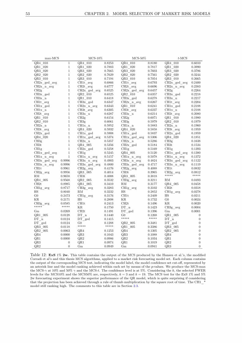
53 CHAPTER 2. MODEL SELECTION OF MARKET RISK MODELS
max-MCS MCS-10% MCS-50% t-MCSQR4_010 1 QR4_010 0.8253 QR4_010 0.8180 QR4_010 0.6010QR1_020 1 QR1_020 0.7883 QR1_020 0.7817 QR1_020 0.3990QR3_020 1 QR3_020 0.7665 QR3_020 0.7603 QR3_020 0.3786QR2_020 1 QR2_020 0.7629 QR2_020 0.7561 QR2_020 0.3244QR3_010 1 QR3_010 0.7194 QR3_010 0.7054 QR3_010 0.2665CH2x_ged_avg 1 CH1t_avg 0.6866 CH1t_avg 0.6793 CH2x_ged_avg 0.2400CH2x_n_avg 1 CH2t_avg 0.6777 CH2t_avg 0.6696 CH2x_n_avg 0.2383CH2g 1 CH2x_ged_avg 0.6525 CH2x_ged_avg 0.6457 CH2g 0.2264CH3x_ged 1 QR2_010 0.6525 QR2_010 0.6357 CH3x_ged 0.2218CH3x_n 1 QR1_010 0.6418 CH3x_ged 0.6278 CH3x_n 0.2217CH1t_avg 1 CH3x_ged 0.6347 CH2x_n_avg 0.6267 CH1t_avg 0.2204CH1x_ged 1 CH2x_n_avg 0.6343 QR1_010 0.6241 CH1x_ged 0.2188CH1x_n 1 CH3t_avg 0.6305 CH3t_avg 0.6237 CH1x_n 0.2188CH2t_avg 1 CH3x_n 0.6287 CH3x_n 0.6214 CH2t_avg 0.2080QR1_010 1 CH2g 0.6154 CH2g 0.6071 QR1_010 0.1980QR2_010 1 CH3g 0.6061 CH3g 0.5979 QR2_010 0.1979CH2x_n 1 CH1x_n 0.5952 CH1x_n 0.5883 CH2x_n 0.1960CH3t_avg 1 QR4_020 0.5932 QR4_020 0.5858 CH3t_avg 0.1959CH2x_ged 1 CH1x_ged 0.5908 CH1x_ged 0.5837 CH2x_ged 0.1959QR4_020 1 CH1x_ged_avg 0.5374 CH1x_ged_avg 0.5306 QR4_020 0.1851CH3g 1 CH2x_n 0.5357 CH2x_n 0.5286 CH3g 0.1638CH3t 1 QR4_005 0.5356 CH2x_ged 0.5184 CH3t 0.1534CH1g 1 CH2x_ged 0.5258 CH1g 0.5169 CH1g 0.1393CH1x_ged_avg 1 CH1g 0.5245 QR4_005 0.5120 CH1x_ged_avg 0.1380CH1x_n_avg 1 CH1x_n_avg 0.5157 CH1x_n_avg 0.5078 CH1x_n_avg 0.1372CH3x_ged_avg 0.9996 CH3x_n_avg 0.4903 CH3x_n_avg 0.4824 CH3x_ged_avg 0.1122CH3x_n_avg 0.9996 CH3x_ged_avg 0.4800 CH3x_ged_avg 0.4717 CH3x_n_avg 0.1119CH1t 0.9961 CH2g_avg 0.4176 CH2g_avg 0.4088 CH1t 0.0832CH2g_avg 0.9956 QR3_005 0.4014 CH3t 0.3965 CH2g_avg 0.0812RM 0.9658 CH3t 0.4008 QR3_005 0.3818 ***** *****QR4_005 0.9568 QR2_005 0.3532 CH3g_avg 0.3211 RM 0.0493CH2t 0.8985 QR1_005 0.3410 RM 0.3177 QR4_005 0.0458CH1g_avg 0.8717 CH3g_avg 0.3283 CH1g_avg 0.3102 CH2t 0.0318HS 0.8040 RM 0.3232 HS 0.2852 CH1g_avg 0.0278G0 0.2473 CH1g_avg 0.3176 CH1t 0.2409 HS 0.0211KR 0.2171 HS 0.2898 KR 0.1732 G0 0.0024CH3g_avg 0.0585 CH1t 0.2413 CH2t 0.1496 KR 0.0020***** ***** KR 0.1750 DT_n 0.1423 CH3g_avg 0.0004Gm 0.0269 CH2t 0.1491 DT_ged 0.1396 Gm 0.0001QR1_005 0.0128 DT_n 0.1440 G0 0.1268 QR1_005 0DT_n 0.0124 DT_ged 0.1415 ***** ***** DT_n 0DT_ged 0.0124 G0 0.1288 QR2_005 0.3481 DT_ged 0QR3_005 0.0118 ***** ***** QR1_005 0.3386 QR3_005 0QR2_005 0.0063 QR4 0.1253 QR4 0.1305 QR2_005 0QR4 0.0000 QR3 0.1043 QR3 0.1088 QR4 0QR1 0.0000 QR2 0.0986 QR2 0.1034 QR1 0QR3 0 QR1 0.0974 QR1 0.1019 QR2 0QR2 0 Gm 0.0949 Gm 0.0941 QR3 0
Table 12: ExS 1% 2w. This table contains the output of the MCS produced by the Hansen et al.’s, the modifiedCorradi et al’s and this thesis MCS algorithms, applied to a market risk forecasting model set. Each column containsthe output of the corresponding MCS test, indicating the model label, the model confidence set cut-off, represented byan asterisk line and the model ranking achieved within each set by means of the p-values. We produce the MCS-maxthe MCS-γ at 10% and 50% γ and the MCS-t. The confidence level is at 5%. Considering the k, the selected FWERlevels for the MCS10% and the MCS50% are, respectively, k = 3 and k = 19. The MCS test for the ExS 1% and 5%2w forecasting experiment shows the superior performance of the QR model, which is quite surprising if consideringthat the projection has been achieved through a rule of thumb multiplication by the square root of time. The CH1_*model still ranking high. The comments to this table are in Section 2.3.
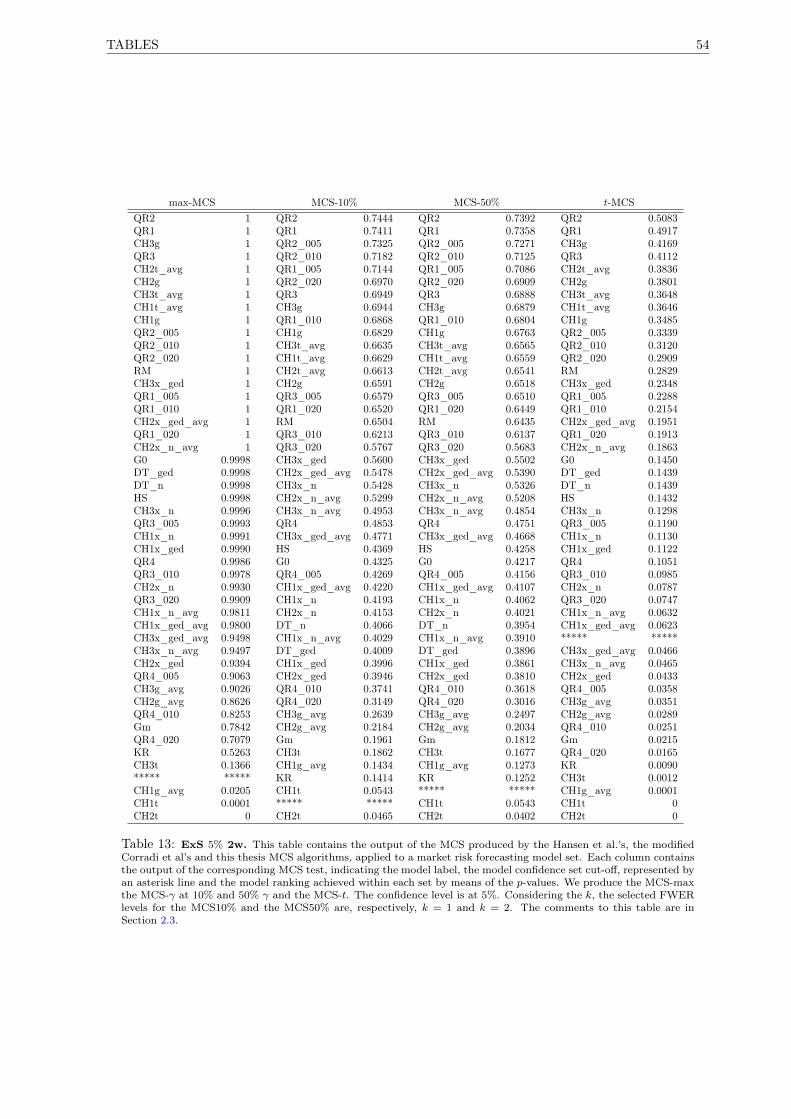
TABLES 54
max-MCS MCS-10% MCS-50% t-MCSQR2 1 QR2 0.7444 QR2 0.7392 QR2 0.5083QR1 1 QR1 0.7411 QR1 0.7358 QR1 0.4917CH3g 1 QR2_005 0.7325 QR2_005 0.7271 CH3g 0.4169QR3 1 QR2_010 0.7182 QR2_010 0.7125 QR3 0.4112CH2t_avg 1 QR1_005 0.7144 QR1_005 0.7086 CH2t_avg 0.3836CH2g 1 QR2_020 0.6970 QR2_020 0.6909 CH2g 0.3801CH3t_avg 1 QR3 0.6949 QR3 0.6888 CH3t_avg 0.3648CH1t_avg 1 CH3g 0.6944 CH3g 0.6879 CH1t_avg 0.3646CH1g 1 QR1_010 0.6868 QR1_010 0.6804 CH1g 0.3485QR2_005 1 CH1g 0.6829 CH1g 0.6763 QR2_005 0.3339QR2_010 1 CH3t_avg 0.6635 CH3t_avg 0.6565 QR2_010 0.3120QR2_020 1 CH1t_avg 0.6629 CH1t_avg 0.6559 QR2_020 0.2909RM 1 CH2t_avg 0.6613 CH2t_avg 0.6541 RM 0.2829CH3x_ged 1 CH2g 0.6591 CH2g 0.6518 CH3x_ged 0.2348QR1_005 1 QR3_005 0.6579 QR3_005 0.6510 QR1_005 0.2288QR1_010 1 QR1_020 0.6520 QR1_020 0.6449 QR1_010 0.2154CH2x_ged_avg 1 RM 0.6504 RM 0.6435 CH2x_ged_avg 0.1951QR1_020 1 QR3_010 0.6213 QR3_010 0.6137 QR1_020 0.1913CH2x_n_avg 1 QR3_020 0.5767 QR3_020 0.5683 CH2x_n_avg 0.1863G0 0.9998 CH3x_ged 0.5600 CH3x_ged 0.5502 G0 0.1450DT_ged 0.9998 CH2x_ged_avg 0.5478 CH2x_ged_avg 0.5390 DT_ged 0.1439DT_n 0.9998 CH3x_n 0.5428 CH3x_n 0.5326 DT_n 0.1439HS 0.9998 CH2x_n_avg 0.5299 CH2x_n_avg 0.5208 HS 0.1432CH3x_n 0.9996 CH3x_n_avg 0.4953 CH3x_n_avg 0.4854 CH3x_n 0.1298QR3_005 0.9993 QR4 0.4853 QR4 0.4751 QR3_005 0.1190CH1x_n 0.9991 CH3x_ged_avg 0.4771 CH3x_ged_avg 0.4668 CH1x_n 0.1130CH1x_ged 0.9990 HS 0.4369 HS 0.4258 CH1x_ged 0.1122QR4 0.9986 G0 0.4325 G0 0.4217 QR4 0.1051QR3_010 0.9978 QR4_005 0.4269 QR4_005 0.4156 QR3_010 0.0985CH2x_n 0.9930 CH1x_ged_avg 0.4220 CH1x_ged_avg 0.4107 CH2x_n 0.0787QR3_020 0.9909 CH1x_n 0.4193 CH1x_n 0.4062 QR3_020 0.0747CH1x_n_avg 0.9811 CH2x_n 0.4153 CH2x_n 0.4021 CH1x_n_avg 0.0632CH1x_ged_avg 0.9800 DT_n 0.4066 DT_n 0.3954 CH1x_ged_avg 0.0623CH3x_ged_avg 0.9498 CH1x_n_avg 0.4029 CH1x_n_avg 0.3910 ***** *****CH3x_n_avg 0.9497 DT_ged 0.4009 DT_ged 0.3896 CH3x_ged_avg 0.0466CH2x_ged 0.9394 CH1x_ged 0.3996 CH1x_ged 0.3861 CH3x_n_avg 0.0465QR4_005 0.9063 CH2x_ged 0.3946 CH2x_ged 0.3810 CH2x_ged 0.0433CH3g_avg 0.9026 QR4_010 0.3741 QR4_010 0.3618 QR4_005 0.0358CH2g_avg 0.8626 QR4_020 0.3149 QR4_020 0.3016 CH3g_avg 0.0351QR4_010 0.8253 CH3g_avg 0.2639 CH3g_avg 0.2497 CH2g_avg 0.0289Gm 0.7842 CH2g_avg 0.2184 CH2g_avg 0.2034 QR4_010 0.0251QR4_020 0.7079 Gm 0.1961 Gm 0.1812 Gm 0.0215KR 0.5263 CH3t 0.1862 CH3t 0.1677 QR4_020 0.0165CH3t 0.1366 CH1g_avg 0.1434 CH1g_avg 0.1273 KR 0.0090***** ***** KR 0.1414 KR 0.1252 CH3t 0.0012CH1g_avg 0.0205 CH1t 0.0543 ***** ***** CH1g_avg 0.0001CH1t 0.0001 ***** ***** CH1t 0.0543 CH1t 0CH2t 0 CH2t 0.0465 CH2t 0.0402 CH2t 0
Table 13: ExS 5% 2w. This table contains the output of the MCS produced by the Hansen et al.’s, the modifiedCorradi et al’s and this thesis MCS algorithms, applied to a market risk forecasting model set. Each column containsthe output of the corresponding MCS test, indicating the model label, the model confidence set cut-off, represented byan asterisk line and the model ranking achieved within each set by means of the p-values. We produce the MCS-maxthe MCS-γ at 10% and 50% γ and the MCS-t. The confidence level is at 5%. Considering the k, the selected FWERlevels for the MCS10% and the MCS50% are, respectively, k = 1 and k = 2. The comments to this table are inSection 2.3.

55 CHAPTER 3. MODEL SELECTION OF JUMP-DIFFUSION MODELS
Model Selection of
Jump-Diffusion Models
With the model selection experiment of this chapter, we are interested in the econometric analysis
of a large class of stochastic models, capable of matching observed financial market data characteristics.
This chapter is focused on parametric model families that are designed to capture the historical equity
stock price return dynamics. The model set is large enough to mimic the stylised features of the time
series as evidenced in the literature. We focus on single factor stochastic volatility models and restrict the
exercise to a suite of model types that are tested on several nested layers. A core challenge with any such
model specification analysis is the performance of the estimation procedures in the presence of insufficient
information, as the equity volatility is unobservable. As presented in Section 3.1, the observable variable,
that is the equity stock return is assumed to be given as a linear function of a set of stochastic inputs that
are either partially or completely unobserved. Specifically, we consider a jump-diffusion system which is
characterised by a latent component that enters either the stochastic diffusion or the stochastic inten-
sity driving the jump process. The benchmark model is represented by the stochastic volatility model
of Heston (1993), which is extended in several directions and compared with a non conventional model

56
family. The Heston model and, in general, the affine model class have gained popularity and widespread
use since their formalisation in Duffie and Kan (1996), Duffie et al. (2000) and Dai and Singleton (2000).
This model class provides a convenient tool for capturing stochastic volatility, an important statistical
characteristic of financial time series, at the same time allowing a certain ease of use due to the an-
alytic form of their moment generating function. However, the single factor stochastic volatility SDE
usually applied to model equity stocks can produce distributions with strong kurtosis only under extreme
parameter configurations and in general can generate a very moderate skew. Incremental kurtosis can
be achieved with the extension by an incremental parameter to trigger the elasticity of variance in the
constant elasticity of variance (CEV) model specification, used in Beckers (1980), Macbeth and Merville
(1980) and in a stochastic volatility context in Jones (2003) and Aït-Sahalia and Kimmel (2007). The
introduction of jump components also increases the flexibility of the model in adapting to observed return
distributions. In this regard, it is customary in finance to use jumps to explain rare events and usually
the estimations provided concerning the jump frequency and size vary from one to nine jumps per year,
with a negative average size of −3%, see Andersen et al. (2002), Eraker et al. (2003), Chernov et al.
(2003) and Pan (2002). In Section 3.1 and Appendix A.4, we provide more information concerning the
model details and their use in the literature. In this study, we counterbalance this application of the
jump component by extending the model set with a class of stochastic hazard models that employs high
frequency jumps in modelling financial time series. In this perspective, rare large jumps should be viewed
as tail events of frequent small jumps, as opposed to the standard paradigm that jumps are rare events
overall. The further major feature of this alternative model class, however, is that it is capable of gen-
erating stochastic volatility by combining frequent jumps and stochastic intensity, whereby the volatility
clustering is produced by peaks of the frequency of jumps.
The model selection exercise is conducted in two different environments. In the first test environment,
we arrange a simulation exercise to analyse the model ability in reproducing the sample characteristics
of a known DGP by testing the model performance with respect to the target estimation functions. The
purpose of this experiment involves testing the capacity of the models in reproducing each other’s charac-
teristics and hence provide alternative formulations for the econometric problem of interest. Specifically,
we compare CEV stochastic diffusive models equipped with rare large jumps that occur in the returns
process with constant intensity, a model class we indicate as the stochastic diffusion (SD) family, whereas
the alternative class of models contains constant diffusion models with high intensity of small jumps
characterised by stochastic hazard1 (SH). Both classes allow for constant intensity asynchronous jumps
in the latent factor. The complexity of the exercise is increased by the fact that the larger models within
each class are themselves affected by aliasing among their components. The use of simulation allows
the control of the sample features, whereby we have chosen to balance between the contribution to the
data variability of the diffusion and the jump component, whenever the latter is present. This simulation
parameters setting means that the unconditional variances of the diffusion and the jump component,
which sum up to the total model unconditional variance, are programmed to be equal. In particular
1 Two parametric models are nested if one can be derived from the other one by simply varying the parameters. Althoughthere is a possibility for nesting the two model classes, this modelling choice is prevented and the nesting class (i.e. themodel that is characterised simultaneously by CEV stochastic diffusion and CEV stochastic intensity, both driven by thesame latent component) is excluded.

57 CHAPTER 3. MODEL SELECTION OF JUMP-DIFFUSION MODELS
though, the variance produced by a jump component in the SD class is determined by rare large jumps,
whereas the variance produces by a jump component in the SH class is determined by very frequent small
jump. With the SH family we investigate a model whereby the volatility clustering can be generated by
the jump component solely. The motivation as to why we choose to include the SH family in the model
selection exercise and expand the overarching CEV class, is mainly scientific. This class has received
no attention in the applied finance literature. However, discrete time models that are at the foundation
of the econometrics discipline, can be viewed as high intensity jump models with non stochastic jump
times. Furthermore, the full record of the daily transactions on a typical trading day for a liquid financial
asset is intrinsically an high frequency stochastic intensity jump price sample. In the second test envi-
ronment, we produce a market data experiment whereby we test the model set performance and draw
inferences on real financial time series. The model set and estimation procedures applied to real market
data, complemented with tests of model comparison, reveal information useful for empirical researchers.
Concerning the test statistics, within the simulation test environment, they are produced with Monte
Carlo, whereas within the market data test environment, the market sample data are resampled with the
stationary bootstrap. The simulated experiment is suited for the application of a relative model compar-
ison test, whereby the suite of models is tested against the benchmark generating the sample data. A
relative model comparison is also arranged for the market data experiment, where the MHT is structured
to circulate the benchmark across the model set. The relative model comparisons expose the detail of
the preferences among individual models induced by the statistical test and reveal the full collection of
equivalence hypotheses. Finally, we explore the absolute model performance, whereby MCS tests are
applied to the data set to draw general conclusions regarding model superiority. Exploiting the flexibility
of the approach of Section 1.1 and Section 1.3, we deliver MCS tests of the performance of jump-diffusion
(JD) models targeting the historical measure of an equity index log-levels. The model comparisons are
based on the max -MCS of Hansen et al. (2011), as constructed in Section 1.3.1, our new t-MCS inspired
by Corradi and Distaso (2011), as constructed in Section 1.3.2, and the novel γ-MCS, of Section 1.3.3,
combining the MCS and the MHT framework.
The econometric analysis of the historical measure of equity stock indices by means of stochastic volatility
JD models is pursued in articles such as Andersen et al. (2002), Chernov et al. (2003) and Eraker et al.
(2003). These articles, however, lack of a direct model comparison statistical procedure, whereby the
model pairwise confrontation is at most achieved by comparing the EMM χ2 statistics, or pursued with
the approach of the Bayesian factors, which is not strictly based on hypothesis testing, but is rather a
relative measure of the likelihood of a model. The contribution of this study is original as the model
selection analysis is achieved explicitly via joint statistical testing targeting several measures of model
performance. This chapter provides several contributions. First, we test the model aliasing hypothesis
among two alternative classes of jump-diffusion models, namely the conventional affine stochastic volatil-
ity model class popular in the literature and the non-conventional stochastic hazard model class, that
exhibit the ability to generate similar empirical time series features and that heretofore have not been
pitted against each other in the literature. Second, we provide new insights into the stochastic hazard
class, with the market data experiment showing such models to be highly ranked in performance. Third,
we uniquely design and implement model comparison tests under recent and novel testing approaches, ex-

58
ploiting multiple hypothesis testing and the model confidence set techniques. Such techniques are ideally
structured to allow us to explore the model aliasing hypothesis. Finally, as a methodological extension
specific to this chapter, we extend the second order filtering procedure in Maybeck (1982) to allow jump
components in the system state. The general information that we gather from the experiments of this
study shows that the main model families exhibit strong aliasing and can produce similar features, with
respect to the model performance measures. The fact that the models can in principles be each other sub-
stitutes, makes the market data experiment outcome more significant, whereby a particular alternative
model reveals superior performance than the more conventional ones. This behaviour indicates that some
SH models exhibit larger flexibility as they can structurally resemble the behaviour of SD models, at the
same time producing distinctively top range performance in mimicking market data. On the other hand,
the CEV model class delivers interesting performances and, specifically with respect to the likelihood
performance measure, points to a simplified model structure in preference over more complex structures.
The chapter is organised as follows. In Section 3.1 we introduce the model set and define the general
stochastic differential equation (SDE) describing the model components in Eqs. (3.1), (3.2), discussing
also the general behaviour of the system. In Appendices A.1 to A.3 we detail the algorithms necessary
for the parameter and latent state estimation, as well as the calculation of the performance measures by
which the model selection exercise is addressed. Section 3.2 discusses the testing framework and presents
the relative loss function defined upon the output of the likelihood function and the filtering procedure.
Section 3.3 elucidates on several operational aspects of the exercises of this chapter and proposes a light
comparison exercise between the filter technique employed in this work and a particle filter. The re-
mainder of the latter section presents the results of the various experiments with simulated and financial
market data. Section 3.4 gathers conclusions. The Appendix A collects several technical aspects con-
cerning the analytics used throughout the article, whereas Appendix B provides more details about the
implementation of the algorithms by which the experiments have been assembled.
Some clarifications
In econometrics, the aliasing effect is usually referred to the loss of information arising when discretely
sampling continuous time processes. Specifically, the term originates from the theory of signals and refers
to the lack of identifiability of the ω + 2πk, k ∈ Z frequencies, as they will all appear to have frequency
ω, cfr. for instance Priestley (1981). As a consequence, it might occur that two processes with the same
sample spectra could differ in frequencies that cannot be observed because of the discrete data and thus
be indistinguishable, from a statistical perspective. Another phenomenon that has been referred to as
aliasing in econometrics, for instance, is the problem of estimating the parameters of the diffusion and the
jump component in a jump-diffusion process, cfr. Aït-Sahalia (2004). The author of that study provides
interesting intuition as to why the aliasing arises. In fact, for the reference Merton model, it is shown
that suitably changing the diffusion and jump components’ parameters, it is possible to obtain a fixed
measure of the shape distribution, such as, for example, the variance or the kurtosis. Another interesting
point is the rapidly decreasing probability of detecting a jump, when the sampling interval increases.
Analytic results are obtained with respect to the simple prototype model, which show that the likelihood

59 CHAPTER 3. MODEL SELECTION OF JUMP-DIFFUSION MODELS
can asymptotically detect the diffusion coefficient without the interference due to the presence of jumps,
as long as the process is sampled at very short time intervals. Notwithstanding those results carried over
an analytically tractable model, the asymptotic moments remain entangled with both diffusion and jump
coefficients and therefore anticipating uncertainty when using the GMM.
In this thesis chapter we employ the term aliasing in a wide context, referring to model performances
that are confusing in the sense that models that are structurally different produce similar outcomes. The
sources of aliasing might be multiple. The models are expected to be misspecified or are rather misspeci-
fied by construction and the system is assumed to be partially observed. The point of testing for aliasing
with simulation is as follows. Assume, for instance, we have two nested models. The question is to which
extent the nested one is statistically equivalent to the overarching model when the former is adapted to
a sample which is generated by the latter. We would expect that, foremost, the answer depends on the
model performance measure. In particular, we are targeting a marginalised likelihood and the projection
of the latent system state with an approximated non-linear filter, two measures that are constructed on
a partial information set. We notice, for instance, that jump-less models hardly match discontinuous
paths, whereas jumps in volatility have a more elusive sample feature. The exercise is limited in the
sense that we only consider an affine SD family and a disjoint SH family hinging on the prior that the
volatility clustering is produced by frequent small jumps hitting the system with stochastic intensity. A
CEV extension is also considered, as well as several jump specifications. Another interesting result of the
simulation is the very flexible performance of the SH models, that are among the top performers in the
real market data exercise, as long as a good performing CEV specification is in place.
For the purpose of model selection, we distinguish the problem of parametrising the statistical distribu-
tion of the model set from that of filtering the latent state component, as we employ two procedures that
target respectively and distinctively the likelihood of the observable and the projection of the unobserved
component. The estimates are then used to perform computations and to evaluate model performance.
We exploit an approximation of the likelihood function to estimate the model parameters that involves
the marginalisation of the unobservable variable, whereas the path of the latent component is estimated
through a filtering procedure which receives the model parameters as an input. The focal point of the
analysis is the comparison of possibly misspecified models acting in a context of partial information,
whereby their performance is measured in terms of the information they are capable of extracting from
sample data, both from a distributional as well as from a dynamic behaviour perspective. The loss
functions defining the model comparison statistics therefore measure the ability of the model in match-
ing the sample information and therefore reproducing the distributional characteristics of the observed
system and the ability of the model in inferring the dynamic behaviour of the latent components. The
measures for model comparison are derived directly from the likelihood function and from the filtering
algorithm. Despite the different objectives of the estimation approaches2, they share a common origi-
nation in the forward equation, that is the partial integral-differential equation (PIDE) describing the
transition density of the system. The inner component of the likelihood function is constructed as the2 The procedure of marginalisation of the latent component has been developed primarily to target the likelihood of
the observed data, insulating the further complication of estimating the unobservable variable into a distinct computation.Incidentally, the algorithm improves the computational charge.

60
numerical solution of the forward equation and, combined with the marginalisation procedure, is used
for the parameter estimation and to derive information theoretic loss measures. The filtering technique
of Maybeck (1982), Nielsen et al. (2000), Baadsgaard et al. (2000), also used in Hurn et al. (2013), is
constructed as a projection onto the observable set of information. The filtered latent path feeds either
measures of path-wise distance or a joint likelihood loss indicator. Exploiting the procedure by which
the (diffusion only) propagation equation is derived, we extend the filter by including a jump element
that allows one to deal with more general JD models, as we pursue here. This jump-augmented filtering
approach is another of the main contributions of this chapter. The form of the jump that the filter
can handle is quite general, including synchronous or asynchronous jumps, state-dependent jump size
distributions along with affine as well as non-affine state-dependent jump-intensities.
The specific statistical entanglement and the effects of truncation errors related to the algorithms em-
ployed are not subjects of research, as we focus on the application of the bootstrap methodology and
the MHT-MCS framework to explore model similarities and superior performances in simulated and real
data experiments. However, we pinpoint here several issues left for further examination. The analysis is
executed with approximate maximum likelihood estimation methods, that is the likelihood of the chosen
model is not known in closed form and therefore numerical methods have been employed to generate the
estimation function. From a theoretical statistics point of view, the analysis can be set in the frame-
work of Poulsen (1999) whereby, assuming consistent and asymptotically normal estimates (CAN) of the
‘true’ likelihood, only second order precision of the AML is required to obtain CAN as well. On the
other hand, the AML can in general fall into the theory of misspecified models when the more practical
misspecification hypothesis is assumed, see White (1982, 1994). The study of the empirical behaviour of
the discretisation is beyond the scope of this thesis. Another complication of the analysis of this chapter,
which deserves a separate analysis, is represented by the partial observation of the system state, entailing
the exploitation of filtering techniques to measure the expected path of the latent component. We resort
to an approximated non linear filter, which we trace back to Maybeck (1982). The peculiar feature of the
filter is that it can disregard the estimation of the prior distributions, as it only requires the evolutionary
equations of the latent state projections and provides a direct expression for the evolutionary equation of
the system projection. To obtain an ordinary differential equation that can be employed for computation,
the ODE can be expanded in some terms that involve the expectation operator, effectively rendering a
second order approximated filter3. As a consequence of the higher order expansion, the estimate of the
system state transition expectation is adjusted by a bias correction term. However, some crude estimation
is then used when the observation density is required, in practice resorting to a (first order approximated)
non linear least square of the expected posterior value. The consequences of these practical remedies in
terms of precision of the estimates and possible improvements, deserve further research. A point we make
is that we do not use the likelihood of a possible observation error in order to estimate the system param-
eters. In many simulation we do not report, the peculiar form of the system state which hosts already
the observed variable, determines some odd behaviour of the latent state projection, as indeterminacy
is already captured by the diffusion and possibly the jump component. Furthermore, this approach has
been proved to be distorted, as the observation error exhibits high correlation with observable, as well as
3 It has to be noticed that for affine and quadratic models the time-propagation equation is exact.

61 CHAPTER 3. MODEL SELECTION OF JUMP-DIFFUSION MODELS
autocorrelation, see for instance Dempster and Tang (2011).
3.1 The Jump-Diffusion Model Set
In this chapter, we restrict the attention to a jump-diffusion system, which is designed to capture many of
the stylised features of equity stock financial time series. The overarching model we consider is specified
by the following parametric SDE
dx = θvγ0dW0 + J0 dN0 −m0dt
dv = κ(1− v) dt+ σ√v dW1 + J1 dN1 −m1dt,
(3.1)
which represents a jump-diffusion family of models which is characterised by log-return process x and a
volatility process v, both driven by defined diffusive and jump factors. The volatility process v is defined
to evolve according to a square root process that can be affected by jumps, which may or may not be
synchronous with the jumps in the returns process. The jump process are defined by the following two
jump-related differentials describing jump arrival intensity:
dΛ0 = λ0v2γ1dt
dΛ1 = λ1dt(3.2)
These are the hazard functions of the compounded Poisson jumps N0 and N1. The stochastic factor
can enter either the constant elasticity4 of variance (CEV) diffusion in x or the CEV stochastic hazard
function of N0, where we fix 0 ≤ γ0, γ1 < 1. The overarching model in Eq. (3.1) and (3.2) is intended
to mimic the behaviour of the log-price of and equity stock. The x process is not characterised by any
particular drift, which is expected to be null5. The model produces stochastic volatility, that is the
clustering of price variations into high and low volatility regimes and further instantaneous acceleration
of the price achieved through jump in level and possibly sudden spikes in volatility generated by jumps
in the latent factor. As we allow for high frequency small jumps, the stochastic volatility can be gen-
erated by either a higher diffusion factor or by a peak in the number of jumps. The clustering of the
returns is determined by the mean reversion feature of the latent factor, which exhibits some viscosity
in pulling back to the long run level from a spike. We do not mix stochastic diffusion and stochas-
tic intensity models, thus if γ0 6= 0 ⇒ γ1 = 0 and viceversa. We make this choice as in the present
study we exploit jump models with random jump frequency in an alternative fashion, allowing for an
high intensity self-exciting system that uses the latent stochastic hazard function to generate stochastic
volatility. The suggested hypothesis that is complementary is that combining stochastic diffusion and
stochastic intensity determines an overidentifying restriction. Hence, the intensity of the jumps in x are
either constant or random, whereas the intensity of the jump in the v factor is constant. The latter
is the one that is considered latent in the simulation or is unobservable or partially observable in the
4 In economics, the elasticity of the function U(c) is defined as −cU ′′/U ′. This corresponds to an elasticity of the functionvγ of 1− γ.
5 Contrary to market practice in defining log-transform models of affine stochastic volatility, we drop here the Jensenterm that would result from the transformation of the price martingale, as the perspective that we take is mainly that ofthe historical data. As explained in the Appendix A.4, employing a log-return model with a stochastic volatility drift termshould be justified by autocorrelation in the first difference of the data, which is not the case, see also Bollerslev and Zhou(2002).

3.1. THE JUMP-DIFFUSION MODEL SET 62
market-data experiment. In term of parameters, we observe that we apply some simple transformations
to popular versions of the model subcomponents, see Appendix A.4, to obtain a latent factor v that
oscillates around a unitary mean, with mean reversion factor κ. The diffusion of the square root factor
is determined by the parameter σ, whereas the jump component J1dN1 is compensated by the drift
adjustment m1dt; the constant intensity is λ1. The latent factor enters either the diffusion of x, whereby
it is scaled by θ and exponentiated by γ0, which in the non CEV version is fixed to one half, or it enters
the intensity function of the jump in return process J0dN0, whereby it is scaled by the parameter λ0
and exponentiated by γ1, which in the non CEV version is fixed to one half and in the SD model class
is fixed to zero. The jumps compensation drifts m0 and m1 are constant. The mean reversion speed is
requested to be higher than the jump drift and their difference greater than half the squared diffusion
coefficient, that is β −m1 >σ2
2 > 0, in order to obtain stationary variance, at the same time preventing
the crossing of the zero level6. We allow for the presence of correlated diffusive random drivers7 between
the factor x and the stochastic volatility factor v, that is d[W0,W1] = ρdt, the so called leverage effect,
a phenomenon witnessed at least since Schmalensee and Trippi (1978) and modelled, for instance, in
Glosten et al. (1993). If jumps in v are included, their expectation is required to be greater than one,
cfr. (A.2) in Appendix A. The jump size distribution J1 of the Poisson point process component in v
is specified as a positive exponential, whereas in the case of N0 a negative exponential jump is specified
in the stochastic diffusion case, with constant jump intensity. A double-exponential distribution or a
skewed normal jump is employed with the stochastic hazard model version of x, whereby in this case
the jump size is constrained to a zero expected value. Moreover, we notice that the stochastic hazard
family is not affine, as the covariance matrix of the diffusion component cannot be written in a linear form.
The models of the exercise in this chapter are organised into two major families, exhibiting stochastic
volatility that is generated either by the diffusion factor, the SD class, or by the jump intensity of the
Poisson component of the cumulative return process, the SH class. In fact, both the stochastic diffusion
and the stochastic jump intensity version of the overarching model in Eqs. (3.1), (3.2) are stochastic
volatility models, as it can be seen by taking their quadratic variation given by the v-dependent stochas-
tic integral∫
dt[θ2v2γ0 + λ0v
2γ1EJ20
]. The volatility clustering which characterises diffusive stochastic
volatility models can be also produced by intensively jumping stochastic hazard models, which entails
a concentration of larger variations of x during volatility peaks. In the case of the CEV version of the
SH family, the γ0 parameter will exacerbate this feature, for higher parametric values. The stochastic
hazard models are characterised by high frequency jump intensity on average, whereas models of the
stochastic diffusion class that manifest jumps in the level of the observable variable are expected to
jump less frequently. A minor distinction between the stochastic diffusion and the stochastic hazard
6 We will sometimes refer to the ratio σ2
2(β−m1), as the volatility excursion factor. It should be between zero and one,
whereby values close to the unity determine very spiked volatility paths, that is large excursion, whereas values close tozero entails that v rarely leaves a neighbourhood of the long-run level.
7 This feature produces a bidimensional diffusion which tends to associate negative variations in x with increasing v andviceversa, but not necessarily couples large negative variations in x with peaks in volatility and the other way around,therefore producing only slight asymmetry in the marginal density of the observable x. That is to say, the correlateddiffusion W0 and W1 do not produce higher volatility in the presence of negative trends in the price level, but they tend toassociate negative returns with growing volatility, a feature that might happen at low levels of volatility as well. Therefore,affine models are not expected to produce strong asymmetry via the ρ coefficient. In practice, if were, for instance, to seta simulation of a correlated affine stochastic volatility model, we would observe that the first difference of x be correlatedwith the first difference of v but not with its level. From the simulation, we observe that in the presence of negative orbidirectional jumps, the likelihood manifest a strong aliasing between the correlation coefficient and the latter component.

63 CHAPTER 3. MODEL SELECTION OF JUMP-DIFFUSION MODELS
classes lies in the direction of the jumps of x, if any, which is negative in the former case, whereas it it
can be positive or negative in the latter case. From a distributional perspective this feature entails that
the SD class can only produce negative symmetry that is the case of interest for market data applications.
The system in (3.1) contains or can be connected with several popular models used in financial econo-
metrics applications, although not all of them are employed in the analysis here and in general some
subcomponents are disconnected in order to obtain models exhibiting similar features but that are struc-
turally different. Indeed, as the scope of this analysis covers discriminating among stochastic models in
terms of explanatory power, the inclusion of an overall nesting model would not add any insight to the
final result, because the overall nesting model would be capable of matching any behaviour of its compo-
nents. One of the hypotheses we are investigating in the market data experiment consists in whether one
of the model class is superior. The connection with popular models is only illustrative. Correspondence
of the overarching model to model specifications prominent in the financial literature is shown in Tab.
15. However, a full illustration of the transformations needed to obtain more conventional models used
in literature are presented in Appendix A.4. Parameters constraint associated to the latter models are
as follows. If we exclude both jumps in return and volatility and set γ0 = γ1 = 1/2 we get the seminal
stochastic volatility model of Heston (1993). Considering the jump in volatility and if the jump in x is
skewed normal with null parameter of asymmetry, we obtain the SVS(C)J model of Eraker (2004), with
uncorrelated jumps. If in the last model we set γ1 = 0, we obtain Eraker et al. (2003), also included in
Duffie et al. (2000), Bates (2000) and Pan (2002); if further zeroing λ1 = 0, we get Bates (1996), also in-
cluded in Duffie et al. (2000). If we leave γ0 free, set λ0 = λ1 = 0 we can obtain the CEV models in either
Beckers (1980) and Macbeth and Merville (1980) or Jones (2003) and Aït-Sahalia and Kimmel (2007).
If we then set γ0 = γ1 = 0 and consider the Gaussian determination of the skewed Normal jump distri-
bution, we get the Merton (1976) model, whereas with double-exponential jumps, we obtain the (Kou,
2002; Kou and Wang, 2004) model. Notwithstanding this established relation between the system in Eqs.
(3.1), (3.2), and these prominent models in the financial literature, in this work we compare reduced and
extended forms of these models to perform model comparison of conventional and unconventional models
of stochastic volatility. The model set is first tested in a simulated environment to check for fungible
characteristics. Successively, the model set is tested onto real market data to search for model superior
performance. This research has to date provided evidence to support the adequacy of these increasing
complicated model specifications, however, the work in this chapter is the first study to examine a wide
range of jump-diffusion models where it is conjectured that there is a strong aliasing among these mod-
els, and further among individual components of these models, which offers the possibility of simplifying
model structure, at least from an historical measure perspective. The trend in the literature has been
towards increasingly complicated model specifications in an effort to better capture market dynamics,
yet this comes at a cost in terms of increasing levels of estimation error and bias and, from a practitioner
perspective, increasing disconnect with the regulatory requirements of industry. The analysis presented
in this chapter offers new insights into the trade off between alternative model specifications using for the
first time a rigorous MCS approach, which is further complemented with a direct multiple comparison
test in the MHT testing, under the most general γ-MCS. The MCS approach taken here is ideally suited
for the investigation of model aliasing among the suite of models considered.

3.1. THE JUMP-DIFFUSION MODEL SET 64
3.1.1 Parameter Estimation
The parameter estimation of jump-diffusion models in quantitative finance has received extensive treat-
ment, in the latter two decades. Methods to pursue this task are varied. Without any claim of compiling
an exhaustive literary review on the topic, we recall the efficient method of moments of Gallant and
Tauchen (1996), the empirical characteristic function approach of Singleton (2001), the spectral GMM
of Chako and Viceira (2003). In the realm of the likelihood estimation, the methods to approximate the
likelihood relies on simulation, as in the simulated maximum likelihood of Pedersen (1995b) and its exten-
sions in Durham and Gallant (2002), or exploit the expansion of the transition density as in Aït-Sahalia
(1996, 1999, 2002, 2008) or alternatively use PIDE methods to solve the transition equation. Example
of the latter approach are Lo (1988), Poulsen (1999), Lindström (2007). In this study, we embrace an
approximate maximum likelihood (AML) method of this type as it has proved to be very general and
relatively easy to implement, with moderate computational costs. We favourite FDM to solve the main
PIDE as polynomial expansion methods deliver oscillatory solutions. Moreover, the likelihood approach
is theoretically the most efficient estimator and is characterised by a distinctive theory of model compar-
ison when the models are misspecified, see for instance Akaike (1974), White (1982). We use likelihood
methods for the parameter estimation of multivariate JDs with latent components, constructed as the
numerical solution of the forward equation (A.6) combined with the marginalisation of the latent factor
by weighting for its stationary density. Exploiting an approximate maximum likelihood approach, the
procedure acquires the inherent optimal properties of the exact likelihood that can be achieved asymp-
totically by the approximation, cfr. Pedersen (1995a), Poulsen (1999). The same result extends to the
PIDE version, provided uniform convergence of the solution, see Lindström (2007).
The likelihood function hinges on the marginal densities of the first difference of the x process, constructed
around the transition density of the state vector. Symbolically, the log-likelihood is represented by index
LN (Θ) = − 1N
N∑i=1
log Pδti ∆x = ∆xi|0x; Θ (3.3)
which provides the measure for the construction of multiple hypothesis model selection tests, as detailed
in Section 3.2. In the likelihood equation, ∆xi is the return over the time horizon δti and each likelihood
solution Pδti is centred at x = 0. For each model and sample data, the parameter vector Θ∗ that optimises
the data function (3.3), enters both the likelihood and the latent component loss functions. The main
steps toward the practical implementation of the likelihood estimation algorithm adopted in the model
comparison exercise are depicted in the Appendix A.1, which describes the logical step to achieve the
marginalisation of the latent variable and therefore obtain the likelihood of the observable variable, as well
as the setup for the approximation of the transition density. More information related to the numerical
solution of the PIDE equation of this problem are given in Appendix A.2, which presents the construction
of the solver by the FDM. The pseudo-code description of this algorithm is presented in Appendix B.1.

65 CHAPTER 3. MODEL SELECTION OF JUMP-DIFFUSION MODELS
3.1.2 The Second Order Non-Linear Filter
In order to analysis the performance of the model set with respect to the latent component problem,
we adopt the filtering technique of Maybeck (1982), employed in finance in applications such as Nielsen
et al. (2000), Baadsgaard et al. (2000) and Hurn et al. (2013). As an auxiliary contribution of this
work, we extend the second order non-linear filter (NLF2) augmenting the time-propagation equation
to include a jump component in the system. This approach is convenient and, in particular, it does
not require the solution of the PIDE associated with (3.1), relying instead on the transition equation of
the expectation function derived from the forward equation. In Appendix A.3 we present the particular
approach undertaken in the construction of the time-propagation equation of the filter, as well as the
jump extension introduced in this study. In the appendix we also illustrate the standard approach in
determining the update equation and explain the second order expansion by which non linear expectation
are dealt with in the application section. Appendix A.3 also exhibits some examples. As this solution
does not involve time expensive calculations, we can afford an increased system state dimension and hence
split the x variable into its main stochastic drivers, namely the diffusion and the jump component, further
introducing a new observable, that is the integrated variance. The integrated variance is an elaboration
of x which makes observable the cumulative second order moment of the return process. Specifically,
rearranging the system of Eq. (3.1) and introducing the auxiliary observable w, we concentrate the
analysis on the system
dξ = θvγ0 dW0 −m0dt
dv = κ(1− v) dt+ σ√v dW1 + J1 dN1 −m1dt
du = θ2v2γ0 dt
dπx = J0 dN0
dπw = J20 dN0
(3.4)
which represents the engine of the latent component estimation exercise. The system state in Eq. (3.4)
is augmented with the observable w = u + πw that represents the integrated variance. Moreover, the
state is rearranged in such a way that the diffusion and the jump components of the x and w observable
variables are projected explicitly. The observation equation is given by the linear form
x = ξ + πx
w = u+ πw(3.5)
which in the formalism described in Appendix A.3 corresponds to the observable vector Y = (x,w)> =[1 0 0 1 0
0 0 1 0 1
]X. With the system state X = (ξ, v, u, πx, πw)> we are isolating the random sources
into specific state variables, a choice of design that allows for the disentangling of the jump variable
from the diffusion component. As a consequence, the filter defined by the Eqs. (3.4) and (3.5) is able,
in particular, to produce the projection of the latent variable πx, which accumulates the jumps8 of the
observable x. We will use this filter output to estimate the jump times and sizes and to produce a simple
benchmarking exercise of the procedure used here with a particle filtering technique. A by-product of the
8 This strategy, however, cannot be directly implemented for the estimation of the jump component of the v factor, as itdoes not enter directly into any observable.
3.2. MODEL COMPARISON TESTING 66
filtering which might be of interest is the estimate of the path of the latent variable ξ and thus the total
variance attribution between the jump and diffusion component of x. Progressing with the construction
of the device needed for the second battery of model comparison tests, we have augmented the observable
with a new variable w, which plays a special role in the system economy. As the state vector (ξ, πx, v)
is completely unobservable with a dimension higher than that of x, we would expect a strong degree
of indeterminacy in estimating its projection. For this case study, however, we can resort to stochastic
calculus and obtain two new variables which increase the information content available by introducing a
new observable. We expand the system with the integrated variance of the process x, which is partially
observable. This system extension can be proved to be statistically significant. The integrated variance
has been used in other applications in a realised volatility context, see for instance Bollerslev and Zhou
(2002), which exploits its moment structure to improve the estimation of a stochastic volatility model,
see also Barndorff-Nielsen and Shephard (2002), Barndorff-Nielsen and Shephard (2004). In this work,
the origination point is different. We construct the process w considering the SDE which describes the
observable x = ξ + πx and derive the process dynamics for χ = x2
dχ = 2x (θvγ0 dW0 −m0 dt) + θ2v2γ0 dt+[(x− J0)2 − x2
]dN0
= 2x dx+ θ2v2γ0 dt+ J20 dN0
= 2x dx+ du+ dπw.
Hence, let w = x2 − 2∫x dx to obtain the new observable w = u+ πw. It is implicit that because of the
term 2∫xdx that can only be approximated, the variable w is subject to a measurement error which
is assumed to spill into the estimate of πw. We do not introduce further auxiliary variables interpreted
as observation errors because of the presence of several overlapping latent sub-components into which
the total system variance has to be attributed. A noisy observation error is redundant as it can easily
be blurred into the diffusion component or be considered as the leftover variance once the system jumps
have been isolated as tail events of the projected jump components, πx and πw, cfr. Section 3.3.
3.2 Model Comparison Testing
As anticipated in Section 1.4, for the experimental part of this chapter we devise an exercise of relative
model performance MHT, as defined in (1.2), targeting jump-diffusion models. The test exploits the
balanced simultaneous confidence set controlling for the k-FWER and augmented with a step-down algo-
rithm to further refine the subset of significantly equivalent models and increase the statistical power of
the test. The relative performance test is executed under the simulated scenario, whereby the structure of
the experiment is suited for this type of comparison. For each benchmark model, sample data is generated
and hence model performance measures are derived, after previous parametrisation and filtering. The
main purpose of the test is to explore the model ability in reproducing each other’s features exhibiting
greater flexibility with respect to the target loss functions. We also produce a relative model performance
MHT processing real market data, whereby, as the “true” data generating process is unknown, a bench-
marking iteration is used to scan thoroughly the precedence relationships across the full set of model
comparisons. The purpose of this exercise is mainly to be descriptive of the multivariate distributions of

67 CHAPTER 3. MODEL SELECTION OF JUMP-DIFFUSION MODELS
the model comparison statistics, which are thereafter synthesised and represented by the outcome of the
absolute model performance MHT. Final conclusions regarding the model selection exercise are drawn
by means of the max -MCS (Section 1.3.1), the t-MCS (Section 1.3.2) and the γ-MCS (Section 1.3.3)
performed with simulated and real data. With the simulated exercise, the set of the best equivalently
performing models can be regarded as the collection of models that are statistically similar to the selected
benchmark and can therefore be considered as substitutes. With the real market data experiment, we
search for the best set of models fitting the data in terms of the target functions, producing original
model selection results through the application of the MHT and the MCS. The reference model setM is
represented by stochastic volatility families described in Section 3.1.
The loss functions Lj ’s constructed for the sake of model comparison, exploit an information criterion as
well as the metric represented by the path-wise distance derived from the filtering procedure. The first
measures when combined into the model relative performance dij ’s give raise to likelihood ratios, which is
essentially a measure of fitting of the target empirical distribution. Moreover, as the latter is constructed
by integrating out the latent component, we investigate a further indicator of model performance, which
measures the model ability in producing superior projections of the unobservable component. For the
case of the real market experiment, we also construct a hybrid measure of model performance combining
the full approximate likelihood evaluated at the vector of parameter Θ∗i over the actual market returns
and the filtered volatility trajectory. Particulars of the loss functions are presented in the following para-
graphs. The AML algorithm and the augmented non-linear filter employed in this study are detailed in
Appendix A.1 and Appendix A.3.
The loss functions presented in this section are used in the empirical section to construct MHT with
step-down refinement relative performance test that are indicated as LR-MHT, LC-MHT, LRLC-MHT
and TG-MHT. Absolute performance tests are executed in the simulation environment, with respect to
each model sample, and in the market-data experiment, with respect to a well diversified large stock
index data, employing the (LR/LC/LRLC/TG)-MCS-max, the (LR/LC/LRLC/TG)-MCS-t and the
(LR/LC/LRLC/TG)-MCS-γ, defined as follows.
3.2.1 Likelihood Ratio
In the context of model specification analysis, a fundamental result is represented by the following limit.
Let z1, . . . , zn be n independent observations on a random vector z, with probability density function
g(z) and consider the family of models represented by the parametric family of densities fθ(z), θ ∈ Θ
with a vector parameter θ and parameter space Θ ⊂ Rk. The following limit holds almost surely
1n
n∑i=1
log fθ(zi)n−→∫
dz g(z) log fθ(z),
provided the last integral exists. Indicating with S(g; fθ) the latter limit integral, we can define the
Kullback-Leibler information criterion, which is a distance measure of the likelihood of the possibly
misspecified model from the true one, that is K := S(g; g) − S(g; fθ), cfr. White (1982, 1994) and Rao
3.2. MODEL COMPARISON TESTING 68
and Wu (2001). By the Cramer-Rao bound, K ≥ 0 with equality only if fθ ≡ g. The likelihood ratio
between model fθ and model hϕ is the difference
LR(g; fθ, hϕ) := S(g; fθ)− S(g;hϕ),
which represents the distance gap of the model candidates.
Concerning the model comparison experiments targeting the model likelihood, we define the loss function
as
Li := −Li (Θ∗i ) (3.6)
whereby the RHS refers to Eq. (3.3) and we have dropped the reference to the sample size and introduced
the model index i. The sign has been changed because in practice the objective function is minimised and
more importantly to comply with the definition of a loss function, as adopted in the context of the model
selection strategy in Section 1.1. As a consequence, the relative performance measure dij = Li − Lj
corresponds to the sample equivalent of the LR, which would signal model equivalence as long as its
value is not significantly different from zero. We refer to tests obtained from the loss function (3.6) as
the likelihood ratio test (LR).
3.2.2 Distance from the Latent Component
The second type of performance measure we employ is intended to detect the ability of a model to produce
a reliable projection of the latent system state variable v. The unobservable component projection is the
output of the NLF2 procedure developed in Appendix A.3 and applied to the system described in the
Eqs. (3.4) and (3.5). The performance indicator that is used with this battery of test focuses solely on the
filter output, which by construction does not involve the likelihood function to produce the latent state
estimate. The test is intended to measure the model ability in describing the evolution of the system, with
particular reference to the inferred unobservable variable v. The test is centred on the latent stochastic
driver v as it is common to the full model set. Some measures of the jump-time hit rate are reported as
descriptive quantities of the filter algorithm performance in the filter benchmarking exercise of Tab. 30
as illustrated in Section 3.3.1.1. The loss function is obtained as the absolute distance of either the latent
variable projection from the actual path of v for each benchmark sample in the simulation exercise, or
of the appropriately scaled and translated latent variable projection from a threshold GARCH estimate,
cfr. Glosten et al. (1993), of the financial returns volatility, in the real data experiment. In the latter
case, with the experiment involving financial market data, we fix the lack of knowledge of the v path
by linking the filter output to the GARCH model that in econometric applications has been used as a
financial return volatility proxy for decades, see for instance Engle (1982) and Bollerslev (1986), Nelson
(1991) and Hansen and Lunde (2005). However, although employing observable data, the autoregressive
conditional heteroskedastic model offers a term of comparison only indirectly related to the system state
projection9.
9 The ratio of the overall average of the absolute path distance of the scaled and translated filter output from the standarddeviation of the GARCH filter is 17.25%

69 CHAPTER 3. MODEL SELECTION OF JUMP-DIFFUSION MODELS
Indicating with ν the reference latent system state path, the loss function of the model Pi is
Li = 1N
N∑j=1
∣∣∣vitj − νtj ∣∣∣ (3.7)
In the loss function (3.7), when referred to the simulation exercise, the variable vt coincides with the filter
output vt, whereas νt indicates the simulated trajectory of v under the benchmark. When referring to the
financial data experiment, νtj is the threshold GARCH estimate of the squared daily volatility, whereas
vt = vta + b, that is the appropriately scaled and translated projection v. This approach is justified as
follows. If we consider the first difference of a discrete approximation of w, we get
∆w ≈ (∆x)2 ≈
vθ2∆t+ λ0j02∆t+ ε
vλ0j02∆t+ θ2∆t+ ε(3.8)
and therefore the parametric constant a, b are appropriately defined according to the stochastic diffusive
or stochastic hazard structure of the reference model. As the relation in (3.8) remarks, disregarding
approximation errors, the opportunely scaled and translated projection v can be related to the squared
first differences that feed directly the GARCH filter. The Fig. 5(c) exhibits a path fragment of the
TGARCH estimated volatility (red line) and the scaled and translated output of the NLF2 (blue line)
for the CEVJJ process, as applied to market data. After recentring and rescaling the non-linear filter
projection to account for the observed variability of x, the filtered path track closely the trajectory of
the discrete time TGARCH filter, to a visual impact. This testing strategy is exploited in this study for
the first time in the literature. We refer to the first type of test presented in this subsection as the latent
component test (LC), whereas the second test is indicated as the threshold GARCH test (TG).
3.2.3 LR with Latent Component
In case of the real data experiment with the LC test, we evaluate the model ability in estimating the
latent component with respect to a model that although provides consistent estimates of the observed
squared return dynamics, introduces an interpretation of the data which is based on a specific conjecture.
In order to attenuate the dependence of the test output on the characteristics of the GARCH volatility
estimates, with the market data experiment we additionally produce a test that evaluates the model
filtering ability coherently with the theoretical transitional properties of the model, without the need of
an external term of comparison.
With the likelihood ratio latent component test (LRLC) we produce an LR test whereby the likelihood
function corresponds to the full likelihood of the vector (x, v) and the latent path is obtained from the
output of the model filter. Hence the reference loss function is
Li := 1N
N∑j=1
log Pi
(∆xtj , v
itj ; 0x, v
itj−1
; Θ∗i
)(3.9)
whereby the model likelihood can be symbolically represented by the Eq. (A.7). The log-likelihood
represents the full likelihood of the system, that is without marginalising the v component, but dealing

3.3. EXPERIMENTAL SECTION 70
with it as its projection achieved by the filter was the actual observed trajectory of the latent factor.
The loss function defined in Eq. (3.9) simultaneously measures the ability of the model in generating
distributional hypotheses matching not only the observed data but also the projection of the latent
component delivered by the NLF2.
3.3 Experimental Section
3.3.1 Preliminary Considerations
The analysis is restricted to a scalar observable x with a single latent factor v model that can admit
asynchronous jumps in level of the observable N0 and in the level of latent factor N1, which are com-
pounded with the random jump size J•. The general equation of the system is presented in Eq. (3.4). The
unobserved factor v can feed the dynamics of the diffusion coefficient determining a stochastic volatility
model or alternatively can transfer its action onto the hazard function of the stochastic jump N0 and
generate a stochastic hazard model. The transfer function for the quadratic variation of the stochastic
volatility model and for the intensity of the stochastic hazard model is the (scaled) power v2γ , 0 ≤ γ ≤ 1,
excluding model configurations which combine random volatility and random intensity. When the jump
intensity of the jump component of x is not stochastic and the system is allowed to jump, the discon-
tinuities flow with an expected constant yearly rate λ•. The jumps in v have in all cases the latter
feature, whenever they are included. The jump sizes J• may capture different stylised features, including
singled sided exponential, double-exponential and skewed normal jumps, as summarised in Section 3.1.
The main prototypes considered are listed in Tab. 14. The parameter estimation is performed by con-
structing the complete likelihood of the system state of the general equation, of which an example is
given in Fig. 1. The exhibit shows an instance of the output of the procedure for the marginalisation
of the density of the observed variable, specifically that of the SV model. The algorithm is described in
Appendix A.1.1. The upper-left section, 1(a), shows the final construction, that is the model marginal
density under the simulation parameters, whereas the upper-right section, 1(b), plots several bivariate
densities on a grid of initial conditions for v, ranging from 0 to seven times the projected variance over
the five days reference time horizon. In practice, in order to integrate out the latent variable, we need
to integrate for the determinations of v at the right hand side of the time interval, as well as performing
a weighted integration of the v initial conditions, that is on the left hand side of the time frame. Now,
in order to determine the finite size of the range of definition of the v’s initial condition, we refer to a
multiple of the expected variance of v over the reference time interval, therefore discriminating by the
latent factor parameter values. The initial condition for x is centred at 0 for each grid-point of v, hence
determining the transition densities as solutions of the main PIDE. The likelihood functions that are
obtained, conditionally on the initial values of v0, generates the observable’s marginal distributions at
each grid-point as depicted in the lower-left section of Fig. 1(c). These functions, which are obtained by
integrating over vt, are then weighted by the stationary distribution of v, exemplified in the lower-right
section of Fig. 1(d), in order to get the marginal density of x. The latter integration corresponds to the
marginalisation of v0. It is important to notice that this procedure does not produce the loop prior-to-
posterior distribution that is typical of the Bayesian algorithm employed in filtering, but rather producing

71 CHAPTER 3. MODEL SELECTION OF JUMP-DIFFUSION MODELS
a single conditional distribution for the observable, unconditional from the latent variable v, by means
of the stationary distribution. This particular construction exploits the properties of the model families
described in Appendix A.1, with the capability of computing the likelihood much faster because, at each
iteration, it only necessitates a single distribution for the full sample. This procedure delivers a likelihood
function that has an empirical equivalent in the histogram obtained by taking a stratified sample of the
first differences over the target horizon of the time-series data, as for instance in Fig. 4(a) that shows the
simulated histogram against the numerical solution of the PIDE for the model SVXJ. In practice, the
marginalised likelihood is targeting the shape of the observed histogram, at the same time supporting
the consistency of the model SDE structure. In general, however, the partial set of information available
complicates the problem, generating model aliasing with respect to several model performance measures.
The latent state estimation is achieved through the application of the jump extended non-linear filtering
algorithm of Appendix A.3. In order to estimate the latent path of the v variable, the system dynamics are
augmented by the (partially) observable integrated variance w and its transition equation is rearranged
in the form of Eq. (3.5), which allows a more thorough decomposition of the observable into its principal
stochastic drivers. It is interesting to notice how this particular filtering construction allows the augmen-
tation of the system dimension without exponentially inflating its computational cost, an extension of the
information content that in terms of the quality of the latent path extraction can be empirically proved
to introduce statistically significant information. Another benefit introduced by the filtering procedure
is the possibility to disentangle the diffusion from the jump component of the observable variables with
a simple reshaping of the state transition equation, whereas this task would otherwise have involved a
complex manipulation of the domain definition of its likelihood function. Combining the efficiency and
the robustness of the likelihood approach with the capacity of a state-space method to handle latent
component systems allows us to explore different aspects of the model set constituents in describing the
sample information.
The configuration of the simulation parameters is not extreme, in order to observe the ability of the test-
ing procedure to isolate unique behaviours and to identify model clusters. In the simulation experiment
we keep the benchmark sample at a constant unconditional yearly variance with an even allocation of
the variability parameter among the diffusion and jump component10, whenever the latter is included,
therefore producing distribution that are located and spread closely, but that differs in some key shape
numbers. The estimation exercise is complicated beyond the mere model similarities by the additional
trade-offs among certain parameters, which raise the uncertainty around the model selection. The fol-
lowing discussion sheds some light on this complication where we refer to several distributional shape
coefficients. The simulation benchmark model coefficients, the location and their shape numbers are pre-
sented in Tab. 16, complemented with two further standardised central moments. The most immediate
example of possible issues in discerning among models and model configurations is the variance attribu-
tion between the diffusion and the jump component, see for instance Aït-Sahalia (2004), a fact which
is complicated further by the multiplicity of the parameters involved, depending on the model type. To
elaborate further, an example which also hints at the effects of the loss of information resulting from the
10 In practice, we fix the unconditional variance generated by the model and choose the parameters appropriately such asto attribute half variance to the diffusion and the other half to the jump component, when present.

3.3. EXPERIMENTAL SECTION 72
lack of observation of the system variable v is represented by the presence of the correlation factor ρ. From
a likelihood angle, this coefficient generates skewness in the marginal distribution, although a sensible
−0.5 simulation parameter when compared to ρ = 0 in the SV model, it can only account for a −0.14
skewness factor against a zero, cfr. Fig. 2(b). A visual aid elucidating the mechanics of the procedure
can be traced in the cross-section of the correlated (Fig. 2(c)) and uncorrelated (Fig. 2(d)) bivariate
distributions at a given initial condition (v0 = 2.46) against the domain of the observable, revealing a
dynamic behaviour that actually disappears when smoothed out by the marginalising procedure. In fact,
the quadrant c and d highlight visually that although the cross sections of the bivariate distributions are
different, the overall contour of the probability distribution of the observable is very similar, notwithstand-
ing one model is characterised by innovations correlated with the stochastic volatility factor. Therefore,
once the initial condition has been marginalised by the same system of weights, as the correlation factor
does not impact the stationary distribution of v, the output functions, which are exhibited in quadrant
b, only different by a restrained asymmetry. Those premises translate into the tendency to zeroing the
correlation in the presence of skewed empirical distributions, in the absence of complementary features11.
In fact, skewed distributions can also be generated by asymmetric jump components. In Fig. 3 the SV
model (blue curve) is compared with several other members of the model set, depicted at the simulation
parameters. In the frame (a) the shape of SV is compared to the slight increase in kurtosis generated by
SVVJ (red line), whereas a γ = 0.75 parameter of the CEVVJ (light blue line) model pushes this shape
factor somewhat higher. Asymmetry is generated by jumps in the SVXJ (red line) model of frame (b)
and in the SHB (red line) and the CSHBVJ (dashed light blue line) of frame (c), whereby in the latter
case it visualises the marginal effect onto the v unconditioned distribution of the CEV parameter and
the jump in the latent factor. The lower-right frame (d) shows the profile of two representatives of the
stochastic hazard with skewed Normal jump family against the SV, whereby the SHA (red curve) mani-
fests a semi-Normal profile, whereas the CSHAVJ is slightly more spiked. Turning to kurtosis, we notice
that stochastic volatility and appropriate jump specifications can produce widely peaked distributions
when compared to a Normal distribution, as in Fig. 2(a) whereby the profile of a Gaussian function with
zero mean and same standard deviation (0.2) is compared to that of the SV model. Indeed, a larger γ
and jumps in volatility can as well increase the kurtosis, although in the stochastic diffusion models that
effect can be achieved also with an increased or extreme volatility excursion factor. In the stochastic
hazard model, the larger variance elasticity factor and the jumps in the intensity process do not seem to
generate a sensitive boost in kurtosis, whereas for double exponential jumps, which we will indicate as
type-B jump, SH models allocating variance between the constant diffusion and the double exponential
jump produces consistent variations of kurtosis. SH models characterised by a skewed Normal distribu-
tion jump size, which we will indicate as type-A jump, do not exhibit a large range of kurtosis. From a
dynamic behaviour perspective, it is interesting to notice that the speed of mean reversion, the volatility
of volatility and the jump parameters can be triggered leaving the excursion unchanged, a factor which
largely affects the asymptotic distribution of the latent parameter. Furthermore, for the CEV models
and up to a certain extent for the SV models, increasing spikes in the quadratic variation process can be
produced with either the excursion factor or the γ parameter.11 Because a large uncertainty is revealed in the filtering exercise, in the simulation experiment we keep the ρ constant to
its model value of −0.5 for all the specifications. With the real data experiment we leave ρ free to move in its region ofdefinition.

73 CHAPTER 3. MODEL SELECTION OF JUMP-DIFFUSION MODELS
There are further complications in implementing the testing procedure. As illustrated in Section 3.2, the
burden of producing a simulated test distribution must be balanced with the computational cost of both
the likelihood PIDE solution and the filtering algorithm. The procedures employed in this work are very
convenient, but entail some drawbacks. The filter extension introduced in Appendix A.3 displays ample
flexibility in the system decomposition and in the derivation of the filter, which is general and simple to
program and most interestingly is much faster than a particle filter algorithm based on simulation as, for
instance, the SIRPF of Section 3.3.1.1. However, though the second order truncation is a bias correction
factor for the propagation equation, cfr. Maybeck (1982), the approximation of the update equation is at
most first order precise, introducing a bias that requires further study. The augmentation of the system
with the integrated variance endows the system with an incremental source of information that can be
proved to be statistically significant for the purpose of the estimation of the latent factor. On the other
hand, in the presence of jumps in the return process x, the particular ex-post mechanism of updating the
system determines some unexpected discontinuities in the projected path, that could be corrected with
the introduction of a residual jump process in the observation equation of w, which is assumed to be
parametrised like the jumps in the integrated variance, with perfect jump size correlation. In Fig. 4(c)
we show the simulated path of the latent factor of an SVXJ model (left axis, red curve), coupled with
the integrated variance of x (right axis, blue dotted line), where several discontinuities are visible on the
chart. These anomalies can be detected as tail events of observed integrated variance differentials. In this
study, we adopt a solution that attenuates these unexpected jumps in the projection, when they seldom
appear, with the only drawback of decelerating the projection. This anomaly is originated by the poor
approximation of the update equation, which requires further improvements. This heuristic approach
is not investigated further, in this work. In the same figure, quadrant (d), we exhibit the process of
attenuation of the unexpected shock due to the system updating via the residual dummy jump process.
The corresponding detail on the path of w has been noticed in Fig. 4(c) with a rectangle. The Fig.
4(d) shows the path of v (red line) with several projections characterised by the presence of the dummy
residual jump, multiplied by a constant ranging from 0 (blue dots) to 1 (light blue dots). Turning to the
numerical solution of the marginalised likelihood, also in this case we remark the ease of implementation
of the adopted solution. The downside is represented by the rapidly increasing complexity of the problem,
in first instance by the curse of dimension, which for the likelihood test is limited to the main observable
x and the latent variable v, and secondly and most important for the model selection exercise is the
precision achieved by the grid resolution. In Fig. 4(b), we illustrate the potential impact of an extremely
coarse grid (blue line) that diverges on several quartiles from the more refined solution represented by the
red line. Given the stock of computational power and the multiple hypothesis test task to be performed, a
compromise between precision and speed of calculation is represented by the 25x25 grid solution employed
in the simulation and the market data experiment, exemplified by the light blue curve of the same chart,
in the case of the SVXJ model of the Monte Carlo experiment.
3.3. EXPERIMENTAL SECTION 74
3.3.1.1 Benchmarking the NLF2 with Particle Filtering
Because of its flexibility and ease of implementation, the nonlinear filter employed in this analysis is
particularly appealing for applications, as it does not require the complex and computationally intensive
numerical procedures that are necessary for the calculation of the system likelihood. The filter is ex-
ploited in the following experimental sections to obtain the LC and the LRLC loss functions and hence
evaluate the ability of competing stochastic models to produce estimates of the latent system state. In
this section, in order to provide a term of comparison for this filtering technique that presents some
elements of originality in our implementation, we introduce an alternative technique in filtering. The
benchmark technique consists in a particle filtering (PF) method.
The PF is a simulation method for the implementation of filtering, intended as a means to evaluate the
density of the system observations Y , keeping track of the prescribed evolution of the, partially latent,
system state X, with Y = q(X). In general, filtering at discrete observations consists of an application
of the Bayes’ theorem. The purpose of the procedure consists in the evaluation of the observed likelihood
PYt|Ys obtained as the projection of the prior likelihood PXt|Ys onto Gt through the measurement
likelihood PYt|Xt. An intermediate product of discrete filtering is the posterior likelihood PXt|Yt that
up to a proportionality constant at is represented by the density p(Xt|Yt) ∝ p(Yt|Xt)p(Xt|Ys)at, which is
the needed ingredient for this bechmarking exercise as it is employed to construct the quantity for compar-
ison Xt =∫
dPXt|YtXt, that is the system state projection. To summarise how the posterior likelihood
is carried forward between the observation time s < t in the general framework, we start by assuming
that the measure PXs|Ys be known at time s and subsequently combined with the transition den-
sity pXt|Xs to obtain the prior likelihood, that is p(Xt|Ys) =∫
dXs p(Xt|Xs)p(Xs|Ys), which is hence
merged with the measurement likelihood to get the observed density p(Yt|Ys) =∫
dXt p(Yt|Xt)p(Xt|Ys)12.
The process to construct the posterior density is initialised by setting the prior p(X1|Y0) = p(X1|X0),
where Y0 is a dummy observation and X0 that, with reference to the system described by the Eqs. (3.4)
and (3.5), is set to 0, with the exception of v0 which is set to its long-run expectation. To further
characterise the filtering algorithm and therefore construct a procedure which can be coded into a com-
puter, we need a solution to the differential equation associated to (3.4), while the measurement density is
assumed to be know. In the PF implementation the probability distributions involved are estimated point-
wise, with the transition density determined by simulation. According to how the algorithm draws from
PXs|Ys, particle filtering can be distinguished into the sampling/importance resampling (SIR) of Rubin
(1987), acceptance resampling (Hürzeler and Künsch, 1998) and the Markov Chain Monte Carlo (MCMC)
algorithm, cfr. for example Jones (1998), Eraker (2001) and Elerian et al. (2001). In this benchmarking
exercise, we adopt the SIR method of Gordon et al. (1993), cfr. also Pitt and Shephard (1999), Pitt (2002)
and for an application in Finance see Johannes et al. (2009). The PF transition from time s to time t is
defined by the set of multidimensional particles x1, . . . , xM, which provides the M initial conditions xj
to propagate the system via simulation and produce the R×M new particles x(j)1 , . . . , x
(j)R , associated
to the probabilities π(j)1 , . . . , π
(j)R . The measurement likelihood ps(Yt|x(j)
i ) := hij is then evaluated to
12 It can be noticed that the latter equation is obtained as a normalising constraint to the Bayes’ equality p(Xt|Yt) =p(Yt|Xt)p(Xt|Ys)
p(Yt|Ys)⇒
∫dXt p(Xt|Yt) = 1⇔
∫dXt p(Yt|Xt)p(Xt|Ys) = p(Yt|Ys).

75 CHAPTER 3. MODEL SELECTION OF JUMP-DIFFUSION MODELS
obtain the wij = hijπ(j)i and hence the discrete probabilities p(i−1)R+j = wij/
∑ij wij that are associated
to each x(j)i . The new particles at time t are obtained by drawingM times from the multinomial distribu-
tion x(j)i , p(i−1)R+j. The algorithm presented above is summarised with the pseudo-code Appendix B.2.
The SIRPF is employed to construct an alternative estimation of the trajectories of the partially latent
system state X =∑j xj/M in (3.4) at each time t when observing Y described in (3.5), to which we
compare the JD filtering extension introduced with the Eqs. (A.13), (A.16) and (A.18). In Fig. 5(d)
we shows path fragment of the actual v path (red line) for the SV simulated process, with the SIRPF
output path (green line) and the NLF2 projected latent component (blue line). Hence, we provide
some elements of comparison for the NLF2 derived in Appendix A.3 and section 3.1, which is used as
a term of reference for the performance of the SIRPF, within the same simulated environment. Tab.
30 presents several results useful to compare the performance of the two methods. For each long run
sample, that is the 100 year sample employed for the sake of parameter estimation, we employ model
parameters to obtain the LC measure for both the nonlinear and the SIR filter. The latter results are
used as critical values in a scalar statistics based on the simulated LC statistic distribution, sampled
daily. Although a thorough comparison of these filtering methods is beyond the scope of this study, we
can infer some conclusions. The SIRPF proves extremely time consuming when compared to the NLF2,
which is approximately 4,000 times faster, for the same sample on the same machine (4Ghz) on the same
sampling frequency13, an advantage that is decisive for the implementation of the simulated statistic
approach in this article. The SIRPF is produced with a 300 path resampling, on a weekly basis, for each
model reference. Several filtered samples are produced also at a daily frequency, matching the NLF2
frequency. The reference statistic distributions are those of the second order nonlinear filter. The average
absolute latent component distance realised by the particle filter is compared to the bidirectional 5%
interval of the scalar LC statistic distribution. The general conclusion is that the daily sampled NLF2 is
equivalent to the weekly sampled SIRPF, if not superior in a few cases. We would expect a superiority
of the SIRPF when sampled daily, which is not the case. The filter outputs for the model SV and SVVJ
are equivalent, turning slightly superior when a jump component is added, with the SVXJ and CEVXJ
models. These results paired with the high uncertainty in matching the actual latent path, as the LC
measure are considerably high if compared to the standard deviation of the actual v trajectories, and
considering that the critical values are quite close to the acceptance region, do not clearly indicate if the
higher uncertainty imported into the projection mechanism by unclustered random jump times leads to
prefer the SIRPF. What we observe with the SVXJ and CEVXJ experiments on daily frequency is that
the LC numbers of the particle filter are 40% better than the nonlinear filter numbers, and whereby the
p-values are respectively 0.023 and 0.015. Furthermore, in the presence of state independent jumps in the
x level the NLF2 tends to flatten the projection of v at the stationary expectation, therefore accumulating
divergence when the trajectory of v is widely below the average. In the latter two exercises, the SIRPF
tends to follow the trajectory of v closely, but manifests overshooting during high volatility phases, a
feature that the LC number cannot capture. The situation is overturned when we focus on some jump
detection performance measures. In Tab. 30, the jump times matching indicator is formed as a sequence
13 For the SIRPF, we take the average ratio of the computational times between the daily and weekly frequency, whereproduced, and then scale the average of the weekly sampled LC computational times

3.3. EXPERIMENTAL SECTION 76
of Boolean values in correspondence of the daily or weekly records of the filter output. Practically, the
percentage number indicates if at the time the filter signals a jump14, there be at least one jump in the
corresponding unit of time. There is no penalty for the jumps produced by the filter which do not match
an actual jump. As a consequence, the indicator is fairly “benevolent” with respect to the performance
of the filter in forecasting jumps. Notwithstanding the performance measure characteristics, the SIRPF
in the case of the SVXJ and CEVXJ sampled at weekly and daily frequencies performs extremely poorly
when compared to the NLF2 so much as to deliver a worse index at a shorter time interval. This latter
feature actually leads to a disastrous performance of the SIRPF in the only daily sampled filtering exercise
for the SH broad family, that is the CSH model. The filtered v path seems to diverge early from the long
run expectation, stabilising around a higher expected jump frequency. This feature might signal issues
in the estimation of very tiny jump probabilities or even distortion in the simulation engine. Further
investigation might be needed. The results consists in a huge loss function value.
3.3.2 Monte Carlo Experiment
With the Monte Carlo experiment we compare the model performances in a controlled environment,
whereby reference objects such as the actual DGP and the actual path of v can be used to provide a
benchmark to the procedure, whereas they are taken as unknown by the function producing the test
statistics. The JD models are able to produce similar statistical features, primarily kurtosis, skewness
and stochastic volatility, but that instead are structurally dissimilar, as the random quadratic variation
is generated by the diffusion in one case and by the jump intensity in the other one. A further minor
structural difference is represented by the jump direction which is single or double. The model fami-
lies include several layers of nested models and, in the case of the SH family, the bidirectional jump is
characterised with two types of distribution. The model parameters for the non-benchmark models Θ∗j ,
j 6= i are estimated on a very large simulated sample, that is 100 years, and therefore considered as the
equivalent of asymptotic estimates. The parameters are kept fixed when producing the test statistics,
therefore excluding further variability that might be generated by parameter uncertainty. A future study
will include this aspect of the model selection problem. The multiple dimensional distributions of the
likelihood-ratio (LR) and the latent-factor comparison statistics (LC) are generated via Monte Carlo;
that is, the parametrised loss functions (3.6) and (3.7) are applied to a simulated sample of 2000 paths
of 10 years in duration, sampled 5 times a day that, for each relative test i, have been generated by the
benchmark model Pi at the simulation parameters Θi. The data are taken at weekly frequency both for
the LR test and for the LC test.
In the first exercise presented in Tab. 18, we construct a relative comparison test, whereby the likelihood
ratio statistic of Eq. (3.6) is calculated for each model with respect to the corresponding likelihood data
produced by the benchmark model, that is the model generating the data sample for each single test.
As for the rest of the relative performance MHT of this section, the rejected models do not provide a
confidence interval, whereas the corresponding row is filled with a north-east “” or a south-east “”
14 The jumps correspond to the tail(s) of the first difference of the projected jump path. In the case of the NLF2 thejump path is adjusted by the auxiliary variable dampening the unexpected shocks in the update equation. The cut-off ofthe first difference jump path is set to the expected jump frequency.

77 CHAPTER 3. MODEL SELECTION OF JUMP-DIFFUSION MODELS
arrow, whenever the corresponding model is, respectively, superior or inferior to the benchmark model.
The benchmark model of the testing exercise is indicated with a star, while the table is organised in block
rows containing the balanced confidence set output of the step-down procedure, whenever the equivalence
hypothesis is accepted. There are four block rows, each corresponding, from top to bottom, to the SV,
CEV, SHB and SHA broad families. For the simulated LRMHT, the α is set to 5% for each tail of the
statistic distribution, the number of tolerated false rejections is k = 4, which represents one forth of the
full model set. Like the rest of the relative comparison MHT in this section, we adopt a full step-wise
procedure, as the set of hypotheses for the MHT is considered small. The output results are interesting
as they provide indication about the prominent features of the prototype models and hints at possible
direction as to ameliorate the model design. For the discussion about the testing results, we refer to
the major shape parameters to infer significant information about model equivalence, although the scope
of the LR test is wider as it involves higher order moments. Turning to the analysis of the LR test
table 18, we notice immediately that models producing slightly asymmetric distributions and lying at
the inner core of their nesting categories like the SV, SVVJ and CEV and CEVVJ, can be reproduced
by any other component of their nesting and non-nesting families, in the latter case confirming the fun-
gible nature of the stochastic hazard models. The test results also suggest that jumps in volatility have
no significant effect on marginalised distributions, henceforth anticipating the difficulty in their identi-
fication. On the other hand, one might infer that a marginalised likelihood, like the one employed in
this analysis, might fail to capture the elusive feature of jumps in the latent factor. We conjecture that
the extension of the likelihood approach to a fully Bayesian approach might be able to extract more
information from the observable and possibly improve model comparison. Another look at the results
pertaining to these model classes reveals that the kurtosis generated by the γ = 0.75 parameter can be
achieved with appropriate, though extreme, volatility excursion factors. The introduction of jumps in the
x level for the model families of the stochastic diffusion type definitely rules out the models SV/SVVJ
and CEV/CEVVJ somehow deeming them as inferior models in the overall model selection exercise15,
whereby the type-A jump stochastic hazard models reveal an unexpected flexibility, given the fact that
the jump size distribution can only produce limited kurtosis and asymmetry, but the inclusion of a diffu-
sion parameter evidently increases the adaptability of this model version, whereas the type-B jumps are
rejected. The rejection of the latter models suggests that the SHB broad family might be characterised by
some rigidity when high kurtosis is combined with large asymmetry whereby they display the inability of
reducing the kurtosis while keeping high skewness16. When the reference DGP is represented by a model
of the SHB broad class, which in the exercise is characterised by the largest asymmetry and kurtosis, the
equivalence multiple hypothesis likelihood ratio test shows that within the benchmark class and with this
test parameter configuration, its representative are quite equivalent and can be mimicked significantly by
stochastic diffusion models with extended features, that is jump in levels and, but not necessarily, jump
15 Concerning the distributional asymmetry producible by those models, the SV reference model in the simulation exercise,with ρ = −0.5, generates a skewness of only -0.138, that can be increased only up to -0.142 by squeezing the correlationfactor to −0.95. The slightly more skewed CEV model (-0.2152) generates as well a reduction of the skewness of only−0.19% in correspondence to a reduction of the correlation of −90%, from −0.5 to −0.95. This consideration points to alow sensitivity of the likelihood to the correlation parameter.
16 In this test example, with respect to the SVXJ benchmark sample and considering the actual skewness and kurtosisgenerated by the MLE estimates on a coarse grid, we have that the theoretical model skewness and kurtosis are, respectively,−1.45 and 9.22, whereby the estimated model values of SHB are −1.8 and 11.7, with −1.8 and 11.4 for the CSHVJ, whereasa CSHAVJ that structurally cannot reach high absolute skewness and kurtosis delivers a −0.77 and 7.7, sufficient to producesuperior likelihood ratios.

3.3. EXPERIMENTAL SECTION 78
in volatility and CEV parameter. To a certain extent, the SHA broad family performs very well, whereby
the slight kurtosis increase granted by the CEV extension to the benchmark model, can still significantly
be captured by SHAVJ and CSHAVJ. The SHA model broad family proves to be quite flexible, although
it does not seem to be able to discriminate either among its components, as the last block row of the test
matrix in Table 26 exhibits. It is interesting to notice how the SHB broad family of models is capable to
produce a likelihood performance equivalent to this class, which is characterised by quasi Normal kurtosis
and low skewness, by the outweighing of the diffusion component and appropriate balancing of the tails.
With respect to the SHA and SHAVJ benchmark samples the stochastic diffusion cluster returns inferior
output, whereas when the stochastic intensity function of the benchmark DGP is augmented with a CEV
exponent, in the case of the CSHA and CSHAVJ samples, the SV, SVVJ and CEV, CEVVJ which are
moderately leptokurtic and skewed are capable of producing equivalent marginal likelihood measures,
although in the first case the SD-based models are close to rejection.
In the second exercise we construct the LCMHT relative model performance test that evaluates the ability
of the elements of the model set to infer the behaviour of the latent component v. In Tab. 19 for each
benchmark model sample we construct a balanced confidence MHT based on the relative loss comparison
of the latent factor statistic as in Eq. (3.7) that, in correspondence of each test, is calculated with respect
to the loss measure of the data generating benchmark model. For the simulated LCMHT, the α is set
to 5% for each tail of the statistic distribution, the number of tolerated false rejections is k = 4. The
results of the simulated LC test are less neat than the LR’s and the general outcome consists in a quite
broad equivalence of the model suite components in the latent state filtering. We record a moderate
underperformance of the plain SV model, which is inferior to the equivalence model set one third of the
time it is applied to a different model sample, indicating the need of enhanced features for the sake of
filtering, whenever the simple stochastic volatility hypothesis might be rejected. The testing exercise with
a relatively smaller model equivalence set is in the cases of the CEV and CEVVJ benchmarks, which
basically tell that the effect of the CEV factor on the observable variable matters from a dynamical
standpoint. It is interesting in that respect the performance of the SHB broad family that is relatively
deemed equivalent to the CEV filters. The introduction of a jump component in x with the CEVXJ and
the CEVJJ instances, blurs again the distinction between the equivalence model subset and the inferior
performers. A final piece of information we are able to extract from the battery of LCMHT concerns
the jumps in volatility that do not seem to affect the projection exercise. This phenomenon should be
expected if we take into account the fact that we have only considered asynchronous jumps that thus
cannot be isolated within the state equation. Moreover, it is important to notice that the simulation
exercise is performed at weekly frequency, a choice that might significantly affect the wide equivalence
result obtained for the latent state estimation comparison test. In the real data application pursued in
the following section, we switch to a daily frequency obtaining more neat results.
Finally, we derive for each benchmark sample and for each loss function LR and LC, model confidence
sets with the max-MCS, the t-MCS and the γ-MCS algorithms. In a first not reported experiment
of absolute model performance testing, whereby for moderate confidence levels of the LRMCS-max and
letting the γ-TPFDP (10%) to control the k-FWER targeting a moderate α (5%) as well, we obtain strong

79 CHAPTER 3. MODEL SELECTION OF JUMP-DIFFUSION MODELS
aliasing among the model set components, whereas the unrefined LRMCS-t is capable of discovering
model clusters more in line with the recursion performed by the relative performance MHT. Increasing
the confidence level (10%) and allowing a higher fixed percentage (20%) of the total number of hypotheses
for the k-FWER, allows to investigate the reciprocal model ability in mimicking the simulated likelihood
characteristics. Nonetheless, the LRMCS-γ offers more neat results. The LR results are reported in the
Tab. 20, 21 and 22. We discuss the latter two as the LRMCS-max reports results that are less consistent
with the relative performance test and the latter MCS type test, pointing again to a certain limitation of
the test constructed on Hansen et al. (2011) to discriminate among closely performing models. Concerning
the stochastic diffusion family, we notice that the inner models are easily mimicked by the whole model
set, whereas the introduction of a jump in the level of the observable cannot be captured by more simple
nested models of this family, whereas skewed Normal jump models of the SH class enter the MCS, with
the latter jump specification performing better than the double-exponential one. A restriction of the
MCS with CEVXJ and CEVJJ as a benchmark confirms the capability of the affine model specification
to reproduce a not extreme CEV diffusion form. These results, coupled with the more mitigated results
of the previous algorithms, draw attention to some unidentifiable feature of the system that must be
connected to the latency of the volatility factor. In this regard, we observe that the likelihood of the
simulated exercise is quite flat, that is it exhibits low sensitivity to model parameters and the Hessian
conditioning number is often very high thus signalling parameter uncertainty. Direction for further
research might include exploring transformations of the system under analysis in order to migrate model
parameters from the latent component to the observable variable or at least to its first order component.
Finally, we notice in the context of the simulated LRMCS test that the stochastic diffusion class enters
the SH model confidence set, as well as the CEV model with jumps is able to explain the likelihood of the
simulated stochastic hazard sample, pointing to a substantial equivalence of the two classes. Moreover,
the ability of the single directional jump models to explain strongly asymmetric sample distribution
suggest the possibility of further simplifying the parametric structure of the SH class, introducing offset
single directional jump components. With the LCMCS the only strong general conclusion that we can
gather is again the heavy model aliasing, with some slight peculiarities within the LCMCS-t context.
3.3.3 Market Data Experiment
In this paragraph, we employ the ability of the developed MHT procedures and the insight collected
with the simulation exercise to elaborate a model selection experiment targeting financial market data.
Specifically, the sample is represented by the logarithm transform17 of the daily closing quotes of the
Standard & Poor’s 500 Index, ranging from January, 3rd 1950 to February, 26th 2016, providing in total
16,636 observations that on the conventional 260 days per year represents 64 trading years circa. In
this exercise the reference frequency is daily, and both the LR and the LC are calculated with this time
horizon. The time interval are made even, although the analysis is easily implementable on a uneven
time grid. The sample is cleaned from the secular trend and the resulting observable is assumed to be a
martingale, hypothesis that is empirically justified by the stylised flat autocorrelogram of the daily first
17 The data is multiplied by 100 and hence the unit of measure is implicitly the percentage. For balancing reasons, severalcoefficients are scaled, that is θ is divided by 10 while λ1 is multiplied by 10. As in the simulation test, the λ0 parameterfor the stochastic hazard models is divided by 100.

3.3. EXPERIMENTAL SECTION 80
order differences. The Fig. 5(a) shows the cumulative log return path employed for market data test-
ing. Fig. 5(b) exhibits the histogram of daily returns with the superimposed estimated CSHB marginal
likelihood. The model set on which the model selection exercise hinges, it is the reference model set
of Eqs. (3.1) and (3.2), while the filter is again represented by the Eqs. (3.4) and (3.5). Referring
to the standard distributional shape measures, we report that the returns mark an yearly volatility of
15.69, with a skew factor of −1.01 and 30.12 kurtosis. The test statistics are produced by the stationary
bootstrapping, whereby the block window (Politis and White, 2004; Patton et al., 2009) is calibrated
to the autocorrelation function of the threshold GARCH estimates of the sample volatility, in order to
preserve the spectral properties of the 10 year long 2000 output samples. The average block size is 264
days, which reflects a higher viscosity of the data as in the longer sample we find many more volatility
spikes. The likelihood parameter estimates for the model set components are presented in Tab. 26. It
is important to notice that the parameter aliasing entails a strong dependency of the MLE upon the
initial conditions, a fact that requires an educated guess. With respect to the subject of investigation,
that is the historical measure of an equity index such as the S&P 500, this study can be assimilated
to the analysis of Andersen et al. (2002), Chernov et al. (2003) and Eraker et al. (2003), although the
perspective is original. In those studies, the statistical significance of mainly the affine class and the log-
linear stochastic volatility model18 is investigated and a limited relative model comparison is performed.
The article Andersen et al. (2002) studies the significance of those two model classes concluding that
stochastic volatility coupled with jumps in return are significant and generate strong reduction in the
χ2 measure of significance. Eraker et al. (2003) reports log-Bayes ratios, pair-wise model performance
comparison that is not based on hypothesis testing, concluding that stochastic volatility and jumps are
more significant that models exhibiting stochastic volatility only and that including a jump in volatility
seems to improve the model performance. Chernov et al. (2003) studies multi-factor stochastic volatility
models, reporting with respect to the SV family, that jumps in return and jumps in return and volatility
are both significant, with the latter providing a p-value that is almost identical to that of the jump-in-
return only model and which does not justifies the superiority of the jump-in-volatility augmented affine
model, finally selecting the one with jump-in-return only. In this study, we focus on a slightly different
model set, including the single factor affine model, augmented with a CEV factor and a fully stochastic
intensity model family with double-exponential and skewed Normal high frequency jumps. The latter
constraint is realised as the specific setting of the initial parameter in the AML procedure, whereby
we target a particular local neighbourhood of the parametric space. This work is original in that we
exploit peculiar statistical techniques allowing joint comparison of the model set. In this experiment
we set up several measures of relative performance test hinging on multi-hypothesis balanced confidence
sets, further refined with the step-wise procedure of Romano and Wolf (2005a, 2007, 2010). The model
selection is further tested and synthesised with absolute performance tests targeting a specification of
the MCS of Hansen et al. (2011) paired with a novel MHT based procedure aiming at the model confi-
dence set. A rough term of comparison of those test is represented by a streamlined test combining the
concept of MCS with scalar asymptotic test of the sample averages of the full set of pairwise comparisons.
18 This model is included in the model set in the next Chapter 4 analysis concerning the performance of option pricingmodels

81 CHAPTER 3. MODEL SELECTION OF JUMP-DIFFUSION MODELS
A close examination of the results of the relative performance MHT reveals significant information. The
LRMHT shows that that stochastic volatility and jumps in volatility alone are not sufficient to mimic the
distributional features of the market data sample. The SV and the SVVJ models are inferior almost in the
totality of comparisons, with the exception of equivalence between the SVVJ and SVJJ. The performance
of the SVXJ is superior in the affine model set, although inferior to the more complex CEV specification
and to the majority of models with stochastic hazard. The introduction of a jump in volatility with the
SVJJ model introduces some ambiguity, worsening the model performance attained previously by the
SVXJ model. The performance of the CEV family ranks overall at least equivalent to the top model
cluster, with some variations. This broad class appears as an equivalence class, as all its components are
equivalent at each fixing of the likelihood ratio to any of its members. However, the introduction of a
jump in volatility to the nested model class exhibits again some distortion, which can be seen with the
comparison of the performance results when changing the benchmark from CEV to CEVVJ and from
CEVXJ to CEVJJ. Concerning the SHB family, we notice probably the most informative result within the
context of the relative model performance, which corresponds to the benchmarking to the SHBVJ model,
which is among the top performing model group, composed by the SHBVJ, CSHB, CSHA, CSHAVJ and
CEV models, with SHBVJ performing slightly better. This result, however, is not distinctively superior,
as the top performing model group is connected to the CEV family, as the equivalence of the performance
of this class might suggest, and to the SHB wide class, as the test with LR to CSHB, CSHA and CSHAVJ
reveals. This result is further circumscribed by the application of the MCS procedures (Tab. 29) that
in the context of the LR test exhibit the clear superiority of the CSHB, CSHA, SHBVJ and CSHAVJ.
The CEV and CEVXJ both enters the MCS in max-MCS and 10%-MCS, CEVJJ is also included in the
former. The CEV models work on a 0.6 ca. elasticity parameter. It is interesting to notice the high
performance of the CEV diffusion-only, suggesting that the strong kurtosis exhibited by the data might
be the predominant feature, when framed by the likelihood procedure adopted for testing. The max-MCS
test version shows a slightly enlarged version of the MCS, which is more in line with the indeterminacy
of the system.
With the LCMHT test we evaluate the ability of the non-linear filter to extract from the observable data
the trajectory of the latent variable v. Because of the lack of a known comparative element to construct
the loss measure, we adopt the output of the threshold GARCH as a reference and calculate an appropriate
distance as in Eq. (3.7). The outcome of the TGMHT are shown in Tab. 27. With this table, the ability
of the MHT approach in model selection is even more remarkable when compared to the result of the MCS
computed on the same data and measures. With TGMHT we can isolate at least two major clusters. The
analysis of the balanced step-down results of Tab. 27 reveals a top group formed by the CEVJJ, the SHA
and SHVJ model, providing indication of strong volatility clustering and hence high volatility spikes, rare
jumps in the x level and possible jumps in volatility, although the presence of SHA weakens this result. A
strongly inferior group is found in the CSHA and CSHAVJ models, whereas the remaining components of
the model set spreads in the middle cluster, with SVJJ and SVXJ also performing well. The TG measure
results are useful as they offer a means for assessing the model ability to estimate the unobserved system
component v. However, those results are tied to the output of an auxiliary model, that is the threshold
GARCH, as the statistic is determined by measuring the absolute tracking error of the projection with
3.4. CONCLUDING REMARKS 82
respect to a measure of observable the volatility. Finally, in order to construct a model selection exercise
without the need of an offset model, we adopt the LRLCMHT, which exploit a loss function based on
a joint likelihood measure of system state projection, providing the ex-post “most probable” latent state
estimate. The results are illustrated in Tab. 28. It is interesting to notice the different perspective.
When joining a likelihood measure, one of the best performer in the LRMHT test is now indicated as
the best model performer, that is the CSHB, equivalently to its jump in volatility augmented version. A
top cluster can be identified as formed by CSHB, SHB, CSHBVJ and SHA. A large bottom model cloud
contains the SV and CEV broad families plus the CSHA and CSHAVJ models. The SHAVJ and SHBVJ
models gravitates at a middle ranking level. The application of the MCS battery of tests to the TG
and LRLC performance measures, confirms the results we were able to gather from a thorough relative
performance test based on a benchmarking rotation. The SHA and SHAVJ models perform at the top
ranking in the TG absolute performance test, whereby the model confidence set is restricted to those two
model set components. The CEVJJ also seems to perform well in the latter test. The inferior model set
exhibits a quite low range of p-values. The LRLCMCS test also exhibits a strong polarisation in favour
of the CSHB and CSHBVJ models. The latter result is probably due to a distinctive smoothness of
the LC projections produced by the parametrised version of those models. These MCS results are quite
surprising if compared with the simulation experiment whereby a large model similarity was evident. On
the account of this outcome, we conjecture that, in the context of single factor models, the joint usage of
stochastic diffusion and stochastic intensity might be redundant, whereby models of the latter class exhibit
performances at least equivalent to the CEV family in explaining the historical behaviour of market data.
From our tests, the superior performance of models embedding jumps in volatility appears ambiguous,
probably as a consequence of the marginalisation procedure, which does not exploit the prior-to-posterior
loop and relies on an analytic result pertaining the stationary distribution of the latent factor. In future
research, we plan to expand on this topic.
3.4 Concluding Remarks
In this chapter, we have presented a novel exercise of model selection applied to a JD model set tar-
geting the historical measure of simulated and financial market data. We construct several measures of
model comparison that are tested with relative and absolute MHT and MCS type tests. The model set
contains the popular affine single factor stochastic volatility model, augmented with a CEV parameter;
the collection is further extended with a stochastic intensity high frequency jump class, representing a
non standard alternative model family. Under the simulated test, the respective nesting models prove
to be able to produce similar features to one another, as measured by the target performance functions.
The latter result reinforces the findings of the empirical exercise, whereby the stochastic intensity family
exhibits superior models in the majority of the tests. It is important to notice that the affine framework
is strongly rejected in the real market data experiment. Moreover, there is a redundancy to jumps in
volatility when measuring marginalised likelihoods, as well as a non-significant prevalence of this com-
ponent with respect to the latent component filtering measures. The contribution of jumps in volatility
appears to be dubious, contrary to the findings of Eraker et al. (2003) and more in line with the model
selection results of Chernov et al. (2003), though our findings are more explicit than the latter. Secondly,

83 CHAPTER 3. MODEL SELECTION OF JUMP-DIFFUSION MODELS
the high empirical kurtosis and the moderate asymmetry are the prevalent features, that can be captured
with both conventional and non conventional models, that is CEV with jumps as well as stochastic hazard
models with high average frequency of jumps, with the latter class performing slightly better under the
filtering measures. Third, these results point to the redundancy of mixing both stochastic diffusion and
stochastic intensity to model historical equity financial time series. The last message we hope to convey
with this analysis is that there is probably room for a simplification of the modelling structure of financial
time series, which counters the general trend in the academic literature for ever increasing complexity.
Finally, as a complementary methodological contribution that facilitates our empirical analysis, we ex-
tend the second order filtering procedure in Maybeck (1982) to allow jump components in the system state.
The analysis produced in this chapter is original in that we propose a general model selection procedure,
based on MHT and MCS, to investigate superior model performance in the context of the statistical
measure of financial data, where we take the perspective of dealing with stochastic volatility as a latent
factor and construct model performance measures targeting several aspects of the estimation problem.
The outcome of this exercise is useful in that we question model overparametrisation when combining
stochastic diffusion and stochastic hazard, at the same time suggesting directions for model simplification.

TABLES 84
.
SV stochastic volatility modelSVVJ stochastic volatility model with positive exponential (exp) jumps in volatilitySVXJ stochastic volatility model with negative exp jumps in the x levelSVJJ stochastic volatility model with positive exp jumps in volatility and negative exp jumps in the x levelCEV stochastic volatility model with CEVCEVVJ stochastic volatility model with positive exp jumps in volatility and CEVCEVXJ stochastic volatility model with negative exp jumps in the x level and CEVCEVJJ stochastic volatility model with positive exp jumps in volatility, negative exp jumps in the x level and CEVSHB stochastic hazard model with double exp jumps in the x levelSHBVJ stochastic hazard model with double exp jumps in the x level and positive exp jumps in the intensity functionCSHB stochastic hazard model with double exp jumps in the x level and CEVCSHBVJ stochastic hazard model with double exp jumps in the x level, positive exp jumps in the intensity function and CEVSHA stochastic hazard model with skewed Normal (N) jumps in the x levelSHAVJ stochastic hazard model with skewed N jumps in the x level and positive exp jumps in the intensity functionCSHA stochastic hazard model with skewed N jumps in the x level and CEVCSHAVJ stochastic hazard model with skewed N jumps in the x level, positive exp jumps in the intensity function and CEV
Table 14: Model Set Acronyms.

85 CHAPTER 3. MODEL SELECTION OF JUMP-DIFFUSION MODELS
Model description Jump size distribution Coefficient configuration ReferencesThe stochasticdiffusion model.
γ0 = 1/2,λ0 = λ1 = 0
Heston (1993)
The stochasticdiffusion modelwith constantintensity jumps inthe cumulativereturn level.
The jump sizedistribution isNormal.
γ0 = 1/2, λ1 = 0 Bates (1996), alsoincluded in Duffieet al. (2000)
The stochasticdiffusion modelwith constantintensity jumps inthe cumulativereturn level and inthe volatilityfactor.
The jump sizedistribution isNormal in the xand positiveexponential in v.
γ0 = 1/2, γ1 = 0 Eraker et al.(2003), alsoincluded in Duffieet al. (2000), Bates(2000) and Pan(2002)
The stochasticdiffusion modelwith stochasticintensity jumps inthe cumulativereturn level and inthe volatilityfactor.
The jump sizedistribution isNormal in the xand positiveexponential in v.
γ0 = γ1 = 1/2 Eraker (2004)
The constantelasticity ofvariance model.
λ0 = λ1 = 0 Cox and Ross(1976), alsoincluded inBeckers (1980) andMacbeth andMerville (1980)
The constantdiffusion modelwith jumps in thecumulative returnlevel.
The jump sizedistribution isNormal.
γ0 = γ1 = 0,λ1 = 0
Merton (1976)
The constantdiffusion modelwith jumps in thecumulative returnlevel.
The jump sizedistribution isdouble-exponential.
γ0 = γ1 = 0,λ1 = 0
Kou (2002) andKou and Wang(2004)
Table 15: Standard Models and the Model Set. The table describes the connections between the model setand several standard models in the literature of financial markets. We remark that the parameter linkage for some ofthose models has to be intended jointly with model transformations, which are explained in Appendix A.4.
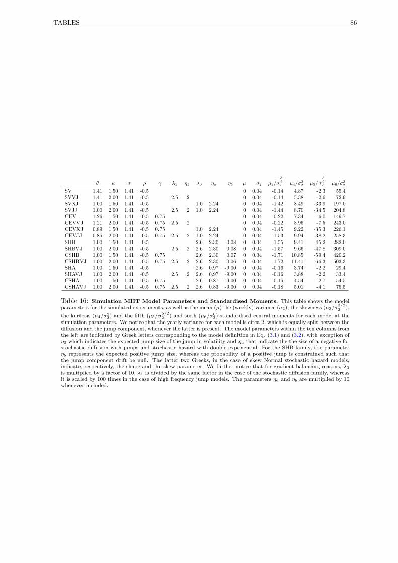
TABLES 86
θ κ σ ρ γ λ1 η1 λ0 ηa ηb µ σ2 µ3/σ322 µ4/σ
22 µ5/σ
522 µ6/σ
32
SV 1.41 1.50 1.41 -0.5 0 0.04 -0.14 4.87 -2.3 55.4SVVJ 1.41 2.00 1.41 -0.5 2.5 2 0 0.04 -0.14 5.38 -2.6 72.9SVXJ 1.00 1.50 1.41 -0.5 1.0 2.24 0 0.04 -1.42 8.49 -33.9 197.0SVJJ 1.00 2.00 1.41 -0.5 2.5 2 1.0 2.24 0 0.04 -1.44 8.70 -34.5 204.8CEV 1.26 1.50 1.41 -0.5 0.75 0 0.04 -0.22 7.34 -6.0 149.7CEVVJ 1.21 2.00 1.41 -0.5 0.75 2.5 2 0 0.04 -0.22 8.96 -7.5 243.0CEVXJ 0.89 1.50 1.41 -0.5 0.75 1.0 2.24 0 0.04 -1.45 9.22 -35.3 226.1CEVJJ 0.85 2.00 1.41 -0.5 0.75 2.5 2 1.0 2.24 0 0.04 -1.53 9.94 -38.2 258.3SHB 1.00 1.50 1.41 -0.5 2.6 2.30 0.08 0 0.04 -1.55 9.41 -45.2 282.0SHBVJ 1.00 2.00 1.41 -0.5 2.5 2 2.6 2.30 0.08 0 0.04 -1.57 9.66 -47.8 309.0CSHB 1.00 1.50 1.41 -0.5 0.75 2.6 2.30 0.07 0 0.04 -1.71 10.85 -59.4 420.2CSHBVJ 1.00 2.00 1.41 -0.5 0.75 2.5 2 2.6 2.30 0.06 0 0.04 -1.72 11.41 -66.3 503.3SHA 1.00 1.50 1.41 -0.5 2.6 0.97 -9.00 0 0.04 -0.16 3.74 -2.2 29.4SHAVJ 1.00 2.00 1.41 -0.5 2.5 2 2.6 0.97 -9.00 0 0.04 -0.16 3.88 -2.2 33.4CSHA 1.00 1.50 1.41 -0.5 0.75 2.6 0.87 -9.00 0 0.04 -0.15 4.54 -2.7 54.5CSHAVJ 1.00 2.00 1.41 -0.5 0.75 2.5 2 2.6 0.83 -9.00 0 0.04 -0.18 5.01 -4.1 75.5
Table 16: Simulation MHT Model Parameters and Standardised Moments. This table shows the modelparameters for the simulated experiments, as well as the mean (µ) the (weekly) variance (σ2), the skewness (µ3/σ
3/22 ),
the kurtosis (µ4/σ22) and the fifth (µ5/σ
5/22 ) and sixth (µ6/σ6
2) standardised central moments for each model at thesimulation parameters. We notice that the yearly variance for each model is circa 2, which is equally split between thediffusion and the jump component, whenever the latter is present. The model parameters within the ten columns fromthe left are indicated by Greek letters corresponding to the model definition in Eq. (3.1) and (3.2), with exception ofη0 which indicates the expected jump size of the jump in volatility and ηa that indicate the the size of a negative forstochastic diffusion with jumps and stochastic hazard with double exponential. For the SHB family, the parameterηb represents the expected positive jump size, whereas the probability of a positive jump is constrained such thatthe jump component drift be null. The latter two Greeks, in the case of skew Normal stochastic hazard models,indicate, respectively, the shape and the skew parameter. We further notice that for gradient balancing reasons, λ0
is multiplied by a factor of 10, λ1 is divided by the same factor in the case of the stochastic diffusion family, whereasit is scaled by 100 times in the case of high frequency jump models. The parameters ηa and ηb are multiplied by 10whenever included.

87 CHAPTER 3. MODEL SELECTION OF JUMP-DIFFUSION MODELS
θ κ σ ρ γ λ1 η1 λ0 ηa ηb
SV 1.3929 7.0560 3.7566 -0.6003(0.0052) (3.5075) (1.0017) (0.1903)
SVVJ 1.4342 8.0792 3.6425 -0.5544 2.5682 4.0251(0.0115) (3.6301) (0.7258) (0.2765) (0.3023) (0.2326)
SVXJ 1.3831 7.0447 3.7536 -0.1404 2.2707 3.0109(0.0137) (2.4441) (0.7613) (0.1618) (0.8135) (0.5025)
SVJJ 1.4032 8.0713 3.6353 -0.1123 2.5713 4.0278 2.2897 3.0088(0.0135) (3.5364) (1.1282) (0.1244) (0.3797) (0.5130) (0.1440) (0.0604)
CEV 1.3872 7.2392 3.3622 -0.4583 0.6113(0.0086) (2.7717) (0.6109) (0.1770) (0.0041)
CEVVJ 1.3978 8.2314 2.7311 -0.5000 0.6605 2.5183 4.9184(0.0066) (2.6390) (0.2126) (0.1536) (0.0046) (0.1955) (0.5727)
CEVXJ 1.3661 7.1791 3.6354 -0.1956 0.5517 2.0417 2.9293(0.0359) (2.8231) (0.8556) (0.1792) (0.0111) (0.2223) (0.2285)
CEVJJ 1.3973 8.1534 2.9306 -0.2388 0.5817 2.8949 4.4266 2.1760 3.0521(0.0093) (3.4842) (0.1000) (0.1301) (0.0120) (0.1713) (0.3350) (0.1187) (0.4411)
SHB 0.9273 7.1993 3.1988 -0.4891 1.5079 0.8520 0.7691(0.0157) (2.4277) (0.1417) (0.1773) (0.0899) (0.0114) (0.0114)
SHBVJ 0.9289 8.1939 3.2029 -0.4043 2.4959 3.9904 1.6124 0.8474 0.7631(0.0213) (4.2880) (0.9970) (0.2489) (0.2152) (0.3519) (0.5041) (0.0813) (0.2090)
CSHB 0.9262 7.2023 3.1690 -0.4735 0.4615 1.5193 0.8582 0.7714(0.0246) (2.8224) (0.4908) (0.2921) (0.0124) (0.0568) (0.0217) (0.0187)
CSHBVJ 0.9251 8.1969 3.1353 -0.4107 0.4531 2.4305 3.8970 1.6269 0.8513 0.7628(0.0158) (2.3032) (0.5645) (0.2096) (0.0029) (0.9021) (0.5776) (0.0671) (0.0079) (0.0077)
SHA 0.9102 7.0201 3.7470 -0.5595 0.9044 1.4244 -0.3356(0.0075) (3.1592) (0.8669) (0.2443) (0.0374) (0.0166) (0.0450)
SHAVJ 0.8065 8.1383 3.8650 -0.8992 2.1367 3.1327 1.5397 1.1078 -0.2333(0.0082) (3.6899) (0.5718) (0.3695) (0.7451) (0.3872) (0.0101) (0.0092) (0.0125)
CSHA 0.7765 7.1372 3.3321 -0.5445 0.8795 2.8252 0.7296 -0.4587(0.0104) (2.6834) (0.7027) (0.2113) (0.0194) (0.4307) (0.0723) (0.1548)
CSHAVJ 0.7276 8.3488 2.1948 -0.6106 0.9000 2.6211 4.1696 2.9964 0.8264 -0.5342(0.0054) (1.4450) (0.7062) (0.1619) (0.0108) (0.2016) (0.1599) (0.0374) (0.0044) (0.0122)
Table 17: Financial Market Data Model Parameters Estimates and MCS Test Results. This table showsthe parameter estimates for the Model Set, applied to the Standard & Poor’s 500 Equity Index daily log return data,ranging from January, 3rd 1950 to February, 26th 2016. Several parameters are scaled, that is θ is divided by 10while λ1 is multiplied by 10. As in the simulation test, the λ0 parameter for the stochastic hazard models is dividedby 100. In parentheses we exhibit the estimated parameter standard errors.
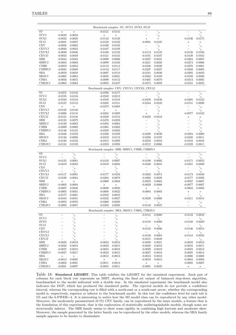
TABLES 88
Benchmark samples: SV, SVVJ, SVXJ, SVJJSV ? ? -0.0121 0.0145 − − SVVJ -0.0049 0.0053 ? ? − − SVXJ -0.0032 0.0038 -0.0142 0.0129 ? ? -0.0136 0.0175SVJJ -0.0031 0.0037 -0.0120 0.0132 -0.0091 0.0105 ? ?CEV -0.0056 0.0062 -0.0106 0.0133 − − CEVVJ -0.0026 0.0034 -0.0107 0.0129 − − CEVXJ -0.0030 0.0036 -0.0100 0.0128 -0.0113 0.0122 -0.0138 0.0180CEVJJ -0.0043 0.0049 -0.0121 0.0145 -0.0101 0.0107 -0.0139 0.0164SHB -0.0044 0.0043 -0.0099 0.0096 -0.0237 0.0031 -0.0264 0.0007SHBVJ -0.0084 0.0083 -0.0099 0.0103 -0.0241 0.0028 -0.0274 0.0006CSHB -0.0052 0.0053 -0.0112 0.0114 -0.0426 0.0039 -0.0276 0.0001CSHBVJ -0.0045 0.0048 -0.0116 0.0117 -0.0237 0.0027 -0.0269 0.0005SHA -0.0059 0.0058 -0.0097 0.0110 -0.0181 0.0030 -0.0205 0.0033SHAVJ -0.0065 0.0064 -0.0035 0.0031 -0.0562 0.0169 -0.0189 0.0026CSHA -0.0056 0.0055 -0.0099 0.0112 -0.0405 0.0070 -0.0213 0.0065CSHAVJ -0.0063 0.0063 -0.0094 0.0107 -0.0374 0.0089 -0.0161 0.0035
Benchmark samples: CEV, CEVVJ, CEVXJ, CEVJJSV -0.0255 0.0132 -0.0596 0.0177 − − SVVJ -0.0195 0.0124 -0.0582 0.0212 − − SVXJ -0.0240 0.0143 -0.0548 0.0158 -0.0250 0.0240 -0.0205 0.0122SVJJ -0.0187 0.0118 -0.0495 0.0151 -0.0244 0.0243 -0.0151 0.0096CEV ? ? -0.0273 0.0288 − − CEVVJ -0.0125 0.0140 ? ? − − CEVXJ -0.0096 0.0116 -0.0284 0.0289 ? ? -0.0077 0.0102CEVJJ -0.0121 0.0148 -0.0239 0.0154 -0.0232 0.0244 ? ?SHB -0.0132 0.0079 -0.0476 0.0228 − − SHBVJ -0.0130 0.0082 -0.0294 0.0084 − − CSHB -0.0099 0.0069 -0.0365 0.0262 − − CSHBVJ -0.0146 0.0125 -0.0359 0.0263 − − SHA -0.0166 0.0103 -0.0426 0.0199 -0.0220 0.0039 -0.0294 0.0008SHAVJ -0.0140 0.0098 -0.0319 0.0112 -0.0330 0.0197 -0.0248 0.0011CSHA -0.0126 0.0123 -0.0315 0.0280 -0.0258 0.0052 -0.0183 0.0010CSHAVJ -0.0134 0.0139 -0.0323 0.0298 -0.0212 0.0066 -0.0189 0.0011
Benchmark samples: SHB, SHBVJ, CSHB, CSHBVJSV − − − − SVVJ − − − − SVXJ -0.0132 0.0081 -0.0150 0.0097 -0.0190 0.0092 -0.0171 0.0052SVJJ -0.0219 0.0052 -0.0219 0.0056 -0.0246 0.0055 -0.0221 0.0009CEV − − − − CEVVJ − − − − CEVXJ -0.0117 0.0081 -0.0177 0.0103 -0.0202 0.0074 -0.0173 0.0040CEVJJ -0.0198 0.0084 -0.0204 0.0078 -0.0260 0.0038 -0.0177 0.0026SHB ? ? -0.0009 0.0004 -0.0023 0.0004 -0.0027 0.0007SHBVJ -0.0003 0.0004 ? ? -0.0020 0.0006 -0.0077 0.0007CSHB -0.0007 0.0026 -0.0009 0.0020 ? ? -0.0004 0.0003CSHBVJ -0.0005 0.0031 -0.0008 0.0022 -0.0004 0.0003 ? ?SHA -0.0177 0.0061 -0.0222 0.0052 − − SHAVJ -0.0164 0.0041 -0.0232 0.0027 -0.0229 0.0006 -0.0211 0.0014CSHA -0.0055 0.0076 -0.0266 0.0030 − − CSHAVJ -0.0093 0.0087 -0.0203 0.0028 -0.0143 0.0027 −
Benchmark samples: SHA, SHAVJ, CSHA, CSHAVJSV − − -0.0141 0.0000 -0.0143 0.0016SVVJ − − − − SVXJ − − -0.0158 0.0000 -0.0138 0.0029SVJJ − − − − CEV − − -0.0122 0.0006 -0.0146 0.0014CEVVJ − − − − CEVXJ − − -0.0130 0.0004 -0.0144 0.0016CEVJJ − − -0.0215 0.0038 − SHB -0.0028 0.0019 -0.0024 0.0018 -0.0029 0.0021 -0.0023 0.0013SHBVJ -0.0028 0.0018 -0.0023 0.0015 -0.0028 0.0018 -0.0016 0.0011CSHB -0.0027 0.0018 -0.0024 0.0018 -0.0029 0.0019 -0.0022 0.0013CSHBVJ -0.0027 0.0017 -0.0022 0.0015 -0.0027 0.0018 -0.0035 0.0014SHA ? ? -0.0013 0.0013 -0.0013 0.0010 -0.0006 0.0008SHAVJ -0.0013 0.0005 ? ? -0.0019 0.0012 -0.0004 0.0008CSHA -0.0002 0.0001 -0.0011 0.0012 ? ? -0.0005 0.0007CSHAVJ -0.0081 0.0007 -0.0045 0.0011 -0.0091 0.0025 ? ?
Table 18: Simulated LRMHT. This table exhibits the LRMHT for the simulated experiment. Each pair ofcolumns for each block row represents an MHT, showing the final set output of balanced step-down algorithm,benchmarked to the model indicated with a double star. In the simulated experiment the benchmark model alsoindicates the DGP, which has produced the simulated paths. The rejected models do not provide a confidenceinterval, whereas the corresponding row is filled with a north-east or a south-east arrow, whether the correspondingmodel is, respectively, superior or inferior to the benchmark model. In this test the confidence level for each tail is5% and the k-FWER=4. It is interesting to notice how the SD model class can be reproduced by any other model.Moreover, the moderately parametrised (0.75) CEV family, can be reproduced by the inner models, a feature that isthe foundation of this experiment, that is the exploration of statistically undistinguishable models, though some arestructurally inferior. The SHB family seems to show some rigidity in combining high kurtosis and moderate skew.Moreover, the sample generated by the latter family can be reproduced by the other models, whereas the SHA familysample appears to be harder to dissimulate.
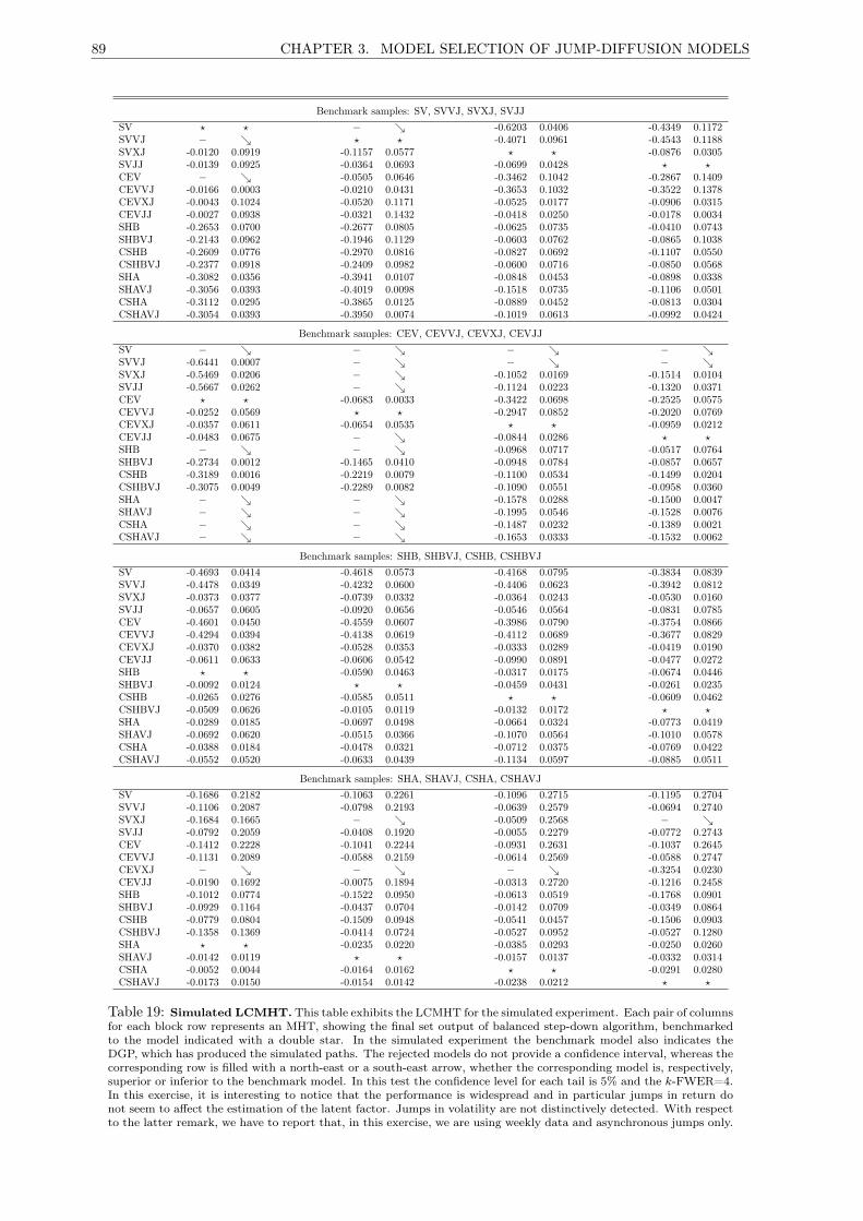
89 CHAPTER 3. MODEL SELECTION OF JUMP-DIFFUSION MODELS
Benchmark samples: SV, SVVJ, SVXJ, SVJJSV ? ? − -0.6203 0.0406 -0.4349 0.1172SVVJ − ? ? -0.4071 0.0961 -0.4543 0.1188SVXJ -0.0120 0.0919 -0.1157 0.0577 ? ? -0.0876 0.0305SVJJ -0.0139 0.0925 -0.0364 0.0693 -0.0699 0.0428 ? ?CEV − -0.0505 0.0646 -0.3462 0.1042 -0.2867 0.1409CEVVJ -0.0166 0.0003 -0.0210 0.0431 -0.3653 0.1032 -0.3522 0.1378CEVXJ -0.0043 0.1024 -0.0520 0.1171 -0.0525 0.0177 -0.0906 0.0315CEVJJ -0.0027 0.0938 -0.0321 0.1432 -0.0418 0.0250 -0.0178 0.0034SHB -0.2653 0.0700 -0.2677 0.0805 -0.0625 0.0735 -0.0410 0.0743SHBVJ -0.2143 0.0962 -0.1946 0.1129 -0.0603 0.0762 -0.0865 0.1038CSHB -0.2609 0.0776 -0.2970 0.0816 -0.0827 0.0692 -0.1107 0.0550CSHBVJ -0.2377 0.0918 -0.2409 0.0982 -0.0600 0.0716 -0.0850 0.0568SHA -0.3082 0.0356 -0.3941 0.0107 -0.0848 0.0453 -0.0898 0.0338SHAVJ -0.3056 0.0393 -0.4019 0.0098 -0.1518 0.0735 -0.1106 0.0501CSHA -0.3112 0.0295 -0.3865 0.0125 -0.0889 0.0452 -0.0813 0.0304CSHAVJ -0.3054 0.0393 -0.3950 0.0074 -0.1019 0.0613 -0.0992 0.0424
Benchmark samples: CEV, CEVVJ, CEVXJ, CEVJJSV − − − − SVVJ -0.6441 0.0007 − − − SVXJ -0.5469 0.0206 − -0.1052 0.0169 -0.1514 0.0104SVJJ -0.5667 0.0262 − -0.1124 0.0223 -0.1320 0.0371CEV ? ? -0.0683 0.0033 -0.3422 0.0698 -0.2525 0.0575CEVVJ -0.0252 0.0569 ? ? -0.2947 0.0852 -0.2020 0.0769CEVXJ -0.0357 0.0611 -0.0654 0.0535 ? ? -0.0959 0.0212CEVJJ -0.0483 0.0675 − -0.0844 0.0286 ? ?SHB − − -0.0968 0.0717 -0.0517 0.0764SHBVJ -0.2734 0.0012 -0.1465 0.0410 -0.0948 0.0784 -0.0857 0.0657CSHB -0.3189 0.0016 -0.2219 0.0079 -0.1100 0.0534 -0.1499 0.0204CSHBVJ -0.3075 0.0049 -0.2289 0.0082 -0.1090 0.0551 -0.0958 0.0360SHA − − -0.1578 0.0288 -0.1500 0.0047SHAVJ − − -0.1995 0.0546 -0.1528 0.0076CSHA − − -0.1487 0.0232 -0.1389 0.0021CSHAVJ − − -0.1653 0.0333 -0.1532 0.0062
Benchmark samples: SHB, SHBVJ, CSHB, CSHBVJSV -0.4693 0.0414 -0.4618 0.0573 -0.4168 0.0795 -0.3834 0.0839SVVJ -0.4478 0.0349 -0.4232 0.0600 -0.4406 0.0623 -0.3942 0.0812SVXJ -0.0373 0.0377 -0.0739 0.0332 -0.0364 0.0243 -0.0530 0.0160SVJJ -0.0657 0.0605 -0.0920 0.0656 -0.0546 0.0564 -0.0831 0.0785CEV -0.4601 0.0450 -0.4559 0.0607 -0.3986 0.0790 -0.3754 0.0866CEVVJ -0.4294 0.0394 -0.4138 0.0619 -0.4112 0.0689 -0.3677 0.0829CEVXJ -0.0370 0.0382 -0.0528 0.0353 -0.0333 0.0289 -0.0419 0.0190CEVJJ -0.0611 0.0633 -0.0606 0.0542 -0.0990 0.0891 -0.0477 0.0272SHB ? ? -0.0590 0.0463 -0.0317 0.0175 -0.0674 0.0446SHBVJ -0.0092 0.0124 ? ? -0.0459 0.0431 -0.0261 0.0235CSHB -0.0265 0.0276 -0.0585 0.0511 ? ? -0.0609 0.0462CSHBVJ -0.0509 0.0626 -0.0105 0.0119 -0.0132 0.0172 ? ?SHA -0.0289 0.0185 -0.0697 0.0498 -0.0664 0.0324 -0.0773 0.0419SHAVJ -0.0692 0.0620 -0.0515 0.0366 -0.1070 0.0564 -0.1010 0.0578CSHA -0.0388 0.0184 -0.0478 0.0321 -0.0712 0.0375 -0.0769 0.0422CSHAVJ -0.0552 0.0520 -0.0633 0.0439 -0.1134 0.0597 -0.0885 0.0511
Benchmark samples: SHA, SHAVJ, CSHA, CSHAVJSV -0.1686 0.2182 -0.1063 0.2261 -0.1096 0.2715 -0.1195 0.2704SVVJ -0.1106 0.2087 -0.0798 0.2193 -0.0639 0.2579 -0.0694 0.2740SVXJ -0.1684 0.1665 − -0.0509 0.2568 − SVJJ -0.0792 0.2059 -0.0408 0.1920 -0.0055 0.2279 -0.0772 0.2743CEV -0.1412 0.2228 -0.1041 0.2244 -0.0931 0.2631 -0.1037 0.2645CEVVJ -0.1131 0.2089 -0.0588 0.2159 -0.0614 0.2569 -0.0588 0.2747CEVXJ − − − -0.3254 0.0230CEVJJ -0.0190 0.1692 -0.0075 0.1894 -0.0313 0.2720 -0.1216 0.2458SHB -0.1012 0.0774 -0.1522 0.0950 -0.0613 0.0519 -0.1768 0.0901SHBVJ -0.0929 0.1164 -0.0437 0.0704 -0.0142 0.0709 -0.0349 0.0864CSHB -0.0779 0.0804 -0.1509 0.0948 -0.0541 0.0457 -0.1506 0.0903CSHBVJ -0.1358 0.1369 -0.0414 0.0724 -0.0527 0.0952 -0.0527 0.1280SHA ? ? -0.0235 0.0220 -0.0385 0.0293 -0.0250 0.0260SHAVJ -0.0142 0.0119 ? ? -0.0157 0.0137 -0.0332 0.0314CSHA -0.0052 0.0044 -0.0164 0.0162 ? ? -0.0291 0.0280CSHAVJ -0.0173 0.0150 -0.0154 0.0142 -0.0238 0.0212 ? ?
Table 19: Simulated LCMHT. This table exhibits the LCMHT for the simulated experiment. Each pair of columnsfor each block row represents an MHT, showing the final set output of balanced step-down algorithm, benchmarkedto the model indicated with a double star. In the simulated experiment the benchmark model also indicates theDGP, which has produced the simulated paths. The rejected models do not provide a confidence interval, whereas thecorresponding row is filled with a north-east or a south-east arrow, whether the corresponding model is, respectively,superior or inferior to the benchmark model. In this test the confidence level for each tail is 5% and the k-FWER=4.In this exercise, it is interesting to notice that the performance is widespread and in particular jumps in return donot seem to affect the estimation of the latent factor. Jumps in volatility are not distinctively detected. With respectto the latter remark, we have to report that, in this exercise, we are using weekly data and asynchronous jumps only.
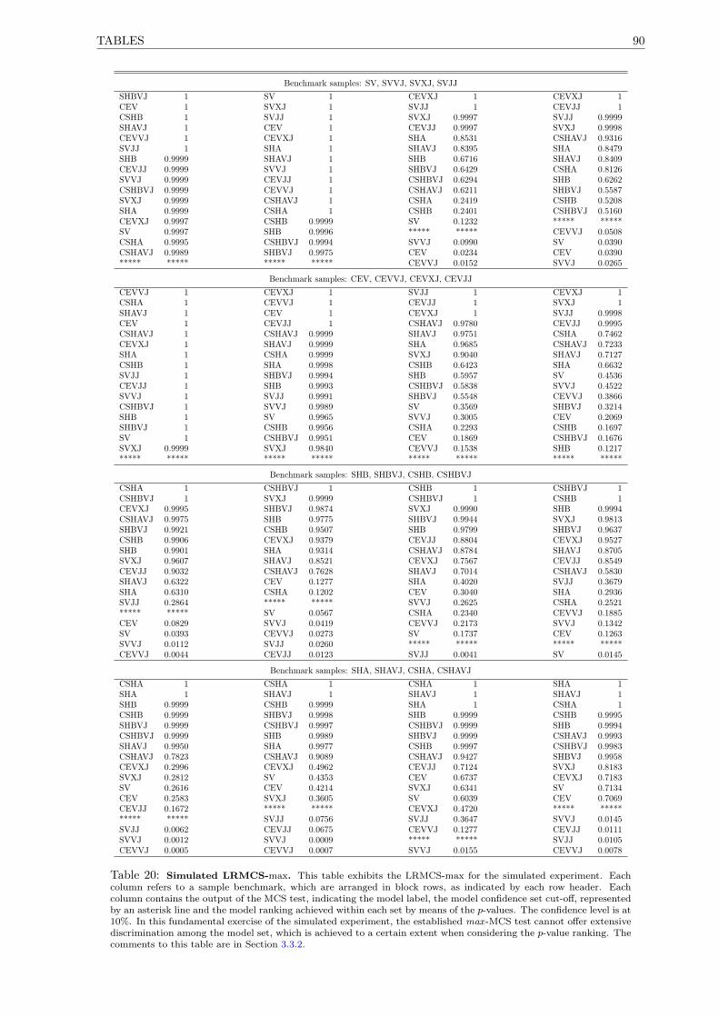
TABLES 90
Benchmark samples: SV, SVVJ, SVXJ, SVJJSHBVJ 1 SV 1 CEVXJ 1 CEVXJ 1CEV 1 SVXJ 1 SVJJ 1 CEVJJ 1CSHB 1 SVJJ 1 SVXJ 0.9997 SVJJ 0.9999SHAVJ 1 CEV 1 CEVJJ 0.9997 SVXJ 0.9998CEVVJ 1 CEVXJ 1 SHA 0.8531 CSHAVJ 0.9316SVJJ 1 SHA 1 SHAVJ 0.8395 SHA 0.8479SHB 0.9999 SHAVJ 1 SHB 0.6716 SHAVJ 0.8409CEVJJ 0.9999 SVVJ 1 SHBVJ 0.6429 CSHA 0.8126SVVJ 0.9999 CEVJJ 1 CSHBVJ 0.6294 SHB 0.6262CSHBVJ 0.9999 CEVVJ 1 CSHAVJ 0.6211 SHBVJ 0.5587SVXJ 0.9999 CSHAVJ 1 CSHA 0.2419 CSHB 0.5208SHA 0.9999 CSHA 1 CSHB 0.2401 CSHBVJ 0.5160CEVXJ 0.9997 CSHB 0.9999 SV 0.1232 ***** *****SV 0.9997 SHB 0.9996 ***** ***** CEVVJ 0.0508CSHA 0.9995 CSHBVJ 0.9994 SVVJ 0.0990 SV 0.0390CSHAVJ 0.9989 SHBVJ 0.9975 CEV 0.0234 CEV 0.0390***** ***** ***** ***** CEVVJ 0.0152 SVVJ 0.0265
Benchmark samples: CEV, CEVVJ, CEVXJ, CEVJJCEVVJ 1 CEVXJ 1 SVJJ 1 CEVXJ 1CSHA 1 CEVVJ 1 CEVJJ 1 SVXJ 1SHAVJ 1 CEV 1 CEVXJ 1 SVJJ 0.9998CEV 1 CEVJJ 1 CSHAVJ 0.9780 CEVJJ 0.9995CSHAVJ 1 CSHAVJ 0.9999 SHAVJ 0.9751 CSHA 0.7462CEVXJ 1 SHAVJ 0.9999 SHA 0.9685 CSHAVJ 0.7233SHA 1 CSHA 0.9999 SVXJ 0.9040 SHAVJ 0.7127CSHB 1 SHA 0.9998 CSHB 0.6423 SHA 0.6632SVJJ 1 SHBVJ 0.9994 SHB 0.5957 SV 0.4536CEVJJ 1 SHB 0.9993 CSHBVJ 0.5838 SVVJ 0.4522SVVJ 1 SVJJ 0.9991 SHBVJ 0.5548 CEVVJ 0.3866CSHBVJ 1 SVVJ 0.9989 SV 0.3569 SHBVJ 0.3214SHB 1 SV 0.9965 SVVJ 0.3005 CEV 0.2069SHBVJ 1 CSHB 0.9956 CSHA 0.2293 CSHB 0.1697SV 1 CSHBVJ 0.9951 CEV 0.1869 CSHBVJ 0.1676SVXJ 0.9999 SVXJ 0.9840 CEVVJ 0.1538 SHB 0.1217***** ***** ***** ***** ***** ***** ***** *****
Benchmark samples: SHB, SHBVJ, CSHB, CSHBVJCSHA 1 CSHBVJ 1 CSHB 1 CSHBVJ 1CSHBVJ 1 SVXJ 0.9999 CSHBVJ 1 CSHB 1CEVXJ 0.9995 SHBVJ 0.9874 SVXJ 0.9990 SHB 0.9994CSHAVJ 0.9975 SHB 0.9775 SHBVJ 0.9944 SVXJ 0.9813SHBVJ 0.9921 CSHB 0.9507 SHB 0.9799 SHBVJ 0.9637CSHB 0.9906 CEVXJ 0.9379 CEVJJ 0.8804 CEVXJ 0.9527SHB 0.9901 SHA 0.9314 CSHAVJ 0.8784 SHAVJ 0.8705SVXJ 0.9607 SHAVJ 0.8521 CEVXJ 0.7567 CEVJJ 0.8549CEVJJ 0.9032 CSHAVJ 0.7628 SHAVJ 0.7014 CSHAVJ 0.5830SHAVJ 0.6322 CEV 0.1277 SHA 0.4020 SVJJ 0.3679SHA 0.6310 CSHA 0.1202 CEV 0.3040 SHA 0.2936SVJJ 0.2864 ***** ***** SVVJ 0.2625 CSHA 0.2521***** ***** SV 0.0567 CSHA 0.2340 CEVVJ 0.1885CEV 0.0829 SVVJ 0.0419 CEVVJ 0.2173 SVVJ 0.1342SV 0.0393 CEVVJ 0.0273 SV 0.1737 CEV 0.1263SVVJ 0.0112 SVJJ 0.0260 ***** ***** ***** *****CEVVJ 0.0044 CEVJJ 0.0123 SVJJ 0.0041 SV 0.0145
Benchmark samples: SHA, SHAVJ, CSHA, CSHAVJCSHA 1 CSHA 1 CSHA 1 SHA 1SHA 1 SHAVJ 1 SHAVJ 1 SHAVJ 1SHB 0.9999 CSHB 0.9999 SHA 1 CSHA 1CSHB 0.9999 SHBVJ 0.9998 SHB 0.9999 CSHB 0.9995SHBVJ 0.9999 CSHBVJ 0.9997 CSHBVJ 0.9999 SHB 0.9994CSHBVJ 0.9999 SHB 0.9989 SHBVJ 0.9999 CSHAVJ 0.9993SHAVJ 0.9950 SHA 0.9977 CSHB 0.9997 CSHBVJ 0.9983CSHAVJ 0.7823 CSHAVJ 0.9089 CSHAVJ 0.9427 SHBVJ 0.9958CEVXJ 0.2996 CEVXJ 0.4962 CEVJJ 0.7124 SVXJ 0.8183SVXJ 0.2812 SV 0.4353 CEV 0.6737 CEVXJ 0.7183SV 0.2616 CEV 0.4214 SVXJ 0.6341 SV 0.7134CEV 0.2583 SVXJ 0.3605 SV 0.6039 CEV 0.7069CEVJJ 0.1672 ***** ***** CEVXJ 0.4720 ***** ********** ***** SVJJ 0.0756 SVJJ 0.3647 SVVJ 0.0145SVJJ 0.0062 CEVJJ 0.0675 CEVVJ 0.1277 CEVJJ 0.0111SVVJ 0.0012 SVVJ 0.0009 ***** ***** SVJJ 0.0105CEVVJ 0.0005 CEVVJ 0.0007 SVVJ 0.0155 CEVVJ 0.0078
Table 20: Simulated LRMCS-max. This table exhibits the LRMCS-max for the simulated experiment. Eachcolumn refers to a sample benchmark, which are arranged in block rows, as indicated by each row header. Eachcolumn contains the output of the MCS test, indicating the model label, the model confidence set cut-off, representedby an asterisk line and the model ranking achieved within each set by means of the p-values. The confidence level is at10%. In this fundamental exercise of the simulated experiment, the established max -MCS test cannot offer extensivediscrimination among the model set, which is achieved to a certain extent when considering the p-value ranking. Thecomments to this table are in Section 3.3.2.
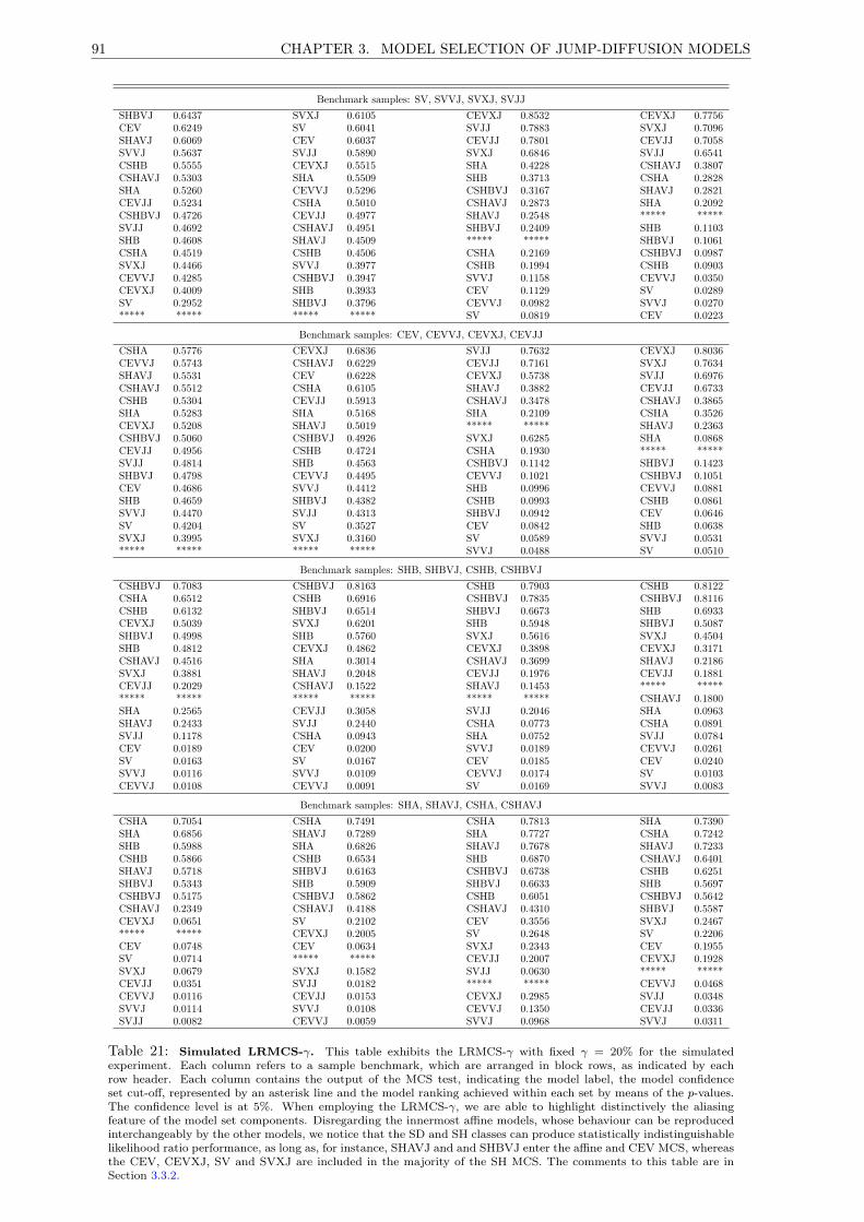
91 CHAPTER 3. MODEL SELECTION OF JUMP-DIFFUSION MODELS
Benchmark samples: SV, SVVJ, SVXJ, SVJJSHBVJ 0.6437 SVXJ 0.6105 CEVXJ 0.8532 CEVXJ 0.7756CEV 0.6249 SV 0.6041 SVJJ 0.7883 SVXJ 0.7096SHAVJ 0.6069 CEV 0.6037 CEVJJ 0.7801 CEVJJ 0.7058SVVJ 0.5637 SVJJ 0.5890 SVXJ 0.6846 SVJJ 0.6541CSHB 0.5555 CEVXJ 0.5515 SHA 0.4228 CSHAVJ 0.3807CSHAVJ 0.5303 SHA 0.5509 SHB 0.3713 CSHA 0.2828SHA 0.5260 CEVVJ 0.5296 CSHBVJ 0.3167 SHAVJ 0.2821CEVJJ 0.5234 CSHA 0.5010 CSHAVJ 0.2873 SHA 0.2092CSHBVJ 0.4726 CEVJJ 0.4977 SHAVJ 0.2548 ***** *****SVJJ 0.4692 CSHAVJ 0.4951 SHBVJ 0.2409 SHB 0.1103SHB 0.4608 SHAVJ 0.4509 ***** ***** SHBVJ 0.1061CSHA 0.4519 CSHB 0.4506 CSHA 0.2169 CSHBVJ 0.0987SVXJ 0.4466 SVVJ 0.3977 CSHB 0.1994 CSHB 0.0903CEVVJ 0.4285 CSHBVJ 0.3947 SVVJ 0.1158 CEVVJ 0.0350CEVXJ 0.4009 SHB 0.3933 CEV 0.1129 SV 0.0289SV 0.2952 SHBVJ 0.3796 CEVVJ 0.0982 SVVJ 0.0270***** ***** ***** ***** SV 0.0819 CEV 0.0223
Benchmark samples: CEV, CEVVJ, CEVXJ, CEVJJCSHA 0.5776 CEVXJ 0.6836 SVJJ 0.7632 CEVXJ 0.8036CEVVJ 0.5743 CSHAVJ 0.6229 CEVJJ 0.7161 SVXJ 0.7634SHAVJ 0.5531 CEV 0.6228 CEVXJ 0.5738 SVJJ 0.6976CSHAVJ 0.5512 CSHA 0.6105 SHAVJ 0.3882 CEVJJ 0.6733CSHB 0.5304 CEVJJ 0.5913 CSHAVJ 0.3478 CSHAVJ 0.3865SHA 0.5283 SHA 0.5168 SHA 0.2109 CSHA 0.3526CEVXJ 0.5208 SHAVJ 0.5019 ***** ***** SHAVJ 0.2363CSHBVJ 0.5060 CSHBVJ 0.4926 SVXJ 0.6285 SHA 0.0868CEVJJ 0.4956 CSHB 0.4724 CSHA 0.1930 ***** *****SVJJ 0.4814 SHB 0.4563 CSHBVJ 0.1142 SHBVJ 0.1423SHBVJ 0.4798 CEVVJ 0.4495 CEVVJ 0.1021 CSHBVJ 0.1051CEV 0.4686 SVVJ 0.4412 SHB 0.0996 CEVVJ 0.0881SHB 0.4659 SHBVJ 0.4382 CSHB 0.0993 CSHB 0.0861SVVJ 0.4470 SVJJ 0.4313 SHBVJ 0.0942 CEV 0.0646SV 0.4204 SV 0.3527 CEV 0.0842 SHB 0.0638SVXJ 0.3995 SVXJ 0.3160 SV 0.0589 SVVJ 0.0531***** ***** ***** ***** SVVJ 0.0488 SV 0.0510
Benchmark samples: SHB, SHBVJ, CSHB, CSHBVJCSHBVJ 0.7083 CSHBVJ 0.8163 CSHB 0.7903 CSHB 0.8122CSHA 0.6512 CSHB 0.6916 CSHBVJ 0.7835 CSHBVJ 0.8116CSHB 0.6132 SHBVJ 0.6514 SHBVJ 0.6673 SHB 0.6933CEVXJ 0.5039 SVXJ 0.6201 SHB 0.5948 SHBVJ 0.5087SHBVJ 0.4998 SHB 0.5760 SVXJ 0.5616 SVXJ 0.4504SHB 0.4812 CEVXJ 0.4862 CEVXJ 0.3898 CEVXJ 0.3171CSHAVJ 0.4516 SHA 0.3014 CSHAVJ 0.3699 SHAVJ 0.2186SVXJ 0.3881 SHAVJ 0.2048 CEVJJ 0.1976 CEVJJ 0.1881CEVJJ 0.2029 CSHAVJ 0.1522 SHAVJ 0.1453 ***** ********** ***** ***** ***** ***** ***** CSHAVJ 0.1800SHA 0.2565 CEVJJ 0.3058 SVJJ 0.2046 SHA 0.0963SHAVJ 0.2433 SVJJ 0.2440 CSHA 0.0773 CSHA 0.0891SVJJ 0.1178 CSHA 0.0943 SHA 0.0752 SVJJ 0.0784CEV 0.0189 CEV 0.0200 SVVJ 0.0189 CEVVJ 0.0261SV 0.0163 SV 0.0167 CEV 0.0185 CEV 0.0240SVVJ 0.0116 SVVJ 0.0109 CEVVJ 0.0174 SV 0.0103CEVVJ 0.0108 CEVVJ 0.0091 SV 0.0169 SVVJ 0.0083
Benchmark samples: SHA, SHAVJ, CSHA, CSHAVJCSHA 0.7054 CSHA 0.7491 CSHA 0.7813 SHA 0.7390SHA 0.6856 SHAVJ 0.7289 SHA 0.7727 CSHA 0.7242SHB 0.5988 SHA 0.6826 SHAVJ 0.7678 SHAVJ 0.7233CSHB 0.5866 CSHB 0.6534 SHB 0.6870 CSHAVJ 0.6401SHAVJ 0.5718 SHBVJ 0.6163 CSHBVJ 0.6738 CSHB 0.6251SHBVJ 0.5343 SHB 0.5909 SHBVJ 0.6633 SHB 0.5697CSHBVJ 0.5175 CSHBVJ 0.5862 CSHB 0.6051 CSHBVJ 0.5642CSHAVJ 0.2349 CSHAVJ 0.4188 CSHAVJ 0.4310 SHBVJ 0.5587CEVXJ 0.0651 SV 0.2102 CEV 0.3556 SVXJ 0.2467***** ***** CEVXJ 0.2005 SV 0.2648 SV 0.2206CEV 0.0748 CEV 0.0634 SVXJ 0.2343 CEV 0.1955SV 0.0714 ***** ***** CEVJJ 0.2007 CEVXJ 0.1928SVXJ 0.0679 SVXJ 0.1582 SVJJ 0.0630 ***** *****CEVJJ 0.0351 SVJJ 0.0182 ***** ***** CEVVJ 0.0468CEVVJ 0.0116 CEVJJ 0.0153 CEVXJ 0.2985 SVJJ 0.0348SVVJ 0.0114 SVVJ 0.0108 CEVVJ 0.1350 CEVJJ 0.0336SVJJ 0.0082 CEVVJ 0.0059 SVVJ 0.0968 SVVJ 0.0311
Table 21: Simulated LRMCS-γ. This table exhibits the LRMCS-γ with fixed γ = 20% for the simulatedexperiment. Each column refers to a sample benchmark, which are arranged in block rows, as indicated by eachrow header. Each column contains the output of the MCS test, indicating the model label, the model confidenceset cut-off, represented by an asterisk line and the model ranking achieved within each set by means of the p-values.The confidence level is at 5%. When employing the LRMCS-γ, we are able to highlight distinctively the aliasingfeature of the model set components. Disregarding the innermost affine models, whose behaviour can be reproducedinterchangeably by the other models, we notice that the SD and SH classes can produce statistically indistinguishablelikelihood ratio performance, as long as, for instance, SHAVJ and and SHBVJ enter the affine and CEV MCS, whereasthe CEV, CEVXJ, SV and SVXJ are included in the majority of the SH MCS. The comments to this table are inSection 3.3.2.
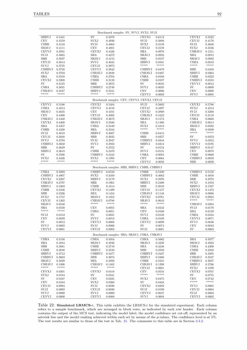
TABLES 92
Benchmark samples: SV, SVVJ, SVXJ, SVJJSHBVJ 0.5441 SV 0.5070 CEVXJ 0.6112 CEVXJ 0.5822CEV 0.4559 SVXJ 0.4930 SVJJ 0.3888 CEVJJ 0.4178CSHB 0.4134 SVJJ 0.4864 SVXJ 0.3159 SVJJ 0.3638SHAVJ 0.4111 CEV 0.4801 CEVJJ 0.3159 SVXJ 0.3166CEVVJ 0.3931 CEVXJ 0.4426 SHA 0.0978 CSHAVJ 0.1311SVJJ 0.3865 SHA 0.4272 SHAVJ 0.0932 SHA 0.0915SHB 0.3837 SHAVJ 0.4154 SHB 0.0547 SHAVJ 0.0892CEVJJ 0.3814 SVVJ 0.4045 SHBVJ 0.0501 CSHA 0.0810SVVJ 0.3735 CEVJJ 0.3972 ***** ***** ***** *****CSHBVJ 0.3728 CEVVJ 0.3942 CSHBVJ 0.0479 SHB 0.0450SVXJ 0.3703 CSHAVJ 0.3828 CSHAVJ 0.0467 SHBVJ 0.0364SHA 0.3558 CSHA 0.3704 CSHA 0.0108 CSHB 0.0323CEVXJ 0.3208 CSHB 0.3133 CSHB 0.0107 CSHBVJ 0.0318SV 0.3125 SHB 0.2855 SV 0.0045 CEVVJ 0.0014CSHA 0.3031 CSHBVJ 0.2748 SVVJ 0.0035 SV 0.0009CSHAVJ 0.2847 SHBVJ 0.2341 CEV 0.0006 CEV 0.0008***** ***** ***** ***** CEVVJ 0.0003 SVVJ 0.0005
Benchmark samples: CEV, CEVVJ, CEVXJ, CEVJJCEVVJ 0.5186 CEVXJ 0.5484 SVJJ 0.5603 CEVXJ 0.5786CSHA 0.4814 CEVVJ 0.4516 CEVJJ 0.4397 SVXJ 0.4214SHAVJ 0.4635 CEV 0.4101 CEVXJ 0.3869 SVJJ 0.3260CEV 0.4490 CEVJJ 0.4092 CSHAVJ 0.1622 CEVJJ 0.3110CSHAVJ 0.4440 CSHAVJ 0.3673 SHAVJ 0.1574 CSHA 0.0660CEVXJ 0.4408 SHAVJ 0.3586 SHA 0.1486 CSHAVJ 0.0614SHA 0.4357 CSHA 0.3449 SVXJ 0.1013 SHAVJ 0.0592CSHB 0.4338 SHA 0.3344 ***** ***** SHA 0.0509SVJJ 0.4018 SHBVJ 0.3087 CSHB 0.0415 ***** *****CEVJJ 0.3828 SHB 0.3035 SHB 0.0357 SV 0.0253SVVJ 0.3794 SVJJ 0.2947 CSHBVJ 0.0344 SVVJ 0.0252CSHBVJ 0.3650 SVVJ 0.2923 SHBVJ 0.0314 CEVVJ 0.0195SHB 0.3629 SV 0.2552 SV 0.0154 SHBVJ 0.0147SHBVJ 0.3618 CSHB 0.2470 SVVJ 0.0121 CEV 0.0078SV 0.3586 CSHBVJ 0.2416 CSHA 0.0084 CSHB 0.0060SVXJ 0.3426 SVXJ 0.1995 CEV 0.0064 CSHBVJ 0.0059***** ***** ***** ***** CEVVJ 0.0050 SHB 0.0039
Benchmark samples: SHB, SHBVJ, CSHB, CSHBVJCSHA 0.5093 CSHBVJ 0.6550 CSHB 0.5339 CSHBVJ 0.5150CSHBVJ 0.4907 SVXJ 0.3450 CSHBVJ 0.4662 CSHB 0.4850CEVXJ 0.3207 SHBVJ 0.2179 SVXJ 0.2976 SHB 0.2978CSHAVJ 0.2797 SHB 0.1961 SHBVJ 0.2490 SVXJ 0.1853SHBVJ 0.2403 CSHB 0.1614 SHB 0.2010 SHBVJ 0.1587CSHB 0.2346 CEVXJ 0.1499 CEVJJ 0.1157 CEVXJ 0.1472SHB 0.2336 SHA 0.1454 CSHAVJ 0.1148 SHAVJ 0.0986SVXJ 0.1757 SHAVJ 0.1052 CEVXJ 0.0761 CEVJJ 0.0924CEVJJ 0.1302 CSHAVJ 0.0788 SHAVJ 0.0643 ***** *****SHAVJ 0.0540 ***** ***** ***** ***** CSHAVJ 0.0384SHA 0.0538 CEV 0.0055 SHA 0.0242 SVJJ 0.0178***** ***** CSHA 0.0051 CEV 0.0160 SHA 0.0129SVJJ 0.0153 SV 0.0021 SVVJ 0.0128 CSHA 0.0104CEV 0.0029 SVVJ 0.0013 CSHA 0.0109 CEVVJ 0.0071SV 0.0012 CEVVJ 0.0008 CEVVJ 0.0099 SVVJ 0.0046SVVJ 0.0002 SVJJ 0.0006 SV 0.0074 CEV 0.0043CEVVJ 0.0001 CEVJJ 0.0003 SVJJ 0.0001 SV 0.0003
Benchmark samples: SHA, SHAVJ, CSHA, CSHAVJCSHA 0.5156 CSHA 0.5054 CSHA 0.5662 SHA 0.5077SHA 0.4844 SHAVJ 0.4946 SHAVJ 0.4338 SHAVJ 0.4923SHB 0.3881 CSHB 0.3719 SHA 0.4248 CSHA 0.4390CSHB 0.3840 SHBVJ 0.3533 SHB 0.3593 CSHB 0.3332SHBVJ 0.3712 CSHBVJ 0.3477 CSHBVJ 0.3437 SHB 0.3285CSHBVJ 0.3663 SHB 0.3074 SHBVJ 0.3406 CSHAVJ 0.3247SHAVJ 0.2829 SHA 0.2893 CSHB 0.3101 CSHBVJ 0.3037CSHAVJ 0.1006 CSHAVJ 0.1482 CSHAVJ 0.1398 SHBVJ 0.2766***** ***** ***** ***** CEVJJ 0.0601 SVXJ 0.1039CEVXJ 0.0201 CEVXJ 0.0418 CEV 0.0534 CEVXJ 0.0767SVXJ 0.0184 SV 0.0341 ***** ***** SV 0.0755SV 0.0167 CEV 0.0325 SVXJ 0.0475 CEV 0.0742CEV 0.0164 SVXJ 0.0260 SV 0.0434 ***** *****CEVJJ 0.0094 SVJJ 0.0036 CEVXJ 0.0283 SVVJ 0.0005SVJJ 0.0002 CEVJJ 0.0030 SVJJ 0.0190 CEVJJ 0.0004SVVJ 0.0000 SVVJ 0.0000 CEVVJ 0.0047 SVJJ 0.0003CEVVJ 0.0000 CEVVJ 0.0000 SVVJ 0.0004 CEVVJ 0.0002
Table 22: Simulated LRMCS-t. This table exhibits the LRMCS-t for the simulated experiment. Each columnrefers to a sample benchmark, which are arranged in block rows, as indicated by each row header. Each columncontains the output of the MCS test, indicating the model label, the model confidence set cut-off, represented by anasterisk line and the model ranking achieved within each set by means of the p-values. The confidence level is at 5%.The test results are similar to those of the test in Tab. 21. The comments to this table are in Section 3.3.2.
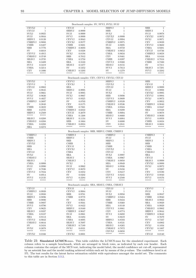
93 CHAPTER 3. MODEL SELECTION OF JUMP-DIFFUSION MODELS
Benchmark samples: SV, SVVJ, SVXJ, SVJJCEVXJ 1 CEVJJ 1 SHBVJ 1 SHB 1CEVJJ 1 SHBVJ 0.9999 SHB 1 SHBVJ 1SVXJ 0.9925 SVJJ 0.9999 SVXJ 1 SVJJ 0.9978SVJJ 0.9916 SVVJ 0.9999 CEVXJ 0.9999 CEVXJ 0.9972SHBVJ 0.9139 CEVVJ 0.9943 CEVJJ 0.9994 SVXJ 0.9971CSHBVJ 0.9088 CEVXJ 0.9577 CSHBVJ 0.9975 CEV 0.9839CSHB 0.8487 CSHB 0.9281 SVJJ 0.9895 CEVVJ 0.9602SHB 0.7776 CSHBVJ 0.8693 SHA 0.9759 CSHA 0.9281SV 0.6018 CEV 0.8338 CSHAVJ 0.9653 CEVJJ 0.8736CEVVJ 0.4915 SVXJ 0.8194 CSHA 0.9634 CSHBVJ 0.8658CSHAVJ 0.3749 SHB 0.7012 CEV 0.9461 SHA 0.8416SHAVJ 0.3735 CSHA 0.5750 CSHB 0.9397 CSHAVJ 0.7816SHA 0.3489 SHA 0.5533 CEVVJ 0.9380 CSHB 0.7330SVVJ 0.3419 SHAVJ 0.5377 SHAVJ 0.9155 SV 0.7311CSHA 0.3214 SV 0.5352 SVVJ 0.7613 SHAVJ 0.7281CEV 0.1006 CSHAVJ 0.5293 SV 0.1279 SVVJ 0.3282***** ***** ***** ***** ***** ***** ***** *****
Benchmark samples: CEV, CEVVJ, CEVXJ, CEVJJCEVXJ 1 CEVVJ 1 SHBVJ 1 SHB 1CEVVJ 1 CEVXJ 1 CEVXJ 1 CEVJJ 1CEVJJ 0.9982 SHA 1 CEVJJ 1 SHBVJ 0.9999CEV 0.9845 SHBVJ 0.9995 SVJJ 1 SVJJ 0.9998SVJJ 0.9661 SVJJ 0.9985 SVXJ 1 CEVXJ 0.9995SVXJ 0.9630 SVXJ 0.9967 SHB 0.9890 CEVVJ 0.9994SVVJ 0.4027 SVVJ 0.9325 CEVVJ 0.9809 SVXJ 0.9973CSHBVJ 0.3897 SV 0.8703 CSHBVJ 0.9539 CEV 0.9952SV 0.3848 CEV 0.8175 CSHAVJ 0.9536 CSHBVJ 0.9840CSHB 0.3822 CSHB 0.7261 CSHA 0.9504 CSHA 0.9347SHB 0.2725 CSHBVJ 0.6822 SHA 0.9299 SHA 0.9168SHBVJ 0.2569 CEVJJ 0.2079 CSHB 0.9094 SV 0.9078***** ***** CSHA 0.1268 SHAVJ 0.8660 CSHAVJ 0.9030SHAVJ 0.0288 SHAVJ 0.1134 SVVJ 0.6084 SVVJ 0.8959CSHAVJ 0.0288 SHB 0.1064 SV 0.6000 CSHB 0.8824CSHA 0.0288 CSHAVJ 0.0924 CEV 0.2841 SHAVJ 0.8684SHA 0.0272 ***** ***** ***** ***** ***** *****
Benchmark samples: SHB, SHBVJ, CSHB, CSHBVJCSHBVJ 1 CSHBVJ 1 CSHBVJ 1 CSHBVJ 1CSHB 1 SHBVJ 1 SVJJ 1 SVJJ 1SHBVJ 1 SHB 1 SHBVJ 1 SHBVJ 1CEVXJ 1 CSHB 1 SHB 1 SHB 1SHB 1 CEVJJ 1 CSHB 1 CSHB 1SHA 1 CEVXJ 1 CEVXJ 1 CSHA 1CEVJJ 1 CSHA 1 CEVJJ 1 CSHAVJ 1SVXJ 1 SHA 1 SVXJ 0.9997 SHA 1CSHAVJ 1 SHAVJ 1 CSHA 0.9967 CEVJJ 1SHAVJ 1 CSHAVJ 1 CSHAVJ 0.9958 SHAVJ 0.9999CSHA 0.9999 SVXJ 1 SHA 0.9949 CEVXJ 0.9999SVJJ 0.9990 SVJJ 0.9962 SHAVJ 0.9936 SVXJ 0.9972CEV 0.7836 CEVVJ 0.8670 SV 0.9456 SV 0.9267CEVVJ 0.7834 CEV 0.8252 CEV 0.9417 CEV 0.9190SV 0.6914 SV 0.8202 CEVVJ 0.9245 CEVVJ 0.8840SVVJ 0.2135 SVVJ 0.2284 SVVJ 0.2580 SVVJ 0.8576***** ***** ***** ***** ***** ***** ***** *****
Benchmark samples: SHA, SHAVJ, CSHA, CSHAVJCEVJJ 1 CEVJJ 1 CEVJJ 1 CEVVJ 1CSHBVJ 0.9939 CEVVJ 0.9984 SVJJ 1 SVJJ 1SVJJ 0.9938 SHB 0.9781 SVXJ 0.9950 SHB 0.9947SHBVJ 0.9896 CSHB 0.9778 CSHBVJ 0.9484 CSHB 0.9940SHB 0.9890 SV 0.9631 SHB 0.9434 SHAVJ 0.9933CSHB 0.9807 CEV 0.9561 CSHB 0.9368 SHA 0.9929SVVJ 0.9790 SVVJ 0.9422 SHA 0.9149 CSHA 0.9929CEV 0.9625 SHBVJ 0.9160 CEVVJ 0.8861 CSHAVJ 0.9902SHAVJ 0.9337 CSHBVJ 0.9047 CEV 0.8774 SHBVJ 0.9844CSHA 0.9187 SVJJ 0.8961 SVVJ 0.8692 CSHBVJ 0.9642SHA 0.9113 SHA 0.8494 SV 0.8619 SV 0.7679CEVVJ 0.9043 CSHA 0.8095 SHBVJ 0.8593 SVVJ 0.7337CSHAVJ 0.8644 SHAVJ 0.7697 CSHA 0.8531 CEV 0.6902SV 0.3434 CSHAVJ 0.7189 SHAVJ 0.8265 SVXJ 0.1856SVXJ 0.2678 SVXJ 0.0521 CSHAVJ 0.7872 CEVXJ 0.1807***** ***** ***** ***** CEVXJ 0.0658 ***** *****CEVXJ 0.0166 CEVXJ 0.0001 ***** ***** CEVJJ 0.0140
Table 23: Simulated LCMCS-max. This table exhibits the LCMCS-max for the simulated experiment. Eachcolumn refers to a sample benchmark, which are arranged in block rows, as indicated by each row header. Eachcolumn contains the output of the MCS test, indicating the model label, the model confidence set cut-off, representedby an asterisk line and the model ranking achieved within each set by means of the p-values. The confidence level is at5%. The test results for the latent factor estimation exhibit wide equivalence amongst the model set. The commentsto this table are in Section 3.3.2.

TABLES 94
Benchmark samples: SV, SVVJ, SVXJ, SVJJCEVJJ 0.9305 CEVJJ 0.8792 SHBVJ 0.7870 SHB 0.8550CEVXJ 0.9055 SVJJ 0.7426 SHB 0.7851 SHBVJ 0.7587SVXJ 0.8503 CEVXJ 0.7369 CSHBVJ 0.7402 SVJJ 0.7140SVJJ 0.8207 SHBVJ 0.7188 SVXJ 0.6775 CSHBVJ 0.6568SV 0.6475 SVVJ 0.6985 CEVJJ 0.6127 CEVJJ 0.6081CEVVJ 0.5635 CEVVJ 0.6499 CSHB 0.6114 SVXJ 0.5710SHBVJ 0.5380 CSHBVJ 0.5759 CEVXJ 0.5903 CEVXJ 0.5461SVVJ 0.4779 CEV 0.5463 SVJJ 0.5667 CSHA 0.4867CSHBVJ 0.4558 SVXJ 0.4877 SHA 0.5076 CSHB 0.4749CEV 0.4187 SHB 0.4675 CSHAVJ 0.4929 SHA 0.4574CSHB 0.3700 CSHB 0.4390 CSHA 0.4535 CSHAVJ 0.4446SHB 0.3103 CSHA 0.1813 SHAVJ 0.3732 SHAVJ 0.4054CSHAVJ 0.2345 SHA 0.1392 CEV 0.3208 CEV 0.3931SHAVJ 0.2065 SHAVJ 0.1224 CEVVJ 0.2593 CEVVJ 0.3135SHA 0.1530 CSHAVJ 0.1148 SVVJ 0.1764 SV 0.1821CSHA 0.1174 ***** ***** SV 0.0454 SVVJ 0.1326***** ***** SV 0.3563 ***** ***** ***** *****
Benchmark samples: CEV, CEVVJ, CEVXJ, CEVJJCEVXJ 0.9044 CEVVJ 0.8703 SHBVJ 0.8327 SHB 0.8596CEVJJ 0.8266 CEVXJ 0.8126 SHB 0.7748 SHBVJ 0.7702CEVVJ 0.7504 SHBVJ 0.6336 CEVXJ 0.7069 CEVJJ 0.7421CEV 0.7347 CEV 0.5808 CSHBVJ 0.6646 CSHBVJ 0.7040SVJJ 0.5177 SVJJ 0.3888 CSHB 0.5956 CEVXJ 0.6205SVXJ 0.5013 SVVJ 0.1951 CEVJJ 0.5740 SVJJ 0.5534CSHBVJ 0.3596 SV 0.0188 SVXJ 0.5069 CSHB 0.5026SHBVJ 0.3498 ***** ***** SVJJ 0.5043 CEVVJ 0.4813SVVJ 0.2548 CSHB 0.4394 CSHAVJ 0.3954 SVXJ 0.4689SHB 0.1854 CSHBVJ 0.4361 CSHA 0.3777 CSHA 0.4388SV 0.1155 SHB 0.4098 SHA 0.3634 SHAVJ 0.4094***** ***** SVXJ 0.3285 SHAVJ 0.2812 CSHAVJ 0.4025CSHB 0.3032 CSHA 0.2336 CEVVJ 0.2721 SHA 0.3951SHAVJ 0.1632 SHAVJ 0.2326 CEV 0.1507 CEV 0.3607CSHAVJ 0.1537 SHA 0.2304 ***** ***** SV 0.1637CSHA 0.1507 CSHAVJ 0.2212 SVVJ 0.0279 SVVJ 0.1272SHA 0.1422 CEVJJ 0.0139 SV 0.0263 ***** *****
Benchmark samples: SHB, SHBVJ, CSHB, CSHBVJCSHBVJ 0.6981 CSHBVJ 0.7101 CSHBVJ 0.7297 CSHBVJ 0.7446SHBVJ 0.6737 SHBVJ 0.7068 SHBVJ 0.7111 SHBVJ 0.6803CSHB 0.6503 SHB 0.6661 SVJJ 0.6889 SVJJ 0.6217CEVXJ 0.6467 CSHB 0.6466 CSHB 0.6731 SHB 0.6181SHB 0.6454 CEVXJ 0.6253 SHB 0.6551 CSHB 0.6152SVXJ 0.6321 CEVJJ 0.6091 CEVXJ 0.6536 CEVXJ 0.6089CEVJJ 0.6189 CSHA 0.5939 SVXJ 0.6160 CEVJJ 0.5984SHA 0.6037 SHA 0.5865 CEVJJ 0.5536 CSHA 0.5654CSHAVJ 0.5938 SHAVJ 0.5719 SHA 0.5088 SHA 0.5366SHAVJ 0.5570 SVXJ 0.5380 CSHA 0.5024 CSHAVJ 0.5306CSHA 0.5368 CSHAVJ 0.5319 CSHAVJ 0.4466 SVXJ 0.5281SVJJ 0.5328 SVJJ 0.5143 SHAVJ 0.4430 SHAVJ 0.4805CEVVJ 0.2281 CEVVJ 0.2652 CEV 0.2763 CEV 0.2571CEV 0.1648 SVVJ 0.1882 SV 0.2359 SV 0.2523SVVJ 0.1331 CEV 0.1549 CEVVJ 0.2165 CEVVJ 0.2347SV 0.0847 SV 0.0912 SVVJ 0.0893 SVVJ 0.1274***** ***** ***** ***** ***** ***** ***** *****
Benchmark samples: SHA, SHAVJ, CSHA, CSHAVJCEVJJ 0.8583 CEVJJ 0.8814 SVJJ 0.8554 CEVVJ 0.8261SVJJ 0.6651 CEVVJ 0.7450 CEVJJ 0.8476 SVJJ 0.7171SVVJ 0.5975 SVJJ 0.6765 CEVVJ 0.6870 SVVJ 0.7169SHBVJ 0.5588 SVVJ 0.6212 SVXJ 0.6360 CEV 0.5075CEVVJ 0.5333 CSHBVJ 0.5163 SVVJ 0.6217 SHBVJ 0.4688CSHB 0.5254 SHBVJ 0.5052 CSHBVJ 0.5189 CSHBVJ 0.4588SHB 0.5004 CEV 0.4840 SHBVJ 0.5039 SV 0.4287CSHBVJ 0.4975 SV 0.4491 CEV 0.4779 SHA 0.4145CSHA 0.4619 CSHB 0.3922 SHB 0.3994 CSHA 0.4112SHAVJ 0.4617 SHB 0.3897 SV 0.3851 SHAVJ 0.4088SHA 0.4568 SHAVJ 0.3464 CSHB 0.3651 CSHAVJ 0.4006CSHAVJ 0.4366 SHA 0.3376 CSHA 0.3160 CSHB 0.3895CEV 0.4320 CSHA 0.3329 SHAVJ 0.3066 SHB 0.3517SV 0.2861 CSHAVJ 0.3226 SHA 0.2969 ***** *****SVXJ 0.2288 ***** ***** CSHAVJ 0.2824 CEVJJ 0.4520***** ***** SVXJ 0.0150 ***** ***** CEVXJ 0.0430CEVXJ 0.0022 CEVXJ 0.0049 CEVXJ 0.0054 SVXJ 0.0202
Table 24: Simulated LCMCS-γ. This table exhibits the LCMCS-γ with γ = 10% for the simulated experiment.Each column refers to a sample benchmark, which are arranged in block rows, as indicated by each row header. Eachcolumn contains the output of the MCS test, indicating the model label, the model confidence set cut-off, representedby an asterisk line and the model ranking achieved within each set by means of the p-values. The confidence level isat 5%. Considering the k, with the exception of CEV and CSHBVJ whereby k = 2 and CEVVJ whereby k = 3, allthe model tests select k = 1. The comments to this table are in Section 3.3.2.
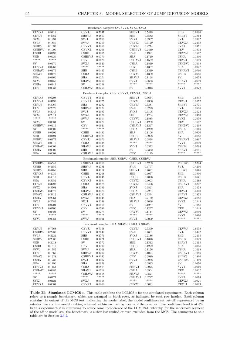
95 CHAPTER 3. MODEL SELECTION OF JUMP-DIFFUSION MODELS
Benchmark samples: SV, SVVJ, SVXJ, SVJJCEVXJ 0.5418 CEVJJ 0.7147 SHBVJ 0.5418 SHB 0.6186CEVJJ 0.4582 SHBVJ 0.2853 SHB 0.4582 SHBVJ 0.3814SVXJ 0.1894 SVJJ 0.2769 SVXJ 0.3967 SVJJ 0.2507SVJJ 0.1859 SVVJ 0.2719 CEVXJ 0.3129 CEVXJ 0.2458SHBVJ 0.1032 CEVVJ 0.1869 CEVJJ 0.2774 SVXJ 0.2451CSHBVJ 0.1009 CEVXJ 0.1206 CSHBVJ 0.2440 CEV 0.1933CSHB 0.0795 CSHB 0.1005 SVJJ 0.1991 CEVVJ 0.1567SHB 0.0629 CSHBVJ 0.0770 SHA 0.1710 CSHA 0.1300***** ***** CEV 0.0673 CSHAVJ 0.1562 CEVJJ 0.1039SV 0.0370 SVXJ 0.0640 CSHA 0.1539 CSHBVJ 0.1008CEVVJ 0.0265 ***** ***** CEV 0.1367 SHA 0.0927CSHAVJ 0.0177 SHB 0.0437 CSHB 0.1319 CSHAVJ 0.0760SHAVJ 0.0176 CSHA 0.0294 CEVVJ 0.1309 CSHB 0.0658SHA 0.0160 SHA 0.0274 SHAVJ 0.1168 SV 0.0654SVVJ 0.0156 SHAVJ 0.0260 SVVJ 0.0663 SHAVJ 0.0649CSHA 0.0143 SV 0.0258 ***** ***** ***** *****CEV 0.0033 CSHAVJ 0.0253 SV 0.0043 SVVJ 0.0172
Benchmark samples: CEV, CEVVJ, CEVXJ, CEVJJCEVXJ 0.6208 CEVVJ 0.5625 SHBVJ 0.5634 SHB 0.6848CEVVJ 0.3792 CEVXJ 0.4375 CEVXJ 0.4366 CEVJJ 0.3152CEVJJ 0.3069 SHA 0.4282 CEVJJ 0.3381 SHBVJ 0.2771CEV 0.2376 SHBVJ 0.2324 SVJJ 0.3223 SVJJ 0.2696SVJJ 0.2045 SVJJ 0.2087 SVXJ 0.3108 CEVXJ 0.2523SVXJ 0.2011 SVXJ 0.1926 SHB 0.1764 CEVVJ 0.2450***** ***** SVVJ 0.1014 CEVVJ 0.1585 SVXJ 0.2059SVVJ 0.0331 SV 0.0774 CSHBVJ 0.1269 CEV 0.1887CSHBVJ 0.0315 CEV 0.0644 CSHAVJ 0.1267 CSHBVJ 0.1499SV 0.0309 ***** ***** CSHA 0.1239 CSHA 0.1016CSHB 0.0306 CSHB 0.0483 SHA 0.1106 SHA 0.0926SHB 0.0191 CSHBVJ 0.0424 CSHB 0.0998 SV 0.0888SHBVJ 0.0177 CEVJJ 0.0070 SHAVJ 0.0838 CSHAVJ 0.0867SHAVJ 0.0010 CSHA 0.0038 ***** ***** SVVJ 0.0839CSHAVJ 0.0009 SHAVJ 0.0033 SVVJ 0.0372 CSHB 0.0794CSHA 0.0009 SHB 0.0031 SV 0.0362 SHAVJ 0.0751SHA 0.0008 CSHAVJ 0.0026 CEV 0.0115 ***** *****
Benchmark samples: SHB, SHBVJ, CSHB, CSHBVJCSHBVJ 0.5543 CSHBVJ 0.5219 CSHBVJ 0.5203 CSHBVJ 0.5704CSHB 0.4457 SHBVJ 0.4781 SVJJ 0.4797 SVJJ 0.4296SHBVJ 0.4456 SHB 0.4317 SHBVJ 0.4621 SHBVJ 0.3976CEVXJ 0.4039 CSHB 0.4268 SHB 0.4077 SHB 0.3906SHB 0.4015 CEVJJ 0.3745 CSHB 0.4026 CSHB 0.3871SHA 0.3952 CEVXJ 0.3694 CEVXJ 0.4003 CSHA 0.3289CEVJJ 0.3793 CSHA 0.3578 CEVJJ 0.3496 CSHAVJ 0.3227SVXJ 0.3768 SHA 0.3399 SVXJ 0.2861 SHA 0.3178CSHAVJ 0.3676 SHAVJ 0.3373 CSHA 0.2281 CEVJJ 0.3100SHAVJ 0.3415 CSHAVJ 0.3252 CSHAVJ 0.2224 SHAVJ 0.2872CSHA 0.2961 SVXJ 0.3045 SHA 0.2159 CEVXJ 0.2788SVJJ 0.2582 SVJJ 0.2248 SHAVJ 0.2096 SVXJ 0.2148CEV 0.0701 CEVVJ 0.0919 SV 0.1287 SV 0.1088CEVVJ 0.0700 CEV 0.0789 CEV 0.1257 CEV 0.1049SV 0.0524 SV 0.0775 CEVVJ 0.1144 CEVVJ 0.0899***** ***** ***** ***** ***** ***** SVVJ 0.0810SVVJ 0.0084 SVVJ 0.0091 SVVJ 0.0099 ***** *****
Benchmark samples: SHA, SHAVJ, CSHA, CSHAVJCEVJJ 0.7768 CEVJJ 0.7358 CEVJJ 0.5399 CEVVJ 0.6558CSHBVJ 0.2232 CEVVJ 0.2642 SVJJ 0.4601 SVJJ 0.3442SVJJ 0.2224 SHB 0.1776 SVXJ 0.2186 SHB 0.2195SHBVJ 0.2038 CSHB 0.1771 CSHBVJ 0.1376 CSHB 0.2149SHB 0.2018 SV 0.1572 SHB 0.1342 SHAVJ 0.2115CSHB 0.1816 CEV 0.1492 CSHB 0.1292 SHA 0.2098SVVJ 0.1785 SVVJ 0.1368 SHA 0.1156 CSHA 0.2098CEV 0.1565 SHBVJ 0.1202 CEVVJ 0.1024 CSHAVJ 0.1986SHAVJ 0.1328 CSHBVJ 0.1143 CEV 0.0989 SHBVJ 0.1816CSHA 0.1236 SVJJ 0.1107 SVVJ 0.0958 CSHBVJ 0.1499SHA 0.1190 SHA 0.0928 SV 0.0933 SV 0.0676CEVVJ 0.1154 CSHA 0.0814 SHBVJ 0.0925 SVVJ 0.0610CSHAVJ 0.0985 SHAVJ 0.0718 CSHA 0.0904 CEV 0.0537***** ***** CSHAVJ 0.0618 SHAVJ 0.0824 ***** *****SV 0.0177 ***** ***** CSHAVJ 0.0727 SVXJ 0.0074SVXJ 0.0124 SVXJ 0.0016 ***** ***** CEVXJ 0.0071CEVXJ 0.0004 CEVXJ 0.0000 CEVXJ 0.0021 CEVJJ 0.0003
Table 25: Simulated LCMCS-t. This table exhibits the LCMCS-t for the simulated experiment. Each columnrefers to a sample benchmark, which are arranged in block rows, as indicated by each row header. Each columncontains the output of the MCS test, indicating the model label, the model confidence set cut-off, represented by anasterisk line and the model ranking achieved within each set by means of the p-values. The confidence level is at 5%.In this experiment it is interesting to notice some incoherence of the LCMCS-t, whereby, for the innermost segmentof the affine model set, the benchmark is either low ranked or even excluded from the MCS. The comments to thistable are in Section 3.3.2.
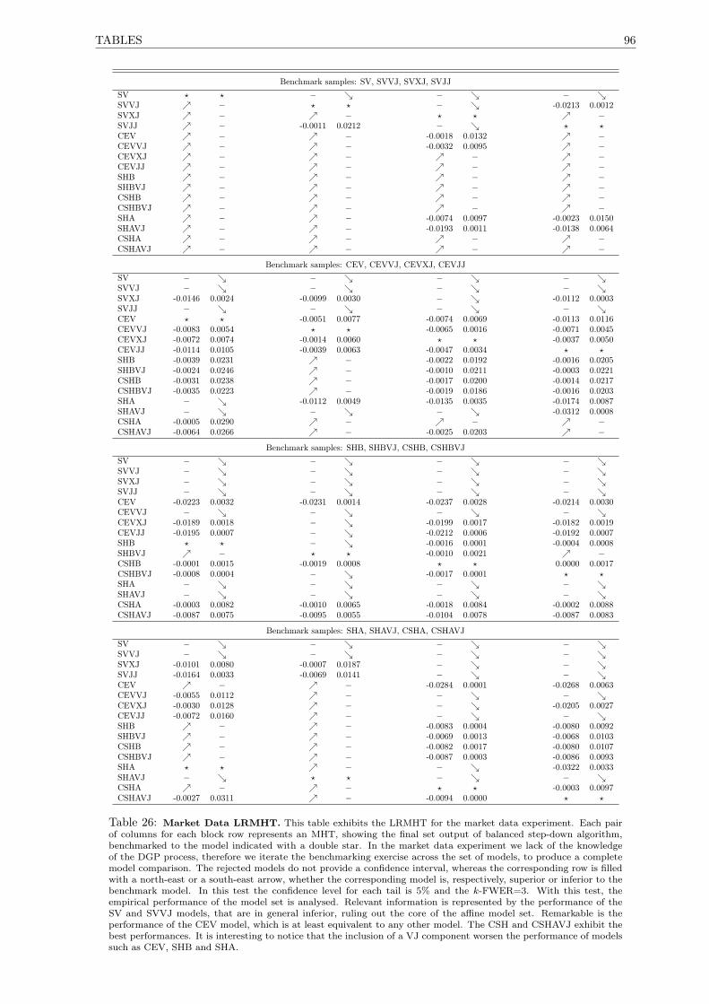
TABLES 96
Benchmark samples: SV, SVVJ, SVXJ, SVJJSV ? ? − − − SVVJ − ? ? − -0.0213 0.0012SVXJ − − ? ? −SVJJ − -0.0011 0.0212 − ? ?CEV − − -0.0018 0.0132 −CEVVJ − − -0.0032 0.0095 −CEVXJ − − − −CEVJJ − − − −SHB − − − −SHBVJ − − − −CSHB − − − −CSHBVJ − − − −SHA − − -0.0074 0.0097 -0.0023 0.0150SHAVJ − − -0.0193 0.0011 -0.0138 0.0064CSHA − − − −CSHAVJ − − − −
Benchmark samples: CEV, CEVVJ, CEVXJ, CEVJJSV − − − − SVVJ − − − − SVXJ -0.0146 0.0024 -0.0099 0.0030 − -0.0112 0.0003SVJJ − − − − CEV ? ? -0.0051 0.0077 -0.0074 0.0069 -0.0113 0.0116CEVVJ -0.0083 0.0054 ? ? -0.0065 0.0016 -0.0071 0.0045CEVXJ -0.0072 0.0074 -0.0014 0.0060 ? ? -0.0037 0.0050CEVJJ -0.0114 0.0105 -0.0039 0.0063 -0.0047 0.0034 ? ?SHB -0.0039 0.0231 − -0.0022 0.0192 -0.0016 0.0205SHBVJ -0.0024 0.0246 − -0.0010 0.0211 -0.0003 0.0221CSHB -0.0031 0.0238 − -0.0017 0.0200 -0.0014 0.0217CSHBVJ -0.0035 0.0223 − -0.0019 0.0186 -0.0016 0.0203SHA − -0.0112 0.0049 -0.0135 0.0035 -0.0174 0.0087SHAVJ − − − -0.0312 0.0008CSHA -0.0005 0.0290 − − −CSHAVJ -0.0064 0.0266 − -0.0025 0.0203 −
Benchmark samples: SHB, SHBVJ, CSHB, CSHBVJSV − − − − SVVJ − − − − SVXJ − − − − SVJJ − − − − CEV -0.0223 0.0032 -0.0231 0.0014 -0.0237 0.0028 -0.0214 0.0030CEVVJ − − − − CEVXJ -0.0189 0.0018 − -0.0199 0.0017 -0.0182 0.0019CEVJJ -0.0195 0.0007 − -0.0212 0.0006 -0.0192 0.0007SHB ? ? − -0.0016 0.0001 -0.0004 0.0008SHBVJ − ? ? -0.0010 0.0021 −CSHB -0.0001 0.0015 -0.0019 0.0008 ? ? 0.0000 0.0017CSHBVJ -0.0008 0.0004 − -0.0017 0.0001 ? ?SHA − − − − SHAVJ − − − − CSHA -0.0003 0.0082 -0.0010 0.0065 -0.0018 0.0084 -0.0002 0.0088CSHAVJ -0.0087 0.0075 -0.0095 0.0055 -0.0104 0.0078 -0.0087 0.0083
Benchmark samples: SHA, SHAVJ, CSHA, CSHAVJSV − − − − SVVJ − − − − SVXJ -0.0101 0.0080 -0.0007 0.0187 − − SVJJ -0.0164 0.0033 -0.0069 0.0141 − − CEV − − -0.0284 0.0001 -0.0268 0.0063CEVVJ -0.0055 0.0112 − − − CEVXJ -0.0030 0.0128 − − -0.0205 0.0027CEVJJ -0.0072 0.0160 − − − SHB − − -0.0083 0.0004 -0.0080 0.0092SHBVJ − − -0.0069 0.0013 -0.0068 0.0103CSHB − − -0.0082 0.0017 -0.0080 0.0107CSHBVJ − − -0.0087 0.0003 -0.0086 0.0093SHA ? ? − − -0.0322 0.0033SHAVJ − ? ? − − CSHA − − ? ? -0.0003 0.0097CSHAVJ -0.0027 0.0311 − -0.0094 0.0000 ? ?
Table 26: Market Data LRMHT. This table exhibits the LRMHT for the market data experiment. Each pairof columns for each block row represents an MHT, showing the final set output of balanced step-down algorithm,benchmarked to the model indicated with a double star. In the market data experiment we lack of the knowledgeof the DGP process, therefore we iterate the benchmarking exercise across the set of models, to produce a completemodel comparison. The rejected models do not provide a confidence interval, whereas the corresponding row is filledwith a north-east or a south-east arrow, whether the corresponding model is, respectively, superior or inferior to thebenchmark model. In this test the confidence level for each tail is 5% and the k-FWER=3. With this test, theempirical performance of the model set is analysed. Relevant information is represented by the performance of theSV and SVVJ models, that are in general inferior, ruling out the core of the affine model set. Remarkable is theperformance of the CEV model, which is at least equivalent to any other model. The CSH and CSHAVJ exhibit thebest performances. It is interesting to notice that the inclusion of a VJ component worsen the performance of modelssuch as CEV, SHB and SHA.
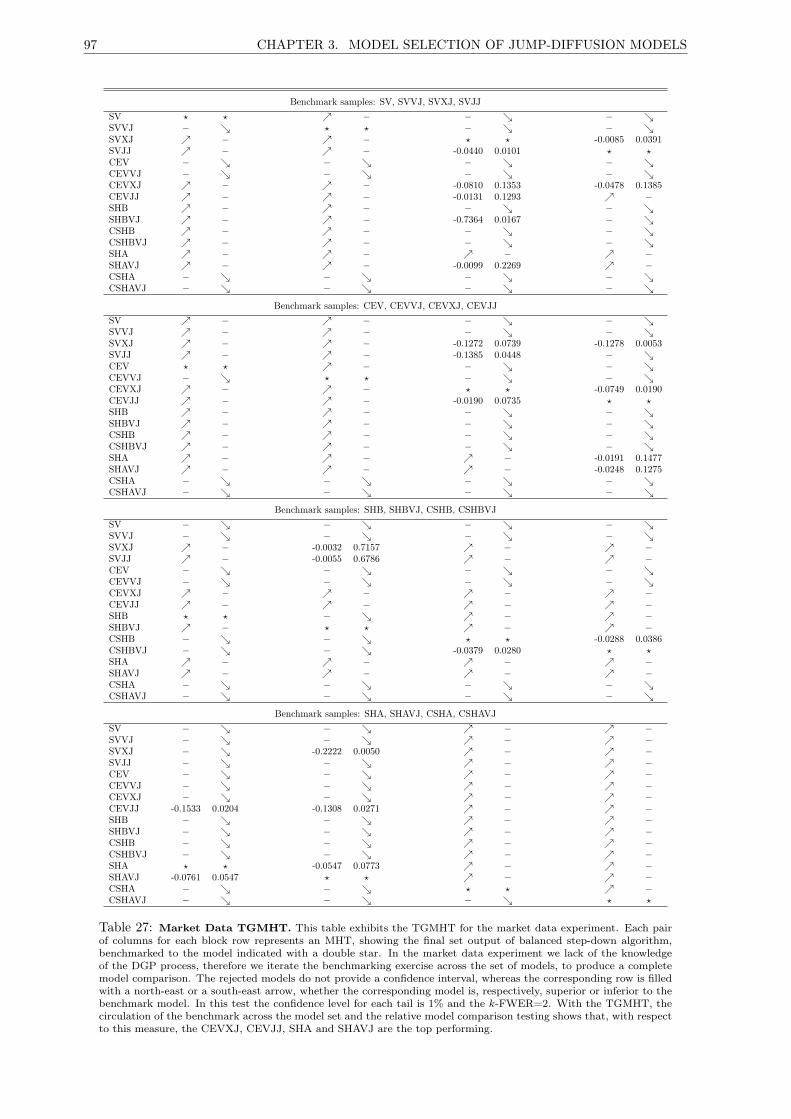
97 CHAPTER 3. MODEL SELECTION OF JUMP-DIFFUSION MODELS
Benchmark samples: SV, SVVJ, SVXJ, SVJJSV ? ? − − − SVVJ − ? ? − − SVXJ − − ? ? -0.0085 0.0391SVJJ − − -0.0440 0.0101 ? ?CEV − − − − CEVVJ − − − − CEVXJ − − -0.0810 0.1353 -0.0478 0.1385CEVJJ − − -0.0131 0.1293 −SHB − − − − SHBVJ − − -0.7364 0.0167 − CSHB − − − − CSHBVJ − − − − SHA − − − −SHAVJ − − -0.0099 0.2269 −CSHA − − − − CSHAVJ − − − −
Benchmark samples: CEV, CEVVJ, CEVXJ, CEVJJSV − − − − SVVJ − − − − SVXJ − − -0.1272 0.0739 -0.1278 0.0053SVJJ − − -0.1385 0.0448 − CEV ? ? − − − CEVVJ − ? ? − − CEVXJ − − ? ? -0.0749 0.0190CEVJJ − − -0.0190 0.0735 ? ?SHB − − − − SHBVJ − − − − CSHB − − − − CSHBVJ − − − − SHA − − − -0.0191 0.1477SHAVJ − − − -0.0248 0.1275CSHA − − − − CSHAVJ − − − −
Benchmark samples: SHB, SHBVJ, CSHB, CSHBVJSV − − − − SVVJ − − − − SVXJ − -0.0032 0.7157 − −SVJJ − -0.0055 0.6786 − −CEV − − − − CEVVJ − − − − CEVXJ − − − −CEVJJ − − − −SHB ? ? − − −SHBVJ − ? ? − −CSHB − − ? ? -0.0288 0.0386CSHBVJ − − -0.0379 0.0280 ? ?SHA − − − −SHAVJ − − − −CSHA − − − − CSHAVJ − − − −
Benchmark samples: SHA, SHAVJ, CSHA, CSHAVJSV − − − −SVVJ − − − −SVXJ − -0.2222 0.0050 − −SVJJ − − − −CEV − − − −CEVVJ − − − −CEVXJ − − − −CEVJJ -0.1533 0.0204 -0.1308 0.0271 − −SHB − − − −SHBVJ − − − −CSHB − − − −CSHBVJ − − − −SHA ? ? -0.0547 0.0773 − −SHAVJ -0.0761 0.0547 ? ? − −CSHA − − ? ? −CSHAVJ − − − ? ?
Table 27: Market Data TGMHT. This table exhibits the TGMHT for the market data experiment. Each pairof columns for each block row represents an MHT, showing the final set output of balanced step-down algorithm,benchmarked to the model indicated with a double star. In the market data experiment we lack of the knowledgeof the DGP process, therefore we iterate the benchmarking exercise across the set of models, to produce a completemodel comparison. The rejected models do not provide a confidence interval, whereas the corresponding row is filledwith a north-east or a south-east arrow, whether the corresponding model is, respectively, superior or inferior to thebenchmark model. In this test the confidence level for each tail is 1% and the k-FWER=2. With the TGMHT, thecirculation of the benchmark across the model set and the relative model comparison testing shows that, with respectto this measure, the CEVXJ, CEVJJ, SHA and SHAVJ are the top performing.
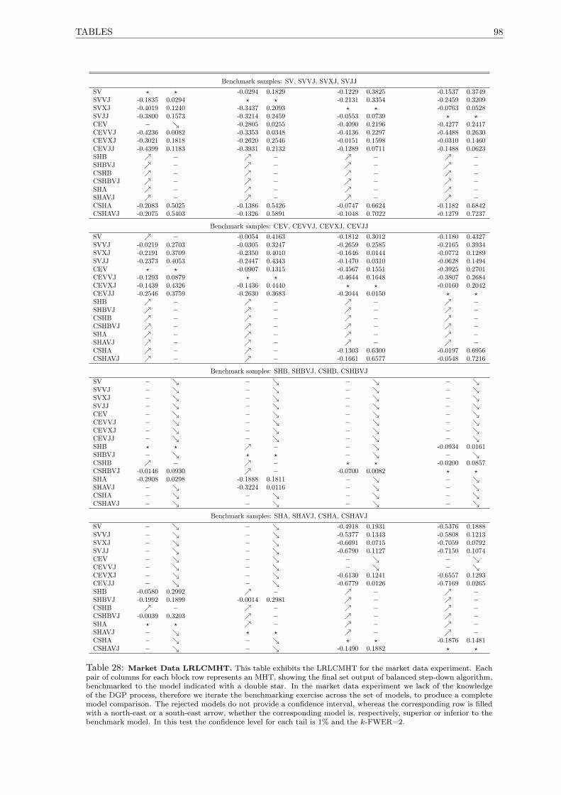
TABLES 98
Benchmark samples: SV, SVVJ, SVXJ, SVJJSV ? ? -0.0294 0.1829 -0.1229 0.3825 -0.1537 0.3749SVVJ -0.1835 0.0294 ? ? -0.2131 0.3354 -0.2459 0.3209SVXJ -0.4019 0.1240 -0.3437 0.2093 ? ? -0.0763 0.0528SVJJ -0.3800 0.1573 -0.3214 0.2459 -0.0553 0.0739 ? ?CEV − -0.2805 0.0255 -0.4090 0.2196 -0.4277 0.2417CEVVJ -0.4236 0.0082 -0.3353 0.0348 -0.4136 0.2297 -0.4488 0.2630CEVXJ -0.3021 0.1818 -0.2620 0.2546 -0.0151 0.1598 -0.0310 0.1460CEVJJ -0.4399 0.1183 -0.3931 0.2132 -0.1289 0.0711 -0.1488 0.0623SHB − − − −SHBVJ − − − −CSHB − − − −CSHBVJ − − − −SHA − − − −SHAVJ − − − −CSHA -0.2083 0.5025 -0.1386 0.5426 -0.0747 0.6624 -0.1182 0.6842CSHAVJ -0.2075 0.5403 -0.1326 0.5891 -0.1048 0.7022 -0.1279 0.7237
Benchmark samples: CEV, CEVVJ, CEVXJ, CEVJJSV − -0.0054 0.4163 -0.1812 0.3012 -0.1180 0.4327SVVJ -0.0219 0.2703 -0.0305 0.3247 -0.2659 0.2585 -0.2165 0.3934SVXJ -0.2191 0.3709 -0.2350 0.4010 -0.1646 0.0144 -0.0772 0.1289SVJJ -0.2373 0.4053 -0.2447 0.4343 -0.1470 0.0310 -0.0628 0.1494CEV ? ? -0.0907 0.1315 -0.4567 0.1551 -0.3925 0.2701CEVVJ -0.1293 0.0879 ? ? -0.4644 0.1648 -0.3807 0.2684CEVXJ -0.1439 0.4326 -0.1436 0.4440 ? ? -0.0160 0.2042CEVJJ -0.2546 0.3759 -0.2630 0.3683 -0.2044 0.0150 ? ?SHB − − − −SHBVJ − − − −CSHB − − − −CSHBVJ − − − −SHA − − − −SHAVJ − − − −CSHA − − -0.1303 0.6300 -0.0197 0.6956CSHAVJ − − -0.1661 0.6577 -0.0548 0.7216
Benchmark samples: SHB, SHBVJ, CSHB, CSHBVJSV − − − − SVVJ − − − − SVXJ − − − − SVJJ − − − − CEV − − − − CEVVJ − − − − CEVXJ − − − − CEVJJ − − − − SHB ? ? − − -0.0934 0.0161SHBVJ − ? ? − − CSHB − − ? ? -0.0200 0.0857CSHBVJ -0.0146 0.0930 − -0.0700 0.0082 ? ?SHA -0.2908 0.0298 -0.1888 0.1811 − − SHAVJ − -0.3224 0.0116 − − CSHA − − − − CSHAVJ − − − −
Benchmark samples: SHA, SHAVJ, CSHA, CSHAVJSV − − -0.4918 0.1931 -0.5376 0.1888SVVJ − − -0.5377 0.1343 -0.5808 0.1213SVXJ − − -0.6691 0.0715 -0.7059 0.0792SVJJ − − -0.6790 0.1127 -0.7150 0.1074CEV − − − − CEVVJ − − − − CEVXJ − − -0.6130 0.1241 -0.6557 0.1293CEVJJ − − -0.6779 0.0126 -0.7169 0.0265SHB -0.0580 0.2992 − − −SHBVJ -0.1992 0.1899 -0.0014 0.2981 − −CSHB − − − −CSHBVJ -0.0039 0.3203 − − −SHA ? ? − − −SHAVJ − ? ? − −CSHA − − ? ? -0.1876 0.1481CSHAVJ − − -0.1490 0.1882 ? ?
Table 28: Market Data LRLCMHT. This table exhibits the LRLCMHT for the market data experiment. Eachpair of columns for each block row represents an MHT, showing the final set output of balanced step-down algorithm,benchmarked to the model indicated with a double star. In the market data experiment we lack of the knowledgeof the DGP process, therefore we iterate the benchmarking exercise across the set of models, to produce a completemodel comparison. The rejected models do not provide a confidence interval, whereas the corresponding row is filledwith a north-east or a south-east arrow, whether the corresponding model is, respectively, superior or inferior to thebenchmark model. In this test the confidence level for each tail is 1% and the k-FWER=2.
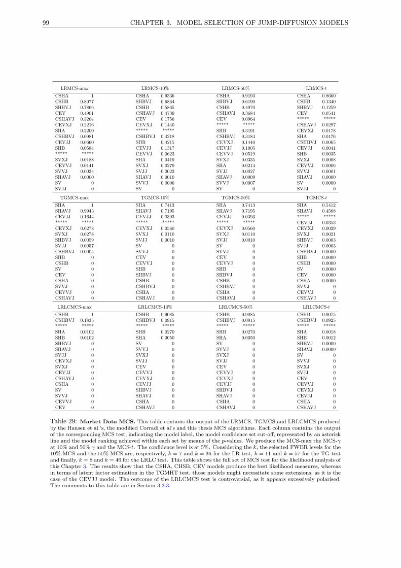
99 CHAPTER 3. MODEL SELECTION OF JUMP-DIFFUSION MODELS
LRMCS-max LRMCS-10% LRMCS-50% LRMCS-tCSHA 1 CSHA 0.9336 CSHA 0.9193 CSHA 0.8660CSHB 0.8077 SHBVJ 0.6864 SHBVJ 0.6190 CSHB 0.1340SHBVJ 0.7866 CSHB 0.5865 CSHB 0.4970 SHBVJ 0.1259CEV 0.4901 CSHAVJ 0.4739 CSHAVJ 0.3684 CEV 0.0541CSHAVJ 0.3264 CEV 0.1756 CEV 0.0964 ***** *****CEVXJ 0.2216 CEVXJ 0.1440 ***** ***** CSHAVJ 0.0297SHA 0.2200 ***** ***** SHB 0.3191 CEVXJ 0.0178CSHBVJ 0.0981 CSHBVJ 0.4218 CSHBVJ 0.3184 SHA 0.0176CEVJJ 0.0660 SHB 0.4215 CEVXJ 0.1440 CSHBVJ 0.0065SHB 0.0584 CEVJJ 0.1317 CEVJJ 0.1005 CEVJJ 0.0041***** ***** CEVVJ 0.0623 CEVVJ 0.0519 SHB 0.0035SVXJ 0.0188 SHA 0.0419 SVXJ 0.0335 SVXJ 0.0008CEVVJ 0.0141 SVXJ 0.0279 SHA 0.0214 CEVVJ 0.0006SVVJ 0.0034 SVJJ 0.0023 SVJJ 0.0027 SVVJ 0.0001SHAVJ 0.0000 SHAVJ 0.0010 SHAVJ 0.0009 SHAVJ 0.0000SV 0 SVVJ 0.0006 SVVJ 0.0007 SV 0.0000SVJJ 0 SV 0 SV 0 SVJJ 0
TGMCS-max TGMCS-10% TGMCS-50% TGMCS-tSHA 1 SHA 0.7413 SHA 0.7413 SHA 0.5412SHAVJ 0.9943 SHAVJ 0.7195 SHAVJ 0.7195 SHAVJ 0.4588CEVJJ 0.1644 CEVJJ 0.0393 CEVJJ 0.0393 ***** ********** ***** ***** ***** ***** ***** CEVJJ 0.0353CEVXJ 0.0278 CEVXJ 0.0560 CEVXJ 0.0560 CEVXJ 0.0029SVXJ 0.0278 SVXJ 0.0110 SVXJ 0.0110 SVXJ 0.0021SHBVJ 0.0059 SVJJ 0.0010 SVJJ 0.0010 SHBVJ 0.0003SVJJ 0.0057 SV 0 SV 0 SVJJ 0.0003CSHBVJ 0.0004 SVVJ 0 SVVJ 0 CSHBVJ 0.0000SHB 0 CEV 0 CEV 0 SHB 0.0000CSHB 0 CEVVJ 0 CEVVJ 0 CSHB 0.0000SV 0 SHB 0 SHB 0 SV 0.0000CEV 0 SHBVJ 0 SHBVJ 0 CEV 0.0000CSHA 0 CSHB 0 CSHB 0 CSHA 0.0000SVVJ 0 CSHBVJ 0 CSHBVJ 0 SVVJ 0CEVVJ 0 CSHA 0 CSHA 0 CEVVJ 0CSHAVJ 0 CSHAVJ 0 CSHAVJ 0 CSHAVJ 0
LRLCMCS-max LRLCMCS-10% LRLCMCS-50% LRLCMCS-tCSHB 1 CSHB 0.9085 CSHB 0.9085 CSHB 0.9075CSHBVJ 0.1835 CSHBVJ 0.0915 CSHBVJ 0.0915 CSHBVJ 0.0925***** ***** ***** ***** ***** ***** ***** *****SHA 0.0102 SHB 0.0270 SHB 0.0270 SHA 0.0018SHB 0.0102 SHA 0.0050 SHA 0.0050 SHB 0.0012SHBVJ 0 SV 0 SV 0 SHBVJ 0.0000SHAVJ 0 SVVJ 0 SVVJ 0 SHAVJ 0.0000SVJJ 0 SVXJ 0 SVXJ 0 SV 0CEVXJ 0 SVJJ 0 SVJJ 0 SVVJ 0SVXJ 0 CEV 0 CEV 0 SVXJ 0CEVJJ 0 CEVVJ 0 CEVVJ 0 SVJJ 0CSHAVJ 0 CEVXJ 0 CEVXJ 0 CEV 0CSHA 0 CEVJJ 0 CEVJJ 0 CEVVJ 0SV 0 SHBVJ 0 SHBVJ 0 CEVXJ 0SVVJ 0 SHAVJ 0 SHAVJ 0 CEVJJ 0CEVVJ 0 CSHA 0 CSHA 0 CSHA 0CEV 0 CSHAVJ 0 CSHAVJ 0 CSHAVJ 0
Table 29: Market Data MCS. This table contains the output of the LRMCS, TGMCS and LRLCMCS producedby the Hansen et al.’s, the modified Corradi et al’s and this thesis MCS algorithms. Each column contains the outputof the corresponding MCS test, indicating the model label, the model confidence set cut-off, represented by an asteriskline and the model ranking achieved within each set by means of the p-values. We produce the MCS-max the MCS-γat 10% and 50% γ and the MCS-t. The confidence level is at 5%. Considering the k, the selected FWER levels for the10%-MCS and the 50%-MCS are, respectively, k = 7 and k = 36 for the LR test, k = 11 and k = 57 for the TG testand finally, k = 8 and k = 46 for the LRLC test. This table shows the full set of MCS test for the likelihood analysis ofthis Chapter 3. The results show that the CSHA, CHSB, CEV models produce the best likelihood measures, whereasin terms of latent factor estimation in the TGMHT test, those models might necessitate some extensions, as it is thecase of the CEVJJ model. The outcome of the LRLCMCS test is controversial, as it appears excessively polarised.The comments to this table are in Section 3.3.3.
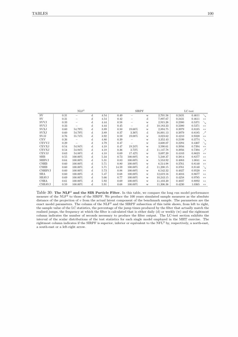
TABLES 100
NLF2 SIRPF LC-testSV 0.31 − d 4.54 0.49 − w 2,701.56 0.2431 0.4611 SV 0.31 − d 4.54 0.42 − d 7,897.67 0.2431 0.4611 ↔SVVJ 0.33 − d 4.44 0.58 − w 2,915.26 0.2380 0.5371 SVVJ 0.33 − d 4.44 0.45 − d 10,183.33 0.2380 0.5371 ↔SVXJ 0.60 54.79% d 3.89 0.50 19.66% w 2,894.75 0.3979 0.8185 ↔SVXJ 0.60 54.79% d 3.89 0.37 3.36% d 16,001.13 0.3979 0.8185 SVJJ 0.76 55.74% d 3.92 0.59 19.08% w 3,023.62 0.4210 0.9320 ↔CEV 0.26 − d 4.80 0.39 − w 3,352.43 0.2199 0.3774 CEVVJ 0.29 − d 4.79 0.47 − w 3,608.07 0.2294 0.4307 CEVXJ 0.54 54.94% d 4.18 0.47 19.24% w 3,590.61 0.3956 0.7394 ↔CEVXJ 0.54 54.94% d 4.18 0.36 3.73% d 11,147.78 0.3956 0.7394 CEVJJ 0.63 54.88% d 4.18 0.69 17.42% w 3,697.20 0.4183 0.8623 ↔SHB 0.55 100.00% d 5.34 0.73 100.00% w 5,248.37 0.3814 0.8277 ↔SHBVJ 0.64 100.00% d 5.31 0.83 100.00% w 5,553.92 0.4083 1.0041 ↔CSHB 0.60 100.00% d 5.71 0.80 100.00% w 6,514.98 0.3761 0.8140 ↔CSHB 0.60 100.00% d 5.71 14.59 100.00% d 11,200.15 0.3761 0.8140 CSHBVJ 0.60 100.00% d 5.73 0.88 100.00% w 6,542.32 0.4027 0.9520 ↔SHA 0.60 100.00% d 5.47 0.68 100.00% w 12,619.16 0.4016 0.8677 ↔SHAVJ 0.69 100.00% d 5.66 0.77 100.00% w 10,243.15 0.4258 0.9785 ↔CSHA 0.61 100.00% d 5.92 0.69 100.00% w 11,103.20 0.4037 0.8892 ↔CSHAVJ 0.59 100.00% d 5.91 0.68 100.00% w 11,306.36 0.4230 1.0365 ↔
Table 30: The NLF2 and the SIR Particle Filter. In this table, we compare the long run model performancemeasure of the NLF2 to those of the SIRPF. We produce the 100 years simulated sample measures as the absolutedistance of the projection of v from the actual latent component of the benchmark sample. The parameters are theexact model parameters. The column of the NLF2 and the SIRPF subsection of this table shows, from left to right,the sample value of the LC statistics, the percentage of the jump times produced by the filter that actually match therealised jumps, the frequency at which the filter is calculated that is either daily (d) or weekly (w) and the rightmostcolumn indicates the number of seconds necessary to produce the filter output. The LC-test section exhibits theinterval of the scalar distributions of the test statistics for each single model employed in the MHT exercise. Therightmost column indicates if the SIRPF is superior, inferior or equivalent to the NFL2 by, respectively, a north-east,a south-east or a left-right arrow.

101 CHAPTER 3. MODEL SELECTION OF JUMP-DIFFUSION MODELS
.
Figure 1: The Likelihood Function Algorithm.
The figure shows 4 sections that are labelled from a to d in matrix order. Section (a) shows the marginaliseddensity of the simulation SV model. Section (b) depicts the bivariate densities on the grid of initial condition forv, ranging from (almost) 0 to seven times the projected variance over the weekly horizon. The initial condition forx is centred at 0 for each grid-point of v. The (c) quadrant shows the conditional marginals that are weighted bythe stationary distribution of the initial conditions for v, as shown in the section (d).
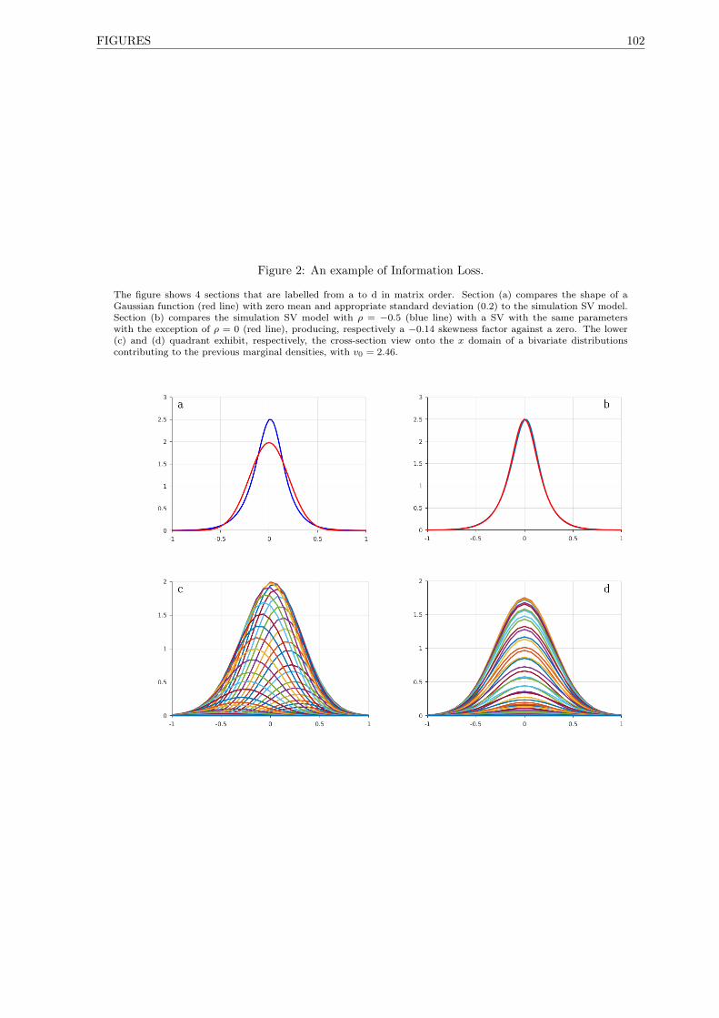
FIGURES 102
Figure 2: An example of Information Loss.
The figure shows 4 sections that are labelled from a to d in matrix order. Section (a) compares the shape of aGaussian function (red line) with zero mean and appropriate standard deviation (0.2) to the simulation SV model.Section (b) compares the simulation SV model with ρ = −0.5 (blue line) with a SV with the same parameterswith the exception of ρ = 0 (red line), producing, respectively a −0.14 skewness factor against a zero. The lower(c) and (d) quadrant exhibit, respectively, the cross-section view onto the x domain of a bivariate distributionscontributing to the previous marginal densities, with v0 = 2.46.

103 CHAPTER 3. MODEL SELECTION OF JUMP-DIFFUSION MODELS
Figure 3: The Distributional Shape of the Model Set.
The figure shows 4 sections that are labelled from a to d in matrix order. In this figure, the SV model (bluecurve) marginal distribution is compared with several other members of the model set, computed at the simulationparameters. Frame (a) shows some kurtosis generated by ancillary model components, as in the case of the SVVJ(red line) and the CEVVJ (light blue line) model. In the SVXJ (red line) model of frame (b) and in the SHB (redline) and the CSHBVJ (dashed light blue line) of frame (c), asymmetry can be generated by jumps. In the (d)quadrant, the marginal densities of two stochastic hazard models with skewed Normal jumps are plotted againstthe SV profile, that is the SHA (red curve) and the CSHAVJ.
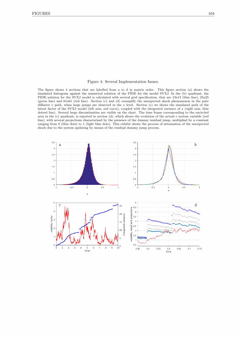
FIGURES 104
Figure 4: Several Implementation Issues.
The figure shows 4 sections that are labelled from a to d in matrix order. This figure section (a) shows thesimulated histogram against the numerical solution of the PIDE for the model SVXJ. In the (b) quadrant, thePIDE solution for the SVXJ model is calculated with several grid specification, that are 13x13 (blue line), 25x25(green line) and 61x61 (red line). Section (c) and (d) exemplify the unexpected shock phenomenon in the purediffusive v path, when large jumps are observed in the x level. Section (c) we shows the simulated path of thelatent factor of the SVXJ model (left axis, red curve), coupled with the integrated variance of x (right axis, bluedotted line). Several large discontinuities are visible on the chart. The time frame corresponding to the encircledarea in the (c) quadrant, is reported in section (d), which shows the evolution of the actual v system variable (redline), with several projections characterised by the presence of the dummy residual jump, multiplied by a constantranging from 0 (blue dots) to 1 (light blue dots). This exhibit shows the process of attenuation of the unexpectedshock due to the system updating by means of the residual dummy jump process.

105 CHAPTER 3. MODEL SELECTION OF JUMP-DIFFUSION MODELS
Figure 5: Market Data Applications.
The figure shows 4 sections that are labelled from a to d in matrix order. Section (a) shows the cumulative log return(times 100) path employed for market data testing. The (b) quadrant exhibits the histogram of daily returns withthe superimposed estimated CSHB marginal likelihood. Section (c) shows a segment of the TGARCH estimatedvolatility (red line) and the scaled and translated output of the NLF2 (blue line) for the CEVJJ process, as appliedto market data. The lower-right picture (d) shows a portion of the actual v path (red line) for the SV simulatedprocess, with the SIRPF output path (green line) and the NLF2 projected latent component (blue line).


107 CHAPTER 4. MODEL SELECTION OF DERIVATIVE PRICING JD MODELS
Model Selection of
Derivative Pricing JD Models
In this chapter, we explore the model selection problem in the context of option pricing models. The
general focus is on several formulations of stochastic volatility models that in their broadest specification
include jump components. As noticed in Christoffersen et al. (2010), the literature on stochastic volatility
models can be grouped into three branches. In Chapter 3, we have tackled the analysis of the daily return
distribution of financial returns from a time-series perspective, including alternative models within the
affine set, a study which falls within the first body of research. The second set of studies concerns the
analysis of realised volatility or volatility proxies to forecast future volatility, examples of which are Bakshi
et al. (2006), Aït-Sahalia and Kimmel (2007). The latter overlaps to some extent with the general option
pricing literature, which forms the last body of econometric studies of stochastic volatility models and
to which this chapter contributes. Seminal studies in this subject are represented by the works of Bates
(1996) and Bakshi et al. (1997), which both set standards in the model performance analysis by exam-
ining measures of in-sample and out-of-sample mispricing, option implied stochastic process features as
compared to the underlying return and implicit volatility behaviour, single-instrument and delta-neutral

108
hedge analysis. The literature mainly works within the affine framework, as a consequence of the stylised
approach originated in Heston (1993), Duffie and Kan (1996), Duffie et al. (2000) and the computational
efficiency that integral transform methods generally offer in terms of option pricing and hedge measure
calculation. Examples of studies that compare affine models versus alternative model specifications using
option data, but not strictly in an option mispricing context, are those in Benzoni (2002), Jones (2003)
and Aït-Sahalia and Kimmel (2007). The first article exploits log-normal volatility as an alternative,
whereas the latter two both employ a volatility CEV model, which is complemented with a GARCH
stochastic volatility in the most recent one. The non affine model in Benzoni (2002) appears unable to
outperform the Heston model, whereas the evidence in Jones (2003) and Aït-Sahalia and Kimmel (2007)
points to a misspecification of the affine model. A further extension in the analysis of stochastic volatility
models with contrasting alternatives to the affine specification is the cited work of Christoffersen et al.
(2010), which employs a wide database including realised volatility, S&P500 returns and a panel of op-
tion data. The model set is diverse and includes several alternative volatility specifications that perform
better than the affine model under several measures. The cited works, however, employ mainly diffusion
models, although evidence suggesting the need for discontinuous extensions is inferred from short-term
OTM pricing model behaviour. Empirical works using JD models can be found, for instance, in Bates
(1996, 2000), Pan (2002), Eraker et al. (2003) and Eraker (2004), which all apply the affine framework
with combinations of constant or stochastic intensity and independent or correlated jumps in volatility
and returns. The general result is that jumps improve the option pricing performance with a preference
for joint jumps in return and volatility. The performance of the stochastic intensity model does not seem
to improve the overall model yield. Those articles model the volatility jump size with an exponential
distribution and the price jump size at most with an offset log-normal distribution.
In our analysis, we gather evidence that the popular single factor affine specification common in the liter-
ature are strongly rejected. Moreover, model augmentation such as jumps in volatility, stochastic hazard,
and the parametrisation of the elasticity of the diffusion factor, appear to be excessive model complica-
tions. A simple model, such as the log-normal correlated volatility model, performs very well in the OTM
option sample we consider, whereas the inclusion of a compensated single directional exponential jump
in return produces one of the top performance for the ALL option sample. We also sketch a qualitative
comparison among the established Hansen et al. (2011) MCS test and our original γ-MCS test, developed
within the MHT framework of Romano and Wolf (2010), whereby we provide evidence that the latter
test can offer a wider flexibility allowed by the k-FWER controlling mechanism. This chapter therefore
provides several contributions. First, we construct a novel model selection test that, for the first time in
literature, is using a vast array of option pricing models, containing 280 model specifications in today,
the majority of which are obtained by uniquely combining jumps and volatility specifications in a way
never explored before in the literature. Second, we exploit for the first time the power of MHT and MCS
techniques, specifically the max -MCS and our novel MHT consistent γ-MCS, in an option pricing model
comparison exercise. Third, by selecting the subset of best performing equivalent models, we are also
able to infer conclusion about the model similarity hypothesis and provide empirical evidence of strong
aliasing amongst many option pricing models ranging from high to a lower level of complexity, whereby
complexity may be ascribed to the size of the parameter vector.

109 CHAPTER 4. MODEL SELECTION OF DERIVATIVE PRICING JD MODELS
We exploit the finite difference method (FDM) combined with numerical integration to construct the
solution of the pricing equation for a large collection of JD models. The references for the finite difference
method are represented, for instance, by Tavella and Randall (2000), Duffy (2006). The model set can be
mainly divided into two families of stochastic volatility models, characterised by affine volatility (Heston,
1993) or by volatility generated with the exponential of a Gaussian mean-reverting process (Scott, 1987).
The latent factor can include an exponential jump component. The models are augmented with elasticity
of variance parameters and with a wide range of jump specifications in the price process, endowed with
stochastic hazard in their more complex specifications. The model selection exercise conducted in this
chapter applies the main MCS tests constructed in Chapter 1, with the objective of the mean squared
error (MSE) measure of mispricing as the model performance loss function.
The work is organised as follows. In Section 4.1 we introduce the model set and describe the model dy-
namics features. Section 4.2 introduces the testing set-up, whereas Section 4.3 details the implementation
of the test and describes the results. Section 4.4 offers concluding remarks.
4.1 The Derivative Pricing Model Set
With the empirical exercise in this study, we employ a very large model set of equity derivative pricing
models to test for the MCS. The model collection contains two major families of stochastic volatility mod-
els, whereby the volatility factor is either modelled as an affine process as in the Heston (1993) model, or
it is generated by a mean reverting Geometric Brownian motion, as in the Scott (1987) model. We extend
the model set represented by affine jump-diffusion specifications as evidence supporting faster than affine
acceleration of the volatility factor are common in the econometrics of financial markets literature, see for
instance Jones (2003), Christoffersen et al. (2010). The stochastic volatility factor defining the diffusion
function is either square rooted or powered by a free parameter, allowing for extended CEV specifications
in the affine case or for linear elasticity1 of variance (LEV) in the geometric variance case. The model
diffusive dynamics is also combined with Poisson jumps under several specifications. The jumps can
affect the model price and volatility processes, which can jump independently or simultaneously. The
price jump process can also allow for stochastic intensity, which under this configuration is coupled with
stochastic diffusion. We do not include here high frequency jump models, as we have already established
in Chapter 3 that they are equivalent to more orthodox models, which are the focus of this analysis. In
the execution of the exercise, we are also interested in testing the contribution to the model performance
of the diffusion correlation factor (ρ), as we test models with or without the leverage effect. Combining
the inclusion or exclusion of the cited model components with the several specifications of the volatility
and the jump factors, we obtain a collective of 280 models. The full model set is split into two groups
characterised by the alternative specifications of the latent factor. In general, the model structure is
1 We include the LEV parameter in the geometric mean-reverting specification of the stochastic diffusion factor, in orderto parallel the flexibility of the elasticity of diffusion that is provided by the CEV model. However, as it is shown inAppendix A.4, in the log-normal model this parameter simply acts as an amplifier of the variability of the v factor entailingwider excursions of the diffusion process. This feature can as well be obtained by changing the θ value, although with adifferent sensitivity of the model performance measure to the parameter variations.
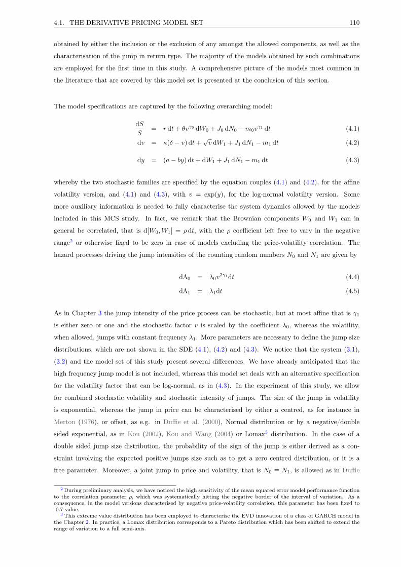
4.1. THE DERIVATIVE PRICING MODEL SET 110
obtained by either the inclusion or the exclusion of any amongst the allowed components, as well as the
characterisation of the jump in return type. The majority of the models obtained by such combinations
are employed for the first time in this study. A comprehensive picture of the models most common in
the literature that are covered by this model set is presented at the conclusion of this section.
The model specifications are captured by the following overarching model:
dS
S= r dt+ θvγ0 dW0 + J0 dN0 −m0v
γ1 dt (4.1)
dv = κ(δ − v) dt+√v dW1 + J1 dN1 −m1 dt (4.2)
dy = (a− by) dt+ dW1 + J1 dN1 −m1 dt (4.3)
whereby the two stochastic families are specified by the equation couples (4.1) and (4.2), for the affine
volatility version, and (4.1) and (4.3), with v = exp(y), for the log-normal volatility version. Some
more auxiliary information is needed to fully characterise the system dynamics allowed by the models
included in this MCS study. In fact, we remark that the Brownian components W0 and W1 can in
general be correlated, that is d[W0,W1] = ρdt, with the ρ coefficient left free to vary in the negative
range2 or otherwise fixed to be zero in case of models excluding the price-volatility correlation. The
hazard processes driving the jump intensities of the counting random numbers N0 and N1 are given by
dΛ0 = λ0v2γ1dt (4.4)
dΛ1 = λ1dt (4.5)
As in Chapter 3 the jump intensity of the price process can be stochastic, but at most affine that is γ1
is either zero or one and the stochastic factor v is scaled by the coefficient λ0, whereas the volatility,
when allowed, jumps with constant frequency λ1. More parameters are necessary to define the jump size
distributions, which are not shown in the SDE (4.1), (4.2) and (4.3). We notice that the system (3.1),
(3.2) and the model set of this study present several differences. We have already anticipated that the
high frequency jump model is not included, whereas this model set deals with an alternative specification
for the volatility factor that can be log-normal, as in (4.3). In the experiment of this study, we allow
for combined stochastic volatility and stochastic intensity of jumps. The size of the jump in volatility
is exponential, whereas the jump in price can be characterised by either a centred, as for instance in
Merton (1976), or offset, as e.g. in Duffie et al. (2000), Normal distribution or by a negative/double
sided exponential, as in Kou (2002), Kou and Wang (2004) or Lomax3 distribution. In the case of a
double sided jump size distribution, the probability of the sign of the jump is either derived as a con-
straint involving the expected positive jumps size such as to get a zero centred distribution, or it is a
free parameter. Moreover, a joint jump in price and volatility, that is N0 ≡ N1, is allowed as in Duffie
2 During preliminary analysis, we have noticed the high sensitivity of the mean squared error model performance functionto the correlation parameter ρ, which was systematically hitting the negative border of the interval of variation. As aconsequence, in the model versions characterised by negative price-volatility correlation, this parameter has been fixed to-0.7 value.
3 This extreme value distribution has been employed to characterise the EVD innovation of a class of GARCH model inthe Chapter 2. In practice, a Lomax distribution corresponds to a Pareto distribution which has been shifted to extend therange of variation to a full semi-axis.
111 CHAPTER 4. MODEL SELECTION OF DERIVATIVE PRICING JD MODELS
et al. (2000). In this case the intensity is allowed to be constant only. Further difference lies in the
observable S, which would be the corresponding geometric process of the cumulative return x in (3.1)
of Chapter 3 that is taken at the risk-neutral measure, entailing a drift at the constant interest rate r.
In this chapter, the main reason for designing the system with respect to the S variable, is found in the
nature of the problem, which includes the observable index level and the option prices as functions of
the former, whereas in the previous set of experiments the price is otherwise observed as a log-return
curve. Listing other differences when compared to the system of the previous chapter, we observe that
the Poisson jump of S is compensated locally by including the possibly stochastic hazard factor. Another
difference which is experimented here is the standardisation of the volatility acceleration, which implies
an adjustment factor4 in the unitary mean of (3.1). In terms of parameter definitions, we notice that the
coefficient r is the constant interest rate, corresponding to the instantaneous equivalent rate of the three
months LIBOR rate. The parameter r is assumed to be constant, although during the optimisation the
interest rate is observed daily. As noticed in Scott (1997), stochastic interest rates have a limited impact
on short dated options. Further parameters are represented by the diffusion process scaling factor θ, as
we rescale the latent component to have unitary diffusion parameter. The diffusion component in (4.1)
is powered to the γ0 coefficient, which controls CEV and LEV effects, respectively for the affine and the
log-normal volatility model. As mentioned earlier, the jump process is compensated in order to obtain the
martingale∑N0(t)i=1 Sτi
(J0,i − m0
λ0Λ0(t)
)and therefore m0 represents simply the intensity scaling factor
λ0 times the expectation of J0 ≡ z in the case of the Lomax distribution and J0 ≡ ez with all other
distribution hypotheses. We choose the former configuration for the extreme value distribution (EVD),
as it lacks of finite exponential moments. In Eq. (4.2) we describe the latent factor specification of the
affine/CEV family, whereby the parameter κ represents the speed of mean reversion and δ the mean level
of v. Under this specification, we scale the conventional stochastic volatility factor in order to obtain an
unitary coefficient in the diffusion component. This choice is motivated by the intention to simplify the
estimation of the latent component by moving some parameters either onto the observable or at least
onto its first order component5. In the case of the log-normal latent component of Eq. (4.3), the speed
of mean reversion is represented by the coefficient b, whereas the mean level is represented by the ratio
a/b. Both the latent components might include a constant intensity exponential jump J1, compensated
by the opposite sign of the Poisson process drift m1.
The affine specification in Eq. (4.1) and (4.2) embeds the Heston (1993) model. Under independent or
dependent Normal jumps in price and exponential jumps in volatility it contains the models in Duffie et al.
(2000) and Eraker et al. (2003), while under stochastic hazard the (single factor) model of Bates (2000)
augmented with jumps in volatility is also captured. The jumps can be negative sided or double sided, with
appropriate compensation factor or, in the case of double jumps, the compensation is embedded within
constrained probability of positive/negative jumps. The double exponential jump of Kou (2002) and Kou
and Wang (2004) is augmented with stochastic volatility and intensity. A novel jump specification is
represented by the EVD jump model. Moreover, the stochastic volatility family of this study is expanded
4 To standardise the stochastic volatility diffusion from the Eq. (3.1), we simply set u = v/σ2 and rewrite the system,adjusting the drift and the volatility factor of x. In Eq. (4.1) and (4.2), we have kept the same variable and parameterdenomination as in Chapter 3, whereby the affine model of this study can be easily reverted to the previous type.
5 See Appendix A.4 for further details concerning the transformations of the conventional models adopted in this study.

4.2. MODEL COMPARISON TESTING 112
with a mean-reverting log-normal stochastic volatility model as in Scott (1987), also (partially) introduced
during the same year by Wiggins (1987) and Hull and White (1987), whereby the diffusion is augmented
with the collection of jumps just outlined. The CEV specifications can also be allowed, which in the case
of affine volatility can be seen as an extension of the models in Beckers (1980), Macbeth and Merville
(1980) but also, under a transformation, can be related to the CEV stochastic volatility model class used
in Jones (2003) and Aït-Sahalia and Kimmel (2007). As to our knowledge, the LEV specification under
the log-normal volatility model is a novel application. Certain model components combination are also
explored for the first time in the literature. Specifically, these models comprise: stochastic volatility
combined with exponential and Lomax jumps; the log-normal volatility model combined with stochastic
intensity and with the further jump specification generating joint jumps; models that allow jumps in
volatility only. In Appendix A.4 we specify which transformation should be performed to connect the
models of this study to more conventional models used in the literature. In Section 4.3.1, we will be
presenting a labelling scheme to identify the model configurations in the context of the testing results.
4.2 Model Comparison Testing
In the experimental section of this chapter, we apply the max -MCS test introduced in Section 1.3.1 and
construct the MHT (1.3) combined with the MCS algorithm as in Section 1.3.3, to produce an option
model mispricing exercise with the reference MCS test and the novel γ-MCS presented in this thesis. The
goal is the selection of the best set of models producing the lowest MSE when applied to a large sample
of option market data. Option pricing for affine models is usually pursued with the Fourier inversion
technique introduced in Heston (1993) and refined in Carr and Madan (1999). A multidimensional general
Fourier inversion technique is presented in Shephard (1991a,b). In the context of the Scott model, a quasi-
analytic solution exploiting the Laplace transform is found in Perelló et al. (2008). Another technique
traditionally used for pricing alternative models consists of the recombining tree method, introduced in
Finance by Cox and Ross (1976). Simulation is also widely used in the financial community for derivative
pricing, see for instance Platen and Bruti-Liberati (2010) to construct a multidimensional JD simulation
with pre-specified order of convergence. An alternative technique is represented by the quasi-analytic
approximation of the price density constructed in Aït-Sahalia (1999, 2008). In this study, we use PIDE
solution techniques, see for example Tavella and Randall (2000), Duffy (2006). To generate the bootstrap
samples and the summary statistics feeding the MCS algorithms, we exploit the FDM6 to construct a
numerical solution of the backward equation defining the European call/put option price
EQ [(ST −K)± |Ft]
e−r(T−t) (4.6)
where the interest rate is assumed non-stochastic. We employ the martingale approach to achieve the
derivative price, as we have constructed the SDE describing the underlying’s dynamics in (4.1) as such
that discounting the price by a non-stochastic or non-correlated factor, a martingale process is obtained.
The solution of the expectation in (4.6) is generated by means of the Fokker-Planck equation approach,
as mentioned above. It is acknowledged that in the case of a complete market, the martingale approach
6 For further details regarding the implemented procedure, compare Appendix A.2.

113 CHAPTER 4. MODEL SELECTION OF DERIVATIVE PRICING JD MODELS
and the risk-neutral technique, achieved by the construction of a risk-less replicating portfolio, are both
equivalent, see for instance Musiela and Rutkowski (1997). However, when the market is not complete,
that is some risk factors are not traded, as is the case for the asset volatility, the pricing equation
obtained via the hedging argument is not unique, see for instance Scott (1987). Thus, usually the market
equilibrium argument is invoked and a “market risk premium” is introduced. For practical purposes,
the introduction of risk premia usually has the effect of altering the parameters of some risk factors,
without changing the overall structure of the main SDE. The analysis of the effect of market risk premia
on the main equation is beyond the scope of this thesis. For an interesting analysis concerning the
estimation of risk-premia in JD models, see for instance Pan (2002). In order to simplify the complexity
of the computations, the strike price K is taken out of the pay-off function and the underlying variable
redefined as sT = ST /K, which evolves according to the reference dynamics, that is Eqs. (4.1) and
(4.2)/(4.3), but with initial condition st. In practice, each option price O±j , where the plus and minus
signs refer, respectively, to the call and put option, corresponds to the present value of the strike times
a stochastic factor depending on stj and the model parameters, whereas the relative strike is always
unitary. That is,
O±j (Tj , stj ; Θ, vtj ) = EQ [(sTj − 1)±∣∣Ftj ]Kje
−r(Tj−tj) (4.7)
and we conduct the analysis in terms of the relative option prices ω±j = O±j /Kj . We adopt this strategy
in contrast to the usage of dollar prices as in Bakshi et al. (1997) that induces dependence on the index
level and therefore the time of the price record. This procedure is also alternative to the option price
standardisation of Bates (1996, 2000), which operates with option-to-underlying price ratios. As we solve
the option pricing problem with a PIDE solution method, it is natural to standardise the underlying by
the strike and not viceversa, whereby this strategy only modifies the initial condition of the reference
underlying at the same time anchoring any instrument in the sample to a unitary strike. As a consequence,
the complexity of the problem is simplified because in this way, we are centring the solution domain over
a given range initiated by a unique terminal condition. The reverse strategy instead, that is dividing
the option price by the underlying level, virtually changes the nature of the problem, as we are now in
the presence of a stochastic strike option over a constant reference underlying. Moreover, although not
interested into the hedging problem here, we notice that the latter strategy complicates any perturbation
analysis as the computation of the sensitivity effect are more involved7. In the following, unless otherwise
explicitly stated, when we write of option prices we will be referring to relative option prices.
4.2.1 Mispricing MSE
The model performance measure we use in this study is the mispricing, that is the average squared
difference between model prices and actual prices, or its square root (RMSE). The MSE is essentially a
measure of the goodness of fit of the model across the set of observed data; the lower the mispricing,
7 In fact, from a numerical perspective, because when standardising by the strike the initial condition of the PIDE isunique for any option data set, the computation of the numerical derivative will only involve as many solution as the chosenfinite difference would require, whereas standardising by the current level of the strike will have the effect of multiplyingthe latter number by the number of strikes in the sample. Another complication for the computation of the ∆ is that, inthe former case, variations of the current price level will only impact the standardised underlying linearly and therefore thevariations will simply be proportional to the strike, whereas in the latter case variations of the underlying will impact theinitial condition non linearly entailing a distortion of the ∆ range or more articulated calculations to reconstruct the nonstandardised effect.
4.2. MODEL COMPARISON TESTING 114
the better the model explains the realised market quotes. It is important to notice that the use of
the MSE requires the standardisation of the option prices, in order to get rid of the dependency on
the money value of the strike. Moreover, the choice of standardising by the strike, rather than the
underlying price value as it is customary in other articles, as for instance Bates (2000), gives to the option
relative value the immediate significance of a dimensionless measure of “moneyness”, that is a relative
number indicating how deep in the money the option is, whereas standardising by the current level of the
underlying turns this quantity in the opposite direction, whereby lower numbers would indicate higher
moneyness and viceversa, lacking of an intuitive significance. Dropping for convenience the reference to
the moneyness and the tenor of the option and highlighting the dependency on the parameter vector Θ
and the market volatility information, the loss function for the generic model Pi is described as following,
using information across the full time span of the sample:
Li := 1N
∑j
(ωj(Θi, v
itj )− ϕj
)2
(4.8)
whereby ϕj is the j-th market implied option price, with tj = t, ∀t, j, and vit the model Pi volatility at
time8 t. In Eq. (4.8) more information is necessary to determine the model price of the ϕj , which we
do not make explicit; namely, the option type, the underlying level-to-strike ratio providing the initial
condition for the pricing engine, the tenor of the option and the current interest rate level. With respect
to the latter model components, we notice that the parameter vector Θ∗i and the estimated volatility
sample pathvikKk=1
for the model Pi are the output of the following program
minΘi,vikKk=1
Li (4.9)
The estimation of the parameter vector Θ is performed as follows. The target MSE function is constructed
such that, for a given Θ, the loss function L, at each observation date k = 1, . . . ,K, is evaluated over a
grid spanning the domain of definition of the latent variable v and thus the sequence vkKk=1 is selected
such as to render the least loss. It is implied that the grid is determined by the restriction of the current
parameters to those defining the v process, such that the domain of definition spreads between zero
and seven times the long run model volatility, whereas the number of points is fixed and proportionally
distributed amid the boundaries. In practice, at each evaluation given the parameters Θ, the loss function
returns the minimum value amongst all the possible determinations over the vk sequence, determined over
the current grid. The parameter vector Θ is hence optimised by sequential quadratic programming. As a
consequence, the optimisation problem (4.9) is divided into two sub-problems: the main one consists of
numerically minimising Li with respect to Θi and the secondary one provides the minimum Li |Θi with
respect to the sequence of model implied volatility, refining the target function for the main problem. We
make a point in this latter analysis of applying a given set of parameters across the time dimension of
the price sample, thereby focusing on the stochastic volatility models ability to reproduce market prices
by the means of the latent factor only. This bestows upon the solution strategy the nature of a highly
8 In order to summarise the procedure, we have appended a subscript j to each option price in the data panel, entailingthat an ordered record of market option prices and their corresponding model generated values is available. Because thevolatility factor is an essential input of the model price, its estimate will enter each model determination, whereby the dailyvt is cross-referenced to the determination of the j-th options that will be given at market time tj , that is the referencevolatility at time t is attributed to each j-th option at day t.

115 CHAPTER 4. MODEL SELECTION OF DERIVATIVE PRICING JD MODELS
parametrised problem, as in Bates (2000). We choose to solve the problem (4.9) over a coarse grid of the
volatility within a plausible range of variation, given the current set of parameters. Although we do not
employ any filtering technique, the projected path can be considered as a suboptimal solution achieved
with reasonable speed of computation.
4.3 Experimental Section
4.3.1 Preliminary Considerations
In this section, we produce several MCS tests to select the best option pricing models from a collection
of Heston (1993) and Scott (1987) stochastic volatility models feeding a diffusion function that can be,
respectively, linear or exponential and is extended to allow for constant or linear elasticity of variance.
The diffusion components are furthermore combined with several jump specifications that can produce
discontinuities in the index level with constant or stochastic intensity. Moreover, the models can include
either a strongly negative ρ parameter or exclude the leverage effect, which in the context of the model
selection procedure corresponds to testing for the model performance contribution of the correlation
parameter. The jump specifications are described in Section 4.1. The models are designed such as to
produce martingale discounted index prices and therefore the option price is evaluated as an expectation,
that is the solution of the backward equation associated with the model set components. In Appendix A.2
we provide some details of the FDM and the numerical integration techniques used to solve the forward
and backward equations that have been encountered in the course of this thesis.
We obtain a large data sample of exchange traded index options, disseminated by the US Option Pricing
Reporting Authority (OPRA), which consolidates the data sourced by the participant exchanges. The
sample consists of the last traded price and the last national best bid offer (NBBO) at the exchange
closing. In this study, we focus on the Standard and Poor’s 500 Index European option data, spanning
from 02-Jan-1990 to 08-Jul-2015 with strikes ranging from 225 to 3,500 whereby the underlying varies
between 295.46 and 2,130.82, see the underlying index level path in Fig. 6. Among the whole set of CBOE
traded options, we select the traditional AM-settled SPX and the most recently introduced weekly options
SPXW, which started trading in October 2005, assuring that there exists only one call/put pair for each
combination of strike/maturity/trade-date. We use last price data and the simple average of the bid/ask
price if the last trade is absent and both the NBBO are available. From the original sample containing
3,439,236 observed pairs, we employ a particular selection criterion. As we consider end-of-day data, we
cannot include intra-day trading information to trigger liquidity selection thresholds. As we target paired
call/put option data we consider the put/call parity as a means to select significant prices that respect a
model-free coherency requirement, entailing the absence of arbitrage for a risk-free portfolio composed by
buying one equity at price S and one put with strike K, selling one call with equal strike and borrowing
the present value of the strike for the corresponding option tenure. Excluding complications related to
counterparty credit risk, the value of such constructed portfolio ought to be null and this structural
relation might hold at most within the range of the bid/ask spread, otherwise implying the presence of
market operators that would soon shrink the impairment by making risk-free profits. Therefore, for each

4.3. EXPERIMENTAL SECTION 116
couple of instruments we compute the distribution of the imbalances in the put-call parity relationship,
that is, we consider
ω+j − ω
−j −
(stj − e−rtj (Tj−tj)
)and exclude the option couples that exceed the 5-97.5 percentile. We choose an asymmetric tail cutoff
due to the different range of variation of the upper and lower tails of the put/call impairment distribution.
We remark that the range of variation of the left tail of the parity imbalances is quite wide, whereby the
fifth percentile is slightly lower than −0.08, meaning that one out of twenty option pairs in the sample
exhibits an overpricing of the put arm in the parity relationship that is at least 8% of the strike price.
As it often occurs in real financial markets, rational conditions are disappointed, leaving room for further
investigation that might render an ideal constraint more realistic. We report for the case of interest for
this study, that the sample is characterised by a strong impairment of put-call relation, especially in
the left arm of the imbalances distribution, witnessing systematic overvaluation of put options that we
conjecture are ITM, as the trades in that area are very intensive. We choose the cutting points of the
put-call parity breaches distribution aiming at the balancing of the trade-off between the amount of data
rejected and the width of the range of variation of those imbalances. This operation is easier for the right
tail, whereby disregarding the rightmost 2.5% of the data only, we obtain an extreme value of 0.02 circa
which is close to the average RMSE of the model pricing. On the other hand, disregarding the leftmost
5% of the data does not allow to reduce the impairment to less than −0.08, which is a remarkable value.
Excluding more data would deteriorate further the daily moneyness-tenor coverage of the option sample
data. The last characteristic, however, is slightly attenuated if considering that only data with maturity
inferior than nine months are to be used in the model comparison exercise. In Fig. 7 we show the event
counting of the latter data elaboration (full two years tenor sample), whereby the left and right tail have
already been rejected9. We notice the quite wide range of variation of the relative price imbalance, which
appears to be more concentrated on the negative tail. The distribution has a strong kurtosis (7.51) and
negative skewness (-1.85); in order to get a left tail cut around -0.02 a further 15% of data should be re-
jected. The average is -0.0095. The data with tenor lower than nine months exhibits similar distribution
shape numbers, with slightly higher kurtosis (8.93) and reduced skewness (-1.69), as a consequence of
the reduced left tail. The latter is significantly thinner as the minimum negative impairment reduces to
-0.053 and the leftmost 6% is below -0.02. The largest positive impairment persists at about 0.02. The
average is -0.0051. The large left tail of the data that violate the parity however, generates no concern
for the data integrity, as the option sample undergoes a final screening hinging on implied volatility,
whereby a consistent portion of ITM calls are rejected as quoted below the pay-off. Several few data
pairs are further rejected after visual inspection. These rejections corresponds to data points that clearly
stand out from the data cloud, when plotted as in Fig. 8. The rejected data represents about 1% of the
two year tenor sample and 0.69% of the final data. The outcome of the data selection query is shown
graphically in Fig. 8 whereby the actual prices of the call (blue point charts) and put (red points charts)
are exhibited over the (S −K) axis, irrespective of the tenor and the observation date, before and after
the process. From the charts we can observe the impact of the data selection procedure based on the
put-call parity relationship: the data cloud consolidates in a neighbourhood of the terminal condition
9 As a result, in the chart 7 the left and right boundaries of the data domain correspond to the 5-97.5 percentile of theprevious data sample.

117 CHAPTER 4. MODEL SELECTION OF DERIVATIVE PRICING JD MODELS
assuming a configuration which masks the hypothetical behaviour of the time sequence of the solution
function converging to the final pay-off of the option. It has to be noticed that the visually rejected data,
with exception of a handful of points floating far apart the cloud, are mainly ITM call that fall below the
right arm of the pay-off function, that is extremely underpriced. We leave however a 2% range which is
finally absorbed by the next implied volatility selection query. A time series view of the full clean data
capped at 2 years tenor, is available in Fig. 9, whereby the upper section shows the time-to-maturity of
the option pairs, whereas the lower section shows the call relative prices (blue positive points) and the
put relative prices (red negative points). We notice the intense coverage of the maturity range and the
growing coverage across the years of the short maturity range, up to half a year.
With the main sample established, in order to construct our MCS experiments, we restrict further the
data available to deal with maturities of at most 3/4 of one year, that is nine months to maturity. We
choose this tenor range as it seems a reasonable compromise between the short dated option samples em-
ployed in the majority of the reference studies, that is three/four months, and the analysis of long dated
options, that is two years or more. In general, options with maturity higher than six to nine months fall
into a residual class: in Bakshi et al. (1997) and Eraker (2004), for instance, options with tenor greater
than six months are aggregated in a residual category; in Bates (2000) options expiring later than nine
months from the observation date form an homogeneous group of analysis. A further reason as to why we
choose this boundary tenor is that the Black-Scholes (BS) implied volatility becomes sensibly flat around
that area. We furthermore consider only the range [0.5, 2], to square off the underlying st domain and
make the negative and positive range symmetric, as the price value boundary from the unitary standard
strike is halved in the negative direction and doubled in the positive one, entailing a log-return range of
±69.31%. We choose this interval as it is the largest (log) symmetric range with respect to the moneyness,
which captures the majority of the available data, meaning that, observing the lower section of Fig. 9,
we only drop a limited amount of the put options historical data by selecting the 0.5 boundary and hence
obtaining the call threshold by overturning the top ITM put value. Data that cannot produce implied
volatility, mainly ITM calls, are discarded. In such cases, we drop here the full put/call pairing. From the
initial two year clean sample containing 3,136,529 observations, the selection of the nine months sample
produces the rejection of 18% of the data yielding 2,590,811 paired observations. Finally, the implied
volatility selection drops further data, leaving 2,503,439 observations of put options and 1,600,955 ob-
servations of call options. For estimation purposes, we look at both OTM and full option sample. With
respect to OTM option prices, we construct a sample of put options with underlying indices stj ranging
between exp(0.02) and 2, as well as call options characterised by values in the range [0.5, exp(−0.02)]. We
exclude the tight range of log moneyness [−2%,+2%] as we report an excessive variability of short dated
ATM options. We report in Fig. 11 in the upper and lower charts, respectively, the full cloud of implied
volatility points employed in the OTM sample and the mid-quantile surface obtained as a surface quan-
tile interpolation10 of a smooth volatility surface. The latter chart has only illustrative purposes. The
implied volatility surfaces for the call and put selections present a relatively steeper wing at short term
maturities over the respective ITM segments. To provide further information concerning the structure of
the data employed in this study, in Tab. 31, 32, 33, 34, 35, 36 we show the average BS implied volatility
10 Compare also Eq. (2.3) introduced in Section 2.1 and Koenker and Bassett (1978).
4.3. EXPERIMENTAL SECTION 118
and the data distribution over the moneyness/tenor grid, organised in squared intervals. For the sake
of completeness in the testing exercise, we also estimate parameters and produce MCS tests using the
full range of the option sample, that is including and merging the previously discarded call and put op-
tions to generate simulated statistics for both the samples, employing the respective parameter estimates.
For the implementation of the MSC tests, we exploit the stationary bootstrap of Politis and Romano
(1994a,b), whereby the block window is calibrated to the autocorrelation function of the target time
series, see Politis and White (2004) and Patton et al. (2009). The simulated statistic distribution is
obtained from the target measure of the daily root mean squared error (RMSE), which represents a
measure of the data fitting of the various option pricing functions. The average RMSE times series across
the whole model set is illustrated in Fig. 10, and evolves with a daily average of 83 bps and with an
average standard deviation of 28 bps, which represent, respectively, the overall model pricing error and
its intra-model variability. The figure also illustrates the sequence of daily min and max RMSE across
the models, which are represented with red dots. It is interesting to notice that spikes or turning points
in the model performance measures, whereby a surge in the RMSE is recorded, can be detected, for
instance, in 1998 around the LTCM default, starting about the events of 9/11, 2001 and another evident
burst at the beginning of the subprime crisis in 2007, culminating with the filing for bankruptcy of the
Lehman Brothers in Sept. 2008. Another two spikes are noticeable at the ending of the RMSE path in
correspondence of the European debt crisis and the Greek quasi-default, about May 2010, as well as in
mid 2011, when the U.S. Sovereign debt was downgraded from AAA to AA+. The time series consists
of 6, 429 daily observations. Out of these data, the bootstrap sample is generated as full sample averages
of 1, 500 times series with 1, 000 observations, generated with resampling via the stationary bootstrap of
the daily RMSE, for each model. The average block size is 188 days, as estimated via the Politis and
White (2004) procedure. We remark that this is the first study that attempts a bootstrapping of this
sort, as in general the few references that can be found mainly relate to the bootstrapping of a static
confidence interval for the option prices, see for instance Yatchew and Härdle (2006) and Dotsis and
Markellos (2008). We exploit the MCS-γ, with fixed γ at 20% and 40% of the relative k-FWER. In this
exercise, this is done mainly for reasons of speed of computation. We notice that imposing a 20% of
the k-FWER over the total number of testing hypothesis, does not correspond to accepting a 20% of
falsely rejected models, but this percentage refers to the total number of comparisons that are N2 −N ,
where N is the model number. The confidence level is set to a 5% for a single directional hypothesis.
To conserve on space, we perform but only partly report the MCS-max test with 10% confidence, as
this test is incapable of rejecting models from the initial model set in three out of four experiments11,
suggesting a strong similarity in the model performances. However, for the one test where the MCS-max
does give an MCS different from the initial model set, only 20 out of 280 models are ultimately rejected.
11 The MCS test results that have been reported refer to a full sample averages of resampled data. The central limiteffect is stronger when constructing the sample in this way, because we are averaging daily RMSE and this procedureyields strongly bell shaped distributions. Nonetheless, there are still wide differences in the results of the MCS-γ from theMCS-max, which relays on pivotal statistics. We conjecture that a small sample distribution bias persists while generatingthe statistic distributions via bootstrapping. As an alternative experiment that is not reported, we generate the MCSwith historical simulation, that is considering the statistic distribution as generated by the daily RMSE, entailing moreasymmetric and leptokurtic distributions. The results for the MCS-γ are not strongly different, whereby we obtain largerMCS. However, we cannot compare those alternative results with the MCS-max either, as again it rejects no model fromthe initial set. Therefore, in total, the test performed with the MCS-max are four, whereby in three out of four cases itcannot reject any model.

119 CHAPTER 4. MODEL SELECTION OF DERIVATIVE PRICING JD MODELS
The difference between the two MCS approaches is due largely to higher conservatism in the MCS-max
test relative to the more flexible MCS-γ, which allows a more circumscribed set of superior models via
direct control of the k-FWER. The latter result is interesting as it indicates that the MHT based MCS
test is able to identify the best performing model in a closely competing contest. On the other hand, the
general MCS-max outcome is a reminder of a possible attenuated view, whenever the structure of the
test is modified alongside the Hansen et al. (2011) paradigm. That is to say that, in the latter test setup,
the model performance discrepancies are not strong enough to justify the prevalence of any model within
the collective. Considering, however, test dependencies in the MHT framework and exploring the full set
of comparisons, we are able to obtain a more stringent model confrontation.
Before moving to the experimental results, we define the model labelling rule. As the model set is very
numerous, we adopt the following conventions to identify the model to which the test output is referred.
In total, the model set comprises 280 models. Each model label is composed of four, six or eight letters.
The first two letters are either a “SV” or “SS” if, respectively, the latent factor is affine or in case there
is a jump, the intensity is affine as well and it is determined directly as a function of the latent factor.
A “C” in place of the first “S” indicates that the model has a coefficient at the exponent of the diffusion
factor of the price SDE making the model be extended to a constant elasticity of variance. A “Z” in the
place of the first “S” will indicate a model with log-normal latent factor, as well as a “Z” in the place of
the second “S” indicates that there is a jump that is driven by an log-normal stochastic intensity. An “L”
in place of the “C” indicates the model is extended with a linear elasticity of variance coefficient. The
third and forth letters are either “R0” if ρ = 0 or “R1” if ρ = −0.7, indicating either a zero leverage effect
or a negative leverage effect. The model label is made of four letters if no jumps are included. A six
letter model can include the letters “VJ” at the fifth and sixth position, meaning that the model has only
an exponential jump in the latent factor or exhibit the letter “CJ” if the model presents a single Poisson
factor triggering simultaneous and correlated jumps. A jump in the price level only or unpaired jumps
in price and volatility are indicated, respectively, with the letters “XJ” and “JJ” in the fifth and sixth
positions. In this case, two more letters indicate the price jump type that can be centred (“N0”) or offset
(“N1”) Gaussian, single sided exponential/Lomax(“E1”/“L1”), double sided with constrained (“E2”/“L2”)
or free (“EE”/“LL”) positive jump probability exponential/Lomax distribution jump size.
4.3.2 Market Data Experiment
In this section, we apply the model selection procedures to an equity index option pricing experiment,
whereby we search for the best model subset delivering superior RMSE performance. As just outlined, we
consider a very large model set including stochastic volatility models with affine or exponential volatility,
augmented with many types of jumps in return, exponential jumps in volatility, constant or linear elas-
ticity of variance and stochastic intensity. The S&P500 index option sample is very extensive, containing
a large part of the CBOE traded options daily closing NBBO ranging from 02-Jan-1990 to 08-Jul-2015.
To the best of our knowledge, this is the first study exploiting such an extensive option sample, both
in the time and in the moneyness dimensions, and such a wide model set, which includes combinations
of components that yield novel models heretofore not examined in the literature. Furthermore, we con-

4.3. EXPERIMENTAL SECTION 120
tribute with an original application of the MCS test to produce evidence concerning the best equity option
pricing models. The model contrasting exercise is complicated by the strong model similarities that are
tackled with a rigorous statistical approach. The MCS-max test designed alongside the established model
confidence set approach of Hansen et al. (2011), struggles to identify top models in a tightly competing
set. The design of an alternative model comparison device based on the MHT approach of Romano and
Wolf (2010) achieves a more focused MCS.
We perform the model parameter estimation for two samples of option prices; namely, the complete set
of option prices across moneyness, the ALL sample, and the sample restricted to just OTM options.
The overall performance based off both sets of options data are very similar in terms of RMSE, for each
model. However, to reduce parameter uncertainty and homogenise model comparison, we proceed by
estimating the parameters for the innermost nested models and thereafter estimate the parameters of
the incremental model components - basically the jump components - by holding the core parameters
fixed; the only exception here being the diffusion coefficient, in order to capture the variance attribution
between the diffusion and the jump factors. In practice, when estimating a jump augmented model,
the diffusion component parameters are kept constant but the total variance attributed to diffusion is
triggered by the free coefficient. The model implied volatility sequence is free at each optimisation, leaving
a highly parametrised optimisation problem which is solved at each iteration recursively over a coarse
grid of volatility values. The range of the volatility grid is a large multiple of the stationary variance,
given the current parameters. Therefore, the parametric set is exploited for the computation of the time
series of the RMSE for each model, whereby each time series is exploited to generate resampled path
with the stationary bootstrap that are henceforth averaged to determine the bootstrap distribution of
the overall sample average. The results for the MCS-γ are summarised Tab. 38, which exhibits the MCS
for the OTM and the ALL option samples at several k-FWER, with k such that γ =⌊
kN(N−1)
⌋, with a
5% confidence, whereby here we indicate the number of models with an N . In the OTM options sample,
the MCS comprises 19 models in the γ = 20% test and by 5 models in the γ = 40% test. In the ALL
options sample, the MCS comprises 34 models in the γ = 20% test and 2 models in the γ = 40% test.
The general results are similar. The models with exponential volatility are predominant, a result that can
be reconnected with the analysis of Christoffersen et al. (2010). The latter article provides an extensive
analysis in terms of the dataset used and technique exploited. The more interesting findings that can be
related to this study correspond to the volatility cross-section regression, which is most significant when
a log-transform is applied to daily realised volatility, as well as the predominance of the models that
allow higher than affine acceleration of the volatility path. In particular, the best model is identified in
the ONE model12, which is able to produce superior pricing error performance. Some exception to this
outcome are several CEV affine specifications as in Jones (2003), which are however lower ranked. The
solely affine stochastic volatility models are completely rejected, entailing that, not only when compared
to jump extensions affine models are rejected, as it is the case in, for instance, Eraker (2004), but also
that affine jump-diffusion models generate inferior performance whenever the latent factor acceleration
12 The ONE model is not included in the model set of this study. However, under a log-transform of the latent factor,this model results in a process with Gaussian innovations and mean reversion of exponential type, that is generating anasymmetric response when above/below the average. Therefore the ONE model differs from the log-linear volatility modelonly in the response to the pull to the mean, which is asymmetrical.
121 CHAPTER 4. MODEL SELECTION OF DERIVATIVE PRICING JD MODELS
is augmented with a CEV factor. The correlation factor is highly significant, although several R0 models
enters the MCS in both the OTM and ALL sample. The most interesting result is the presence of the
ZVR1 model, that is the exponential volatility pure diffusive model with negative correlation (-0.7) in
the MCS set of the γ = 20% MCS-γ over the OTM sample. Although with a p-value of 0.3861 against a
0.7791 of the top ranked ZVR1XJE2 (which corresponds to the same model augmented with a constant
intensity bi-directional exponential jump in return only, with constrained probability of the positive
direction), this outcome is affirming that in the case of OTM options excessive model parametrisation
and hence complexity, might be redundant, as for fairly equivalent results in terms of RMSE can be
obtained with a model characterised with a lesser number of parameters like the ZVR1. In the case of
the ALL options sample, the jumps seems to be necessary to obtain superior results, although the form
of the jump does not seem to matter. This result suggests that jumps have a larger impact on ITM
options. Jumps in volatility, LEV and stochastic intensity extensions are redundant, whereas ZV**XJ**
models are either superior or very highly ranked. Some specifications of the CEV model enters the MCS,
but are ranked very low based on p-value. These considerations indicate that option pricing models are
overparametrised, beyond necessity, in contrast to studies such as Bates (1996), Eraker et al. (2003) and
Eraker (2004). This suggestion is strengthened in the context of the MCS-max test results that for the
OTM sample options considers all 280 model specifications to be equivalent, with no sorting possible as
a p-value ranking cannot be performed as a measure of model confidence can only be determined in case
of rejection. However, the MCS-max test based on the ALL option sample test yields a 260 model MCS,
allowing some considerations on the model ranking. Again, highly parametrised models perform better,
whereby the models with a p-value of at least 0.99 are all in the exponential volatility class or CEV affine.
Interesting, the ZVR1 model is ranked very high, with a p-value of 0.9496, suggesting again that LEV
and jumps in volatility and in return might be redundant even for the ALL option sample. On the other
hand, these results suggest that perhaps, in a context of tightly performing models, the Hansen et al.
(2011) MCS test is either conservative or might require low levels of confidence to restrict the size of the
MCS. In this case, the usage of the newly designed MCS-γ test manifests a wider flexibility to handle
large set joint model comparison tasks.
4.4 Concluding Remarks
In this chapter, we have compared a large sample of option pricing models by means of novel model selec-
tion tests hinging on the model confidence set and exploiting multiple hypothesis testing. We contribute
to literature in several directions. We construct model comparison tests with novel MCS techniques tar-
geting a vast array of option pricing models, the majority of which results from the original combination
of jumps and alternative volatility specifications. This study provides empirical evidence of the strong
aliasing amongst many option pricing models ranging from high to a lower levels of complexity, suggesting
scope for model simplification over increasing complexity. We obtain interesting results suggesting an
alternative conclusion as opposed to the tendency in the literature to an increasing complexity of the
option pricing models. The model selection procedures we apply provide robust evidence indicating that
the popular single factor affine specification, extended in several directions, is strongly rejected. More-
over, model augmentation such as jumps in volatility, stochastic hazard, and the parametrisation of the

TABLES 122
elasticity of the diffusion factor, are probably excessive model complications. A simple model, such as
the ZVR1, that is the correlated exponential volatility model, performs very well in the OTM option
sample, whereas the inclusion of a compensated single directional exponential jump in return, that is the
ZVR1XJE1 produces one of the top performances for the ALL option sample. Considering the relative
novelty of the MCS approach and the new test form we have introduced, that is the MHT version of the
MCS test, we provide a qualitative comparison of the outcome of the max-MCS and the γ-MCS test.
The general conclusion is that the latter test offers a wider flexibility allowed by the k-FWER controlling
mechanism. In contrast, the max-MCS fails to reduce the initial model set at a 10% confidence level.
Another difference between the two tests is represented by the use of non pivotal results hinging on the
bootstrap device in the γ-MCS test, which exhibits a stronger selection ability in tightly competing model
sets.
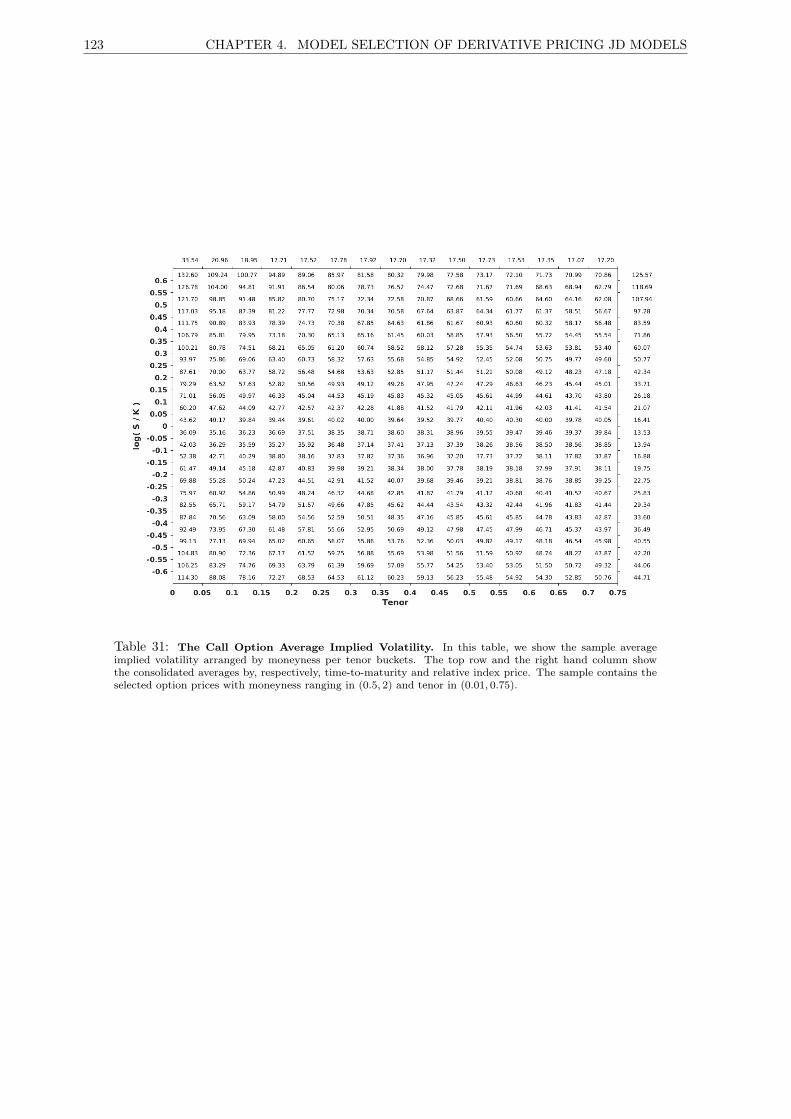
123 CHAPTER 4. MODEL SELECTION OF DERIVATIVE PRICING JD MODELS
.
Table 31: The Call Option Average Implied Volatility. In this table, we show the sample averageimplied volatility arranged by moneyness per tenor buckets. The top row and the right hand column showthe consolidated averages by, respectively, time-to-maturity and relative index price. The sample contains theselected option prices with moneyness ranging in (0.5, 2) and tenor in (0.01, 0.75).

TABLES 124
Table 32: The Put Option Average Implied Volatility. In this table, we show the sample averageimplied volatility arranged by moneyness per tenor buckets. The top row and the right hand column showthe consolidated averages by, respectively, time-to-maturity and relative index price. The sample contains theselected option prices with moneyness ranging in (0.5, 2) and tenor in (0.01, 0.75).

125 CHAPTER 4. MODEL SELECTION OF DERIVATIVE PRICING JD MODELS
Table 33: The Call Option Data Distribution. In this table, we show the sample data distributionarranged by moneyness per tenor buckets. The top row and the right hand column show the consolidatedweights by, respectively, time-to-maturity and relative index price.
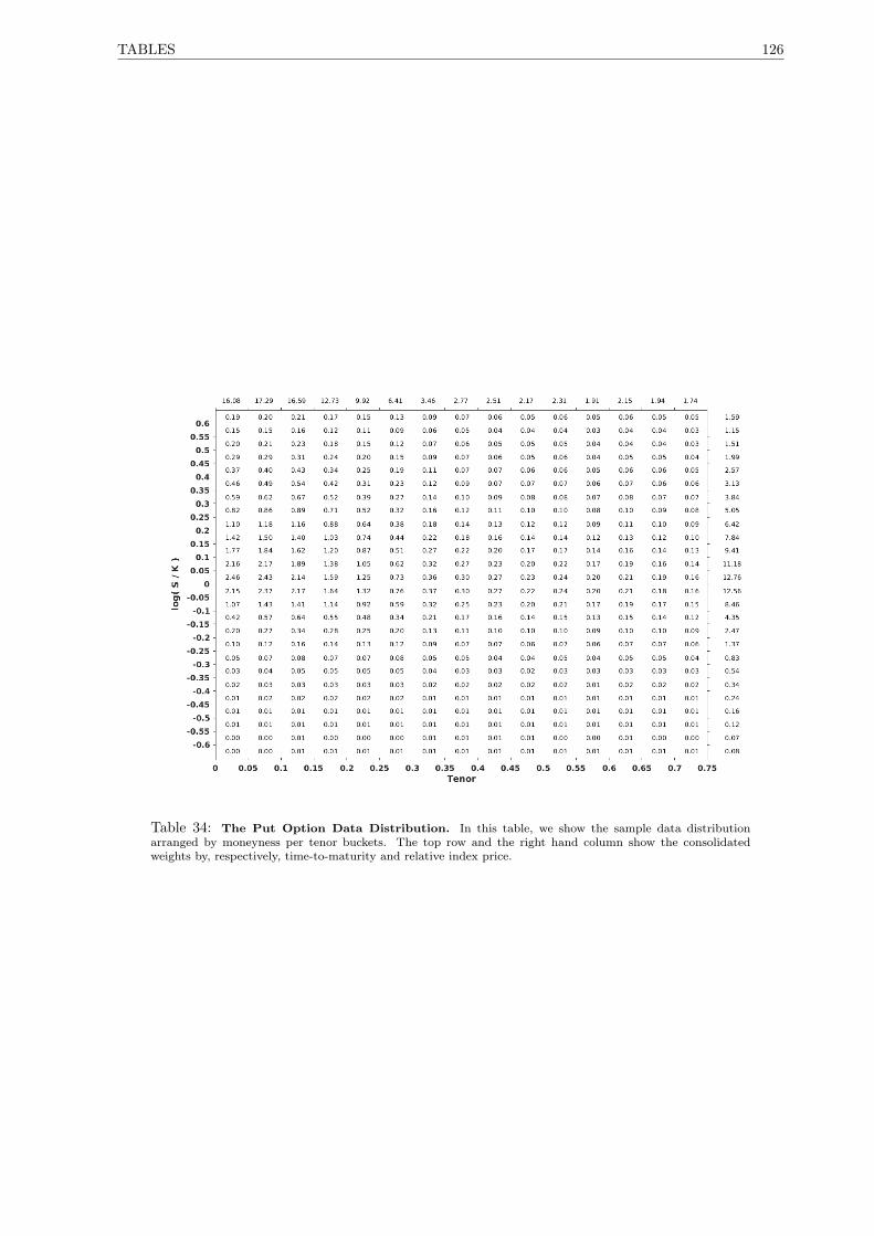
TABLES 126
Table 34: The Put Option Data Distribution. In this table, we show the sample data distributionarranged by moneyness per tenor buckets. The top row and the right hand column show the consolidatedweights by, respectively, time-to-maturity and relative index price.
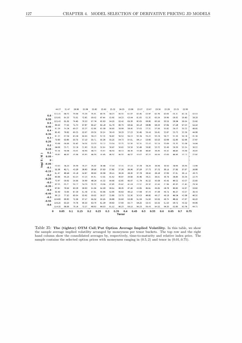
127 CHAPTER 4. MODEL SELECTION OF DERIVATIVE PRICING JD MODELS
Table 35: The (tighter) OTM Call/Put Option Average Implied Volatility. In this table, we showthe sample average implied volatility arranged by moneyness per tenor buckets. The top row and the righthand column show the consolidated averages by, respectively, time-to-maturity and relative index price. Thesample contains the selected option prices with moneyness ranging in (0.5, 2) and tenor in (0.01, 0.75).
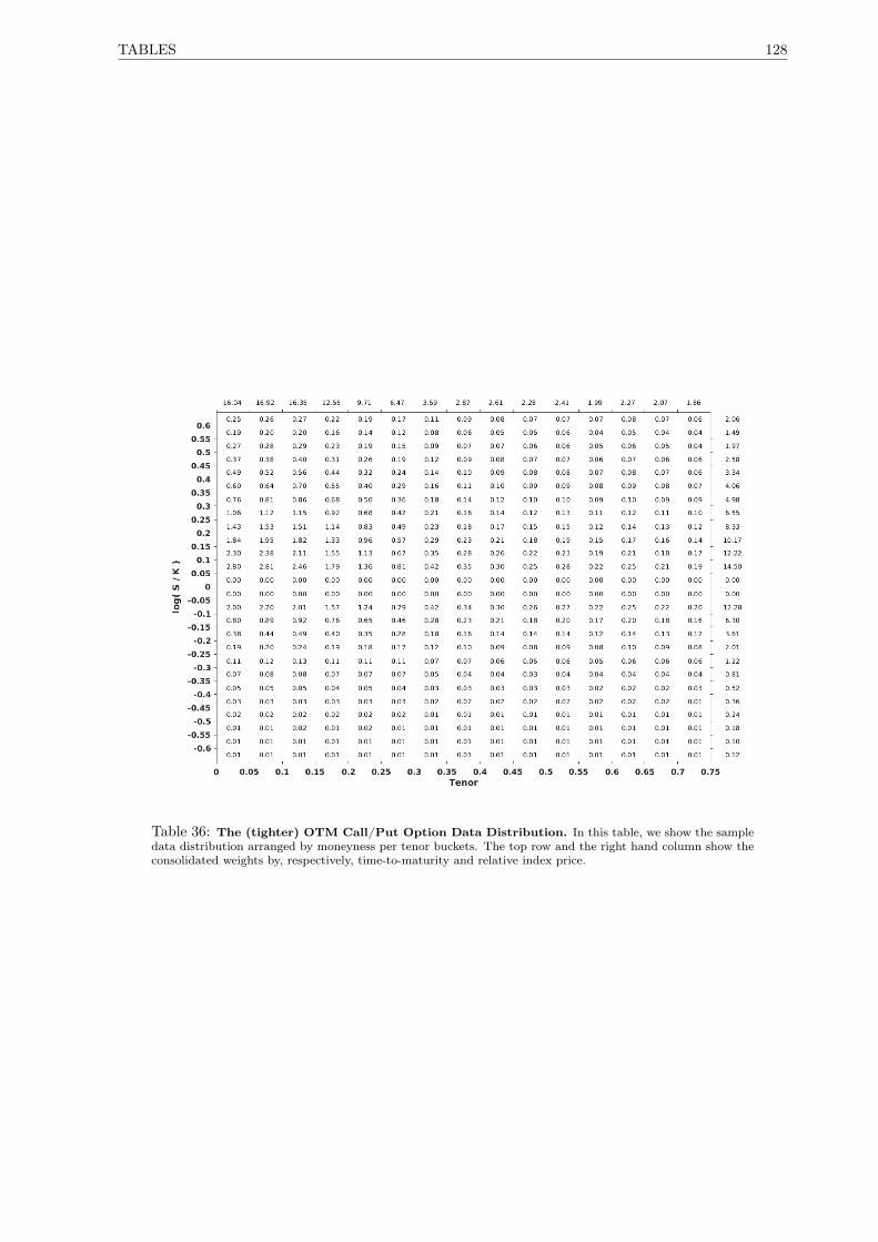
TABLES 128
Table 36: The (tighter) OTM Call/Put Option Data Distribution. In this table, we show the sampledata distribution arranged by moneyness per tenor buckets. The top row and the right hand column show theconsolidated weights by, respectively, time-to-maturity and relative index price.

129 CHAPTER 4. MODEL SELECTION OF DERIVATIVE PRICING JD MODELS
Bootstrap MCS-γOTM sample γ = 20% OTM sample γ = 40% ALL sample γ = 20% ALL sample γ = 40%
ZVR1XJE2 0.7791 ZVR1XJE2 0.6235 LZR1XJE1 0.8220 LZR1XJE1 0.6053ZZR1XJE2 0.7468 ZZR1XJE2 0.6032 ZZR1XJE1 0.8154 ZZR1XJE1 0.3947ZVR1CJ 0.7140 ZVR1XJN1 0.4498 LZR1JJE1 0.7925ZVR1XJN1 0.6536 ZVR1XJE1 0.4217 LVR1XJE1 0.7214ZVR1XJL2 0.6447 ZVR1XJL2 0.4018 LVR1XJEE 0.7051ZVR1XJE1 0.6407 ZVR1XJEE 0.6906ZVR1XJL1 0.4878 LVR1JJE1 0.6488ZZR1XJL1 0.4841 LZR1JJL1 0.5984LVR1XJEE 0.4817 ZZR1JJLL 0.5801ZVR1XJN0 0.4592 LZR0XJEE 0.5590ZZR0XJE2 0.4519 LZR1XJEE 0.5515LZR0XJE2 0.4416 LZR1JJLL 0.5503LVR1XJE2 0.4356 LZR0XJN1 0.5391ZZR1XJLL 0.4153 ZZR1XJLL 0.5297ZVR1 0.3868 LZR1XJLL 0.5204ZZR1XJL2 0.3861 LZR0XJE1 0.5144CVR1CJ 0.3637 LZR0JJE1 0.4963ZZR1XJN0 0.2904 LZR1XJL1 0.4954LVR1XJLL 0.2368 ZZR1XJL1 0.4952
LVR1XJLL 0.4767ZZR0XJE1 0.4606ZZR1XJEE 0.4562LZR0JJN1 0.4547ZZR0XJEE 0.4524ZVR1JJLL 0.3996LVR1JJL1 0.3879ZVR1JJL1 0.3672ZVR1XJLL 0.3596ZVR1XJL1 0.3356LVR1XJL1 0.2798LVR1JJLL 0.2678CSR1XJLL 0.2554CSR1XJL1 0.2354CSR1XJEE 0.1855
Table 37: Bootstrap MCS-γ fix at 20% and 40% OTM and ALL sample. In this table, we present theMCS results for the model selection of the OTM and ALL sample estimated option pricing model experiment,exploiting the MCS-γ with fixed k-FWER at 20% and 40% of the total number of comparisons. When comparedwith the following Tab. 38 with respect to the ALL sample, it is evident how the novel MHT based MCS test iscapable of a more selective results, which can be modulated by targeting the k family-wise error rate. The mainresult ofthe analysis is represented by the rejection of the affine family, which does not produce any equivalentperformance to the best MCS. It also worth to notice the performance of a simplified model, such as the ZVR1,that is the diffusive log-normal volatility model, which enters the restricted MCS for the OTM sample. Simpleaugmentations to this model, such as a single directional jump, as in the ZVR1XJE1 in the latter sample, or thestochastic intensity in the ALL sample (an extension that does not include further parameters) produce one ofthe top models.
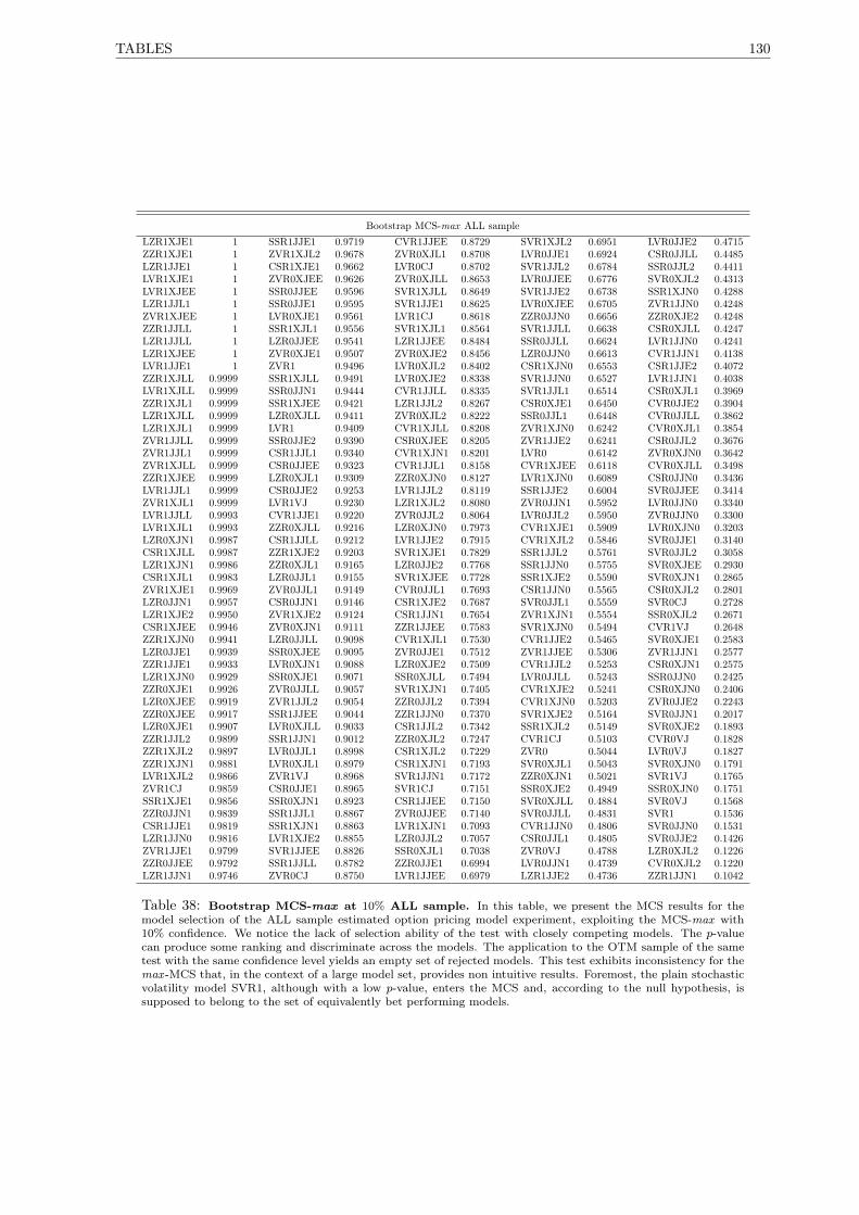
TABLES 130
Bootstrap MCS-max ALL sampleLZR1XJE1 1 SSR1JJE1 0.9719 CVR1JJEE 0.8729 SVR1XJL2 0.6951 LVR0JJE2 0.4715ZZR1XJE1 1 ZVR1XJL2 0.9678 ZVR0XJL1 0.8708 LVR0JJE1 0.6924 CSR0JJLL 0.4485LZR1JJE1 1 CSR1XJE1 0.9662 LVR0CJ 0.8702 SVR1JJL2 0.6784 SSR0JJL2 0.4411LVR1XJE1 1 ZVR0XJEE 0.9626 ZVR0XJLL 0.8653 LVR0JJEE 0.6776 SVR0XJL2 0.4313LVR1XJEE 1 SSR0JJEE 0.9596 SVR1XJLL 0.8649 SVR1JJE2 0.6738 SSR1XJN0 0.4288LZR1JJL1 1 SSR0JJE1 0.9595 SVR1JJE1 0.8625 LVR0XJEE 0.6705 ZVR1JJN0 0.4248ZVR1XJEE 1 LVR0XJE1 0.9561 LVR1CJ 0.8618 ZZR0JJN0 0.6656 ZZR0XJE2 0.4248ZZR1JJLL 1 SSR1XJL1 0.9556 SVR1XJL1 0.8564 SVR1JJLL 0.6638 CSR0XJLL 0.4247LZR1JJLL 1 LZR0JJEE 0.9541 LZR1JJEE 0.8484 SSR0JJLL 0.6624 LVR1JJN0 0.4241LZR1XJEE 1 ZVR0XJE1 0.9507 ZVR0XJE2 0.8456 LZR0JJN0 0.6613 CVR1JJN1 0.4138LVR1JJE1 1 ZVR1 0.9496 LVR0XJL2 0.8402 CSR1XJN0 0.6553 CSR1JJE2 0.4072ZZR1XJLL 0.9999 SSR1XJLL 0.9491 LVR0XJE2 0.8338 SVR1JJN0 0.6527 LVR1JJN1 0.4038LVR1XJLL 0.9999 SSR0JJN1 0.9444 CVR1JJLL 0.8335 SVR1JJL1 0.6514 CSR0XJL1 0.3969ZZR1XJL1 0.9999 SSR1XJEE 0.9421 LZR1JJL2 0.8267 CSR0XJE1 0.6450 CVR0JJE2 0.3904LZR1XJLL 0.9999 LZR0XJLL 0.9411 ZVR0XJL2 0.8222 SSR0JJL1 0.6448 CVR0JJLL 0.3862LZR1XJL1 0.9999 LVR1 0.9409 CVR1XJLL 0.8208 ZVR1XJN0 0.6242 CVR0XJL1 0.3854ZVR1JJLL 0.9999 SSR0JJE2 0.9390 CSR0XJEE 0.8205 ZVR1JJE2 0.6241 CSR0JJL2 0.3676ZVR1JJL1 0.9999 CSR1JJL1 0.9340 CVR1XJN1 0.8201 LVR0 0.6142 ZVR0XJN0 0.3642ZVR1XJLL 0.9999 CSR0JJEE 0.9323 CVR1JJL1 0.8158 CVR1XJEE 0.6118 CVR0XJLL 0.3498ZZR1XJEE 0.9999 LZR0XJL1 0.9309 ZZR0XJN0 0.8127 LVR1XJN0 0.6089 CSR0JJN0 0.3436LVR1JJL1 0.9999 CSR0JJE2 0.9253 LVR1JJL2 0.8119 SSR1JJE2 0.6004 SVR0JJEE 0.3414ZVR1XJL1 0.9999 LVR1VJ 0.9230 LZR1XJL2 0.8080 ZVR0JJN1 0.5952 LVR0JJN0 0.3340LVR1JJLL 0.9993 CVR1JJE1 0.9220 ZVR0JJL2 0.8064 LVR0JJL2 0.5950 ZVR0JJN0 0.3300LVR1XJL1 0.9993 ZZR0XJLL 0.9216 LZR0XJN0 0.7973 CVR1XJE1 0.5909 LVR0XJN0 0.3203LZR0XJN1 0.9987 CSR1JJLL 0.9212 LVR1JJE2 0.7915 CVR1XJL2 0.5846 SVR0JJE1 0.3140CSR1XJLL 0.9987 ZZR1XJE2 0.9203 SVR1XJE1 0.7829 SSR1JJL2 0.5761 SVR0JJL2 0.3058LZR1XJN1 0.9986 ZZR0XJL1 0.9165 LZR0JJE2 0.7768 SSR1JJN0 0.5755 SVR0XJEE 0.2930CSR1XJL1 0.9983 LZR0JJL1 0.9155 SVR1XJEE 0.7728 SSR1XJE2 0.5590 SVR0XJN1 0.2865ZVR1XJE1 0.9969 ZVR0JJL1 0.9149 CVR0JJL1 0.7693 CSR1JJN0 0.5565 CSR0XJL2 0.2801LZR0JJN1 0.9957 CSR0JJN1 0.9146 CSR1XJE2 0.7687 SVR0JJL1 0.5559 SVR0CJ 0.2728LZR1XJE2 0.9950 ZVR1XJE2 0.9124 CSR1JJN1 0.7654 ZVR1XJN1 0.5554 SSR0XJL2 0.2671CSR1XJEE 0.9946 ZVR0XJN1 0.9111 ZZR1JJEE 0.7583 SVR1XJN0 0.5494 CVR1VJ 0.2648ZZR1XJN0 0.9941 LZR0JJLL 0.9098 CVR1XJL1 0.7530 CVR1JJE2 0.5465 SVR0XJE1 0.2583LZR0JJE1 0.9939 SSR0XJEE 0.9095 ZVR0JJE1 0.7512 ZVR1JJEE 0.5306 ZVR1JJN1 0.2577ZZR1JJE1 0.9933 LVR0XJN1 0.9088 LZR0XJE2 0.7509 CVR1JJL2 0.5253 CSR0XJN1 0.2575LZR1XJN0 0.9929 SSR0XJE1 0.9071 SSR0XJLL 0.7494 LVR0JJLL 0.5243 SSR0JJN0 0.2425ZZR0XJE1 0.9926 ZVR0JJLL 0.9057 SVR1XJN1 0.7405 CVR1XJE2 0.5241 CSR0XJN0 0.2406LZR0XJEE 0.9919 ZVR1JJL2 0.9054 ZZR0JJL2 0.7394 CVR1XJN0 0.5203 ZVR0JJE2 0.2243ZZR0XJEE 0.9917 SSR1JJEE 0.9044 ZZR1JJN0 0.7370 SVR1XJE2 0.5164 SVR0JJN1 0.2017LZR0XJE1 0.9907 LVR0XJLL 0.9033 CSR1JJL2 0.7342 SSR1XJL2 0.5149 SVR0XJE2 0.1893ZZR1JJL2 0.9899 SSR1JJN1 0.9012 ZZR0XJL2 0.7247 CVR1CJ 0.5103 CVR0VJ 0.1828ZZR1XJL2 0.9897 LVR0JJL1 0.8998 CSR1XJL2 0.7229 ZVR0 0.5044 LVR0VJ 0.1827ZZR1XJN1 0.9881 LVR0XJL1 0.8979 CSR1XJN1 0.7193 SVR0XJL1 0.5043 SVR0XJN0 0.1791LVR1XJL2 0.9866 ZVR1VJ 0.8968 SVR1JJN1 0.7172 ZZR0XJN1 0.5021 SVR1VJ 0.1765ZVR1CJ 0.9859 CSR0JJE1 0.8965 SVR1CJ 0.7151 SSR0XJE2 0.4949 SSR0XJN0 0.1751SSR1XJE1 0.9856 SSR0XJN1 0.8923 CSR1JJEE 0.7150 SVR0XJLL 0.4884 SVR0VJ 0.1568ZZR0JJN1 0.9839 SSR1JJL1 0.8867 ZVR0JJEE 0.7140 SVR0JJLL 0.4831 SVR1 0.1536CSR1JJE1 0.9819 SSR1XJN1 0.8863 LVR1XJN1 0.7093 CVR1JJN0 0.4806 SVR0JJN0 0.1531LZR1JJN0 0.9816 LVR1XJE2 0.8855 LZR0JJL2 0.7057 CSR0JJL1 0.4805 SVR0JJE2 0.1426ZVR1JJE1 0.9799 SVR1JJEE 0.8826 SSR0XJL1 0.7038 ZVR0VJ 0.4788 LZR0XJL2 0.1226ZZR0JJEE 0.9792 SSR1JJLL 0.8782 ZZR0JJE1 0.6994 LVR0JJN1 0.4739 CVR0XJL2 0.1220LZR1JJN1 0.9746 ZVR0CJ 0.8750 LVR1JJEE 0.6979 LZR1JJE2 0.4736 ZZR1JJN1 0.1042
Table 38: Bootstrap MCS-max at 10% ALL sample. In this table, we present the MCS results for themodel selection of the ALL sample estimated option pricing model experiment, exploiting the MCS-max with10% confidence. We notice the lack of selection ability of the test with closely competing models. The p-valuecan produce some ranking and discriminate across the models. The application to the OTM sample of the sametest with the same confidence level yields an empty set of rejected models. This test exhibits inconsistency for themax -MCS that, in the context of a large model set, provides non intuitive results. Foremost, the plain stochasticvolatility model SVR1, although with a low p-value, enters the MCS and, according to the null hypothesis, issupposed to belong to the set of equivalently bet performing models.
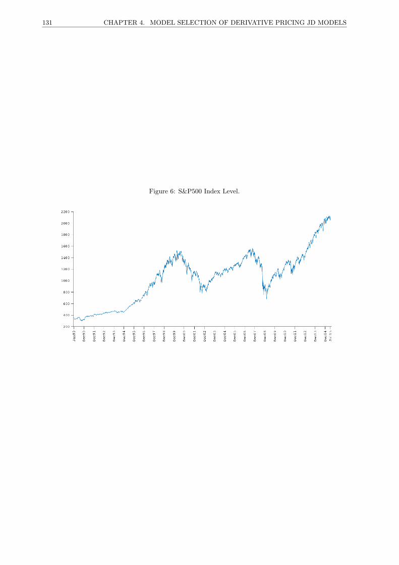
131 CHAPTER 4. MODEL SELECTION OF DERIVATIVE PRICING JD MODELS
.
Figure 6: S&P500 Index Level.

FIGURES 132
Figure 7: Put/Call Parity Distribution.
The figure shows the event counting of the Put/Call parity of the full option sample, after the cut-off of the 5-97.5percentile tails. We notice the quite wide range of variation of the relative price unbalance, which appears to bemore concentrated on the negative tail.

133 CHAPTER 4. MODEL SELECTION OF DERIVATIVE PRICING JD MODELS
Figure 8: The Selection of the Option Price Sample.
The figure shows the option price sample before and after the data selection, implemented by dropping the optionpairs displaying extreme put/call parity behaviour. A marginal data point selection has been achieved via visualinspection. The charts shows, proceeding from the top to the bottom, the call option sample (blue points) beforeand after the selection, plotted on the x axis showing the difference between the actual index level and the strike,irrespective of the time-to-maturity dimension. The put option sample (red points) before and after the selectionare exhibited at the bottom of the chart.
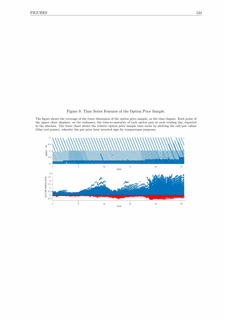
FIGURES 134
Figure 9: Time Series Features of the Option Price Sample.
The figure shows the coverage of the tenor dimension of the option price sample, as the time elapses. Each point ofthe upper chart displays, on the ordinates, the time-to-maturity of each option pair at each trading day, reportedin the abscissa. The lower chart shows the relative option price sample time series by plotting the call/put values(blue/red points), whereby the put price have inverted sign for compactness purposes.

135 CHAPTER 4. MODEL SELECTION OF DERIVATIVE PRICING JD MODELS
Figure 10: The RMSE Time Series.
The figure shows the average across the models of the daily RMSE in percentage obtained from the interpolationof the option pricing function over the ALL option sample. The red dots represents the daily min and max RMSEacross the model sample data. There seems to be a visible pattern of the model RMSE, starting from the late 90’s,whereby the dispersion of the RMSE appears to have shrunk. We conjecture that either the quality of the averagemodel has improved, implying less and less price outliers, or more simply, the range of the traded options has grownin such a way that the average RMSE has reduced, although larger pricing error might be concentrated on certainareas of the moneyness/maturity domain.
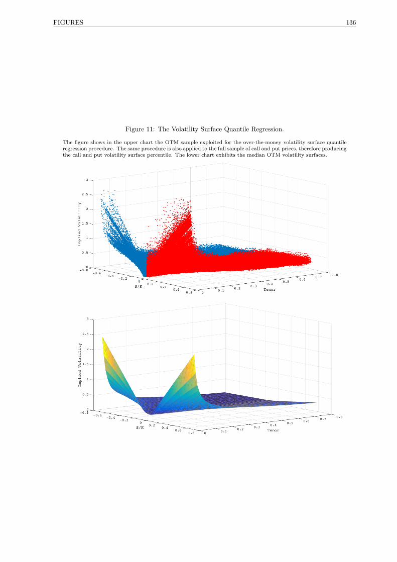
FIGURES 136
Figure 11: The Volatility Surface Quantile Regression.
The figure shows in the upper chart the OTM sample exploited for the over-the-money volatility surface quantileregression procedure. The same procedure is also applied to the full sample of call and put prices, therefore producingthe call and put volatility surface percentile. The lower chart exhibits the median OTM volatility surfaces.

137 CONCLUSIONS
Conclusions
In this thesis, we have presented several applications of the generalised MHT approach of Romano and
Wolf (2005a, 2007, 2010), providing a statistical method to confront the problem of model selection in a
very general setting. The experimental exercises that have been conducted, provide an example of the
flexibility and ease of implementation of the proposed tests. Disregarding the complexity of the problem,
the procedure requires only bootstrap samples of the target model performance measures and is capable
of delivering tests of significance, tests of benchmark comparison (relative model performance) and tests
for the automatic selection of the equivalently best performing models (absolute model performance), the
latter achieved with the support of the MCS construction (Hansen et al., 2011). In Chapter 2, we have
designed tests of model performance statistical significance with the balanced confidence set introduced
in the seminal work of Beran (1988a,b, 1990) and generalised in the reference work of Romano and oth-
ers, further augmented with the step-down method of Romano and Wolf (2005a, 2007) and Romano and
Shaikh (2006), an MHT procedure that allows to increase the power of the test. In a particular exper-
iment of Chapter 3, we have utilised the concept of model comparison via a loss function implemented
in studies such as Diebold and Mariano (1995), West (1996) to derive relative model comparison tests
targeting a benchmark model, in a context similar to the reality check of White (2000) and the superior

CONCLUSIONS 138
predictive ability test of Hansen (2005). Despite the similarity with the objective of these tests, our con-
tribution is original in that we have designed relative performance tests within the MHT framework that
not only test the hypothesis of models being superior to the benchmark, but that are otherwise capable of
identifying the subsets of superior, equivalent and inferior models such to partition the initial set into the
corresponding collections of superior, equivalent and inferior models. Comparable explicit results have
previously been obtained, within the context of MHT, in the article of Romano and Wolf (2005b). When
the structure of the problem permits the exploitation of the relative performance test, the inference is
delivered by a single instance of the procedure, as in the simulated experiment of Section 3.3.2. Alter-
natively, when a benchmark is not identifiable or even unnecessary, we have experimented the use of the
relative performance test by circulating the benchmark model across the model set, as executed in the
first part of Section 3.3.3. This approach has the benefit of exposing the complete pairwise contrasting of
the models belonging to the initial model set, but otherwise providing an excess of information that can
be synthesised into a model selection decision only through a careful and, to a certain extent, subjective
process of consideration. With this regard, in this thesis we have provided a significant further contribu-
tion to the literature by assembling a model selection procedure for the automatic detection of the set of
superior models, which inherits all the properties of the generalised MHT. In the Chapter 2, Chapter 3
and Chapter 4, we have built on the MCS concept introduced by the seminal work of Hansen et al. (2011),
as defined in (1.3.1), and designed absolute model performance tests. This procedure is represented by
the γ-MCS of Section 1.3.3, an MHT that regards the model selection as a multi-dimensional test in-
volving hypotheses of model superiority on the full set of pairwise model comparisons, which eventually
filters those accepted hypotheses with the application of the MCS rule. As a term of reference, we have
constructed the established MCS test of the cited authors with the implementation of the max -MCS
as in Section 1.3.1, which delivers also a p-value model ranking measure that is based on the sequence
of the p-values of the target statistic. On the contrary, the model ranking measure associated to our
novel test builds on the multidimensional statistic bootstrap distribution and provides an estimate of
the probability that each model in the model set be superior to any element belonging to the MCS.
As a complementary exercise, we have also included a streamlined MCS test version by modifying and
adapting the approach in Corradi and Distaso (2011), a method that disregards test dependencies and
the control of the k-FWER, as presented in Section 1.3.2. This test displays some affinity with the
γ-MCS, in that it potentially explores the full combination of model comparisons, but instead ignores
the hypotheses structure relaying on scalar asymptotic tests for the implementation of the preference
decision rule. We have indicated this test as the t-MCS. The model ranking measure delivered by the
t-MCS is defined by taking the worst expected relative performance for each model as determined by
the bootstrap method and computing the complement of its quantile on a standard normal distribution,
that is the worst p-value for each model with respect to any model comparison. The observation of the
experimental results highlights the importance of the MHT paradigm, which in situations whereby the
model selection is problematic, allows to modulate between some conservative results, such those provided
by the max -MCS and some other boundary outcomes, such those provided by the t-MCS, which tends
to strongly restrict the MCS. With this research, we have been studying procedures that allow flexibility
of usage, preserving robustness and rigour of the analysis. As a result, the model selection procedures
that we have presented have the merit of reducing the main research question to a problem of exper-

139 CONCLUSIONS
imental design, leaving to the investigator the task of the construction of the model performance measure.
In the course of the experimental exercises, we have explored and provided significant evidence concern-
ing several problems in financial econometrics involving the decision as to which model is preferable for
a given task. We have analysed three typical prototype problems in investment portfolios exposed to
market risk, that is the estimation of several portfolio risk metrics such as the VaR and the ExS, as well
as the estimation of the historical and the risk-neutral measures of widely employed stochastic processes
in finance, such as JD models. In Chapter 2 we have dealt with market risk model selection. Targeting
model performance measures of VaR and ExS, we have constructed statistical significance MHT and
absolute model performance test. The model set contains a small but very diverse collection of market
risk forecasting model. We have obtained results that diverge from the precedent analysis of Bao et al.
(2006), whose general conclusion consists in the lack of a superior model in the relative performance
contest, whereby the benchmark model is represented by the RiskMetrics model. On the contrary, we
provide evidence that some of the GARCH models and to a certain extent the quantile regression models,
provide the best performance on the short term horizon, whereas on the longer forecast horizon the MCS
is very wide and the model ranking measure only can provide some indications. In Chapter 3, we have
tackled the estimation of JD models under the historical measure. We have produced an original model
selection exercise involving affine models with jump extensions, as well as stochastic intensity models with
high frequency jumps. The analysis of this chapter has targeted measures of likelihood and of filtering
performance. With the market data experiment, we have obtained evidence confirming the findings of
Jones (2003) in relation to the superiority of the CEV extension with respect to the plain affine stochastic
volatility model, as well as highlighting the importance of jumps in returns, as in Andersen et al. (2002),
Chernov et al. (2003) and Eraker et al. (2003). Furthermore, the analysis of MCS tests has rejected the
inclusion of a jump in the volatility factor, providing an element of model simplification, as opposed to
the result of Eraker et al. (2003) and more in line with what has been remarked in Chernov et al. (2003),
although the results of our test concerning the jump in volatility component are more explicit. Another
interesting result of the market data experiment pointed out the excellent performance of some SH mod-
els, providing indication for a slightly more parsimonious parametrisation. Finally, with the Chapter 4,
we have explored model selection from a very large JD option pricing model set. The analysis of this
chapter has targeted a measure of RMSE. The particularly large model set and the extreme similarity
of the model performances have caused troubles to the max -MCS, which has not been able to discrim-
inate across the competitors collection. In this exercise the flexibility of our novel γ-MCS has revealed
a substantial advantage. Moreover, the tests have provided indication of the superiority of the exponen-
tial stochastic volatility model, a result in line with the findings of Christoffersen et al. (2010), whereby
models producing high kurtosis and large spikes in the volatility factor are preferable. The results of our
tests also points to a containment of the complexity of the model.
As a further contribution to the literature of this thesis, in Chapter 2 we have produced a novel ExS test
and in Chapter 3 we have extended the nonlinear filter of Maybeck (1982) with a jump component.
With regards to a thorough comparison of the model selection tests employed in this thesis, we remark

CONCLUSIONS 140
that such a task is beyond the scope of the work. However, from a theoretical standpoint, we notice the
following. Foremost, we are inclined to prefer the γ-MCS as the max -MCS lacks of control for the gener-
alised FWER, whereby in a context such that the number of tests in the MHT is remarkable, the control
of the mere FWER becomes too stringent. Moreover, the γ-MCS, hinging on the MHT approach, it
grants the strong control of the k-FWER. In more practical terms regarding the confrontation of the dif-
ferent tests, we have collected evidence that allows qualitative comparison. We have encountered diverse
circumstances, whereby the max -MCS and the γ-MCS tend to perform similarly in a context whereby
the best models are unambiguously identified, such as the 1d market risk metrics forecast experiment
in Chapter 2 and the LRMCS test of the market data experiment in Chapter 3, whereas the t-MCS
produces smaller top model sets. We notice moreover that, as it allows for the control of the generalised
FWER, the MHT based MCS offers a gear to modulate the sensitivity to false rejections and hence
identify models that are close to rejection, further contracting the MCS. Under conditions whereby the
model comparison is more ambiguous and all of the MCS tests struggle to identify the best model set, as
it is the case of the 2w forecasting exercise of Chapter 2 and the simulation experiment involving model
aliasing of Chapter 3, the γ-MCS provides a more informative model ranking measure, while the t-MCS
results in a tighter selection. The latter test might be useful as a quick diagnostic tool to identify the
region containing the candidate best models or in conditions where it is difficult to distinguish models,
the t-MCS might provide a term of comparison for various γ values in the γ-MCS. In the final model
selection exercise of Chapter 4, we deal with a very large model set, whereby the ability of the γ-MCS to
modulate the result by targeting different k-FWER allows one to focus upon the set of best performing
models, whereas the benchmark test max -MCS is incapable of providing any insight as for the best model
set out of the initial pool. A further term of comparison can be identified in the behaviour of the p-value,
that in the case of the max -MCS exhibits the tendency for a lack of discriminating capacity between the
top section of the MCS components. Eventually, the p-value model ranking measure that we construct
for our novel test, provides a highly significant ranking factor. In conclusion, the model selection tests we
develop and apply in this research constitute an approach that is very promising in providing important
support in problems of model risk.
For the future research, we expect the refinement of the core procedures and plan to extend the study
of the theoretical properties of the max -MCS and the γ-MCS and how they relate each other and they
relate to a test such as the t-MCS. Moreover, the many algorithms that have been studied and developed
in this research provide further matter for extensions and application to financial econometric problems
such as market risk, filtering, likelihood estimation and pricing. Finally, we notice that particularly in
the context of JD models, the uncertainty related to the parameters estimation is considerable and hence
further research in this domain aiming at producing applications in the model risk space is attractive. In
particular, a topic of interest is the measurement of the model risk associated to parameter uncertainty.
Further analysis can be conducted in the domain of model transformations that simplify the computation
procedures and reduce the estimation risk. Moreover, we notice that the analysis in Chapter 3 is partial to
a certain extent, as it lacks further testing in term of loss measures targeting specifically the distribution
tails, and the analysis would benefit from an extension of the likelihood to a full Bayesian approach.
As a notice for future research in relation to Chapter 4, a limitation of this study consists of the lack

141 CONCLUSIONS
of analysis such as the coherence of the implied factor distributions generated by market prices or the
hedging performance of the model set such as, for instance, in Bakshi et al. (1997), Bates (2000). Further
directions of future research might concern the derivation of statistical arbitrage strategies through the
analysis of the dynamics of the mispricing error or that of the premium to a replicating portfolio strategy.
Another important insight, which has been suggested by the examiners, consists of exploring the model
ranking through time to highlight possible patterns in the evolution of the pricing errors, which might
inform the construction of statistical arbitrage trading strategies.


143 BIBLIOGRAPHY
Bibliography
Aït-Sahalia, Y. (1996). Testing continuous-time models of the spot interest rate. Review of Financial
Studies, 9:385–426.
Aït-Sahalia, Y. (1999). Transition densities for interest rate and other nonlinear diffusions. Review of
Financial Studies, 54:1361–1395.
Aït-Sahalia, Y. (2002). Maximum likelihood estimation of discretely sampled diffusions: a closed-form
approximation approach. Econometrica, 70(1):223–262.
Aït-Sahalia, Y. (2004). Disentangling diffusion from jumps. Journal of Financial Economics, 74:487–528.
Aït-Sahalia, Y. (2008). Closed-form likelihood expansions for multivariate diffusions. The Annals of
Statistics, 36(2):906–937.
Aït-Sahalia, Y. and Kimmel, R. (2007). Maximum likelihood estimation of stochastic volatility models.
Journal of Financial Econometrics, 83:413–452.
Akaike, H. (1974). A new look at the statistical model identification. Automatic Control, IEEE Trans-
actions on Automatic Control, 19(6):716–723.
Akaike, H. (1981). Likelihood of a model and information criteria. Journal of Econometrics, 16(1):3–14.

BIBLIOGRAPHY 144
Andersen, T., Benzoni, L., and Lund, J. (2002). An empirical investigation of continuous time equity
return models. Journal of Finance, 57(3):1239–1284.
Artzner, P., Delbaen, P., Eber, J., and Heath, D. (1999). Coherent measures of risk. Mathematical
Finance, 9(3).
Baadsgaard, M., Nielsen, J., and Madsen, H. (2000). Estimating multivariate exponential-affine term
structure models from coupon bond prices using nonlinear filtering. Econometric Journal, 3:1–20.
Bakshi, G., Cao, C., and Chen, Z. (1997). Empirical performance of alternative option pricing models.
The Journal of Finance, 52(5):2003–2049.
Bakshi, G., Ju, N., and Ou-Yang, H. (2006). Estimation of continuous-time models with an application
to equity volatility dynamics. Journal of Financial Economics, 82(1):227–249.
Bao, Y., Lee, T., and Saltoğlu, B. (2006). Evaluating predictive performance of Value-at-Risk models in
emerging markets: A reality check. Journal of Forecasting, 25.
Bao, Y., Lee, T., and Saltoğlu, B. (2007). Comparing density forecast models. Journal of Forecasting,
26.
Barndorff-Nielsen, O. and Shephard, N. (2002). Econometric analysis of realized volatility and its use in
estimating stochastic volatility models. Journal of the Royal Statistical Society: Series B (Statistical
Methodology), 64(2):253–280.
Barndorff-Nielsen, O. and Shephard, N. (2004). Power and bipower variation with stochastic volatility
and jumps. Journal of Financial Econometrics, 2(1):1–37.
Basel Committee on Banking Supervision (2009). Supervisory guidance for assessing banks’ financial
instrument fair value practices. Technical report, Bank for International Settlements.
Bates, D. (1996). Jumps and stochastic volatility: exchange rate processes implied in deutsche mark
options. Review of Financial Studies, 9:69–107.
Bates, D. (2000). Post-’87 crash fears in the S&P 500 futures option market. Journal of Econometrics,
94(1-2):181–238.
Beckers, S. (1980). The constant elasticity of variance model and its implications for option pricing.
Journal of Finance, 35(3):661–73.
Benjamini, Y. and Hochberg, Y. (1995). Controlling the false discovery rate: a practical and powerful
approach to multiple testing. Journal of the Royal Statistical Society, B, 57(1):289–300.
Benjamini, Y. and Hochberg, Y. (2000). On the adaptive control of the false discovery rate in multiple
testing with independent statistics. Journal of Educational and Behavioural Statistics, 25(1):60–83.
Benzoni, L. (2002). Pricing options under stochastic volatility: An empirical investigation. Carlson
School of Management Working Paper.

145 BIBLIOGRAPHY
Beran, R. (1988a). Balanced simultaneous confidence sets. Journal of the American Statistical Associa-
tion, 83(403):679–686.
Beran, R. (1988b). Prepivoting test statistics: a bootstrap view of asymptotic refinements. Journal of
the American Statistical Association, 83(403):687–697.
Beran, R. (1990). Refining bootstrap simultaneous confidence sets. Journal of the American Statistical
Association, 85(410):417–426.
Beran, R. (2003). The impact of bootstrap on statistical algorithms and theory. Statistical Science,
18(2):175–184.
Berkowitz, J. (2001). Testing density forecasts with applications to risk management. Journal of Business
and Economic Statistics.
Bierens, H. (1987). Kernel estimators of regression functions. In Advances in Econometrics: Fifth World
Congress, volume 1. Palgrave, London.
BIS (2011). Messages from the academic literature on risk measurement for the trading book. Technical
Report 19, Bank for International Settlements.
Bollerslev, T. (1986). Generalized autoregressive conditional heteroskedasticity. Journal of Econometrics,
31(3):307–327.
Bollerslev, T. and Zhou, H. (2002). Estimating stochastic volatility diffusion using conditional moments
of integrated volatility. Journal of Econometrics, 109:33–65.
Breusch, T. S. and Pagan, A. (1980). The lagrange multiplier test and its applications to model specifi-
cation in econometrics. Review of Economic Studies, 47(1):239–253.
Carr, P. and Madan, D. (1999). Option valuation using the fast fourier transform. Journal of Computa-
tional Finance, 2:61–73.
Chako, G. and Viceira, L. (2003). Spectral GMM estimation of continuous-time processes. Journal of
Econometrics, 116:259–292.
Chernov, M., Gallant, A., Ghysels, E., and Tauchen, G. (2003). Alternative models of stock price
dynamics. Journal of Econometrics, 116:225–257.
Christoffersen, P. (1998). Evaluating interval forecasts. International Economic Review, 39.
Christoffersen, P., Dorion, C., Jacobs, K., and Karoui, L. (2014). Nonlinear kalman filtering in affine
term structure models. Technical Report 14-04, Centre Interuniversitaire sur le Risque, les Politiques
Èconomiques et l’Emploi.
Christoffersen, P., Jacobs, K., and Mimouni, K. (2010). Volatility dynamics for the s&p500: evidence
from realized volatility, daily returns, and option prices. Review of Financial Studies, 23(8):3141–3189.
Collin-Dufresne, P., Goldstein, R., and Jones, C. (2008). Identification of maximal affine term structure
models. Journal of Finance, 58(2):743–795.

BIBLIOGRAPHY 146
Cont, R. and Tankov, P. (2003). Financial modelling with jump processes. Chapman & Hall / CRC Press.
Corradi, V. and Distaso, W. (2011). Multiple forecast model evaluation. In The Oxford Handbook of
Economic Forecasting, chapter 13, pages 391–414. Oxford University Press.
Corradi, V. and Swanson, N. (2006). Bootstrap conditional distribution tests in the presence of dynamic
misspecification. Journal of Econometrics, 133(2):779–806.
Corradi, V. and Swanson, N. (2007). Non-parametric bootstrap procedures for predictive inference based
on recursive estimation schemes. International Economic Review, 48(1):67–109.
Cox, J. and Ross, S. (1976). The valuation of options for alternative stochastic processes. Journal of
Financial Economics, 3(1-2):145–166.
Cummins, M., Dowling, M., and Esposito, F. (2017). Determining risk model confidence sets. Finance
Research Letters, 21.
Dai, Q. and Singleton, K. (2000). Specification analysis of affine term structure models. Journal of
Finance, 55(5):1943–1978.
Dempster, M. and Tang, K. (2011). Estimating exponential affine models with correlated measurement
errors: applications to fixed income and commodities. Journal of Banking and Finance, 35:639–652.
Diebold, F. and Mariano, R. (1995). Comparing predictive accuracy. Journal of Business and Economic
Statistics, 13(3):253–263.
Diebold, F., Todd, A., and Tay, A. (1998). Evaluating density forecasts with applications to financial
risk management. International Economic Review.
Dotsis, G. and Markellos, R. N. (2008). An application of bootstrapping in option pricing. Technical
report, Athens University of Economics and Business.
Duffee, G. and Stanton, R. (2012). Estimation of dynamic term structure models. Quaterly Journal of
Finance, 2(2):1–51.
Duffie, D. and Kan, R. (1996). A yield factor model of interest rates. Mathematical Finance, 6(4):379–406.
Duffie, D., Pan, J., and Singleton, K. (2000). Trasform analysis and asset pricing for affine jump-diffusions.
Econometrica, 68(6):1343–1376.
Duffy, D. (2006). Finite difference methods in financial engineering: a partial differential equation ap-
proach. Wiley.
Durham, G. and Gallant, A. (2002). Numerical techniques for maximum likelihood estimation of
continuous-time diffusion processes. Journal of Business & Economic Statistics, 20(3):335–338.
Efron, B. (1979). Bootstrap methods: another look at the jackknife. The Annals of Statistics, 7(1):1–26.
Elerian, O., Chib, S., and Shephard, N. (2001). Likelihood inference for discretely observed nonlinear
diffusions. Econometrica, 69(4):959–993.

147 BIBLIOGRAPHY
Engle, R. (1982). Autoregressive conditional heteroscedasticity with estimates of the variance of united
kingdom inflation. Econometrica, 50(4):987–1007.
Engle, R. and Manganelli, S. (2004). CAViaR: Conditional autoregressive Value-at-Risk by regression
quantile. Journal of Business & Economic Statistics, 22(4):367–381.
Eraker, B. (2001). MCMC analysis of diffusion models with application to finance. The Journal of
Business & Economic Statistics, 19(2):177–191.
Eraker, B. (2004). Do stock prices and volatility jump? reconciling evidence from spot and option prices.
The Journal of Finance, 59(3):1367–1403.
Eraker, B., Johannes, M., and Polson, N. (2003). The impact of jumps in volatility and returns. The
Journal of Finance, 58(3):1269–1300.
Esposito, F. and Cummins, M. (2015). Multiple hypothesis testing of market risk forecasting models.
Working Paper.
Fisher, R. (1922). On the mathematical foundations of theoretical statistics. Philosophical Transactions
of the Royal Society of London A: Mathematical, Physical and Engineering Sciences, 222(594-604):309–
368.
Fisher, R. (1924). The conditions under which χ2 measures the discrepancy between observation and
hypothesis. Journal of the Royal Statistical Society, 87:442–450.
Gallant, A. and Tauchen, G. (1996). Which moments to match? Econometric Theory, 12(4):657–681.
Glosten, L., Jagannathan, R., and Runkle, D. (1993). On the relation between the expected value and
the volatility of the nominal excess return on stocks. Journal of Finance, 42(5):27–62.
Gonçalves, S. and White, H. (2002). The bootstrap of the mean for dependent heterogeneous arrays.
Econometric Theory, 18(6):1367–1384.
Gonzales-Rivera, G., Tae-Hwy, L., and Santosh, M. (2003). Forecasting volatility: A reality check based
on option pricing, utility functions, value-at-risk and predictive likelihood. Working Paper.
Gonzalo, J. and Olmo, J. (2004). Which extreme values are really extreme? Journal of Financial
Econometrics, 2(3).
Gordon, N., Salmond, D., and Smith, A. F. (1993). Novel approach to nonlinear/non-gaussian bayesian
state estimation. In IEE Proceedings F (Radar and Signal Processing), volume 140(2), pages 107–113.
Gupta, S. and Huang, D. (1976). Subset selection procedures for the means and variances of normal popu-
lations: unequal sample sizes case. Sankhya : The Indian Journal of Statistics, Series B, 38(2):112–128.
Hansen, P. (2005). A test for superior predictive ability. Journal of Business & Economic Statistics,
23(4):365–380.
Hansen, P. and Lunde, A. (2005). A forecast comparison of volatility models: does anything beat a
garch(1, 1)? Journal of Applied Econometrics, 20(7):873–889.

BIBLIOGRAPHY 148
Hansen, P., Lunde, A., and Nason, J. (2011). The model confidence set. Econometrica, 79(2):453–497.
Hanson, F. (2007). Applied stochastic processes and control for jump-diffusions: modelling, analysis, and
computation. Society for Industrial and Applied Mathematics.
Hausman, J. (1978). Specification tests in econometrics. Econometrica, 46(6):1251–71.
Heston, S. (1993). A closed-form solution for options with stochastic volatility with applications to bond
and currency options. The Review of Financial Studies, 6(2):327–343.
Holm, S. (1979). A simple sequentially rejective multiple test procedure. Scandinavian Journal of Statis-
tics, 6(2):65–70.
Horowitz, J. (2001). The Bootstrap. In Handbook of Econometrics, volume 5, chapter 52, pages 3159–
3228. Elsevier.
Hull, J. and White, A. (1987). The pricing of options on assets with stochastic volatilities. Journal of
Finance, 42(2):281–300.
Hurn, A., Lindsay, K., and McClelland, A. (2013). A quasi-maximum method for estimating the param-
eters of multivariate diffusions. Journal of Econometrics, 172:106–126.
Hurn, S., Jeisman, J., and Lindsay, K. (2010). Teaching an old dog new tricks: Improved estimation of
the parameters of stochastic differential equations by numerical solution of the fokker-planck equation.
In Financial Econometrics Handbook. Palgrave, London.
Hürzeler, M. and Künsch, H. (1998). Monte carlo approximations for general state-space models. Journal
of Computational and Graphical Statistics, 7(2):175–193.
Hwang, E. and Shin, D. (2012). Strong consistency of the stationary bootstrap under -weak dependence.
Statistics and Probability Letters, 82(3):488 – 495.
Jensen, B. and Poulsen, R. (2002). Transition densities of diffusion processes: numerical comparison of
approximation techniques. Journal of Derivatives, 9(4):18–30.
Johannes, M., Polson, N., and Stroud, J. (2009). Optimal filtering of jump diffusions: Extracting latent
states from asset prices. Review of Financial Studies, pages 2759–2799.
Jones, C. (1998). Bayesian estimation of continuous-time finance models. University of Rochester.
Jones, C. (2003). The dynamics of stochastic volatility: evidence from underlying and options markets.
Journal of econometrics, 116(1):181–224.
J.P.Morgan (1996). RiskmetricsTM . Technical Report 4, J.P.Morgan, Reuters.
Kerkhof, J. and Melenberg, B. (2003). Backtesting for risk-based regulatory capital. Working Paper.
Kerkhof, J., Melenberg, B., and Schumacher, H. (2009). Model risk and capital reserves. Working Paper.
Koenker, B. and Bassett, G. (1978). Regression quantiles. Econometrica, 46(1).
Kou, S. (2002). A jump-diffusion model for option pricing. Management Science, 48(8):1086–1011.

149 BIBLIOGRAPHY
Kou, S. and Wang, H. (2004). Option pricing under a double exponential jump diffusion model. Man-
agement Science, 50(9):1178–1192.
Kupiec, P. (1995). Techniques for verifying the accuracy of risk management models. Journal of Deriva-
tives, 3.
Küsch, H. (1989). The jackknife and the bootstrap for general stationary observations. The Annals of
Statistics, 17(3):1217–1241.
Lahiri, S. (1999). Theoretical comparisons of block bootstrap methods. The Annals of Statistics,
27(1):386–404.
Lindström, E. (2007). Estimating parameters in diffusion processes using an approximate maximum
likelihood approach. Annals of Operations Research, 151:269–288.
Linhart, H. (1988). A test whether two aic’s differ significantly. South African Statistical Journal,
22(2):153–161.
Liu, R. and Singh, K. (1992). Moving blocks jackknife and bootstrap capture weak dependence. In
Exploring the Limits of Bootstrap, pages 225–248. John Wiley & Sons.
Lo, A. (1988). Maximum likelihood estimation of Itô processes with discretely sampled data. Econometric
Theory, 4(2):231–247.
Longin, F. (1996). The asymptotic distribution of extreme stock market returns. The Journal of Business,
69.
Lund, J. (1997). Non-linear kalman filtering techniques for term structure models. Working Paper,
Aarhus School of Business.
Lux, T. (2012). Inference for systems of stochastic differential equations from discretely sampled data: a
numerical maximum likelihood approach. Technical Report 1781, Kiel Institute for the World Economy.
Macbeth, J. and Merville, L. (1980). Tests of black-scholes and cox call option valuation models. Journal
of Finance, 35(2):285–301.
Mancini, L. and Trojani, F. (2011). Robust value at risk prediction. The Journal of Financial Econo-
metrics, 9.
Marcus, R., Peritz, E., and Gabriel, K. (1976). On closed testing procedures with special reference to
ordered analysis of variance. Biometrika, 63(3):655–660.
Maybeck, P. (1982). Stochastic models, estimation and control, volume 2. Academic Press, London.
Merton, R. (1976). Option pricing when the underlying stock returns are discontinuous. Journal of
Financial Economics, 3:125–144.
Musiela, M. and Rutkowski, M. (1997). Martingale methods in financial modelling. Springer.
Nadaraya, E. (1964). On estimating regression. Theory of Probability and its Applications, 9.

BIBLIOGRAPHY 150
Nelson, D. (1991). Conditional heteroskedasticity in asset returns: A new approach. Econometrica,
59(2):347–370.
Newey, W. (1985). Maximum likelihood specification testing and conditional moment tests. Econometrica,
53(5):1047–70.
Nielsen, J., Vestgaard, M., and Madsen, H. (2000). Estimation in continuous-time stochastic volatility
models using nonlinear filters. International Journal of Theoretical and Applied Finance, 3(2):1–30.
Nordman, D. (2009). A note on the stationary bootstrap’s variance. The Annals of Statistics, 37(1):359–
370.
Office of the Comptroller of the Currency (2011). Supervisory guidance on model risk management.
Technical Report SR 11-7, Board of Governors of the Federal Reserve System.
Øksendal, B. (2003). Stochastic Differential Equations: An Introduction with Applications. Springer, 6
edition.
Pan, J. (2002). The jump-risk premia implicit in options: evidence from an integrated time-series study.
Journal of Financial Economics, 63(1):3–50.
Patton, A., Politis, D., and White, H. (2009). Correction to: Automatic block-length selection for
dependent bootstrap. Econometric Reviews, 28(4):372–375.
Pearson, K. (1936). Method of moments and method of maximum likelihood. Biometrika, 28(1/2):34–59.
Pedersen, A. (1995a). Consistency and asymptotic normality of an approximate maximum likelihood
estimator for discretely observed diffusion processes. Bernoulli, 1(3):257–279.
Pedersen, A. (1995b). A new approach to maximum likelihood estimation for stochastic differential
equations based on discrete observations. Board of the Foundation of the Scandinavian Journal of
Statistics, 22(1):57–71.
Perelló, J., Sircar, R., and Masoliver, J. (2008). Option pricing under stochastic volatility: the exponential
Ornstein−Uhlenbeck model. Journal of Statistical Mechanics: Theory and Experiment, 6:1–22.
Pitt, M. (2002). Smooth particle filters for likelihood evaluation and maximisation. University of Warwick,
Department of Economics.
Pitt, M. and Shephard, N. (1999). Filtering via simulation: Auxiliary particle filters. Journal of the
American statistical association, 94(446):590–599.
Platen, E. and Bruti-Liberati, N. (2010). Numerical solution of stochastic differential equations with
jumps in finance. Springer.
Politis, D. and Romano, J. (1994a). Limit theorems for weakly dependent hilbert space valued random
variables with applications to the stationary bootstrap. Statistica Sinica, 4(2):461–476.
Politis, D. and Romano, J. (1994b). The stationary bootstrap. Journal of the American Statistical
Association, 89(428):1303–1313.

151 BIBLIOGRAPHY
Politis, D. and White, H. (2004). Automatic block-length selection for dependent bootstrap. Econometric
Reviews, 23(1):53–70.
Poulsen, R. (1999). Approximate maximum likelihood estimation of discretely observed diffusion pro-
cesses. Technical Report 29, Centre for Analytical Finance, University of Aarhus.
Priestley, M. B. (1981). Spectral analysis and time series. Academic Press London ; New York.
Rao, C. and Wu, Y. (2001). On model selection. In Lahiri, P., editor, Model Selection, volume 38 of
Lecture notes - monograph series, chapter 1, pages 1–58. Institute of Maathematical Statistics.
Romano, J., Azeem, M., and Wolf, M. (2010). Hypothesis testing in econometrics. Annual Review of
Economics, 2:75–104.
Romano, J. and Shaikh, A. (2006). On stepdown control of the false discovery proportion, volume 49 of
Lecture Notes–Monograph Series, pages 33–50. Institute of Mathematical Statistics.
Romano, J., Shaikh, A., and Wolf, M. (2008). Formalized data snooping based on generalized error rates.
Econometric Theory, 24(2):404–447.
Romano, J. and Wolf, M. (2005a). Exact and approximate step-down methods for multiple hypothesis
testing. The Journal of the American Statistical Association, 100(469):94–108.
Romano, J. and Wolf, M. (2005b). Stepwise multiple testing as formalized data snooping. Econometrica,
73(4):1237–1282.
Romano, J. and Wolf, M. (2007). Control of generalized error rates in multiple testing. The Annals of
Statistics, 35(4):1378–1408.
Romano, J. and Wolf, M. (2010). Balanced control of generalized error rates. The Annals of Statistics,
38(1):598–633.
Rosenblatt, M. (1952). Remarks on a multivariate transformation. The Annals of Mathmatical Statistics,
23.
Rubin, D. (1987). A noniterative sampling/importance resampling alternative to the data augmentation
algorithm for creating a few imputations when the fraction of missing information is modest: The sir
algorithm. Journal of American Statistical Association, 82:543–546.
Schmalensee, R. and Trippi, R. (1978). Common stock volatility expectations implied by option premia.
Journal of Finance, 33(1):129–147.
Scott, L. O. (1987). Option pricing when the variance changes randomly: Theory, estimation, and an
application. Journal of Financial and Quantitative Analysis, 22:419–438.
Scott, L. O. (1997). Pricing stock options in a jump-diffusion model with stochastic volatility and interest
rates: applications of fourier inversion methods. Mathematical Finance, 7(4):413–426.
Shephard, N. (1991a). From characteristic function to distribution function: a simple framework for the
theory. Econometric Theory, 7:519–529.

BIBLIOGRAPHY 152
Shephard, N. (1991b). Numerical integration rules for multivariate inversions. Journal of Statistical
Computation and Simulation, 39:37–46.
Shimodaira, H. (1998). An application of multiple comparison techniques to model selection. Annals of
the Institute of Statistical Mathematics, 50(1):1–13.
Silvey, S. (1959). The lagrangian multiplier test. The Annals of Mathematical Statistics, 30(2):389–407.
Singleton, K. (2001). Estimation of affine asset pricing models using the empirical characteristic function.
Journal of Econometrics, 102(1):111–141.
Storey, J. (2002). A direct approach to false discovery rates. Journal of the Royal Statistical Society, B,
64(3):479–498.
Tavella, D. and Randall, C. (2000). Pricing financial instruments: the finite difference method. Wiley.
Toro-Vizcarrondo, C. and Wallace, T. (1968). A test of the mean square error criterion for restrictions
in linear regression. Journal of the American Statistical Association, 63(322):558–572.
Van der Vaart, A. (1998). Functional delta method. In Asympotic Statistics, chapter 20. Cambridge
University Press.
Vuong, Q. (1989). Likelihood ratio tests for model selection and non-nested hypotheses. Econometrica,
57(2):307–333.
Wald, A. (1943). Tests of statistical hypotheses concerning several parameters when the number of
observations is large. Transactions of the American Mathematical Society, 54(3):426–482.
Watson, G. (1964). Smooth regression analysis. Sankya: The Indian Journal of Statistics, 26.
West, K. (1996). Asymptotic inference about predictive ability. Econometrica, 64(5):1067–1084.
Westfall, P. and Troendle, J. (2008). Multiple testing with minimal assumptions. Biometrical Journal,
50(5):745–755.
White, H. (1982). Maximum likelihood estimation of misspecified models. Econometrica, 50:1–25.
White, H. (1994). Estimation, inference and specification analysis. Cambridge University Press.
White, H. (2000). A reality check for data snooping. Econometrica, 68(5):1097–1126.
Wiggins, J. (1987). Option values under stochastic volatility: Theory and empirical estimates. Journal
of Financial Economics, 19:351–372.
Wilks, S. (1938). The large-sample distribution of the likelihood ratio for testing composite hypotheses.
The Annals of Mathematical Statistics, 9(1):60–62.
Wooldridge, J. (1990). A unified approach to robust, regression-based specification tests. Econometric
Theory, 6(1):17–43.
Yatchew, A. and Härdle, W. (2006). Nonparametric state price density estimation using constrained least
squares and the bootstrap. Journal of Econometrics, 133(2):579–599.

153 APPENDIX A. ALGORITHMS
Algorithms
In this section, we provide more technical details concerning the main procedures that have been
employed in the experimental parts of this thesis. The intention is to clarify the construction of the
build blocks that led to the model performance measurements. Although covering almost completely the
procedures of Chapter 3 and Chapter 4, this collection is not complete and we refer to the cited literature
for completion.
A.1 The Approximate Likelihood Function
The full system state likelihood function is obtained as the numerical solution of the PIDE defining
the transition probability density associated with the SDE of the target model, Eq. (3.1) and (3.2).
The parameter estimation problem in the presence of a partially observed system state is tackled by
marginalising the latent component with the procedure described below.

A.1. THE APPROXIMATE LIKELIHOOD FUNCTION 154
A.1.1 The Marginalisation Procedure
The practical implementation of the estimation algorithm involves the numerical approximation of a
δt-step ahead transition probability conditional on the “average” level of the latent factor, where the
marginalisation is achieved by weighting the transition density by the stationary distribution of the
latent factor v. The marginalisation of the latent variable has been used in literature in studies such as
Singleton (2001), Chako and Viceira (2003), which exploit the characteristic function of the affine process
and more general spectral methods. The appeal of this solution is represented by the peculiar structure
of the system under analysis. Let P xt, vt, vt−δ|Ft−δ be the join probability of the observable x and
the random latent factor v, taken at the current observation time t− δt for the next one t. Because x is
a Markovian, level independent martingale and v is incidentally endowed with a stationary distribution
that can be worked out quasi-analytically, it is convenient to write the previous probability measure as
P ∆x, vt|0x, vt−δP vt−δ, and obtain the marginal distribution of ∆x over the time interval δt, by
integrating out the initial and terminal condition of the latent variable v, that is
P ∆x|0x =
∫P ∆x, dvt|0x,dvt−δP dvt−δ (A.1)
The stationary density of the latent factor v is exploited for the marginalisation of the latent initial
conditioning variable in the transition probability density. The complete stationary density is
Lemma A.1.1 (The stationary distribution of the jump-square-root process). The stationary distribution
of the stochastic process process v defined in Eq. (3.1), λ1 > 0, is
c e− vλ1 vB1+B2−1
Γ(B1 +B2)1F1
[B1, B1 +B2,−( 1
β −1j11
)v]
(A.2)
with the coefficients β = σ2
2κ , B1 = A1
[σ2
2 ( 1β −
1j11
)− λ1j11
], B2 = A1λ1β, A1 = 2
σ2β ( 1β −
1j11
)−1 and c
is a normalising constant. The Γ(a) is the parametrised gamma function
Γ(a) =
∞∫0
ds e−ssa−1
while 1F1 is the confluent hypergeometric function
1F1[a, b, z] =
∞∑n=0
a(n)zn
b(n)n!
wherea(0) = 1
a(n) = a(a+ 1)(a+ 2) · · · (a+ n− 1).
When λ1 → 0 the Eq. (A.2) becomes the usual Feller process stationary distribution
c
Γ( 1β )
e− vβ v
1β−1 (A.3)
Proof. Consider the PIDE describing the transition probability of the square root process with exponential

155 APPENDIX A. ALGORITHMS
jump
∂tp = ∂2v [σ2vp]− ∂v[(κ− λ1j11 − κv)p]− λ1p+ λ1
+∞∫0
ds p(v − s)e−sj11 . (A.4)
The solution consists of applying the Laplace transform and some manipulation. The stationary distri-
bution of v, if it exists, satisfies the Eq. (A.4) with ∂tp = 0. Taking the Laplace transform L(p) we
getL′
L= −
(κ− λ1j11)z + κj11
σ2
2 (z + 1β )(z + 1
j11)
that, applying the partial fraction decomposition and the inverse transform, yields
L = c(z + 1β )−B1(z + 1
j11)−B2
L−1
=⇒ p =c
Γ(B1)Γ(B2)
(e− vβ vB1−1
)?
(e− vj11 vB2−1
)
where the ? sign indicates the convolution product. Then, making the convolution explicit, the following
expression
p =c e− vj11
Γ(B1)Γ(B2)
v∫0
du exp[−(
1β −
1j11
)u]uB1−1(v − u)B2−1 (A.5)
can be represented as a confluent hypergeometric function, if we notice that the latter function coincides
with the integral representation of
Γ(a)Γ(b)
Γ(a+ b)1F1[a, a+ b, s] =
1∫0
dτ esττa−1(1− τ)b−1
that after the change of variable τ = u/v and the substitution s = −(
1β −
1j11
)can be plugged into the
Eq. (A.5) to replace the convolution term.
In order for v to have a well defined stationary distribution, the coefficients need to satisfy the inequalities
j11 >σ2
2κ and κ − λ1j11 >σ2
2j11, which coupled with the positive in probability constraint on v, that is
κ−λ1j11 >σ2
2 > 0 are directly satisfied if we impose j11 > 1, a choice which seems reasonable if we were
to clearly distinguish a jump-less square-root process from one which allows for instantaneous acceleration
of the volatility in x. The function 1F1 is represented in its hypergeometric series form because in the
the application it is calculated as a truncated summation.
A.1.2 The Approximation of the Transition Density
In order to complete the construction of the AML, we necessitate the construction of the numerical so-
lution of the two-dimensional transition probability density implied by the SDE (3.1), we refer to, for
instance, Tavella and Randall (2000), Duffy (2006) as more detailed presentations of PIDE solutions
techniques. We approximate the core integrating element of Eq. (A.1), that is p (∆x, vδt |0x, v), for each
component of the likelihood definition (3.3) via a combination of a finite difference method (FDM) and an
ordinary integral approximation which defines an ODE system, where the multiplication for the charac-
teristic matrix A+ J represents an approximation of the cumulative action of the partial differential and
the integral operators onto the discretised function p in the space dimensions. Further details concerning
the approximation of the characteristic operator are given in the next section.

A.2. THE PIDE SOLUTION 156
In order to solve for the transition equation, we exploit the operator approximation to transform the
Kolmogorov forward equation
∂t[p] = (A + J )[p] (A.6)
into the ODE homogeneous system
ddtp(t) = (A+ J) · p(t)⇒ p(t) = exp [(A+ J)t] · p(0) (A.7)
In the case of the likelihood estimation exercise, the PIDE approximation is formally solved via the
exponentiation of the system matrix, as stated in Eq. (A.7). The vector p(t) contains the stack of the
grid-points at t and where the initial condition p(0) is a representation of the delta-functional. Care has
been taken in the stabilisation of the approximation of the jump-diffusion operator.
First, the one step ahead likelihood has been centred and scaled, such that the grid upon which the solu-
tion is constructed stretches around the initial condition and is extended or contracted proportionally to
the conditional variance of the state vector, while the number of the grid points is kept constant: centring
grants stability in those regions of the domain that would otherwise be extreme, whereas scaling, under
model-tailored solutions, grants improved sensitivity to model parameters and further better behaviour
around the tails. We exploit, where possible, closed form solutions for the calculation of the conditional
expected variances. The exception is represented by the CEV specifications, for which we adopt again
the approximation in Eq. (A.20).
Second, the initial condition which is the delta function is modelled as a simple pulse, as the pretty coarse
grid we are using cannot justify more articulated proxies. This choice is a consequence of the fact that
we do not embrace the strategy of fixing the initial condition covariance matrix at the terminal time
values, cfr. for instance Poulsen (1999), as we have found that the shape of the distribution tends to
be overblown, when compared to the simulated distribution. Furthermore, at the border of the grid set
which defines the solution, we impose that the function is equal to zero. Although the solution usually
integrates almost to one, we adjust this feature to make it exact. We use two dimensional trapezoidal
rule for numerical integration for the model of interest.
A.2 The PIDE solution
In recent years, the finite different method (FDM) has received renewed attention in continuous-time
financial econometrics, since the seminal papers of Lo (1988), Pedersen (1995b) and Poulsen (1999). Ex-
amples are Jensen and Poulsen (2002), Lindström (2007), Hurn et al. (2010), Lux (2012). The model
problem we tackle is represented by the forward equation (A.6), which is employed in the likelihood esti-
mation of Chapter 3. Nonetheless, in terms of abstract operators, the option pricing problem of Chapter 4
involving the backward equation, can also be regarded under the same formulation. The techniques de-
scribed in this section are adapted and applied to both those exercises.
157 APPENDIX A. ALGORITHMS
The construction of the PIDE solution of p(x, v, t) involves the approximation of the integral-differential
operator with the purpose of obtaining a linear system. The solution function is accomplished on a grid
of points that are stacked into the time dependent vector
f(t) = vec
p(x1, v1, t) . . . p(xn, v1, t)
p(x1, v2, t) . . . p(xn, v2, t)... . . .
...
p(x1, vm, t) . . . p(xn, vm, t)
.
The approach we adopt is to apply the FDM to the differential operator, whereas the numerical integration
corresponds to a linear operator that transform f into the sought primitive function. The references for
the finite difference method are represented, for instance, by Tavella and Randall (2000), Duffy (2006).
In particular, the former reference contains a detailed explanation on how to construct a finite difference
operator with a given order of precision, to estimate the partial derivative of f , locally. The strategy
consists of taking Taylor expansions of the function in a neighbourhood of each point of the defined grid
and then estimating the partial derivative as a linear combination of enough function values to obtain
the following
∂•fk =∑i
αifi +R
where R is the residual with the target order of precision. In practice, we can obtain a linear system,
whereby the weights αi are such that annihilate the unnecessary Taylor terms and sum up to one. It
is implicit that the higher the dimension of the system, the more complex the expression to obtain a
finite difference operator would result. Whereby the partial differential operators in one dimension are
relatively easy to obtain, the mixed derivatives involve instead many alternative formulations. The dif-
ferential operators approximations define a banded matrix that approximates the action of the PIDE
operator A in the space dimension. The main problem in constructing the approximation matrix A is
obtaining a stable matrix; that is, a matrix that does not explode under exponentiation. This problem
is complicated by the presence of the integral operator, which breaks the banded structure of the system
matrix A + J . The general rule we follow is exploiting the Gershgorin circle theorem, see Duffy (2006),
sampling from an allowed range of model parameters. The approximation of the various configurations
of the integral operator J with the linear discrete operator J is constructed as a matrix of weights that
are obtained either applying the trapezoidal rule, as in the Chapter 3 exercise, or analytically integrat-
ing1 a linear or exponential interpolation within the context of the experiments of Chapter 4. The only
jump size convolution that exploit the linear interpolation is the case of the Lomax jump, whereas all
other cases require the exponential interpolation approach. Some assumptions are taken to enclose the
integration within the border of the grid over which the numerical solution is constructed. In the case of
the likelihood, we assume that over an incremental contour the solution decreases linearly to zero. In the
case of the option pricing function, we let the function be constant outside the grid and simply integrate
the convolution from the function boundary to the jump domain closure. The latter approach amounts
to adding a weight to the corresponding matrix slot, according to the analytic solution of the tail integral.1 In the case of the joint jump in return and in volatility, the convolution operator is defined on a two-dimensional plane.
The grid points define a network whereby the integration of the interpolating function is performed over the various typesof rectangles that patch the integrating function domain.

A.3. THE NONLINEAR FILTER 158
Alternative assumptions concerning the tail behaviour seem not to contribute significantly to the final
solution, or otherwise distort the result.
Eventually, the components of the vector f(t) correspond to the function values at each point of the
possibly multidimensional grid in the space domain. A lexicographic ordering of the mesh points is
introduced to organise the data in the stack. With such structure and the conforming construction of
the matrix A+ J , we transform the original PIDE into the system of ODE
ddtf(t) = (A+ J) · f(t) (A.8)
The solution of the above equation provides the approximation of the Eq. (A.6). As noticed in the
previous section, in the context of the AML the solution of (A.8) is obtained via the matrix exponential
of the system matrix, as in (A.7). Differently from that, in Chapter 4 in order to accomplish the solution
of the pricing equation we apply the FDM also to the time domain, employing the implicit, the explicit
and the Crank-Nicholson method in combination to the operator splitting approach, see for instance
Duffy (2006). The latter method is particularly appealing for the sake of the dimensional reduction of
PIDE. However, we exploit this method to achieve a closer control of the operator stability, performing
the stability analysis for circumscribed components of the compounded operator.
A.3 The Nonlinear Filter
In this section we provide more details about the construction of the filter used for the estimation of the
latent system state in Chapter 3, while in the previous Appendix A.1 we have described the method for
dealing with the parameter estimation. Both techniques hinge on the partial integral-differential equation
defining the transition probability distribution of the main system, although the particular filter solution
we adopt avoids the construction of the likelihood function. This is a key feature that allows ease of
implementation. We remark that exploiting the filtering approach laid out in Maybeck (1982), we build
upon the same intuition to extend the time-propagation equation to a jump component.
In the context of filtering, the object of investigations is represented by the dynamics of a real valued,
continuous time multi-dimensional stochastic process Stt∈[0,T ). We refer to the vector St as a system,
essentially because the stochastic differential equations describing the dynamics of its components are
interconnected. The system S is arranged into two blocks S = (X>, Y >)>, in relation to their observ-
ability. We indicate the observable components as Y , which is a function of X, the state of the system.
The system state X is fully or partially latent, that is its path can only be inferred from the information
coming through the measurement Y . The problem we tackle consists in the estimation of the trajectories
of the latent components, using only the information concerning the structure of the system dynamics
and the stream of the observations on Y , recorded at discrete times, Yt-n , . . . , Yt-1 , Yt0. In general,
St belongs to a parametric family and hence implicates a preliminary problem of estimation. In the
approach pursued in this work, we distinguish the task of inferring the latent trajectories from that of the
estimation of the model parameter, which is achieved with likelihood methods. This section is dedicated

159 APPENDIX A. ALGORITHMS
to the solution of the former problem that, as a key contribution to the literature, is extended to include
jump components. The construction of the likelihood that is employed in the experimental section of
Chapter 3 is pursued in Appendix A.1.
Filtering is the problem of finding the best estimate in a mean square sense of the state of the system,
that is the Gt-measurable random variable Xt that minimises the path-wise distance from the true state
Xt. Let the probability space (Ω,F ,Ft,P) and let the flow of information as represented by the set
G ⊂ F , be respectively defined as the algebra of events representing the observable trajectories and
the full set of information about the system (X,Y ). The solution to the problem defined above, is the
projection from the space L2 (P) onto the space K ⊂ L2 (P) of the Gt-measurable random variables.
The projection operator corresponds to the expectation E [·|Gt], see Øksendal (2003). The following
aims to construct an approximation of the projection operator, when the stochastic process is a jump-
diffusion. Actually, because the observables are recorded only at discrete times, we need two projection
operators providing the latent state estimates. Filtering involves two equations defining the operators
of projection E [Xt |Gt−δt ] and E [Xt |Gt ]. In order to simplify notation, we will indistinctly indicate
Et|s [X] =: E [Xt |Gs ] := Xt|s, s ≤ t. Corresponding to the previous expectations, the non-linear filter
is composed of the time-propagation equation, which moves the state estimates between the observation
times t− δt and t, the time segments being not necessarily equally spaced, whereas the update equation
generates the new estimate of the partially latent state vector Xt when a new observation Yt is available.
The problem amounts to the construction of the projection and update operators of the first two central
moments of the system state. Formally, the work space is given by the parametric system state
dX = b(X−;ϑ)dt+A(X−;ϑ)dW + J(z;X−, ϑ)dN (A.9)
The functions b, A include dependency on the parametric vector ϑ ∈ Θ. The jump size component vector
J depends on the mark point z, whose distribution is parametric and may depend on the state. The
random drivers of the system are the Brownian vector W and the Poisson counting process N , with
stochastic intensity λ(X−; θ). The random functions b, A and J are assumed to satisfy conditions that
grant a unique solution for Eq. (A.9) (see e.g. Platen and Bruti-Liberati, 2010), ∀θ ∈ Θ. In Eq. (A.9) we
make explicit the dependency on the left limit of X, that is its level immediately before the jump, if any.
Subsequently, this notation is dropped, whereby we focus on the construction of the estimation procedure.
For a complete treatment of the stochastic integral X and its components, see, e.g., Cont and Tankov
(2003), Hanson (2007). For the practical purpose of system estimation, we will assume that the jump
size vector of the synchronous jump can be written as J = G(z)f(X), with G = diag(g), where f and g
are mapping, respectively, from the domain of X and z, the mark point vector, to R• and the operator
diag(·) transforms a vector into a diagonal matrix. The definition of J makes the jump size dependent at
the same time on the mark-point vector z and on the state X, but in a way that allows the factorisation
of the jump-component and the state component in the time-propagation equation, introduced onward
in this section. The second component of the system is represented by the observation equation, where

A.3. THE NONLINEAR FILTER 160
the observable Y is described as a function of the state X
Y = q(X) (A.10)
In the development of applications, in Eq. (A.10) we assume a simple linear form for q(X) = HX,
through the constant matrix H. This case is relevant, for example, for the stochastic volatility model,
where H is a pick matrix, or for a latent factor term structure model that targets the estimation of the
empirical measure. The extension of Eq. (A.10) to more general forms requires a further approximation
in the update equation, see e.g. Nielsen et al. (2000), Baadsgaard et al. (2000). See Christoffersen
et al. (2014) for a study of non-linearity in the observation equation in the case of an unscented Kalman
filter. Furthermore, we allow for a random hazard function where the jump intensity λ(X) is intended,
in general, as a function of the state. Assuming the intensity process be almost surely not negative and
with finite second order moments the differential of the hazard function Λ is defined as
dΛ = λ(X)dt (A.11)
therefore defining the jump component as random process governed by a state dependent Poisson jump
measure.
To conclude the construction of the nonlinear filter, we remark that in the classical filtering approach a
measurement error term E is included in the observation equation, Y = q(X) + E, usually employed
in the parameter estimation exercise. That approach is justified as long as the term E represented the
observed mismatch between the observed Y and the target function of the state, that is E = Y − q(X).
On the contrary, we deal with ancillary constituents of the functional form of the observations as further
latent components, therefore augmenting the system state X and letting E = 0. Evidence related to
the higher complexity of the residuals in financial applications can be found in Dempster and Tang
(2011). The first reason for this choice is operational, as we have found that the joint estimation of the
model parameters and the estimation of the path of the latent components by exploiting the likelihood
of observed residuals is subject to high uncertainty. Further reason for this choice can be traced in the
ambiguity about the attribution of the total variability among the several stochastic drivers accountable
for the explanation of the observed dynamics, such that the isolation of a residual variable collecting the
mismatching between the observations and the projected function of the latent state has to be deemed
redundant because such uncertainty is absorbed by some of the latent elements.
A.3.1 The Time-Propagation Equation
In order to construct optimal estimates of the state of the system X, which is observed at discrete
times only, we need conditions for the evolution of the system state projections between two observation
times. This is called the time-propagation equation. The idea in Maybeck (1982) is to derive possibly
approximated ordinary differential equations for the first two moments of X, cfr. Nielsen et al. (2000),
Baadsgaard et al. (2000). Considering the time derivative of the expectations ddtEt|s[X] and d
dtEt|s[XX>],

161 APPENDIX A. ALGORITHMS
we study the equations
ddt
[X]
=∫X∂t[p] dx
ddt
[V]
=∫XX>∂t[p] dx− d
dt
[X]X> − X d
dt
[X]> (A.12)
In Eq. (A.12), we substitute the forward equation (A.6) for the jump-diffusion transition probability p
to obtain an exact or an appropriately approximated ordinary differential equation (ODE) system for
Xt|s and Vt|s. The operators A and J indicate the partial differential and the integral component of
the forward equation. The aim is to calculate the solution of (A.12) for the jump-diffusion (A.9). To
obtain the solution the following integrals are involved∫X(A + J )[p] and
∫XX>(A + J )[p] that
because of linearity can be handled separately with respect to each individual KFE operator. For the
same reason, further synchronous jumps can be easily included to the state model. We split Eq. (A.12)
into its diffusion and jump component, using linearity of the operators, that is ddt [·] = d
dt [·]A + ddt [·]J .
To simplify notation, we indicate the operator EP[·] with L·M and EQ[·] with J·K. We find that the diffusion
component of Eq. (A.12) is
Proposition A.3.1 (The Diffusion Component of the Time-Propagation Equation, Maybeck, 1982).
ddt
[X]A
= LbM
ddt
[V]A
= LCM + LbX>M + LXb>M− LbMX> − XLbM>(A.13)
Proof. Recall the Forward Kolmogorov Equation associated to the pure diffusion version of Eq. (A.9)
(J = 0) and C = AA>
∂t[p] = 12
∑ij
∂2ij [Cijp]−
∑i
∂i [bip] (A.14)
Where p represents the state transition density. Therefore, we can take the time derivative of the expec-
tation and combine with (A.14)
Xt|s =
∫dx pt|sX ⇒ d
dtX =
∫dx ∂tpX =
12
∫dx∑ij
∂2ij [Cijp]X −
∫dx∑i
∂i [bip]X (A.15)
and simplify the expression. In fact, considering the generic component of the last term and integrating
by parts, we obtain
−∫
dx ∂i [bip]X = −∫· · ·∫
dx1 . . . dxi−1dxi+1 . . . dxn
∫dxi ∂i [bip]X =∫
dx [bip] ∂iX =
∫dx [bip] ei = eiLbiM.
Similarly, integrating by parts the first term we obtain
∫dx p
∑ij
Cij∂2ijX = 0
because ∂2ijX = ∂iej = 0.

A.3. THE NONLINEAR FILTER 162
In order to obtain the the evolutionary equation for the covariance of the X, we consider the expression
Vt|s = Et|s[XX>
]− Xt|sX
>t|s
and obtainddtVt|s = d
dtE[XX>
]− d
dt
[X]X> − X d
dt
[X]>
Now, combining (A.14) with the ddtE
[XX>
]and with the same argument as above we obtain
−∫
dx∑i
∂i [bip]XX> = −
∫dx p
∑i
bi∂iXX>
but ∂iXX> = eiX> +Xe>i , hence
−∫
dx∑i
∂i [bip]XX> = −
∫dx p
(bX> +Xb>
)=
LbX>M + LXb>M
The last component of the expression for ddtVt|s is
12
∫dx∑ij
∂2ij [Cijp]XX
> = 12
∫dx p
∑ij
Cij∂2ij
[XX>
]but
∑ij
∂ijXX> =
∑ij
∂i(ejX
> +Xe>j)
=
2 1 . . . 1
1 2 . . . 1...
.... . .
...
1 1 . . . 2
hence
12
∫dx∑ij
∂2ij [Cijp]XX
> = LCM.
The filter(X, V
)can be extended with the same approach described above, adapting the integration
procedure to handle the jump component. We augment the time propagation equation as conceived by
Maybeck (1982) with a marked point Poisson element, which can be state-dependent in the jump intensity
function and in the jump size distribution. The intuition consists in exploiting the same approach as in
the deriving the propagation equation for the diffusion process, as applied to the jump operator of the
forward equation. We derive workable expressions for the estimation of the latent system-state, providing
the following formal ODE system.
Proposition A.3.2 (The Jump Component of the Time-Propagation Equation).
ddt
[X]J
= JGKLλfM =: U
ddt
[V]J
= JGKLλfX>M + LλXf>MJGK + Lλff>M Jgg>K− UX> − XU>(A.16)

163 APPENDIX A. ALGORITHMS
Proof. Consider the multi-dimensional synchronised pure jump forward equation
∂t[p] = − (λp) +
∫Z
dQ(z; h) |∇h| (λp) h (A.17)
where Q is the jump size probability measure, h : X+ → X− is the post-jump transform, |∇h| is the
determinant of the Jacobian of h and we indicate by the function composition operator. The jump
intensity is the process λ(X). When calculating the first two moments of the state using (A.17) and taking
into account the distributional equality (J ?[u], v) = (u,J [v]), we notice that it is more convenient to
revert back to the pre-jump transform h(X+) = X−⇔X+ = X−+J(z;X−) and including the factorisable
hypothesis upon the jump J , we are left with the integrals
∫dxdQ(z)λp(X + J)−
∫dxλpX = JGKLλfM
and
∫dxdQ(z)λp(X + J)(X + J)> −
∫dxλpXX> = JGKLλfX>M + LλXf>MJGK + Lλff>M Jgg>K
that combined yield the Eq. (A.16).
In the above, we have used the sign to indicate component-wise multiplication. The jump component
(A.16) represents to the best of our knowledge a novel contribution to the literature and provides an
extension to the nonlinear filter of Maybeck (1982) and the most recent applications in finance of Nielsen
et al. (2000), Baadsgaard et al. (2000) and Hurn et al. (2013), which can be used for the estimation
of the latent state of jump-diffusions. In order to get a workable expression to use for computations
the time-propagation equations require the evaluation of the expectations on the RHS of the previous
differential expressions.
A.3.2 The Update Equation
The non-linear filter we have developed in the previous section has the purpose of projecting the system
between two consecutive times, carrying over the whole set of information inferred by the observation
vector for the sake of delivering the best estimate of the partially observed system state. Once the system
is at the observation time t and new information is collected about Y , we need a means to incorporate
such quantities into the system state estimate in an optimal way. The update equation consists of a
mechanism to estimate the expectation Xt|t by refreshing the system state projection with the newly
arrived information Yt+ , which are the only observable quantities in the context of a latent system state.
The optimal filter X represents the best estimate of the state under partial information, which is the
natural condition under which data on a phenomenon are presented to the researcher.
The update equation mainly consists of the application of Bayes’ rule, when conditioning the state
estimates onto the observed information set at current time. Assuming the update equation form is a
linear function of the residuals, it can be found that:
A.3. THE NONLINEAR FILTER 164
Proposition A.3.3 (The update of a linear projection, Maybeck, 1982). The update equation for the
non-linear filter defined by Eqs. (A.13) and (A.16) is given by
Xt|t = Xt|s + ΣxyΣ−1yy
(Yt − Yt|s
)Vt|t = Vt|s − ΣxyΣ−1
yy Σyx
(A.18)
with
Σyy = Et|s[(Yt − Yt|s
) (Yt − Yt|s
)>]Σxy = Et|s
[(Xt − Xt|s
) (Yt − Yt|s
)>]= Σ>yx
Proof. Following Maybeck (1982), we define two functions of the state vector X and the observed vector
Y , ψ(X) and θ(Y ) and, applying a version of the iterated expectations
Et|s [ψ(X)θ(Y )] = Et|s[Et|t [ψ(X)] θ(Y )
](A.19)
To obtain the Eq. (A.18) we assume the form
Xt|t = at +At(Yt − Yt|s
)Vt|t = Σt
The update equation can therefore be obtained by defining appropriately the functions ψ and θ and then
plugging the definitions into the Eq. (A.19). The term at is obtained by letting ψ = Xt− Xt|t and θ = 1,
whereas ψ = Xt − Xt|t and θ =(Yt − Yt|s
)> entails that the (A.19) can be solved for At. The matrix Σt
can be obtained with ψ =(Xt − Xt|t
) (Xt − Xt|t
)> and θ = 1 and substituting the definition of Xt|t in
the RHS.
Embedding new information into Xt|s about the observed residuals Yt − Yt|s imports into the states
estimates information that would be lost otherwise. We notice that as long as the updating procedure is
first order precise, it constitutes a source of bias for the filtering algorithm.
A.3.3 The Expectation Proxy
With Eqs. (A.13) and (A.16), we have obtained an ordinary differential system which describes the
projection operators for the first two central moments of the state-equation as a function of time. However,
it has to be noticed that Eq. (A.13) and Eq. (A.16) are only a formal definition, because the RHS is
in general unknown. In order to obtain a workable specification, we need to characterise this formal
statement of the time-propagation equations. The approach undertaken in this paper is along the lines
of the seminal papers cited above. The expectation of a generic scalar function of the state q(X) is
approximated by taking a Taylor series expansion of q around the current state estimate X and applying
the operator E [·], to both side of the equation, cfr. Maybeck (1982), Nielsen et al. (2000), to obtain
E[q(X)] = q(X)
+ 12 trace
[∇2q
(X)· V]
+R, (A.20)

165 APPENDIX A. ALGORITHMS
where we neglect the remainder R, which contains a third order central moment function. The truncated
second order expansion introduces bias correction and can be seen as a stochastic equivalent of the ex-
tended Kalman filter2. It is interesting to notice that if the state function q(X) is at most quadratic,
the expansion in Eq. (A.20) is exact. In general, we have obtained an estimate of the time-propagation
equation for the jump diffusion (A.9), with state-dependent jump intensities and amplitudes. This ap-
proach differs from that undertaken in Hurn et al. (2013), which uses the quasi-likelihood to approximate
the integral with numerical quadrature. We believe this approach offers convenience in allowing for the
construction of the time-propagation equation for the estimation of the main projection operator in a
quasi-analytic form and further it can be coded in a very flexible fashion.
Example: state-independent affine jump-diffusion
From Eqs. (A.13), (A.16) and (A.20) it is evident that when the b and λ are affine, the jump size is state
independent and the diffusion matrix is at most a quadratic function of the state, the time propagation
equations are exact and can even be solved explicitly. For instance, in the affine jump-diffusion case,
when the jump intensity is λ(X) = λ0 +λ1 ·X and the synchronised jump vector J is state-independent,
we get the exact ODE system
ddtX = a+ BX (A.21)
ddt V = D + BV + V B>
where
a = a+ λ0
B = B + JJKλ>1
D = AD2XA> + (λ0 + λ1 · X)JJJ>K
which admits a closed form solution. In other situations we have to revert to an approximated ODE.
Example: non-affine volatility
When the stochastic system is not affine, we approximate the time-propagation equation via Eq. (A.20).
In this example, we look at a scalar pure diffusion, with an affine drift a + bX and a squared diffusion
function C = σ2X2γ , hence the ODE driving the system projection is then
ddtX = a+ bX (A.22)
ddt V = σ2X2γ + σ2(2γ2 − γ)X2(γ−1)V + 2bV
The expression (A.22) is used later within the experimental section, in junction with a larger system,
when conducting an exercise with a non-affine model.
2 The extended Kalman filter corresponds to a first order approximation within the same methodology, cfr., e.g., Lund(1997) and in comparison with other methods in Duffee and Stanton (2012), Christoffersen et al. (2014).

A.3. THE NONLINEAR FILTER 166
A.3.4 The NLF2 of the SD and SH Classes
Finally, elaborating on the general filtering formulas in Eqs. (A.13) and (A.16), we devise the propagation
equation for the specific filter employed in the experimental section, as follows. When ι = 1, the first
moment component of the propagation equation is given by
ddt
ξ
v
u
πx
πw
=
−λ0j01
κ(1 − v)
θ2[v2γ + γ(2γ − 1) V22 v
2γ−2]
λ0j01
λ0j02
(A.23)
while the second moment element is
ddt V =
θ2
[v2γ + γ(2γ − 1) V22 v
2γ−2]
σρθ[vγ+1/2 + 1
2(γ2 − 1
4) V22 v
γ−3/2]
0 0 0
σρθ[vγ+1/2 + 1
2(γ2 − 1
4) V22 v
γ−3/2]
σ2v 0 0 0
0 0 0 0 0
0 0 0 0 0
0 0 0 0 0
+
− κ
0 V12 0 0 0
V21 2V22 V23 V24 V25
0 V32 0 0 0
0 V42 0 0 0
0 V52 0 0 0
+ θ2γv2γ−1
0 0 V12 + V21 0 0
0 0 2V22 0 0
V12 + V21 2V22 2(V32 + V23) V42 + V24 V52 + V25
0 0 V42 + V24 0 0
0 0 V52 + V25 0 0
+
+
0 0 0 0 0
0 λ1j12 0 0 0
0 0 0 0 0
0 0 0 λ0j02 λ0j03
0 0 0 λ0j03 λ0j04
(A.24)
In the case when ι = 0, we consider models with high frequency of tiny jumps (j01 = 0) coupled with
a constant diffusion component; the latent factor v characterises the evolution of a stochastic hazard
rate, which can be a CEV function. The purpose consists in the analysis of the filter behaviour with
those models and their relative comparison with the family of models described above. As we will see
later on when introducing the parametric structure of the model set, the variance attribution between the
diffusion and the jump drivers is kept balanced, while some feature are intentionally set to high levels, like
the expected kurtosis, the asymmetry and the volatility excursion factor3, in order to observe the system
under emphasised features. In this configuration, the first moment component of the update equation is
given by
ddt
ξ
v
u
πx
πw
=
0
κ(1 − v)
θ2
0
λ0j02
[v2γ + γ(2γ − 1) V22 v
2γ−2]
(A.25)
3 By the volatility excursion factor we indicate the ratio 0 ≤ σ2
2(κ−λ1j11)≤ 1, which regulates kurtosis and asymmetry
of the v factor distribution.

167 APPENDIX A. ALGORITHMS
while the second moment component is
ddt V =
θ2 σρθ
[√v − 1
8V22 v
−3/2]
0 0 0
σρθ[√v − 1
8V22 v
−3/2]
σ2v 0 0 0
0 0 0 0 0
0 0 0 0 0
0 0 0 0 0
− κ
0 V12 0 0 0
V21 2V22 V23 V24 V25
0 V32 0 0 0
0 V42 0 0 0
0 V52 0 0 0
+
+
0 0 0 0 0
0 λ1j12 0 0 0
0 0 0 0 0
0 0 0 0 0
0 0 0 0 0
+ λ0
[v2γ
+ γ(2γ − 1) V22 v2γ−2
]
0 0 0 0 0
0 0 0 0 0
0 0 0 0 0
0 0 0 j02 j03
0 0 0 j03 j04
+
+ λ0γv2γ−1
0 0 0 j01(V12 + V21) j02(V12 + V21)
0 0 0 2j01V22 2j02V22
0 0 0 j01(V32 + V23) j02(V32 + V23)
j01(V12 + V21) 2j01V22 j01(V32 + V23) 2j01(V42 + V24) (j01 + j02)(V52 + V25)
j02(V12 + V21) 2j02V22 j02(V32 + V23) (j01 + j02)(V42 + V24) 2j02(V52 + V25)
(A.26)
The filter Eqs. (A.23), (A.24), (A.25) and (A.26) represent the first and second order projections of
the system state, which coupled with the update equation (A.18) provide, in general, a second order
approximation of the non linear filter solution for the path estimation of the latent components and the
stochastic drivers decomposition of the model class described in Eq. (3.1). In the stochastic diffusion
family, it is interesting to notice that for γ = 1/2 the solution is exact, whereas in the stochastic hazard
specification, the affine value of γ does not produce an affine and hence exact characterisation, because
of the approximated diffusion component in ddt V . From those equation it can also be seen that if V (0) is
symmetric, then ¯V (t) is continuously symmetric. To our knowledge, general conditions for the positive
definiteness of V are not known. Experimentally, it always turns out to be well formed.
Concerning the practice of including an exogenous component in the measurement equation to account
for a residual not explained variability in the observations, we remark that this ancillary variable is redun-
dant4, because of the presence of jumps, which carry a further source of measurement error. Nonetheless,
the inclusion of a variance proportional jump-type element in the update equation might be necessary
for operational purposes. In the simulated experiments we observe that the v component might in some
cases exhibit unjustified extreme jumps, probably due to the ex-post update mechanism and its poor
approximation order that can be accommodated by the introduction of a jump latent measurement error
variable that has the sole characteristic of attenuating those unaccountable events, cfr. Section 3.3.
A.4 Model Transformations
In this section we elaborate on the transformations that reconnect the model equations employed in
Chapter 3 and Chapter 4 to conventional models in literature.
We start by noticing that in Eq. (3.1) we use the linearised version of the geometric model, that is
x = logS, whereby S is conventionally the equity price or the index level. In strictly financial terms, we
are looking at the instantaneous intensities of growth x of the continuous compounding law S. Considering
the SDE, we notice we perform a first modification, for strictly statistical reasons. Specifically, if we have
4 It should be noticed that, when no measurement error is included, the update equation delivers exactly x at the fistcomponent of the observable Y .

A.4. MODEL TRANSFORMATIONS 168
the stochastic volatility model,
dS = S√v dW
where v is adapted, Markovian, mean reverting and positive almost certainly. The absence of a drift or
jump does not affect the result. Indeed, if we consider the log transform of the geometric motion, which
is characterised by the SDE
dx = − 12v dt+
√v dW
we proceed with the computation of the first lag autocovariance of the process x. In order to do so, we
define the k steps forward return over the period ∆ computed at t, that is
∆X(k) = − 12
k+1∫k
v(t+ ∆τ) dτ +
k+1∫k
√v(t+ ∆τ) dW (t+ ∆τ), k ∈ N0
First fact we notice is that the expectation of the forward return, that is
E [∆X(k) |Ft ] = − 12
k+1∫k
E [v(t+ ∆τ) |Ft ] dτ
entailing that the transformation of the initial martingale model of the price generates a model of in-
stantaneous returns that are expected to have a negative drift. Now, this inconvenience is not major as
it can be corrected by modifying the model for x with a positive constant, assuming that the original
price model is trending upward in correspondence to empirical evidence. The problem with the statistical
analysis of the logarithmic transform of the initial model is the following. Elaborating from the price
model of S we obtain an SDE that is characterised by non zero autocovariance. In fact, considering that
v is Markovian and mean reverting, the mixed moment of the return with lag k becomes
E [∆X(0)∆X(k) |Ft ] = 14
k+1∫k
E [v(t+ ∆)v(t+ ∆τ) |Ft ] dτ, k ∈ N
and because the joint distribution of ∆X(0) and ∆X(k) is non factorisable, the autocovariance function
will be different from 0, implying the presence of autocorrelation in the model for x, which cannot be
reconciled with the observed behaviour of market returns. As for in Chapter 3 we are performing the
statistical analysis of the return process, we modify the SDE in order to obtain a weekly stationary model
of the first order differences. Therefore, with respect to models formulated upon the price level and struc-
tured as a geometric process like the referenced models in Tab. 14, the stochastic model in the main
equation of Chapter 3 is the result of the application of the logarithmic transform, but by concurrently
dropping the Jensen term arising from the transformation and that would otherwise generate dynamic
features that do not fit the empirical evidence5. Nonetheless, this solution necessitates further investi-
gation, as we notice that the formulation of Eq. (3.1) entails the presence of the volatility component
in the drift of the price level S, which can be reconciled with the empirical evidence but that has been
5 On the other hand, in the case of the stochastic hazard class of Chapter 3, the latter consideration is unnecessary asthe logarithmic transform of jump-diffusions such as Merton (1976) and Kou (2002) do not produce a mean reversion termin the drift of x.

169 APPENDIX A. ALGORITHMS
analysed in Benzoni (2002) and appears to show a non significant factor loading. For future research we
plan to develop a likelihood model of the price level, in order to avoid this modelling issue and further
align the historical and risk-neutral measure approach.
Another transformation that is necessary to reconcile the model version exploited in this thesis with the
standard versions presented in literature is that of the constant elasticity of variance model. In literature,
when referring to the CEV model for equity stock we retrieve two versions, a single factor and a two
factor model, both modelling the price level with a geometric process. In the first version, the plain BS
model whereby the stochastic diffusion factor is determined by a multiple of the level of price, is modified
by exponentiating the price level factor in the diffusion component, in order to modulate the response
to oscillation in the value of S. In the formulation of Beckers (1980) and Macbeth and Merville (1980),
disregarding the drift, the price SDE is the following
dS = σS1+γdW
In order to obtain the formulation of this thesis, we might in principle reshape the diffusion as σSuγdW ,
whereby in the original model the volatility factor u is perfectly correlated with price. This dependence
is loosen by introducing the auxiliary factor v of the Eq. (3.1) and (4.1)−(4.2). Another model that in
literature is referred to as the CEV model, is the stochastic volatility model employed in Jones (2003) and
Aït-Sahalia and Kimmel (2007), whereby the latent factor v is formulated as the Cox and Ross (1976)
model, which originally applied the SDE to model the dynamics of the short term interest rate. The
bivariate model is
dS = S√udW0
du = (a− bu) dt+ σu1+γ dW1
whereby the exponentiation factor 1+γ in the diffusion component of u produces acceleration or deceler-
ation of the volatility that increases or reduces the kurtosis of the return distribution, let the remaining
parameters be constant. Now, taking into consideration the difficulty of the parameter estimation exer-
cise, see for instance Dai and Singleton (2000), Aït-Sahalia and Kimmel (2007), Collin-Dufresne et al.
(2008), amplified by the latency of u and the second order action of γ, we apply a transformation to move
the γ parameter onto the observable x. Thus, with respect to the latter CEV formulation, we consider
only the model with a = 0 and introduce the transformation
V = u−2γ ⇔ u = V 2γ
obtaining, after redefinition of some coefficients
dS = SV γ dW0
dV = (a− bV ) dt+ σ√V dW1
Eventually, appropriately rescaling the latent factor v = V/c, we can either fix the long-run average of

A.4. MODEL TRANSFORMATIONS 170
the stochastic volatility factor or standardise its diffusion coefficient. The latter two transformations are
respectively used in Chapter 3 and Chapter 4 and determine the repositioning of the parameter from the
latent factor to the diffusion of the observable.
Finally, for the sake of precision, we mention that with respect to the log-normal volatility model of Scott
(1987) in Chapter 4 the equation is presented as a Gaussian mean reversion factor that is used as the
stochastic exponent in the diffusion of S, whereas in the original paper the SDE of the diffusion is written
as a geometric mean reversion. A straightforward application of stochastic calculus yields the version of
this thesis. Furthermore, we also scale the latent factor in order to obtain a standardised diffusion. As a
consequence, the parameter γ0 in the log-normal volatility model in Eq. (4.1)−(4.3) acts as a rescaling
of x, although the parameter θ produces the same effect upon the stochastic diffusion. The latter con-
siderations entails the structural redundancy of the LEV factors that are affected by uncertainty in the
context of optimisation, whereby they tend to be shrunk towards output values not significantly different
from 0.5, or even lower, but at the same time transferring variability to the jump component.

171 APPENDIX B. PSEUDO-CODES
Pseudo-Codes
In this section, we present several algorithms used in the analysis, arranged in pseudo code. The
main routines which are called have significant names that allow to deduce the functions they embed.
However, the codes do not follow any standard syntax and might not necessarily compile or run even if
the called function or the several variables’ and objects’ definition were provided. The following routines
are intended primarily to exemplify and clarify the calculation steps of the program, presenting the main
variables and loops.

B.1. THE AML ALGORITHM 172
B.1 The AML algorithm
The likelihood function of the process described by the Eq. (3.1) and illustrated in Appendix A.1 is
presented in this section in a pseudo-code snippet. Disregarding consistency check functions and ancillary
procedures and implying that some of the output variables are global and hence not all of them are passed
to the subsequent procedures. In general, we assume that the necessary data are progressively produced
and then used. The main steps are summarised by the sub-functions that, in the order of presentation,
determine the range of variation for the variable v, practically fixing the upper bound in relation to the
parametric value; solve the PIDE for each initial condition in the vector v0, assuming the initial condition
for x is always 0 (the solver determines the solution grid according to the projected variance); merge all
the solution grids and adjusting the functions by interpolation in order to have an individual solution
grid for each initial condition; eventually integrate out the v dimension and finally the initial condition,
by weighting for the stationary distribution of v. Once obtained the marginal individual likelihood, the
x data are exploited to determine the sample likelihood L. Formally,
vec to r v0 = v_domain ( theta ) ;
int k = v . s i z e 1 ( ) ;
mesh2 X0(k ) ;
mesh2 V0(k ) ;
mesh2 F0(k ) ;
for ( int i =0; i<k ; i++)
T = jd_so lver ( theta , v0 ( i ) , t ) ;
X0 . data2 ( i ) = get<0>(T) ;
V0 . data2 ( i ) = get<1>(T) ;
F0 . data2 ( i ) = get<2>(T) ;
T = merge (X0 ,V0 , F0 ) ;
matrix X( get<0>(T) ) ;
matrix V( get<1>(T) ) ;
mesh2 F( get<2>(T) ) ;
T = stat ionary_v ( theta ) ;
vec to r vs ( get<0>(T) ) ;
vec to r f s ( get <1>(T) ) ;
T = jd_marginal ise_v1 (X,V,F ) ;
vec to r x = get<0>(T) ;
matrix G = get<1>(T) ;

173 APPENDIX B. PSEUDO-CODES
vecto r l = jd_marginal ise_v0 (v0 ,G) ;
double L = l i k e l i h o o d (x , l , x_data ) ;

B.2. THE SIR−PF ALGORITHM 174
B.2 The SIR−PF algorithm
The SIR−PF algorithm introduced in Section 3.3.1.1 is summarised in a pseudo-code snippet in the
following. It is assumed that the loop is initiated with a single particle x0 as the prescribed initial
condition of the system state. In practice, the initial condition is equal to the long-run value at the v0
component and zeroed elsewhere. Therefore, the first iteration produces R ×M particles, conditioned
on x0, whereas, after the first resampling, the main iteration produces R particles for each M initial
condition and successively weighting by importance sampling and eventually resampling. It should be
noticed that while simulating the transition density the drawns can be organised on appropriate grids,
whereas skipping the meshing would entail that each trajectories has individual probability π(j)i = 1/R,
simplifying the whole procedure. Formally,
p a r t i c l e s points_0 (M) ;
p a r t i c l e s points_1 (R∗M) ;
vec to r prob (M) ;
T = sampling_trans_prob ( x_0 , theta , R∗M ) ;
points_1 = get<0>(T) ;
prob = pointwise_mult ( get<1>(T) , observat ion_weight ings ( points_1 , Y(0) ) ) ;
point_0 = importance_resampling ( points_1 , prob ) ;
branches<pa r t i c l e s > Branch (R,M) ;
matrix Prob (R,M) ;
int n = Y. l ength ( ) ;
matrix X(d , n+1);
X. column (0) = x_0 ;
X. column (1) = point_0 .mean ( ) ;
for ( int i =1; i<n ; i++)
for ( int j =0; j<M; j++)
T = trans_prob_grid ( po in t s ( j ) , theta , R ) ;
Branch . data ( j ) = get<0>(T) ;
Prob . column ( j ) = get<1>(T) ;
T = f l a t t e n ( Branch , Prob ) ;
points_1 = get<0>(T) ;
prob = pointwise_mult ( get<1>(T) , observat ion_weight ings ( points_1 , Y( i ) ) ) ;
point_0 = importance_resampling ( points_1 , prob ) ;
X. column ( i +1) = point_0 .mean ( ) ;

175 APPENDIX B. PSEUDO-CODES
B.3 The MSE algorithm
The following pseudo-code illustrates the core calculation of the MSE, as it is performed in the context
of the parameters calibration and in the bootstrapping of the MSE sample. In the former case, it is
assumed that the function containing the MSE procedure is the input of the optimisation algorithm,
whereas in the latter case the MSE calculation is inserted in a loop whereby the bootstrapped option
data define the option pricing error sample bootstrap, for each model. Within the following routine, the
sub-optimisation of the volatility variable is made explicit. It is important to notice that the dynamic
dimension of the volatility is disregarded. The volatility path that optimises the MSE of the option pricing
function is achieved without progressively conditioning upon the information gathered up to current time,
but instead selecting the volatility that minimises the MSE daily, altogether. This procedure does not
involve any progression of the system state. This choice might also be regarded as the intention of letting
the market drive the volatility measurement. The code assumes that, in the context of calibration, the
interest rate data are rounded across a fixed grid, whereas when bootstrapping, the overall interest rate
average is used and the wrapping cycle that performs the interpolation at each interest rate data point is
excluded. The procedure produces model prices across four dimension, that is the underlying level, the
time-to-maturity, the volatility and the interest rate.
T = jd_pr ic ing (model , days , gr id_s ize , theta ) ;
poly_cube Cal l = get<0>(T) ;
poly_cube Put = get<1>(T) ;
cube S = get<2>(T) ;
cube T = get<3>(T) ;
cube V = get<4>(T) ;
vec to r r = get<5>(T) ;
vec to r vo l = get<6>(T) ;
matrix H;
matrix D;
for ( int i =0; i<r . s i z e 1 ( ) ; i++)
T = data_se lec t ( cal l_data , s_call_data , ttm_call_data , . . .
put_data , s_put_data , ttm_put_data , Cal l , Put , r ( i ) ) ;
cd = get<0>(T) ;
s_cd = get<1>(T) ;
ttm_cd = get<2>(T) ;
day_cd = get<3>(T) ;
pd = get<4>(T) ;
s_pd = get<5>(T) ;
ttm_pd = get<6>(T) ;
day_pd = get<7>(T) ;
c a l l = get<8>(T) ;

B.3. THE MSE ALGORITHM 176
put = get<9>(T) ;
for ( int j =0; j<vo l . s i z e 1 ( ) ; j++)
c = in t e rp3 (S ,T,V, c a l l , s_cd , ttm_cd , vo l ( j ) ) ;
p = in t e rp3 (S ,T,V, put , s_pd , ttm_pd , vo l ( j ) ) ;
sqe_c . Column( j )= ( c−cd ) . ^ 2 ;
sqe_p . Column( j )= (p−pd ) . ^ 2 ;
H. Expand( sqe_c ) ;
H. Expand( sqe_p ) ;
D. Expand(day_cd ) ;
D. Expand(day_pd ) ;
matrix K( aggregate_by_index (D, H) ) ;
T = min (K, 2 ) ;
mse = mean( get<0>(T) ) ;
Vol = vo l ( get <1>(T) ) ;