EA2T User Manual

A guide how to use EA2T

Dept of Industrial Control Systems, KTH October 2010

Content

EA2T User manual 4

1 Background 5

1.1 Probabilistic relational models (PRMs) .................................................. 6

1.2 The theory behind the tool ................................................................. 6

2 Specifying Theory in EA2T 9

2.1 Starting EA2T ................................................................................... 9

2.1.1 Getting familiar with the user interface .................................... 9

2.1.2 Menu bar ............................................................................ 10

2.1.3 Tool bar ............................................................................. 10

2.1.4 Info palette ......................................................................... 10

2.2 Adding Classes ............................................................................... 11

2.3 Adding Slots ................................................................................... 13

2.4 Adding Attributes ............................................................................ 15

2.4.1 Adding Discrete Attributes .................................................... 16

2.4.2 Adding Continuous Attributes ................................................ 17

2.5 Adding Attribute Relationships .......................................................... 18

2.5.1 Adding of internal Attribute Relationships ............................... 19

2.5.2 Setting of aggregation functions ............................................ 19

2.5.2.1 Setting of discrete aggregation functions ................................ 20

2.5.2.2 Setting of continuous aggregation functions ............................ 20

3 Modeling in EA2T Concrete Modeler 22

3.1 Starting EA2T ................................................................................. 22

3.1.1 Getting familiar with the user interface .................................. 22

3.1.2 Menu bar ............................................................................ 23

3.1.3 Tool bar ............................................................................. 24

3.1.4 Info palette ......................................................................... 25

3.2 Instantiating Classes ....................................................................... 26

3.3 Instantiating relationships ................................................................ 26

3.4 Adding evidence ............................................................................. 27

3.4.1 Adding evidence for discrete Attributes .................................. 28

3.4.1.1 Credibility Matrix ................................................................. 29

3.4.2 Adding evidence for continuous Attributes .............................. 30

3.5 Calculating the model ...................................................................... 30

3.6 Replacement of used theory ............................................................. 32

4 Quick reference 34

EA2T User manual

This document is a user manual for the Enterprise architecture

Assessment (EA2T) tool. For more information about the tool project,

confer http://www.ics.kth.se/eat.

1 Background

The discipline of enterprise architecture advocates the use of models to

support decision-making on enterprise-wide information system issues. In

order to provide such support, enterprise architecture models should be

amenable to analyses of various properties, as e.g. the availability,

performance, interoperability, modifiability, and information security of

the modeled enterprise information systems. This manual describes a

software tool for such analyses. EA2T is an acronym for Enterprise

Architecture Analysis Tool and is a software system for modeling and

analysis of enterprises and their information systems.

The EA2T tool supports analysis of enterprise architecture models. The tool

guides the creation of enterprise information system scenarios in the form

of enterprise architecture models and generates quantitative assessments

of the scenarios as they evolve. Assessments can be of various quality

attributes, such as information security, interoperability, maintainability,

performance, availability, usability, functional suitability, and accuracy.

The EA2T tool consists of two parts, the abstract modeler for defining the

underlying theory for the assessment and the concrete modeler for

modeling enterprises and performing assessments. Theory definition is the

activity of identifying which phenomena are relevant for achieving the

system properties. For instance, security analysis requires modeling of

entities such as firewalls, intrusion detection systems, anti malware

functions, access right definition and implementation, training of

personnel, the existence of business continuity plans and much more. In

the abstract modeler, the structure and importance of these phenomena is

modeled. The abstract modeler is thus mainly aimed to be used by

researchers. The second part of the tool is the concrete modeler, which is

used to model concrete instances of system scenarios. The concrete

modeler uses the theoretical framework developed in the abstract

modeler. The concrete modeler is mainly intended to be used by the

industry. While this manual focuses on the concrete modeler, information

about the abstract modeler can be obtained from the project team at

EAT@ics.kth.se.

1.1 Probabilistic relational models (PRMs)

A probabilistic relational model (PRM) specifies a template for a probability

distribution over an architecture model. The template describes the meta-

model for the architecture model, and the probabilistic dependencies

between attributes of the architecture objects. A PRM, together with an

instantiated architecture model of specific objects and relations, defines a

probability distribution overv the attributes of the objects. The probability

distribution can be used to infer the values of unknown attributes, given

evidence of the values of a set of known attributes. PRMs are related to

Bayesian Networks, PRMs are to Bayesian networks as relational logic is to

propositional logic.

1.2 The theory behind the tool

Enterprise architecture models serve several purposes. Kurpjuweit and

Winter identify three distinct modeling purposes with regard to

information systems, viz. (i) documentation and communication, (ii) analysis and explanation and (iii) design. The present article focuses on

the analysis and explanation (which is not to denigrate the usefulness of the others). The reason is that analysis and explanation are closely related

to the notion of proper goals for enterprise architecture efforts. For example, a business goal of decreasing downtime costs immediately leads

to an analysis interest in availability. This, in turn, defines the modeling needs, e.g. the need to collect data on mean times to failure and repair.

In this sense, analysis is at the core of making rational decisions about information systems. An analysis-centric process of enterprise architecture

is illustrated in Fig. 1. In the first step, assessment scoping, the problem is described in terms of one or a set of potential future scenarios of the

enterprise and in terms of the assessment criteria with its theory (the PRM in the figure) to be used for scenario evaluation. In the second step, the

scenarios are detailed by a process of evidence collection, resulting in a

model (instantiated PRM, in the figure) for each scenario. In the final step, analysis, quantitative values of the models' quality attributes are

calculated and the results are then visualized in the form of e.g. enterprise architecture diagrams.

Figur 1 The process of enterprise architecture analysis with three main activities: (i)

setting the goal, (ii) collecting evidence and (iii) performing the analysis.

More concretely, assume that a decision maker in an electric utility is

contemplating changes related to the configuration of a substation. The modification of a new access control policy would reduce the probability

that someone installs malware on a system and thereby reduce the risk that this type of unwanted software is executed. The question for the

decision maker is whether this change is feasible or not. As mentioned in the first step assessment scoping the decision maker identifies the

available decision alternatives, i.e. the enterprise information system scenarios. In this step, the decision maker also needs to determine how

the scenario should be evaluated, i.e. the goal of the assessment. One such goal could be to assess the security of an information system. Other

goals could be to assess the availability, interoperability or data quality of the proposed to-be architecture. Often several quality attributes are

desirable goals. In this paper, without loss of generality, we simplify the problem to the assessment of security of an electric power-station.

Information about the involved systems and their organizational context is

required for a good understanding of their data quality. For instance, it is reasonable to believe that a firewall would increase the probability that

the system is secure. The availability of the firewall is thus one factor that can affect the security and should therefore be recorded in the scenario

model. The decision maker needs to understand what information to gather and also ensure that this information is indeed collected and

modeled. Overall, the effort aims to understand which attributes causally influence the selected goal, viz. data quality. It might happen that the

attributes identified do not directly influence the goal. If so, an iterative approach can be employed to identify further attributes causally affecting

the attributes found in the previous iteration. This iterative process continues until all paths of attributes and causal relations between them,

have been broken down into attributes that are directly controllable for the decision maker (cf. Fig. 2).

Figur 2 Goal decomposition method.

In the second step collecting evidence the scenarios need to be detailed with actual information to facilitate their analysis of them. Thus, once the

appropriate attributes have been set, the corresponding data is collected throughout the organization. In particular, it should be noted here that the

collected data will not be perfect. Rather, it risks being incomplete and

uncertain. The tool handles this by allowing the user to enter the credibility of the evidence depending on how large the deviations from the

true value are judged to be. In the third and final step, performing the analysis, the decision alternatives are analyzed with respect to the goal

set e.g. security. The mathematical formalism plays a vital role in this analysis. Using conditional probabilities and Bayes' rule, it is possible to

infer the values of the variables in the goal decomposition under different architecture scenarios. By using the PRM formalism, the architecture

analysis accounts for two kinds of potential uncertainties: that of the attribute values as well as that of the causal relations as such. Using this

analysis framework, the pros and cons of the scenarios can be weighted against each other in order to determine which alternative ought to be

preferred.

2 Specifying Theory in EA2T

The theory that should be used to perform analysis on is specified with the

Abstract Component of the EA2T.

2.1 Starting EA2T

The EA2T is written in Java to enable platform independence and thus

requires Java JRE® to run (if missing, it can be downloaded at

http://www.java.com). For windows users the program is started by from

the command line using the command

java –jar AbstractModellerPrm.jar

Or by clicking on the AbstractModellerPrm.jar

2.1.1 Getting familiar with the user interface

When starting the abstract modeler the following window is displayed

Figure 1: The main window of the EAT abstract modeler with modeling

pane, menu bar, tool bar and status bar.

This view is dominated by the large modeling area, the white part of the

window. Apart from this there is the menu bar and the tool bar at the top

of the screen and the info palette at the right side. Following is a short

description of the menu choices and buttons in the tool bar, as well as the

info palette.

2.1.2 Menu bar

The menu consists of two top menus, the file menu and the help menu.

The file menu offers to “Export to XML” on the one hand and to “Import

From XML” on the other hand. Executing the export function creates an

xml document that reflects the content of the model, whereas the import

allows reading a model from an xml file, which has been created earlier.

Additionally the program can be closed from the file menu.

Figure 2: The File menu of Abstract Modeler.

2.1.3 Tool bar

The toolbar, as displayed below, allows for easy access to the most

common functions of the tool

Figure 3: The toolbar of the EAT concrete modeller, containing the most

common commands.

Starting from the left there, at first the possibility to clear the scene and

thereby to start with a new model can be found. The second function allows opening of an existing model. This is followed by both save and

save as … functionality. A button to add classes is offered next and finally screenshots of the model can be made.

2.1.4 Info palette

Information on the current model is presented in this information area.

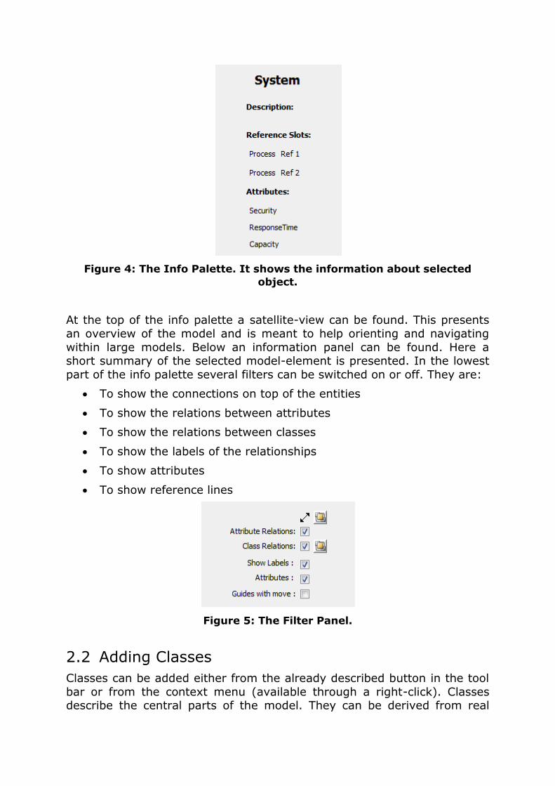
Figure 4: The Info Palette. It shows the information about selected

object.

At the top of the info palette a satellite-view can be found. This presents

an overview of the model and is meant to help orienting and navigating

within large models. Below an information panel can be found. Here a short summary of the selected model-element is presented. In the lowest

part of the info palette several filters can be switched on or off. They are:

To show the connections on top of the entities

To show the relations between attributes

To show the relations between classes

To show the labels of the relationships

To show attributes

To show reference lines

Figure 5: The Filter Panel.

2.2 Adding Classes

Classes can be added either from the already described button in the tool

bar or from the context menu (available through a right-click). Classes describe the central parts of the model. They can be derived from real

objects, such as “person” or “system”. Also a more abstract level of

entities is possible, such as “function” or “process”, which have no

physical real world counterpart. They are depicted like classes in a class diagram as a rectangle with the name of the class at the top of the box

and a line separating it from the rest of the box.

Classes can inherit properties from already existing classes, which can be

selected from their context menu, therefore the option “Set Superclass” needs to be used.

Classes can be attributed (see description below). It is also possible to “bring to front” them, so that they get visible even in complex models. A

description might be add from the context menu too.

Figure 6: Context menu for a Class. Set Super Class option will lead to

following dialog.

Figure 7: Set Super Class Dialog.

2.3 Adding Slots

Classes can be related to each other via slots. This is done by holding the

ctrl-key and drawing a relation from one Class to another one. Afterwards

those slots can be configured from their context menu (available through a right-click).

Figure 8: Context menu for Slot Reference.

Three options are possible at first the properties of the slots can be set,

second the routing can be adjusted and third they can be deleted. The properties that can be adjusted are multiplicities, role-names and the

name of the slots in general. If the routing is activated than a double-click on a slot allows to either set or remove a control point (which is a fixed

point that is part of a slot).

Figure 9: Slot Reference Properties.

It is also possible to add a slot from a certain Class to the same again. This is done via the “Self-References” menu of the Class’ context menu.

Figure 10: Self Reference menu.

Either undirected or directed self-references can be used.

Figure 11: Undirected Self Reference.

The difference is that undirected self-references can be used to relate

attributes of an object of Class A to a second one and the other way around, whereas directed one only allow relations from one object to

another one.

Slots determine which and how many relations are possible in the

instantiations (see below).

Figure 12: Directed Self Reference and Properties of Self Reference.

Figure 13: Directed Self Reference will be shown by directed self

reference icon on top of class.

2.4 Adding Attributes

Attributes are used to describe Classes. They can be added from the context menu of a certain class. Several types of Attributes are supported,

which are explained in detail below.

Figure 14: Adding New Attribute.

A description can be added to all Attributes, this function is executed from the attribute’s context menu.

2.4.1 Adding Discrete Attributes

Discrete Attributes allow the description of classes in terms of states. On default the used states are high, medium, and low. But this can be

changed through the “Set Attribute Properties” function. It is also possible to use 1,2,3,4, and 5 or true and false. Additionally even customized

states are possible. This can be figured in the upper part of the Set CPM dialog.

Figure 15: Setting CPM for Discrete Attribute.

In case of customized states the plus-button allows the adding of

additional states. The probabilities that the considered variable is in a certain state (on a scale from 0 to 1) based on its potential parents can be

set in this dialog.

2.4.2 Adding Continuous Attributes

Continuous Attributes allow the description of classes in terms of mathematical equations (which even can be probability distribution

functions). The “Set Attribute Properties” function opens a dialog that allows these equations to be set.

Figure 16: Properties Dialog for Continuous Attributes.

The supported functions and operations are shown in the Functions and

Operations list (on the right) and can be added to the equation via either drag & drop or by hand. The attributes of nodes that can be used to create

a certain equation are shown in the list Available Nodes. If the mouse-pointer is over a node in that list, the reference slot, that a certain

attribute is taken from, is shown. The attributes can be inserted into an

equation via drag & drop too. The largest part of this dialog is the box that allows the creation of equations, that can be built based upon the already

described concepts. If ctrl and space are pressed, auto-completion is

performed or the user is presented with possible candidates for

completion.

Finally in the lower part of the dialog the bounds can be set, which are

used in case that functions are used.

2.5 Adding Attribute Relationships

As already described above, Attributes can be affected by other attributes.

This has to happen with consideration of the types of the attributes (i.e.

only continuous Attributes can be related to continuous attributes and only discrete attributes are allowed to get linked to discrete ones). Attribute

Relations need to be based on Slots (where an internal Attribute relationship is an exception (see below)). Therefore at first slots need to

be present, before Attributes can be related. This can also be done iterative.

When slots are present two attributes can be related by holding the ctrl key and drawing a connection from the first to the second one. Once this

is done a dialog is shown that allows selecting the slots that the attribute relationship is based on.

Figure 17: Path Determination Dialog for Attributes Relation.

Sequentially from source to target slots can be selected that are used as

basis to this Attribute relationship. When the target is reached green icons symbolize that the relation is valid. Yellow arrows allow going one step

back, when a correction of the path is needed.

Attributes need to be related in order to serve as input to each other. This means that in case that discrete Attributes are used, the states of the

Attributes only appear, when the Attributes have been related previously. For continuous variables it means that before Attributes can be used in

equations they need to be related.

2.5.1 Adding of internal Attribute Relationships

Attributes of the same class might also be related without the usage of

slots, so that they are related on each instantiation of that Class automatically. The relation is created as all others are. In the dialog that

is presented the box “Internal Reference” needs to be checked afterwards.

2.5.2 Setting of aggregation functions

Aggregation functions describe how several instances of the same Attribute are combined during the calculation. The usage of aggregation

functions is needed as during the theory-modeling the amount of linked instances is unclear (i.e. aggregation functions make the theory prepared

to handle dynamic aspects of the instantiations).

As aggregation functions are used to handle dynamic aspects they are

only used when several nodes need to be aggregated. This means that in case of only one parent is allowed (through multiplicities) no aggregation

is necessary. Whereas if the amount of parents is unclear (* multiplicity) they are utilized. To overcome the fact that there also might be zero

parents modeled a “Default CPT” can be set (the option is available in an Attribute Relationship’s context menu), which serves as alternative input

in case of nothing else being available.

Figure 18: Default CPT Dialog for Attributes Relation.

2.5.2.1 Setting of discrete aggregation functions

Discrete attributes can be aggregated through Max, Min or Average CPTs.

The function of them is described in MEKs and PJs book. The states of the default CPT match the states of the attribute they are supposed to

replace.

Figure 19: Aggregation Functions for Attributes Relation.

2.5.2.2 Setting of continuous aggregation functions

Continuous attributes can be aggregated through summation, product or

calculation of average.

Figure 20: Aggregation function for continuous attributes.

A default equation can be set as well. The dialog is similar to the one for

setting Attribute properties; the only difference is that no variables in terms of other Attributes can be used.

Figure 21: Default Equation for continuous Attribute.

3 Modeling in EA2T Concrete Modeler

The theory specified in the Abstract modeler can be applied in the

concrete part of the tool.

3.1 Starting EA2T

The EA2T concrete modeler is written in Java to enable platform

independence and thus requires Java JRE® to run (if missing, it can be

downloaded at http://www.java.com). For windows users the program is

started by running from the command line using the command

java –jar ConcreteModellerIPrm

alternatively a double-click on ConcreteModellerIPrm.jar starts the tool

too. .

3.1.1 Getting familiar with the user interface

When starting the concrete modeler the following dialog is displayed:

Figure 1: Start Up Dialog.

Here the user might load a previously done model and continue his work

on that or he can start with an empty model. As an empty model needs to

be based upon a predefined theory this needs to be loaded in order to

start otherwise.

Afterwards the following window is displayed:

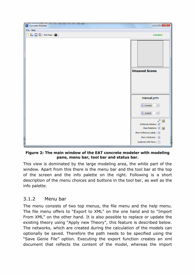
Figure 2: The main window of the EAT concrete modeler with modeling

pane, menu bar, tool bar and status bar.

This view is dominated by the large modeling area, the white part of the

window. Apart from this there is the menu bar and the tool bar at the top

of the screen and the info palette on the right. Following is a short

description of the menu choices and buttons in the tool bar, as well as the

info palette.

3.1.2 Menu bar

The menu consists of two top menus, the file menu and the help menu.

The file menu offers to “Export to XML” on the one hand and to “Import

From XML” on the other hand. It is also possible to replace or update the

existing theory using “Apply new Theory”, this feature is described below.

The networks, which are created during the calculation of the models can

optionally be saved. Therefore the path needs to be specified using the

“Save Genie File” option. Executing the export function creates an xml

document that reflects the content of the model, whereas the import

allows reading a model from xml file, which has been created earlier.

Additionally the program can be closed from the file menu.

Figure 3: Menu of Concrete Modeller

3.1.3 Tool bar

The toolbar, as displayed below, allows for easy access to the most

common functions of the tool

Figure 4: The toolbar of the EAT concrete modeller, containing the most

common commands.

Starting from the left there, at first the possibility to clear the scene and thereby to start with a new model can be found. The second function

allows opening of an existing model. This is followed by both save and saves as … functionalities. A button to add classes is offered next, which

even allows the instantiation of several classes at a time.

Figure 5: Multi Instantiation Dialog

Screenshots of the model can be made as well. Finally the “Calculate”

button allows evaluating a model.

3.1.4 Info palette

Information on the current model is presented in this information area.

Figure 6: Satellite-View

At the top of the info palette a satellite-view can be found. This presents an overview of the model and is meant to help orienting and navigating

within large models. Below information panel can be found. Here a short summary of the selected model-element is presented.

Figure 7: Info Palette showing information of Server (System)

The third panel allows to instantiate the classes contained in the used

theory. The amounts of instantiations at a time can be set via spinners.

Figure 8: Instantiation Panel

In the lowest part of the info palette several filters can be switched on or off. They are:

To show the connections on top of the entities

To show the relations between attributes

To show the relations between classes

To show the labels of the relationships

To show attributes

To show reference lines

Figure 9: Filter Panel

3.2 Instantiating Classes

Classes are instantiated from the tool bar as described above or by

selecting the amount of Objects in the info palette.

Instantiating a Class means that the created Object has attributes

associated with that type in the abstract model. For instance, the class

“system” might contain attributes such as information security or

performance whereas for the class “process” attributes such as efficiency

or cycle time could be appropriate. (The exact attributes of the classes as

well as what classes that are available is specified by the abstract model

(the theory) – developed in the EA2T Abstract Modeler.)

3.3 Instantiating relationships

Relationships are created between two classes and specify which relation

those classes have. Which relationships are valid is defined in the

underlying abstract model.

To create a relationship, press and hold the Ctrl key while dragging

between the classes. The order of source and target is not

In this dialog it is possible to choose which relationship to create, using

the drop down list, since there might be more than one option that is valid

according to the abstract model.

Figure 10: Relation Selection Panel

3.4 Adding evidence

Creating instances of classes and relationships builds up the skeleton of

the model. This provides basic knowledge for performing the assessment,

based upon prior knowledge about the various attributes (i.e. properties)

of the model. In order for the assessment to be specific for the case at

hand, this skeleton must be augmented with information about the actual

states of the attributes in the model.

In most cases, it is very difficult to have direct knowledge about complex

attributes such as the information security of an enterprise (otherwise this

tool would serve little purpose). However, more low-level attributes such

as minimum password length or number of open ports in the firewall can

usually be found. While this information is generally not hard to find, it is

potentially very resource demanding to actually gather it all. The concept

of evidence handles this. Evidence is knowledge about the actual states of

attributes that is not certain, but has a level of credibility that can be

taken into account when performing the analysis. The EA2T concrete

modeler allows the user to provide evidence(s) regarding the states of

every attribute, including the more complex ones, in case such knowledge

is available.

The way evidence is set depends on the kind of the Attribute that is

considered.

3.4.1 Adding evidence for discrete Attributes

Evidence regarding the state of a discrete attribute is given by right

clicking the attribute and selecting “Evidence”. Figure 11 illustrates the

display that appears.

Figure 11: The evidence dialog where John in an interview claims that

the attribute is in state "Medium" with a 95% probability.

To add evidence on the attribute, enter a name on the evidence, select

which of the attributes states to add evidence about, fill in the credibility

matrix and press “add evidence” in the lower left region of the dialog. In

the example in Figure the evidence “John” (corresponding to the result of

an interview with a John) claims that the attribute, in this case Cyber

security policy fulfillment (from NERC-CIP 003) is in state medium. The

credibility is 95% (a more detailed discussion about credibility follows in

the next section).

It is possible to add multiple evidence on an attribute, including conflicting

evidence. This reflects the possibility of disagreement, uncertainty and

even deliberate deception. All evidence added to an attribute will be

shown in the list at the top of the dialog. It is also possible to remove

evidence by selecting it in the list and pressing “delete evidence”.

Attribute might be updated in case that e.g. wrong data has been saved.

This is done by at first clicking on existing evidence. Afterwards the

evidence is displayed. It might be modified afterwards and finally stored

through a click on the “Update Evidence” button.

If its 100% assure that an Attribute is in a certain state this can also be

expressed by fixing that Attribute to always assume that state. The

context menu of that Attribute offers therefore the function “Set State”.

Out of all the possible states that the Attribute might be in, the right one

can be chosen.

3.4.1.1 Credibility Matrix

The credibility matrix makes it possible to express the credibility of a

source of evidence. The matrix represents the probability that the

attribute is in each of its states, given the evidence. More formally the

matrix specifies where A is the attribute and E is the evidence. In

the current version of the tool, this matrix is predefined to the one shown

in Figure which should be interpreted as follows: Given an evidence that

the attribute is in state high there is a 95% probability that the attribute

actually is in the state high and a 2,5% probability that the attribute is in

state medium or low respectively. Similarly, given evidences on states

medium or low there is a 95% probability that the attribute is in the same

state as the evidence and a 2,5% probability that it is in any of the other

states. Future versions of the tool will allow the modeler to define this

matrix according to the type of evidence used. (Some information sources

are simply more credible than others!)

3.4.2 Adding evidence for continuous Attributes

Evidence regarding the state of a concrete attribute is given by right

clicking the attribute and selecting “Evidence”. Figure 12 illustrates the

display that appears.

Figure 12: The evidence dialog For Continuous Attribute.

This attribute can be described in terms of either a fixed.

3.5 Calculating the model

Once the model is complete in terms of objects, relationships, and

evidence on the attributes, it is possible to perform the actual assessment.

Since each concrete model has an underlying abstract model that defines

the theory, the user only have to request that the analysis is to take

place. The theory is then applied to the model using and all the attributes

are evaluated..

The Model is calculated by pressing the “calculate” button in the tool bar.

To display the result of the assessment, right click on the attribute of

interest the “Show values” option. The results of the assessment are

displayed according to the type of attribute that is considered. Discrete

attributes are presented as probability distributions. In the example given

in Figure10 below, it is possible to see that the degree of preparedness for

occurrence of incidents is assessed to being high with a 65 % probability,

medium with a 25% probability and low with 10 % probability.

Figure 13: The result of an assessment, showing a probability

distribution for the attribute Degree of preparedness for

occurrence of incidents.

Continuous variables are either presented as single value or as probability

distribution, depending on the result. The distributions are presented in

terms of:

Mean value

Variance

Skewness

Kurtosis

Samples

Histogram with individual amount of bins

Figure 14: Single Value.

Figure 15: Probability Distribution.

3.6 Replacement of used theory

As mentioned previously, the tool supports the replacement and update of

the used theory. The tool tries to match and perform updates as far as

possible completely autonomously. In case of ambiguities the tool

questions the user to solve them.

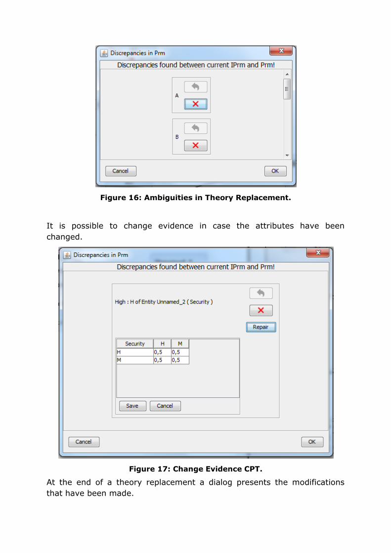
Figure 16: Ambiguities in Theory Replacement.

It is possible to change evidence in case the attributes have been

changed.

Figure 17: Change Evidence CPT.

At the end of a theory replacement a dialog presents the modifications

that have been made.

4 Quick reference

Abstract modeler. The abstract modeler is the part of the EA2T where

the underlying theory for enterprise architecture assessments is specified.

Here, the concepts and relationships relevant for different kinds of

analysis is defined, thus enabling the users of the concrete modeler to

perform advanced assessments in an automatic, easy fashion.

Bayesian network. A Bayesian network is a probabilistic graphical model

that represents a set of variables and their probabilistic dependencies.

Bayesian networks combine a rigorous mathematical handling of

uncertainty with a graphical and intuitive depiction of causal relationships

between different phenomena. Bayesian calculations are at the heart of

enterprise architecture analysis using the EA2T.

Concrete modeler. The concrete modeler is used to model concrete

instances of system scenarios. The concrete modeler uses the theoretical

framework developed in the abstract modeler to direct and enable

complicated enterprise architecture analyses, without a need for the user

to be a theoretical expert. The concrete modeler is mainly intended to be

used by enterprise architects in the industry.

Class. A class is a category that entities can belong to. When an entity in

a concrete model belongs to a class, it means that it has some attributes

associated with that class as defined in the abstract model. For instance,

the class “system” might contain attributes such as “information security”

or “performance” whereas for the class “process” might have attributes

such as “efficiency” or “cycle time”.

Credibility. Different data have different credibility, depending on

whether the source is reliable, whether it is recently collected etc. When

conducting enterprise architecture analyses, it is of great importance that

models and decisions are not based on flawed or biased data. By requiring

the user to specify the credibility of the data used, the EA2T tool manages

this aspect of data collection.

Enterprise architecture. The discipline of advocates the use of models

to support decision-making on enterprise-wide information system issues.

By analyzing the relevant data in a structured, and preferably

quantitative, way, better management decisions can be made.

Entity. An entity is a modeling concept, usually referring to something

that is an object in the real world. Enterprise, CRM system, computer, and

project team are all examples of possible entities. Entities have attributes

and belong to classes.

Evidence. Evidence is the data about real world circumstances, collected

for the purpose of enterprise architecture analysis. Such evidence is never

certain, but rather has a level of credibility that can be taken into account

when performing the analysis. The EA2T concrete modeler allows the user

to provide evidence(s) regarding the states of every attribute, including

the more complex ones, should such knowledge be available.

Model. A model is a simplified representation of the real world,

specifically designed to capture the aspects relevant for a certain purpose,

and leave other aspects out. Enterprise architecture models try to

incorporate those features relevant to decision making on enterprise-wide

information system issues. The EA2T tool distinguishes two types of

models: the abstract model that speak of general relationships between

entities such as availability and maintenance organizations, and concrete

models that speak of particular companies and situations, such as the

availability of system X on company Y. The idea is that the abstract

models are provided by researchers as support for the industry that deals

primarily with concrete models.

Object. See Entity

Relationship. Relationships describe how different classes relate to each

other. Observable regularities in the real world are modeled as

relationships, such as when the “reliability of components decreases, the

maintenance costs increase”. Relationships based on research are created

in the abstract modeler, where they serve as templates for analyses in the

concrete modeler.