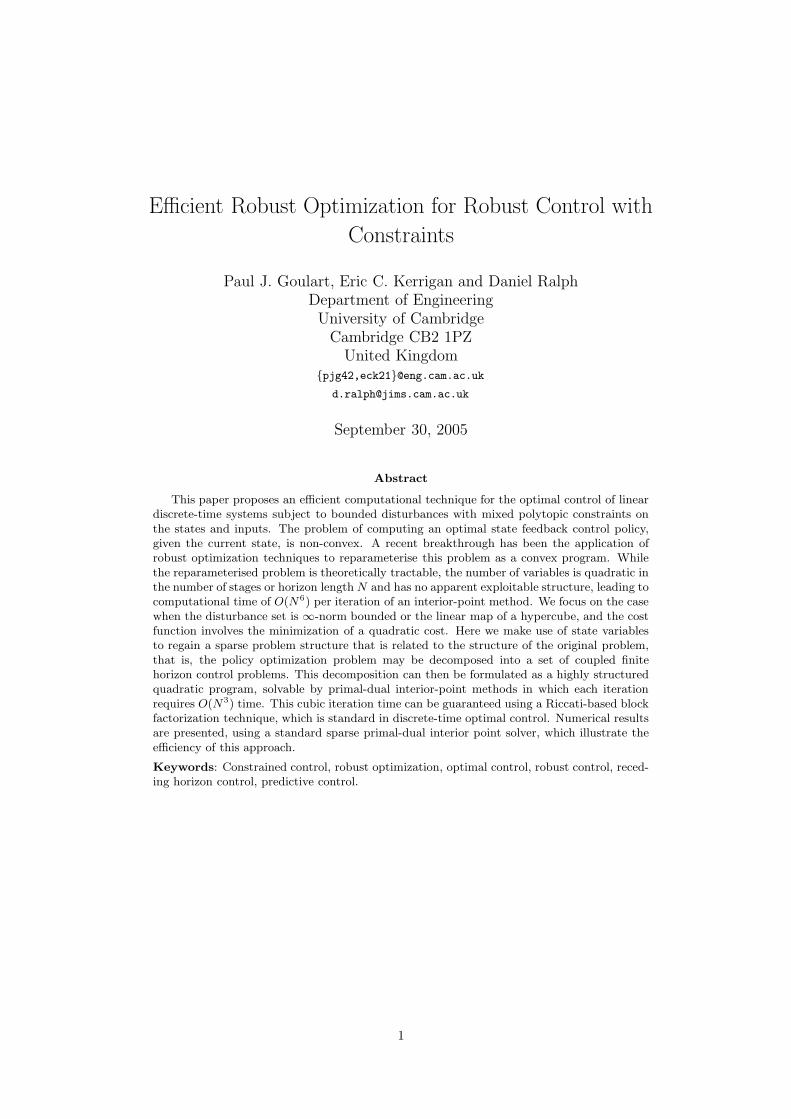
Efficient Robust Optimization for Robust Control with

Constraints

Paul J. Goulart, Eric C. Kerrigan and Daniel Ralph

Department of Engineering

University of Cambridge

Cambridge CB2 1PZ

United Kingdom

{pjg42,eck21}@eng.cam.ac.uk

d.ralph@jims.cam.ac.uk

September 30, 2005

Abstract

This paper proposes an efficient computational technique for the optimal control of lineardiscrete-time systems subject to bounded disturbances with mixed polytopic constraints onthe states and inputs. The problem of computing an optimal state feedback control policy,given the current state, is non-convex. A recent breakthrough has been the application ofrobust optimization techniques to reparameterise this problem as a convex program. Whilethe reparameterised problem is theoretically tractable, the number of variables is quadratic inthe number of stages or horizon length N and has no apparent exploitable structure, leading tocomputational time of O(N6) per iteration of an interior-point method. We focus on the casewhen the disturbance set is ∞-norm bounded or the linear map of a hypercube, and the costfunction involves the minimization of a quadratic cost. Here we make use of state variablesto regain a sparse problem structure that is related to the structure of the original problem,that is, the policy optimization problem may be decomposed into a set of coupled finitehorizon control problems. This decomposition can then be formulated as a highly structuredquadratic program, solvable by primal-dual interior-point methods in which each iterationrequires O(N3) time. This cubic iteration time can be guaranteed using a Riccati-based blockfactorization technique, which is standard in discrete-time optimal control. Numerical resultsare presented, using a standard sparse primal-dual interior point solver, which illustrate theefficiency of this approach.

Keywords: Constrained control, robust optimization, optimal control, robust control, reced-ing horizon control, predictive control.

1

1 Introduction

Robust and predictive control

This paper is concerned with the efficient computation of optimal control policies for constraineddiscrete-time linear systems subject to bounded disturbances on the state. In particular, weconsider the problem of finding, over a finite horizon of length N , a feedback policy

π := {µ0(·), . . . , µN−1(·)} (1)

for a discrete-time linear dynamical system of the form

xi+1 = Axi + Bui + wi (2)

ui = µi(x0, . . . , xi) (3)

which guarantees satisfaction of a set of mixed constraints on the states and inputs at each time,for all possible realizations of the disturbances wi, while minimizing a given cost function.

The states xi and inputs ui are constrained to lie in a compact and convex set Z , i.e.

(xi, ui) ∈ Z , ∀i ∈ {0, 1, . . . , N − 1} (4)

with an additional terminal constraint xN ∈ Xf . We assume nothing about the disturbances butthat they lie in a given compact set W .

The above, rather abstract problem is motivated by the fact that for many real-life control ap-plications, optimal operation nearly always occurs on or close to some constraints [36]. Theseconstraints typically arise, for example, due to actuator limitations, safe regions of operation, orperformance specifications. For safety-critical applications, in particular, it is crucial that someor all of these constraints are met, despite the presence of unknown disturbances.

Because of its importance, the above problem and derivations of it have been studied for sometime now, with a large body of literature that falls under the broad banner of “robust control”(see [5, 49] for some seminal work on the subject). The field of linear robust control, which ismainly motivated by frequency-domain performance criteria [52] and does not explicitly considertime-domain constraints as in the above problem formulation, is considered to be mature and anumber of excellent references are available on the subject [16, 23, 53]. In contrast, there are fewtractable, non-conservative solutions to the above, constrained problem, even if all the constraintsets are considered to be polytopes or ellipsoids; see, for example, the literature on set invariancetheory [7] or `1 optimal control [12, 17, 44, 46].

A control design method that is particularly suitable for the synthesis of controllers for systemswith constraints, is predictive control [10, 36]. Predictive control is a family of optimal controltechniques where, at each time instant, a finite-horizon constrained optimal control problem issolved using tools from mathematical programming. The solution to this optimization problemis usually implemented in a receding horizon fashion, i.e. at each time instant, a measurement ofthe system is obtained, the associated optimization problem is solved and only the first controlinput in the optimal policy is implemented. Because of this ability to solve a sequence of compli-cated, constrained optimal control problems in real-time, predictive control is synonymous with“advanced control” in the chemical process industries [40].

The theory on predictive control without disturbances is relatively mature and most of the fun-damental problems are well-understood. However, despite recent advances, there are many openquestions remaining in the area of robust predictive control [3, 37, 38]. In particular, efficient op-timization methods have to be developed for solving the above problem before robust predictivecontrol methods can be applied to unstable or safety-critical applications in areas such as aerospaceand automotive applications [45].

2

Robust control models

The core difficulty with the problem (1)–(4) is that optimizing the feedback policy π over arbitrarynonlinear functions is extremely difficult, in general. Proposals which take this approach, suchas [43], are intractable for all but the smallest problems, since they generally require enumeration ofall possible disturbance realizations generated from the set W . Conversely, optimization over open-loop control sequences, while tractable, is considered unacceptable since problems of infeasibilityor instability may easily arise [38].

An obvious sub-optimal proposal is to parameterize the control policy π in terms of affine functionsof the sequence of states, i.e. to parameterize the control sequence as

ui =

i∑

j=0

Li,jxj + gi (5)

where the matrices Li,j and vectors gi are decision variables. However, the set of constraintadmissible policies of this form is easily shown to be non-convex in general. As a result, most pro-posals that take this approach [2,11,29,32,39] fix a stabilising feedback gain K, then parameterizethe control sequence as ui = Kxi + gi and optimize the design parameters gi. This approach,though tractable, is problematic, as it is unclear how one should select the gain K to minimizeconservativeness.

A recent breakthrough [22] showed that the problem of optimizing over state feedback policies ofthe form (5) is equivalent to a convex optimization problem using disturbance feedback policiesof the form

ui =

i−1∑

j=0

Mi,jwj + vi. (6)

Robust optimization modelling techniques [4,24] are used to eliminate the unknown disturbances wj

and formulate the admissable set of control policies with O(N 2mn) variables, where N is the hori-zon length as above, and m and n are the respective dimensions of the controls ui and states xi ateach stage. This implies that, given a suitable objective function, an optimal affine state feedbackpolicy policy (5) can be found in time that is polynomially bounded in the size of the problemdata.

Efficient computational in robust optimal control

In the present paper we demonstrate that an optimal policy of the form (6), equivalently (5),can be efficiently calculated in practise, given suitable polytopic assumptions on the constraintsets W , Z and Xf . This result is critical for practical applications, since one would generallyimplement a controller in a receding horizon fashion by calculating, on-line and at each timeinstant, an admissible control policy (5), given the current state x. Such a control strategy hasbeen shown to allow for the synthesis of stabilizing, nonlinear time-invariant control laws thatguarantee satisfaction of the constraints Z for all time, for all possible disturbance sequencesgenerated from W [22].

While convexity of the robust optimal problem arising out of (6) is key, the resulting optimizationproblem is a dense convex quadratic program with O(N 2) variables (see Section 4, cf. [22]),assuming N dominates the dimension of controls m and states n at each stage. Hence eachiteration of an interior-point method will require solving a dense linear system and thus requireO(N6) time. This situation is common, for example, in the rapidly growing number of aerospaceand automotive applications of predictive control [36, Sec. 3.3] [40]. We show that when thedisturbance set is ∞-norm bounded or the linear map of a hypercube, the special structure of therobust optimal control problem can be exploited to devise a sparse formulation of the problem,thereby realizing a substantial reduction in computational effort to O(N 3) work per interior-pointiteration.

3

We demonstrate that the cubic-time performance of interior-point algorithms at each step can beguaranteed when using a factorization technique based on Riccati recursion and block elimination.Numerical results are presented that demonstrate that the technique is computationally feasiblefor systems of appreciable complexity using the standard sparse linear system solver MA27 [26]within the primal-dual interior-point solver OOQP [19]. We compare this primal-dual interior-point approach to the sparse active-set method PATH [14] on both the dense and sparse problemformulations. Our results suggest that the interior-point method applied to the sparse formulationis the most practical method for solving robust optimal control problems, at least in the “coldstart” situation when optimal active set information is unavailable.

A final remark is that the sparse formulation of robust optimal control results from a decompositiontechnique that can be used to separate the problem into a set of coupled finite horizon controlproblems. This reduction of effort is the analogue, for robust control, to the situation in classicalunconstrained optimal control in which Linear Quadratic Regulator (LQR) problems can be solvedin O(N) time, using a Riccati [1, Sec. 2.4] or Differential Dynamic Programming [27] technique inwhich the state feedback equation x+ = Ax + Bu is explicit in every stage, compared to O(N 3)time for the more compact formulation in which states are eliminated from the system. Moredirect motivation for our work comes from [6,13, 41, 50], which describe efficient implementationsof optimization methods for solving optimal control problems with state and control constraints,though without disturbances.

Contents

The paper is organized as follows: Sections 2 and 3 introduce the optimal control problem consid-ered throughout the paper. Sections 4 and 5 describe the equivalent affine disturbance feedbackpolicy employed to solve the optimal control problem, as well as an equivalent formulation whichcan be decomposed into a highly structured, singly-bordered block-diagonal quadratic programthrough reintroduction of appropriate state variables. Section 6 demonstrates that, when using aprimal-dual interior-point solution technique, the decomposed quadratic program can always besolved in time cubic in the horizon length at each interior-point iteration. Section 7 demonstratesthrough numerical examples that the proposed decomposition can be solved much more efficientlythan the equivalent original formulation, and the paper concludes in Section 8 with suggestionsfor further research.

2 Definitions and Standing Assumptions

Consider the following discrete-time linear time-invariant system:

x+ = Ax + Bu + w, (7)

where x ∈ Rn is the system state at the current time instant, x+ is the state at the next time

instant, u ∈ Rm is the control input and w ∈ R

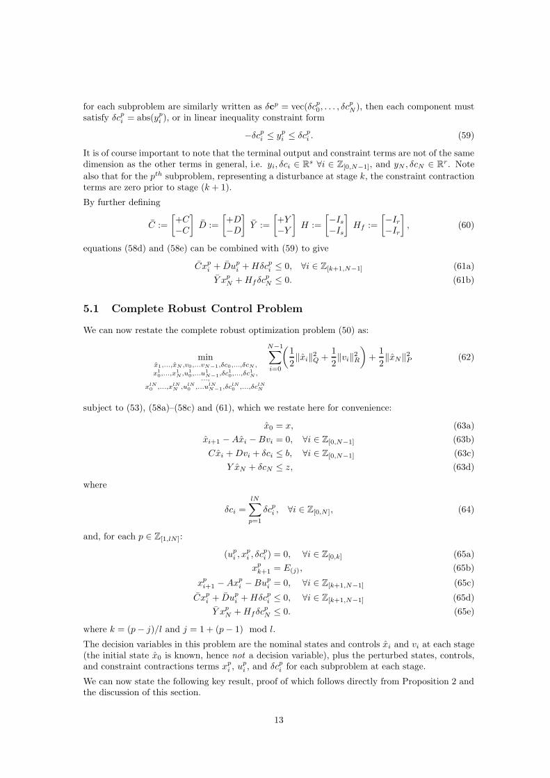
n is the disturbance. It is assumed that (A, B) isstabilizable and that at each sample instant a measurement of the state is available. It is furtherassumed that the current and future values of the disturbance are unknown and may changeunpredictably from one time instant to the next, but are contained in a convex and compact(closed and bounded) set W , which contains the origin. Initially, we make no further assumptionson the set W .

The system is subject to mixed constraints on the state and input:

Z := {(x, u) ∈ Rn × R

m | Cx + Du ≤ b} , (8)

where the matrices C ∈ Rs×n, D ∈ R

s×m and the vector b ∈ Rs; s is the number of affine inequality

constraints that define Z . It is assumed that Z is bounded and contains the origin in its interior.

4

A design goal is to guarantee that the state and input of the closed-loop system remain in Z forall time and for all allowable disturbance sequences.

In addition to Z , a target/terminal constraint set Xf is given by

Xf := {x ∈ Rn | Y x ≤ z } , (9)

where the matrix Y ∈ Rr×n and the vector z ∈ R

r; r is the number of affine inequality constraintsthat define Xf . It is assumed that Xf is bounded and contains the origin in its interior. Theset Xf can, for example, be used as a target set in time-optimal control or, if defined to berobust positively invariant, to design a receding horizon controller with guaranteed invariance andstability properties [22].

Before proceeding, we define some additional notation. In the sequel, predictions of the system’sevolution over a finite control/planning horizon will be used to define a number of suitable controlpolicies. Let the length N of this planning horizon be a positive integer and define stacked versionsof the predicted input, state and disturbance vectors u ∈ R

mN , x ∈ Rn(N+1) and w ∈ R

nN ,respectively, as

x := vec(x0, . . . , xN−1, xN ),

u := vec(u0, . . . , uN−1),

w := vec(w0, . . . , wN−1),

where x0 = x denotes the current measured value of the state and xi+1 := Axi + Bui + wi,i = 0, . . . , N − 1 denotes the prediction of the state after i time instants into the future. Finally,let the set W := W N := W × · · · × W , so that w ∈ W .

3 An Affine State Feedback Parameterization

One natural approach to controlling the system in (7), while ensuring the satisfaction of theconstraints (8)–(9), is to search over the set of time-varying affine state feedback control policies.We thus consider policies of the form:

ui =

i∑

j=0

Li,jxj + gi, ∀i ∈ Z[0,N−1], (11)

where each Li,j ∈ Rm×n and gi ∈ R

m. For notational convenience, we also define the block lowertriangular matrix L ∈ R

mN×n(N+1) and stacked vector g ∈ RmN as

L :=

2

6

4

L0,0 0 · · · 0...

. . .. . .

...LN−1,0 · · · LN−1,N−1 0

3

7

5, g :=

2

6

4

g0

...gN−1,

3

7

5, (12)

so that the control input sequence can be written as u = Lx + g. For a given initial state x(since the system is time-invariant, the current time can always be taken as zero), we say thatthe pair (L,g) is admissible if the control policy (11) guarantees that for all allowable disturbancesequences of length N , the constraints (8) are satisfied over the horizon i = 0, . . . , N − 1 and thatthe state is in the target set (9) at the end of the horizon. More precisely, the set of admissible(L,g) is defined as

ΠsfN (x) :=

(L,g)

∣

∣

∣

∣

∣

∣

∣

∣

∣

∣

(L,g) satisfies (12), x = x0

xi+1 = Axi + Bui + wi

ui =∑i

j=0 Li,jxj + gi

(xi, ui) ∈ Z , xN ∈ Xf

∀i ∈ Z[0,N−1], ∀w ∈ W

(13)

5

and the set of initial states x for which an admissible control policy of the form (11) exists isdefined as

XsfN :=

{

x ∈ Rn∣

∣

∣Πsf

N (x) 6= ∅}

. (14)

It is critical to note that, in general, it is not possible to select a single pair (L,g) such that

(L,g) ∈ ΠsfN (x) for all x ∈ Xsf

N . Indeed, it is possible that for some pair (x, x) ∈ XsfN × Xsf

N ,

ΠsfN (x)

⋂

ΠsfN (x) = ∅.

For problems of non-trivial size, it is therefore necessary to calculate an admissible pair (L,g)on-line, given a measurement of the current state x, rather than fixing (L,g) off-line. Once anadmissible control policy is computed for the current state, it can be implemented either in aclassical time-varying, time-optimal or receding-horizon fashion.

In particular, we define an optimal policy pair (L∗(x),g∗(x)) ∈ ΠsfN (x) to be one which minimizes

the value of a cost function that is quadratic in the disturbance-free state and input sequence. Wethus define:

VN (x,L,g,w) :=

N−1∑

i=0

1

2(‖xi‖

2Q+‖ui‖

2R)+

1

2‖xN‖2

P (15)

where x0 = x, xi+1 = Axi +Bui +wi and ui =∑i

j=0 Li,j xj + gi for i = 0, . . . , N − 1; the matricesQ and P are positive semidefinite, and R is positive definite. We define an optimal policy pair as

(L∗(x),g∗(x)) := argmin(L,g)∈Πsf

N (x)

VN (x,L,g,0). (16)

Before proceeding, we also define the value function V ∗N : Xsf

N → R≥0 to be

V ∗N (x) := min

(L,g)∈Πsf

N(x)

VN (x,L,g, 0). (17)

For the receding-horizon control case, a time-invariant control law µN : XsfN → R

m can beimplemented by using the first part of this optimal control policy at each time instant, i.e.

µN (x) := L∗0,0(x)x + g∗0(x). (18)

We emphasize that, due to the dependence of (13) on the current state x, the control law µN (·)will, in general, be a nonlinear function with respect to the current state, even though it may havebeen defined in terms of the class of affine state feedback policies (11).

Remark 1. Note that the state feedback policy (11) includes the well-known class of “pre-stabilizing”control policies [11,29,32,39], in which the control policy takes the form ui = Kxi + ci, where Kis computed off-line and only ci is computed on-line.

The control law µN (·) has many attractive geometric and system-theoretic properties. In partic-

ular, implementation of the control law µN (·) renders the set XsfN robust positively invariant, i.e.

if x ∈ XsfN , then it can be shown that Ax + BµN (x) + w ∈ Xsf

N for all w ∈ W , subject to certaintechnical conditions on the terminal set Xf . Furthermore, the closed-loop system is guaranteed tobe input-to-state (ISS) stable when W is a polytope, under suitable assumptions on Q, P , R, andXf . The reader is referred to [22] for a proof of these results and a review of other system-theoreticproperties of this parameterization.

Unfortunately, such a control policy is seemingly very difficult to compute, since the set ΠsfN (x)

and cost function VN (x, ·, ·, 0) are non-convex; however, it is possible to convert this non-convexoptimization problem to an equivalent convex problem through an appropriate reparameterization.This parameterization is introduced in the following section.

6

4 Affine Disturbance Feedback Control Policies

An alternative to (11) is to parameterize the control policy as an affine function of the sequenceof past disturbances, so that

ui =

i−1∑

j=0

Mi,jwj + vi, ∀i ∈ Z[0,N−1], (19)

where each Mi,j ∈ Rm×n and vi ∈ R

m. It should be noted that, since full state feedback isassumed, the past disturbance sequence is easily calculated as the difference between the predictedand actual states at each step, i.e.

wi = xi+1 − Axi − Bui, ∀i ∈ Z[0,N−1]. (20)

The above parameterization appears to have originally been suggested some time ago within thecontext of stochastic programs with recourse [18]. More recently, it has been revisited as as a meansfor finding solutions to a class of robust optimization problems, called affinely adjustable robustcounterpart (AARC) problems [4,24], and robust model predictive control problems [33,34,47,48].

Define the variable v ∈ RmN and the block lower triangular matrix M ∈ R

mN×nN such that

M :=

2

6

6

4

0 · · · · · · 0M1,0 0 · · · 0...

. . .. . .

...MN−1,0 · · · MN−1,N−2 0

3

7

7

5

, v :=

2

6

6

4

v0......vN−1

3

7

7

5

, (21)

so that the control input sequence can be written as u = Mw + v. Define the set of admissible(M,v), for which the constraints (8) and (9) are satisfied, as:

ΠdfN (x) :=

(M,v)

∣

∣

∣

∣

∣

∣

∣

∣

∣

∣

(M,v) satisfies (21), x = x0

xi+1 = Axi + Bui + wi

ui =∑i−1

j=0 Mi,jwj + vi

(xi, ui) ∈ Z , xN ∈ Xf

∀i ∈ Z[0,N−1], ∀w ∈ W

, (22)

and define the set of initial states x for which an admissible control policy of the form (19) existsas

XdfN := {x ∈ R

n | ΠdfN (x) 6= ∅}. (23)

As shown in [30], it is possible to eliminate the universal quantifier in (22) and construct matricesF ∈ R

(sN+r)×mN , G ∈ R(sN+r)×nN and T ∈ R

(sN+r)×n, and vector c ∈ RsN+r (defined in

Appendix A) such that the set of feasible pairs (M,v) can be written as:

ΠdfN (x) =

{

(M,v)

∣

∣

∣

∣

∣

(M,v) satisfies (21),

Fv + vec maxw∈W

(FM + G)w ≤ c + Tx

}

, (24)

where vecmaxw∈W(FM + G)w denotes row-wise maximization, i.e. if (FM + G)i denotes the ith

row of the matrix FM + G, then

vec maxw∈W

(FM + G)w := vec

(

maxw∈W

(FM + G)1w, . . . , maxw∈W

(FM + G)sN+rw

)

. (25)

Note that these maxima always exist when the set W is compact.

We are interested in this control policy parameterization primarily due to the following two prop-erties, proof of which may be found in [22]:

7

Theorem 1 (Convexity). For a given state x ∈ XdfN , the set of admissible affine disturbance

feedback parameters ΠdfN (x) is convex. Furthermore, the set of states Xdf

N , for which at least oneadmissible affine disturbance feedback parameter exists, is also convex.

Theorem 2 (Equivalence). The set of admissible states XdfN = Xsf

N . Additionally, given any

x ∈ XsfN , for any admissible (L,g) an admissible (M,v) can be constructed that yields the same

input and state sequence for all allowable disturbances, and vice-versa.

Together, these results enable efficient implementation of the control law u = µN (x) in (18) by re-placing the non-convex optimization problem (16) with an equivalent convex problem. If we definethe nominal states xi ∈ R

n to be the states when no disturbances occur, i.e. xi+1 = Axi + Bvi.and define x ∈ R

nN asx := vec(x, x1, . . . , xN ) = Ax + Bv. (26)

where A ∈ Rn(N+1)×n and B ∈ R

n(N+1)×mN are defined in Appendix A, then a quadratic costfunction similar to that in (15) can be written as

V dfN (x,v) :=

N−1∑

i=0

1

2(‖xi‖

2Q + ‖vi‖

2R) +

1

2‖xN‖2

P , (27)

or, in vectorized form, as

V dfN (x,v) =

1

2‖Ax + Bv‖2

Q +1

2‖v‖2

R (28)

where Q := [ I⊗QP

] and R := I ⊗ R. This cost can then be optimized over allowable policies in(24), forming a convex optimization problem in the variables M and v:

minM,v

V dfN (x,v) s.t. (M,v) ∈ Πdf

N (x) (29)

As a direct result of the equivalence of the two parameterizations, the minimum of V dfN (x, ·)

evaluated over the admissible policies ΠdfN (x) is equal to the minimum of VN (x, ·, ·, 0) in (16), i.e.

min(M,v)∈Πdf

N(x)V df

N (x,v) = min(L,g)∈Πsf

N(x)VN (x,L,g,0) (30)

The control law µN (·) in (18) can then be implemented using the first part of the optimal v∗(·)at each step, i.e.

µN (x) = v∗0(x) = L∗0,0(x)x + g∗0(x) (31)

where

(M∗(x),v∗(x)) := argmin(M,v)∈Πdf

N (x)

V dfN (x,v) (32)

v∗(x) =: vec(v∗0(x), . . . , v∗N−1(x)) (33)

which requires the minimization of a convex function over a convex set. The receding horizoncontrol law µN (·) in (18) is thus practically realizable. Note that since the cost function (27) isstrictly convex in v, both the minimizer v∗(x) and the resulting control law (31) are uniquelydefined for each x [42, Thm 2.6], and the value function V ∗

N (·) is convex and continuous on the

interior of XsfN [42, Thm. 2.35, Cor. 3.32].

Until this point, no constraints have been imposed on the disturbance set W other than therequirement that it be compact; Theorems 1 and 2 hold even for non-convex disturbance sets. Inthe remainder of this section, we consider the special cases where W is a polytopic or ∞-normbounded set.

8

4.1 Optimization Over Polytopic Disturbance Sets

We consider the special case where the constraint set describes a polytope (closed and boundedpolyhedron). In this case the disturbance set may be written as

W ={

w ∈ RnN | Sw ≤ h

}

(34)

where S ∈ Rt×n and h ∈ R

t (note that this includes cases where the disturbance set is timevarying). Note that both 1- and ∞-norm disturbance sets W can be characterized in this manner.

In this case, we can write the dual problem for each row of vec maxw∈W(FM + G)w, and solvethe convex control policy optimization problem (29) as a single quadratic program.

4.1.1 Introduction of Dual Variables to the Robust Problem

With a slight abuse of notation, we recall that for a general LP in the form

minz

cT z, s.t. Az = b, z ≥ 0 (35)

the same problem can be solved in dual form by solving the dual problem

maxw

bT w, s.t. AT w ≤ c (36)

where, for each feasible pair (z, w), it is always true that bT w ≤ cT z. Using this idea, if we definethe ith row of (FM + G) as (FM + G)i, then the dual of each row of (25) can be written as

maxw∈W

(FM + G)iw = minzi

hT zi, s.t. ST zi = (FM + G)Ti , zi ≥ 0, (37)

where the vectors zi ∈ Rt represents the dual variables associated with the ith row. By combining

these dual variables into a matrixZ :=

[

z1 . . . zN

]

(38)

the set ΠdfN (x) can be written in terms of purely linear constraints:

ΠdfN (x) =

(M,v)

∣

∣

∣

∣

∣

∣

∣

(M,v) satisfies (21), ∃Z s.t.

Fv + ZT h ≤ c + Tx

FM + G = ZT S, Z ≥ 0

, (39)

where all inequalities are element-wise.

Note that the convex optimization problem (29) now requires optimization over the polytopic set(39), leading to a quadratic programming problem in the variables M, Z and v.

Remark 2. When the disturbance set is polytopic, it can be shown that the value function V ∗N (·)

is piecewise quadratic on XN , and the resulting control law µN (·) is piecewise affine [22].

4.2 Optimization Over ∞-Norm Bounded Disturbance Sets

In the remainder of this paper, we consider the particular case where W is generated as the linearmap of a hypercube. Define

W = {w ∈ Rn | w = Ed, ‖d‖∞ ≤ 1}, (40)

where E ∈ Rn×l, so that the stacked generating disturbance sequence d ∈ R

lN is

d = vec(d0, . . . , dN−1), (41)

9

and define the matrix J := IN ⊗ E ∈ RNn×Nl, so that w = Jd. As shown in [30], an analytical

solution to the row-wise maximization in (24) is easily found. From the definition of the dualnorm [25], when the generating disturbance d is any p-norm bounded signal given as in (40), then

maxw∈W

aT w = ‖ET a‖q (42)

for any vector a ∈ Rn, where 1/p + 1/q = 1.

Straightforward application of (42) to the row wise-maximization in (24) (with q = 1) yields

ΠdfN (x) =

{

(M,v)(M,v) satisfies (21)

Fv + abs(FMJ + GJ)1 ≤ c + Tx

}

, (43)

where abs(FMJ + GJ)1 is a vector formed from the 1-norms of the rows of (FMJ + GJ). Thiscan be written as a set of purely affine constraints by introducing slack variables and rewriting as

ΠdfN (x) =

(M,v)(M,v) satisfies (21), ∃Λ s.t.

Fv + Λ1 ≤ c + Tx−Λ ≤ (FMJ + GJ) ≤ Λ

. (44)

As in the case for general polytopic disturbance sets, the cost function (27) can then be minimizedover allowable policies in (44) by forming a quadratic program in the variables M, Λ, and v, i.e.

minM,Λ,v

1

2‖Ax + Bv‖2

Q +1

2‖v‖2

R (45a)

subject to:

Fv + Λ1 ≤ c + Tx (45b)

−Λ ≤ (FMJ + GJ) ≤ Λ. (45c)

Remark 3. The total number of decisions variables in (45) is mN in v, mnN 2 in M, and(slN2 + rlN) in Λ, with a number of constraints equal to (sN + r) + 2(slN 2 + rlN)), or O(N2)overall. For a naive interior-point computational approach using a dense factorization method,the resulting quadratic program would thus require computation time of O(N 6) at each iteration.

4.2.1 Writing ΠdfN (x) in Separable Form

Next, define the following variable transformation:

U := MJ (46)

such that the matrix U ∈ RmN×lN has block lower triangular structure similar to that defined in

(21) for M, i.e.

U :=

0 · · · · · · 0U1,0 0 · · · 0

.... . .

. . ....

UN−1,0 · · · UN−1,N−2 0

. (47)

We note that this parameterization is tantamount to parameterizing the control policy directly interms of the generating disturbances di, so that ui =

∑i−1j=0 Ui,jdj + vi, or u = Ud + v. These

generating disturbances are obviously not directly measurable, and must instead be inferred fromthe real disturbances wi.

Proposition 1. For each w ∈ W , a generating d such that ‖d‖∞ ≤ 1 and w = Ed can always befound. If E is full column rank, the generating disturbance is unique1.

1Note that if E is not full column rank, an admissible d can still always be chosen.

10

We define the set of admissible (U,v) as

ΠufN (x) :=

(U,v)(U) satisfies (47), ∃Λ s.t.

Fv + Λ1 ≤ c + Tx−Λ ≤ (FU + GJ) ≤ Λ

, (48)

and the set of states for which such a controller exists as

XufN := {x ∈ R

n | ΠufN (x) 6= ∅}. (49)

Proposition 2. XdfN ⊆ Xuf

N . If E is full column rank, then XdfN = Xuf

N = XsfN . Additionally,

given any x ∈ XsfN , for any admissible pair (U,v) an admissible (L,g) can be constructed that

yields the same input and and state sequence for all allowable disturbances, and vice-versa.

Proof. It is easy to verify that XdfN ⊆ Xuf

N , by noting that if x ∈ XdfN with admissible control

policy (M,v), then, from (44), the control sequence u can be written as u = MJd + v, and the

constraints in (48) satisfied by selecting U = MJ so that x ∈ XdfN ⇒ x ∈ Xuf

N .

If E has full column rank, then J = IN ⊗ E also has full column rank, and therefore has a leftinverse J† satisfying J†J = I . If x ∈ Xuf

N , then there exists an admissible policy (U,v) thatresults in a control sequence u = Ud + v, and the constraints in (44) are satisfied by selecting

M = UJ†, so that x ∈ XufN ⇒ x ∈ Xdf

N . The remainder of the proof follows directly fromTheorem 2. The reader is referred to [22] for a method of constructing such an (L,g) given anadmissible (M,v).

Optimization of the cost function (27) over the set (48) thus yields a quadratic program in thevariables U, Λ and v:

minU,Λ,v

1

2‖Ax + Bv‖2

Q +1

2‖v‖2

R (50a)

subject to:

Fv + Λ1 ≤ c + Tx (50b)

−Λ ≤ (FU + GJ) ≤ Λ. (50c)

Remark 4. The critical feature of the quadratic program (50) is that the columns of the vari-ables U and Λ are decoupled in the constraint (50c). This allows column-wise separation of theconstraint into a number of subproblems, subject to the coupling constraint (50b).

5 Recovering Structure in the Robust Control Problem

The quadratic program (QP) defined in (50) can be rewritten in a more computationally attractiveform by re-introducing the eliminated state variables to achieve greater structure. The re-modellingprocess separates the original problem into subproblems; a nominal problem, consisting of thatpart of the state resulting from the nominal control vector v, and a set of perturbation problems,each representing those components of the state resulting from each of the columns of (50c) inturn.

Nominal States and Inputs

We first define a constraint contraction vector δc ∈ RsN+r such that

δc := vec(δc0, . . . , δcN) = Λ1, (51)

11

so that the constraint (50b) becomes

Fv + δc ≤ c + Tx. (52)

Recalling that the nominal states xi are defined in (26) as the expected states given no distur-bances, it is easy to show that the constraint (52) can be written explicitly in terms of the nominalcontrols vi and states xi as

x0 = x, (53a)

xi+1 − Axi − Bvi = 0, ∀i ∈ Z[0,N−1] (53b)

Cxi + Dvi + δci ≤ b, ∀i ∈ Z[0,N−1] (53c)

Y xN + δcN ≤ z, (53d)

which is in a form that is exactly the same as that in conventional receding horizon controlproblem with no disturbances, but with the right-hand-sides of the state and input constraints ateach stage i modified by δci; compare (53b)–(53d) and (7)–(9) respectively.

Perturbed States and Inputs

We next consider the effects of each of the columns of (FU + GJ) in turn, and seek to constructa set of problems similar to that in (53). We treat each column as the output of a system subjectto a unit impulse in a single element of d, and construct a subproblem that calculates the effect ofthat disturbance on the nominal problem constraints (53c)–(53d) by determining its contributionto the total constraint contraction vector δc.

From the original QP constraint (50c), the constraint contraction vector δc can be written as

abs(FU + GJ)1 ≤ Λ1 = δc, (54)

the left hand side of which can be rewritten as

abs(FU + GJ)1 =lN∑

p=1

abs((FU + GJ)ep). (55)

Define yp ∈ RsN+r and δcp ∈ R

sN+r as

yp := (FU + GJ)ep (56)

δcp := abs(yp). (57)

The unit vector ep represents a unit disturbance in some element j of the generating disturbancedk at some time step k, with no disturbances at any other step2. If we denote the jth column ofE as E(j), then it is easy to recognize yp as the stacked output vector of the system

(upi , x

pi , y

pi ) = 0, ∀i ∈ Z[0,k] (58a)

xpk+1 = E(j), (58b)

xpi+1−Axp

i −Bupi = 0, ∀i ∈ Z[k+1,N−1] (58c)

ypi −Cxp

i −Dupi = 0, ∀i ∈ Z[k+1,N−1] (58d)

ypN − Y xp

N = 0, (58e)

where yp = vec(yp0 , . . . , yp

N ). The inputs upi of this system come directly from the pth column of

the matrix U, and thus represent columns of the sub-matrices Ui,k. If the constraint terms δcp

2Note that this implies p = lk + j, k = (p − j)/l and j = 1 + (p − 1) mod l.

12

for each subproblem are similarly written as δcp = vec(δcp0, . . . , δc

pN ), then each component must

satisfy δcpi = abs(yp

i ), or in linear inequality constraint form

−δcpi ≤ yp

i ≤ δcpi . (59)

It is of course important to note that the terminal output and constraint terms are not of the samedimension as the other terms in general, i.e. yi, δci ∈ R

s ∀i ∈ Z[0,N−1], and yN , δcN ∈ Rr. Note

also that for the pth subproblem, representing a disturbance at stage k, the constraint contractionterms are zero prior to stage (k + 1).

By further defining

C :=

[

+C−C

]

D :=

[

+D−D

]

Y :=

[

+Y−Y

]

H :=

[

−Is

−Is

]

Hf :=

[

−Ir

−Ir

]

, (60)

equations (58d) and (58e) can be combined with (59) to give

Cxpi + Dup

i + Hδcpi ≤ 0, ∀i ∈ Z[k+1,N−1] (61a)

Y xpN + Hfδcp

N ≤ 0. (61b)

5.1 Complete Robust Control Problem

We can now restate the complete robust optimization problem (50) as:

minx1,...,xN ,v0,...vN−1,δc0,...,δcN ,

x10,...,x1

N ,u10,...u1

N−1,δc10,...,δc1

N ,...,

xlN0 ,...,xlN

N ,ulN0 ,...ulN

N−1,δclN0 ,...,δclN

N

N−1∑

i=0

(

1

2‖xi‖

2Q +

1

2‖vi‖

2R

)

+1

2‖xN‖2

P (62)

subject to (53), (58a)–(58c) and (61), which we restate here for convenience:

x0 = x, (63a)

xi+1 − Axi − Bvi = 0, ∀i ∈ Z[0,N−1] (63b)

Cxi + Dvi + δci ≤ b, ∀i ∈ Z[0,N−1] (63c)

Y xN + δcN ≤ z, (63d)

where

δci =

lN∑

p=1

δcpi , ∀i ∈ Z[0,N ], (64)

and, for each p ∈ Z[1,lN ]:

(upi , x

pi , δc

pi ) = 0, ∀i ∈ Z[0,k] (65a)

xpk+1 = E(j), (65b)

xpi+1 − Axp

i − Bupi = 0, ∀i ∈ Z[k+1,N−1] (65c)

Cxpi + Dup

i + Hδcpi ≤ 0, ∀i ∈ Z[k+1,N−1] (65d)

Y xpN + Hfδcp

N ≤ 0. (65e)

where k = (p − j)/l and j = 1 + (p − 1) mod l.

The decision variables in this problem are the nominal states and controls xi and vi at each stage(the initial state x0 is known, hence not a decision variable), plus the perturbed states, controls,and constraint contractions terms xp

i , upi , and δcp

i for each subproblem at each stage.

We can now state the following key result, proof of which follows directly from Proposition 2 andthe discussion of this section.

13

Theorem 3. The convex, tractable QP (62)–(65) is equivalent to the robust optimal control prob-lems (16) and (29). The receding horizon control law u = µN (x) in (18) can be implemented usingthe solution to (62)–(65) as u = v∗

0(x).

It is important to note that the constraints in (63)–(65) can be rewritten in diagonalized form byinterleaving the variables by time index. For the nominal problem, define the stacked vectors ofvariables:

x0 := vec(v0, x1, v1, . . . , xN−1, vN−1, xN ). (66)

For the pth perturbation problem in (65), which corresponds to a unit disturbance at some stage k,define:

xp := vec(upk+1, δc

pk+1, x

pk+2, u

pk+2, δc

pk+2, . . . ,

xpN−1, u

pN−1, δc

pN−1, x

pN , δcp

N ).(67)

This yields a set of banded matrices A0, Ap, C0, and Cp, and right-hand-side vectors d0, dp, b0,and bp formed from from the constraints in (63) and (65), and a set of coupling matrices Jp formedfrom the constraint coupling constraint (64). The result is a set of constraints in singly-borderedblock-diagonal form with considerable structure and sparsity:

A0

A1

. . .

AlN

x0

x1

...xlN

=

b0

b1

...blN

,

C0 J1 · · · JlN

C1

. . .

ClN

x0

x1

...xlN

≤

d0

d1

...dlN

. (68)

For completeness the matrices A0, Ap, C0, and Cp, and vectors vectors d0 dp, b0, and bp are definedin Appendix A. The coupling matrices Jp are easily constructed from the coupling equation (64).Note that only the vectors b0 and d0 are functions of x.

Remark 5. It is possible to define a problem structure similar to that in (62)–(65) for the moregeneral polytopic disturbance sets discussed in Section 4.1 via introduction of states in a similarmanner. However, in this case the perturbation subproblems (65) contain an additional couplingconstraint for the subproblems associated with each stage.

6 Interior-Point Method for Robust Control

In this section we demonstrate, using a primal-dual interior-point solution technique, that thequadratic program defined in (62)–(65) is solvable in time cubic in the horizon length N at eachiteration, when n+m is dominated by N ; a situation common, for example, in the rapidly growingnumber of aerospace and automotive applications of predictive control [36, Sec. 3.3] [40]. Thisis a major improvement on the O(N 6) work per iteration associated with the compact (dense)formulation (45), or the equivalent problem (50); cf. Remark 3. This computational improvementcomes about due to the improved structure and sparsity of the problem. Indeed, akin to thesituation in [41], we will show that each subproblem in the QP (62)–(65) has the same structureas that of an unconstrained optimal control problem without disturbances.

We first outline some of the general properties of interior-point solution methods.

6.1 General Interior-Point Methods

With a slight abuse of notation, we consider the general constrained quadratic optimization prob-lem

minθ

1

2θT Qθ subject to Aθ = b, Cθ ≤ d, (69)

14

where the matrix Q is positive semidefinite. The Karush-Kuhn-Tucker conditions require that asolution θ∗ to this system exists if and only if additional vectors π∗, λ∗ and z∗ exist that satisfythe following conditions:

Qθ + AT π + CT λ = 0 (70a)

Aθ − b = 0 (70b)

−Cθ + d − z = 0 (70c)

λT z = 0 (70d)

(λ, z) ≥ 0 (70e)

The constraint λT z = 0 can be rewritten in a slightly more convenient form by defining diagonalmatrices Λ and Z such that

Λ =

λ1

. . .

λn

, Z =

z1

. . .

zn

, (71)

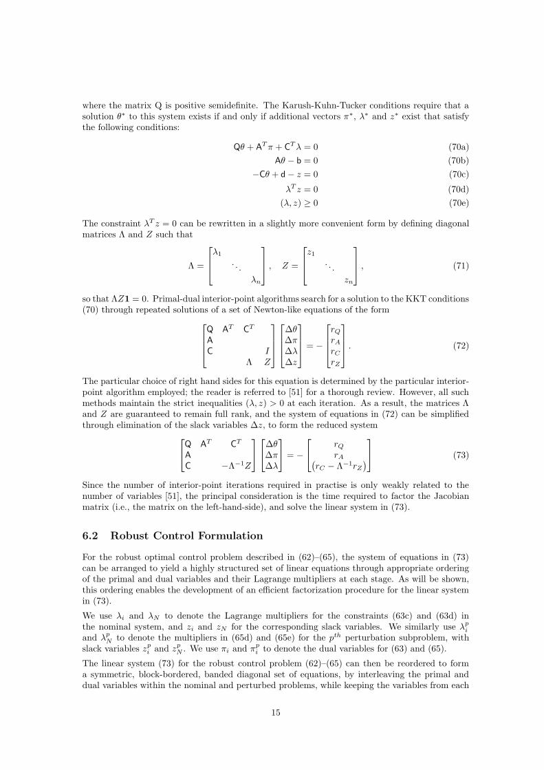
so that ΛZ1 = 0. Primal-dual interior-point algorithms search for a solution to the KKT conditions(70) through repeated solutions of a set of Newton-like equations of the form

Q AT CT

A

C IΛ Z

∆θ∆π∆λ∆z

= −

rQ

rA

rC

rZ

. (72)

The particular choice of right hand sides for this equation is determined by the particular interior-point algorithm employed; the reader is referred to [51] for a thorough review. However, all suchmethods maintain the strict inequalities (λ, z) > 0 at each iteration. As a result, the matrices Λand Z are guaranteed to remain full rank, and the system of equations in (72) can be simplifiedthrough elimination of the slack variables ∆z, to form the reduced system

Q AT CT

A

C −Λ−1Z

∆θ∆π∆λ

= −

rQ

rA(

rC − Λ−1rZ

)

(73)

Since the number of interior-point iterations required in practise is only weakly related to thenumber of variables [51], the principal consideration is the time required to factor the Jacobianmatrix (i.e., the matrix on the left-hand-side), and solve the linear system in (73).

6.2 Robust Control Formulation

For the robust optimal control problem described in (62)–(65), the system of equations in (73)can be arranged to yield a highly structured set of linear equations through appropriate orderingof the primal and dual variables and their Lagrange multipliers at each stage. As will be shown,this ordering enables the development of an efficient factorization procedure for the linear systemin (73).

We use λi and λN to denote the Lagrange multipliers for the constraints (63c) and (63d) inthe nominal system, and zi and zN for the corresponding slack variables. We similarly use λp

i

and λpN to denote the multipliers in (65d) and (65e) for the pth perturbation subproblem, with

slack variables zpi and zp

N . We use πi and πpi to denote the dual variables for (63) and (65).

The linear system (73) for the robust control problem (62)–(65) can then be reordered to forma symmetric, block-bordered, banded diagonal set of equations, by interleaving the primal anddual variables within the nominal and perturbed problems, while keeping the variables from each

15

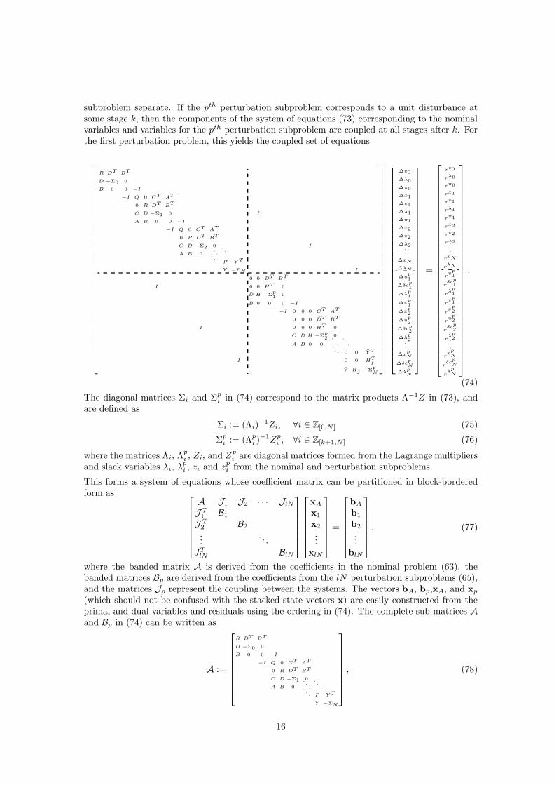
subproblem separate. If the pth perturbation subproblem corresponds to a unit disturbance atsome stage k, then the components of the system of equations (73) corresponding to the nominalvariables and variables for the pth perturbation subproblem are coupled at all stages after k. Forthe first perturbation problem, this yields the coupled set of equations

R DT BT

D −Σ0 0

B 0 0 −I

−I Q 0 CT AT

0 R DT BT

C D −Σ1 0 I

A B 0 0 −I

−I Q 0 CT AT

0 R DT BT

C D −Σ2 0 I

A B 0

...

...

... P Y T

Y −ΣN I

0 0 DT BT

I 0 0 HT 0

D H −Σp1 0

B 0 0 0 −I

−I 0 0 0 CT AT

0 0 0 DT BT

I 0 0 0 HT 0

C D H −Σp2

0

A B 0 0

...

...

... 0 0 Y T

I 0 0 HTf

Y Hf −ΣpN

∆v0

∆λ0

∆π0

∆x1

∆v1

∆λ1

∆π1

∆x2

∆v2

∆λ2...

∆xN

∆λN

∆up1

∆δcp1

∆λp1

∆πp1

∆xp2

∆up2

∆δcp2

∆λp2.

.

.

∆xpN

∆δcpN

∆λpN

=

rv0

rλ0

rπ0

rx1

rv1

rλ1

rπ1

rx2

rv2

rλ2...

rxN

rλN

ru

p1

rδc

p1

rλ

p1

rπ

p1

rx

p2

ru

p2

rδc

p2

rλ

p2.

.

.

rx

pN

rδc

pN

rλ

pN

.

(74)

The diagonal matrices Σi and Σpi in (74) correspond to the matrix products Λ−1Z in (73), and

are defined as

Σi := (Λi)−1Zi, ∀i ∈ Z[0,N ] (75)

Σpi := (Λp

i )−1Zp

i , ∀i ∈ Z[k+1,N ] (76)

where the matrices Λi, Λpi , Zi, and Zp

i are diagonal matrices formed from the Lagrange multipliersand slack variables λi, λp

i , zi and zpi from the nominal and perturbation subproblems.

This forms a system of equations whose coefficient matrix can be partitioned in block-borderedform as

A J1 J2 · · · JlN

J T1 B1

J T2 B2

.... . .

JTlN BlN

xA

x1

x2

...xlN

=

bA

b1

b2

...blN

, (77)

where the banded matrix A is derived from the coefficients in the nominal problem (63), thebanded matrices Bp are derived from the coefficients from the lN perturbation subproblems (65),and the matrices Jp represent the coupling between the systems. The vectors bA, bp,xA, and xp

(which should not be confused with the stacked state vectors x) are easily constructed from theprimal and dual variables and residuals using the ordering in (74). The complete sub-matrices Aand Bp in (74) can be written as

A :=

R DT BT

D −Σ0 0

B 0 0 −I

−I Q 0 CT AT

0 R DT BT

C D −Σ1 0

A B 0

...

...

... P Y T

Y −ΣN

, (78)

16

and

Bp :=

0 0 DT BT

0 0 HT 0

D H −Σpk+1

0

B 0 0 0 −I

−I 0 0 0 CT AT

0 0 0 DT BT

0 0 0 HT 0

C D H −Σpk+2

0

A B 0 0

...

...

... 0 0 Y T

0 0 HTf

Y Hf −ΣpN

. (79)

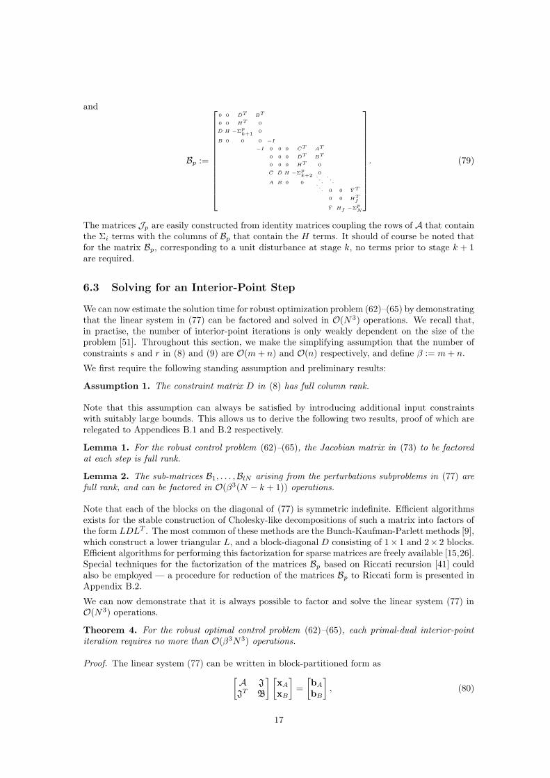
The matrices Jp are easily constructed from identity matrices coupling the rows of A that containthe Σi terms with the columns of Bp that contain the H terms. It should of course be noted thatfor the matrix Bp, corresponding to a unit disturbance at stage k, no terms prior to stage k + 1are required.

6.3 Solving for an Interior-Point Step

We can now estimate the solution time for robust optimization problem (62)–(65) by demonstratingthat the linear system in (77) can be factored and solved in O(N 3) operations. We recall that,in practise, the number of interior-point iterations is only weakly dependent on the size of theproblem [51]. Throughout this section, we make the simplifying assumption that the number ofconstraints s and r in (8) and (9) are O(m + n) and O(n) respectively, and define β := m + n.

We first require the following standing assumption and preliminary results:

Assumption 1. The constraint matrix D in (8) has full column rank.

Note that this assumption can always be satisfied by introducing additional input constraintswith suitably large bounds. This allows us to derive the following two results, proof of which arerelegated to Appendices B.1 and B.2 respectively.

Lemma 1. For the robust control problem (62)–(65), the Jacobian matrix in (73) to be factoredat each step is full rank.

Lemma 2. The sub-matrices B1, . . . ,BlN arising from the perturbations subproblems in (77) arefull rank, and can be factored in O(β3(N − k + 1)) operations.

Note that each of the blocks on the diagonal of (77) is symmetric indefinite. Efficient algorithmsexists for the stable construction of Cholesky-like decompositions of such a matrix into factors ofthe form LDLT . The most common of these methods are the Bunch-Kaufman-Parlett methods [9],which construct a lower triangular L, and a block-diagonal D consisting of 1× 1 and 2× 2 blocks.Efficient algorithms for performing this factorization for sparse matrices are freely available [15,26].Special techniques for the factorization of the matrices Bp based on Riccati recursion [41] couldalso be employed — a procedure for reduction of the matrices Bp to Riccati form is presented inAppendix B.2.

We can now demonstrate that it is always possible to factor and solve the linear system (77) inO(N3) operations.

Theorem 4. For the robust optimal control problem (62)–(65), each primal-dual interior-pointiteration requires no more than O(β3N3) operations.

Proof. The linear system (77) can be written in block-partitioned form as

[

A J

JT B

] [

xA

xB

]

=

[

bA

bB

]

, (80)

17

where the matrix B is block-diagonal with banded blocks Bp, and J :=[

J1 . . . JlN

]

. Ablock-partitioned matrix of this type can be factored and solved as

[

xA

xB

]

=

[

I 0−B−1JT I

] [

∆−1 00 B−1

] [

I −JB−1

0 I

][

bA

bB

]

, (81)

with∆ := (A− JB−1JT ). (82)

where, by virtue of Lemmas 1 and 2, the matrix ∆ is always full rank [25, Thm. 0.8.5].

The structure of the linear system in (77) is quite common [21, 31, 35], and can be solved usingthe following procedure based on Schur complements:

Operation Complexity

factor: Bi = LiDiLTi ∀i ∈ Z[1,lN ] lN · O(β3N) (83a)

∆ = A−

(

lN∑

i=1

JiB−1i J T

i

)

lN · O(β3N2) (83b)

= L∆D∆LT∆ O(β3N3) (83c)

solve: bi = L−Ti (D−1

i (L−1i bi)), ∀i ∈ Z[1,lN ] lN · O(β2N) (83d)

zA = bA −lN∑

i=1

(Jibi), lN · O(βN) (83e)

xA = L−T∆ (D−1

∆ (L−1∆ z)), O(β2N2) (83f)

zi = J Ti xA, ∀i ∈ Z[1,lN ] lN · O(βN) (83g)

xi = bi − L−Ti (D−1

i (L−1i zi)). ∀i ∈ Z[1,lN ] lN · O(β2N) (83h)

Remark 6. It is important to recognize that the order of operations in this solution procedurehas a major influence on its efficiency. In particular, special care is required in forming theproducts JiB

−1i J T

i , particularly when the matrix J Ti is sparse, as many sparse factorization codes

require that the right hand side vectors for a solve of the form B−1i b be posed as dense columns.

We note that, strictly speaking, the proposed method relies on the Riccati factorization techniquediscussed in Appendix B.2 for the factorization of the matrices Bi, rather than factorization intoBi = LiDiL

Ti , though this distinction is not material to our proof. For the formulation in (77)

it is also important to note that since the coupling matrices Ji have no more than a single 1 onevery row and column, matrix products involving left or right multiplication by Ji or J T

i do notrequire any floating point operations to calculate. The reader is referred to [8, App. C] for a morecomplete treatment of complexity analysis for matrix operations.

Remark 7. If the factorization procedure (83) is employed, then the robust optimization problemis an obvious candidate for parallel implementation.

Remark 8. It is not necessary to hand implement the suggested variable interleaving and blockfactorization procedure to realize the suggested block-bordered structure in (77) and O(N 3) be-havior, as any reasonably efficient sparse factorization code may be expected to perform similarsteps automatically; see [15]. Note that the “arrowhead” structure in (77) should be reversed (i.e.pointing down and to the right) in order for direct LDLT factorization to produce sparse factors.

7 Results

Two sparse QP solvers were used to evaluate the proposed formulation. The first, OOQP [19],uses a primal-dual interior-point approach configured with the sparse factorization code MA27

18

from the HSL library [26] and the OOQP version of the multiple-corrector interior-point methodof Gondzio [20].

The second sparse solver used was the QP interface to the PATH [14] solver. This code solvesmixed complementarity problems using an active-set method, and hence can be applied to thestationary conditions of any quadratic program. Note we are dealing with convex QPs, hence eachoptimization problem and its associated complementarity system have equivalent solution sets.

All results reported in this section were generated on a single processor machine, with a 3GhzPentium 4 processor and 1GB of RAM. We restrict our attention to sparse solvers as the amount ofmemory required in the size of the problems considered is prohibitively large for dense factorizationmethods.

A set of test cases was generated to compare the performance of the two sparse solvers using the(M,v) formulation in (45) with the decomposition based method of Section 5. Each test case isdefined by its number of states n and horizon length N . The remaining problem parameters werechosen using the following rules:

• There are twice as many states as inputs.

• The constraint sets W , Z and Xf represent randomly selected symmetric bounds on thestates and inputs subjected to a random similarity transformation.

• The states space matrices A and B are randomly generated, with (A, B) controllable, andA stable.

• The dimension l of the generating disturbance is chosen as half the number of states, withrandomly generated E of full column rank.

• All test cases have feasible solutions. The current state is selected such that at least someof the inequality constraints in (63c) are active at the optimal solution.

The average computational times required by each of the two solvers for the two problem formu-lations for a range of problem sizes are shown in Table 1. Each entry represents the average of tentest cases, unless otherwise noted.

It is clear from these results that, as expected, the decomposition-based formulation can be solvedmuch more efficiently than the original (M,v) formulation for the robust optimal control problemin every case, and that the difference in solution times increases dramatically with increasedproblem size. Additionally, the decomposition formulation seems particularly well suited to theinterior-point solver (OOQP), rather than the active set method (PATH). Nevertheless we expectthe performance of active set methods to improve relative to interior-point methods when solvinga sequence of similar QPs that would occur in predictive control, i.e., when a good estimate ofthe optimal active set is available at the start of computation. That is, interior-point methods areparticulary effective in “cold start” situations, while the efficiency of active set methods is likelyto improve given a “warm start”. As is common in interior-point methods, we find that the actualnumber of iterations required for solution of each problem type in Table 1 is nearly constant withincreasing horizon length.

Figure 1 shows that the interior-point solution time increases cubicly with horizon length fora randomly generated problem with 4 states. The performance closely matches the predictedbehavior described in Section 5. For the particular problem shown, the number of iterationsrequired for the OOQP algorithm to converge increased from 9 to 11 over the range of horizonlengths considered.

19

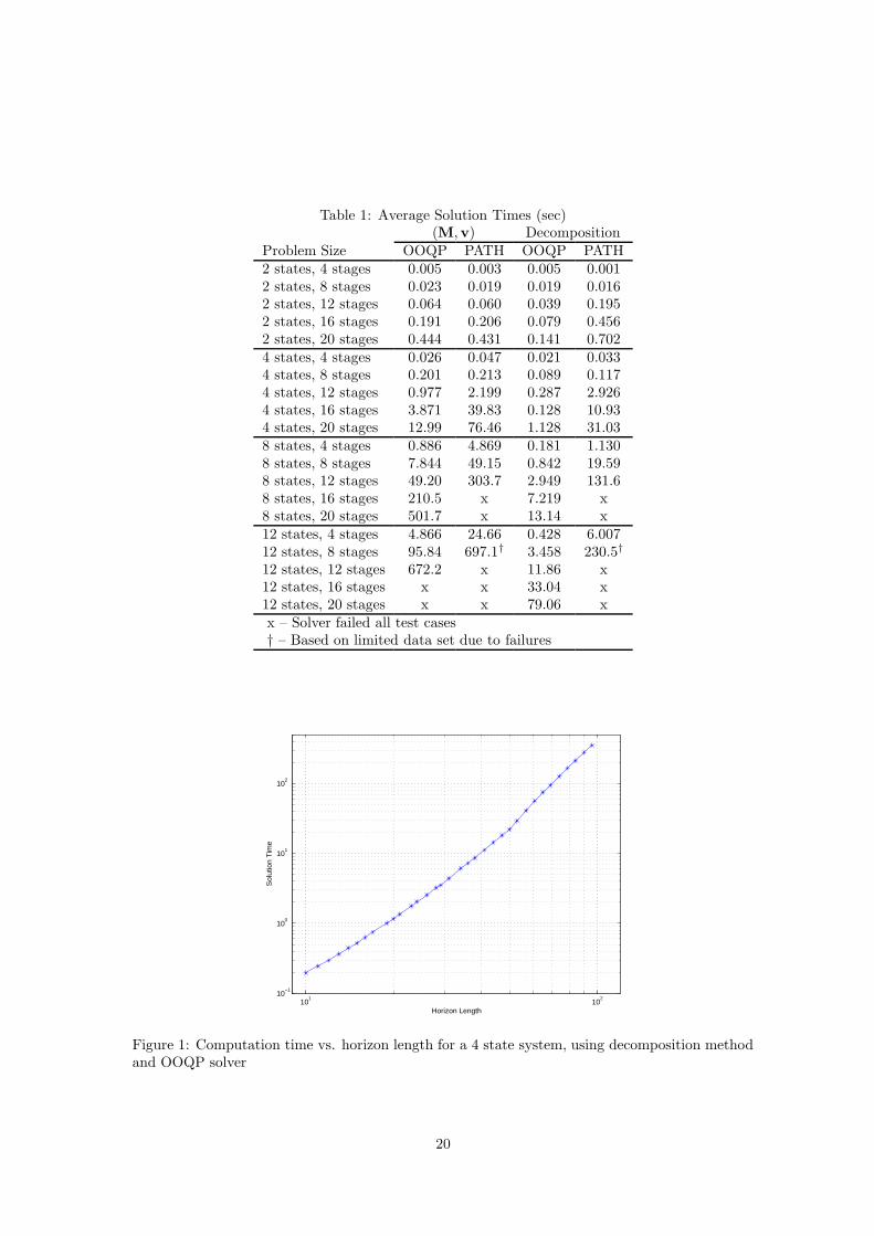
Table 1: Average Solution Times (sec)(M,v) Decomposition

Problem Size OOQP PATH OOQP PATH2 states, 4 stages 0.005 0.003 0.005 0.0012 states, 8 stages 0.023 0.019 0.019 0.0162 states, 12 stages 0.064 0.060 0.039 0.1952 states, 16 stages 0.191 0.206 0.079 0.4562 states, 20 stages 0.444 0.431 0.141 0.7024 states, 4 stages 0.026 0.047 0.021 0.0334 states, 8 stages 0.201 0.213 0.089 0.1174 states, 12 stages 0.977 2.199 0.287 2.9264 states, 16 stages 3.871 39.83 0.128 10.934 states, 20 stages 12.99 76.46 1.128 31.038 states, 4 stages 0.886 4.869 0.181 1.1308 states, 8 stages 7.844 49.15 0.842 19.598 states, 12 stages 49.20 303.7 2.949 131.68 states, 16 stages 210.5 x 7.219 x8 states, 20 stages 501.7 x 13.14 x12 states, 4 stages 4.866 24.66 0.428 6.00712 states, 8 stages 95.84 697.1† 3.458 230.5†

12 states, 12 stages 672.2 x 11.86 x12 states, 16 stages x x 33.04 x12 states, 20 stages x x 79.06 xx – Solver failed all test cases† – Based on limited data set due to failures

101

102

10−1

100

101

102

Horizon Length

Sol

utio

n T

ime

Figure 1: Computation time vs. horizon length for a 4 state system, using decomposition methodand OOQP solver

20

8 Conclusions and Future Work

We have derived a highly efficient computational method for calculation of affine-state feedbackpolicies for robust control of constrained systems with bounded disturbances. This is done byexploiting the structure of the underlying optimization problem and deriving an equivalent problemwith considerable structure and sparsity, resulting in a problem formulation that is particularlysuited to an interior-point solution method. As a result, robustly stabilizing receding horizoncontrol laws based on optimal state-feedback policies have become practically realizable, even forsystems of significant size or with long horizon lengths.

In Section 6 we proved that, when applying an interior-point solution technique to our robustoptimal control problem, each iteration of the method can be solved using a number of operationsproportional to the cube of the control horizon length. We appeal to the Riccati based factorizationtechnique in [41] to support this claim. However, we stress that the results in Section 7, whichdemonstrate this cubic-time behavior numerically, are based on freely available optimization andlinear algebra packages and do not rely on any special factorization methods.

A number of open research issues remain. It may be possible to possible to further exploit thestructure of our control problem by developing specialized factorization algorithms for the factor-ization of each interior-point step, e.g. through the parallel block factorization procedure alludedto in Remark 7. It may also be possible to achieve considerably better performance by placingfurther constraints on the structure of the disturbance feedback matrix M, though this appearsdifficult to do if the attractive invariance and stability properties of the present formulation areto be preserved.

Many of the system-theoretic results developed in [22] hold for a fairly broad classes of disturbancesand cost functions. For example, when the disturbance is Guassian the problem may be modifiedto require that the state and input constraints hold with a certain pre-specified probability, and theprobabilistic constraints converted to second-order cone constraints [8, pp. 157–8]. Alternatively,the cost function for the finite horizon control problem may require the minimization of the finite-horizon `2 gain of a system [28]. In all of these cases, there is a strong possibility that theunderlying problem structure may be exploited to realise a substantial increase in computationalefficiency.

References

[1] B. D. O. Anderson and J. B. Moore. Optimal control: linear quadratic methods. Prentice-Hall,Inc., Upper Saddle River, NJ, USA, 1990.

[2] A. Bemporad. Reducing conservativeness in predictive control of constrained systems withdisturbances. In Proc. 37th IEEE Conf. on Decision and Control, pages 1384–1391, Tampa,FL, USA, December 1998.

[3] A. Bemporad and M. Morari. Robust Model Predictive Control: A Survey in Robustness inIdentification and Control, volume 245 of Lecture Notes in Control and Information Sciences,pages 207–226. Ed. A. Garulli, A. Tesi, and A. Vicino. Springer-Verlag, 1999.

[4] A. Ben-Tal, A. Goryashko, E. Guslitzer, and A. Nemirovski. Adjustable robust solutions ofuncertain linear programs. Technical report, Minerva Optimization Center, Technion, IsraeliInstitute of Technology, 2002.

[5] D. P. Bertsekas and I. B. Rhodes. Sufficiently informative functions and the minimax feed-back control of uncertain dynamic systems. IEEE Transactions on Automatic Control, AC-18(2):117–124, April 1973.

21

[6] L. Biegler. Efficient solution of dynamic optimization and NMPC problems. In F. Allgowerand A. Zheng, editors, Nonlinear Model Predictive Control, volume 26 of Progress in Systemsand Control Theory, pages 219–243. Birkhauser, 2000.

[7] F. Blanchini. Set invariance in control. Automatica, 35(1):1747–1767, November 1999.

[8] S. Boyd and L. Vandenberghe. Convex Optimization. Cambridge University Press, 2004.

[9] J. R. Bunch, L. Kaufman, and B. N. Parlett. Decomposition of a symmetric matrix. Nu-merische Mathematik, 27:95–110, 1976.

[10] E.F. Camacho and C. Bordons. Model Predictive Control. Springer, second edition, 2004.

[11] L. Chisci, J. A. Rossiter, and G. Zappa. Systems with persistent state disturbances: predictivecontrol with restricted constraints. Automatica, 37(7):1019–1028, July 2001.

[12] M.A. Dahleh and I.J. Diaz-Bobillo. Control of Uncertain Systems. Prentice Hall, 1995.

[13] M. Diehl, H. G. Bock, and J. P. Schloder. A real-time iteration scheme for nonlinear optimiza-tion in optimal feedback control. SIAM Journal on Control and Optimization, 43(5):1714–1736, 2005.

[14] S. P. Dirske and M. C. Ferris. The PATH solver: A non-monotone stabilization scheme formixed complementarity problems. Optimization Methods and Software, 5:123–156, 1995.

[15] I.S. Duff, A.M. Erisman, and J.K. Reid. Direct Methods for Sparse Matrices. Oxford Univer-sity Press, Oxford, England, 1986.

[16] G. E. Dullerud and F. Paganini. A Course in Robust Control Theory: A Convex Approach.Springer-Verlag, New York, 2000.

[17] I. J. Fialho and T. T. Georgiou. `1 state-feedback control with a prescribed rate of exponentialconvergence. IEEE Transactions on Automatic Control, 42(10):1476–81, October 1997.

[18] S. J. Gartska and R. J-B. Wets. On decisions rules in stochastic programming. MathematicalProgramming, 7:117–143, 1974.

[19] E. M. Gertz and S. J. Wright. Object-oriented software for quadratic programming”. ACMTransactions on Mathematical Software, 29:58–81, 2003.

[20] J. Gondzio. Multiple centrality corrections in a primal-dual method for linear programming.Computational Optimization and Applications, 6:137–156, 1996.

[21] J. Gondzio and A. Grothey. Parallel interior point solver for structured quadratic programs:Application to financial planning problems. Technical Report MS-03-001, School of Mathe-matics, The University of Edinburgh, December 2003.

[22] P. J. Goulart, E. C. Kerrigan, and J. M. Maciejowski. Optimization over state feedback poli-cies for robust control with constraints. Automatica, 2006. Accepted. Available as TechnicalReport CUED/F-INFENG/TR.494, Cambridge University Engineering Department, March2005. Available from http://www-control.eng.cam.ac.uk/.

[23] M. Green and D. J. N. Limebeer. Linear Robust Control. Prentice Hall, 1995.

[24] E. Guslitser. Uncertainty-immunized solutions in linear programming. Master’s thesis, Tech-nion, Israeli Institute of Technology, June 2002.

[25] R.A. Horn and C.R. Johnson. Matrix Analysis. Cambridge University Press, 1985.

[26] HSL. HSL 2002: A collection of Fortran codes for large scale scientific computation.www.cse.clrc.ac.uk/nag/hsl, 2002.

22

[27] D.H. Jacobson and D.Q. Mayne. Differential Dynamic Programming. Elsevier, New York,NY, USA, 1970.

[28] E. C. Kerrigan and T. Alamo. A convex parameterization for solving constrained min-maxproblems with a quadratic cost. In Proc. 2004 American Control Conference, Boston, MA,USA, June 2004.

[29] E. C. Kerrigan and J. M. Maciejowski. On robust optimization and the optimal control ofconstrained linear systems with bounded state disturbances. In Proc. 2003 European ControlConference, Cambridge, UK, September 2003, 2003.

[30] E. C. Kerrigan and J. M. Maciejowski. Properties of a new parameterization for the control ofconstrained systems with disturbances. In Proc. 2004 American Control Conference, Boston,MA, USA, June 2004.

[31] D. P. Koester. Parallel Block-Diagonal-Bordered Sparse Linear Solvers for Power SystemsApplications. PhD thesis, Syracuse University, October 1995.

[32] Y. I. Lee and B. Kouvaritakis. Constrained receding horizon predictive control for systemswith disturbances. International Journal of Control, 72(11):1027–1032, August 1999.

[33] J. Lofberg. Approximations of closed-loop MPC. In Proc. 42nd IEEE Conference on Decisionand Control, pages 1438–1442, Maui, Hawaii, USA, December 2003.

[34] J. Lofberg. Minimax Approaches to Robust Model Predictive Control. PhD thesis, LinkopingUniversity, Apr 2003.

[35] L. G. Khachiyan M. D. Grigoriadis. An interior point method for bordered block-diagonallinear programs. SIAM Journal on Optimization, 6(4):913–932, 1996.

[36] J. M. Maciejowski. Predictive Control with Constraints. Prentice Hall, UK, 2002.

[37] D. Q. Mayne. Control of constrained dynamic systems. European Journal of Control, 7:87–99,2001. Survey paper.

[38] D. Q. Mayne, J. B. Rawlings, C. V. Rao, and P. O. M. Scokaert. Constrained model predictivecontrol: Stability and optimality. Automatica, 36(6):789–814, June 2000. Survey paper.

[39] D. Q. Mayne, M. M. Seron, and S. V. Rakovic. Robust model predictive control of constrainedlinear systems with bounded disturbances. Automatica, 41(2):219–24, February 2005.

[40] S. J. Qin and T. A. Badgwell. A survey of industrial model predictive control technology.Control Engineering Practice, 11:733–764, 2003.

[41] C. V. Rao, S. J. Wright, and J. B. Rawlings. Application of interior–point methods to modelpredictive control. Journal of Optimization Theory and Applications, 99:723–757, 1998.

[42] R. T. Rockafellar and R. J-B. Wets. Variational Analysis. Springer-Verlag, 1998.

[43] P. O. M. Scokaert and D. Q. Mayne. Min-max feedback model predictive control for con-strained linear systems. IEEE Transactions on Automatic Control, 43(8):1136–1142, August1998.

[44] J. S. Shamma. Optimization of the `∞-induced norm under full state feedback. IEEE Trans-actions on Automatic Control, 41(4):533–44, April 1996.

[45] G. Stein. Respect the unstable. IEEE Control Systems Magazine, 34(4):12–25, August 2003.

[46] M. Sznaier. Mixed l1/H∞ control of MIMO systems via convex optimization. IEEE Trans-actions on Automatic Control, 43(9):1229–1241, September 1998.

23

[47] D. H. van Hessem. The ISS philosophy as a unifying framework for stability-like behavior.PhD thesis, Technical University of Delft, June 2004.

[48] D. H. van Hessem and O. H. Bosgra. A conic reformulation of model predictive controlincluding bounded and stochastic disturbances under state and input constraints. In Proc.41st IEEE Conference on Decision and Control, pages 4643–4648, December 2002.

[49] H. S. Witsenhausen. A minimax control problem for sampled linear systems. IEEE Transac-tions on Automatic Control, AC-13(1):5–21, 1968.

[50] S. J. Wright. Interior point methods for optimal control of discrete-time systems. J. Optim.Theory Appls, 77:161–187, 1993.

[51] S. J. Wright. Primal-Dual Interior-Point Methods. SIAM Publications, Philadelphia, 1997.

[52] G. Zames. Feedback and optimal sensitivity: Model reference transformations, multiplica-tive seminorms, and approximate inverses. IEEE Transactions on Automatic Control, AC-26(2):301–320, April 1981.

[53] K. Zhou, J. Doyle, and K. Glover. Robust and Optimal Control. Prentice-Hall, 1996.

A Matrix Definitions

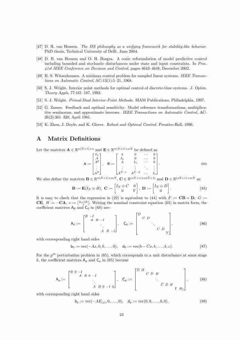
Let the matrices A ∈ Rn(N+1)×n and E ∈ R

n(N+1)×nN be defined as

A :=

2

6

6

6

6

6

4

In

AA2

.

..AN

3

7

7

7

7

7

5

, E :=

2

6

6

6

6

6

4

0 0 · · · 0In 0 · · · 0A In · · · 0...

..

.. . .

..

.AN−1 AN−2 · · · In

3

7

7

7

7

7

5

. (84)

We also define the matrices B ∈ Rn(N+1)×mN , C ∈ R

(sN+r)×n(N+1) and D ∈ R(sN+r)×mN as

B := E(IN ⊗ B), C :=

[

IN ⊗ C 00 Y

]

, D :=

[

IN ⊗ D0

]

. (85)

It is easy to check that the expression in (22) is equivalent to (44) with F := CB + D, G :=CE, H := −CA, c := [ 1N⊗b

z ]. Writing the nominal constraint equation (63) in matrix form, thecoefficient matrices A0 and C0 in (68) are:

A0 :=

B −IA B −I

. . .

A B −I

, C0 :=

DC D

. . .

C DY

, (86)

with corresponding right hand sides

b0 := vec(−Ax, 0, 0, . . . , 0), d0 := vec(b − Cx, b, . . . , b, z). (87)

For the pth perturbation problem in (65), which corresponds to a unit disturbance at some stagek, the coefficient matrices Ap and Cp in (65) become

Ap :=

B 0 −IA B 0 −I

. . .

A B 0 −I 0

, Cp :=

D HC D H

. . .

C D HY Hf

, (88)

with corresponding right hand sides

bp := vec(−AE(j), 0, . . . , 0), dp := vec(0, 0, . . . , 0, 0). (89)

24

B Rank of the Jacobian and Reduction to Riccati Form

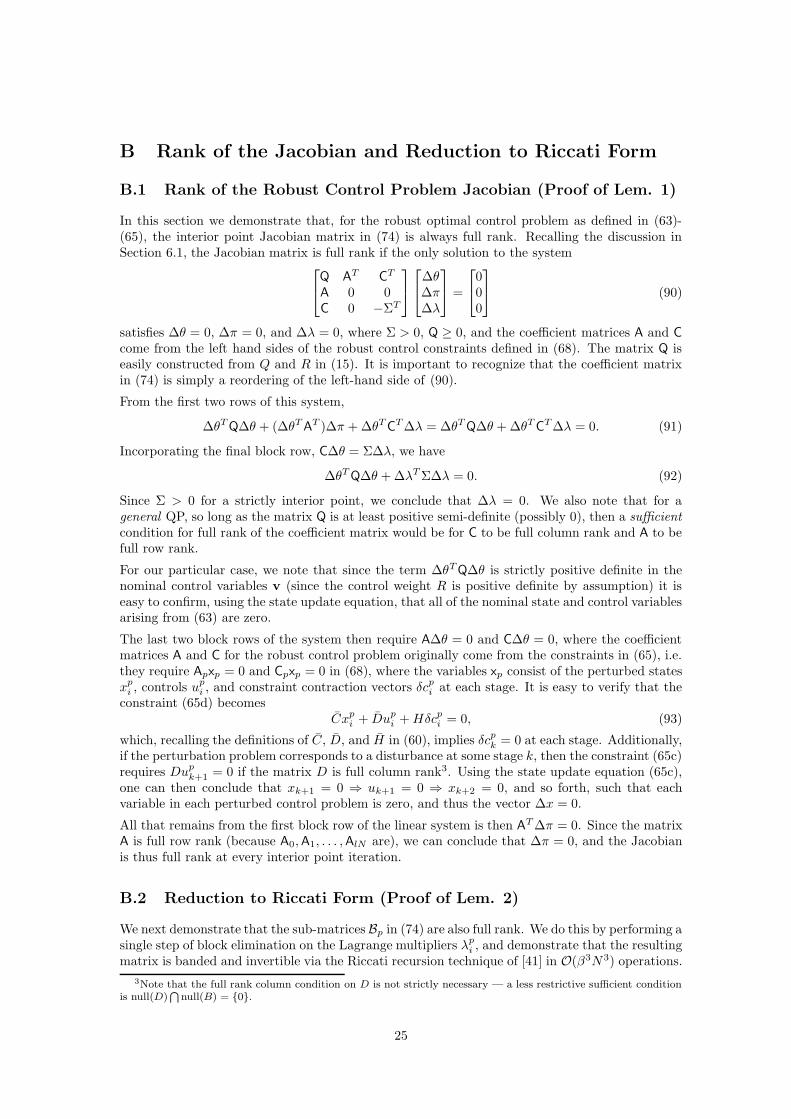
B.1 Rank of the Robust Control Problem Jacobian (Proof of Lem. 1)

In this section we demonstrate that, for the robust optimal control problem as defined in (63)-(65), the interior point Jacobian matrix in (74) is always full rank. Recalling the discussion inSection 6.1, the Jacobian matrix is full rank if the only solution to the system

Q AT CT

A 0 0C 0 −ΣT

∆θ∆π∆λ

=

000

(90)

satisfies ∆θ = 0, ∆π = 0, and ∆λ = 0, where Σ > 0, Q ≥ 0, and the coefficient matrices A and C

come from the left hand sides of the robust control constraints defined in (68). The matrix Q iseasily constructed from Q and R in (15). It is important to recognize that the coefficient matrixin (74) is simply a reordering of the left-hand side of (90).

From the first two rows of this system,

∆θT Q∆θ + (∆θT AT )∆π + ∆θT CT ∆λ = ∆θT Q∆θ + ∆θT CT ∆λ = 0. (91)

Incorporating the final block row, C∆θ = Σ∆λ, we have

∆θT Q∆θ + ∆λT Σ∆λ = 0. (92)

Since Σ > 0 for a strictly interior point, we conclude that ∆λ = 0. We also note that for ageneral QP, so long as the matrix Q is at least positive semi-definite (possibly 0), then a sufficientcondition for full rank of the coefficient matrix would be for C to be full column rank and A to befull row rank.

For our particular case, we note that since the term ∆θT Q∆θ is strictly positive definite in thenominal control variables v (since the control weight R is positive definite by assumption) it iseasy to confirm, using the state update equation, that all of the nominal state and control variablesarising from (63) are zero.

The last two block rows of the system then require A∆θ = 0 and C∆θ = 0, where the coefficientmatrices A and C for the robust control problem originally come from the constraints in (65), i.e.they require Apxp = 0 and Cpxp = 0 in (68), where the variables xp consist of the perturbed statesxp

i , controls upi , and constraint contraction vectors δcp

i at each stage. It is easy to verify that theconstraint (65d) becomes

Cxpi + Dup

i + Hδcpi = 0, (93)

which, recalling the definitions of C, D, and H in (60), implies δcpk = 0 at each stage. Additionally,

if the perturbation problem corresponds to a disturbance at some stage k, then the constraint (65c)requires Dup

k+1 = 0 if the matrix D is full column rank3. Using the state update equation (65c),one can then conclude that xk+1 = 0 ⇒ uk+1 = 0 ⇒ xk+2 = 0, and so forth, such that eachvariable in each perturbed control problem is zero, and thus the vector ∆x = 0.

All that remains from the first block row of the linear system is then AT ∆π = 0. Since the matrixA is full row rank (because A0, A1, . . . , AlN are), we can conclude that ∆π = 0, and the Jacobianis thus full rank at every interior point iteration.

B.2 Reduction to Riccati Form (Proof of Lem. 2)

We next demonstrate that the sub-matrices Bp in (74) are also full rank. We do this by performing asingle step of block elimination on the Lagrange multipliers λp

i , and demonstrate that the resultingmatrix is banded and invertible via the Riccati recursion technique of [41] in O(β3N3) operations.

3Note that the full rank column condition on D is not strictly necessary — a less restrictive sufficient conditionis null(D)

T

null(B) = {0}.

25

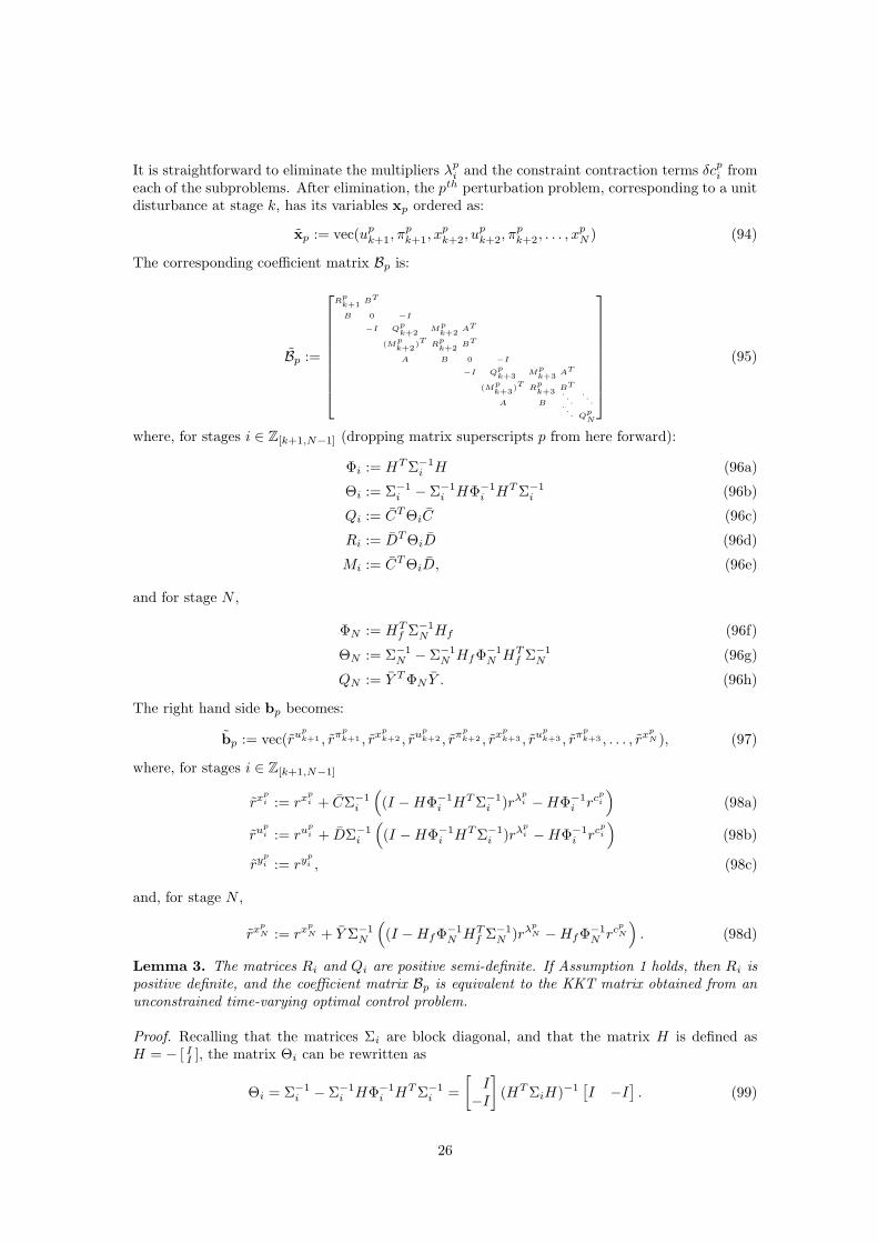
It is straightforward to eliminate the multipliers λpi and the constraint contraction terms δcp

i fromeach of the subproblems. After elimination, the pth perturbation problem, corresponding to a unitdisturbance at stage k, has its variables xp ordered as:

xp := vec(upk+1, π

pk+1, x

pk+2, u

pk+2, π

pk+2, . . . , x

pN ) (94)

The corresponding coefficient matrix Bp is:

Bp :=

Rpk+1

BT

B 0 −I

−I Qpk+2

Mpk+2

AT

(Mpk+2

)TR

pk+2

BT

A B 0 −I

−I Qpk+3

Mpk+3

AT

(Mpk+3

)T Rpk+3

BT

A B

...

...

... Q

pN

(95)

where, for stages i ∈ Z[k+1,N−1] (dropping matrix superscripts p from here forward):

Φi := HT Σ−1i H (96a)

Θi := Σ−1i − Σ−1

i HΦ−1i HT Σ−1

i (96b)

Qi := CT ΘiC (96c)

Ri := DT ΘiD (96d)

Mi := CT ΘiD, (96e)

and for stage N ,

ΦN := HTf Σ−1

N Hf (96f)

ΘN := Σ−1N − Σ−1

N HfΦ−1N HT

f Σ−1N (96g)

QN := Y T ΦN Y . (96h)

The right hand side bp becomes:

bp := vec(rup

k+1 , rπp

k+1 , rxp

k+2 , rup

k+2 , rπp

k+2 , rxp

k+3 , rup

k+3 , rπp

k+3 , . . . , rxp

N ), (97)

where, for stages i ∈ Z[k+1,N−1]

rxpi := rx

pi + CΣ−1

i

(

(I − HΦ−1i HT Σ−1

i )rλpi − HΦ−1

i rcpi

)

(98a)

rupi := ru

pi + DΣ−1

i

(

(I − HΦ−1i HT Σ−1

i )rλpi − HΦ−1

i rcpi

)

(98b)

rypi := ry

pi , (98c)

and, for stage N ,

rxp

N := rxp

N + Y Σ−1N

(

(I − HfΦ−1N HT

f Σ−1N )rλ

p

N − HfΦ−1N rc

p

N

)

. (98d)

Lemma 3. The matrices Ri and Qi are positive semi-definite. If Assumption 1 holds, then Ri ispositive definite, and the coefficient matrix Bp is equivalent to the KKT matrix obtained from anunconstrained time-varying optimal control problem.

Proof. Recalling that the matrices Σi are block diagonal, and that the matrix H is defined asH = − [ I

I ], the matrix Θi can be rewritten as

Θi = Σ−1i − Σ−1

i HΦ−1i HT Σ−1

i =

[

I−I

]

(HT ΣiH)−1[

I −I]

. (99)

26

This can be verified by partitioning the matrices in (99) into 2 × 2 blocks. If the matrix Σi is

partitioned as Σi :=[

Σi,1 00 Σi,2

]

, then (99) is equivalent to

[

Σ−1i,1 − Σ−1

i,1 (Σ−1i,1 + Σ−1

i,2 )−1Σ−1i,1 −Σ−1

i,1 (Σ−1i,1 + Σ−1

i,2 )−1Σ−1i,2

−Σ−1i,2 (Σ−1

i,1 + Σ−1i,2 )−1Σ−1

i,1 Σ−1i,1 − Σ−1

i,2 (Σ−1i,1 + Σ−1

i,2 )−1Σ−1i,2

]

=

[

I−I

]

(Σ−1i,1 +Σ−1

i,2 )−1[

I −I]

which is easily verified using standard matrix identities. It then follows that Ri is positive semi-definite, since it may be written as

Ri = DT

[

I−I

]

(HT ΣiH)−1[

I −I]

D (100)

= 4DT (Σi,1 + Σi,2)−1D ≥ 0 (101)

which is clearly positive definite if D is full column rank. A similar argument establishes the resultfor Qi. We note that it is always possible to force C and D to be full column rank through theintroduction of redundant constraints with very large upper bounds. The matrix Bp is equivalentto the KKT matrix for the problem:

minuk+1,...,uN−1,

xk+1,...,xN

N−1∑

i=(k+1)

1

2(‖xi‖

2Q + ‖ui‖

2R + 2xiMiui) +

1

2‖xN‖2

Q (102)

subject to:

xk = E(j), (103a)

xi+1 = Axi + Bui, ∀i ∈ Z[k+1,N−1], (103b)

which can be solved via Riccati recursion in O(N−k+1) operations if the matrices Ri are positivedefinite [41].

Remark 9. The coefficient matrix Bp in (95) can be factored in O((N−k+1)(m+n)3) operationsusing the Riccati recursion procedure proposed in [41] if the matrices Ri are positive definite. Anadditional O((N − k + 1)(m + n)2) operations are required for the solution of each right hand side.We note that in [41] the Riccati factorization procedure is shown to be numerically stable, and thatsimilar arguments can be used to show that factorization of (95) is also stable. We omit detailsof this for brevity.

B.3 Complete Reduced Problem

Finally, we verify that the variable eliminations of the preceding section have not disrupted thebordered block diagonal structure of the Jacobian matrix in (74). After elimination in each of theperturbation subproblems, the coefficient matrix A for the nominal problem becomes:

A :=

R DT BT

D −Σ0 0

B 0 0 −I

−I Q 0 CT AT

0 R DT BT

C D −Σ1 0

A B 0

...

...

... Qf Y T

Y −ΣN

(104)

with variable ordering and corresponding right hand side:

xA := vec(v0, λ0, y0, x1, v1, λ1, y1, . . . , xN , N) (105)

bA := vec(rv0 , rλ0 , ry0 , rx1 , rv1 , rλ1 , ry1 , . . . , rxN , rλN ), (106)

27

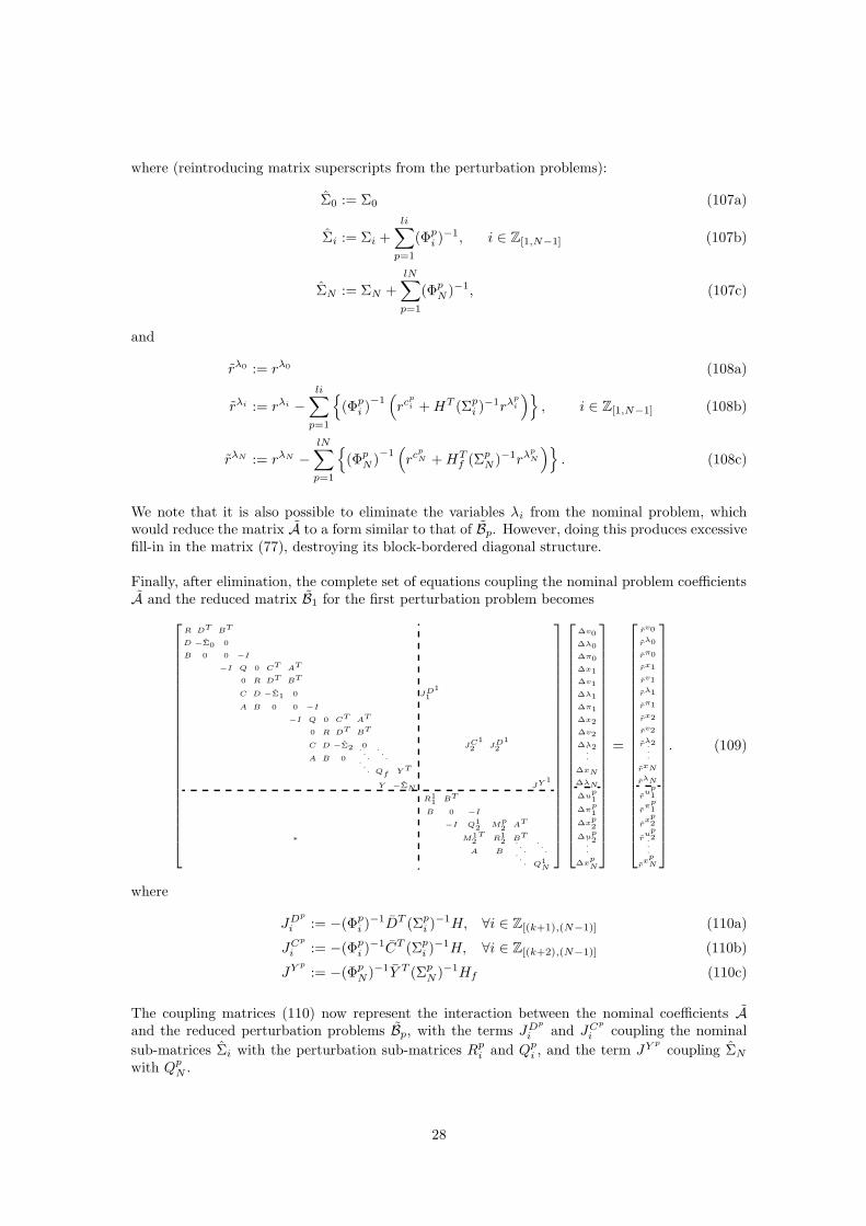
where (reintroducing matrix superscripts from the perturbation problems):

Σ0 := Σ0 (107a)

Σi := Σi +li∑

p=1

(Φpi )

−1, i ∈ Z[1,N−1] (107b)

ΣN := ΣN +

lN∑

p=1

(ΦpN )−1, (107c)

and

rλ0 := rλ0 (108a)

rλi := rλi −li∑

p=1

{

(Φpi )

−1(

rcpi + HT (Σp

i )−1rλ

pi

)}

, i ∈ Z[1,N−1] (108b)

rλN := rλN −lN∑

p=1

{

(ΦpN )

−1(

rcp

N + HTf (Σp

N )−1rλp

N

)}

. (108c)

We note that it is also possible to eliminate the variables λi from the nominal problem, whichwould reduce the matrix A to a form similar to that of Bp. However, doing this produces excessivefill-in in the matrix (77), destroying its block-bordered diagonal structure.

Finally, after elimination, the complete set of equations coupling the nominal problem coefficientsA and the reduced matrix B1 for the first perturbation problem becomes

R DT BT

D −Σ0 0

B 0 0 −I

−I Q 0 CT AT

0 R DT BT

C D −Σ1 0 JD11

A B 0 0 −I

−I Q 0 CT AT

0 R DT BT

C D −Σ2 0 JC12 JD1

2

A B 0

...

...

... Qf Y T

Y −ΣN JY 1

R11 BT

B 0 −I

−I Q12 M

p2

AT

∗ M12

TR1

2 BT

A B

...

...

... Q1

N

∆v0

∆λ0

∆π0

∆x1

∆v1

∆λ1

∆π1

∆x2

∆v2

∆λ2...

∆xN

∆λN

∆up1

∆πp1

∆xp2

∆up2.

.

.

∆xpN

=

rv0

rλ0

rπ0

rx1

rv1

rλ1

rπ1

rx2

rv2

rλ2...

rxN

rλN

ru

p1

rπ

p1

rx

p2

ru

p2.

.

.

rx

pN

. (109)

where

JDp

i := −(Φpi )

−1DT (Σpi )

−1H, ∀i ∈ Z[(k+1),(N−1)] (110a)

JCp

i := −(Φpi )

−1CT (Σpi )

−1H, ∀i ∈ Z[(k+2),(N−1)] (110b)

JY p

:= −(ΦpN)−1Y T (Σp

N )−1Hf (110c)

The coupling matrices (110) now represent the interaction between the nominal coefficients Aand the reduced perturbation problems Bp, with the terms JDp

i and JCp

i coupling the nominal

sub-matrices Σi with the perturbation sub-matrices Rpi and Qp

i , and the term JY p

coupling ΣN

with QpN .

28