Finite horizon robust model predictive control with

terminal cost constraints

Danlei Chu, Tongwen Chen and Horacio J. Marquez ∗

Department of Electrical & Computer Engineering,University of Alberta, Canada, T6G 2V4

Abstract

In this paper, we develop a finite horizon model predictive control algorithm which

is robust to modelling uncertainties. A moving average system matrix is constructed to

capture modelling uncertainties and facilitate the future output prediction. The paper is

mainly focused on the step tracking problem. Using linear matrix inequality techniques, the

design is converted into a semi-definite optimization problem. Closed-loop stability, known

to be one of the most challenging topics in finite horizon model predictive control, is treated

by adding extra terminal cost constraints in the semi-definite optimization. A simulation

example demonstrates that the approach can be useful for practical applications.

1 Introduction

Since the first version of model predictive control (MPC), known as dynamic matrix control

(DMC), was published in 1978, various MPC algorithms have been developed in the past two

decades [1, 2, 3]; for example, generalized predictive control (GPC) designed for stochastic sys-

tems, predictive function control (PFC) capable of handling non-linear and unstable processes,

and internal model predictive control (IMC) which guarantees closed-loop stability. All such

schemes are featured with a critical property of combining input/output constraints with MPC

formulation explicitly, which enables MPC to be widely accepted in petro-chemical, automotive,

food processing, metallurgy, and other industries [4]. Most versions of MPC adopt a common

assumption, namely, setting system models precisely (so-called nominal models) and neglecting

all internal and external ubiquitous uncertainties. The assumption simplifies MPC formulation

dramatically, but may impair the controller performance and/or closed-loop stability. Nor-

mally, the standard MPC process is composed of three steps: future state/output prediction,∗Corresponding author. Tel.: +1-780-492-3334, Fax.: +1-780-492-1811

Email address: marquez@ece.ualberta.ca (Horacio J. Marquez)

1

objective function optimization, and control signal implementation. The accuracy in the three

steps is highly dependent on the model precision. A small parameter perturbation may lead to

constraint violation or unstable regulation. To overcome such a limitation, it is necessary to

study robust model predictive control (RMPC) by incorporating model uncertainties into the

design.

The barriers of the extension of tradition MPC strategies to robust cases lie in two aspects:

one is state/output predictions and the other is closed-loop stability. For the former, researchers

tend to utilize the uncertainty configuration to facilitate future state/output expression, and

for the latter, employ the invariant set theorem to guarantee the state/output convergence in

the presence of system uncertainties. The min-max optimization, as a quite mature technique,

has been used to analyze RMPC problems in the late 1990’s [6, 5, 7]. Briefly speaking, given

a structured objective function, which is usually defined in the form of the weighted 2-norm

summation, maximize the objective based on the definition of system uncertainties, derive an

upper bound of the objective, and then minimize the bound with respect to manipulated in-

puts. Campo and Morari [8], Lee and Yu [9], Bemporad and Morari [7], and Lee and Cooley

[10] independently introduced min-max into the RMPC formulation. In 1996, Kothare and

co-workers [11], based on the min-max strategy, established a successful infinite horizon robust

model predictive control (IH-RMPC) algorithm, which dramatically decreased the computa-

tional complexity and increased the implementation efficiency. Two structured uncertainty

frameworks, namely, polytopic and structured feedback uncertainties [12], were covered in this

paper. The IH-RMPC design was converted to a standard semi-definite optimization problem

[13], which was featured with linear objective functions and linear matrix inequality (LMI)

constraints. The key point of this approach is the derivation of an auxiliary quadratic functions

of predicted states and an upper bound of the objective. Consequently, future state/output

predictions are avoided skillfully. From the characteristics of linear matrix inequalities (LMI),

fast convergence and polynomial complexity, IH-RMPC is known as one of the most effective

regulations in the robust process control area. Since then IH-RMPC has drawn considerable

attention in the literature: Rodrigues and Odloak developed an output-tracking IH-RMPC al-

gorithm [14]; Wan and Kothare derived an off-line IH-RMPC formulation problem [15]; and Hu

and Linnemann extended the IH-RMPC scheme into nonlinear cases [16]. They all inherited

the effectiveness of LMI techniques, and guaranteed closed-loop stability. Moreover, associated

2

by terminal constraints or deriving a state invariant set, the upper bound of the objective

function was employed as a Lyapunov function and enforced to converge while MPC iteration.

Although IH-RMPC possesses superiority as viewed from stability and efficiency, it limits the

system tuning freedoms, and feasibility is another potential problem [17].

Compared with traditional MPC schemes, IH-RMPC can not use prediction horizon Np

and control horizon Nu as tuning parameters to achieve the trade off between system stability

and performance (actually for nominal cases, these two parameters are quite effective tuning

approaches [18]). On the other hand, IH-RMPC always presumes that there exists a unique

control policy which leads to the expected performance in all possible uncertain situations

throughout entire infinite horizons. The condition may result in low performance solutions and

even infeasibility problems [6, 19]. Therefore the development of FH-RMPC is necessary as

well as natural. From the above discussion, we believe that the main obstacle of FH-RMPC

comes from the computational complexity of future state/output predictions. For systems

with some uncertain terms in state space matrices, specifically in matrix A of linear discrete

state space models, when performing state predictions, it can be seen that high order terms of

uncertainties will appear in the expression of the future signals. It is extremely hard to generalize

the effects of these uncertain terms on MPC online optimization. Therefore for a successful

FH-RMPC algorithm, it is essential to describe the characteristics of these uncertain factors.

Researchers have constructed several novel frameworks to study this issue. Park and Jeong

modified the system parameter perturbations into the structured uncertainties with a bounded

increment rate [20]; Langson et. al. proposed an uncertain “tube” to maintain the controlled

trajectories [21]; and Fukushima and Bitmead constructed an additional comparison model for

the worse-case analysis [22]. Although all of these algorithms can obtain acceptable control

performance, suffering from the computational complexity, their applications were limited to

slow-rate systems. Furthermore, as a popular approach to MPC stability analysis, the theorem

of optimality is not available for “min-max” suboptimal problems any more, so that we cannot

directly use the objective as a Lyapunov function to conclude closed-loop stability, which poses

a new challenge for the FH-RMPC design [19].

Preserving the efficiency of IH-RMPC using LMIs, in this paper, we will develop an FH-

RMPC to achieve robust tracking control. A moving average system matrix [23] is used to

capture modelling uncertainties and extend IH-RMPC using LMIs to FH-RMPC cases. By

3

imposing two extra terminal cost constraints in the form of LMIs, closed-loop asymptotical

stability is also achieved. Besides Np and Nu, terminal weighting QNp , as another tuning

parameter, is capable of adjusting system closed-loop stability and performance. The robust

LMI theorem, namely, LMIs of uncertain matrices [24, 25], is introduced in FH-RMPC. The

moving average system matrix, called uncertainty block in the paper, is weighted and norm-

bounded by one, which is consistent with the conditions of the robust LMI theorem. Paralleling

the system nominal model with the uncertainty block, we configure an FH-RMPC framework.

It reflects the influence of high order uncertain terms on FH-RMPC formulation, and facilitates

state predictions as well. Finally, based on the properties of robust LMIs, the FH-RMPC

design is recast into a semi-definite optimization problem which can be solved numerically

using existing software packages. From a simulation example, we can see that the algorithm is

efficient, flexible and reliable.

Notation: Throughout the paper, let x denote the nominal value if the corresponding vector

or scalar x is uncertain, and x for the backward difference, i.e., x (k) = x (k) − x (k − 1). For

any symmetric matrices Y and Z, Y ≥ Z (or Y > Z) means Y −Z ≥ 0 (or Y −Z > 0), namely,

Y −Z is positive semi-definite (or positive definite). Np and Nu are both positive integers. Np

represents the prediction horizon, and Nu the control horizon. We assume that 0 < Nu ≤ Np.

The maximal singular value of a matrix M is denoted by σ (M) .

2 LMIs for the Nominal MPC

Consider a nominal model of the controlled system,

x (k + 1) = Ax (k) + Bu (k) , y (k) = Cx (k) , (1)

where x ∈ Rn is the state vector, u ∈ Rm is the input vector and y ∈ Rq is the output vector. A,

B, and C are constant matrices with compatible dimensions. To obtain the nominal MPC for

the step tracking scheme, the objective function of input u (·|k) and state measurement x (k)

over a horizon starting at instant k is defined by

J =Np−1∑

i=1

‖r − y (k + i|k)‖2Q +

Nu−1∑

i=0

‖u (k + i|k)‖2R + ‖r − y (k + Np|k)‖2

QNp, (2)

where r is the given reference signal, u (·|k) , y (·|k) are the predicted input and output signals

over the control horizon and prediction horizon starting at instant k, and Q, R and QNp are

4

the output, input and terminal weightings, respectively. The norms in J are defined as

‖r − y (k + i|k)‖2Q = (r − y (k + i|k))T Q (r − y (k + i|k)) ,

similarly for the other ones. Based on the model in (1), the predicted states can be calculated

by:

x (k + i|k) =

Aix (k) + Ai−1Bu (k|k) + · · ·+ Bu (k + i− 1|k) , if 1 ≤ i ≤ Nu,

Aix (k) + Ai−1Bu (k|k) + · · ·+ Ai−Nu+1Bu (k + Nu − 2|k)+

(Ai−NuB + · · ·+ B

)u (k + Nu − 1|k) , if Nu < i ≤ Np.

(3)

Rewrite the objective function in (2) into the augmented matrix form described in [3]

J = (R−Y (k))T Q (R− Y (k)) + UT (k)RU (k) , (4)

where the augmented vectors are given as follows

U (k) =[

uT (k|k) uT (k + 1|k) · · · uT (k + Nu − 1|k)]T

, (5)

Y (k) =[

yT (k + 1|k) yT (k + 2|k) · · · yT (k + Np|k)]T

,

T =[

rT rT · · · rT]T ;

the augmented weightings are

Q = diag(Q,Q, · · · , Q,QNp

), R = diag (R,R, · · · , R) . (6)

Inserting the predicted states in (3) into (1) from i = 1 to i = Np, and utilizing the augmented

vectors and weightings in (5) and (6), predicted output sequence Y (k) can be expressed in state

measurement x (k) ,

Y (k) = CAx (k) + CBU (k) , (7)

where

A =

A...

ANu

...ANp

, B =

B 0 · · · 0...

......

...ANu−1B ANu−2B · · · B

......

......

ANp−1B ANp−2B · · ·(ANp−NuB+ · · ·+ B)

, C =

C · · · 0...

. . ....

0 · · · C

.

(8)

5

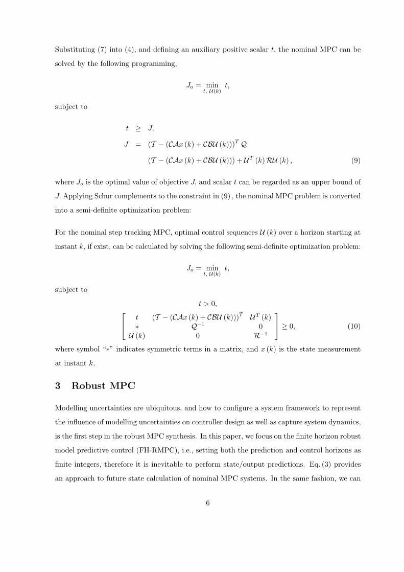
Substituting (7) into (4), and defining an auxiliary positive scalar t, the nominal MPC can be

solved by the following programming,

Jo = mint, U(k)

t,

subject to

t ≥ J,

J = (T − (CAx (k) + CBU (k)))T Q

(T − (CAx (k) + CBU (k))) + UT (k)RU (k) , (9)

where Jo is the optimal value of objective J, and scalar t can be regarded as an upper bound of

J. Applying Schur complements to the constraint in (9) , the nominal MPC problem is converted

into a semi-definite optimization problem:

For the nominal step tracking MPC, optimal control sequences U (k) over a horizon starting at

instant k, if exist, can be calculated by solving the following semi-definite optimization problem:

Jo = mint, U(k)

t,

subject to

t > 0,

t (T − (CAx (k) + CBU (k)))T UT (k)∗ Q−1 0

U (k) 0 R−1

≥ 0, (10)

where symbol “∗” indicates symmetric terms in a matrix, and x (k) is the state measurement

at instant k.

3 Robust MPC

Modelling uncertainties are ubiquitous, and how to configure a system framework to represent

the influence of modelling uncertainties on controller design as well as capture system dynamics,

is the first step in the robust MPC synthesis. In this paper, we focus on the finite horizon robust

model predictive control (FH-RMPC), i.e., setting both the prediction and control horizons as

finite integers, therefore it is inevitable to perform state/output predictions. Eq. (3) provides

an approach to future state calculation of nominal MPC systems. In the same fashion, we can

6

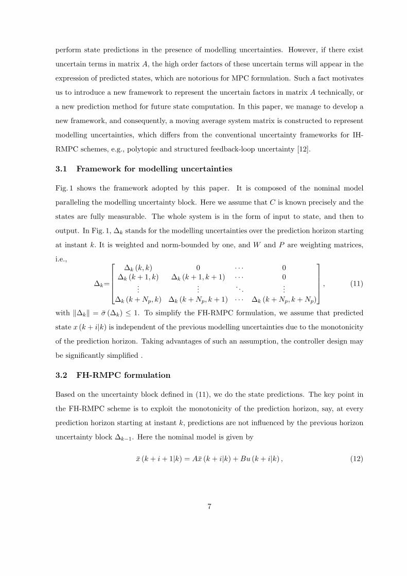
perform state predictions in the presence of modelling uncertainties. However, if there exist

uncertain terms in matrix A, the high order factors of these uncertain terms will appear in the

expression of predicted states, which are notorious for MPC formulation. Such a fact motivates

us to introduce a new framework to represent the uncertain factors in matrix A technically, or

a new prediction method for future state computation. In this paper, we manage to develop a

new framework, and consequently, a moving average system matrix is constructed to represent

modelling uncertainties, which differs from the conventional uncertainty frameworks for IH-

RMPC schemes, e.g., polytopic and structured feedback-loop uncertainty [12].

3.1 Framework for modelling uncertainties

Fig. 1 shows the framework adopted by this paper. It is composed of the nominal model

paralleling the modelling uncertainty block. Here we assume that C is known precisely and the

states are fully measurable. The whole system is in the form of input to state, and then to

output. In Fig. 1, ∆k stands for the modelling uncertainties over the prediction horizon starting

at instant k. It is weighted and norm-bounded by one, and W and P are weighting matrices,

i.e.,

∆k=

∆k (k, k) 0 · · · 0∆k (k + 1, k) ∆k (k + 1, k + 1) · · · 0

......

. . ....

∆k (k + Np, k) ∆k (k + Np, k + 1) · · · ∆k (k + Np, k + Np)

, (11)

with ‖∆k‖ = σ (∆k) ≤ 1. To simplify the FH-RMPC formulation, we assume that predicted

state x (k + i|k) is independent of the previous modelling uncertainties due to the monotonicity

of the prediction horizon. Taking advantages of such an assumption, the controller design may

be significantly simplified .

3.2 FH-RMPC formulation

Based on the uncertainty block defined in (11), we do the state predictions. The key point in

the FH-RMPC scheme is to exploit the monotonicity of the prediction horizon, say, at every

prediction horizon starting at instant k, predictions are not influenced by the previous horizon

uncertainty block ∆k−1. Here the nominal model is given by

x (k + i + 1|k) = Ax (k + i|k) + Bu (k + i|k) , (12)

7

and the uncertain term δ (k) caused by modelling uncertainties can be computed from

δ (k + i|k) =k+i∑

j=k

∆ (k + i, j) u (j|k) , (13)

where the uncertainty matrix ∆ is defined, for convenience, to be

∆ = P∆kW.

¿From (12) and (13), we have

x (k + i + 1|k) = x (k + i + 1|k) + δ (k + 1 + i|k)

= Ax (k + i|k) + Bu (k + i|k) +k+1+i∑

j=k

∆ (k + 1 + i, j) u (j|k) . (14)

It is obvious that

x (k + i|k) = x (k + i|k) + δ (k + i|k) = x (k + i|k) +k+i∑

j=k

∆ (k + i, j) u (j|k) . (15)

Substitute x (k + i|k) in (15) into (14), and derive

x (k + 1 + i|k) = Ax (k + i|k) + Bu (k + i|k) +k+1+i∑

j=k

∆ (k + 1 + i, j) u (j|k)

−Ak+i∑

j=k

∆ (k + i, j) u (j|k) . (16)

The predicted output satisfies

y (k + i|k) = Cx (k + i|k) . (17)

To illustrate the procedure of the state predictions, we implement the first two steps, i.e.,

calculations of x(k + 1|k) and x(k + 2|k),

x(k + 1|k) = Ax(k) + Bu(k|k) +k+1∑

j=k

∆(k + 1, j)u(j|k)−A∆(k, k)u(k|k), (18)

x(k + 2|k) = Ax(k + 1|k) + Bu(k + 1|k)

+k+2∑

j=k

∆(k + 2, j)u(j|k)−A

k+1∑

j=k

∆(k + 1, j)u(j|k). (19)

Substituting (18) into (19), we have

x(k + 2|k) = A2x(k) + ABu(k|k) + Bu(k + 1|k) +k+2∑

j=k

∆(k + 2, i)u(j|k) (20)

−A2∆(k, k)u(k|k).

8

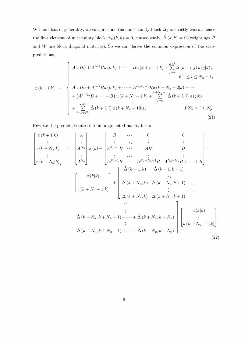
Without loss of generality, we can presume that uncertainty block ∆k is strictly causal, hence

the first element of uncertainty block ∆k (k, k) = 0, consequently, ∆ (k, k) = 0 (weightings P

and W are block diagonal matrices). So we can derive the common expression of the state

predictions,

x (k + i|k) =

Aix (k) + Ai−1Bu (k|k) + · · ·+ Bu (k + i− 1|k) +k+i∑j=k

∆ (k + i, j) u (j|k) ,

if 1 ≤ i ≤ Nu − 1,

Aix (k) + Ai−1Bu (k|k) + · · ·+ Ai−Nu+1Bu (k + Nu − 2|k) + · · ·+

(Ai−NuB + · · ·+ B

)u (k + Nu − 1|k) +

k+Nu−1∑j=k

∆ (k + i, j) u (j|k)

+k+i∑

j=k+Nu

∆ (k + i, j) u (k + Nu − 1|k) , if Nu ≤ i ≤ Np.

(21)

Rewrite the predicted states into an augmented matrix form:

x (k + 1|k)...

x (k + Nu|k)...

x (k + Np|k)

=

A...

ANu

...ANp

x (k) +

B · · · 0 0...

. . ....

...ANu−1B · · · AB B

... · · · ......

ANp−1B · · · ANp−Nu+1B ANp−NuB + · · ·+ B

·

u (k|k)...

u (k + Nu − 1|k)

+

∆ (k + 1, k) ∆ (k + 1, k + 1) · · ·...

. . ....

∆ (k + Nu, k) ∆ (k + Nu, k + 1) · · ·...

.... . .

∆ (k + Np, k) ∆ (k + Np, k + 1) · · ·0...

∆ (k + Nu, k + Nu − 1) + · · ·+ ∆ (k + Nu, k + Nu)...

∆ (k + Nu, k + Nu − 1) + · · ·+ ∆ (k + Np, k + Np)

u (k|k)...

u (k + Nu − 1|k)

.

(22)

9

Here we define two auxiliary matrices Ml and Mr as the left- and right-multipliers of uncertainty

block ∆, namely,

Ml =

0 I1 0 · · · 00 0 I1 · · · 0...

......

. . ....

0 0 0 · · · I1

, and Mr =

I2 0 0 0 00 I2 · · · 0 0...

.... . .

......

0 0 · · · I2 00 0 · · · 0 I2... · · · . . .

......

0 0 · · · 0 I2

, (23)

where both I1 ∈ Rn×n and I2 ∈ Rm×m are identity matrices. In terms of Ml and Mr, uncertainty

block ∆k defined in (11) can represent the uncertain terms in (22). Using the notation defined

in (5) and (8), we can rewrite (17) and (21) from i = 1 to i = Np in the augmented matrix

form as follows:

X (k) = Ax (k) + BU (k) + MlP∆kWMrU (k) ,

Y (k) = CX (k) , (24)

where X (k) is the augmented, predicted state vector,

X (k) =[

xT (k + 1|k) xT (k + 2|k) · · · xT (k + Np|k)]T

.

Motivated by the approach to nominal MPC, we now extend this approach to the case of

FH-RMPC:

A finite horizon robust MPC system can be represented by its corresponding nominal model in

parallel with a weighed unity-norm uncertainty block. Based on such a framework, robust step

tracking control, say, step tracking in the presence of modelling uncertainties, can be achieved

by solving a robust semi-definite optimization problem (if solutions exist) whose constraints

contain uncertain matrices:

Jo = mint, U(k)

t, (25)

subject to

t > 0,

max∆k

J ≤ t (with ‖∆k‖ = σ (∆k) ≤ 1) ,

J = (T − Y (k))T Q (T − Y (k)) + UT (k)RU (k) ,

X (k) = Ax (k) + BU (k) + MlP∆kWMrU (k) ,

Y (k) = CX (k) , (26)

10

where T is the augmented reference input, i.e.,

T =[

rT rT · · · rT]T

,

and t is an upper bound of the objective J.

¿From Eq. (25) , the objective J can be represented by

J = (T − (CAx (k) + CBU (k) + CMlP∆kWMrU (k)))T Q

(T − (CAx (k) + CBU (k)) + CMlP∆kWMrU (k)) + UT (k)RU (k) , (27)

and then in the same fashion as in the derivation in Eqs. (9) and (10) , condition (26) can be

created.

3.3 FH-RMPC algorithm based on LMIs

We have converted the FH-RMPC problem into the robust semi-definite optimization. Due to

the presence of modelling uncertainties, Eq. (26) comprises the uncertain terms of ∆k. There-

fore, we cannot apply Schur complements and use existing software packages to solve it numer-

ically. In order to overcome such a barrier, we first introduce the following Lemma:

Lemma 1 [16, 17] Let T1 = T T1 , and T2, T3, T4 be real matrices of appropriate sizes. Then

det (I − T4∆) 6= 0 and

T1 + T2∆(I − T4∆)−1 T3 + T T3 (I − T4∆)−T ∆T T T

2 ≥ 0 (28)

for every ∆, ‖∆‖ = σ (∆) ≤ 1, if and only if ‖T4‖ < 1 and there exists a scalar τ ≥ 0 such that[T1 − τT2T

T2 T T

3 − τT2TT4

T3 − τT4TT2 τ

(I − T4T

T4

)]≥ 0.

Proof. Here we assume T2 and T3 are non-zero (the result is straightforward if either of them

is zero). Pre- and post-multiplying zT and z to (28), we have

zT T1z + zT T2∆ (I − T4∆)−1 T3z + zT T T3 (I − T4∆)−T ∆T T T

2 z ≥ 0, (29)

where z is a non-zero vector with a proper dimension. Define by

ξ = (I − T4∆)−T ∆T T T2 z. (30)

11

Therefore (29) can be rewritten as[zξ

]T [T1 T T

3

T3 0

] [zξ

]≥ 0. (31)

Pre-multiplying both sides of (30) by (I − T4∆)T , we get

ξ = ∆T(T4ξ + T T

2 z).

Set p = T4ξ + T T2 z for simplicity, i.e., ξ = ∆T p. According to the condition ‖∆‖ = σ (∆) ≤ 1,

we can say

ξT ξ = pT ∆∆T p ≤ pT p.

Thus(T4ξ + T T

2 z)T (

T4ξ + T T2 z

)− ξT ξ ≥ 0,

i.e. [zξ

]T [T2T

T2 T2T

T4

T4TT2 T4T4 − I

] [zξ

]≥ 0. (32)

Using the S − procedure, we know that (32) is satisfied if and only if[T1 T T

3

T3 0

]− τ

[T2T

T2 T2T

T4

T4TT2 T4T4 − I

]≥ 0, (33)

where τ is a positive scalar. Rewrite (33) , and then Lemma 1 is proven. ¤

The key idea of the above Lemma is to employ an auxiliary positive scalar τ to convert

robust LMIs, namely, LMIs with some uncertain matrices, into standard LMI constraints.

Taking advantages of such a property, we can transform FH-RMPC for robust step tracking

control into a standard semi-definite optimization problem.

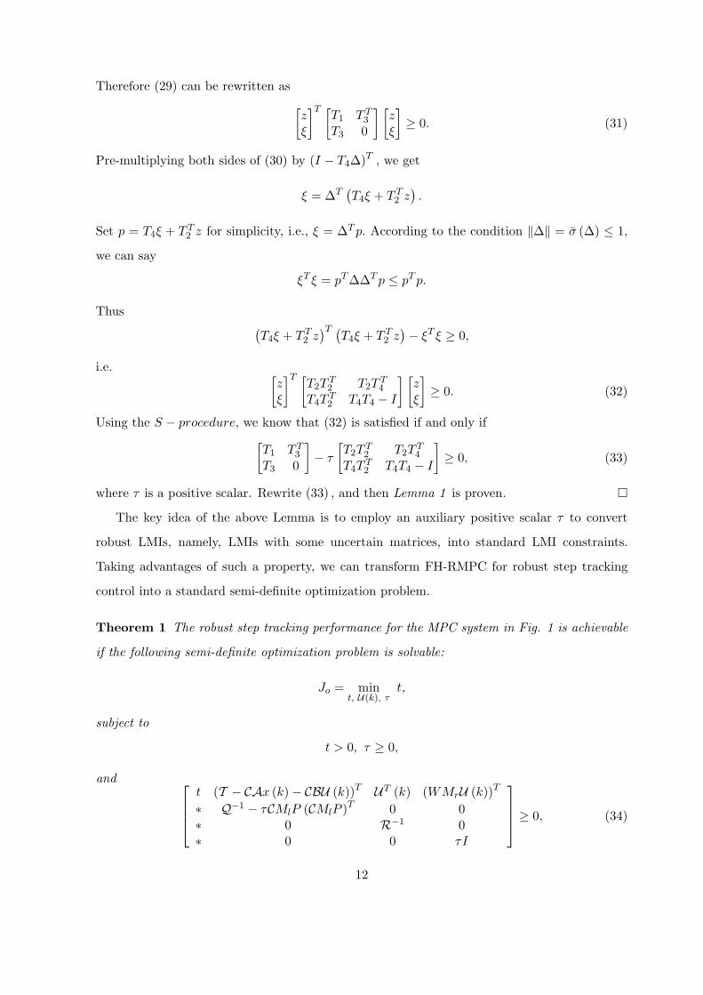
Theorem 1 The robust step tracking performance for the MPC system in Fig. 1 is achievable

if the following semi-definite optimization problem is solvable:

Jo = mint, U(k), τ

t,

subject to

t > 0, τ ≥ 0,

and

t (T − CAx (k)− CBU (k))T UT (k) (WMrU (k))T

∗ Q−1 − τCMlP (CMlP )T 0 0∗ 0 R−1 0∗ 0 0 τI

≥ 0, (34)

12

where I is an identity matrix. Augmented reference input T , predicted input sequence U (k) and

weighting matrices Q, R, are defined in (5) and (6) . The constant augmented matrices A, B,

C and left-, right- matrices Ml, Mr of uncertainty block ∆k in Fig. 1 are introduced in (8) and

(23).

Proof. Applying Schur complements and rewriting constraints in (26), we have

t (T − CAx (k)− CBU (k))T − (CMlP∆kWMrU (k))T UT (k)∗ Q−1 0

U (k) 0 R−1

≥ 0. (35)

Separating the certain and uncertain terms of (35),

T1 −

0 (CMlP∆kWMrU (k))T 00 0 00 0 0

−

0 0 0CMlP∆kWMrU (k) 0 0

0 0 0

≥ 0 (36)

and recasting (36), we have

T1 −

(WMrU (k))T

00

∆T

k

[0 (CMlP )T 0

]−

0CMlP

0

∆k

[WMrU (k) 0 0

] ≥ 0, (37)

where

T1 =

t (T − CAx (k)− CBU (k))T UT (k)∗ Q−1 0

U (k) 0 R−1

. (38)

Setting

T2 =

0−CMlP

0

, T3 =

[WMrU (k) 0 0

], and T4 = 0,

and putting (38) into the form of (28) , we can take advantages of the property described in

Lemma 1, i.e.,

T 1 − T T3 ∆T

k T T2 − T2∆kT3 ≥ 0 ⇔

[T1 − τT2T

T2 T T

3

T3 τI

]≥ 0. (39)

Therefore, it is not difficult to convert FH-RMPC for step tracking into a standard semi-definite

optimization problem. Theorem 1 is then proved. ¤

Theorem 1 provides an effective approach for solving FH-RMPC problems for robust step

tracking control. By adjusting the length of prediction horizon Np or/and control horizon Nu,

different requirements on the pre-specified performance may be satisfied. From the previous

theoretical analysis, if Np and Nu are large enough (for example Np = Nu = ∞) and optimal

13

control sequences do exist, we can find a Lyapunov function to guarantee closed-loop stability

of RMPC without any terminal constraints. However for the FH-RMPC case, the situation is

different. If both Np and Nu are finite, terminal cost constraints have to be imposed to facilitate

the robust stability analysis.

4 Terminal Cost Constraints

MPC strategies belong to feedback control areas. Although feedback helps to attenuate the

influence of modelling uncertainties, feedback can also lead to system instability. In 1988,

Keerthi and Gilbert first proposed a method which employed the objective function of MPC

systems as a Lyapunov function to solve the nominal stability problem [26]. Later the same

approach was used for nonlinear systems [27]. In this paper, we will employ a similar idea and

develop terminal cost constraints to guarantee robust stability of FH-RMPC systems.

4.1 LMIs for terminal cost constraints

Without loss of generality, here we set Np = Nu, otherwise we can enforce the terminal input

u (k + Nu − 1|k) = 0 to resume the following derivation. For ease of notation, we denote

e (k + i|k) , y (k + i|k)− r (k + i|k) . Consider a quadratic function

V (x (k + i|k)) = e (k + i|k)T Φe (k + i|k) = ‖Cx (k + i|k)− r‖2Φ , Φ > 0, (40)

of state measurement x (k) , k > 0. In the prediction horizon starting at instant k, we set

V (x (k + i + 1|k))− V (x (k + i|k)) < −(‖e (k + i|k)‖2

Q + ‖u (k + i|k)‖2R

), (41)

consequently,

V (x (k + Np|k))− V (x (k + Np − 1|k)) < −(‖e (k + Np − 1|k)‖2

Q + ‖u (k + Np − 1|k)‖2R

).

(42)

Summing Eqs. (41) and (42) from i = 0 to i = Np, we get

V (x (k + Np|k))− V (x (k|k)) < −J − ‖e (k)‖2Q + ‖e (k + Np|k)‖2

QNp.

In the sequel, we will employ V (x (k)) as a Lyapunov function satisfying

V (x (k)) > t + ‖e (k)‖2Q − ‖e (k + Np|k)‖2

QNp+ V (e (k + Np|k)) , (43)

14

where t is the upper bound of objective J defined in (26). Then V (k) : Rn → R, the difference

of Lyapunov functions of x (k + 1) and x (k) , can be defined as:

V (k) : = V (x (k + 1))− V (x (k))

< V (x (k + 1))− t− ‖e (k)‖2Q + ‖e (k + Np|k)‖2

Q′Np− V (x (k + Np|k)) . (44)

In order to derive closed-loop asymptotic stability, we should guarantee the right hand side of

(44) is negative, i.e.,

‖e (k + 1)‖2Φ − t− ‖e (k)‖2

Q + ‖e (k + Np|k)‖2QNp

− ‖e (k + Np|k)‖2Φ < 0. (45)

¿From (21) , we know that if u (k|k), the first element of input sequence U (k) is sent to the real

process, the state measurement at instant (k + 1) can be expressed as:

x (k + 1) = Ax (k) + Bu (k|k) + ∆ (k + 1, k) u (k|k) ,

consequently

e (k + 1) = CAx (k) + CBu (k|k) + C∆ (k + 1, k) u (k|k)− r. (46)

Introduce two constant matrices E1 and E2 such that

∆ (k + 1, k) = E1∆E2 = E1MlP∆kWMrE2, (47)

where

E1 =[0 I 0 · · · 0

], and E2 =

[I 0 · · · 0

]T.

Inserting (46) and (47) into (45) , we get

‖CAx (k) + CBu (k|k)− r + CE1MlP∆kWMrE2u (k|k)‖2Φ − t

−‖Cx (k)− r‖2Q + eT (k + Np|k)

(QNp − Φ

)e (k + Np|k) < 0 . (48)

So if the following two inequalities

‖Cx (k)− r‖2Q + t− ‖CAx (k) + CBu (k|k)− r + CE1MlP∆kWMrE2u (k|k)‖2

Φ > 0, (49)

Φ−QNp ≥ 0, (50)

hold simultaneously, we can guarantee the condition in (48). Applying Schur complements and

the property of robust LMIs (Lemma 1 ), we can recast (49) into:

‖Cx (k)− r‖2Q + t ∗ ∗

CAx (k) + CBu (k|k)− r X − λ1CE1MlP (CE1MlP )T ∗WMrE2u (k|k) 0 λ1I

> 0, (51)

15

where X = Φ−1 and λ1 is a positive scalar. Then left- and right-multiplying X to both sides of

inequality (50) and defining a small non-negative scale κ, which is selected as a tuning scalar

of(QNp + κI

), we have

X −X(QNp + κI

)X ≥ 0 (52)

It is obvious that if κ → 0, (52) is equivalent to (50) . Apply Schur complements to Eq. (52) and

derive [X X

X(QNp + κI

)−1

]≥ 0. (53)

Combined with (53) , (51) composes a sufficient condition to (45), which is designed for asymp-

totical stability of the closed-loop FH-RMPC system.

Meanwhile, in order to use V (x (k)) as a Lyapunov function candidate, in the sequel, we

will manage to derive another LMI to guarantee (43). To this end, taking advantages of the

condition in (50) , we can derive a sufficient condition to (43),

‖e (k)‖2QNp

− t− ‖e (k)‖2Q − ‖e (k + Np|k)‖2

Φ > 0. (54)

¿From (21) , x (k + Np|k) is expressed as:

e (k + Np|k) = CANpx (k) + CE3BU (k) + CE3MlP∆kWMrU (k)− r, (55)

where E3 =[0 · · · 0 0 I

], and I is an identity matrix with a proper dimension. Substituting

(55) into (54), applying Schur complements and using the property of robust LMIs, we get

‖Cx (k)− r‖2

QNp− ‖Cx (k)− r‖2

Q − t ∗ ∗CANpx (k) + CE3BU (k)− r X − λ2CE3MlP (CE3MlP )T ∗

WMrU (k) 0 λ2I

> 0, (56)

where λ2 is a positive scalar.

Theorem 2 To achieve step tracking performance for the FH-RMPC system defined in Fig.

1, manipulated input uo (k) = E4Uo (k|k) , k > 0, can be obtained by minimizing the following

optimization problem:

Jo = minU(k)

t,

16

subject to (34) , (51) , (53) and (56), where X, λ1 and λ2 are variables of LMIs for terminal

cost constraints, and E4 is a truncation matrix, given by

E4 =[I 0 · · · 0

].

The closed-loop system is guaranteed asymptotically stable if the optimal input sequences

Uo (k) =[

uo (k|k)T uo (k + 1|k)T · · · uo (k + Nu − 1|k)T]T

, k > 0,

do exist.

Proof. From Theorem 1 we know that the robust semi-definite optimization problem in Eq.

(26) , can be solved by minimizing the linear objective in Eq. (34) . Meanwhile, combined with

constraints (51) , (53) and (56) , the quadratic function of e (k) ,

V (x (k)) = eT (k)Φe (k) ,

can be regarded as a Lyapunov function, which is convergent with MPC iteration. Therefore,

by adding additional constraints (51) , (53) and (56) into the optimization problem defined in

(34) , we can guarantee the resulting FH-RMPC regulator is asymptotically stable, associated

with the Lyapunov function V (x (k)). ¤

5 Simulation Example

Consider a classical angular positioning system proposed by Kwakernaak and Sivan in 1972

[28]. The system model is written as:

[x1 (k + 1)x2 (k + 1)

]=

[1 0.10 1− 0.1α

]x (k) +

[0

0.787

]u (k) , (57)

y (k) =[1 0

]x (k) ,

where α ∈ [0.1, 10] reflects the uncertain coefficient of viscous friction in system’s physical

structure. Based on approaches discussed in [7], an IH-RMPC controller for the modelling

uncertainties in the form of the structured feedback loop, is first designed. Comparing with the

FH-RMPC controllers considered in this paper, it can be seen that the FH-RMPC controllers

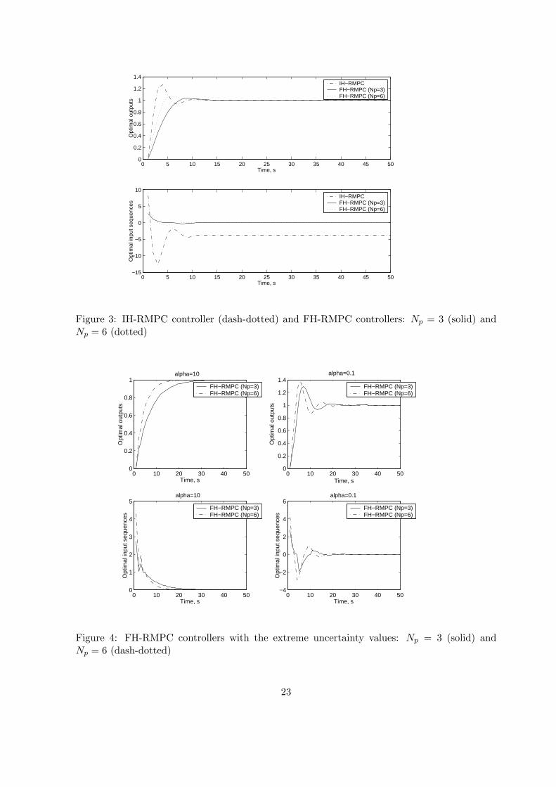
have the better tracking performance and smaller overshoot of the optimal input sequences (Fig.

3). Here the tuning parameters are selected as: r = 1, Q = I, QNp = I, R = 0.00002I, P =

17

I, Nu = 3 and W = 0.1. The simulation length equals to 50. For the simulation results

presented in Fig. 3, α = 0.7 (nominal value α = 0.495). In order to reconfigure the system

in (57) into the framework of Fig. 1, we can take advantages of the method described in Fig.

2, i.e., using the difference between the nominal model and real process to derive uncertainty

block ∆.

Let us increase and decrease uncertain term α oppositely till its left and right bounds,

i.e., setting α = 10 and α = 0.1, respectively. In the same fashion, we first design the IH-

RMPC controller. However, we find that it takes very long time to reach the steady-state value

and serious ripples occur and therefore was not presented. Fig. 4 shows the simulation results

based on FH-RMPC controllers with the different control horizons. FH-RMPC can achieve the

prespecified tracking even under extreme conditions. From this point, the FH-RMPC algorithm

proposed in this paper has a better robustness property. Similar to nominal MPC controllers,

FH-RMPC controllers also possess the property that if increasing the difference between Np

and Nu, the overshoot of performance decreases; meanwhile, system responses become slower.

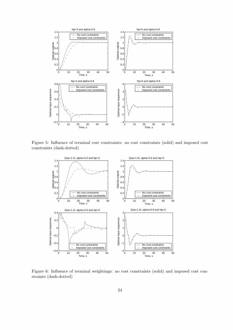
As discussed above, closed-loop stability is one of serious problems in FH-RMPC controller

design. By imposing several extra terminal cost constraints, we can guarantee that the resulting

system is closed-loop stable. Fig. 5 demonstrates the influence of the imposed terminal cost

constraints on the system performance with the different prediction horizons Np. Here we set

α = 0.8 and the control horizon Nu = 3. It can be seen that the terminal cost constraints

manage to attenuate the input and output peeks, meanwhile derive slower responses. Fig. 6

demonstrates the influence of the terminal cost constraints on the system performance with

the different terminal weightings QNp . We reset α = 0.9, Np = 3 and keep Nu = 3. In the

figures, solid lines (no cost constraints) are derived from Theorem 1, and dash-dotted lines from

Theorem 2. It can be seen that for some systems, even though we do not impose extra terminal

cost constraints, the FH-RMPC algorithm can still come to closed-loop stability.

All the simulations were performed on a PC with a Pentium 4 processor, 512MB RAM,

using the software LMI Control Toolbox [29] in the Matlab environment to compute solutions

of the linear minimization problem. Table 1 shows that the on-line computational cost can

be reduced by choosing FH-RMPC controllers. In the table, the numbers parenthesized are

average time to compute uo (k) over every prediction horizon, and the other is for the total

time with the simulation length equal to 50 (Np = Nu = 3).

18

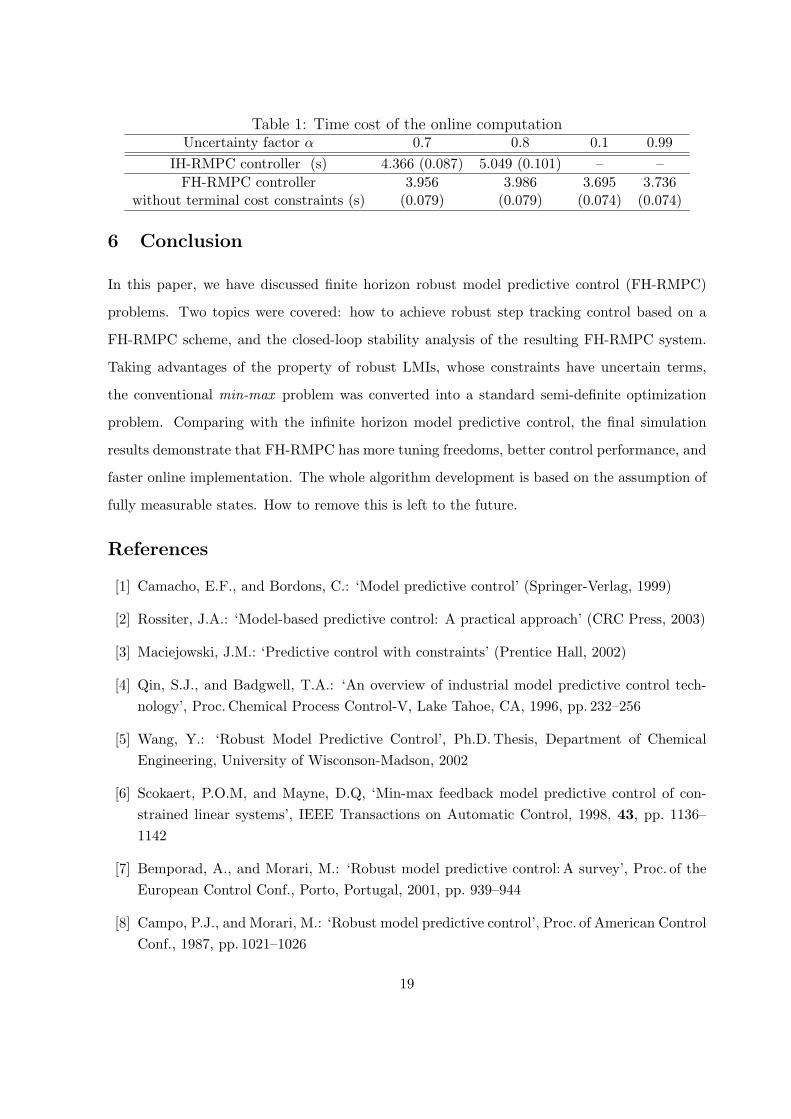
Table 1: Time cost of the online computationUncertainty factor α 0.7 0.8 0.1 0.99

IH-RMPC controller (s) 4.366 (0.087) 5.049 (0.101) – –FH-RMPC controller 3.956 3.986 3.695 3.736

without terminal cost constraints (s) (0.079) (0.079) (0.074) (0.074)

6 Conclusion

In this paper, we have discussed finite horizon robust model predictive control (FH-RMPC)

problems. Two topics were covered: how to achieve robust step tracking control based on a

FH-RMPC scheme, and the closed-loop stability analysis of the resulting FH-RMPC system.

Taking advantages of the property of robust LMIs, whose constraints have uncertain terms,

the conventional min-max problem was converted into a standard semi-definite optimization

problem. Comparing with the infinite horizon model predictive control, the final simulation

results demonstrate that FH-RMPC has more tuning freedoms, better control performance, and

faster online implementation. The whole algorithm development is based on the assumption of

fully measurable states. How to remove this is left to the future.

References

[1] Camacho, E.F., and Bordons, C.: ‘Model predictive control’ (Springer-Verlag, 1999)

[2] Rossiter, J.A.: ‘Model-based predictive control: A practical approach’ (CRC Press, 2003)

[3] Maciejowski, J.M.: ‘Predictive control with constraints’ (Prentice Hall, 2002)

[4] Qin, S.J., and Badgwell, T.A.: ‘An overview of industrial model predictive control tech-nology’, Proc. Chemical Process Control-V, Lake Tahoe, CA, 1996, pp. 232–256

[5] Wang, Y.: ‘Robust Model Predictive Control’, Ph.D. Thesis, Department of ChemicalEngineering, University of Wisconson-Madson, 2002

[6] Scokaert, P.O.M, and Mayne, D.Q, ‘Min-max feedback model predictive control of con-strained linear systems’, IEEE Transactions on Automatic Control, 1998, 43, pp. 1136–1142

[7] Bemporad, A., and Morari, M.: ‘Robust model predictive control: A survey’, Proc. of theEuropean Control Conf., Porto, Portugal, 2001, pp. 939–944

[8] Campo, P.J., and Morari, M.: ‘Robust model predictive control’, Proc. of American ControlConf., 1987, pp. 1021–1026

19

[9] Lee, J.H., and Yu, Z.: ‘Worst-case formulations of model predictive control for systemswith bounded parameters’, Automatica, 1997, 33, pp. 763–781

[10] Lee, J.H., and Cooley, B.L.: ‘Min-max predictive control techniques for a linear state-spacesystem with a bounded set of input matrices’, Automatica, 2000, 36, pp. 463–473

[11] Kothare, M.V., Balakrishnan, V., and Morari, M.: ‘Roust constrained model predictivecontrol using linear matrix inequalities’, Automatica, 1996, 32, pp. 1361–1379

[12] Boyd, S., Ghaoui, L.E., Feron, E., and Balakrishnan, V.: ‘Linear matrix inequalities incontrol theory’ (SIAM, Philadelphia, 1994)

[13] Vanderbei, R.J.: ‘Linear Programming: Foundations and Extensions’ (Kluwer AcademicPublishers, Boston Hardbound, 2001)

[14] Rodrigues, M.A., and Odloak, D.: ‘MPC for stable linear systems with model uncertainty’,Automatica, 2003, 39, pp. 569–583

[15] Wan, Z., and Kothare, M.V.: ‘An efficient off-line formulation of robust model predictivecontrol using linear matrix inequalities’, Automatica, 2003, 39, pp. 837–846

[16] Hu, B., and Linnemann, A.: ‘Toward infinite-horizon optimality in nonlinear model pre-dictive control’, IEEE Trans. on Autom.Control, 2002, 47, pp. 679–683

[17] Magni, L., Nicolao, G.D., Scattolini, R. and Allgower, F. ‘Robust model predictive controlof nonlinear discrete-time systems’, International Journal of Robust and Nonlinear Control,2003, 13, pp. 229–246

[18] Bemporad, A., Morari, M., and Ricker, N.L.: ‘MPC Control Toolbox for use with Matlab’(Mathworks, 2005)

[19] Mayne, D.Q., Rawlings, J.B., Rao, C.V., and Scokaert, P.: ‘Constrained model predictivecontrol: stability and optimality’, Automatica, 2000, 36, pp. 789–814

[20] Park, P. and Jeong, S.C.: ‘Constrained RHC for LPV systems with bounded rates ofparameter variations’, Automatica, 2004, 40, pp. 865–872

[21] Langson, W., Chryssochoos, I., Rakovic, S., and Mayne, D.Q.: ‘Robust model predictivecontrol using tubes’, Automatica, 2004, 40, pp. 125–133

[22] Fukushima, H. and Bitmead, R.R.: ‘Robust constrained predictive control using compari-son model’, Automatica, 2005, 41, pp. 97–106

[23] Chen, T. and Francis, B.: ‘Optimal sampled-data control systems’ (Springer, 1995)

[24] Ghaout, L.E., and Lebret, H.: ‘Robust solutions to least-squares problems with uncertaindata’, SIAM J.Matrix Anal. Appl., 1997, 18, pp. 1035-1064

20

[25] Lofberg, J.: ‘Minimax MPC for systems with uncertain input gain — revisited’, TechnicalReports, Automatic Control Group in Linkoping University, 2001

[26] Keerthi, S.S., and Gilbert, E.G.: ‘Optimal infinite horizon feedback laws for a general classof constrained discrete time systems: stability and moving-horizon approximations’, J. ofOptim.Theory and Appl., 1988, 57, pp. 265–293

[27] Mayne, D.Q., and Michalska, H.: ‘Receding horizon control of non-linear systems’, IEEETrans. on Autom. Control, 1990, 35, pp. 614–824

[28] Kwakernaak, H., and Sivan, R.: ‘Linear optimal control systems’ (Wiley-interscience, NewYork, 1972)

[29] Gahinet, P., Nemirovski, A., Lamb, A.J., and Chilali, M.: ‘LMI Control Toolbox for usewith Matlab’ (Mathworks, 1995)

21

0I

BA

W k P

CMPC controller

k

ku kxkrky+

kx

Figure 1: An FH-RMPC system

Real Process

P

Nominal Model

N

Nominal Model

N+

+

+

-

MPC Controller)(kx)(kx

)(k)(ku)(kr

ˆModeling Uncertainty Block

Figure 2: Modelling uncertainty reconfiguration

22

0 5 10 15 20 25 30 35 40 45 500

0.2

0.4

0.6

0.8

1

1.2

1.4

Time, s

Opt

imal

out

puts

0 5 10 15 20 25 30 35 40 45 50−15

−10

−5

0

5

10

Time, s

Opt

imal

inpu

t seq

uenc

es

IH−RMPCFH−RMPC (Np=3)FH−RMPC (Np=6)

IH−RMPCFH−RMPC (Np=3)FH−RMPC (Np=6)

Figure 3: IH-RMPC controller (dash-dotted) and FH-RMPC controllers: Np = 3 (solid) andNp = 6 (dotted)

0 10 20 30 40 500

0.2

0.4

0.6

0.8

1alpha=10

Time, s

Opt

imal

out

puts

0 10 20 30 40 500

1

2

3

4

5alpha=10

Time, s

Opt

imal

inpu

t seq

uenc

es

0 10 20 30 40 500

0.2

0.4

0.6

0.8

1

1.2

1.4alpha=0.1

Time, s

Opt

imal

out

puts

0 10 20 30 40 50−4

−2

0

2

4

6 alpha=0.1

Time, s

Opt

imal

inpu

t seq

uenc

es

FH−RMPC (Np=3)FH−RMPC (Np=6)

FH−RMPC (Np=3)FH−RMPC (Np=6)

FH−RMPC (Np=3)FH−RMPC (Np=6)

FH−RMPC (Np=3)FH−RMPC (Np=6)

Figure 4: FH-RMPC controllers with the extreme uncertainty values: Np = 3 (solid) andNp = 6 (dash-dotted)

23

0 10 20 30 40 500

0.2

0.4

0.6

0.8

1

1.2

1.4 Np=3 and alpha=0.8

Time, s

Opt

imal

out

puts

0 10 20 30 40 50−4

−2

0

2

4

6

Time, s

Opt

imal

inpu

t seq

uenc

es

Np=6 and alpha=0.8

0 10 20 30 40 50−0.2

0

0.2

0.4

0.6

0.8

Time, s

Opt

imal

inpu

t seq

uenc

es

Np=3 and alpha=0.8

0 10 20 30 40 500

0.2

0.4

0.6

0.8

1

1.2

1.4

Time, s

Opt

imal

out

puts

Np=6 and alpha=0.8

No cost constraintsImposed cost constraints

No cost constraintsImposed cost constraints

No cost constraintsImposed cost constraints

No cost constraintsImposed cost constraints

Figure 5: Influence of terminal cost constraints: no cost constraints (solid) and imposed costconstraints (dash-dotted)

0 10 20 30 40 500

0.2

0.4

0.6

0.8

1

1.2

1.4Qnp=1.2I, alpha=0.9 and Np=3

Time, s

Opt

imal

out

puts

0 10 20 30 40 50−2

−1

0

1

2

3

Time, s

Opt

imal

inpu

t seq

uenc

es

Qnp=1.5I, alpha=0.9 and Np=3

0 10 20 30 40 50−0.6

−0.4

−0.2

0

0.2

0.4

Time, s

Opt

imal

inpu

t seq

uenc

es

Qnp=1.2I, alpha=0.9 and Np=3

0 10 20 30 40 500

0.2

0.4

0.6

0.8

1

1.2

1.4

Time, s

Opt

imal

out

puts

Qnp=1.5I, alpha=0.9 and Np=3

No cost constraints Imposed cost constraints

No cost constraints Imposed cost constraints

No cost constraints Imposed cost constraints

No cost constraints Imposed cost constraints

Figure 6: Influence of terminal weightings: no cost constraints (solid) and imposed cost con-straints (dash-dotted)

24