Nonlinear Output-Feedback Model Predictive Control with

Moving Horizon Estimation: Illustrative Examples

David A. Copp and João P. Hespanha˚

October 28, 2015

Abstract

We review a recently introduced method to efficiently solve online optimization problems that appearin output-feedback model predictive control (MPC) and moving-horizon state estimation (MHE). Thenovel feature of this approach is that it solves both the MPC and MHE problems simultaneously as asingle min-max optimization. Like in the more common state-feedback MPC, this approach allows one toincorporate explicit constraints on the control input and state. In addition, it allows one to incorporateany known constraints on disturbances and noise.

Under appropriate assumptions that ensure controllability and observability of the nonlinear processto be controlled, we give results showing that the state of the system remains bounded and establishbounds on the tracking error for trajectory tracking problems.

The min-max optimization that arises in our approach can be solved using a primal-dual-like interior-point method, developed especially for this purpose. Under appropriate convexity assumptions, thismethod is guaranteed to terminate at a global solution. However, simulation results show that it alsoconverges rapidly in many problems that are severely nonconvex.

This report includes a few representative examples that demonstrate the applicability of the approachin systems that are high-dimensional, nonlinear in their dynamics and/or measurements, and that havesignificant dynamic uncertainty. For all these examples, the interior-point method solver takes on averageless than 6 ms to compute the control signal on a regular laptop computer.

1 Introduction

Advances in computer technology have made online optimization a viable and powerful tool for solvingcontrol problems in practical applications. Model predictive control (MPC) is an approach that uses onlineoptimization to solve an open-loop optimal control problem at each sampling time and is now quite matureas evidenced by [1–4]. In MPC, the current state of the plant to be controlled is used as an initial conditionfrom which an online optimization is solved. This optimization yields an optimal control sequence from whichthe first control action in the sequence is selected and applied to the plant. Then, at each sampling timethis technique is repeated. A useful tutorial overview of MPC is given in [5].

MPC is often attractive in many applications because it can explicitly handle hard state and inputconstraints, but a downside to MPC is the computational complexity involved in solving these problems

˚D. A. Copp and J. P. Hespanha are with the Center for Control, Dynamical Systems, and Computation, University of California,Santa Barbara, CA 93106 USA. dacopp@engr.ucsb.edu,hespanha@ece.ucsb.edu

1

rapidly online. Because MPC problems require the solution of an optimization problem at each samplingtime, efficient numerical methods for solving these problems are imperative for effective control. In the past,MPC has been popular in many industries where plant dynamics are slow enough to accommodate the timenecessary to numerically compute solutions online. Now that computational efficiency has increased, MPCis penetrating even more areas in industry. For a survey of MPC applications in industry, see [6].

Other important considerations when implementing an MPC controller include robustness to model pa-rameter uncertainty, additive input disturbances, and measurement noise. The study of these topics areknown as robust, worst-case, or min-max MPC. Initial results on these topics are discussed in works such as[7–10]. In order to alleviate problems from uncertainties, noise, and disturbances, MPC is often formulatedassuming full-state feedback. In practical cases, however, the full state often cannot be measured and is notavailable for feedback. This motivates the investigation of robust output-feedback MPC in which the use of anindependent algorithm for state estimation is required. Examples of algorithms for state estimation includeobservers, filters, and moving horizon estimation, some of which are discussed in [11]. Of these methods,moving horizon estimation (MHE) is attractive for use with MPC because it explicitly handles constraintsand computes the optimal current estimate of the state by solving an online optimization problem over afixed number of past measurements. Therefore, the computational cost does not grow as more measurementsbecome available. Nonlinear MPC and MHE are are both discussed in [12]. A useful overview of constrainednonlinear moving horizon state estimation is given in [13], and more recent results regarding stability of MHEcan be found in [14].

Thus far, results on the stability of output-feedback control schemes based on MPC and MHE (especiallyfor nonlinear systems) are limited. In this report, we consider the output-feedback of nonlinear systems withuncertainty and disturbances, and formulate the MPC problem as a min-max optimization as introduced in[15, 16]. In this formulation, a desired cost function is maximized over disturbance and noise variables andminimized over control input variables. In this way, we can solve both the MPC and MHE problems usinga single min-max optimization, which gives us an optimal control input sequence at each sampling time fora worst-case estimate of the current state. For finite-horizon optimizations, we show that the state remainsbounded under the proposed feedback control law. We also show that the tracking error in trajectory trackingproblems is bounded in the presence of measurement noise and input disturbances.

The main assumption for our results is that a saddle-point solution exists for the min-max optimizationat each sampling time. This assumption is a common requirement in game theoretical approaches to controldesign [17] and presumes appropriate forms of observability and controllability of the closed-loop system. Weadditionally require the minor assumptions that the dynamics are reversible and that there exists a terminalcost that is an ISS-control Lyapunov function with respect to a disturbance input.

Several algorithms are available to numerically solve the class of min-max optimization problems that wediscuss here. A few methods are discussed in [18] and [19] and include sequential quadratic programming,interior-point methods, and others. We use a primal-dual-like interior-point algorithm as described in [16]to solve this min-max optimization. Under appropriate convexity assumptions, this method is guaranteedto terminate at a global solution. However, simulation results show that it also converges rapidly in manyproblems that are severely nonconvex. This report includes a few representative examples that demonstratethe applicability of the approach in systems that are high-dimensional, nonlinear in their dynamics and/ormeasurements, and that have significant dynamic uncertainty.

The paper is organized as follows. First, we briefly describe related work that has been done in theareas of model predictive control, moving horizon estimation, numerical methods for min-max optimizationproblems, and specifically primal-dual methods. In Section 2, we formulate the control problem we would liketo solve and discuss its relationship to MPC and MHE. In Section 3, we state the main closed-loop stability

2

results. Simulation results are presented in Section 5, and we provide some conclusions and directions forfuture research in Section 6.

Related Work

Model predictive control, moving horizon estimation, and numerical optimization are each large areas ofstudy, so now we mention some related work to narrow our focus. As discussed in the introduction, thestudy of model predictive control is quite mature as evidenced by [1–4]. Robust and worst-case MPC isinitially discussed in works such as [7–10]. Min-max MPC for constrained linear systems is considered in [20]and [21], and a game theoretic approach for robust constrained nonlinear MPC is proposed in [22]. Recentstudies of input-to-state stability of min-max MPC can be found in [23–25], however these references do notinvestigate the use of output-feedback. Nominal or inherent robustness of MPC has also been studied in[3, 26].

Because MPC and MHE problems can be formulated as similar optimization problems, and becauseoutput-feedback MPC requires some form of state estimation, during the same time that many importantresults on MPC were developed, parallel work was being done on MHE. Nice overviews of constrained linearand nonlinear moving horizon state estimation can be found in [13, 27, 28]. Recent results regarding stabilityof MHE can be found in [14]. Nonlinear MPC and MHE are both discussed in [12]. Some joint stabilityresults for state estimation and control are given in [29], but again, output-feedback MPC is not considered.Recently, more work has been done on output-feedback MPC. A survey including some nonlinear results isgiven in [30]. Results on robust output-feedback MPC for constrained linear systems can be found in [31]using a state observer for estimation, and in [32] using MHE for estimation. Fewer results are available fornonlinear output-feedback MPC, although notable exceptions are [3, 33].

There is extensive literature involving the derivation of methods to numerically solve optimization prob-lems, such as those that appear in MPC and MHE, efficiently and reliably. A good resource for studyingconvex optimization problems and methods to solve them (including interior-point and primal-dual interior-point methods) is the book [34]. Work regarding interior-point methods can be found in [35, 36] and primal-dualinterior-point methods in particular in [37]. The application of interior-point algorithms as a method to solveMPC problems is discussed in [38]. Other early work on efficient numerical methods for solving MPC problemsare given in [39], [40], and [37]. Advances in computational efficiency have allowed for the fast solution ofMPC problems using online optimization such as in the more recent work [41]. The real-time solution ofthe MHE problem for small dimensional nonlinear models is given in [18]. Considering specifically numericalmethods for min-max MPC optimization problems, the authors in [42] set up and solve min-max MPC asa quadratic program. Robust dynamic programming for min-max MPC of constrained uncertain systems isconsidered in [43], while sequential quadratic programming and interior-point methods for solving nonlinearMPC with MHE problems are discussed in [19]. The particular primal-dual-like interior-point method thatwe implement is inspired by the primal-dual interior-point method for a single optimization given in [44].

2 Problem Formulation

As in [15] and [16], we consider the control of a time-varying nonlinear discrete-time process of the form

xt`1 “ ftpxt , ut , dtq, yt “ gtpxtq ` nt , @t P Zě0 (1)

with state xt taking values in a set X Ă Rnx . The inputs to this system are the control input ut that must be

restricted to the set U Ă Rnu , the unmeasured disturbance dt that is known to belong to the set D Ă R

nd ,

3

Controller

Sensor

System

Disturbance(d)

Noise(n)

SystemOutput

MeasuredOutput(y)

ReferenceMeasurederror

Control(u)+

-

++

+

+

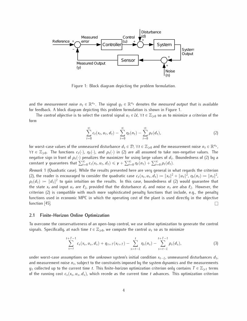
Figure 1: Block diagram depicting the problem formulation.

and the measurement noise nt P Rnn . The signal yt P R

ny denotes the measured output that is availablefor feedback. A block diagram depicting this problem formulation is shown in Figure 1.

The control objective is to select the control signal ut P U, @t P Zě0 so as to minimize a criterion of theform

8ÿ

t“0

ctpxt , ut , dtq ´8ÿ

t“0

ηtpntq ´8ÿ

t“0

ρtpdtq, (2)

for worst-case values of the unmeasured disturbance dt P D , @t P Zě0 and the measurement noise nt P Rnn ,

@t P Zě0. The functions ctp¨q, ηtp¨q, and ρtp¨q in (2) are all assumed to take non-negative values. Thenegative sign in front of ρtp¨q penalizes the maximizer for using large values of dt . Boundedness of (2) by aconstant γ guarantees that

ř8t“0 ctpxt , ut , dtq ď γ `

ř8t“0 ηtpntq `

ř8t“0 ρtpdtq.

Remark 1 (Quadratic case). While the results presented here are very general in what regards the criterion(2), the reader is encouraged to consider the quadratic case ctpxt , ut , dtq – }xt}

2 ` }ut}2, ηtpntq – }nt}

2,ρtpdtq – }dt}

2 to gain intuition on the results. In this case, boundedness of (2) would guarantee thatthe state xt and input ut are ℓ2, provided that the disturbance dt and noise nt are also ℓ2. However, thecriterion (2) is compatible with much more sophisticated penalty functions that include, e.g., the penaltyfunctions used in economic MPC in which the operating cost of the plant is used directly in the objectivefunction [45]. l

2.1 Finite-Horizon Online Optimization

To overcome the conservativeness of an open-loop control, we use online optimization to generate the controlsignals. Specifically, at each time t P Zě0, we compute the control ut so as to minimize

t`T ´1ÿ

s“t

cspxs, us, dsq ` qt`T pxt`T q ´t

ÿ

s“t´L

ηspnsq ´t`T ´1

ÿ

s“t´L

ρspdsq, (3)

under worst-case assumptions on the unknown system’s initial condition xt´L, unmeasured disturbances dt ,and measurement noise nt , subject to the constraints imposed by the system dynamics and the measurementsyt collected up to the current time t . This finite-horizon optimization criterion only contains T P Zě1 termsof the running cost cspxs, us, dsq, which recede as the current time t advances. This optimization criterion

4

also only contains L ` 1 P Zě1 terms of the measurement cost ηspnsq. The function qt`T pxt`T q acts as aterminal cost in order to penalize the “final” state at time t ` T .

Since the goal is to optimize this cost at the current time t to compute the control inputs at times s ě t ,there is no point in penalizing the running cost cspxs, us, dsq for past time instants s ă t , which explainsthe fact that the first summation in (3) starts at time t . There is also no point in considering the valuesof future measurement noise at times s ą t , as they will not affect choices made at time t , which explainsthe fact that the second summation in (3) stops at time t . However, we do need to consider all values forthe unmeasured disturbance ds, because past values affect the (unknown) current state xt and future valuesaffect the future values of the running cost.

At a given time t P Zě0, we do not know the value of the variables xt´L and dt´L:t`T ´11 on which

the value of the criterion (3) depends, so we optimize for the future controls ut:t`T ´1 under worst-caseassumptions on xt´L and dt´L:t`T ´1, leading to the following min-max optimization

J˚t “ min

ut:t`T ´1PUmax

xt´LPX ,dt´L:t`T ´1PD

t`T ´1ÿ

s“t

cspxs, us, dsq ` qt`T pxt`T q

´t

ÿ

s“t´L

ηs

`

ys ´ gspxsq˘

´t`T ´1

ÿ

s“t´L

ρspdsq, (4)

with the understanding that

xs`1 “

#

fspxs, us, dsq for t ´ L ď s ă t,

fspxs, us, dsq for t ď s ă t ` T .

We can view the optimization variables xt´L and dt´L:t`T ´1 as (worst-case) estimates of the initial stateand disturbances, respectively, based on the past inputs ut´L:t´1 and outputs yt´L:t available at time t .

Inspired by model predictive control, at each time t , we use as the control input the first element of thesequence

u˚t:t`T ´1 “ tu˚

t , u˚t`1, u˚

t`2, . . . , u˚t`T ´1u P U

that minimizes (4), leading to the following control law:

ut “ u˚t , @t ě 0. (5)

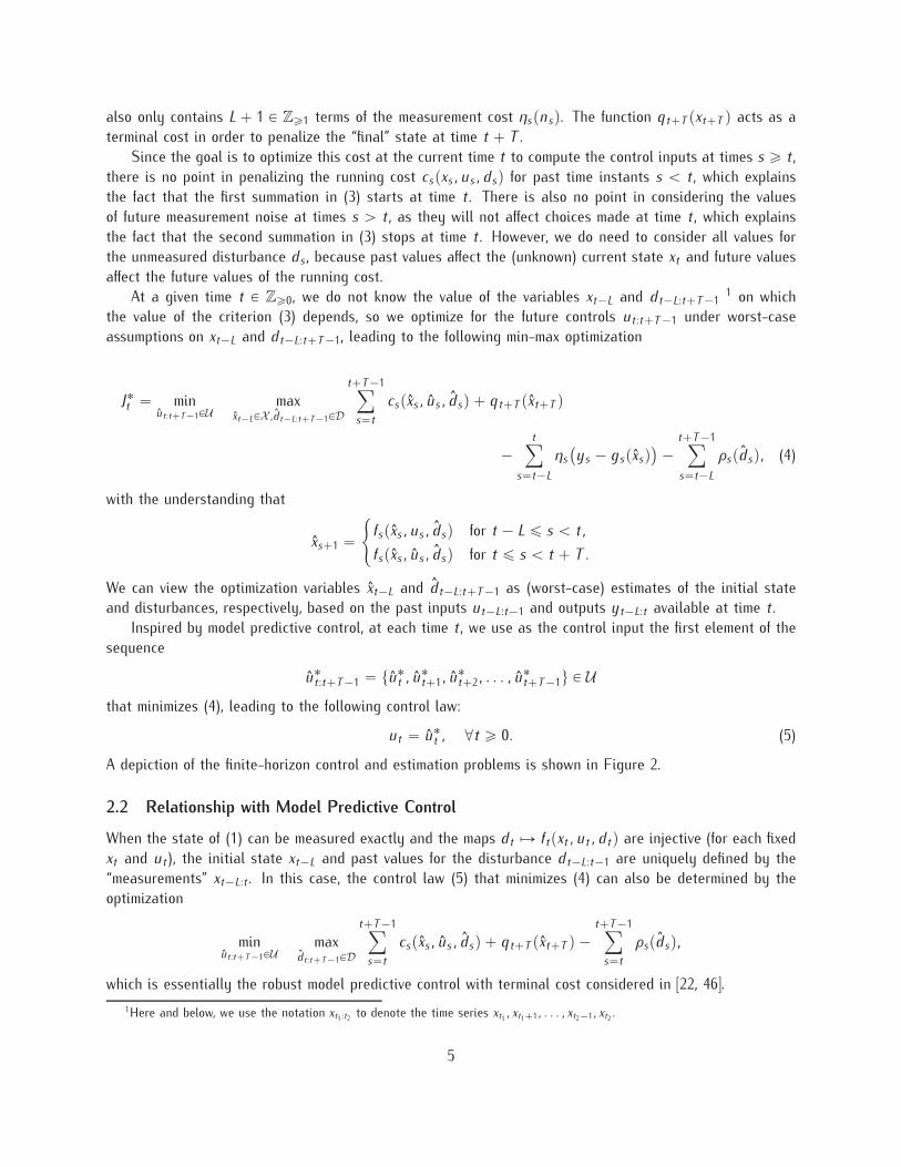
A depiction of the finite-horizon control and estimation problems is shown in Figure 2.

2.2 Relationship with Model Predictive Control

When the state of (1) can be measured exactly and the maps dt ÞÑ ftpxt , ut , dtq are injective (for each fixedxt and ut ), the initial state xt´L and past values for the disturbance dt´L:t´1 are uniquely defined by the“measurements” xt´L:t . In this case, the control law (5) that minimizes (4) can also be determined by theoptimization

minut:t`T ´1PU

maxdt:t`T ´1PD

t`T ´1ÿ

s“t

cspxs, us, dsq ` qt`T pxt`T q ´t`T ´1

ÿ

s“t

ρspdsq,

which is essentially the robust model predictive control with terminal cost considered in [22, 46].

1Here and below, we use the notation xt1 :t2 to denote the time series xt1 , xt1`1, . . . , xt2´1, xt2 .

5

t+Ttt-L

y(t-L)

y(t) x*(t+T)

u0:t-L-1 ut-L:t-1

d0:t-L-1 d*t-L:t-1

u*t:t+T-1

d*t:t+T-1

Figure 2: Finite-horizon control and estimation problems. The elements in blue correspond to the MHEproblem, and the elements in red correspond to the MPC problem.

2.3 Relationship with Moving-Horizon Estimation

When setting both csp¨q and qt`T p¨q equal to zero in the criterion (4), this optimization no longer dependson ut:t`T ´1 and dt:t`T ´1, so the optimization in (4) simply becomes

maxxt´LPX ,dt´L:t´1PD

´t

ÿ

s“t´L

ηs

`

ys ´ gspxsq˘

´t´1ÿ

s“t´L

ρspdsq,

where now the optimization criterion only contains a finite number of terms that recedes as the current timet advances, which is essentially the moving horizon estimation problem considered in [13, 14].

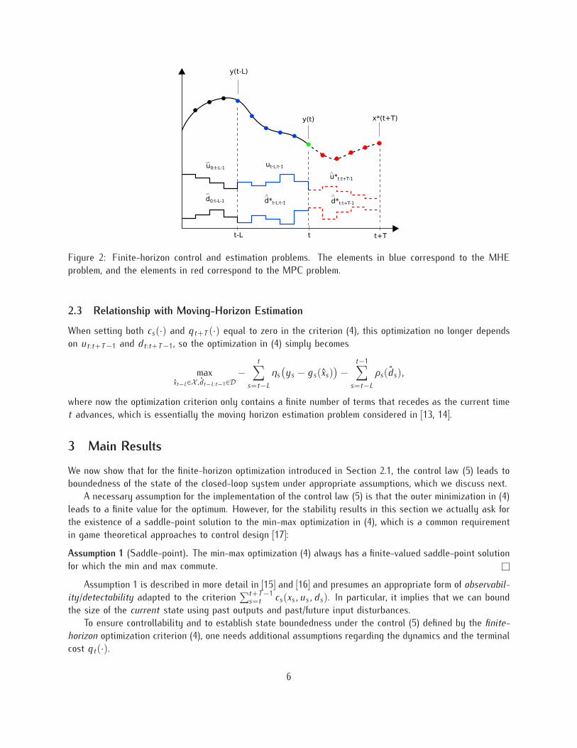
3 Main Results

We now show that for the finite-horizon optimization introduced in Section 2.1, the control law (5) leads toboundedness of the state of the closed-loop system under appropriate assumptions, which we discuss next.

A necessary assumption for the implementation of the control law (5) is that the outer minimization in (4)leads to a finite value for the optimum. However, for the stability results in this section we actually ask forthe existence of a saddle-point solution to the min-max optimization in (4), which is a common requirementin game theoretical approaches to control design [17]:

Assumption 1 (Saddle-point). The min-max optimization (4) always has a finite-valued saddle-point solutionfor which the min and max commute. l

Assumption 1 is described in more detail in [15] and [16] and presumes an appropriate form of observabil-

ity/detectability adapted to the criterionřt`T ´1

s“t cspxs, us, dsq. In particular, it implies that we can boundthe size of the current state using past outputs and past/future input disturbances.

To ensure controllability and to establish state boundedness under the control (5) defined by the finite-

horizon optimization criterion (4), one needs additional assumptions regarding the dynamics and the terminalcost qtp¨q.

6

Assumption 2 (Reversible Dynamics). For every t P Zě0, xt`1 P X , and ut P U, there exists a state xt P X

and a disturbance dt P D such that

xt`1 “ ftpxt , ut , dtq. (6)

l

Assumption 3 (ISS-control Lyapunov function). The terminal cost qtp¨q is an ISS-control Lyapunov function,in the sense that, for every t P Zě0, x P X , there exists a control u P U such that

qt`1

`

ftpx, u, dq˘

´ qtpxq ď ´ctpx, u, dq ` ρtpdq, @d P D . (7)

l

Assumption 2 is very mild and essentially means that the sets of disturbances D and past states X aresufficiently rich to allow for a jump to any future state in X . Assumption 3 plays the role of a commonassumption in model predictive control, namely that the terminal cost must be a control Lyapunov functionfor the closed-loop [47]. In the absence of the disturbance dt , (7) would mean that qtp¨q could be viewedas a control Lyapunov function that decreases along system trajectories for an appropriate control input ut

[48]. With disturbances, qtp¨q needs to be viewed as an ISS-control Lyapunov function that satisfies an ISSstability condition for the disturbance input dt and an appropriate control input ut [49].

Remark 2. When the dynamics are linear, for instance, Assumption 2 is satisfied if the state-space A matrixhas no eigenvalues at the origin (e.g., if it results from the time-discretization of a continuous-time system).When, the dynamics are linear and the cost function is quadratic, a terminal cost qtp¨q satisfying Assumption 3is typically found by solving a system of linear matrix inequalities. l

3.1 Finite-Horizon Online Optimization

The following theorem is the main result of this section and provides a bound that can be used to proveboundedness of the state when the control signal is constructed using the finite-horizon criterion (3). Thisresult first appeared in [15], and its proof can be found in [16].

Theorem 1 (Finite-horizon cost-to-go bound). Suppose that Assumptions 1, 2, and 3 hold. Then there exists

a finite constant J˚0 and vectors ds P R

nd , ns P Rnn , @s P t0, 1, . . . , t ´ L ´ 1u for which

ηspnsq, ρspdsq ă 8, @s P t0, 1, t ´ L ´ 1u,

and the trajectories of the process (1) with control (5) defined by the finite-horizon optimization (4) satisfy

ctpxt , ut , dtq ď J˚0 `

t´L´1ÿ

s“0

ηspnsq `t´L´1

ÿ

s“0

ρspdsq `t

ÿ

s“t´L

ηspnsq `t

ÿ

s“t´L

ρspdsq, @t P Zě0 (8)

l

The termsřt´L´1

s“0 ηspnsq `řt´L´1

s“0 ρspdsq in the right-hand side of (8) can be thought of as the arrival

cost that appears in the MHE literature to capture the quality of the estimate at the beginning of the currentestimation window [13]. In what follows, for simplicity of presentation we no longer distinguish between ds

and ds or ns and ns, but instead simply write ds and ns.Next we discuss the implications of Theorem 1 in terms of establishing bounds on the state of the

closed-loop system, asymptotic stability, and the ability of the closed-loop to asymptotically track desiredtrajectories.

7

3.1.1 State boundedness and asymptotic stability

When we select criterion (3) for which there exists a class2 K8 function αp¨q and class K functions βp¨q, δp¨qsuch that

ctpx, u, dq ě αp}x}q, ηtpnq ď βp}n}q, ρtpdq ď δp}d}q, @x P Rnx , u P R

nu , d P Rnd , n P R

nn ,

we conclude from (8) that, along trajectories of the closed-loop system, we have

αp}xt}q ď J˚0 `

tÿ

s“0

βp}ns}q `t

ÿ

s“0

δp}ds}q, @t P Zě0. (9)

This provides a bound on the state provided that the noise and disturbances are “vanishing,” in the sensethat

8ÿ

s“0

βp}ns}q ă 8,

8ÿ

s“0

δp}ds}q ă 8.

Theorem 1 can also provide bounds on the state for non-vanishing noise and disturbances, when we useexponentially time-weighted functions ctp¨q, ηtp¨q, and ρtp¨q that satisfy

ctpx, u, dq ě λ´tαp}x}q, ηtpnq ď λ´tβp}n}q, ρtpdq ď λ´tδp}d}q, @x P Rnx , u P R

nu , d P Rnd , n P R

nn ,

(10)

for some λ P p0, 1q, in which case we conclude from (8) that

αp}xt}q ď λtJ˚0 `

tÿ

s“0

λt´sβp}ns}q `t

ÿ

s“0

λt´sδp}ds}q, @t P Zě0.

Therefore, xt remains bounded provided that the measurement noise nt and the unmeasured disturbance dt

are both uniformly bounded. Moreover, }xt} converges to zero as t Ñ 8, when the noise and disturbancesvanish asymptotically. We have proved the following:

Corollary 1. Suppose that Assumption 1 holds and also that (10) holds for a class K8 function αp¨q, class K

functions βp¨q, δp¨q, and λ P p0, 1q. Then, for every uniformly bounded measurement noise sequence n0:8, and

uniformly bounded disturbance sequence d0:8, the state xt remains uniformly bounded along the trajectories

of the process (1) with control (5) defined by the finite-horizon optimization (4). Moreover, when dt and nt

converge to zero as t Ñ 8, the state xt also converges to zero. l

Remark 3 (Time-weighted criteria). The exponentially time-weighted functions (10) typically arise from cri-terion of the form

t`T ´1ÿ

s“t

λ´scpxs, us, dsq ´t

ÿ

s“t´L

λ´sηpnsq ´t`T ´1

ÿ

s“t´L

λ´sρpdsq

that weight the future more than the past. In this case, (10) holds for functions α , β , and δ such thatcpx, u, dq ě αp}x}q, ηpnq ď βp}n}q, and ρpdq ď δp}d}q, @x, u, d, n. l

2A function α : Rě0 Ñ Rě0 is said to belong to class K if it is continuous, zero at zero, and strictly increasing; and to belongto class K8 if it belongs to class K and is unbounded.

8

3.1.2 Reference tracking

When the control objective is for the state xt to follow a given trajectory zt , the optimization criterion canbe selected of the form

t`T ´1ÿ

s“t

λ´scpxs ´ zs, us, dsq ´t

ÿ

s“t´L

λ´sηpnsq ´t`T ´1

ÿ

s“t´L

λ´sρpdsq.

with cpx, u, dq ě αp}x}q, @x, u, d for some class K8 function α and λ P p0, 1q. In this case, we concludefrom (8) that

αp}xt ´ zt}q ď λtJ˚0 `

tÿ

s“0

λt´sηpnsq `t

ÿ

s“0

λt´sρpdsq, @t P Zě0,

which allows us to conclude that xt converges to zt as t Ñ 8, when both nt and dt are vanishing sequences,and also that, when these sequences are “ultimately small”, the tracking error xt ´ zt will converge to asmall value.

4 Computation of Control by Solving a Pair of Coupled Optimizations

To implement the control law (5) we need to find the control sequence u˚t:t`T ´1 P U that achieves the

outer minimizations in (4). In view of Assumption 1, the desired control sequence must be part of a saddle-point. From the perspective of numerically computing this saddle point, it is convenient to use the followingcharacterization of the saddle point:

´J˚t “ min

pdt´L:t`T ´1,xt´L:t`T qPD rut´L:t´1,u˚

t:t`T ´1s´

t`T ´1ÿ

s“t

cspxs, u˚s , dsq ´ qt`T pxt`T q

`t

ÿ

s“t´L

ηs

`

ys ´ gspxsq˘

`t`T ´1

ÿ

s“t´L

ρspdsq (11a)

J˚t “ min

put´L:t`T ´1,xt´L:t`T qPUrx˚

t´L,d˚

t´L:t`T ´1s

t`T ´1ÿ

s“t

cspxs, us, d˚s q ` qt`T pxt`T q

´t

ÿ

s“t´L

ηs

`

ys ´ gspxsq˘

´t`T ´1

ÿ

s“t´L

ρspd˚s q (11b)

where

D rut´L:t´1, u˚t:t`T ´1s –

!

pdt´L:t`T ´1|t, xt´L:t`T q :dt´L:t`T ´1 P D , xt´L:t`T P X ,

xs`1 “ fspxs, us, dsq, @s P tt ´ L, ..., t ´ 1u,

xs`1 “ fspxs, u˚s , dsq, @s P tt, ..., t ` T ´ 1u

)

, (12a)

Urx˚t´L, d˚

t´L:t`T ´1s –

!

put:t`T ´1, xt´L`1:t`T q :ut:t`T ´1 P U, xt´L`1:t`T P X ,

xt´L`1 “ fspx˚t´L, ut´L, d˚

t´Lq,

9

xs`1 “ fspxs, us, d˚s q, @s P tt ´ L ` 1, ..., t ´ 1u,

xs`1 “ fspxs, us, d˚s q, @s P tt, ..., t ` T ´ 1u

)

. (12b)

Essentially, we introduced the values of the state from time t-L+1 to time t ` T as additional optimizationvariables that are constrained by the system dynamics.

Using this characterization of the saddle point, we have developed a primal-dual-like interior-pointmethod to find it, inspired by the primal-dual interior-point method for a single optimization given in [44].We do not discuss this method here, but details of the method can be found in [16]. Under appropriateconvexity assumptions, this method is guaranteed to terminate at a global solution. However, simulationresults show that it also converges rapidly in many problems that are severely nonconvex.

5 Validation through Simulation

In this section we consider several examples and present closed-loop simulations using the control approachintroduced in Section 2. For all of the following examples, we use a cost function of the form

t`T ´1ÿ

s“t

}hspxsq}22 ` λu

t`T ´1ÿ

s“t

}us}22 ´ λn

tÿ

s“t´L

}ns}22 ´ λd

t`T ´1ÿ

s“t´L

}ds}22. (13)

where hspxsq is a function of the state xs that is especially relevant for the example under consideration,and λu, λn, and λd are positive weighting constants.

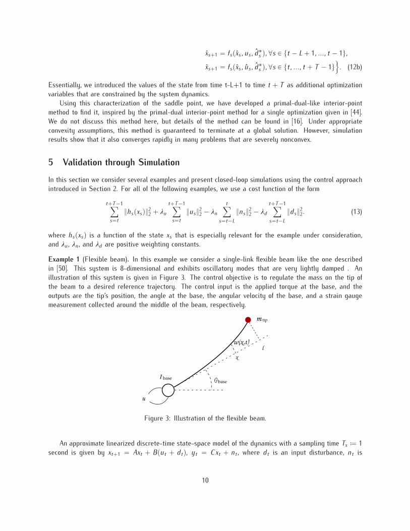
Example 1 (Flexible beam). In this example we consider a single-link flexible beam like the one describedin [50]. This system is 8-dimensional and exhibits oscillatory modes that are very lightly damped . Anillustration of this system is given in Figure 3. The control objective is to regulate the mass on the tip ofthe beam to a desired reference trajectory. The control input is the applied torque at the base, and theoutputs are the tip’s position, the angle at the base, the angular velocity of the base, and a strain gaugemeasurement collected around the middle of the beam, respectively.

I

u

l

x

m

w(x,t)

base

tip

base

Figure 3: Illustration of the flexible beam.

An approximate linearized discrete-time state-space model of the dynamics with a sampling time Ts – 1second is given by xt`1 “ Axt ` Bput ` dtq, yt “ Cxt ` nt , where dt is an input disturbance, nt is

10

measurement noise, and the system matrices are given by

A “

»

—

—

—

—

—

–

1.0 1.016 ´0.676 ´1.084 1.0 0.585 0.233 0.0320 ´0.665 1.241 1.783 0 0.042 ´0.288 ´0.0230 0.009 ´0.439 0.143 0 ´0.002 ´0.012 0.0070 0.001 0.014 0.308 0 ´0.000 0.001 0.0010 1.264 ´37.070 10.581 1.0 1.016 ´0.676 ´1.0840 ´2.109 59.920 ´16.883 0 ´0.665 1.241 1.7830 0.413 9.156 ´3.695 0 0.009 ´0.439 0.1430 ´0.012 ´0.371 ´3.929 0 0.001 0.014 0.308

fi

ffi

ffi

ffi

ffi

ffi

fl

,

B “ r0.800 ´0.797 0.003 0.001 1.327 ´1.163 0.197 ´0.006s1 ,

C “

»

–

1.13 0.7225 ´0.2028 0.1220 0 0 0 01.0 0 0 0 0 0 0 00 0 0 0 1.0 0 0 00 0.9282 ´12.001 ´35.294 0 0 0 0

fi

fl . (14)

This matrix A has a double eigenvalue at 1 with a single independent eigenvector. Therefore this is anunstable system.

The optimal control input is found by solving the optimization (4) with the cost function given in (13), withhspxsq “ ps ´ rs , where ps is the position of the mass at the tip of the beam and rs is a desired referencetrajectory, U – tut P R

nu : ´umax ď ut ď umaxu, X – R8, and D – tdt P R

nd : ´dmax ď dt ď dmaxu.The results depicted in Figure 4 show the response of the closed loop system under the control law (5)

when our goal is to regulate the mass at the tip of the beam to a desired reference rt – α sgnpsinpωtqqwith α “ 0.5 and ω “ 0.1. The other parameters in the optimization have values λu “ 1, λd “ 2, λn “ 100,L “ 5, T “ 5, umax “ 0.8, dmax “ 0.8. The state of the system starts close to zero and evolves withzero control input and small random disturbance input until time t “ 6, at which time the optimal controlinput (5) started to be applied along with the optimal worst-case disturbance d˚

t obtained from the min-maxoptimization. The noise process nt was selected to be a zero-mean Gaussian independent and identicallydistributed random process with a standard deviation of 0.01. l

0 10 20 30 40 50 60 70 80−0.8

−0.6

−0.4

−0.2

0

0.2

0.4

0.6

0.8

u˚

d˚

y

t

r

Figure 4: Simulation results of Flexible Beam example. The reference is in red, the measured output in blue,the control sequence in green, and the disturbance sequence in magenta.

Example 2 (Riderless bicycle). In this example we consider an unstable linear system with impulsive additiveinput disturbances. It corresponds to the riderless bicycle described in [51], where the control objective is to

11

0 5 10 15 20 25

Rol

l and

Ste

er A

ngle

s [d

eg]

-40

-30

-20

-10

0

10

20

30

40

Roll Angle [deg]Steer Angle [deg]

t

(a) Results of riderless bicycle example. The steer angle is inblue, and the roll angle is in red.

0 5 10 15 20 25

Ste

erin

g to

rque

and

dis

turb

ance

s [N

m]

-1

-0.8

-0.6

-0.4

-0.2

0

0.2

0.4

0.6

0.8

1

u*d

t

(b) Value of control inputs u˚ (in green) from min-max opti-mization and impulsive disturbances d (in magenta).

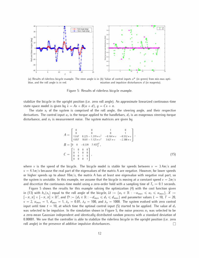
Figure 5: Results of riderless bicycle example.

stabilize the bicycle in the upright position (i.e. zero roll angle). An approximate linearized continuous-timestate-space model is given by 9x “ Ax ` Bpu ` dq, y “ Cx ` n.

The state xt of the system is comprised of the roll angle, the steering angle, and their respectivederivatives. The control input ut is the torque applied to the handlebars, dt is an exogenous steering-torquedisturbance, and nt is measurement noise. The system matrices are given by

A “

»

–

0 0 1 00 0 0 1

13.67 0.225 ´ 1.319 ˚ v2 ´0.164 ˚ v ´0.552 ˚ v

4.857 10.81 ´ 1.125 ˚ v2 3.621 ˚ v ´2.388 ˚ v

fi

fl ,

B “ r0 0 ´0.339 7.457s1 ,

C “

»

–

1 0 0 00 1 0 00 0 1 00 0 0 1

fi

fl , (15)

where v is the speed of the bicycle. The bicycle model is stable for speeds between v “ 3.4m{s andv “ 4.1m{s because the real part of the eigenvalues of the matrix A are negative. However, for lower speedsor higher speeds up to about 10m{s, the matrix A has at least one eigenvalue with negative real part, sothe system is unstable. In this example, we assume that the bicycle is moving at a constant speed v “ 2m{s

and discretize the continuous-time model using a zero-order hold with a sampling time of Ts – 0.1 seconds.Figure 5 shows the results for this example solving the optimization (4) with the cost function given

in (13) with hspxsq equal to the roll angle of the bicycle, U :“ tut P R : ´umax ď ut ď umaxu, X :“r´π, πs ˆ r´π, πs ˆ R

2, and D :“ tdt P R : ´dmax ď dt ď dmaxu and parameter values L “ 10, T “ 20,v “ 2, umax “ 1, dmax “ 1, λu “ 0.01, λd “ 100, and λn “ 1000. The system evolved with zero controlinput until time t “ 10, at which time the optimal control input (5) started to be applied. The value of dt

was selected to be impulsive. In the simulation shown in Figure 5, the noise process nt was selected to bea zero-mean Gaussian independent and identically distributed random process with a standard deviation of0.00001. We see that the controller is able to stabilize the riderless bicycle in the upright position (i.e. zeroroll angle) in the presence of additive impulsive disturbances. l

12

0 10 20 30 40 50 60 70 80 90 100-25

-20

-15

-10

-5

0

5

10

15

u*yref

t

(a) Results of model uncertainty example. The measured out-put is in blue, the control sequence in green, and the referencesignal in red.

0 10 20 30 40 50 60 70 80 90 100-0.8

-0.6

-0.4

-0.2

0

0.2

0.4

0.6

0 10 20 30 40 50 60 70 80 90 1000.2

0.3

0.4

0.5

0.6

0.7

0.8

ac

t

t

(b) Value of a and c from min-max optimization.

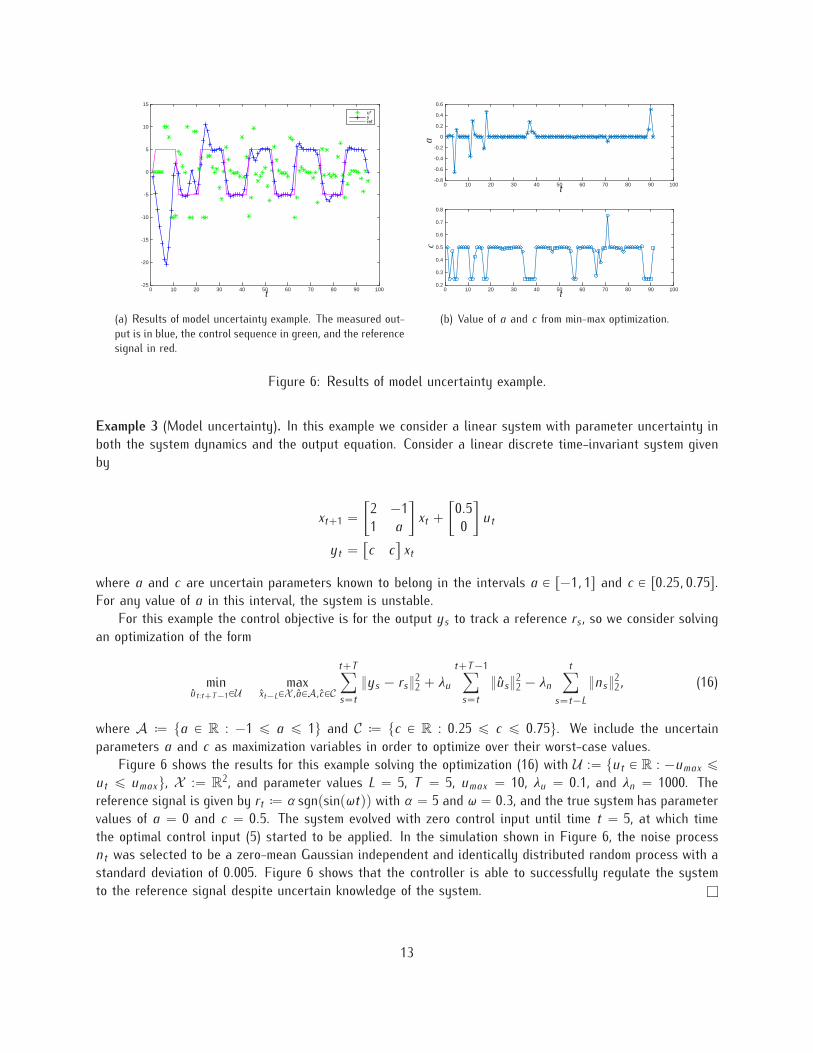
Figure 6: Results of model uncertainty example.

Example 3 (Model uncertainty). In this example we consider a linear system with parameter uncertainty inboth the system dynamics and the output equation. Consider a linear discrete time-invariant system givenby

xt`1 “

„

2 ´11 a

xt `

„

0.50

ut

yt ““

c c‰

xt

where a and c are uncertain parameters known to belong in the intervals a P r´1, 1s and c P r0.25, 0.75s.For any value of a in this interval, the system is unstable.

For this example the control objective is for the output ys to track a reference rs, so we consider solvingan optimization of the form

minut:t`T ´1PU

maxxt´LPX ,aPA,cPC

t`Tÿ

s“t

}ys ´ rs}22 ` λu

t`T ´1ÿ

s“t

}us}22 ´ λn

tÿ

s“t´L

}ns}22, (16)

where A – ta P R : ´1 ď a ď 1u and C – tc P R : 0.25 ď c ď 0.75u. We include the uncertainparameters a and c as maximization variables in order to optimize over their worst-case values.

Figure 6 shows the results for this example solving the optimization (16) with U :“ tut P R : ´umax ďut ď umaxu, X :“ R

2, and parameter values L “ 5, T “ 5, umax “ 10, λu “ 0.1, and λn “ 1000. Thereference signal is given by rt – α sgnpsinpωtqq with α “ 5 and ω “ 0.3, and the true system has parametervalues of a “ 0 and c “ 0.5. The system evolved with zero control input until time t “ 5, at which timethe optimal control input (5) started to be applied. In the simulation shown in Figure 6, the noise processnt was selected to be a zero-mean Gaussian independent and identically distributed random process with astandard deviation of 0.005. Figure 6 shows that the controller is able to successfully regulate the systemto the reference signal despite uncertain knowledge of the system. l

13

Example 4 (Nonlinear pursuit-evasion). In this example we investigate a two-player pursuit-evasion gamewhere the pursuer is modeled as a nonholonomic unicycle-type vehicle, and the evader is modeled as adouble-integrator. The following equations are used to model this example

x1t`1 “ x1t ` v cospθtq,

x2t`1 “ x2t ` v sinpθtq,

θt`1 “ θt ` ut ,

z1t`1 “ z1t ` d1t ,

z2t`1 “ z2t ` d2t ,

where v is a constant scalar corresponding to the velocity of the pursuer, xt ““

x1t x2t

‰1P R

2 is theposition of the pursuer at time t , θt P r0, 2πs is the orientation of the pursuer at time t , ut P R is the control

input at time t , zt ““

z1t z2t

‰1P R

2 is the position of the evader at time t , and dt ““

d1t d2t

‰1P R

2

is the evader’s “acceleration" at time t . We assume that the control input ut is bounded by the positiveconstant umax , and “acceleration" of the evader dt is bounded by the positive constant dmax . The output ofthe system is given by yt “

“

xt zt

‰1`

“

n1t n2t

‰1, where nt “

“

n1t n2t

‰1P R

2 is measurement noise.The pursuer’s goal is to make the distance between its position xt and the position of the evader zt as

small as possible, so the pursuer wants to minimize the value of }zt ´ xt}. The evader’s goal is to do theopposite, namely, maximize the value of }zt ´ xt}. The pursuer and evader try to achieve these goals bychoosing appropriate values for ut and dt , respectively.

−0.5 0 0.5 1 1.5 2 2.5 3 3.5−1

−0.5

0

0.5

1

1.5

2

x1, z1

x 2,z

2

Unicycle-pursuerDouble integrator-evader

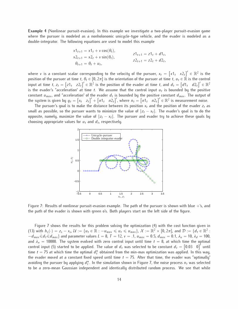
Figure 7: Results of nonlinear pursuit-evasion example. The path of the pursuer is shown with blue `’s, andthe path of the evader is shown with green o’s. Both players start on the left side of the figure.

Figure 7 shows the results for this problem solving the optimization (4) with the cost function given in(13) with hsp¨q “ zs ´ xs, U :“ tut P R : ´umax ď ut ď umaxu, X :“ R

2 ˆ r0, 2πs, and D :“ tdt P R2 :

´dmax 9ďdt 9ďdmaxu and parameter values L “ 8, T “ 12, v “ .1, umax “ 0.5, dmax “ 0.1, λu “ 10, λd “ 100,and λn “ 10000. The system evolved with zero control input until time t “ 8, at which time the optimalcontrol input (5) started to be applied. The value of dt was selected to be constant dt “

“

0.03 0‰1

untiltime t “ 75 at which time the optimal d˚

t obtained from the min-max optimization was applied. In this way,the evader moved at a constant fixed speed until time t “ 75. After that time, the evader was ”optimally"avoiding the pursuer by applying d˚

t . In the simulation shown in Figure 7, the noise process nt was selectedto be a zero-mean Gaussian independent and identically distributed random process. We see that while

14

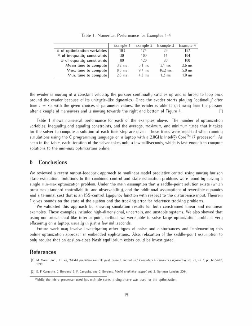
Table 1: Numerical Performance for Examples 1-4

Example 1 Example 2 Example 3 Example 4# of optimization variables 103 174 29 157# of inequality constraints 30 100 14 104

# of equality constraints 80 120 20 100Mean time to compute 3.2 ms 5.1 ms 3.1 ms 2.6 msMax. time to compute 8.3 ms 9.7 ms 16.2 ms 5.0 msMin. time to compute 2.8 ms 4.3 ms 1.2 ms 1.9 ms

the evader is moving at a constant velocity, the pursuer continually catches up and is forced to loop backaround the evader because of its unicycle-like dynamics. Once the evader starts playing “optimally" aftertime t “ 75, with the given choices of parameter values, the evader is able to get away from the pursuerafter a couple of maneuvers and is moving towards the right and bottom of Figure 4. l

Table 1 shows numerical performance for each of the examples above. The number of optimizationvariables, inequality and equality constraints, and the average, maximum, and minimum times that it takesfor the solver to compute a solution at each time step are given. These times were reported when runningsimulations using the C programming language on a laptop with a 2.8GHz Intel R© CoreTM i7 processor3. Asseen in the table, each iteration of the solver takes only a few milliseconds, which is fast enough to computesolutions to the min-max optimization online.

6 Conclusions

We reviewed a recent output-feedback approach to nonlinear model predictive control using moving horizonstate estimation. Solutions to the combined control and state estimation problems were found by solving asingle min-max optimization problem. Under the main assumption that a saddle-point solution exists (whichpresumes standard controllability and observability), and the additional assumptions of reversible dynamicsand a terminal cost that is an ISS-control Lyapunov function with respect to the disturbance input, Theorem1 gives bounds on the state of the system and the tracking error for reference tracking problems.

We validated this approach by showing simulation results for both constrained linear and nonlinearexamples. These examples included high-dimensional, uncertain, and unstable systems. We also showed thatusing our primal-dual-like interior-point method, we were able to solve large optimization problems veryefficiently on a laptop, usually in just a few milliseconds.

Future work may involve investigating other types of noise and disturbances and implementing thisonline optimization approach in embedded applications. Also, relaxation of the saddle-point assumption toonly require that an epsilon-close Nash equilibrium exists could be investigated.

References

[1] M. Morari and J. H Lee, “Model predictive control: past, present and future,” Computers & Chemical Engineering, vol. 23, no. 4, pp. 667–682,1999.

[2] E. F. Camacho, C. Bordons, E. F. Camacho, and C. Bordons, Model predictive control, vol. 2. Springer London, 2004.

3While the micro-processor used has multiple cores, a single core was used for the optimization.

15

[3] J. B. Rawlings and D. Q. Mayne, Model Predictive Control: Theory and Design. Nob Hill Publishing, 2009.

[4] L. Grüne and J. Pannek, Nonlinear Model Predictive Control. Springer, 2011.

[5] J. B. Rawlings, “Tutorial overview of model predictive control,” Control Systems, IEEE, vol. 20, no. 3, pp. 38–52, 2000.

[6] S. J. Qin and T. A. Badgwell, “A survey of industrial model predictive control technology,” Control engineering practice, vol. 11, no. 7, pp. 733–764,2003.

[7] P. J. Campo and M. Morari, “Robust model predictive control,” in American Control Conference, 1987, pp. 1021–1026, IEEE, 1987.

[8] J. a. Lee and Z. Yu, “Worst-case formulations of model predictive control for systems with bounded parameters,” Automatica, vol. 33, no. 5,pp. 763–781, 1997.

[9] A. Bemporad and M. Morari, “Robust model predictive control: A survey,” in Robustness in identification and control, pp. 207–226, Springer,1999.

[10] L. Magni, G. De Nicolao, R. Scattolini, and F. Allgöwer, “Robust model predictive control for nonlinear discrete-time systems,” InternationalJournal of Robust and Nonlinear Control, vol. 13, no. 3-4, pp. 229–246, 2003.

[11] J. B. Rawlings and B. R. Bakshi, “Particle filtering and moving horizon estimation,” Computers & chemical engineering, vol. 30, no. 10, pp. 1529–1541, 2006.

[12] F. Allgöwer, T. A. Badgwell, J. S. Qin, J. B. Rawlings, and S. J. Wright, “Nonlinear predictive control and moving horizon estimation-an introductoryoverview,” in Advances in control, pp. 391–449, Springer, 1999.

[13] C. V. Rao, J. B. Rawlings, and D. Q. Mayne, “Constrained state estimation for nonlinear discrete-time systems: Stability and moving horizonapproximations,” Automatic Control, IEEE Transactions on, vol. 48, no. 2, pp. 246–258, 2003.

[14] A. Alessandri, M. Baglietto, and G. Battistelli, “Moving-horizon state estimation for nonlinear discrete-time systems: New stability results andapproximation schemes,” Automatica, vol. 44, no. 7, pp. 1753–1765, 2008.

[15] D. A. Copp and J. P. Hespanha, “Nonlinear output-feedback model predictive control with moving horizon estimation,” in 53rd IEEE Conferenceon Decision and Control, pp. 3511–3517, IEEE, 2014.

[16] D. A. Copp and J. P. Hespanha, “Nonlinear output-feedback model predictive control with moving horizon estimation: Technical report,” tech.rep., Univ. California, Santa Barbara, 2014.

[17] T. Başar and G. J. Olsder, Dynamic Noncooperative Game Theory. London: Academic Press, 1995.

[18] M. J. Tenny and J. B. Rawlings, “Efficient moving horizon estimation and nonlinear model predictive control,” in American Control Conference,2002. Proceedings of the 2002, vol. 6, pp. 4475–4480, IEEE, 2002.

[19] M. Diehl, H. J. Ferreau, and N. Haverbeke, “Efficient numerical methods for nonlinear MPC and moving horizon estimation,” in Nonlinear ModelPredictive Control, pp. 391–417, Springer, 2009.

[20] P. Scokaert and D. Mayne, “Min-max feedback model predictive control for constrained linear systems,” Automatic Control, IEEE Transactionson, vol. 43, no. 8, pp. 1136–1142, 1998.

[21] A. Bemporad, F. Borrelli, and M. Morari, “Min-max control of constrained uncertain discrete-time linear systems,” Automatic Control, IEEETransactions on, vol. 48, no. 9, pp. 1600–1606, 2003.

[22] H. Chen, C. Scherer, and F. Allgöwer, “A game theoretic approach to nonlinear robust receding horizon control of constrained systems,” inAmerican Control Conference, 1997. Proceedings of the 1997, vol. 5, pp. 3073–3077, IEEE, 1997.

[23] M. Lazar, D. Muñoz de la Peña, W. Heemels, and T. Alamo, “On input-to-state stability of min–max nonlinear model predictive control,” Systems& Control Letters, vol. 57, no. 1, pp. 39–48, 2008.

[24] D. Limon, T. Alamo, D. Raimondo, D. M. de la Pena, J. Bravo, A. Ferramosca, and E. Camacho, “Input-to-state stability: a unifying framework forrobust model predictive control,” in Nonlinear model predictive control, pp. 1–26, Springer, 2009.

[25] D. M. Raimondo, D. Limon, M. Lazar, L. Magni, and E. Camacho, “Min-max model predictive control of nonlinear systems: A unifying overviewon stability,” European Journal of Control, vol. 15, no. 1, pp. 5–21, 2009.

[26] G. Grimm, M. J. Messina, S. E. Tuna, and A. R. Teel, “Nominally robust model predictive control with state constraints,” Automatic Control, IEEETransactions on, vol. 52, no. 10, pp. 1856–1870, 2007.

16

[27] C. V. Rao and J. B. Rawlings, “Nonlinear moving horizon state estimation,” in Nonlinear model predictive control, pp. 45–69, Springer, 2000.

[28] C. V. Rao, J. B. Rawlings, and J. H. Lee, “Constrained linear state estimation-a moving horizon approach,” Automatica, vol. 37, no. 10, pp. 1619–1628, 2001.

[29] J. Löfberg, “Towards joint state estimation and control in minimax MPC,” in Proceedings of 15th IFAC World Congress, Barcelona, Spain, 2002.

[30] R. Findeisen, L. Imsland, F. Allgöwer, and B. A. Foss, “State and output feedback nonlinear model predictive control: An overview,” Europeanjournal of control, vol. 9, no. 2, pp. 190–206, 2003.

[31] D. Q. Mayne, S. Raković, R. Findeisen, and F. Allgöwer, “Robust output feedback model predictive control of constrained linear systems: Timevarying case,” Automatica, vol. 45, no. 9, pp. 2082–2087, 2009.

[32] D. Sui, L. Feng, and M. Hovd, “Robust output feedback model predictive control for linear systems via moving horizon estimation,” in AmericanControl Conference, 2008, pp. 453–458, IEEE, 2008.

[33] L. Imsland, R. Findeisen, E. Bullinger, F. Allgöwer, and B. A. Foss, “A note on stability, robustness and performance of output feedback nonlinearmodel predictive control,” Journal of Process Control, vol. 13, no. 7, pp. 633–644, 2003.

[34] S. P. Boyd and L. Vandenberghe, Convex optimization. Cambridge university press, 2004.

[35] M. H. Wright, “The interior-point revolution in constrained optimization,” in High Performance Algorithms and Software in Nonlinear Optimization,pp. 359–381, Springer, 1998.

[36] A. Forsgren, P. E. Gill, and M. H. Wright, “Interior methods for nonlinear optimization,” SIAM review, vol. 44, no. 4, pp. 525–597, 2002.

[37] S. J. Wright, “Applying new optimization algorithms to model predictive control,” in AIChE Symposium Series, vol. 93, pp. 147–155, Citeseer,1997.

[38] C. V. Rao, S. J. Wright, and J. B. Rawlings, “Application of interior-point methods to model predictive control,” Journal of optimization theoryand applications, vol. 99, no. 3, pp. 723–757, 1998.

[39] L. Biegler and J. Rawlings, “Optimization approaches to nonlinear model predictive control,” tech. rep., Argonne National Lab., IL (USA), 1991.

[40] L. T. Biegler, “Efficient solution of dynamic optimization and NMPC problems,” in Nonlinear model predictive control, pp. 219–243, Springer,2000.

[41] Y. Wang and S. Boyd, “Fast model predictive control using online optimization,” Control Systems Technology, IEEE Transactions on, vol. 18,no. 2, pp. 267–278, 2010.

[42] D. M. de la Pena, T. Alamo, D. Ramirez, and E. Camacho, “Min-max model predictive control as a quadratic program,” Control Theory &Applications, IET, vol. 1, no. 1, pp. 328–333, 2007.

[43] M. Diehl and J. Bjornberg, “Robust dynamic programming for min-max model predictive control of constrained uncertain systems,” AutomaticControl, IEEE Transactions on, vol. 49, no. 12, pp. 2253–2257, 2004.

[44] L. Vandenberghe, “The CVXOPT linear and quadratic cone program solvers,” tech. rep., Univ. California, Los Angeles, 2010.

[45] J. B. Rawlings, D. Angeli, and C. N. Bates, “Fundamentals of economic model predictive control,” in Decision and Control (CDC), 2012 IEEE51st Annual Conference on, pp. 3851–3861, IEEE, 2012.

[46] L. Magni and R. Scattolini, “Robustness and robust design of MPC for nonlinear discrete-time systems,” in Assessment and future directions ofnonlinear model predictive control, pp. 239–254, Springer, 2007.

[47] D. Q. Mayne, J. B. Rawlings, C. V. Rao, and P. O. Scokaert, “Constrained model predictive control: Stability and optimality,” Automatica, vol. 36,no. 6, pp. 789–814, 2000.

[48] E. D. Sontag, “Control-lyapunov functions,” in Open problems in mathematical systems and control theory, pp. 211–216, Springer, 1999.

[49] D. Liberzon, E. D. Sontag, and Y. Wang, “Universal construction of feedback laws achieving ISS and integral-ISS disturbance attenuation,”Systems & Control Letters, vol. 46, no. 2, pp. 111–127, 2002.

[50] E. Schmitz, Experiments on the End-Point Position Control of a Very Flexible One-Link Manipulator. PhD thesis, Stanford University, 1985.

[51] V. Cerone, D. Andreo, M. Larsson, and D. Regruto, “Stabilization of a riderless bicycle,” IEEE Control Systems Magazine, vol. 30, pp. 23–32,October 2010.

17