An efficient multigrid methodfor graph Laplacian systems II:

robust aggregation

Artem Napov and Yvan Notay∗

Service de Metrologie Nucleaire

Universite Libre de Bruxelles (C.P. 165/84)

50, Av. F.D. Roosevelt, B-1050 Brussels, Belgium.

email : ynotay@ulb.ac.be, anapov@ulb.ac.be

Report GANMN 16 – 01

April 2016Revised October 2016

Abstract

We consider the iterative solution of linear systems whose matrices are Lapla-cians of undirected graphs. Designing robust solvers for this class of problems ischallenging due to the diversity of connectivity patterns encountered in practicalapplications. Our starting point is a recently proposed aggregation-based algebraicmultigrid method that combines the recursive static elimination of the vertices ofdegree 1 with the Degree-aware Rooted Aggregation (DRA) algorithm. The latteralways produces aggregates big enough to ensure that the preconditioner cost periteration is low. Here we further improve the robustness of the method by control-ling the quality of the aggregates. More precisely, “bad” vertices are removed fromthe aggregates formed by the DRA algorithm until a quality test is passed. Thisensures that the two-grid condition number is nicely bounded, whereas the cost periteration is kept low by reforming too small aggregates when it happens that themean aggregates size is not large enough. The effectiveness and the robustness of theresulting method are assessed on a large set of undirected graphs by comparing withthe variant without quality control, as well as with another state-of-the art graphLaplacian solver.

Key words. multigrid, algebraic multigrid, graph Laplacian, preconditioning,aggregation, convergence analysis

AMS subject classification. 65F08, 65F10, 65N55, 65F50, 05C50

∗Research Director of the Fonds de la Recherche Scientifique – FNRS

1 Introduction

We consider large sparse linear systems

Au = b , b ∈ R(A) , (1.1)

where A is the Laplacian matrix of an undirected graph; that is, a singular matrix withnonpositive off-diagonal entries and zero row-sum. Fast solvers for such systems are a keyto the efficiency of a number of numerical methods for graph problems, including graphpartitioning problems, maximum flow and minimum cut problems, etc.; see [11, 20] forfurther examples.

As explained with more details in [14], developing a robust and efficient solver for thisclass of problems is a difficult task because of the diversity of the connectivity patterns.Sometimes, but not always, simple single-level preconditioners are effective, whereas stan-dard algebraic multigrid (AMG) methods [6, 19, 22] work well for some graphs, especiallymesh graphs [4], but may fail when applied to graphs with less regular connectivity pattern.

Of course, solvers specifically tailored for graph Laplacians [5, 9, 11, 21] incur lessfailure, and, in particular, the lean algebraic multigrid (LAMG) method from [11] seemsto be state-of-the-art with respect to robustness. However, this is at the price of someheaviness that makes LAMG sometimes significantly slower than the conjugate gradient(CG) method with mere single-level preconditioning [14].

In [14], we introduce an aggregation-based algebraic multigrid method, which is oftenfaster than LAMG, while being never significantly slower than a single-level precondition-ing. It exploits a hierarchy of coarse systems which are obtained by combining a recursivestatic elimination of the vertices of degree 1 with a novel Degree-aware Rooted Aggregation(DRA) algorithm. In the context of multigrid methods, the role of an aggregation algo-rithm is to group unknowns into disjoint sets called aggregates, each aggregate representingan unknown in the next coarser system. As main feature, the DRA algorithm has beendesigned to produce large enough aggregates independently of the connectivity pattern;here, “large enough” means that the resulting method has low memory usage (typicallya fraction of the memory required by the matrix itself), fast setup stage (a fraction of asecond per million of nonzero entries in the matrix) and small solution cost per iteration.

However, the relatively “crude” aggregation provided by the DRA algorithm does notguarantee robustness, and, from that viewpoint, the results in [14] do not give full satis-faction. On the one hand, the solver is fairly competitive on a large set of graphs. On theother hand, the number of iterations is occasionally above 30, showing that there is roomfor improvement.

In the present work, we address this lack of robustness by combining DRA with thequality control along the lines of [12, 13]. In [12], a bound is proved that relates thetwo-grid convergence with aggregates quality, a measure that is defined for each aggregateand which is local in the sense that it requires only to know the internal connectivity ofthe aggregate and the global weights of its external connections. In [13], this result isexploited to design a robust method via an aggregation algorithm that forms aggregateswhile verifying their quality. The procedure, based on successive pairwise aggregations, is,

2

however, not appropriate for many graphs [14]. Hence, here we keep the idea of acceptingonly aggregates that satisfy a given quality criterion, but we consider it within the contextof the DRA algorithm.

More precisely, the quality control in the DRA algorithm is implemented through ex-tracting high-quality subsets from aggregates produced by the DRA algorithm, which arethus only tentative. This is achieved with filtering procedures that identify and remove“bad” vertices from the tentative aggregate until the quality test is passed. Now, such afiltering should be designed with care as the repeated quality testing can easily make thesetup stage prohibitively expensive, especially when (as sometimes happens) the tentativeaggregates issued by the DRA algorithm have several thousands of vertices. To keep thesetup cost low, we therefore develop a proper methodology, partly motivated by theoreticalresults.

On the other hand, the filtering has of course a negative impact on the aggregates size.Nevertheless, it is harmless in many cases, whereas, to handle the other ones, we developa heuristic strategy that enables to keep most of the benefit of the quality control whileensuring that the mean aggregates size is big enough to preserve the attractive features ofthe method without quality control.

The potentialities of the novel method are demonstrated by numerical tests performedon a large set of graphs (the same as in [14]). The results show, among others, that themethod is indeed significantly more robust than the original version from [14], whereas theunavoidable increase in the solution cost per iteration and in the memory requirements ismoderate. On the other hand, the increase in the setup time may be perceptible, but it isusually compensated by a faster solve stage.

The remainder of this paper is structured as follow. Firstly, in what remains of thissection, we recall the definition of a Laplacian matrix and set some notation. The generalframework of aggregation-based multigrid preconditioners as considered in this work isdescribed in Section 2. The relation between the convergence rate and the aggregatesquality, further bounds on the quality measure and some illustrative examples are presentedin Section 3. These results are used in Section 4 to design the quality tests and the filteringprocedures proposed to enhance the DRA algorithm. Numerical results are reported inSection 5, and conclusions are drawn in Section 6 .

Graph Laplacians

Here, by graph Laplacian matrix we mean any symmetric matrix A = (aij) with non-negative offdiagonal entries and zero row-sum (i.e., A1 = 0). Clearly, such a matrix is asingular symmetric M-matrix, hence positive semidefinite [3].

To every n × n graph Laplacian matrix A corresponds a weighted undirected graphG = (V,E,w) ; here V = {1, . . . , n} is the set of vertices, E ⊂ V × V is the set of edges,and w : E 7→ R+ is a weight function. The weighted graph G = (V,E,w) is undirectedif (i, j) ∈ E implies (j, i) ∈ E , and w(i, j) = w(j, i) for every (i, j) ∈ E . A graph

3

G = (V,E,w) corresponds to a graph Laplacian matrix A = (aij) if

aij =

{−w(i, j) if (i, j) ∈ E ,0 otherwise .

In what follows, we assume further that the diagonal entries of a graph LaplacianA = (aij) satisfy aii > 0 . This is not a restrictive assumption, since the diagonal entryis zero only if the corresponding vertex is isolated; then the entries are zero for the wholerow and column, and this row and column can be safely deleted from the matrix.

Notation

For any ordered set G , |G| is its size and G(i) is its ith element. For any matrix B , N (B)is its null space, and R(B) is its range. For any square matrix C , tril(C) and triu(C) arematrices corresponding, respectively, to its lower and upper triangular parts, including thediagonal.

2 Aggregation-based algebraic multigrid

Multigrid methods correspond to the recursive application of a two-grid scheme. A two-gridscheme is a combination of smoothing iterations and a coarse grid correction. Smoothingiterations are stationary iterations with a simple single-level preconditioner. The coarsegrid correction is based on solving a coarse representation of the problem with a reducednumber of unknowns. This coarse system is solved exactly in a two-grid scheme, whereasactual multigrid schemes use an approximate solution obtained by applying (few iterationsof) the same multigrid method, which then requires an even smaller coarse system, and soon, until the direct solution becomes possible at a low cost.

Here we consider multigrid methods based on aggregation and the symmetrized Gauss–Seidel smoothing. The corresponding building block — aggregation-based two-grid scheme —is described by the Algorithm 1 below. The smoothing iteration amounts to a single forwardGauss–Seidel sweep as pre-smoother (see step 1 of Algorithm 1), and a single backwardGauss–Seidel sweep as post-smoother (see step 7). Regarding the coarse grid correction(steps 3–5), it is entirely determined by a partitioning of the set of unknowns {1, . . . , n}into nc < n disjoint subsets Gi , i = 1, . . . , nc , called aggregates. Every aggregate fromthe initial system then corresponds to an unknown of the coarse system. In the algorithm,the residual is first restricted on this coarse variable set (step 3); next, the correspondingnc × nc coarse system is solved (step 4); eventually, the coarse solution is prolongated onthe initial variable set (step 5).

Algorithm 1 (application of two-grid preconditioner to r ∈ R(A) : v = BTG r)1. Solve Lv1 = r , where L = tril(A) (pre-smoothing)2. r = r− Av1 (residual update)3. Form rc such that (rc)s =

∑i∈Gs

(r)i , s = 1, . . . , nc (restriction)

4

4. Solve Acvc = rc (coarse grid solution)5. Form v2 such that (v2)i = (vc)s for all i ∈ Gs , s = 1, . . . , nc (prolongation)6. r = r− Av2 (residual update)7. Solve Uv3 = r , where U = triu(A) (post-smoothing)8. v = v1 + v2 + v3 (final result of the preconditioner application)

The entries of the coarse level matrix Ac are obtained by summation of the entries ofthe original matrix, namely

(Ac)ij =∑k∈Gi

∑`∈Gj

ak` . (2.1)

Note that this is also the Laplacian matrix of the coarse graph associated with the par-titioning into aggregates (i.e., the graph whose vertices correspond to aggregates, and forwhich the weight of an edge (i, j) is given by the sum of the weights of all the edges con-necting the vertices from Gi to those in Gj). In particular, this means that Ac is singular.However, one may check that if r ∈ R(A) (as follows for any residual associated witha compatible system (1.1)), then the system to solve at step 4 is compatible; moreover,which particular solution is picked up does actually not influence the convergence (evenwith Krylov subspace acceleration) [17].

Let us now express the two-grid preconditioner in the matrix form. We first define then× nc prolongation matrix

(P )ij =

{1 if i ∈ Gj

0 otherwise(1 ≤ i ≤ n , 1 ≤ j ≤ nc) . (2.2)

The restriction at step 3 of Algorithm 1 may then be written rc = P T r , whereas theprolongation at step 5 corresponds to v2 = P vc . On the other hand, a particular solutionto Acvc = rc (step 4) may be written vc = A

gc rc , where A

gc is a pseudo-inverse of Ac

satisfying AcAgcAc = Ac [2]. Using further D = diag(A) = L + U − A for L = tril(A)

and U = triu(A) , one may then check that the preconditioner BTG defined by Algorithm 1satisfies

BTG =(LD−1U

)−1+(I − U−1A

)P A

g

c PT(I − AL−1

). (2.3)

The idea behind the approach is easier to see considering the iteration matrix associatedwith stationary iterations, namely

I − BTGA =(I − U−1A

) (I − P A g

c PT A) (I − L−1A

). (2.4)

Thus, one such stationary iteration combines the effect of the forward and backward Gauss-Seidel iterations with the coarse grid correction represented by the term I − P A g

c PT A .

A multigrid method is obtained by a recursive application of the two-grid scheme fromAlgorithm 1: at step 4, instead of the exact solution, one uses the approximation obtainedby performing 1 or 2 iterations with the same two-grid method, but applied this time atthe coarse level. The chosen iterative scheme defines the multigrid cycle: the V-cycle is

5

obtained with one stationary iteration, the W-cycle with two stationary iterations, and theK-cycle [18] with two iterations accelerated by a Krylov method.

Here we consider the K-cycle which is the standard choice for aggregation-based meth-ods [16]. In the present setting this means that the coarse grid system at step 4 is solvedwith two iterations of the flexible conjugate gradient method [15] (more precisely FCG(1))preconditioned with the same aggregation-based two-grid scheme. Then, to a large ex-tent, two-grid convergence properties carry over to the multigrid scheme [18], and, hence,the control of the two-grid convergence implies in practice the control of the multigridconvergence.

The above description corresponds to standard aggregation-based multigrid methods.The solver in [14] is different in that every time the Algorithm 1 needs to be applied toa system, the unknowns corresponding to degree-one vertices are recursively eliminatedfrom this latter, and the Algorithm 1 is then applied to the resulting Schur complementsystem. Note that if the matrix before elimination is a graph Laplacian, then the Schurcomplement matrix is also a graph Laplacian, and the corresponding graphs differ onlyby the set of the eliminated vertices and the edges adjacent to them. The degree-oneelimination is beneficial for both the convergence and the cost per iteration of the resultingpreconditioner, but the improvement is perceptible only for the limited set of graphs thathave a large number of degree-one vertices.

3 Convergence estimates and aggregate quality

In this section we develop the convergence analysis of two-grid preconditioners definedin Algorithm 1. First, we show in Theorem 3.2 below that the corresponding conditionnumber can be bounded as a function of a measure of aggregates quality. The qualitymeasure is then further analyzed in Theorem 3.3 and the subsequent examples.

Before stating these results, we need to recall in Theorem 3.1 below the sharp two-gridconvergence estimate from [8, 23] and a related bound, as extended to positive semidefinitematrices in Theorems 3.4 and 3.5 of [17]. To alleviate the presentation, we restrict thecorresponding theorem below to the two-grid schemes as described in the preceding section,with one forward Gauss–Seidel sweep as pre-smoother and one backward Gauss-Seidelsweep as post-smoother. We also assume

N (A) ⊂ R(P ) , (3.1)

since this is always satisfied with the methods considered in this paper (See [17] for a moregeneral formulation that does not require this assumption). Indeed, if the considered graphhas only one connected component, there holds N (A) = span(1) , which is clearly in therange of a piecewise constant prolongation as defined by (2.2). On the other hand, if thereare multiple connected components, the condition still holds provided that no aggregatehas vertices from two or more components. This latter condition is satisfied with virtuallyall known aggregation algorithms, which always group vertices by following the edges which

6

connect them. This is also why we further assume below that the subgraph associated toeach aggregate is connected.

Theorem 3.1. Let A be an n× n symmetric positive (semi)definite matrix, and P be ann× nc matrix of rank nc < n satisfying (3.1). Let uk be the approximate solution obtainedafter k steps of the conjugate gradient method applied to a compatible system (1.1), usingthe preconditioner (2.3) defined by Algorithm 1 .

Then there holds

‖u− uk‖A ≤ 2

(√κeff − 1√κeff + 1

)k

‖u− u0‖A ,

where

κeff = supv∈Rn

v 6∈N (A)

vT X(I − P (P TX P )−1P TX) v

vT Av, (3.2)

with X = UD−1L , U = triu(A) , D = diag(A) and L = tril(A) . Moreover,

κeff ≤ supv∈Rn

v 6∈N (A)

vT X(I − P (P T X P )−1P T X) v

vT Av, (3.3)

for any matrix X such that X −X is nonnegative definite.

The convergence estimate from [8, 23] is exploited in [12] to bound the condition numberof aggregation-based two-grid methods applied to symmetric matrices with nonpositiveoffdiagonal entries and nonnegative row-sum. This bound is equal to the maximum overall aggregates of an algebraic quantity that is associated to each aggregate, and that canthus be used to characterize its quality. Clearly, avoiding aggregates of bad quality allowsthen to control the two-grid condition number, and a related method for PDE problems isdeveloped in [13].

The analysis in [12], however, is restricted to positive definite matrices and to smoothersbased on preconditioners that are block diagonal with respect to the partitioning in aggre-gates. In the following theorem, we extend the approach to semidefinite matrices andGauss–Seidel smoothing as implemented in Algorithm 1 . Regarding terminology, thequantity µ(G) defined in the theorem below is referred to as the quality measure of anaggregate G .

Theorem 3.2. Let A be an n×n symmetric matrix with nonpositive offdiagonal entries andnonnegative row-sum. Let P be defined via (2.2), with Gi , i = 1, . . . , nc , being disjointsubsets whose union is {1, . . . , n} . Let, for i = 1, . . . , nc , A|Gi

be the submatrix of Acorresponding to the indices in Gi .

For i = 1, . . . , nc , assume that the submatrix A|Giis irreducible, and let the diagonal

matrices ΣGiand ΓGi

be such that, for j = 1, . . . , |Gi| ,

(ΣGi)jj =

∑k 6∈Gi

|aGi(j)k| and (ΓGi)jj =

((U −D)D−1(L−D)1

)Gi(j)

+ 2(ΣGi)jj

7

where U = triu(A) , D = diag(A) and L = tril(A) .Then, κeff as defined in (3.2) satisfies

κeff ≤ max1≤i≤nc

µ(Gi) ,

where

µ(Gi) =

1 if |Gi| = 1 ,

sup v∈R|Gi|

v 6∈N (AGi)

vT XGi(I − 1(1TXGi

1)−11TXGi) v

vT AGiv

otherwise,(3.4)

with AGi= A|Gi

− ΣGiand XGi

= AGi+ ΓGi

.

Proof. Firstly, the null space of A contains at most the vectors that are constant overeach connected component. Then, (3.1) holds for a prolongation matrix defined by (2.2)providing that no aggregate has vertices from two or more components, which is ensuredby the assumption that all submatrices A|Gi

are irreducible.Then, the stated result is a straightforward corollary of (3.3) and Theorem 3.2 in [12]

if we can show that

A− blockdiag(AGi) and blockdiag(XGi

)−X

are both nonnegative definite. (The result in [12] is given for a symmetric positive definitematrix A , but its extension to a symmetric semipositive definite A is straightforward.)

Now, the definition of AGiimplies that A − blockdiag(AGi

) has zero row-sum andnonnegative offdiagonal entries (equal to aij if i and j do not belong to a same aggregateand zero otherwise); hence it is weakly diagonally dominant and therefore nonnegativedefinite.

On the other hand, the matrix

blockdiag(A|Gi+ ΣGi

)− A = blockdiag(AGi+ 2 ΣGi

)− A (3.5)

is also weakly diagonally dominant. Further, since

X = UD−1L = A+ (U −D)D−1(L−D) ,

the matrix

A+diag((U−D)D−1(L−D)1

)−X = diag

((U−D)D−1(L−D)1

)− (U−D)D−1(L−D)

has nonpositive offdiagonal entries and zero row-sums; i.e., it is weakly diagonally dominantas well. Summing with (3.5) then shows that

blockdiag(AGi+ 2 ΣGi

) + diag((U −D)D−1(L−D)1

)−X = blockdiag(XGi

)−X

8

is nonnegative definite as claimed.

We now take a closer look at the quality measure of an individual aggregate. In theparticular case of a graph Laplacian, the matrix A has nonpositive offdiagonal entries andzero row-sum, which entails that the submatrices AGi

as defined in Theorem 3.2 also havenonpositive offdiagonal entries and zero row-sum; that is, AGi

is the Laplacian matrixof the subgraph associated with Gi . The assumption that AGi

is irreducible amountsthus to the assumption that this subgraph is connected, which is naturally satisfied withknown aggregation schemes. This assumption guarantees that the constant vector is theonly kernel mode of AGi

, and hence, as shown in [12, Theorem 3.2], that µGiis finite.

This latter property is also clear from the following theorem, where we further analyzethe quality indicator µ(G) in the case where AG has zero row-sum; note that ng in thistheorem is the size of the matrix AG and plays thus the role of the aggregate size |G| inTheorem 3.2.

Theorem 3.3. Let AG = (aij) be an irreducible symmetric ng×ng matrix with nonpositiveoffdiagonal entries and zero row-sum, and let ΓG = diag(γj) be a nonnegative ng × ng

diagonal matrix. Assuming ng > 1 and letting XG = AG + ΓG , the quantity

µ(G) = supv∈Rng

v 6∈N (AG)

vT XG(I − 1(1TXG1)−11TXG) v

vT AG v

satisfies µ(G) = 1 if ΓG is the zero matrix and, otherwise,

µ(G) = 1 + minw∈Rng

maxv∈Rng

v⊥w

vT ΓG v

vT AG v= 1 + max

v∈Rng

v⊥ΓG 1

vT ΓG v

vT AG v. (3.6)

Moreover,

1 + max1≤j≤ng

γj∑ng

k=1k 6=j

|ajk|

(1− γj∑ng

k=1 γk

)≤ µ(G) ≤ 1 + min

1≤i≤ng

max1≤j≤ng

j 6=i

γj|aji|

. (3.7)

Proof. Because AG is an irreducible M-matrix with zero row-sum, it is singular with asingle kernel vector equal to 1 . Then, we know by [12, Theorem 3.4] that µ(G) coincideswith the inverse of the second smallest eigenvalue of the generalized eigenvalue problem

AG z = λ XG z .

Since the eigenvector associated with the smallest eigenvalue (i.e., the zero eigenvalue) is1 , the Courant-Fisher characterization of the second smallest eigenvalue then yields

(µ(G)

)−1= max

w∈Rngminv∈Rng

v⊥w

vT AG v

vT XG v= min

v∈Rng

v⊥XG 1

vT AG v

vT XG v.

9

The equalities (3.6) follow using XG = AG + ΓG and XG 1 = ΓG 1 .Now, let i be any index in [1, ng] , and let ei be i-th unit vector; i.e., the vector satisfying

(ei)k = δik . Considering the middle term of (3.6) with w = ei , one sees that

µ(G) ≤ 1 + maxv 6=0

vT Γ(i)G v

vT A(i)G v

, (3.8)

where Γ(i)G and A

(i)G are the submatrices obtained by deleting the i-th row and the i-th

column of ΓG and AG, respectively. Since the row-sum of the j-th row of A(i)G is now given

by |aji| , one further has

maxv 6=0

vT Γ(i)G v

vT A(i)G v

≤ maxv 6=0

vT Γ(i)G v

vT diagj 6=i(|aji|) v= max

1≤j≤ng

j 6=i

γj|aji|

,

which gives the upper bound (3.7).To prove the lower bound, consider v = ej − α 1 with coefficient α such that the

orthogonality condition v ⊥ ΓG1 holds; that is, α = (1T ΓG ej)/(1T ΓG 1) . Since AG1 = 0 ,

one has, using the zero row-sum condition,

vT AG v = eTj AG ej = (AG)jj =

ng∑k=1k 6=j

|ajk| .

On the other hand, the orthogonality condition implies

vT ΓG v = eTj ΓG ej − α 1T ΓG ej = γj −

(1T ΓG ej

)2

1T ΓG 1= γj −

γ2j∑k γk

.

Using these relations together with the right equality (3.6) yields the required result.

In what remains of this section, we illustrate the above theorem with two examples.These show, among other results, that both the upper and lower bounds in (3.7) can besharp. In both examples, we assume that all γi are equal for the sake of simplicity. Moregeneral results are easily derived with the help of (3.6), which implies that µ(G) for the casewhere γi = γ for all i provides an upper bound for the general case setting γ = maxi γi ,and a lower bound setting γ = mini γi .

Example 3.1. In this example the subgraph of the aggregate is a clique and all weights areequal to a ; that is, all offdiagonal entries are equal to −a and

AG = a(ng I − 1 1T

).

With ΓG = γ I , (3.6) implies µ(G) = 1 +γ/(a ng) . Moreover, this value coincides with thelower bound (3.7), since

∑k 6=j |ajk| = a(ng−1) whereas (ng−1)−1(1− n−1

g ) = n−1g . Thus,

in this example, the inequalities (3.7) become

lower bound = µ(G) = 1 +γ

a ng

≤ 1 +γ

a= upper bound .

10

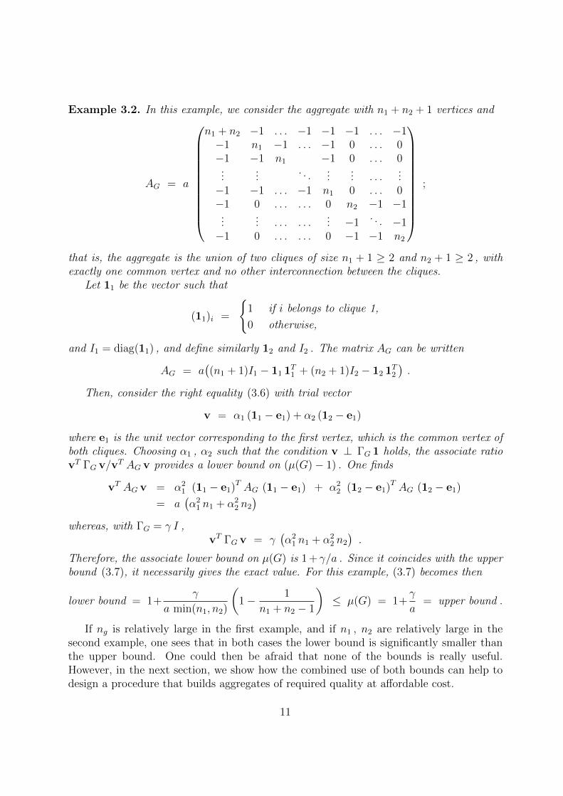
Example 3.2. In this example, we consider the aggregate with n1 + n2 + 1 vertices and

AG = a

n1 + n2 −1 . . . −1 −1 −1 . . . −1−1 n1 −1 . . . −1 0 . . . 0−1 −1 n1 −1 0 . . . 0...

.... . .

...... . . .

...−1 −1 . . . −1 n1 0 . . . 0−1 0 . . . . . . 0 n2 −1 −1...

... . . . . . .... −1

. . . −1−1 0 . . . . . . 0 −1 −1 n2

;

that is, the aggregate is the union of two cliques of size n1 + 1 ≥ 2 and n2 + 1 ≥ 2 , withexactly one common vertex and no other interconnection between the cliques.

Let 11 be the vector such that

(11)i =

{1 if i belongs to clique 1,

0 otherwise,

and I1 = diag(11) , and define similarly 12 and I2 . The matrix AG can be written

AG = a((n1 + 1)I1 − 11 1T

1 + (n2 + 1)I2 − 12 1T2

).

Then, consider the right equality (3.6) with trial vector

v = α1 (11 − e1) + α2 (12 − e1)

where e1 is the unit vector corresponding to the first vertex, which is the common vertex ofboth cliques. Choosing α1 , α2 such that the condition v ⊥ ΓG 1 holds, the associate ratiovT ΓG v/vT AG v provides a lower bound on (µ(G)− 1) . One finds

vT AG v = α21 (11 − e1)T AG (11 − e1) + α2

2 (12 − e1)T AG (12 − e1)

= a(α2

1 n1 + α22 n2

)whereas, with ΓG = γ I ,

vT ΓG v = γ(α2

1 n1 + α22 n2

).

Therefore, the associate lower bound on µ(G) is 1 + γ/a . Since it coincides with the upperbound (3.7), it necessarily gives the exact value. For this example, (3.7) becomes then

lower bound = 1+γ

a min(n1, n2)

(1− 1

n1 + n2 − 1

)≤ µ(G) = 1+

γ

a= upper bound .

If ng is relatively large in the first example, and if n1 , n2 are relatively large in thesecond example, one sees that in both cases the lower bound is significantly smaller thanthe upper bound. One could then be afraid that none of the bounds is really useful.However, in the next section, we show how the combined use of both bounds can help todesign a procedure that builds aggregates of required quality at affordable cost.

11

4 DRA with quality control

In this section, we first recall the DRA algorithm (Section 4.1). Then (Section 4.2), weconsider how to inexpensively check whether the quality measure of a given aggregate isbelow a given threshold. Next (Section 4.3), we explain how, starting from a tentativeaggregate — as, e.g., produced by the DRA algorithm — one can progressively remove“bad” vertices until the quality test is passed. A heuristic strategy to increase meanaggregates size is further discussed (Section 4.4), and the section is concluded with aglobal overview of the proposed approach (Section 4.5).

4.1 DRA algorithm

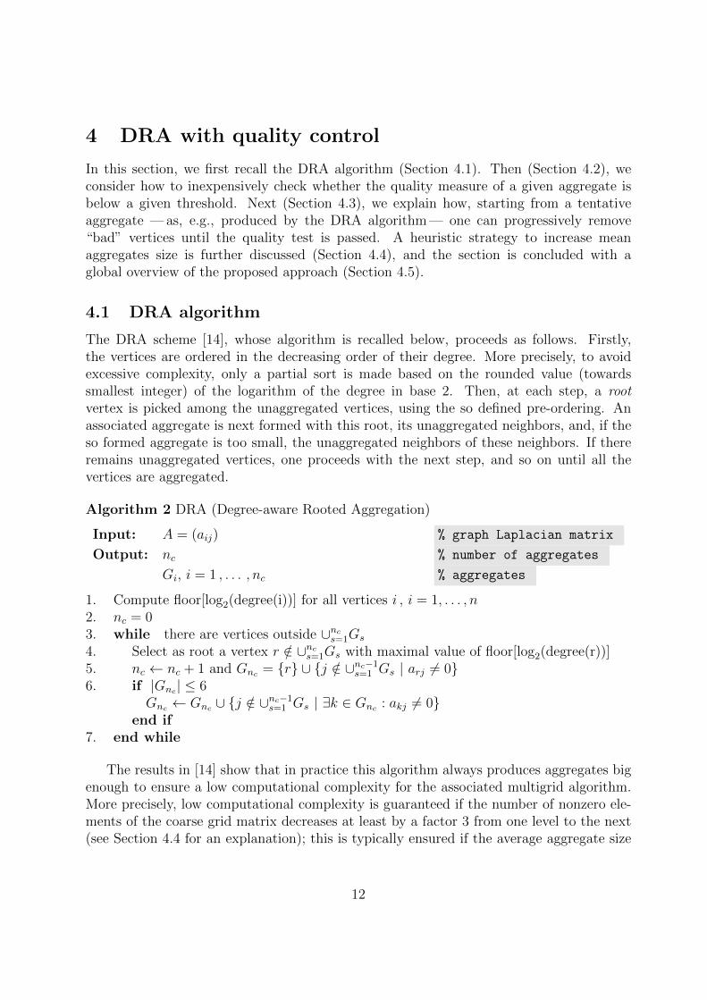
The DRA scheme [14], whose algorithm is recalled below, proceeds as follows. Firstly,the vertices are ordered in the decreasing order of their degree. More precisely, to avoidexcessive complexity, only a partial sort is made based on the rounded value (towardssmallest integer) of the logarithm of the degree in base 2. Then, at each step, a rootvertex is picked among the unaggregated vertices, using the so defined pre-ordering. Anassociated aggregate is next formed with this root, its unaggregated neighbors, and, if theso formed aggregate is too small, the unaggregated neighbors of these neighbors. If thereremains unaggregated vertices, one proceeds with the next step, and so on until all thevertices are aggregated.

Algorithm 2 DRA (Degree-aware Rooted Aggregation)

Input: A = (aij) % graph Laplacian matrix

Output: nc % number of aggregates

Gi, i = 1 , . . . , nc % aggregates

1. Compute floor[log2(degree(i))] for all vertices i , i = 1, . . . , n2. nc = 03. while there are vertices outside ∪nc

s=1Gs

4. Select as root a vertex r /∈ ∪ncs=1Gs with maximal value of floor[log2(degree(r))]

5. nc ← nc + 1 and Gnc = {r} ∪ {j /∈ ∪nc−1s=1 Gs | arj 6= 0}

6. if |Gnc | ≤ 6Gnc ← Gnc ∪ {j /∈ ∪nc−1

s=1 Gs | ∃k ∈ Gnc : akj 6= 0}end if

7. end while

The results in [14] show that in practice this algorithm always produces aggregates bigenough to ensure a low computational complexity for the associated multigrid algorithm.More precisely, low computational complexity is guaranteed if the number of nonzero ele-ments of the coarse grid matrix decreases at least by a factor 3 from one level to the next(see Section 4.4 for an explanation); this is typically ensured if the average aggregate size

12

is at least 4 . The latter requirement motivates the step 6 of the algorithm, which expandssmall root-and-neighbors aggregates. 1

Now, this algorithm does not control the quality of the aggregates, which, as seen in[14], sometimes leads to relatively large two-grid condition numbers.

4.2 Quality tests

Computing µ(G) for a given (tentative) aggregate is too costly to be done repeatedlywithin the setup phase of an AMG method. Fortunately, as observed in [13], an explicitcomputation is not needed to check that µ(G) is below a given threshold κ . It suffices toverify whether the matrix

ZG = κAG −XG(I − 1(1TXG1)−11TXG) (4.1)

is nonnegative definite, which can be done performing a Cholesky factorization. Moreprecisely, if AG has zero row-sum (as always in this work), then ZG has also zero row-sum(and therefore is singular). Then, the last pivot of the Cholesky factorization is alwayszero (in exact arithmetic), and ZG is nonnegative definite if and only if the factorizationof any principal submatrix of size |G| − 1 yields no negative pivot.

We may further use the upper bound in Theorem 3.3 as a sufficient condition. Let rbe the index of the root vertex of G , and let, for all j in G ,

δj =((U −D)D−1(L−D)1

)j, (4.2)

with, as before, U = triu(A) , D = diag(A) and L = tril(A) . From the right inequality(3.7) (considered with i = r) and the definition of ΓG = diag(γj) in Theorem 3.2 one seesthat one will have µ(G) < κ if

2∑

k 6∈G |ajk|+ δj

|ajr|≤ κ− 1 ∀ j ∈ G\{r} . (4.3)

This criterion is useful in two ways. Firstly, when it is met, one may skip the factoriza-tion of the matrix (4.1), and hence save some computing time. Next, and more importantly,in some graphs, there are vertices with thousands of neighbors, for which the DRA algo-rithm will produce huge tentative aggregates (remember that vertices of high degree havepriority for being selected as root vertex). Because the cost of the factorization of thematrix (4.1) is O(|G|3) , we can in fact not afford it when |G| is too large. Then the onlyviable way to guarantee aggregate quality is to use (4.3) as necessary condition, althoughwe know that it is only a sufficient one.

In practice, we observed that the impact of the factorization on the overall computingtime was significant beyond the size of 1024. Hence, when |G| > 1024 , a tentative aggregate

1The expansion size threshold is set to 6 , this value being observed in [14] to deliver on average thebest tradeoff between larger aggregates obtained with larger thresholds, and the better average qualitythat typically results when using smaller thresholds.

13

will be considered passing the quality test only if (4.3) holds (regardless ZG), whereas, if|G| ≤ 1024 , the main criterion is based on the factorization of the matrix ZG in (4.1)(which is skipped only if (4.3) turns out to be satisfied).

Note that (4.3) can be passed only if all vertices are connected to the root vertex(otherwise, some of the |ajr| are zero). This is usually the case for large aggregates producedby the DRA algorithm, since step 6 in Algorithm 2 is skipped when the root vertex has atleast five unaggregated neighbors.

4.3 Aggregate filtering

The probability that an aggregate directly produced by Algorithm 2 passes the quality testis relatively low. However, in most of the cases that we encountered, it turns out possible toextract a reasonably large subset of vertices that form an aggregate of acceptable quality.Here we present the two tools that we use to identify such subset of vertices in a givententative aggregate.

The first tool, presented in Section 4.3.1, detects and removes “bad” vertices; that is,vertices that fail to satisfy given criteria based on the two-sided bound (3.7). This tool issystematically applied to every aggregate produced by the DRA algorithm, before testingexplicitly for quality as explained in the preceding subsection.

The second tool, presented in Section 4.3.2, is applied when the aggregate fails theexplicit quality test based on (4.1). It selects a subgroup of vertices in a way that allowsto properly handle the situations like in Example 3.2.

4.3.1 Bad vertices removal

Our approach is inspired by the two-sided bound (3.7). It is better explained by rewritingthese bounds for the context of Theorem 3.2 (as already done for (4.3) before), with i beingagain set to the root index r of the tentative aggregate G . This gives:

∀j ∈ G\{r} : 1 +2∑

k 6∈G |ajk|+ δj∑k∈Gk 6=j|ajk|

ξj ≤ µ(G) ≤ 1 +2∑

k 6∈G |ajk|+ δj

|ajr|, (4.4)

where

δj =((U −D)D−1(L−D)1

)j

and ξj = 1−2∑

`6∈G |aj`|+ δj∑k∈G

(2∑

` 6∈G |ak`|+ δk

) .

Based on this we decide that a vertex j 6= r should be kept in G if

2∑

k 6∈G |ajk|+ δj

|ajr|≤ κ− 1 (4.5)

or2∑

k 6∈G |ajk|+ δj∑k∈Gk 6=j|ajk|

≤ κ− 1

ηand |G| ≤ 1024 , (4.6)

14

where η > 1 is a security factor (we typically use η = 2). In other words, only thecriterion (4.5) applies for aggregates larger than 1024, while vertices in smaller aggregatesare accepted if they satisfy either (4.5) or (4.6).

The rationale for this is as follows. If all vertices are accepted thanks to the firstcondition (4.5), the inequality (4.3) holds , and hence the aggregate passes the quality test.However, in view of Example 3.1, it would be too restrictive to use this sole condition, atleast when |G| ≤ 1024 , so that the aggregate has a chance to pass the quality test when(4.3) does not hold. This motivates the second criterion (4.6), which disregards the upperbound, but tends to ensure that the lower bound on µ(G) is significantly below the largestadmissible value (we neglect the factor ξj , the approach being heuristic, anyway). Observealso that, apart from the term δj , this criterion is essentially a constraint on the ratio∑

k 6∈G |ajk|∑k∈Gk 6=j|ajk|

; (4.7)

that is, on the sum of the weights of external connections divided by the sum of the weightsof internal connections. Intuitively, the smaller this ratio, the larger is the probability thatthe vertex is a “good” aggregate member.

From a practical viewpoint, it is worth noting that the removal of a vertex from Gpossibly implies, for the vertices j still in G , an increase of

∑k 6∈G |ajk| and decrease of∑

k∈G,k 6=j |ajk| . This negatively affects the satisfaction of the criteria (4.5) and (4.6). Totake this into account, we continuously sweep through the vertices of an aggregate, assessing(4.5) and (4.6) based on the most recent tentative aggregate G , and stopping only oncea complete sweep has been achieved without any removal. In practice, we observed thatthe number of times each vertex is visited during this procedure is most often between 2and 4.

4.3.2 Subgroup extraction

Here we consider the treatment of tentative aggregates issued from the just exposed removalprocedure, but that nevertheless fail the quality test based on the factorization of (4.1).Such aggregates necessarily contain vertices accepted thanks to (4.6). Hence a furtherfiltering is possible by increasing the security factor η to make this criterion more stringent.However, in view of situations like that of Example 3.2, this is not always sufficient.

This motivates the subgroup extraction technique presented here, which exploits thefact that the cases we are interested in are those where the Cholesky factorization of ZG in(4.1) has broken down. As a by-product of the factorization, one can inexpensively retrievea vector w such that

wT ZG w = p < 0 ,

where p is the encountered negative pivot. Because ZG is symmetric and ZG 1 = 0 , wehave as well

(w + α 1)T ZG (w + α 1) = p

15

for any α , thus also for v = w + α 1 satisfying 1T XG v = 0 . For this specific vector wehave (see (4.1))

p = vT ZG v = κ vT AG v − vT XG v = (κ− 1) vT AG v − vT ΓG v,

where ΓG = XG − AG . Hence:

1 +vT ΓG v

vT AG v= κ− p

vT AG v> κ .

Remembering that 1T XG v = 0 and, therefore, 1T ΓG v = 0 (here 1TΓG is always nonzero ifµ(G) > 1) , the vector v may be seen as an approximation of arg maxv⊥ΓG 1(vT ΓG v/vT AG v)which provides the exact value of µ(G) ; see (3.6). On the other hand, as noted in the proofof Theorem 3.3, this latter is the eigenvector associated with the second smallest eigenvalueof the generalized eigenvalue problem

AG z = λ XG z . (4.8)

This eigenvector may be seen as a generalized Fielder vector. Since the sign of the entriesin the Fiedler vector is often used for graph partitioning, this motivates us in discriminatingaggregate members based on the sign of the corresponding entry in v . More precisely, weproceed as follows. We pre-select as remaining aggregate members all vertices for whichthe component in v has the same sign as that of the root vertex. Letting Gp be the setof pre-selected vertices, we then effectively keep in the tentative aggregate G the verticesother than root such that

2∑

k 6∈Gp

k 6=j

|ajk|+ δj

|ajr|≤ κ− 1 or

2∑

k 6∈Gp

k 6=j

|ajk|+ δj∑k∈Gp

k 6=j

|ajk|≤ κ− 1

η. (4.9)

Note that, in this way, the vertices not initially pre-selected (i.e., those in G\Gp) can finallystay in the tentative aggregate; i.e., we avoid a too crude decision based on the sole signsin v .

Once this new tentative aggregate has been obtained, it will undergo the bad ver-tices removal procedure described in the preceding subsection, before a new quality testis performed. It may then re-enter the procedure described here only in case of a newfactorization failure, which turns out to be extremely rare.

The following example illustrates how the subgroup extraction works and can success-fully face situations like that of Example 3.2.

Example 4.1. We consider a particular instance of Example 3.2, with n1 = 10 andn2 = 12 , except that some randomly chosen edges have been removed; see Figure 1 (left).To make the case more realistic, a random reordering of the vertices is applied, and theconnectivity pattern of the tentative aggregate is as illustrated on Figure 1 (right). All

16

weights are equal to one, and the diagonal of ΓG is filled with random numbers uniformlydistributed in (0, 25) :(

2∑k 6∈G

|ajk|+δj

)j=1,...,21

=(

7.4 13.3 4.8 1.7 19.7 16.4 15.9 14.4 1.0 8.9 23.6

1.5 21.6 21.9 1.3 16.3 13.8 14.9 12.1 7.1 7.4)

It turns out that the largest value for the ratio in the left hand side of (4.6) is 3.7 , whichis below (κ− 1)/η for the standard values κ = 10 and η = 2 .

Hence, the aggregate passes the “bad vertices removal” procedure described in Sec-tion 4.3.1 without any vertex removed. However, the factorization of the matrix (4.1)yields a negative pivot. The corresponding vector v is

v =(

- 0.24 0.88 - 1.16 - 1.09 1.09 1.29 - 1.32 - 1.24 0.60 0.99 1.04

- 1.12 - 1.44 1.42 - 1.13 - 1.36 0.85 0.01 - 1.00 - 1.00 - 1.00).

One may check that it satisfies the proper orthogonality condition. On the other hand,

1 +vT ΓG v

vT AG v= 11.2 ,

whereas a numerical computation reveals that µ(G) = 14.4 . Moreover, v is relatively closeto the eigenvector z2 associated with the second smallest eigenvalue of (4.8), since we obtain

cos(v , z2) = 0.97 .

Further, the pre-selection based on the sign of the entries in v yields the result illustratedin Figure 2 (left). In fact, Gp is precisely the set of vertices belonging to the second groupof vertices, as is better seen looking at Figure 2 (right).

It follows that the test (4.9) yields the same discrimination as the test based on thesigns in v , hence Gp is also the new tentative aggregate we restart the bad vertices re-moval procedure with. Moreover, all vertices satisfy (4.6) (the values of the ratio (4.7)are unchanged from the previous step), whereas the factorization test is here successful.Hence, Gp is the finally accepted aggregate. A further numerical computation reveals thatµ(Gp) = 4.2 , which is indeed below κ = 10 and about 3.5 times smaller than the initialvalue µ(G) = 14.4 .

4.4 Enhancing complexity

As stated in the Introduction (see also Section 4.1), one of the attractive features of theDRA algorithm lies in its ability to produce “large enough” aggregates independently ofthe connectivity pattern of the graph. Clearly, the quality control may have a negativeimpact on aggregates size, which needs to be investigated before going further.

17

Figure 1: Sparsity pattern of the Laplacian matrix AG associated to the aggregate Gfrom Example 4.1; left and right figures represent the pattern before and after a randomreordering of the vertices, respectively.

Figure 2: Same as Figures 1 (in reversed order), but with entries corresponding to Gp beingmarked with red circles.

To develop the discussion, it is useful to recall how aggregates size is related withthe complexity of the multigrid algorithm. Because we use the K-cycle, the work periteration and the memory requirements are controlled, respectively, through the weightedand operator complexities [13, 14], defined by

CW = 1 +L∑

`=2

2`−1 nnz(A`)

nnz(A)and CA = 1 +

L∑`=2

nnz(A`)

nnz(A), (4.10)

18

where A1 = A and where A2 , . . . , AL are the successive coarse grid matrices, L being thenumber of levels. More precisely, CW indicates the cost of the preconditioner applicationrelative to the cost of smoothing iterations at fine grid level, whereas CA provides thememory needed to store the preconditioner relative to that needed for the system matrixA . Note that in our case the cost of smoothing iterations at fine grid level, including theresidual updates at step 2 and 6 of Algorithm 1, is equal to2 the cost of 2.5 matrix-vectorproducts by the matrix A . Both parameters are kept under control by ensuring that

nnz(A`−1)/nnz(A`) ≥ τ, ` = 2 , . . . , L ,

with τ well beyond 2; for instance, if τ = 3, then CW ≤ 3 and CA ≤ 3/2 .Clearly, larger aggregates imply smaller coarse grid matrices with, on average, less

nonzero entries; i.e., larger coarsening ratios nnz(A`−1)/nnz(A`) . When we state thatthe DRA algorithm produces “large enough” aggregates, we mean that it consistentlysucceeds to achieve low weighted and operator complexities, the coarsening ratios beingnever significantly below 3 [14]. Regarding the quality control, we therefore need to checkwhether or not it has a significant impact on these ratios.

In this regard, one may consider the first two groups of columns in Table 1 (the thirdgroup is commented later on), where relevant quantities are shown for a sample of sixtest problems that are representative of the different situations met in practice. With nosurprise, when using the DRA algorithm alone, the coarsening ratios are always above 3but the condition number is sometimes large, whereas, adding the quality control, somecoarsening ratios become small, while, in agreement with the theory, the condition numberis always below the prescribed limit κ = 10 .

Going to the details, the first two problems are representative of situations where thequality control has little impact: the condition number is already nice without it, and,despite the coarsening ratio is significantly reduced, it is still far above the limit thatguarantees low complexities. The third and fourth problems show cases where the conditionnumber is significantly improved thanks to the quality control, while the impact on thecoarsening speed is again marginal. The difficult cases are represented by the fifth andsixth problems. In the fifth one, one would better skip the quality control, since it hasonly a marginal effect on the already nice condition number, but has a dramatic impacton the coarsening ratio. The situation is more mixed in the sixth case, where the qualitycontrol brings the needed improvement of the condition number, whereas the coarseningratio, although small, is not that small.

To improve the situation when the coarsening ratio becomes small while keeping (hope-fully) most of the benefit of the quality control, we then propose the following strategy.If, after the DRA algorithm with control has completed, it turns out that the ratio n/nc

between the number of variables and the number of aggregates is below 4, 3 then the ver-tices of aggregates of size 3 or less are marked as unaggregated, and the DRA aggregation

2The value 2.5 takes into account the solution steps 1 and 7 of Algorithm 1 as well as the residualevaluation at steps 2 and 6, the former evaluation being performed via r = (D − U)v1 with U = triu(A)and D = diag(A).

3this ratio is also the mean aggregate size

19

DRA DRA-QC DRA-QC-CE

Graph κeffnnc

nnz(A)nnz(A2)

κeffnnc

nnz(A)nnz(A2)

κeffnnc

nnz(A)nnz(A2)

bcsstk29‡ 2.8 19.8 121.6 2.3 5.7 14.1 (2.3) (5.7) (14.1)nopoly† 6.7 7.1 8.0 6.0 4.8 5.0 (6.0) (4.8) (5.0)

Oregon-2†lcc 4.7 3.6 6.1 2.1 10.0 5.8 (2.1) (10.0) (5.8)

web-NotreDame‡lcc 58.2 13.4 12.3 7.2 13.1 8.5 (7.2) (13.1) (8.5)

t60k† ‡ 4.0 4.1 3.0 3.5 2.2 1.7 3.8 4.9 2.9

web-BerkStan‡lcc 85.5 15.8 52.3 8.8 3.2 2.9 18.2 13.7 27.8

Table 1: Condition number and coarsening ratios for a two-grid method when using theDRA algorithm alone (DRA), the DRA algorithm with quality control (DRA-QC), andthe DRA algorithm with both quality control and complexity enhancement (DRA-QC-CE);dagger symbol † informs that the Laplacian matrix of the graph comes from the Universityof Florida Sparse Matrix Collection [7]; double dagger ‡ is for matrices from the LAMGtest set suite [10]; the subscript lcc means that the experiment was performed with thelargest connected component of the matrix; nc represents the number of rows and columnsof A2 ; that is, the number of aggregates.

procedure is applied to them without any quality control — the aggregates of size 4 ormore obtained during the first pass being kept unchanged. Note that the decision is basedon the ratio n/nc because the coarsening ratio (based on the number of nonzero entries)is known only when the coarse grid matrix is formed, which is usually done only afterthe aggregation has been finalized. On the other hand, satisfactory complexity values aretypically obtained if the ratio n/nc is above 4 (see Table 1 for illustration); this in turnexplains the threshold value.

This strategy, referred to as DRA with quality control and complexity enhancement(DRA-QC-CE), is illustrated with the last group of columns in Table 1. In the first fourproblems, the ratio n/nc is above the target, hence no extra step is performed, and theresults are the same as for DRA with quality control. The extra step is performed inthe remaining two cases, and one may observe that the coarsening ratios become indeedacceptable. More precisely, in the fifth problem, one actually recovers almost the situationone had without quality control, and which is optimal in this case. In the last problem,one gets in some sense the best of two worlds: the coarsening ratio is pretty large as itwas without quality control, but the condition number, although above the limit κ = 10 ,remains far below the one obtained without quality control.

4.5 Summary

We summarize the resulting aggregation scheme with the Algorithm 3 below. The aggre-gates are initially formed as in Algorithm 2 above (steps 4–6): first a root vertex is chosenamong those with the highest value of floor[log2(degree)] ; then the neighboring vertices

20

are added and, if the aggregate size is at most 6 , neighbors of neighbors are appended.However, unlike in Algorithm 2, the resulting aggregates are only tentative. They

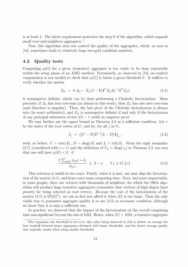
further undergo the bad vertices removal described in Section 4.3.1 (step 10). Next, theaggregates are tested for quality, firstly via the criterion (4.3) (step 11), and, if needed,via the factorization of the matrix ZG in (4.1) (step 12) — as written above, this is in factnever done when the size of the tentative aggregate is above 1024 , since then the removalprocedure only keeps vertices satisfying (4.5). If the factorization of ZG yields a negativepivot, the subgraph extraction tool described in Section 4.3.2 is further applied (steps 13–16). The resulting new tentative aggregate then reenters the procedure at step 9; i.e., badvertices removal is again applied (with a slightly larger value of η) before a new explicitquality test based on (4.1). And so on, until the tentative aggregate G satisfies either theupper bound (4.3) (step 11) or the explicit quality criterion based on (4.1) (step 12); ineither case it satisfies µ(G) < κ when it is accepted (step 19).

Eventually, after all vertices have been assigned to an aggregate with verified quality,we check if the number of coarse variables (i.e., the number of aggregates) is at least 4times smaller than the number of vertices (step 21). If not, the complexity enhancementprocedure described in Section 4.4 is applied (steps 22–24); that is, small aggregates aredeleted, and the DRA algorithm without control is executed to group the so releasedvertices into additional aggregates.

Algorithm 3 DRA-QC-CE (DRA with quality control and complexity enhancement)

Input: A = (aij) % a graph Laplacian matrix

κ % quality threshold (here set to 10)

Output: nc % number of aggregates

Gi, i = 1 , . . . , nc % aggregates

1. Compute floor[log2(degree(i))] for all vertices i , i = 1, . . . , n2. nc = 03. while there are vertices outside ∪nc

s=1Gs

% compute next tentative aggregates using DRA (steps 4-6)

4. Select as root a vertex r /∈ ∪ncs=1Gs with maximal value of floor[log2(degree(r))]

5. G = {r} ∪ {j /∈ ∪ncs=1Gs | arj 6= 0}

6. if |G| ≤ 6G← G ∪ {j /∈ ∪nc

s=1Gs | ∃k ∈ G : akj 6= 0}end if

% extract a good-quality aggregate (steps 7-18)

7. η ← 28. accept ← false9. while not accept

cleaned ← false

% filter bad vertices (step 10)

21

10. while not cleanedcleaned ← truefor j ∈ G , j 6= r

if criteria (4.5) and (4.6) not satisfied for jG← G\{j}cleaned ← false

end ifend for

end while

% test quality (steps 11, 12)

11. if criterion (4.3) is satisfiedaccept ← true

else12. if Cholesky factorization of ZG defined by (4.1) fails

% subgraph extraction (steps 13-16)

13. η ← η + 0.514. Gp ← {j ∈ G |v(j) v(r) ≥ 0} with v as defined in Section 4.3.215. if v(r) = 0 : Gp ← {j ∈ G |v(j) ≥ 0} end if16. G← {j ∈ G |j = r or criterion (4.9) satisfied with respect to Gp}17. else

accept ← trueend if

end if18. end while

% form aggregate (step 19)

19. nc ← nc + 1 and Gnc ← G20. end while

% if needed, reform small aggregates (steps 21-25)

21. if nc > n/422. delete all Gj such that |Gj| ≤ 3 ;23. reset nc equal to the number of non deleted aggregates;24. add aggregates obtained by running Algorithm 2 from step 3 with

Gj , j = 1, . . . , nc being the non deleted aggregates25. end if

5 Numerical experiments

We begin by describing in Section 5.1 the extensive test set used for the experiments,providing details of the experimental setting, and commenting on the representation ofthe reported results. We then assess the new method in Section 5.2, comparing with the

22

former variant without quality control. Eventually, we provide in Section 5.3 a comparisonwith the LAMG solver from [11].

5.1 General setting

The experiments have been performed on all the graph Laplacian matrices of undirectedgraphs that come from either The University of Florida Sparse Matrix Collection [7] orthe LAMG test set suite [10]. In both cases, only the graphs with more than 104 verticesand with limited variation of edge weights have been considered. This gave a total of 142graphs. For graphs with several connected components, the tests were run on the largestcomponent.

The elapsed time is reported only for the 113 graphs that have more than 2·105 nonzeroentries in their Laplacian matrix. (The elapsed times for the remaining 29 graphs are toosmall, and hence subject to large relative variations from run to run.) Time experimentswere performed by running a Fortran 90 implementation of the method on a single coreof a computing node with two Intel XEON L5420 processors at 2.50 GHz and 16 Gb RAMmemory. When considering the absolute value of the reported times, it is good to rememberthat this machine dates back to 2009.

In all cases, we used the flexible conjugate gradient method (FCG(1)) with the zerovector as initial approximation, the stopping criterion being 10−6 reduction in the resid-ual norm. Right hand sides were generated randomly, the compatibility condition beingenforced by an explicit projection onto R(A) = 1⊥ .

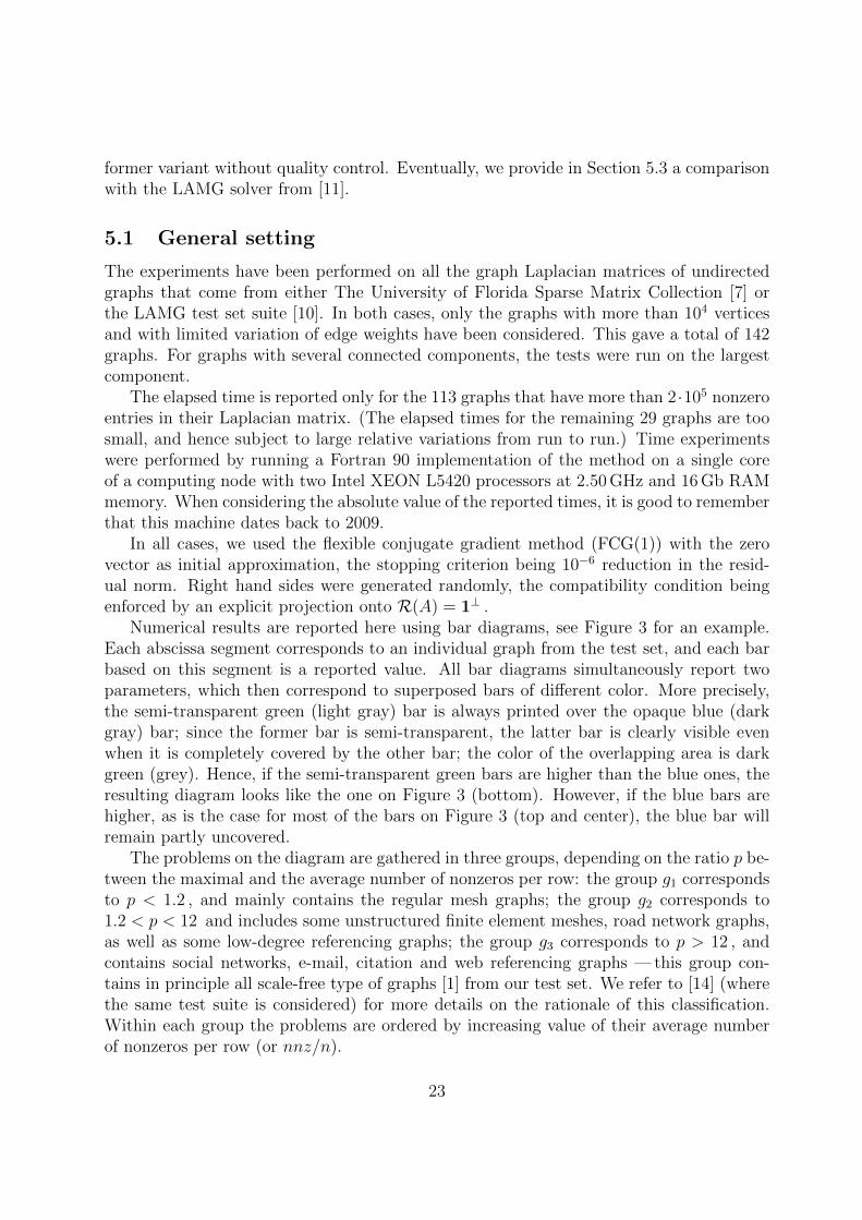
Numerical results are reported here using bar diagrams, see Figure 3 for an example.Each abscissa segment corresponds to an individual graph from the test set, and each barbased on this segment is a reported value. All bar diagrams simultaneously report twoparameters, which then correspond to superposed bars of different color. More precisely,the semi-transparent green (light gray) bar is always printed over the opaque blue (darkgray) bar; since the former bar is semi-transparent, the latter bar is clearly visible evenwhen it is completely covered by the other bar; the color of the overlapping area is darkgreen (grey). Hence, if the semi-transparent green bars are higher than the blue ones, theresulting diagram looks like the one on Figure 3 (bottom). However, if the blue bars arehigher, as is the case for most of the bars on Figure 3 (top and center), the blue bar willremain partly uncovered.

The problems on the diagram are gathered in three groups, depending on the ratio p be-tween the maximal and the average number of nonzeros per row: the group g1 correspondsto p < 1.2 , and mainly contains the regular mesh graphs; the group g2 corresponds to1.2 < p < 12 and includes some unstructured finite element meshes, road network graphs,as well as some low-degree referencing graphs; the group g3 corresponds to p > 12 , andcontains social networks, e-mail, citation and web referencing graphs — this group con-tains in principle all scale-free type of graphs [1] from our test set. We refer to [14] (wherethe same test suite is considered) for more details on the rationale of this classification.Within each group the problems are ordered by increasing value of their average numberof nonzeros per row (or nnz/n).

23

5.2 Assessment of the new method

Let us first summarize how the ingredients of the new method are combined. It first recur-sively eliminates all the vertices of degree 1 in the system matrix, yielding a reduced Schurcomplement system (this applies only to graphs having such vertices, and the importanceof this preprocessing step is discussed in [14]). This system is solved with FCG(1), using

the preconditioner defined by Algorithm 1, in which step 4 is modified when n`+1 > n1/31 ,

the vertices of degree 1 being first eliminated, and the reduced Schur complement sys-tem being approximately solved with 2 FCG(1) using the same two-grid preconditionerat this coarse level. The aggregates Gi , i = 1, . . . , nc used at each level are obtainedwith the DRA-QC-EC algorithm (Algorithm 3) applied to the Schur complement matrixresulting from the elimination of degree 1 vertices. The only difference with the method in[14] lies in this use of the DRA-QC-EC algorithm instead of the original DRA algorithm(Algorithm 2).

The difference between both methods is illustrated in Figure 3, where we display theweighted and operator complexities as defined by (4.10), as well as the number of iter-ations needed to solve the test problems. The results are along the lines expected fromthe discussion in the preceding section. On the one hand, thanks, in some cases, to thecomplexity enhancement, the impact of the quality control on the complexities is fairlymoderate, and, in particular, the weighted complexity remains below 3 as desired. On theother hand, the quality control clearly brings the robustness it has been designed for, thenumber of iterations being stabilized in the interval 15− 30 independently of the problem.

The timing results are displayed in Figure 4 in seconds per million of nonzeros. Thenew aggregation algorithm is significantly more costly during the setup phase, but thesetup time remains fairly low in absolute value, exceeding rarely and never dramaticallyhalf of a second per million of nonzero. Regarding the solve times, they are very closeto each other in roughly two thirds of the problems, whereas the new method brings asignificant improvement in the remaining third. Hence it is always a good idea to usethe new DRA-QC-CE algorithm when emphasis is on the solve time, for instance becauseseveral systems have to be solved with the same matrix. For one shot applications, theresults are more mixed, as illustrated with the reported total times.

5.3 Comparison with LAMG

We now report on the comparison between the solver based on the new aggregation schemeand the LAMG solver [10] implementing the method by Livne and Brandt [11]. The mainLAMG driver is a Matlab function, but computationally intensive routines are written inC. The code was run on a single computing node, using the standard Matlab environment.Note that [11], regarding numerical experiments, mainly reports timing results, leading tothink that the LAMG code has been enough optimized with respect to speed, and hencethat a comparison with our code based on time measurements is reasonably fair althoughprogramming languages are different.

Timing results are displayed in Figure 5. Up to a few exceptions, both the setup and

24

0

1

2

3

g1 g2 g3

com

ple

xit

y

DRA (CW )new (CW )(bars overlap)

0

1

2

g1 g2 g3

com

ple

xit

iy

DRA (CA)new (CA)(bars overlap)

0

25

50

75

g1 g2 g3

#it

DRA (#it)new (#it)(bars overlap)

Figure 3: Weighted (top) and operator (center) complexities, as well as iteration counts(bottom) for the solver [14] based on DRA and on the new DRA-QC-EC aggregationscheme. The test problems are gathered in three groups – g1 , g2 and g3 – as described inthe end of Section 5.1; consecutive groups are separated with a dashed line.

25

0

0.4

0.8

1.2

g1 g2 g3

tim

e/n

nz

(sec

ond

sp

erm

illi

onof

non

zero

s)

DRA (setup)new (setup)(bars overlap)

0

1

2

g1 g2 g3

tim

e/n

nz

(sec

ond

sp

erm

illion

ofn

on

zero

s)

DRA (solve)new (solve)(bars overlap)

0

1

2

3

g1 g2 g3

tim

e/n

nz

(sec

ond

sp

erm

illion

ofn

onze

ros)

DRA (total)new (total)(bars overlap)

Figure 4: Setup (top), solution (center) and total time (bottom) for the solvers based onDRA and on the new DRA-QC-EC aggregation scheme; only graph Laplacians with morethan 2 · 105 nonzero entries are considered. 26

solution times are lower for the new solver and, as a result, the total times are also typically2 to 3 times lower. In fact, LAMG is mainly better for graphs with few nonzero entriesper row. Most of these graphs correspond to road networks with the number of nonzeroentries per row below 4, meaning that the average degree of the vertices is below 3. Inthese cases, LAMG benefits from an extended preprocessing step, that eliminates verticeswith degree up to 4, whereas our methods only eliminates vertices of degree 1. Such anextended elimination is thus worth considering if the focus is on graphs with very smallaverage degree.

6 Conclusions

We considered the solution of graph Laplacian systems with aggregation-based multigrid.We incorporated quality control in the DRA algorithm proposed in [14] in order to improveits robustness. Moreover, we successfully faced the two inherent obstacles. Firstly, weavoided an excessive increase of the setup time thanks to a clever filtering procedure thatextracts an aggregate of verified quality from a given tentative aggregate without usingany time consuming step. Secondly, we avoided a dramatic impact on the complexity byrunning, in case of need, a second pass where vertices in too small aggregates (of size 1, 2or 3) are regrouped in bigger ones. This results in a new aggregation scheme, referred toas DRA-QC-CE (Degree-aware Rooted Aggregation with quality control and complexityenhancement).

The numerical results demonstrate the robustness and effectiveness of the solver basedon this new aggregation scheme: the number of iterations needed for a six orders of mag-nitude reduction in the residual norm remains below 33 for all the 142 graphs in theconsidered test set. The new solver also compares favorably to the LAMG solver [10],being significantly faster in most cases, whereas, in the few cases where LAMG is better,it only brings a relatively marginal improvement.

References

[1] A.-L. Barabasi and R. Albert, Emergence of scaling in random networks, Science,286 (1999), pp. 509–512.

[2] A. Ben Israel and T. N. E. Greville, Generalized Inverses: Theory and Appli-cations, John Wiley and Sons, New York, 1974.

[3] A. Berman and R. J. Plemmons, Nonnegative Matrices in the Mathematical Sci-ences, Academic Press, New York, 1979.

[4] M. Bolten, S. Friedhoff, A. Frommer, M. Heming, and K. Kahl, Alge-braic multigrid methods for Laplacians of graphs, Linear Algegra Appl., 434 (2011),pp. 2225–2243.

27

0

1

2

3

g1 g2 g3

tim

e/n

nz

(sec

ond

sp

erm

illi

on

ofn

on

zero

s)

LAMG (setup)new (setup)(bars overlap)

0

2

4

6

g1 g2 g3

tim

e/n

nz

(sec

ond

sp

erm

illi

onof

non

zero

s)

LAMG (solve)new (solve)(bars overlap)

0

3

6

9

g1 g2 g3

tim

e/n

nz

(sec

ond

sp

erm

illi

onof

non

zero

s)

LAMG (total)new (total)(bars overlap)

Figure 5: Setup (top), solution (center) and total time (bottom) for the solvers based onthe new DRA-QC-EC aggregation scheme and for the LAMG code; only graph Laplacianswith more than 2 · 105 nonzero entries are considered.28

[5] E. G. Boman and B. Hendrickson, Support theory for preconditioning, SIAM J.Matrix Anal. Appl., 25 (2003), pp. 694–717.

[6] A. Brandt, S. F. McCormick, and J. W. Ruge, Algebraic multigrid (amg) forsparse matrix equations, in Sparsity and its Application, D. J. Evans, ed., CambridgeUniversity Press, Cambridge, 1984, pp. 257–284.

[7] T. A. Davis and Y. Hu, The University of Florida Sparse Matrix Collection, ACMTrans. Math. Software, 38 (2011), pp. 87–94.Available via http://www.cise.ufl.edu/research/sparse/matrices/.

[8] R. D. Falgout and P. S. Vassilevski, On generalizing the algebraic multigridframework, SIAM J. Numer. Anal., 42 (2005), pp. 1669–1693.

[9] I. Koutis, G. L. Miller, and D. Tolliver, Combinatorial preconditioners andmultilevel solvers for problems in computer vision and image processing, ComputerVision and Image Understanding, 115 (2011), pp. 1638–1646.

[10] O. E. Livne, Lean Algebraic Multigrid (LAMG) matlab software, 2012. Release 2.1.1.Freely available at http://lamg.googlecode.com.

[11] O. E. Livne and A. Brandt, Lean Algebraic Multigrid (LAMG): Fast graph Lapla-cian linear solver, SIAM J. Sci. Comput., 34 (2012), pp. B449–B522.

[12] A. Napov and Y. Notay, Algebraic analysis of aggregation-based multigrid, Numer.Lin. Alg. Appl., 18 (2011), pp. 539–564.

[13] , An algebraic multigrid method with guaranteed convergence rate, SIAM J. Sci.Comput., 43 (2012), pp. A1079–A1109.

[14] , An efficient multigrid method for graph Laplacian systems, Electronic Transac-tions on Numerical Analysis, 45 (2016), pp. 201–218.

[15] Y. Notay, Flexible conjugate gradients, SIAM J. Sci. Comput., 22 (2000), pp. 1444–1460.

[16] , An aggregation-based algebraic multigrid method, Electronic Transactions onNumerical Analysis, 37 (2010), pp. 123–146.

[17] , Algebraic two-level convergence theory for singular systems, SIAM J. MatrixAnal. Appl., 37 (2016), pp. 1419–1439.

[18] Y. Notay and P. S. Vassilevski, Recursive Krylov-based multigrid cycles, Numer.Lin. Alg. Appl., 15 (2008), pp. 473–487.

[19] J. W. Ruge and K. Stuben, Algebraic multigrid (AMG), in Multigrid Methods,S. F. McCormick, ed., vol. 3 of Frontiers in Applied Mathematics, SIAM, Philadelphia,PA, 1987, pp. 73–130.

29

[20] D. A. Spielman, Algorithms, graph theory, and linear equations in Laplacian matri-ces, in Proceedings of the International Congress of Mathematicians, vol. IV, WorldScientific, 2010, pp. 2698–2722.

[21] P. M. Vaidya, Solving linear equations with symmetric diagonally dominant matricesby constructing good preconditioners. Unpublished manuscript.

[22] P. Vanek, J. Mandel, and M. Brezina, Algebraic multigrid based on smoothedaggregation for second and fourth order problems, Computing, 56 (1996), pp. 179–196.

[23] P. S. Vassilevski, Multilevel Block Factorization Preconditioners, Springer, NewYork, 2008.

30