Embed Size (px)
Citation preview

Dynamics of Electrodynamic
Tether Systems
Matthew S. Bitzer, Joshua R. Ellis and
Christopher D. Hall
Aerospace and Ocean Engineering
Virginia Tech
Matthew S. Bitzer, Joshua R. Ellis and
Christopher D. Hall
Aerospace and Ocean Engineering
Virginia Tech
Presentation at Presentation at

Where We Are
27,000 students27,000 students27,000 students27,000 students
2600260026002600----acre main campusacre main campusacre main campusacre main campus
>100 buildings>100 buildings>100 buildings>100 buildings

Space-Related Research @

Space-Related Research @

On Research Project Selection
He had been Eight Years upon a Project for extracting Sun-Beams out of Cucumbers, which were to be put into Vials hermetically sealed, and let out to warm the Air in raw inclement Summers. He told me he did not doubt in Eight Years more he should be able to supply the Governors Gardens with Sun-shine at a reasonable Rate.
-- Gulliver, Gulliver’s Travels
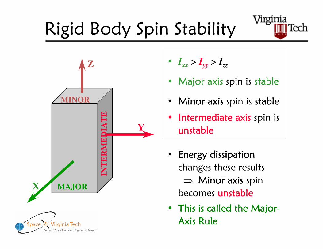
Rigid Body Spin Stability
X
Y
Z • Ixx > Iyy > Izz
• Major axisMajor axisMajor axisMajor axis spin is stablestablestablestable
• Minor axisMinor axisMinor axisMinor axis spin is stablestablestablestable
• Intermediate axisIntermediate axisIntermediate axisIntermediate axis spin is
unstableunstableunstableunstable
• Energy dissipationEnergy dissipationEnergy dissipationEnergy dissipation
changes these results
⇒ Minor axisMinor axisMinor axisMinor axis spin
becomes unstableunstableunstableunstable
• This is called the MajorThis is called the MajorThis is called the MajorThis is called the Major----
Axis RuleAxis RuleAxis RuleAxis Rule
MAJOR
INT
ER
ME
DIA
TE
MINOR

Sputnik & Explorer I
• Sputnik was launched 50 years ago!
• Professor Ronald Bracewell, a radio
astronomer at Stanford, deduced that
Sputnik was spinning about a symmetry axis,
and that it must be the major axis
• He called JPL to make sure that the Explorer I design was taking this into
account, but security prevented him from getting through
• Explorer I was designed as a minor axis spinner, launched in 1958

Spin-Stabilized Satellites
Explorer I (1958) was supposed
to be spin-stabilized about its
minor axis. It went into a flat
spin due to energy dissipation.Telstar I (1962) was spin-
stabilized about its major axis,
spinning at about 200 RPM.

Electrodynamic Tethers
Current inCurrent inCurrent inCurrent in tether tether tether tether
interacts with interacts with interacts with interacts with
earthearthearthearth’’’’s magnetic s magnetic s magnetic s magnetic
field to create a field to create a field to create a field to create a
Lorentz ForceLorentz ForceLorentz ForceLorentz Force Electron collectors Electron collectors Electron collectors Electron collectors
and emitters at and emitters at and emitters at and emitters at
each end of the each end of the each end of the each end of the
tether exchange tether exchange tether exchange tether exchange
free electrons in free electrons in free electrons in free electrons in
the ambient the ambient the ambient the ambient
plasma complete plasma complete plasma complete plasma complete
the tether circuit.the tether circuit.the tether circuit.the tether circuit.

Velocity
Curr
ent
Force
B
Force
BLiF
×=
[1]
Electrodynamic Tethers

Electrodynamic Tethers
F l Bid= ×∫
B
i

EDT System Model
• Two gyrostat end bodies with arbitrary number of momentum wheels and thrusters
• Flexible tether modeled as elastic string, Linear Kelvin-Voigt Law of Viscoelasticity
• Earth-centered, Earth-fixed, tilted dipole model for magnetic field
• Two gyrostat end bodies with arbitrary number of momentum wheels and thrusters
• Flexible tether modeled as elastic string, Linear Kelvin-Voigt Law of Viscoelasticity
• Earth-centered, Earth-fixed, tilted dipole model for magnetic field
n1
n2
n3
o3
o1o
2
a3
a1 a2
e3
b3
b1
b2
Body A
Body B
Ω
ω ν+I
Ar
u
r

Coordinate Frames
FN: inertial frame (similar to perifocal frame)
FO: orbital frame
FA: Body A body frame
FB: Body B body frame
FE: tether-fixed frame
FN: inertial frame (similar to perifocal frame)
FO: orbital frame
FA: Body A body frame
FB: Body B body frame
FE: tether-fixed frame
3e
1e
2e
GA
GB
ˆ1a
ˆ2a
ˆ3a
ˆ1
bˆ2b
ˆ3
b
( )s,tr
Ap
Bp
3e
ds
θ
φ
rABody A
Body B
GA
PA
GB
PB
O
ˆ1
n
ˆ2
n
ˆ3
n
ˆ1o
ˆ2
o
ˆ3o
2-1 rotation sequence through α,β from FO to FE
2-1 rotation sequence through α,β from FO to FE

Solution Methods
• Two different solution methods used for
the tether partial differential equations
– Assumed Modes Assumed Modes Assumed Modes Assumed Modes – tether displacments are
expanded using assumed mode functions
– Finite Element Method Finite Element Method Finite Element Method Finite Element Method – nodal displacements
and slopes interpolated using cubic Hermite
polynomials

Assumed Modes
Expand tether displacements using assumed mode
functions
Expand tether displacements using assumed mode
functions
Express tether position vector relative to E frameExpress tether position vector relative to E frame
Use Galerkin Method to obtain set of 2NT+NLODEs for generalized coordinates
Use Galerkin Method to obtain set of 2NT+NLODEs for generalized coordinates

Finite Elements
Express tether position vector relative to E frameExpress tether position vector relative to E frame
Use interpolation functions to express tether
displacements
Use interpolation functions to express tether
displacements
Shape functions are cubic Hermite polynomials –
ensures continuity of displacement and slope
Shape functions are cubic Hermite polynomials –
ensures continuity of displacement and slope

• Borrowing a technique from
Computational Fluid Dynamics (CFD)…
• Introduce additional terms into a set of
PDEs to “manufacture” an exact solution
• Use the manufactured exact solution to
determine discretization errors and
observed orders of accuracy
• Check that observed order of accuracy
matches theoretical order
Manufactured Exact Solutions

MMES – A Simple Example
Let the desired manufactured solution beLet the desired manufactured solution be
We can then solve for the required f asWe can then solve for the required f as
Solving the PDE with this f should yield the
desired manufactured solution
Solving the PDE with this f should yield the
desired manufactured solution

Manufactured Exact Solutions
Given numerical solution and manufactured exact
solution, can determine discretization error
Given numerical solution and manufactured exact
solution, can determine discretization error
Discretization errors are then used to determine
observed order of accuracy
Discretization errors are then used to determine
observed order of accuracy
Observed order of accuracy should converge to
theoretical order as discretization is refined
Observed order of accuracy should converge to
theoretical order as discretization is refined

MMES applied to the EDT system using FEM with
cubic interpolation polynomials
MMES applied to the EDT system using FEM with
cubic interpolation polynomials
Observed order of accuracy of 4 matches theoretical order for cubic
interpolation polynomials – discretized equations accurately solve the
governing PDEs
Observed order of accuracy of 4 matches theoretical order for cubic
interpolation polynomials – discretized equations accurately solve the
governing PDEs
Manufactured Exact Solutions
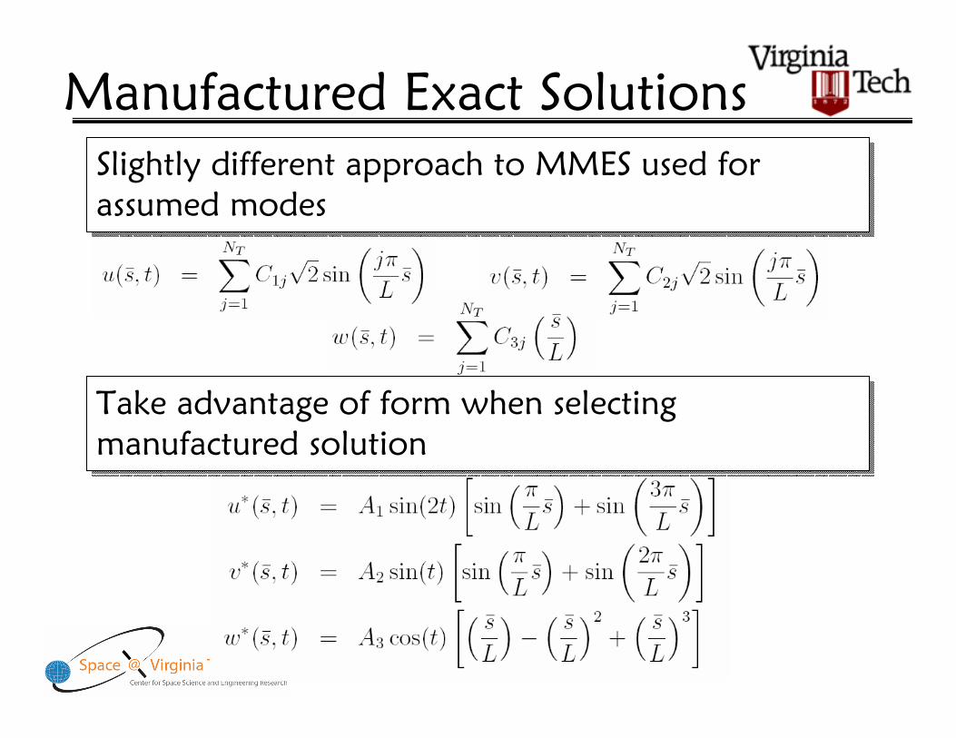
Take advantage of form when selecting
manufactured solution
Take advantage of form when selecting
manufactured solution
Manufactured Exact Solutions
Slightly different approach to MMES used for
assumed modes
Slightly different approach to MMES used for
assumed modes

Manufactured Exact Solutions
Using enough assumed modes should yield “exact”
solution – and it does
Using enough assumed modes should yield “exact”
solution – and it does

Examples of Tether Motion
Three movies illustrating tether motion
Black – FEM, Blue – assumed modes
Motion equations solved using 5 finite elements
and 5 assumed modes (both transverse and
longitudinal) – note differences in solutions
Three movies illustrating tether motion
Black – FEM, Blue – assumed modes
Motion equations solved using 5 finite elements
and 5 assumed modes (both transverse and
longitudinal) – note differences in solutions

Switch to “Simple” Model
• EDT is treated as a point mass
– Equations of motion are simple
• Magnetic field is assumed to be a
tilted dipole
– Set up and solve minimum
time optimal control problem
with tether direction as the
control

Coordinate Systems
2
2n
1n
3n
3o
1o
2o
1om1
2o
1o
TLi
ψ)ˆˆ(ˆˆ131
nmoo ××=
132ˆˆˆ ooo ×=
||ˆ
3B
Bo
=
We assume the tether is
always in the plane
so that the EDT can
generate the maximum
amount of force.
21ˆˆ oo −

Equations of Motion
z
y
x
vz
vy
vx
=
=
=
m
fz
rv
m
fy
rv
m
fx
rv
zz
y
y
xx
+−=
+−=
+−=
3
3
3
µ
µ
µ
Begin with 6 first-order Two-Body Problem
Equations of Motion:

Equations of Motion
Force is perpendicular to magnetic field and is
expressed in inertial frame.

Equations of Motion
Hamiltonian for optimal control law:
0=
+++++= zvzyvyxvxzyx vvvzyxH λλλλλλ

Equations of Motion
Six equations for the Lagrange costates:

Two-Dimensional Results
EDT Trajectory Constant Thrust
Note: All quantities are nonNote: All quantities are nonNote: All quantities are nonNote: All quantities are non----
dimensionalizeddimensionalizeddimensionalizeddimensionalized
•The EDT reaches target orbit faster than a constant thrust
spacecraft
•True for all comparisons with the same initial conditions
[2]

Two-Dimensional Results
• Near-invariance in costate initial conditions and
time of flight when thrust and phase angle are
increased by same order of magnitude
– Families of solutions can be formed
– Near-invariance breaks down for high thrust and phase
angles

Three-Dimensional Solutions
• The range of inclination angles studied is 0-7.5º.
• Difficulties stem from extreme sensitivity of initial
costates as inclination angle increases.

Three-Dimensional Solutions
• The control angles for maneuvers in different
orbit planes have the same pattern except for one
difference…
Between i = 2º and 3º, EDT rotates in opposite direction at t ≈1.4 TU, but control angles are essentially identical.

• High-fidelity model of electrodynamic tether systems– First-principles derivation of equations of motion
– Two discretization methods
– Manufactured solutions verify numerical methods
• Simplified model used to obtain time-optimal orbit transfer trajectories
• Next steps: characterize domains within which simplified models match high-fidelity model results
• Contact: Christopher Hall [email protected]@[email protected]@vt.edu
Summary

Some Backup Slides

• From MMES results we know that codes for
assumed modes and FEM accurately solve
governing PDEs
• Is one solution method “better” than the other –
does one method converge to exact solution
faster?
• Use Richardson Extrapolation to answer this
question
• From MMES results we know that codes for
assumed modes and FEM accurately solve
governing PDEs
• Is one solution method “better” than the other –
does one method converge to exact solution
faster?
• Use Richardson Extrapolation to answer this
question
Richardson Extrapolation

Use two solutions to extrapolate exact solutionUse two solutions to extrapolate exact solution
Richardson Extrapolation
Use extrapolated solution to estimate how “close” solution
is to the exact solution
Use extrapolated solution to estimate how “close” solution
is to the exact solution
Cannot extrapolate tether displacements – must use a scalar
quantity like length or tension at the end bodies to measure
“closeness” to exact solution
Cannot extrapolate tether displacements – must use a scalar
quantity like length or tension at the end bodies to measure
“closeness” to exact solution
Richardson Extrapolation –
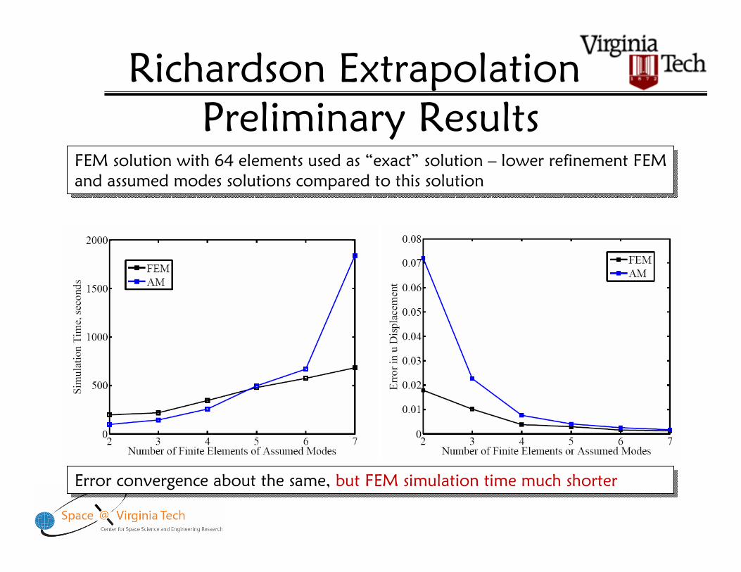
Preliminary ResultsFEM solution with 64 elements used as “exact” solution – lower refinement FEM
and assumed modes solutions compared to this solution
FEM solution with 64 elements used as “exact” solution – lower refinement FEM
and assumed modes solutions compared to this solution
Error convergence about the same, but FEM simulation time much shorterError convergence about the same, but FEM simulation time much shorter

Solution Algorithm
Simulated annealing narrows search field to
identify potential global minima:Simulated annealing
emulates the metallurgical
process for minimizing the
internal energy in the
metal. The “energy state”
is lowered slowly so that
generated test points can
escape local minima and
lead to possible global
minima.
T1
T2
T3
Global Minima