Dynamic behavior of a tensegrity system subjected to ... · PDF fileDynamic behavior of a tensegrity system subjected to follower wind loading ... structures subjected to non-symmetrical

Computers and Structures 81 (2003) 2199–2217

www.elsevier.com/locate/compstruc

Dynamic behavior of a tensegrity system subjectedto follower wind loading

Massimiliano Lazzari a, Renato V. Vitaliani a,*, Massimo Majowiecki b,Anna V. Saetta b

a Department of Construction and Transportation, University of Padova, via Marzolo 9, Padova 35131, Italyb Department of Architectural Construction, Tolentini 191, IUAV, Venice 30135, Italy

Received 14 October 2002; accepted 19 June 2003

Abstract

The aim of this paper is to present a possible develop-line for the study of large lightweight roof structures by non-

linear geometric analysis, under the dynamic effects of the turbulent action of the wind, that can be applied into the

classical engineering applications. In particular the paper deals with the study of tensegrity systems, that can be defined

as pattern that results when push (struts) and pull (tendons) have a win–win relationship with each other. The pull is

continuous and the push is discontinuous. The continuous pull is balanced by the discontinuous push producing an

integrity of tension–compression. Static and dynamic analyses of the wind action effects on one example of such

tensegrity system, i.e. the roof over the La Plata stadium, Argentina, have been performed by using the geometrically

non-linear FE procedure named ‘‘Loki’’. The wind loads are simulated as deformation-dependent forces. Both ex-

perimental data and numerical results available from the roof designers, have permitted to control the reliability of the

proposed mathematical model.

� 2003 Elsevier Ltd. All rights reserved.

Keywords: Wind load; Cable-suspended structures; Geometrical non-linearity; Finite element; Dynamic analysis; Follower load

1. Introduction

A structure immersed in a given flow field, e.g. wind

flux, is subjected to aerodynamic forces dependent on

time and the methods of structural dynamic have to be

applied to determine the response of the structure to

such an action (e.g. [1]). Furthermore, the random fea-

tures of wind action make it necessary to apply the

theory of random vibrations. The response depends on

the characteristics associated with both the structure

and the wind.

It is worth noting that wind-tunnel tests together with

studies of the atmospheric winds have become more

necessary in recent years, because modern construction

* Corresponding author. Tel.: +39-4-9827-5622; fax: +39-4-

9827-5604.

E-mail address: [email protected] (R.V. Vitaliani).

0045-7949/$ - see front matter � 2003 Elsevier Ltd. All rights reserv

doi:10.1016/S0045-7949(03)00291-8

is more sensitive to wind action, especially for light-

weight structural typologies.

Structures consisting of cables or membranes may be

more susceptible to wind effects. In particular, cable roof

structures subjected to non-symmetrical loads [2] may

exhibit greater deformations than most other structures.

In double curvature roofs, the load-bearing and stiffen-

ing cables form a network, which is orthogonal in most

cases. Such roofs may pose serious vibration problems,

requiring the provision of additional ties and lubrication

of the cable intersection.

The final application of the paper is the study of

tensegrity systems. Tensegrity structure was firstly con-

ceived by Fuller [3], who defined the notions of tense-

grity as a contraction of tensional and integrity. With

Snelson�s work in 1948 much research work on different

types of tensegrity system has been carried out during

the past 60 years [4].

ed.

mail to: [email protected]

2200 M. Lazzari et al. / Computers and Structures 81 (2003) 2199–2217

Before Motro presented contiguous strut configura-

tion, the essential ideas of the definition of tensegrity

could be summarized as [5]: (i) composed of compres-

sion (struts) and tension (tendons) elements, (ii) struts

discontinuous while cables continuous, (iii) self-stressed

equilibrium. After tensegrity�s definition changed about

the (ii) point as ‘‘pin-jointed’’.

The definition also diverges at whether a cable dome

can be included within tensegrity system or not. Wang

[6] considers that cable domes are an extensive applica-

tion of the tensegrity concept and tensegrity structures

definitions can be change as (i) self-stressed equilibrium

cable networks in which a continuous system of cable

(tendons) are stressed against a discontinuous system of

structures, (ii) composed of tensegrity simplexes.

There is also no consensus on the definition of cable

domes. The main divergence lies in the different view of

whether the boundary compression ring is included in

the cable dome or not.

However, the most successful application of tenseg-

rity system is the cable dome proposed by Geiger for

Summer Olympic at Seoul, Korea in 1986. As an inno-

vative, lightness dome system, it attracts a lot of atten-

tion from engineers and is widely used in large span

structures, such as Rebdird Arena and the Sun Coast

Dome. The largest existing dome––Georgia Dome––

with an elliptical plan, was designed for the Atlanta

Olympic Game in 1996 [7] by M. Levy. The Georgia

dome is the first Hypar-Tensegrity Dome to built where

hyperbolic paraboloid fabric panels are attached to a

cable net that is stiffened by the use of tensegrity prin-

ciples.

The aim of this paper is to present a possible develop-

line for the study of such large roof structures by non-

linear geometric analysis that can be applied into the

classical engineering applications.

It is worth noting that the development of a non-

linear static as well as dynamic analysis is a minimum

requirements from the viewpoint of engineering practice,

since the hypothesis of geometrical non-linear response

are necessary to capture the real mechanical behavior of

the tensegrity structures, indispensable in the design

phase of such a construction. In the cases of standard

constructions, the load parameter about both wind and

snow conditions can be derived from literature (e.g.

basing on national standard, collection of wind tunnel

tests, books, similar constructions in similar place). On

the other end, in the cases of particular construction of a

certain importance (e.g. the roof of stadium), with a

non-classical well know behavior, some more numerical

simulations (static, dynamic, frequency analysis) as well

as tunnel wind investigations (aeroelastic, aerodynamic

model under laminar or turbulent flow) are indispens-

able.

In the present work, the cable suspension structure at

La Plata Stadium in Argentina is analyzed under the

effects of wind, by using the geometrically non-linear

finite element procedure (named ‘‘Loki’’ [8,9]) developed

according to the total Lagrangian formulation. The

wind action is described as follower loading. In partic-

ular, according to the notation introduced by Schwei-

zerhof and Ramm [10], the case of ‘‘body-attached

pressure load’’ is considered, where only the direction

depends on the deformation within each time step.

First a static analysis is carried out to study the re-

sponse of the structure under the self-weight and pre-

stressing loads and with the wind acting in the two main

directions of the roof. Then the free vibration analysis is

carried out and the frequencies of the structure are ana-

lyzed.

Finally a number of analyses are performed in the

time domain, since the considerable displacements in-

volved make it unsuitable to use the frequency analysis

alone. In fact, determining the structure�s response in the

frequency domain calls for the use of several simplifying

hypotheses, i.e. linearity of mechanical behavior, low

turbulence factor, and negligibility of any motion of the

structure. Moreover, the effects of interactions between

the loading process and the response process have to be

considered for such structures.

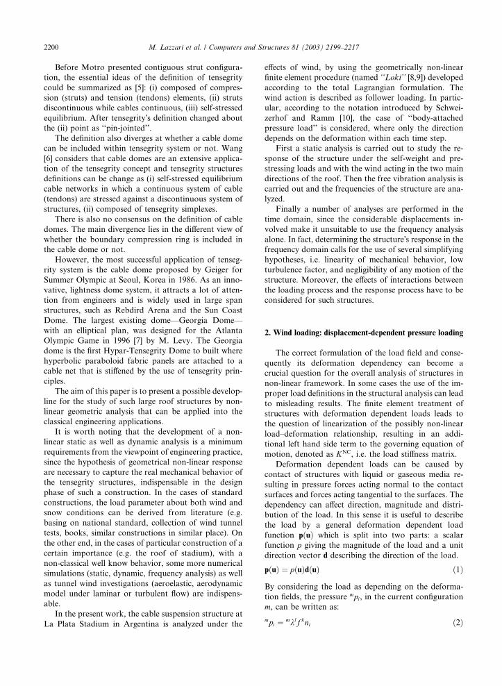
2. Wind loading: displacement-dependent pressure loading

The correct formulation of the load field and conse-

quently its deformation dependency can become a

crucial question for the overall analysis of structures in

non-linear framework. In some cases the use of the im-

proper load definitions in the structural analysis can lead

to misleading results. The finite element treatment of

structures with deformation dependent loads leads to

the question of linearization of the possibly non-linear

load–deformation relationship, resulting in an addi-

tional left hand side term to the governing equation of

motion, denoted as KNC, i.e. the load stiffness matrix.

Deformation dependent loads can be caused by

contact of structures with liquid or gaseous media re-

sulting in pressure forces acting normal to the contact

surfaces and forces acting tangential to the surfaces. The

dependency can affect direction, magnitude and distri-

bution of the load. In this sense it is useful to describe

the load by a general deformation dependent load

function pðuÞ which is split into two parts: a scalar

function p giving the magnitude of the load and a unit

direction vector d describing the direction of the load.

pðuÞ ¼ pðuÞdðuÞ ð1Þ

By considering the load as depending on the deforma-

tion fields, the pressure mpi, in the current configuration

m, can be written as:

mpi ¼ mklf kni ð2Þ

s

r

xm3

2xm1xm

pm

Fig. 2. Element surface loaded in normal direction.

M. Lazzari et al. / Computers and Structures 81 (2003) 2199–2217 2201

where mk is the load multiplier; lf ¼ lf ðlxjÞ represents

the pressure distribution, which depends on the co-

ordinates lxj of the configuration l, where l is the initialconfiguration if l ¼ 0 or the current configuration if

l ¼ m; kni is the unit vector perpendicular to the surface

in the configuration k ¼ 0;m.Different load conditions are related to different

values of the coefficients k and m, i.e.:

• k ¼ 0, l ¼ 0 is the classical case of dead load;

• k ¼ 0, l ¼ m is a case of little practical interest;

• k ¼ m represents the most interesting cases: within

the follower load class we can distinguish the body-

attached load Fig. 1(a), characterized by k ¼ 0 and

l ¼ 0, and the space-attached load Fig. 1(b), charac-

terized by k ¼ 0 and l ¼ m.

Schweizerhof and Ramm [10] have introduced the

notations body-attached load for cases where only the

direction depends on the deformation u (i.e. gas pres-

sure), and space-attached load for cases where addi-

tionally the magnitude of the load and thus its

distribution over the element depends on the deforma-

tion (i.e. hydrostatic pressure).

By considering only the pressure acting on the sur-

face A in the orthogonal direction and assuming the

surface in a configuration m ðmAÞ, the external work of

the pressure mpi is:

mdWext ¼Z

mA

mpi duidma ð3Þ

where ui represents the displacement field.

2.1. Displacement-dependent stiffness

The current loaded surface can be described using a

parametric formulation, in terms of the local normalized

co-ordinates r and s (Fig. 2). The co-ordinates of the

current surface, in configuration 2 and with reference to

configuration 1, can be written as:

2xiðr; sÞ ¼ 1xiðr; sÞ þ uiðr; sÞ ð4Þ

The product of the normal and reference surfaces is

given by 2nid2a ¼ eijkðo2xj=orÞðo2xk=osÞdrds where eijk ¼

Fig. 1. Load defi

0;�1; 1 for an acyclic, cyclic and anticyclic sequence and

the expression of the external virtual work (3) by (4) and

the definition of 2nid2a omitting non-linear term be-

comes:

2dWext ¼ eijk2kZr

Zs

lfolxjor

olxkos

dui drds

þ eijk2kZr

Zs

lfoujor

olxkos

�þ olxj

oroukos

�dui drds

ð5Þ

Since wind load is usually classified as a body-attached

load, only such a case will be considered in the following

analysis.

2.2. Body-attached load

If the load is attached to the body, the load functionlf depends only on the initial co-ordinates, i.e. l ¼ 0:0f ¼ 0f ð0xnÞ (for space-attached load 2f ð2xnÞ ¼ 1fþðo1f =o1xnÞun þ � � �, n ¼ 1; 2; 3). Therefore in the expres-

sion of the external virtual work (5) the first term is

independent of the current displacements and represents

the usual load vector, while the second one 2dWext;L

contains the displacement-dependent effect. Only this

part denoted by L is considered below

2dWext;L ¼ eijk2kZr

Zs

oujor

o1xkos

0f dui

� ��

þ oujos

�� o1xk

or0f dui

��drds ð6Þ

nition [10].


Integration by parts of the load stiffness term leads to:

2dWext;L ¼ �eijk2kZr

Zsuj

o

oro1xkos

0f dui

� ��

þ o

os

�� o1xk

or0f dui

��drds

þ eijk2kZoRujo1xkor

0f dui dr

þ eijk2kZoRujo1xkos

0f dui ds ð7Þ

using the relation o0for ¼ o0f

oxnoxnor ¼ 0

0f;n oxnor , developing the

derivatives term and adding (6) to both side of (7) we

can rewrite the above equation in the following form:

2dWext;L ¼1

2eijk2k

Zr

Zs

0fo1xjor

uiodukos

��þ dui

oukos

�

þ o1xkos

uiodujor

�þ dui

oujor

��drds

þZr

Zs

00f;n

o0xnor

o1xjos

�� o0xn

oso1xjor

�ukduidrds

þZb

0fujo1xkos

duidsþZb

0fo1xjor

ukduidr�

ð8Þ

By matrix notation ½du�T ¼ ½du1 du2 du3�, ½u�T ¼½u1 u2 u3� and recalling that eijk has not zero only for six

components, the (8) leads to:

2dWext;L ¼1

22k

Zr

Zs½du�T½bKKNC;I�½u�drds

�

þZr

Zs½du�T½bKKNC;II�½u�drds

þZb½du�T½bKKNC;III�½u�ds

þZb½du�T½bKKNC;IV�½u�dr

�ð9Þ

where the operator matrix are:

Domain terms:

½bKKNC;I� ¼ 122k0f ð½Dr� � ½Ds�Þ; ½bKKNC;II� ¼ 1

22k½0f � ð10Þ

½Dr� ¼0 1x3;sðro� orÞ 1x2;sðor �r oÞ

1x3;sðor � roÞ 0 1x1;sðro� orÞ1x2;sðro� orÞ 1x1;sðor � roÞ 0

24

35

½Ds� ¼0 1x3;rðso� osÞ 1x2;rðos � soÞ

1x3;rðos � soÞ 0 1x1;rðso� osÞ1x2;rðso� osÞ 1x1;rðos � soÞ 0

264

375

½0f � ¼0

P3

j¼100f;jð0xj;s0x3;r � 0xj;r0x3;sÞ �

P0

PSkew-symmetric

264

Boundary terms:

½bKKNC;III� ¼ 122k0f ½D1�; ½bKKNC;IV� ¼ 1

22k0f ½D2� ð11Þ

½D1� ¼0 �1x3;s þ1x2;s

þ1x3;s 0 �1x1;s�1x2;s þ1x1;s 0

24

35

½D2� ¼0 þ1x3;r �1x2;r

�1x3;r 0 þ1x1;rþ1x2;r �1x1;r 0

24

35

where o1xkos ¼ 1xk;s,

o1xkor ¼ 1xk;r, and duj

oukos �

odujos uk ¼

dujðso� osÞuk , duj oukor �odujor uk ¼ dujðro� orÞuk and ðro�

orÞ ¼ �ðor � roÞ.Within the framework of the finite element approach,

the load stiffness element matrices for body-attached

load are always non-symmetrical in the boundary terms

and in the domain terms for a non-uniform load [10].

It is worth noting that a displacement dependent load

contributes with an un-symmetric component, i.e. the

load stiffness matrix, to the tangent stiffness matrix and

in general it cannot be expressed as f ¼ oV =ou. How-

ever, it cannot be excluded that in same particular cases

a load potential (V) could be defined, even in presence of

a non-uniform load.

3. FEM numerical model

The geometrical non-linear analysis was carried out

using a finite element code, named ‘‘Loki’’, developed

according to the total Lagrangian formulation at the

Department of Structural and Transportation Engi-

neering of the University of Padova. The theoretical

approach based on the total Lagrangian co-ordinate

system offers considerable advantages, because of the

constancy of the initial reference configuration and

therefore the greater simplicity in implementation. The

finite elements in GNL analysis of oriented bodies are

studied considering the oriented body as a continuum,

e.g. [11]. The finite elements employed in the analyses are

isoparametric mono-dimensional (cable and truss) and

bi-dimensional (membrane) elements in R3 space, with

linear or parabolic interpolation function for the geo-

metry and the displacements, e.g. [12–14]. The funda-

mental characteristics of these elements are given below,

while the general references of FEM theory for static

3

j¼100f;jð0xj;s0x2;r � 0xj;r0x2;sÞ

3

j¼100f;jð0xj;s0x1;r � 0xj;r0x1;sÞ

0

375

X3

ζ

φ1 φ6

X1

φ5 ξ'

ξ

φ1

φ''1 φ'2

φ'2φ2 φ7

γ '

φ1φ''2

γ

η X2

X3

X1

X2

X'3

X'2

X'1

η

ζξ''

ζ

3

η '

ζ'ηa/2

ζ(b/2)senφ3φ4

p0

ab

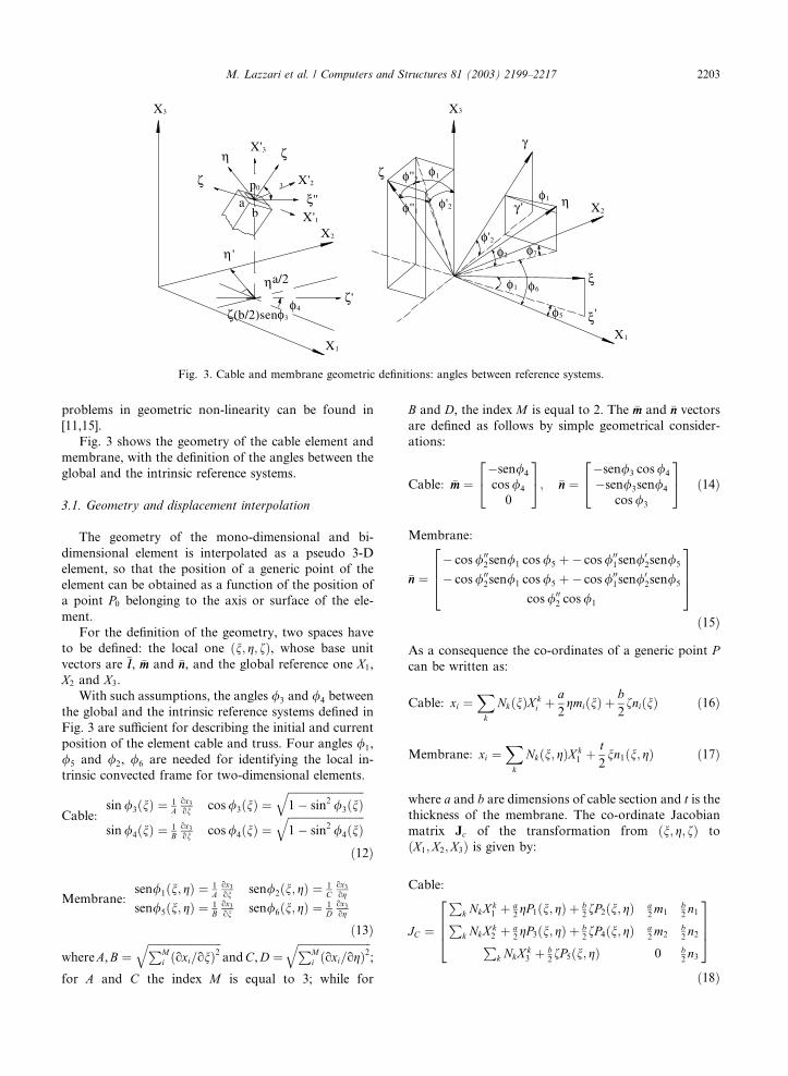
Fig. 3. Cable and membrane geometric definitions: angles between reference systems.


problems in geometric non-linearity can be found in

[11,15].

Fig. 3 shows the geometry of the cable element and

membrane, with the definition of the angles between the

global and the intrinsic reference systems.

3.1. Geometry and displacement interpolation

The geometry of the mono-dimensional and bi-

dimensional element is interpolated as a pseudo 3-D

element, so that the position of a generic point of the

element can be obtained as a function of the position of

a point P0 belonging to the axis or surface of the ele-

ment.

For the definition of the geometry, two spaces have

to be defined: the local one ðn; g; fÞ, whose base unit

vectors are �ll, �mm and �nn, and the global reference one X1,

X2 and X3.

With such assumptions, the angles /3 and /4 between

the global and the intrinsic reference systems defined in

Fig. 3 are sufficient for describing the initial and current

position of the element cable and truss. Four angles /1,

/5 and /2, /6 are needed for identifying the local in-

trinsic convected frame for two-dimensional elements.

Cable:sin/3ðnÞ ¼ 1

Aox3on cos/3ðnÞ ¼

ffiffiffiffiffiffiffiffiffiffiffiffiffiffiffiffiffiffiffiffiffiffiffiffiffiffiffiffi1� sin2 /3ðnÞ

qsin/4ðnÞ ¼ 1

Box3on cos/4ðnÞ ¼

ffiffiffiffiffiffiffiffiffiffiffiffiffiffiffiffiffiffiffiffiffiffiffiffiffiffiffiffi1� sin2 /4ðnÞ

qð12Þ

Membrane:sen/1ðn; gÞ ¼ 1

Aox3on sen/2ðn; gÞ ¼ 1

Cox3og

sen/5ðn; gÞ ¼ 1B

ox3on sen/6ðn; gÞ ¼ 1

Dox3og

ð13Þ

whereA,B ¼ffiffiffiffiffiffiffiffiffiffiffiffiffiffiffiffiffiffiffiffiffiffiffiffiffiffiffiPM

i ðoxi=onÞ2

qandC,D ¼

ffiffiffiffiffiffiffiffiffiffiffiffiffiffiffiffiffiffiffiffiffiffiffiffiffiffiffiPMi ðoxi=ogÞ

2q

;

for A and C the index M is equal to 3; while for

B and D, the index M is equal to 2. The �mm and �nn vectors

are defined as follows by simple geometrical consider-

ations:

Cable: �mm ¼�sen/4

cos/4

0

24

35; �nn ¼

�sen/3 cos/4

�sen/3sen/4

cos/3

24

35 ð14Þ

Membrane:

�nn ¼� cos/00

2sen/1 cos/5 þ� cos/001sen/

02sen/5

� cos/002sen/1 cos/5 þ� cos/00

1sen/02sen/5

cos/002 cos/1

2664

3775

ð15Þ

As a consequence the co-ordinates of a generic point Pcan be written as:

Cable: xi ¼Xk

NkðnÞX ki þ a

2gmiðnÞ þ

b2fniðnÞ ð16Þ

Membrane: xi ¼Xk

Nkðn; gÞX k1 þ t

2nn1ðn; gÞ ð17Þ

where a and b are dimensions of cable section and t is thethickness of the membrane. The co-ordinate Jacobian

matrix Jc of the transformation from ðn; g; fÞ to

ðX1;X2;X3Þ is given by:

Cable:

JC ¼

Pk NkX k

1 þ a2gP1ðn; gÞ þ b

2fP2ðn; gÞ a

2m1

b2n1P

k NkX k2 þ a

2gP3ðn; gÞ þ b

2fP4ðn; gÞ a

2m2

b2n2P

k NkX k3 þ b

2fP5ðn; gÞ 0 b

2n3

2664

3775ð18Þ


Membrane:

JC ¼

PkoNkon X

k1 þ t

2nP1ðn; gÞ

PkoNkon X

k1 þ t

2nP2ðn; gÞ t

2n1P

koNkon X

k2 þ t

2nP3ðn; gÞ

PkoNkon X

k1 þ t

2nP4ðn; gÞ t

2n2P

koNkon X

k3 þ t

2nP5ðn; gÞ

PkoNkon X

k1 þ t

2nP6ðn; gÞ t

2n3

2664

3775

ð19Þ

where Piðn; gÞ are functions obtained by the derivation

of �mm and �nn with respect to n for cable ði ¼ 1–5Þ or by the

derivation of �nn with respect to n and g for membrane

ði ¼ 1–6Þ.Therefore the deformation can be obtained by the

usual relationship e ¼ ðJTJ � IÞ=2.Finally the stresses can be simply evaluated from

their corresponding deformations referred to the in-

trinsic co-ordinate system.

For the case of deformation independent loads, the

tangential stiffness matrix KT is simply derived as de-

rivative of the internal forces with respect to the nodal

displacements, leading to the sum of the elastic ðKEÞ,geometric stiffness ðKLÞ and initial stress ðKSÞ matrices.

In the present case, where the loads depend on the de-

formation, the linearization of the load operator results

in an additional left hand side term, the load stiffness

matrix ðKNCÞ. The global stiffness matrix governing the

non-linear problem is (see e.g. [16,17]):

Fig. 4. Geometry of the roof stru

KT ¼ KE þ KL þ KS � KNC ð20Þ

Large displacements and rotations, but only small

strains, are assumed in the kinematics relations. A

Newmark integration scheme with a full Newton–

Raphson iteration technique has been employed to solve

the non-linear dynamic equation.

4. La Plata stadium

The roof structure of La Plata stadium is defined as

tensegrity system. Fig. 4 shows the geometry of the La

Plata stadium roof, made by the same structural de-

signer of the Georgia Dome [7]. In the following the

description of such a roof is briefly reported (e.g. [18]).

‘‘The plan of the La Plata stadium roof is obtained

from the intersection of two circles with a radius of 85.62

m and centers 48 m apart. Adapting the concept to non-

monotonic hoops entailed introducing an arch across

the pinched waist centerline of the stadium to resist the

outward thrust. Due to the presence of the kink, rigid

rids were required by the arch instead of all cables.

A triangulated perimeter truss resting directly on the

top of the seating berm provides resistance against both

horizontal forces and gravity loads. A triangle steel

trussed compression ring encircles the dome area. It is

cture at La Plata stadium.


about 9 m wide and 13 m high and it sits at the top of

berm that forms the seating bowl for the stadium.

At the top of the compression ring posts, an inner top

chord forms the spring line for the dome, which consists

of the triangulated ridgnet of cables that is characteristic

of the Cable Dome. A series of three tension hoops step

inward and upward from the inner top chord. Radial

cables hold the first of the hoops. Slopping down from

the inner top chord; it supports vertical rigid posts that

connect to the ridgnet. Diagonal cables angle down from

that point to pick up the next tension hoop. The process

repeats itself until the top of the third ring is reached. A

diamond-like array of radial cables springs from the third

ring to form the tent-like cupola of each peek. The cup-

olas permit free air flow thought an opening with a 15-m

diameter in the lower level roof surface of each of two

peaks. A fibber-glass membrane covers the structure.’’

The analysis of structural behaviors of cables dome

involves geometrical configuration finding, determina-

tion of initial stress states and the response evaluation

under the external load. Since the cable dome is a geo-

metrically flexible system, studies of cable domes should

take into account non-linear features and the existence

of an initial stress that gives the structural rigidity.

Such a system is fully three-dimensional and there-

fore benefits from the triangularization of structural

elements, which enable an improvement in its load-

bearing capacity.

The 3-D finite element mesh used in the analyses is

composed of three main sub-structures: (a) the upper

closure elements; (b) the tensegrity system and (c) the

edge space-truss (Fig. 5) [19]. The cable and membrane

isoparametric elements are degenerated 3-D elements,

according to U-linear finite element theory. A synthetic

description of such elements can be found in the above

paragraph and in previous paper of the authors (e.g. [8]).

The 3-D model of the roof includes 1168 one-dimen-

Fig. 5. Finite element model for Loki code.

sional two-node elements (cable and truss) and 285 four-

node membrane elements. The latter are deformed so as

to make two nodes coalesce.

4.1. Static analysis

4.1.1. ‘‘State 0’’

A cable dome needs to be pre-stressed to compensate

the tendency of same cable to go slack. Instead of pre-

stressing with reference to a balanced stress state, the

program was left to seek a balanced configuration. This

balanced configuration implies considerable deforma-

tions of the structure and the reaching of a very different

stress state from the one resulting from the initial pre-

stressing. In this analysis, the deformation of the edge

space-truss structure coincides with a contraction due to

the effect of the compression induced and this contrac-

tion causes a release of the tensegrity system and a

consequent discharge of the stress in the cables and ties

that form the roof. The effect of the contraction is

therefore fundamental to the study of the structure as a

whole. The results are compared with other two finite

element codes used by the designers to perform the static

loading analysis, and the LARSA program used only for

the dynamic mode shape analysis. This program was

been used in the past for the Georgia dome cable roof

structure (e.g. [7]).

Fig. 6 shows the results of the analysis under the self-

weight and pre-stressing loads, in terms of displacement

contours. The maximum values of displacement in X , Yand Z directions obtained by the analysis are respec-

tively: )0.427, )0.250 and )0.526 m corresponding to

the deflection ratios L=400, L=684 and L=323 (where L is

the minimum dimension of the suspended roof, exclud-

ing the space-truss, i.e. 171 m).

It is worth noting the good agreement of the results

obtained by the present analyses with those performed

by the designer of the cable roof: the BLD3D code

provides maximum values of displacement X ¼ �0:434m, Y ¼ �0:249 m and Z ¼ �0:520; the LARSA code

provides max X ¼ �0:447 m, max Y ¼ �0:252 m and

max Z ¼ �0:550. The displacement of the edge space-

truss nodes laying on the X -axis in the X direction

amounts to 5.39 cm, while for the corresponding points

on the Y -axis the displacement is 10.95 cm.

The stress state for the first loading condition is

shown in Fig. 7: it is evident that there is a high force

variation between elements near each other that belong

to the same level. This not homogeneous structural re-

sponse behavior is more evident for the cables that

compose the first and third levels of the structures and

around the intersection zone of the two cables dome,

while the forces in the hoop cables remain relatively

constant in the entire roof. The force in some elements

of the third level is very low if it is compared with other

element. The behavior of the whole structure is function

Fig. 6. Self-weight and pre-stressing loads: displacements [m] along (a) X -direction, (b) Y -direction and (c) Z-direction.

-10000

-8000

-6000

-4000

-2000

0

2000

4000

0 2 4 6 8 10 12 14

For

ce[k

N]

I II˚ III˚-3000

-2000

-1000

0

1000

2000

3000

0 2 4 6 8 10 12 14

For

ce[k

N]

I˚ II˚ III˚

(a) (b) (c)

66

184

Fig. 7. Forces diagram about the up and down cable under pre-stress and dead load.


of the geometrical plan design and in particular the in-

tersection of the two basic shape determine a singular

zone that breaks the regular distribution of the cable�sforces typical for circular or elliptic shape form. Intro-

ducing an arch across the pinched waist centerline of

the stadium, the stiffness and the consequent behavior of

the structures is not uniform for the stress and the

displacement.

4.1.2. Wind load

After the equilibrium shape under pre-stress and

dead load is established, the behavior of the structures is

investigated under static and dynamic wind load. The

static wind load is applied in 10 steps after the config-

uration of equilibrium for pre-stressing and self-weight

has been reached.

The static analysis of the wind�s action is simplified,

dividing the roof into three bands in which the load

acting in the direction normal to the surface takes on

values of 0.50, 1.00 and 0.75 kN/m2. The analysis is

performed for the two main directions of the roof, that is

with the wind acting in the X and Y directions.

The purpose of this analysis is to identify the stress

and strain characteristics to use in relation to the dy-

namic analyses discussed later on. That is why the wind

is assumed to exert an action entirely of depression over

the whole surface of the roof.

The results of wind tunnel tests performed at the

structural dynamics laboratory of the Federal University

of Rio Grande do Sul, in Brazil (UFRGS) demonstrate

that there is always a positive pressure zone, however.

The stress derived from the wind acting in the X di-

rection (Fig. 7(a)) is characterized by the stress being

cancelled in four roof cables (see Fig. 7(b)). The maxi-

mum displacements are 0.459, 0.294 and 0.715 m in the

X , Y and Z directions, respectively, corresponding to the

deflection ratio: 1/373, 1/582 and 1/240.

The wind load in the Y direction (Fig. 9(a)) is heavier

on the structure, setting to zero the stress not only on the

cables considered in the previous situation, but also in

another 4 cables, as shown in Fig. 9(b). In this case the

maximum displacements are 0.307, 0.342 and 0.738 m in

the three directions, respectively, corresponding to the

deflection ratio: 1/557, 1/500 and 1/232. Table 1 reports

the comparison between the Loki response and the

BLD3D response. The obtained results agree with

maximum displacements obtained with other non-linear

geometric code.

Observing the trends of the stresses in Figs. 8 and 9, it

becomes evident that the stress response shows a non-

linear behavior. In fact, the diagrams show that the re-

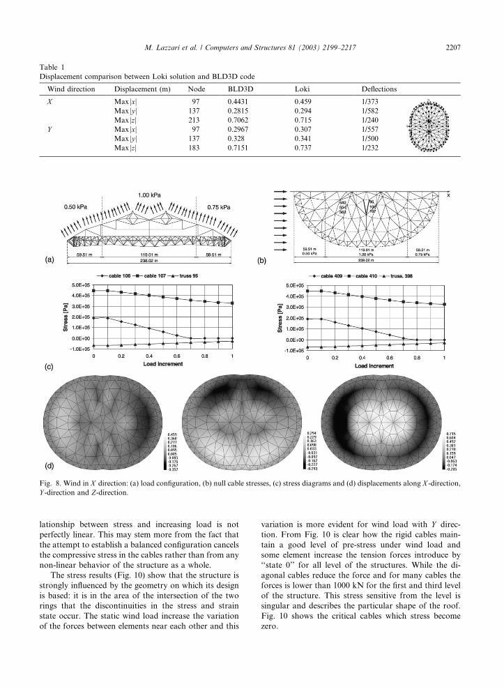
Table 1

Displacement comparison between Loki solution and BLD3D code

Wind direction Displacement (m) Node BLD3D Loki Deflections

X Max jxj 97 0.4431 0.459 1/373

Max jyj 137 0.2815 0.294 1/582

Max jzj 213 0.7062 0.715 1/240

Y Max jxj 97 0.2967 0.307 1/557

Max jyj 137 0.328 0.341 1/500

Max jzj 183 0.7151 0.737 1/232

Fig. 8. Wind in X direction: (a) load configuration, (b) null cable stresses, (c) stress diagrams and (d) displacements along X -direction,Y -direction and Z-direction.


lationship between stress and increasing load is not

perfectly linear. This may stem more from the fact that

the attempt to establish a balanced configuration cancels

the compressive stress in the cables rather than from any

non-linear behavior of the structure as a whole.

The stress results (Fig. 10) show that the structure is

strongly influenced by the geometry on which its design

is based: it is in the area of the intersection of the two

rings that the discontinuities in the stress and strain

state occur. The static wind load increase the variation

of the forces between elements near each other and this

variation is more evident for wind load with Y direc-

tion. From Fig. 10 is clear how the rigid cables main-

tain a good level of pre-stress under wind load and

some element increase the tension forces introduce by

‘‘state 0’’ for all level of the structures. While the di-

agonal cables reduce the force and for many cables the

forces is lower than 1000 kN for the first and third level

of the structure. This stress sensitive from the level is

singular and describes the particular shape of the roof.

Fig. 10 shows the critical cables which stress become

zero.

Fig. 9. Wind in Y direction: (a) load configuration, (b) null cable stresses, (c) stress diagrams and (d) displacements along X -direction,Y -direction and Z-direction.

Fig. 10. Stress diagram about the up and down cable under static wind load: (a) X -direction and (b) Y -direction.



4.2. Dynamic analysis

4.2.1. Natural frequency

The frequencies of the structure were analyzed. Given

the geometrically non-linear nature of the problem, the

calculation is carried out with the stiffness matrix de-

rived from the solution of problem with the pre-stressing

and the self-weight of the structure. The natural fre-

quency was obtained by solving the classic eigenvalue

problem using the total stiffness matrix (20) under

gravity mass matrix ½M �. Fig. 11 shows the modal shapes

of the structure.

The analysis of the frequencies and vibration modes

shows that the structure behaves like an arch, since the

Fig. 11. First to fourth modal shapes of the cable roof.

first and third vibration modes coinciding with the first

two vibration modes along direction X plane YZ and Yplane XZ are antimetric with frequencies of 1.055 and

1.443 Hz. These frequencies are taken for reference in

interpreting the results obtained from the dynamic tests

in the time domain through the evaluation of the power

spectrum. The fundamental period is about T0 ¼ 1 s, and

for the dynamic analyses in the time domain an inte-

gration step of 1/20 of T0, i.e. 0.05 s, is used. The LARSA

code provides 0.949, 1.086, 1.252 and 1.571 Hz. The first

four Georgia Dome�s vibration modes correspond to

frequency of 0.441, 0.682, 0.716 and 0.725 Hz for the pre-

stress and dead load condition. The La Plata stadium is

more rigid then Georgia Dome because the frequency is

about two times Georgia�s frequency. The difference

between the two structures is probably due to the dif-

ferent pre-stress state, the shape of the roofs and the

presence of the up hoop cable for the La Plata Stadium.

The stiffness of the whole structure, considering the very

large dimension of the roof (long span 238 and 187 m), is

not too much low and it is uniformly distributed. The

structure is characterized by principal global stiffness and

the mode and frequency derived from the interaction

between the tensegrity system and the steel ring. The

natural mode of the roof changes if we consider the rigid

ring fix and split the structures in two parts: cable net and

rigid ring. For this reason is fundamental to study the

response of structure as a whole roof.

4.2.2. Wind tunnel investigations

For the purposes of a qualitative comparison, the

following paragraphs outline some of the results of the

experimental study in the wind tunnel on a rigid and a

reduced aero-elastic models of the roof (each con-

structed at 1:400 scale), performed at the structural dy-

namics laboratory of the Federal University of Rio

Grande do Sul, in Brazil (UFRGS).

The rigid model (Fig. 12) was used to ascertain the

pressure coefficients to use for the subsequent assess-

ment of the loads due to wind. Fig. 12 also shows the

pressure points, while Fig. 13 illustrates the signals

measured in the tunnel on two points 23 (black line) and

34 (gray line) in terms of: time histories of the local

external pressure for an incidence angle of 0�, 90�, 180�and 270�; Fourier spectral density; peak, mean and root

mean square (rms) value of the pressure and Cp.

In Fig. 12 we can observe the variation of the pres-

sure time history when the angle changes, and the two

point 23 and 24 from leeward become upwind. The

pressures remain negative pressures and the effect of the

wind under the roof is similar to a depressor load. Near

the ring in correspondence to the principal axes of the

structures the pressure change the value and the sign

when the wind changes the angle between its direction

and the roof axes.

Fig. 13. Signals measured in the wind tunnel (rigid model) [20].

Fig. 12. Wind tunnel experiments: rigid model [20].


The comparison between the times history of the

pressure carried out with reference to the center of the

membrane panel and by pneumatic means of the pres-

sure panel shown that central pressure is lower than

pneumatic pressure for effect of light increase of wind

static load [20].

Fig. 14. Pressure coefficients along (a)

The pressure coefficients are mapped in Fig. 14 and

show that, with a wind acting in directions X and Y ,there is a positive pressure in the zone where the fluid

flux becomes attached to the roof, while for the rest of

the roof there is only a depression. The maximum de-

pression coefficients are found in the two upper domes.

X -direction and (b) Y -direction.

Fig. 15. Wind tunnel experiments: aero-elastic model [21].


In Fig. 14 the absolute coefficients obtained by com-

bining the internal and external Cp coefficients are

mapped.

The second model used in the experimental tests, i.e.

the reduced aero-elastic model (Fig. 15) was tested in the

wind tunnel with a wind coming to bear at 0�, 45� and90� and using increasing velocities, so that the dynamic

pressure was about 1/4, 1/2, 3/4 and the whole of the

maximum pressure obtainable in the tunnel. The me-

chanical characteristics of the reduced aero-elastic

model have been calibrated according to the free vi-

bration modes calculated with the theoretical model

carried out by engineer designer [21]. The element sec-

tion and material used for the aero-elastic model are

chosen to aim the same shapes modes between the the-

oretical global model of the structures and ones of the

theoretical reduce model. The check of the real fre-

quency of the aero-elastic model is carried out by the

free vibration of the model under impulsive load. In this

way the stiffness and damping of the aero-elastic model

is tarred for realistic simulation of the structures.

Fig. 16. Signals measured in the wind

The most important parameter assumed as basic

geometric dimension for reduced aero-elastic model is

the integral length scale (that is a measure of the linear

extent of the gust in wind direction) about 100 m.

The recordings of the changes in deformations and

accelerations are shown in Fig. 16, all for a ¼ 0. The

standard deviation of the fluctuating component, for

both deformation and acceleration, increases with the

increasing test wind speed, bringing the dynamic am-

plification down towards an asymptotic value. Vibration

of the structure is attributed to whirling motion origi-

nating on the edge of the roof or on the external com-

pression ring.

The measure of the dynamic response from the

structure submitted to the fluid–structure iterative effect

depends on the damping and stiffness coefficient matrices

of the structures modified by the iteration matrix, whose

coefficients depend on the wind velocity. The system can

become unstable when the basic matrices become not

positive for effect of the increase wind velocity.

The reduced aero-elastic model allows for the aero-

elastic stability control of the structural system. The

results of the tests carried out by LDEC show the sig-

nificant contribution of the stabilizing effect of the aero-

elastic damping on the lightweight highly deformable

structures response. The structure tested into wind tun-

nel does not show any effect of aero-elastic instability

until the maximum velocity used into the wind tunnel.

4.2.3. Time domain simulation

Non-linear dynamic analysis in the time domain calls

for the generation of a sample temporal set of wind

pressure over the structure. The structure is character-

ized by medium-high level of structural stiffness if we

compare the frequency and static displacement of the

tunnel (aero-elastic model) [21].

nSvðzu2�

Cohð


structures with other large cable roof. For above ob-

servation we can assume in the next simulation the

hypothesis of not interaction between wind force fluc-

tuation and the structures. In this case quasi-static for-

mulation can be assumed so we consider the coefficient

of pressure constant and not function of the structural

motion. By quasi-static theory the simulation of the

wind pressure become the simulation of the wind ve-

locity defined by means of the matrix of the cross-

spectra that describe the stochastic component of the

wind field.

This hypothesis can be considered acceptable because

the structures is characterized by a local high non-linear

geometric behavior but the global stiffness is enough

high that the deformed structures is not far from the

‘‘state 0’’ configuration.

In the next analysis we do not consider the effect of

the internal volume, as a restrain of the structure, be-

cause this effect can be consider not influent for the re-

sponse of the system. The open area around the foot of

the structure, still truss ring, permitted a high exchange

of flow and a consequent low level of internal pressure.

The influence and the importance of the fluid–struc-

ture interaction effects, previously considered by the

authors for membrane roofs showing very large dis-

placement (e.g. [22]) are considered to be not essential

for the response of the actual stiffer structural system.

The aim of the paper, where we want present a possible

develop-line for the study of large roof structures that

can be applied into the classical engineering applica-

tions, included the hypotheses considered acceptable for

the actual case.

Progress in computer performances now allows for

simulation of a significant number of complicated real

phenomena in an accurate and realistic manner. The

generation of artificial samples of random data is a

modern way to deal with uncertainties in variables of

structural behaviors. Furthermore, it represents the

most general approach, given that such numerically

simulated processes must have the same statistical pro-

prieties as the corresponding real quantities [23].

The wind structure at a given pointM , is traditionally

represented by assigning the vectoral temporal law of

speed VðM ; tÞ. In most cases of practical engineering

interest, the lateral and the vertical components of tur-

bulence play a secondary role. In this situation the in-

stantaneous velocity may be described as, e.g. [24]:

VðM ; tÞ ¼ �VVðZÞ þ vðM ; tÞ ð21Þ

where �VVðZÞ is the mean wind speed at height z of pointM of co-ordinates X , Y , Z, which produces static

structural effects only, and fluctuating term vðM ; tÞwhich is the longitudinal component of the zero mean

velocity fluctuation, a random function of space M and

time t, causing a dynamic effect.

In common engineering applications, turbulence is

usually treated as a multidimensional stochastic sta-

tionary Gaussian process, which is characterized, in the

domain of n frequencies, by its cross-correlated power

spectral density SvðM ;M 0; tÞ. The study of this term may

be simplified by assuming that the imaginary component

of the cross-spectrum is negligible for the purposes of

the study that is to be carried out:

SvðX ; Z;X 0; Z 0; nÞ ¼ffiffiffiffiffiffiffiffiffiffiffiffiffiffiffiffiffiffiffiffiffiffiffiffiffiffiffiffiffiffiffiffiSvðZ; nÞSvðZ 0; nÞ

pCohðX ; Z;X 0; Z 0; nÞ

ð22Þ

where SvðZ; nÞ represents the power spectral density

function of along-wind turbulence at height Z and

CohðX ; Z;X 0; Z 0; nÞ represents the coherence function

of longitudinal fluctuations at points MðX ; ZÞ and

M 0ðX 0; Z 0Þ of the plane p orthogonal to the mean wind

direction y.The mathematical model involved is based on the

Akaike–Iwatani algorithm [25,26] with a low level of

regression (ARð3Þ). The data generation is based on the

following stochastic characteristics:

Ground roughness: z0 ¼ 0:2 m;

Reference velocity: v0 ¼ 30 m/s at an elevation of 10 m;

Spectrum:

; nÞ ¼ 2:21b2:5f

ð1þ 3:31b1:5f Þ5=3with b ¼ 5:53

Vinckery�s coherence function:

y; z; y0; z0;nÞ ¼ exp�2n

ffiffiffiffiffiffiffiffiffiffiffiffiffiffiffiffiffiffiffiffiffiffiffiffiffiffiffiffiffiffiffiffiffiffiffiffiffiffiffiffiffiffiffiffiffiffiffiffiffiC2

y ðy� y0Þ2 þC2Zðz� z0Þ2

q�VV ðzÞþ �VV ðz0Þ

0@

1A

where CY ¼ 11:5 and CZ ¼ 11:5 are the decay parame-

ters. The wind is simulated assuming the Vinckery�scoherence for plane orthogonal to wind directions

(cross-wind) whereas the correlation of the signal in the

own direction (along wind direction) is introduced by

adding a delay, s ¼ ½xi=VmðziÞ � xj=VmðzjÞ� in according

with Taylor�s hypothesis. Taylor�s hypothesis states thatthe turbulence is converted downstream unchanged with

the mean velocity [27]. For further details of the algo-

rithm and of how the frequency content of the generated

signal is verified, refer to [9,28].

The mean wind velocity is assumed to have a loga-

rithmic trend. The signal is generated at all the points

above the roof, amounting to a total of 167 nodes (Fig.

4) and the selected signal simulation step is 0.2 s.

The 167 histories generated by the auto-regressive

simulator are the velocity field in which the structure is

immersed. Fig. 17 shows the map of the velocities in

4 instants where Dt ¼ 0:2 s for a wind acting in the X

Fig. 17. Simulated wind velocity [m/s] in X direction at (a) 2 s, (b) 2.2 s, (c) 2.4 s and (d) 2.6 s.

0.0E+00

1.0E+00

2.0E+00

3.0E+00

4.0E+00

5.0E+00

0 10 20 30 40Time [sec]

max

imu

mve

loci

ty[m

/s]

0.0E+00

1.0E+00

2.0E+00

3.0E+00

4.0E+00

5.0E+00

0 10 20 30 40Time [sec]

0.0E+00

5.0E-01

1.0E+00

1.5E+00

2.0E+00

2.5E+00

3.0E+00

0 10 20 30 40Time [sec](a) (b) (c)

Fig. 18. Time histories of maximum structural velocity: (a) Z-direction, (b) X -direction and (c) Y -direction.


direction, illustrating the time-dependent development

of the velocity field over the entire roof.

The corresponding pressure histories are assessed by

means of the pressure coefficients established from the

previously described wind tunnel tests on models de-

scribed in the above paragraph. In the next part of the

paper we refer to dynamic simulation under wind load

with X along wind direction. This direction is parallel to

the principal axes of the structure (Fig. 4). It is worth

noting that the response of the system under other wind

directions are similar to that obtained along X direction.

The dynamic analyses are performed without taking

into account the effect of the relative velocity of the

structure, with reference loading histories. This hy-

pothesis is assumed to be acceptable because the struc-

0.0E+00

5.0E+03

1.0E+04

1.5E+04

2.0E+04

2.5E+04

3.0E+04

0 10 20 30 40Time [sec]

To

talS

trai

nE

ner

gy

c

(a) (b

Fig. 19. Time histories of (a) total stra

ture�s velocity has lowed, as it is possible to observe it in

Fig. 18 were the maximum velocity for the structure in

X , Y and Z directions are shown.

Fig. 19 shows the time history of total strain and

total kinetic energy: the first quantity pass from zero to

the static value after solution of the ‘‘state 0’’, pre-stress

and dead load. It is worth noting that after the initial

step, the dynamic simulation determine a low variation

of the total strain energy. This response illustrates how

the energy variation under wind load action is smaller

than the level reached by pre-stress and dead load con-

dition and the external load do not change the global

behavior of the structure.

The roof is a light structures and the total kinetic

energy is low and non-comparable with total strain

0.0E+00

5.0E+01

1.0E+02

1.5E+02

2.0E+02

2.5E+02

3.0E+02

3.5E+02

4.0E+02

0 10 20 30 40Time [sec]

To

talK

inet

icE

ner

gy

)

in energy and (b) kinetic energy.


energy so the inertial forces are less important of the

elastic forces.

The effect of the structural damping is not evident if

we consider the diagram of the system�s energy and this

is due to the low structural mass of the system and the

correspondent low structural damping.

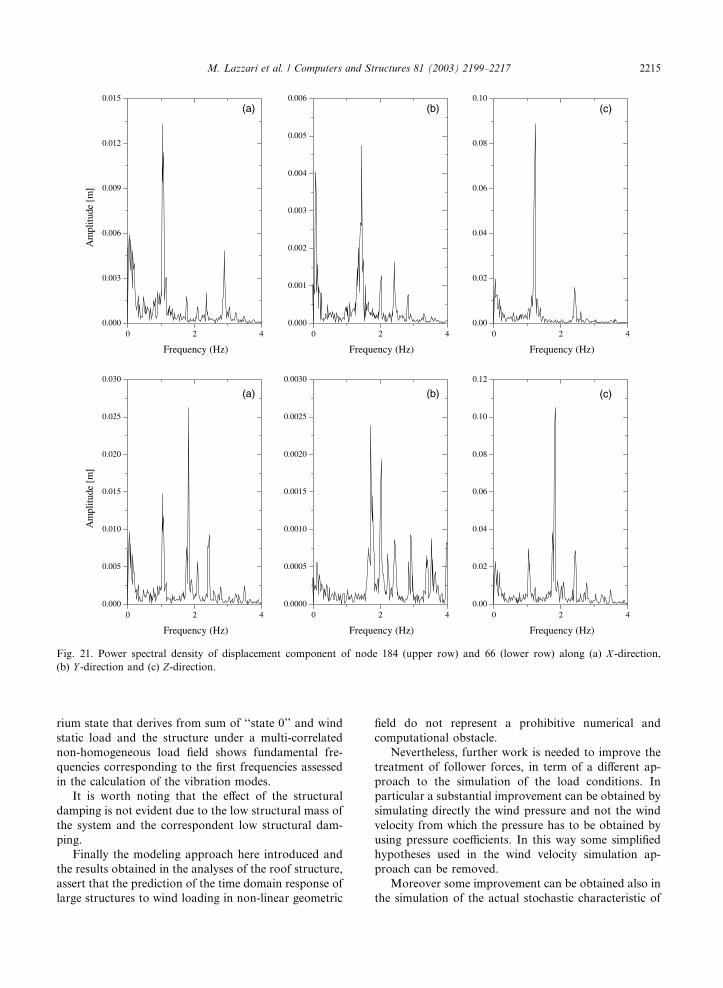
The displacement�s amplitude in X and Y directions

are lesser than Z directions as shown in Fig. 20 for node

184 (central node of the roof, Fig. 7). The vibration is

around the equilibrium state that derives from sum of

‘‘state 0’’ and wind static load. The mean value of Xdirection vibration, about )3 cm, corresponds only to

the static displacement of the central point under wind

load with X direction. The analysis with the power

spectrum of the 184 node displacement (upper row of

Fig. 21) shows that the structure submitted to a multi-

correlated non-homogeneous load field has fundamental

frequencies corresponding to the first frequencies as-

sessed in the calculation of the vibration modes. In the

lower row of the Fig. 21 the response of the 66 node

(belonging to X axis, Fig. 7) is shown, demonstrating

-0.1

-0.08

-0.06

-0.04

-0.02

0

0.02

0.04

0.06

0 5 10 15 20 25 30 35 40Time [sec]

Dis

pla

cem

ent

X[m

]

-0.04

-0.03

-0.02

-0.01

0

0.01

0.02

0.03

0 5 10 15 20 25 30 35 40Time [sec]

Dis

pla

cem

ent

Y[m

]

0

0.1

0.2

0.3

0.4

0.5

0.6

0.7

0.8

0 5 10 15 20 25 30 35 40Time [sec]

Dis

pla

cem

ent

Z[m

]

(a)

(b)

(c)

Fig. 20. History of displacements of node 184 along (a) X -direction, (b) Y -direction and (c) Z-direction.

how the principal frequency of the response are the

frequency of antimetric mode of the roof.

The dynamic response of the hoop cable is charac-

terized by a low vibration around the stress imposed by

‘‘state 0’’, that is a typical response of this kind of

structure, and it agrees with static analysis. Instead the

diagonal cable is strongly linked with the external load

and the histories of the stresses, Fig. 22 reflects the be-

havior observed in the static analysis, with the stress in

the some cables frequently becoming zero, characteriz-

ing the critical behavior of the structures. The influence

of the external load is less important for the rigid cable

(Fig. 22(c)) where it is evident that the effect of the wind

load does not change too much the mean stress obtain

by ‘‘state 0’’. The reason of this particular behavior is

due to the type of the external load that is a depressive

load.

5. Conclusion and discussion

The study of lightweight structures used for wide-

span sub-horizontal roofing requires some aspects to be

taken into account. In particular a minimum require-

ments is the development of non-linear analyses both in

static and in dynamic field, the need of an accurate wind

load definition, with the description of the wind�s actionas a force depending on the deformation, and the

availability of reliable numerical procedure to deal with

such constructions.

Up till now the support of wind tunnel investigations

is necessary when dealing with the design phase of

construction for which dynamic and aeroelastic effects

are difficult to predict, like valuable tensegrity systems.

In this paper the structural response of one of such

system, the La Plata Stadium roof, has been carried out

by using static, frequency and dynamic analyses. Con-

cerning the static analysis of ’’state 0 condition’’, a good

agreement of the results obtained by the present analyses

with those performed by the designer of the cable roof is

evidenced. Similarly the static analysis of wind loading

condition produce results which agree with maximum

displacements obtained with other non-linear geometric

code.

Then the dynamic behaviour in term of frequency

analysis of the La Plata roof is compared with that

obtained for other tensegrity structure (i.e. Georgia

Dome) and some considerations have been carried out.

Finally the non-linear dynamic analyses of the roof

have been carried out in the time domain, by assuming

that there is no interaction between wind force fluctua-

tion and the structure. The dynamic response of the roof

reflects the results obtained in the static and frequency

analyses, demonstrating that such a construction does

not show resonance as well as instability phenomena. In

particular the obtained vibration is around the equilib-

0 2 40.000

0.003

0.006

0.009

0.012

0.015

0 2 40.000

0.001

0.002

0.003

0.004

0.005

0.006

0 2 40.00

0.02

0.04

0.06

0.08

0.10

Frequency (Hz)

Am

plitu

de[m

]

Frequency (Hz) Frequency (Hz)

0 2 40.000

0.005

0.010

0.015

0.020

0.025

0.030

0 2 40.0000

0.0005

0.0010

0.0015

0.0020

0.0025

0.0030

0 2 40.00

0.02

0.04

0.06

0.08

0.10

0.12

Frequency (Hz)

Am

plitu

de[m

]

Frequency (Hz) Frequency (Hz)

(a) (b) (c)

(a) (b) (c)

Fig. 21. Power spectral density of displacement component of node 184 (upper row) and 66 (lower row) along (a) X -direction,(b) Y -direction and (c) Z-direction.


rium state that derives from sum of ‘‘state 0’’ and wind

static load and the structure under a multi-correlated

non-homogeneous load field shows fundamental fre-

quencies corresponding to the first frequencies assessed

in the calculation of the vibration modes.

It is worth noting that the effect of the structural

damping is not evident due to the low structural mass of

the system and the correspondent low structural dam-

ping.

Finally the modeling approach here introduced and

the results obtained in the analyses of the roof structure,

assert that the prediction of the time domain response of

large structures to wind loading in non-linear geometric

field do not represent a prohibitive numerical and

computational obstacle.

Nevertheless, further work is needed to improve the

treatment of follower forces, in term of a different ap-

proach to the simulation of the load conditions. In

particular a substantial improvement can be obtained by

simulating directly the wind pressure and not the wind

velocity from which the pressure has to be obtained by

using pressure coefficients. In this way some simplified

hypotheses used in the wind velocity simulation ap-

proach can be removed.

Moreover some improvement can be obtained also in

the simulation of the actual stochastic characteristic of

0.0E+00

1.0E+05

2.0E+05

3.0E+05

4.0E+05

5.0E+05

0 5 10 15 20 25 30 35 40Time [sec]

Str

ess

[Pa]

0.0E+00

1.0E+05

2.0E+05

3.0E+05

4.0E+05

5.0E+05

6.0E+05

0 5 10 15 20 25 30 35 40

Time [sec]

Str

ess

[Pa]

-8.0E+04

-7.0E+04

-6.0E+04

-5.0E+04

-4.0E+04

-3.0E+04

-2.0E+04

-1.0E+04

0.0E+00

0 5 10 15 20 25 30 35 40

Time [sec]

Str

ess

[Pa]

(a)

(b)

(c)

Fig. 22. History of stresses of (a) cable 106, (b) cable 107 and

(c) truss 95.


wind action, which in the case of sub-horizontal

structures may differ significantly from the Gaussian

form.

References

[1] Simiu E, Scanlan R. Wind effects on structures. An

introduction to wind engineering. John Wiley & Sons;

1996.

[2] Christiano P, Seeley GR, Stefan H. Transient wind loads

on circular concave cable roof. J Struc Div ASCE

1974;100(ST11):2323–41.

[3] Fuller RB. Synergetics explorations in the geometry of

thinking. London: Collier Macmillan Publishers; 1975.

[4] Yuan XF, Dong SL. Nonlinear analysis and optimum

design of cable domes. Engng Struct 2002;24:965–77.

[5] Motro R. Tensegrity system: the state of the art. Int J

Space Struct 1992;7(2):75–83.

[6] Wang BB. Cable-strut systems: Part I––tensegrity. J

Construct Steel Res 1998;3:281–9.

[7] Castro G, Levy MP. Analysis of the Georgia Dome Cable

Roof. In: Proceedings of the Eighth Conference of Com-

puting in Civil Engineering and Geographic Information

Systems Symposium, ASCE, Dallas, TX, June 7–9,

1992.

[8] Lazzari M. Geometrically Non-Linear Structures Sub-

jected To Wind Actions, PhD thesis, University of Padua,

2002.

[9] Lazzari M, Saetta A, Vitaliani R. Non-linear dynamic

analysis of cable-suspended structures subjected to wind

actions. Comput Struct 2001;79/9:953–69.

[10] Schweizerhof K, Ramm E. Displacement dependent pres-

sure loads in nonlinear finite element analyses. Comput

Struct 1984;18(6):1099–114.

[11] Zienkiewicz OC, Taylor RL. The finite element method,

McGraw-Hill, vol. I., 1989; vol. II, 1991.

[12] Schrefler BA, Wood RD, Odorizzi S. A total Lagran-

gian geometrically non-linear analysis of combined

beam and cable structures. Comput Struct 1983;17(1):

115–27.

[13] Bolzon G, Schrefler BA, Vitaliani R. Finite element

analysis of rubber membranes, in: Kr€aatzig WB, O~nnate E,

editors. Computational Mechanics of Nonlinear Response

of Shell, 1990. p. 348–77.

[14] Wood RD, Zienkiewicz OC. Geometrically non-linear

finite element analysis of beam, frames, arches and axi-

symmetric shells. Comput Struct 1977;7:725–35.

[15] Bathe K-J. Finite element procedures in engineering

analysis. Englewood Cliffs, NJ: Prentice-Hall Inc.; 1996.

[16] Vitaliani RV, Gasparini AM, Saetta AV. Finite element

solution of the stability problem for nonlinear undamped

and damped systems under nonconservative loading. Int J

Solids Struct 1997;34(19):2497–516.

[17] Mok DP, Wall WA, Bischoff M, Ramm E. Algorithmic

aspects of deformation dependent loads in non-linear static

finite element analysis. Engng Comput 1999;16(5):601–

18.

[18] Weidlinger Associates, http://www.wai.com/Structures/

Fabric/laplata.html.

[19] Lazzari M, Majowiecki M, Saetta A, Vitaliani R. Analisi

dinamica non lineare di sistemi strutturali leggeri sub-

orizzontali soggetti all�azione del vento: lo stadio di La

Plata, 5� Convegno Nazionale di Ingegneria del Vento,

ANIV IN-VENTO-98, 1998 [in Italian].

[20] LDEC (Laboratorio de Dinamica Estrutural e Confiabi-

lidade) 1/1997, UFRGS (Universiade Federal DO Rio

Grande Do Sul).

[21] LDEC (Laboratorio de Dinamica Estrutural e Confiabi-

lidade) 2/1997, UFRGS (Universiade Federal DO Rio

Grande Do Sul).

[22] Lazzari M, Majowiecki M, Saetta A, Vitaliani FE.

Analysis of Montreal Stadium Roof Under Variable

Loading Conditions, Towards a Better Built Environ-

ment––Innovation, Sustainability, Information Technol-

ogy, IABSE Symposium, Australia, September 11–13,

2002.

[23] Borri C, Zahlten W. Fully simulated non linear analysis of

large structures subjected to turbulent artificial wind. Mech

Struct Mach 1991;19(2):213–50.

[24] Solari G. Turbulence modeling for gust loading. J Struct

Engng ASCE 1987;113(7):1550–69.

http://www.wai.com/Structures/Fabric/laplata.html

http://www.wai.com/Structures/Fabric/laplata.html


[25] Iwatani Y. Simulation of multidimensional wind fluctua-

tions having any arbitrary power spectra and cross-spectra.

J Wind Engrg 1982;11:5–18.

[26] Augusti G, Borri C, Gesella V. Simulation of wind loading

and response of geometrically non-linear structures with

particolar reference to large antennas. Struct Safety

1990;8:161–79.

[27] Scruton C. An introduction to wind effects on structures.

Oxford University Press; 1990.

[28] Lazzari M, Majowiecki M, Saetta A, Vitaliani R. Gener-

azione artificiale dell�azione del vento: analisi comparativa

degli algoritmi di simulazione nel dominio del tempo, 5�Convegno Nazionale di Ingegneria del Vento, ANIV IN-

VENTO-98, 1998 [in Italian].

Documents

Dynamic behavior of a tensegrity system subjected to ... · PDF fileDynamic behavior of a tensegrity system subjected to follower wind loading ... structures subjected to non-symmetrical