DYNAMIC ANALYSIS OF FINITELY STRETCHED … ANALYSIS OF FINITELY STRETCHED AND ROTATED THREE-DIMENSIONAL ... dynamic analysis of finitely stretched and ... which remains a smooth space-curve

Compurers d Stnrcrures Vol. 29, No. 5, pp. 875-889, 1988 Printed in Great Britain.

lxl45-7949/88 $3.00 + 0.00 Pcrgamon Press pk

DYNAMIC ANALYSIS OF FINITELY STRETCHED AND ROTATED THREE-DIMENSIONAL

SPACE-CURVED BEAMS

M. IURA and S. N. ATLURI Center for the Advancement of Computational Mechanics, Georgia Institute of Technology,

Mail Code 0356, Atlanta, GA 30332, U.S.A.

(Received 3 September 1987)

Abstract-The problem of transient dynamics of highly flexible three-dimensional space-curved beams, undergoing large rotations and stretches, is treated. The case of conservative force loading, which may also lead to configuration-dependent moments on the beam, is considered. Using the three parameters associated with a conformal rotation vector representation of finite rotations, a well-defined Hamilton functional is established for the flexible beam undergoing finite rotations and stretches. This is shown to lead to a symmetric tangent stiffness matrix at all times. In the present total Langrangian description of motion, the mass-matrix of a finite element depends linearly on the linear accelerations, but nonlinearly on the rotation parameters and attendant accelerations; the stiffness matrix depends nonlinearly on the deformation; and an ‘apparent’ damping matrix depends nonlinearly on the rotations and attendant velocities. A Newmark time-integration scheme is used to integrate the semi-discrete finite element equations in time. Several examples of transient dynamic response of highly flexible beam-like structures, including those in free flight, are presented to illustrate the validity of the theoretical methodology developed in this paper.

1. INTRODUCTION

This paper is concerned with the large defo~ation dynamic analysis of finitely stretched and rotated three-dimensional elastic space-curved beams, ex- tending model developed by Iura and Atluri[l] for such problems, in the static case.

The model used is based on Timoshenko’s hypotheses; the effects of stretching, bending, torsion and transverse shear are taken into account. For sim- plicity, however, the cross-sectional warping effects are neglected. These kinematic assumptions have been employed also by Antman and Jordan [2], Reissner [3] and Simo and Vu-Quoc [4] to develop a thr~-dimensional beam theory. In these references, the existence of prescribed external moments has been postulated a priori. Iura and Atluri [I] have utilized the variational method to derive the consistent boundary conditions in which the external moments arise as a consequence of the applied external forces. Iura and Atluri [l] have observed that the conservative moments (using the definition of Schweizerhof and Ramm [S] as to whether the load is conservative or not) are generally configuration dependent. Argyris et al. [6] have employed the same definition for external moments. Using the rotational degrees of freedom referred to fixed axes of a global Cartesian system, Argyris et al. [6] have derived a nonsymmetric tangent stiffness matrix at the element level. Simo and Vu-Quoc [4] have concluded that, in the context of a classical formulation of rotations, the tangent stiffness matrix becomes symmetric only at

an equilibrium configuration, provided that no distributed external moments are assumed to exist. Iura and Atluri [i], on the other hand, have shown that the use of any three independent components of the finite rotation tensor, as rotational variables, leads to a symmetric tangent stiffness matrix, not only at the equilibrium but also the nonequilibrium configuration, even if the distributed external moments exist in the problem.

The large deformation dynamics of a continuum body have, in the past, been formulated with the use of the total Lagrangian formulation, the updated Lagrangian formulation, the Eulerian formulation, the Euler-Lagrangian formulation and the moving coordinate formulation [7-lo]. Among these formulations, the inertia effects are readily taken into account in the total Lagrangian formulation. Here, therefore, we employ the total Lagrangian formulation and show the capability of the present formulation to simulate the dynamic behavior of finitely stretched and rotated beams.

In this paper the elasto-static model for finitely stretched and rotated space-curved beams, developed by Iura and Atluri [1], is extended to the case of dynamic analysis. In Sec. 2 we summarize the kinematic relations of the present model briefly. The principle of virtual work for elastodynamics is introduced, in Sec. 3, to derive the linear momentum balance (LMB) and angular momentum balance (AMB) conditions and the associated boundary conditions. Depending on the form of virtual variations of the rotational parameters considered, the LMB

876 M. IURA and S. N. ATLURI

and AMB conditions take on different but equivalent forms, as in the static problem. A well-defined functional for Hamilton’s principle is obtained by using one form of rotation parameters, or the components of the finite rotation tensor.

In Sec. 4, the finite element formulation is utilized for deriving the semi-discrete equations of motion. The rotation variables used herein are taken as the Lagrangian components of conformal rotation vector [ll]. Without using the four quarternion or Euler parameters, the singularity, associated with the finite rotation vector, can be avoided with a simple manipulation. As shown in the existing literature [lo, 121, the resulting mass matrix is no longer constant due to the effects of finite rotations. Even though no external damping effects are accounted for in the formulation, the nonlinear terms of the velocity of rotational components appear in the semi-discrete equations.

A variety of time integration schemes has been proposed by many investigators [13]. In this paper, we use the Newmark algorithm to integrate the resulting semi-discrete equations. Although the stability and convergence conditions for the nonlinear dynamic problems have not been established yet, the Newmark family of algorithms has received wide attention.

To demonstrate the validity and the applicability of the present beam theory, numerical examples are presented in Sec. 5. After we confirm the accuracy of the beam model developed herein, we investigate the configuration dependency of the external moments in both planar and nonplanar problems.

2. PRELIMINARIES

2.1. Fundamental hypotheses

The fundamental hypotheses used are itemized as follows:

(1)’ The plane cross-sections of the beam remain plane and do not undergo any change of shape during the deformation.

(2) The cross-sections are constant along the beam axis, which remains a smooth space-curve throughout the deformation.

It should be noted that no simplification is made in the present formulation; not only the rotatory inertia but also the Coriolis and the centrifugal effects are accounted for.

Throughout this paper, the summation convention is adopted; and the Latin indices will have the range 1, 2 and 3, and the Greek indices the range 1 and 2.

2.2. The geometry of the undeformed and deformed beam

We summarize, for completeness, the kinematic relations of the present beam model developed by Iura and Atluri [l].

Let Y” be a convected orthogonal curvilinear coordinate system. The coordinates Y” are taken in the cross-section, while the coordinate Y3 is taken along the beam axis, as shown in Fig. 1. The undeformed base vectors at an arbitrary point in a cross-section of the beam are given, in terms of the undeformed unit base vectors E, at the beam axis, by

A, = E,, (la)

A, = - Y2K3E, + Y’K,E, +g,,E,, (lb)

where

g,= 1 - Y’K2+ Y’K,.

The quantities K, are the components of initial curvature, and the K3 is the initial twist, satisfying the following relations:

E,,,,=KxE,,,, K=K,,,E,,,, @a, b)

where ( ), 3 = d( )/dL where L is the parameter of the length of an arc along the line of origin of the coordinate system Y”, in the reference configuration.

Let e, be the maps of the base vectors E,,, after a purely rigid rotation, denoted by the finite rotation tensor R, alone: that is, e, = RE,,,. In general, due to the shear deformation, the unit vector tangential to the deformed beam-axis does not coincide with the vector e3. From the definition of covariant base vectors, the deformed unit tangent vector, denoted by e,, may be written as:

~3=~mI13E,n, (34

~“II3=@;+u”l,)/& (3b)

g =J[(u’13)2+(~213)2+(1 +u313)21, (3c)

where u( =u”‘E,,,) is the displacement vector at the beam axis, S; the Kronecker delta, and ( ) I 3 denotes a covariant differentiation by using the metric tensor E,= E,.E,.

According to the hypothesis (l), the displacement vector at an arbitrary material point is represented as

U=u+ Y’(e,-E,). (4)

The deformed base vectors at an arbitrary point in a cross-section of the beam are given as

a, = e,,

a3 = (g sin /I, - Y2k3)e,

+(g sinP2+ Y’k,)e,

+ (g/I3 - Y’k, + Y2k,)e3

(5a)

(5b)

Analysis of three-dimensional space-curved beams 877

where

Before the /

After the defor -mation

Fig. 1. Kinematic scheme for highly flexible space-beam analysis.

sin B, = (R.E,).(a” II 3&,,),

tensor, F the deformation gradient tensor, ( )r a transpose, and dA = d Y’ dY2. The components of T

(6a) and M are given by

(6b) T=T”‘e,,,, M=M”e,,,, Pa, b)

(6~) T”= t3mg,,dA, M’= t33Y2g,,dA 6% 4

in which Q is the permutation symbol. The parameters /?, denote the angles of shear deformations. The vector k, defined by k = k,e,,,, satisfies the following differential relation:

(94

e,,,=k xe,. (7) M’ =

J (t” Y’ - t’l Y2)g0 dA, (90

2.3. Strain-stress relationships where tm are the stress tensors defined by According to Atluri [14], the stress resultants and

moments are defined as tmR = sq’q .e 1 j I* (10)

T = s

gOA3.(S, .FT) dA, (84 The (-) in the contravariant tensor components is used to emphasize that these are not components in the convected coordinates Ym. The conjugate strain

M = s

Y”e, x [g,A’.(S,.F’)]dA, (8b) tensors y,,,x are expressed as

Ynu? = a;e, - A;E,,. (11) where A” is the reciprocal basis of A,,,, S, (= ST A, A,) is the second Piola-Kirchhoff stress For one-dimensional beams, we assume that the


following constitutive relationships hold:

t3” = Gy,, , t3’ = &J,~, (1% b)

where G is the shearing modulus and E the Young modulus. Substituting eqns (11) and (12) into eqns (9) and utilizing eqns (5) leads to

T’ GA, T2

T’ Ml =

M2

M3

where

h, = g sin &, h3 = gB3 - l/u,

A = i

g,,dA, A,,= kA,

I- P

(EVW), defined as [ 161

EVW=SP~.6UdV+SP,.~ods,

+ [j-P/6” dS,l::L, (16)

&

0 0 0

GA, 0 0

EA EI,

EI,, Sym.

0 - Cl,

0 Cl2

-Er, 0

-EZ,, 0

EI22 0

GJ

h h2

h, (13)

(1% b)

(14~9 d)

I,= Y”g,,dA, Z,,= Y’Y*g,dA, J J

(1% f)

II, = ( Y2)2g,, dA, I,, = (Y’)‘g dA, 5 5

(Ws h)

where Pb is the vector of body force defined per unit volume of the undeformed beam, denoted as V; PC the vector of distributed surface traction defined per unit area of the undeformed cylindrical surface of the beam, denoted as SC; and P, the vector of distributed surface tractions at the end cross-sections denoted as S,. The quantity I is the length of the beam axis before the deformation, and S, is a part of boundary on which mechanical boundary conditions are prescribed. Since we are concerned with a conservative system of forces, the external forces are expressed as

J= 5

pg,dA, p =(Y’)2+(Y2)2, (14ij)

1; = ki - K, (1W

Pb = PXE,, PC = PiEi, P, = P:E,. (17a-c)

Introducing eqns (17) into eqn (16) yields

The factor k is the shear-correction factor [15]. The strain-energy function per unit length along

the beam axis is obtained as

Ws=;GA,(h,)2+fGA,(h2)2+fEA(h3)2 where

+fEI,,(&)2+f EZr,(&)2 +f GJ$d2 q = q’E,, 4 = $E,, (1% b)

+ EZ, h& - E12h3c2 - EI,,&L2

- GZ,h,E3 + G12h2E3. (15)

It should be emphasized that the widely accepted strain-energy function, expressed by eqn (15), is based on the constitutive eqns (12a, b). If we introduce the well-known constitutive equations such that S3a= Ge3a and S:3 = Ee where e,,,,, denotes the dreen strain tensor, the i&rlting strain-energy function is substantially different from the present one.

2.4. Dejinition of external moments

m = m,e, x E,, fi = Rtije, x E,, (19c, d)

&=IP&dA +~P:IS,,xSlld.r, (19e)

qj= P!dS,, I

(19f)

mmj= Y’Pjg,dA + Y’P!lS,, x S,ld.s, (19g) s s

A,= YdP;dS,, s

(19h)

Argyris et al. [6] have defined a conservative moment as a moment generated by a couple of two equal and opposite conservative forces acting on a rigid lever. In this paper, the definition of the external moments are obtained from the external virtual work

in which S is the position vector at the undeformed cylindrical surface, and ( ),, denotes a differentiation with respect to the coordinate S taken along the bounding curve of the cross-sections. The vector


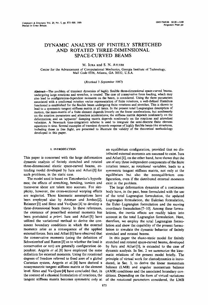
(al P

-4 -3 ‘2+ a 0 _ I. -- Y3

I 1 E -1 I

Before the deformation

(b)

E E -2 w -*.

P2 \

E @b : -1

4 /p

% Y3

After the deformation

Fig. 2. Configuration dependency of prescribed external

S+ is the rotational variation and defined by SI# x Z = 6R+ Rr [14] where I is an identity tensor.

It follows from eqns (19c, d) that the external moments m and iir defined herein are dependent on the deformation. Figures 2(a) and (b) show the configuration dependency of the external moments. Before the deformation, as shown in Fig. 2(a), the equivalent load at point 0 (or the origin of the coordinates Y”) is the force f( = 1 P 1 E,) only. After the deformation, as shown in Fig. 2(b), the equivalent loads at point 0 are not only the forcef( = 1 P ) E,) but also the moment m( = (PIE, x ae,). This example indicates that the external moments are dependent on the deformation.

Argyris et al. [6] have also pointed out the configuration dependency of external moments. They have derived a nonsymmetric tangent stiffness matrix by using the rotational degrees of freedom referred to fixed axis of a global Cartesian system. In this paper, however, the resulting tangent stiffness matrix is always symmetric, as shown later, as long as any three independent components of R are employed as the rotation parameters. The present result agrees with that discussed by Schweizerhof and Ramm [5].

3. THE EQUATIONS OF MOTION

3.1. The principle of virtual work

The principle of virtual work for the elastodynamic

problem is written as [16]

s ‘* [6T - IVW + EVWJ dt = 0, 0

(20)

where T is the kinetic energy of the beam and IVW the internal virtual work, defined as

(214

IVW = s

Sf6cudV, (21W

in which p is the density in the reference state and (‘) a differentiation with respect to time. The subsidiary conditions for eqn (20) are the strain-displacement relationships, geometrical boundary conditions and the conventional conditions that the variations of displacements at t = t, and t = t2 are equal to zero.

At first, following Atluri [14], we introduce a tensor 6R.Rr = (Se x I) as a rotational variation to derive the AMB condition. Then, using eqn (20), we obtain the LMB and AMB conditions, expressed as

r, 3 + q = t, (for abitrary 6u), (22a)

M,, + (X + u),,~ x T + m = fi,

(for arbitrary a+), (22b)

where x is an undeformed position vector at the origin of coordinates Y” and

L, = A,i + J,L,, (234

H, = J.e, x li + I,. W, (23b)

I, = J&:e$ - Jmswp, (234

WxI=fi.Rr, (23d)

A,, = pg, dA, J. = pY”g, dA, (23e, f) s s

Jma = s

pY”Yfig,, dA. (23g)

The associated boundary conditions at both the end cross-sections are obtained as

T=#, M=l on S,, (24a, b)

6u = 0, 84 = 0 on S,, (24~ d)

where S, is a part of boundary on which geometrical boundary conditions are prescribed.

Iura and Atluri [1] have introduced three components of R denoted by ai, as a set of rotation variables. The advantage of the use of ai in dynamic


problems is that a well-defined functional is obtained for Hamilton’s principle, as shown later. To obtain the AMB and the boundary conditions for ai, we consider, at first, the tensor equation of the AMB condition corresponding to 64. The inner product between the AMB condition and the variation S4 is written as

{M,+(x+u),,x T+m-a}.d~

= C:@R.Rr), (25)

where

C = Q'e,e, + Q'e,e, + Q3e2e,

+ mqEje, - J$eU- J,sZaeg, (264

Qmem=M,,+(x +u),3X T.

Since ai are taken as the Lagrange components of R, (=R,E,E,), 6R = Rjk;,E,EkGa’, where ( );iis a differentiation with respect to ai. The right-hand side in eqn (25) is rewritten, in terms of c?, as

C:(GR.Rr) = C:(Rzi.Rr)aai. (27)

The AMB condition for S+ is represented by

c=c= (28)

while the AMB condition for 6a’ is expressed as

C:(R,,.R’) = 0. (29)

Since R,;Rr is a skewsymmetric tensor, eqn (29) is equivalent to eqn (28); the AMB conditions for &$ and 6a’ are equivalent to each other.

In a similar fashion, the tensor equations for the boundary conditions are given by

(M-rii)=(M-1)r 1 (for arbitrary 64)

I on s

0)

(M - I):(R: i. Rr) = 0 I

(for arbitrary 6a’) J (3% b)

GR.RT = 0 (for 4)

>

on S,, (30c,d) da’= 0 (for ai)

where

M = M’e3ez + M*e,e, + M3e2e,, (3W

P = i2,Eie,. (3lW

As seen in eqns (22), the equations of motion for 6u and S# are the same as those derived a priori from

the so-called ‘static method’ (i.e. using the first prin- ciples of force and moment balance). Noting that the LMB conditions remain unchanged under the ex- change of rotation parameters, the basic equations for 6u and 6a’ take on different forms, but equivalent to those for 6u and S+.

3.2. Hamilton’s principle

When the potential energy rcP is obtained, Hamil- ton’s principle for elastodynamic problems is expressed as [ 161

(32)

where the subsidiary conditions are the geometrical boundary conditions and the conventional conditions at t, and t2 cited before. It is not always possible, however, to construct the potential energy, especially in a finite rotation beam theory. When the external moments defined in eqns (19c, d) are applied on the beam, the use of 4 as a rotational variable makes it difficult to construct the potential energy (Iura and Atluri [l]). Vu-Quoc [lo] has also indicated that the potential energy does not exist even at the equilibrium configurations as long as externally distributed moments exist. Note that the variation of rotational variable used by Vu-Quoc [lo] is the same as that used by Atluri [14].

To obtain a well-defined functional, Iura and Atluri [ 1] have introduced the three components a i of R as rotational variables. As shown in Sec. 3.1, the resulting equations of motion are equivalent to those associated with another variable Cp. When using ai as rotational variables, the potential energy is ‘obtained

as PI

nP= [W,(u,cx”)-q.u-m,R,(a”)]dL s

- j0” ‘u + 6z~jRjU(am)]~:f,. (33)

Introducing eqn (21a) and eqn (33) into eqn (32), Hamilton’s principle yields the LMB condition in eqn (22a), the AMB condition in eqn (29) and the mechanical boundary condtion in eqn (30b).

4. FINITE ELEMENT FORMULATION

4.1. Rotation parameters

As discussed in the previous section, the significant advantage of the use of ai is that a well-defined functional is obtained for Hamilton’s principle. In this section, emphasis is placed on the definition of the present rotation parameters a’ to avoid the singularity associated with finite rotation representations.

It is well known that no three-parameter representation of R can be both global and nonsingular [17]; for this reason the four quaternion or Euler par-

ameters have been introduced to describe the large polated by overall motions [lo, 18, 191. To avoid using the four parameters, the conformal rotation vector has been ui = ubNfi (41a) introduced [1 11. The modification of the Rodrigues vector leads to the conformal rotation vector defined a’= a;Nfl, (41b) by

@* =4tanTe,

where a; and ai denote the nodal displacement and

(34) rotation components, respectively, and Np are the shape functions defined by

where e is a unit vector satisfying R.e = e and w a N’=l-L/l,, N2=L/I,, (42a, b) magnitude of rotation about the axis of rotation defined by e. where 1, is an element length before the deformation.

Using the conformal rotation vector, we define the For later convenience, the following notations are present rotation parameters ai such that introduced:

@* = a’E,. (35) d = {u;}, r = {afp}. (43a, b)

Then the Langrangian components of R are ex- Introducing eqns (41) into Hamilton’s principle and pressed by performing partial integrations with respect to time,

we have 1

R”=(4_&)2 ___ [{(aO)’ - akak}6,,

s

& [A&N”N86u$ + J,~(R,,,,&’

0 + 2(a’aj - tbkaOak)], (36)

+ R,,,dik)Ris,,NvGa~ + GA,h,Gh, where

cr, = (16 - a’a’)/8. (37)

Because of singularity, the Rodrigues vector, defined by 8 = 2 tan(w/2)e, is valid only in the range of ]w 1-c x. As shown in eqn (34) however, the conformal rotation vector is valid even at ]w 1 = n. Therefore, with this simple manipulation, the finite rotations are described in terms of the only three rotation parameters.

+ (EI, h, - EZ,,&)bf;

- (Er, h3 + El,,& )S&

- (GI,h, - GI,h,)& - GZ,k;6h,

The main idea to avoid the singularity of the + GI,I$h, + (El,& - EZ21;,)6h, conformal rotation vector is the following [ 111: when the angle o reaches a value such that -qiNr6u’,-m~jRj~;kNQ6ak,]dL

w=A+C, (38) - [ q’N”Guk + fi,R,;,NvGa!$~$ = 0, .x7

W)

with L being a small positive value, we introduce a where

new rotation parameter 8’ defined by Sh,= Rijk(6\+uhNP,)Nq6at

8’ = - 16a’/(akak). (39) + R,N’% 38uz, Wa)

The corresponding velocity and acceleration are also defined by S~=~Q~(,(R,~~,R,~~ Nf,Nq+ R,,,i,,R,,NT,

di = - 16(ai’- aic$/2)/(akak), (4Oa) + R,,,i;.Rks,a~Nf,Nv)Ga~. W)

;i = -16($ - ~‘&,/2 - dic&)/(akak). (40b) Integrating eqn (44) over the beam length and noting that Sd and Sr are arbitrary, we obtain the following semi-discrete equations of motion:

4.2. Semi-discrete equations of motion M(li F, r) + Cc+, r) + KM r) =f(r), (46) As a standard finite element discretization, the

displacement and rotation components are inter- where M is linear with respect to (w.r.t.) 2 but



nonlinear w.r.t. P and r, C is nonlinear w.r.t. r’ and r, K is nonlinear w.r.t. d and r, and f is nonlinear w.r.t. r. It should be stressed that the vector C is not derived from the damping effects but from the nonlinear effects of finite rotations.

4.3. Time-integration scheme

The Newmark algorithm is employed herein to integrate the semi-discrete equations of motion in eqn (46). In a linear problem, this algorithm has received a wide attention because of its unconditional stability.

Let ( )N be the value at time t = tN. We postulate that the solution {d,,,, rn+,} satisfies the semi- discrete eqn (45), i.e.

+K(d,+,,r,+,)=f(r,+,). (47)

According to the Newmark algorithm, the acceleration and velocity at time t = fN+ , are approximated

by

l-2/? . . -- 2/3 q N,

Ma)

Ii - h,V+At((l --Y)fh+Yfh+,}, (48b) N+I-

where 0 : d or r, and A( ) is an incremental value, and fi and y are constants. Substituting eqns (48) into eqn (47), we obtain the nonlinear algebraic equations in terms of d,, , and rN+, .

To solve the resulting nonlinear algebraic equations, we utilize the Newton-Raphson method. Then the 0 and i + 1 iterative solutions are given, by means of the converged solutions at time t = t,, as

WW

(49b)

where a superscript in parentheses denotes the iteration number. Substituting eqns (49) into the nonlinear algebraic equations and linearizing them with respect to the incremental values, we have the following linear equations with respect to the incremental values:

[DM(r$.)+ ,) + DC(rj()+ ,) + DK(djl)+, , r$+ 1)

-Df(rW+,)]{Ad!$+,,Ar$$+I}T

=f(rv+ ,) -M(&)+ , , Pf+, , r$j+ ,)

- C(,$$+ , , rlt)+ ,) - KM?+ ,, rW+ A (50)

where DK is defined by

K(dv+ , + Adv, , , r W+ , + Ar$J+ , )

= K(dv+ , , r W+ , )

+DK(d$)+,,r$)+,)

x {Ad~+,,Ar~+,}‘+O(A*). (51)

In a similar way, DM, DC and Df are obtained from a consistent linearization. Note that DM and DC are nonsymmetric matrices, while DK and Df are symmetric matrices.

The initial values of acceleration and velocity at each time step follow from eqns (48):

np+, = l- 28 . . -+&ON-- 2p q N9

cjf)+ , = bN+Af{(l -y)ti,+ynf?+,}. (52b)

The i + 1 iterative values are also evaluated from eqns (48) as follows:

oti+ I) _ fi(r) 1 N+I -

N+’ + /3(At)2 -A(@ ) N+1 9 (W

WI

These procedures expressed in eqns (52) and (53) are the same as those of Vu-Quoc[lO].

The iterations continue until the appropriate convergence criterion is satisfied.

5. NUMERICAL EXAMPLES

Several numerical examples are considered in this section to demonstrate the validity and applicability of the present study. The considered structures con- sist of straight members. Therefork the origin of the coordinates Y” in each element is so chosen that Z, = 0, II2 = Z21 = 0, J, = 0 and J,2 = J2] = 0.

All solutions presented in the following have been obtained using /? = l/4 and y = l/2 in the Newmark algorithms. The tangent stiffness matrix and the residual forces are integrated by using a uniformly reduced one-point Gauss quadrature to avoid the shear locking [20]. The matrices associated with the inertia terms are integrated with two-point Gauss quadrature.

The iteration at each time step is terminated if the Euclidean norm of residual forces is less than the prescribed value.

5.1. Flexible beam in free Jlight, subject to constant force and constant moment

Vu-Quoc [lo] has first solved this in-plane problem by using a linear shape function. The beam is subject


Material Properties:

EA = CA,. 10,000

El,,= El,, - GJ - 500

Ap-1

J11=J22-‘0

F.E. Mesh: IO linear elements

Time history of F(t) and T(t):

Tltl 1

FItI= Tltl/lo.o

Fig. 3. Flexible beam in free flight, subject to constant force and constant moment. Problem data.

to a force and a torque simultaneously at one end, as shown in Fig. 3. The direction and the magnitude of the force and the torque are assumed to be constant during the deformation. In this example we use the definition for a torque introduced by Vu-Quoc [lo]. Note, however, that a constant torque is not generated by conservative forces as long as the definition for moments introduced herein or by Argyris et al. [6] is employed. Figure 4 shows the present numerical results. Good agreement is obtained between the present results and the results of Vu-Quoc [lo].

5.2. Right angle cantilever beam

This out-of-plane problem has been simulated first by Vu-Quoc [lo] using a quadratic shape function. Figure 5 shows the material properties and the load condition. The dynamic responses are shown in Fig. 6. Although the present results are obtained with the use of a linear shape function, an excellent agreement is obtained between the present results with eight elements and the results of Vu-Quoc [lo] using 10 elements. The results, obtained using four elements, are also shown in Fig. 6. The results with four elements provide a good fit to those with eight elements.

5.3. Flexible beam in free flight, subject to conservative force

We consider, once again, the problem discussed in Sec. 5.1, where the constant force and the constant moment are applied at the end of beam. As described earlier in this paper, the external moments generated by conservative forces are generally dependent on the deformation. Therefore, we investigate numerically the ‘configuration dependency’ of external moments. In this example, as shown in Fig. 7, only the external force is applied at one end so that the initial conditions are the same as those of the example in Sec. 5.1. Cases arise in which the point where the conservative force is aDDlied does not lie in the cross-section

of the beam. In such a case, the point may be imagined to be attached to a fictitious wall, which is fixed at the beam axis and moves rigidly with the beam.

As illustrated in Fig. 2, the external conservative force causes a configuration dependent moment as the beam deforms. In this example, the magnitude of external moment at the beam axis decreases due to the observed deformation. Consequently, the distinct difference in overall motions between the present example and that in Sec. 5.1 is observed in Fig. 8.

5.4. Right angle beam in free flight

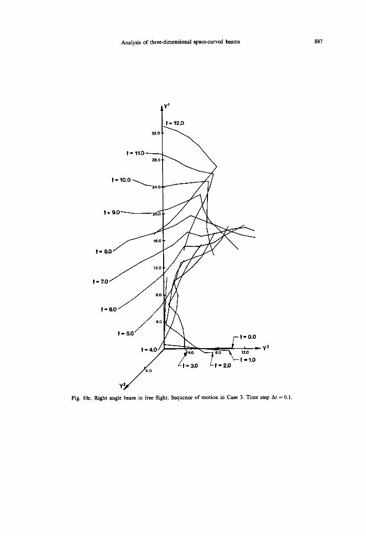
This out-of-plane problem is solved for the first time in this paper. The material properties and the load conditions used are shown in Fig. 9. The forces F, and F2 are applied at the beam axis, while the force F3 is applied at a point away from the beam axis. As

t-0.5 t 12.5

- Present

----Vu - Quoc

Fig. 4. Flexible beam in free fight, subject to constant force and constant moment. Comparison of the present results

and those of Vu-Ouoc. Time stea Ar = 0.1.


Material Properties:

EA = GA,, = lo6

El,,- El,, - GJ - lo3

Ap-1

I,, - I,, - ‘0

lime history of loading:

Fltl

0 1.0

Fig. 5. Right angle cantilever beam. Problem data.

mentioned in Sec. 5.3, if the point of application of F3 does not lie in the cross-section of the beam, it may be imagined to lie on a rigid fictitious wall fixed at the beam axis.

We analyze the three examples in which the bending and the torsional rigidities are altered so that the behavior of the beam changes from a rigid to a highly flexible body. The overall deformations obtained using 10 elements are shown in Figs lOa-10c. At time t = 0.0, the transverse force and the torsional moment are applied at point A, as shown in Fig. 9. As the beam deforms, the bending moments, in addition to the loads described above, are applied at point A. To show the bending deformations due to

these moments, the projections on the Y’-Y3 plane, of deformations of beams, with lower rigidities, are shown in Fig. 11. Even after removal of the conservative forces, remarkable bending deformations due to the F,, especially for the lowest rigidity, are observed.

As seen in this example, the total angle w at each node exceeds IL rad. Although we do not employ the four quaternion, the large deformations with finite rotations can be simulated using the conformal rotation vector or the three rotation parameters.

Table 1 shows the Euclidean norm of residual forces in the case of the beam with the lowest rigidities at time t = 2.0. In the numerical results

I”.”

1

-- 4 Elements

--- vu - Quoc

Time

Fig. 6. Right angle cantilever beam. Comparison of the present results and those of Vu-Quot. Time step Ar = 0.25.


Fig. 7. Flexible beam in free flight, subject to conservative force. Problem data.

presented in this paper the convergence rate is quadratic. This is consistent with the basic characteristic of the Newton-Raphson method.

6. CONCLUSIONS

In nonlinear dynamic analysis of beams, a number of important problems remain to be resolved. In this paper, attention has been paid to develop the nonlinear elastodynamic theory of beams and to derive the consistent linearized forms of the discrete equations. With an emphasis on the definition of the external moments, we have shown the configuration dependency of external moments. In most of the structures encountered, the external forces do not act on the beam axis itself, but on the surface of the beam. This is the case in which *the present beam theory is particularly applicable.

-I Y’

Fl 10.0

1 6.0

1 6.0

1 4.0

’ 2.0

- Example in sect. 5.3

----- Example in sect. 5.1

Fig. 8. Flexible beam in free fight, subject to conservative force. Comparison of the present problem and that in

Sec. 5.1. Time step At =O.l.

The rotation parameters ai introduced herein lead to a symmetric tangent stiffness matrix and also to a symmetric load-stiffness matrix. The AMB conditions associated with ui are different, but have forms equivalent to those derived from the static method. In the finite element formulation, the rotation parameters ai have been defined as Lagrangian components of the conformal rotation vector. As a result, as shown in the numerical results, only three

Material Properties- L

EA - GA. - lo5

AP-1 9 J,,-Jz2- 10

Case 1: El,, - El,,- GJ - 1000

Case 2: El,,- El,,- GJ = 200

Case 3: El,, - El,,- GJ - 100

F.E. Mesh: IO elements

Time history of loadingi

t F. y*/f~;~o,,o.o, F 5;$kE F: = F; - F,/5

Fig. 9. Right angle beam in free flight. Problem data.

Table 1. Euclidean norm of residual forces

Iteration number 0 1 2 3 Euclidean norm of residual 0.21505 x lo4 0.46917 x 10’ 0.20434 x 10’ 0.33963 x 1O-3

36.0

36.0

t-6.

0 4-

c

Y3

/ Y

2 Fi

g.

IOa.

Rig

ht a

ngle

bea

m i

n fr

ee R

ight

. Se

quen

ce

of m

otio

n in

Cas

e I.

T

ime

step

At

= 0

.1.

Fig.

lo

b.

Rig

ht

angl

e be

am i

n fr

ee f

light

. Se

quen

ce

of m

otio

n in

Cas

e 2.

T

ime

step

A

r =

0.1

.

,Y3

. .

7-a

_I.

c.Y

_

_ __

r,

-- ,


t

Y’

t - 12.0

t - 11.0 -

t - 7.0

t = 6.0 /

Fig. 1Oc. Right angle beam in free flight. Sequence of motion in Case 3. Time step At = 0.1


Fig. 11.

- El=100 t = 6.0

---- El= 200

L- t-o.0 Right angle beam in free flight. The projections on the Y’-Y’ plane, of deformations

with lower rigidities. of beam,

parameters are enough to describe the finite rotations 3. with a simple manipulation. The numerical results presented herein show the validity and the applica- 4. bility of the present beam theory.

Acknowledgements-The work described herein has been 5.

supported by AFOSR under contract F49620-87-C-0064. The encouragement of Dr. A. K. Amos is sincerely appre- ciated. Ms. Cindi Anderson is thanked for her assistance in

6,

the preparation of this paper.

REFERENCES 7.

1. M. Iura and S. N. Atluri, On a consistent theory, and variational formulation, of finitely stretched and rotated 8. 3-D space-curved beams. Comput. Mech. (in press).

2. S. S. Antman and K. B. Jordan, Qualitative aspects of the spatial deformation on non-linearly elastic rods. Proc. R. Sot. Edinb. 73A(5), 85-105 (1975). 9.

E. Reissner, On finite deformations of space-curved beams. J. appl. Math. Phy. (ZAMP) 32,734744 (1981). J. C. Simo and L. Vu-Quoc, A three-dimensional finite-strain rod model--II. Compuational aspects. Comput. Meth. Appl. Mech. Engng 58, 79-l 16 (1986). K. Schweizerhof and E. Ramm. Disolacement dependent pressure loads in nonlinear *finite element analysis. Comput. Struct. 18, 1099-l 114 (1984). J. H. Argyris, P. C. Dunne and D. W. Scharpf, On large displacement-small strain analysis of stuctures with rotational degrees of freedom. Comput. Meth. Appl. Mech. Engng 14, 401-451 (1978). K. J. Bathe, E. Ramm and E. L. Wilson, Finite element formulations for large deformation dynamic analysis. Int. J. Numer. Meth. Engng 9, 353-386 (1975). M. S. Gadala, G. A’E. Oravas and M. A. Dokainish, A consistent Eulerian formulation of large deformation problems in statics and dynamics. Int. J. Non-linear Mech. 18, 21-35 (1983). H. M. Koh and R. B. Haber, Elastodynamic formu-


lation of the Eulerian-Lagrangian description. J. appl. Mech. 53, 839-845 (1986).

10. L. Vu-Quoc, Dynamics of flexible structures performing large overall motions: a geometrically-nonlinear ap- proach. Electronics Research Laboratory Memor- andum UCB/ERL M86/36, University of California, Berkeley (1986).

11. M. Geradin and A. Cardona, Kinematics and dynamics of ridid and flexible mechanisms using finite elements and quaternion algebra. Comput. Me& (in press).

12. A. Rosen, R. G. Loewy and M. B. Mathew, Nonlinear dynamics of slender rods. AIAA J. 25,611419 (1987).

13. T. Belytschko and T. J. R. Hughes, Computational Methodr for Transient Analysis. Elsevier, Amsterdam (1983).

14. S. N. Atluri, Alternate stress and conjugate strain measures, and mixed variational formulations involving rigid rotations, for computational analyses of finitely

deformed solids, with application to plates and shells- 1. Theory. Comput. Struct. 18, 93-116 (1984).

15. G. R. Cowper, The shear coefficient in Timoshenko’s beam theory. J. appl. Mech. 33, 335-340 (1966).

16. K. Washizu. Varational Methods in Elasticitv and Plas- ticity, 3rd edn. Pergamon press, New York (1982).

17. J. Stuelpnagel, Dn the par~et~~tion of the three- dimensional rotation group. SIAM Rev. 6, 422-430 (1964).

18. T. R. Kane, P. W. Likins and D. A. Levinson, Space- crafi Dvnamics. McGraw-Hill. New York (1983).

19. K.” W.* Spring, Euler parameters and the use of quatemion algebra in the manipulation of finite rotations-A review. Mechanism Machine Theory 21, 365-373 (1986).

20. 0. C. Zienkiewia, The Finite Eiement Method, 3rd edn. McGraw-Hill, New York (1977).

C.A.S. 29+-K

Documents

DYNAMIC ANALYSIS OF FINITELY STRETCHED … ANALYSIS OF FINITELY STRETCHED AND ROTATED THREE-DIMENSIONAL ... dynamic analysis of finitely stretched and ... which remains a smooth space-curve