FINITELY GENERATED FREE HEYTING ALGEBRAS VIA BIRKHOFF ... · FINITELY GENERATED FREE HEYTING ALGEBRAS VIA BIRKHOFF ... algebra is built on a distributive lattice step-by ... FINITELY

Logical Methods in Computer ScienceVol. 7 (2:9) 2011, pp. 1–24www.lmcs-online.org

Submitted Oct. 5, 2010Published May 17, 2011

FINITELY GENERATED FREE HEYTING ALGEBRAS VIA BIRKHOFF

DUALITY AND COALGEBRA

NICK BEZHANISHVILI a AND MAI GEHRKE b

a Department of Computing, Imperial College Londone-mail address: [email protected]

b IMAPP, Radboud Universiteit Nijmegen, the Netherlandse-mail address: [email protected]

Abstract. Algebras axiomatized entirely by rank 1 axioms are algebras for a functorand thus the free algebras can be obtained by a direct limit process. Dually, the finalcoalgebras can be obtained by an inverse limit process. In order to explore the limits ofthis method we look at Heyting algebras which have mixed rank 0-1 axiomatizations. Wewill see that Heyting algebras are special in that they are almost rank 1 axiomatized andcan be handled by a slight variant of the rank 1 coalgebraic methods.

1. Introduction

Coalgebraic methods and techniques are becoming increasingly important in investigatingnon-classical logics, e.g., [31]. In particular, logics axiomatized by rank 1 axioms admitcoalgebraic representation as coalgebras for a functor [2], [20], [28]. We recall that an equa-tion is of rank 1 for an operation f if each variable occurring in the equation is under thescope of exactly one occurrence of f . As a result, the algebras for these logics becomealgebras for a functor over the category of underlying algebras without the operation f .Consequently, free algebras are initial algebras in the category of algebras for this functor.This correspondence immediately gives a constructive description of free algebras for rank1 logics relative to algebras in the reduced type [14], [1], [8]. Examples of rank 1 logics(relative to Boolean algebras or bounded distributive lattices) are the basic modal logicK, basic positive modal logic, graded modal logic, probabilistic modal logic, coalition logicand so on; see, e.g., [28]. For a coalgebraic approach to the complexity of rank 1 logicswe refer to [28]. On the other hand, rank 1 axioms are too simple—very few well-knownlogics are axiomatized by rank 1 axioms. Therefore, one would want to extend the existingcoalgebraic techniques to non-rank 1 logics. However, as follows from [20], algebras forthese logics cannot be represented as algebras for a functor and we cannot use the standard

1998 ACM Subject Classification: F.4.1.Key words and phrases: Heyting algebras, intuitionistic logic, free algebras, duality, coalgebra.

a Partially supported by EPSRC EP/F032102/1 and GNSF/ST08/3-397.b Partially supported by EPSRC EP/E029329/1 and EP/F016662/1.

LOGICAL METHODSl IN COMPUTER SCIENCE DOI:10.2168/LMCS-7 (2:9) 2011c© N. Bezhanishvili and M. GehrkeCC© Creative Commons

http://creativecommons.org/about/licenses

2 N. BEZHANISHVILI AND M. GEHRKE

construction of free algebras in a straightforward way.

This paper is an extended version of [7]. However, unlike [7], here we give a complete so-lution to the problem of describing finitely generated free Heyting algebras in a systematicway using methods similar to those used for rank 1 logics. This paper together with [7]and [8] is a facet of a larger joint project with Alexander Kurz on coalgebraic treatmentof modal logics beyond rank 1. We recall that an equation is of rank 0-1 for an operationf if each variable occurring in the equation is under the scope of at most one occurrenceof f . With the ultimate goal of generalizing a method of constructing free algebras forvarieties axiomatized by rank 1 axioms to the case of rank 0-1 axioms, we consider the caseof Heyting algebras (intuitionistic logic, which is of rank 0-1 for f =→). In particular, weconstruct free Heyting algebras. For an extension of coalgebraic techniques to deal with thefinite model property of non-rank 1 logics we refer to [25].

Free Heyting algebras have been the subject of intensive investigation for decades. Theone-generated free Heyting algebra was constructed in [26] and independently in [22]. Analgebraic characterization of finitely generated free Heyting algebras is given in [30]. A verydetailed description of finitely generated free Heyting algebras in terms of their dual spaceswas obtained independently in [29], [17], [4] and [27]. This method is based on a descriptionof the points of finite depth of the dual frame of the free Heyting algebra. For a detailedoverview of this construction we refer to [12, Section 8.7] and [6, Section 3.2]. Finally, [13]introduces a different method for describing free Heyting algebras. In [13] the free Heytingalgebra is built on a distributive lattice step-by-step by freely adding to the original latticethe implications of degree n, for each n ∈ ω. [13] uses this technique to show that everyfinitely generated free Heyting algebra is a bi-Heyting algebra. A more detailed accountof this construction, which we call Ghilardi’s construction or Ghilardi’s representation, canbe found in [10] and [16]. Based on this method, [16] derives a model-theoretic proof ofPitts’ uniform interpolation theorem. In [3] a similar construction is used to describe freelinear Heyting algebras over a finite distributive lattice and [24] applies the same methodto construct higher order cylindric Heyting algebras. Recently, in [15] this approach wasextended to S4-algebras of modal logic. We also point out that in [14] a systematic studyis undertaken on the connection between constructive descriptions of free modal algebrasand the theory of normal forms.

Our contribution is to derive Ghilardi’s representation of finitely generated free Heytingalgebras in a modular way which is based entirely on the ideas of the coalgebraic approachto rank 1 logics, though it uses these ideas in a non-standard way. We split the processinto two parts. We first apply the initial algebra construction to weak and pre-Heytingalgebras—these are consecutive rank 1 approximants of Heyting algebras. We then use anon-standard colimit system based on the sequence of algebras for building free pre-Heytingalgebras in the standard coalgebraic framework.

The closest approximants of the rank 1 reducts of Heyting algebras appearing in the lit-erature are weak Heyting algebras introduced in [11]. This is in fact why we first treatweak Heyting algebras. However, Heyting algebras satisfy more rank 1 axioms, namely atleast those of what we call pre-Heyting algebras. While we identified these independentlyin this work, these were also identified by Dito Pataraia, also in connection with the study

FINITELY GENERATED FREE HEYTING ALGEBRAS VIA BIRKHOFF DUALITY AND COALGEBRA 3

of Ghilardi’s construction1. The fact that the functor for which pre-Heyting algebras arealgebras yields Ghilardi’s representation by successive application and quotienting out well-definition of implication is, to the best of our knowledge, new to this paper.

On the negative side, we use some properties particular to Heyting algebras, and thus ourwork does not yield a method that applies in general. Nevertheless, we expect that theapproach, though it would have to be tailored, is likely to be successful in other instancesas well. Obtained results allow us to derive a coalgebraic representation for weak and pre-Heyting algebras and sheds new light on the very special nature of Heyting algebras.

The paper is organized as follows. In Section 2 we recall the so-called Birkhoff (discrete)duality for distributive lattices. We use this duality in Section 3 to build free weak Heytingalgebras and in Section 4 to build free pre-Heyting algebras. Obtained results are appliedin Section 5 for describing free Heyting algebras. In Section 6 we give a coalgebraic repre-sentation for weak and pre-Heyting algebras. We conclude the paper by listing some futurework.

2. Discrete duality for distributive lattices

We recall that a bounded distributive lattice is a distributive lattice with the least andgreatest elements 0 and 1, respectively. Throughout this paper we assume that all thedistributive lattices are bounded. We also recall that a non-zero element a of a distributivelattice D is called join-irreducible if for every b, c ∈ D we have that a ≤ b ∨ c implies a ≤ bor a ≤ c. For each distributive lattice (DL for short) D let (J(D),≤) denote the subposetof D consisting of all join-irreducible elements of D. Recall also that for every poset X asubset U ⊆ X is called a downset if x ∈ U and y ≤ x imply y ∈ U . For each poset Xwe denote by O(X) the distributive lattice (O(X),∩,∪, ∅,X) of all downsets of X. FiniteBirkhoff duality tells us that every finite distributive lattice D is isomorphic to the latticeof all downsets of (J(D),≤) and vice versa, every finite poset X is isomorphic to the posetof join-irreducible elements of O(X). We call (J(D),≤) the dual poset of D and we callO(X) the dual lattice of X.

Recall that a lattice morphism is called bounded if it preserves 0 and 1. Unless statedotherwise all the lattice morphisms will be assumed to be bounded. The duality betweenfinite distributive lattices and finite posets can be extended to the duality between thecategory DLfin of finite distributive lattices and lattice morphisms and the category Posfinof finite posets and order-preserving maps. In fact, if h : D → D′ is a lattice morphism,then the restriction of h♭, the lower adjoint of h, to J(D′) is an order-preserving mapbetween (J(D′),≤′) and (J(D),≤), and if f : X → X ′ is an order-preserving map betweentwo posets X and X ′, then f↓ : O(X) → O(X ′), S 7→ ↓f(S) is

∨-preserving and its

upper adjoint (f↓)♯ = f−1 : O(X ′) → O(X) is a lattice morphism. Moreover, injectivelattice morphisms (i.e. embeddings or, equivalently, regular monomorphisms) correspond tosurjective order-preserving maps, and surjective lattice morphisms (homomorphic images)correspond to order embeddings (order-preserving and order-reflecting injective maps) thatare in one-to-one correspondence with subposets of the corresponding poset. A particularcase of this correspondence that will be used repeatedly throughout this paper is spelledout in the following proposition.

1Private communication with the first listed author.


Proposition 2.1. Let D be a finite distributive lattice, X = (J(D),≤) its dual poset, and

a, b ∈ D. The least-collapsed quotient of D in which a ≤ b is the dual lattice of the subposet

of X based on the set {y ∈ X | y ≤ a =⇒ y ≤ b}.

Proof. By Birkhoff duality, every quotient of D corresponds to a subposet of X. For anysubposet Y ⊆ X, the dual quotient is given by

O(X) → O(Y )

U 7→ U ∩ Y.

For a, b ∈ D, a corresponds to the downset a = {x ∈ X | x ≤ a} and similarly for b and wehave

a ∩ Y ⊆ b ∩ Y ⇐⇒ ∀y ∈ Y (y ≤ a =⇒ y ≤ b).

Clearly, the largest subset Y for which this is true is Y = {y ∈ X | y ≤ a =⇒ y ≤ b}.

We will also need the following fact.

Proposition 2.2. Let X be a finite set and FDL(X) the free distributive lattice over X.

Then the poset (J(FDL(X)),≤) of join-irreducible elements of FDL(X) is isomorphic to

(P(X),⊇), where P(X) is the powerset of X and each subset S ⊆ X corresponds to the

conjunction∧S ∈ FDL(X). Moreover, for x ∈ X and S ⊆ X we have∧

S ≤ x iff x ∈ S.

Proof. This is equivalent to the disjunctive normal form representation for elements ofFDL(X).

Finally we recall that an element a 6= 1 in a distributive lattice D is called meet-

irreducible provided, for every b, c ∈ D, we have that b ∧ c ≤ a implies b ≤ a or c ≤ a. Welet M(D) denote the set of all meet-irreducible elements of D.

Proposition 2.3. Let D be a finite distributive lattice. Then for each p ∈ J(D), there

exists κ(p) ∈M(D) such that p � κ(p) and for each a ∈ D we have

p ≤ a or a ≤ κ(p).

Proof. For p ∈ J(D), let κ(p) =∨{a ∈ D | p � a}. Then it is clear that the condition

involving all a ∈ D holds. Note that if p ≤ κ(p) =∨{a ∈ D | p � a}, then, applying the

join-irreducibility of p, we get a ∈ D with p � a but p ≤ a, which is clearly a contradiction.So it is true that p � κ(p). Now we show that κ(p) is meet irreducible. First note thatsince p is not below κ(p), the latter cannot be equal to 1. Also, if a, b � κ(p) then p ≤ a, band therefore p ≤ a ∧ b. Thus it follows that a ∧ b � κ(p). This concludes the proof of theproposition.

Remark 2.4. Note that p and κ(p) satisfying the condition of Proposition 2.3 are calleda splitting and co-splitting elements of D, respectively. The notions of splitting and co-splitting elements were introduced in lattice theory by Whitman [32]. It is easy to seethat if for p ∈ D there exists κ′(p) ∈ D satisfying the condition of Proposition 2.3, thenκ′(p) = κ(p). Therefore, κ(p) ∈ D, satisfying the condition of Proposition 2.3, is unique.


3. Weak Heyting algebras

In this section we introduce weak Heyting algebras and describe finitely generated free weakHeyting algebras.

3.1. Freely adding weak implications.

Definition 3.1. [11] A pair (A,→) is called a weak Heyting algebra2, wHA for short, if Ais a distributive lattice and →: A2 → A is a weak implication, that is, a binary operationsatisfying the following axioms for all a, b, c ∈ A:

(1) a→ a = 1,(2) a→ (b ∧ c) = (a→ b) ∧ (a→ c).(3) (a ∨ b)→ c = (a→ c) ∧ (b→ c).(4) (a→ b) ∧ (b→ c) ≤ a→ c.

It is easy to see that by (2) weak implication is order-preserving in the second coordinateand by (3) order-reversing in the first. The following lemma gives a few useful propertiesof wHAs.

Lemma 3.2. Let (A,→) be a wHA. For each a, b ∈ A we have

(i) a→ b = a→ (a ∧ b),

(ii) 1→ (a→ b) ≤ (1→ a)→ (1→ b).

Proof. (i) By axiom (2) we have a→ (a∧ b) = (a→ a)∧ (a→ b) and by axiom (1) we havea→ a = 1 so we obtain a→ b = a→ (a ∧ b).

(ii) Since the weak implication→ is order-reversing in the first coordinate and 1 ≥ 1→ awe have 1 → (a → b) ≤ (1 → a) → (a → b). By (i) of this lemma we obtain (1 → a) →(a→ b) = (1→ a)→ [(1→ a)∧ (a→ b)]. Now axiom (4) yields (1→ a)∧ (a→ b) ≤ 1→ b.So (1 → a) → (a → b) ≤ (1 → a) → (1 → b). By transitivity of the order we have thedesired result.

Let D and D′ be distributive lattices. We let _(D × D) denote the set {a _ b : a ∈ Dand b ∈ D′}. We stress that this is just a set bijective with D ×D′. The symbol _ is justa formal notation. For each distributive lattice D we let FDL(_(D ×D)) denote the freedistributive lattice over _(D ×D). Moreover, we let

H(D) = FDL(_(D ×D))/≈

where ≈ is the DL congruence generated by the axioms (1)–(4) seen as relation schemasfor _. The point of view is that of describing a distributive lattice by generators andrelations. That is, we want to find the quotient of the free distributive lattice over the set_ (D × D) with respect to the lattice congruence generated by the pairs of elements ofFDL(_ (D×D)) in (1)–(4) (where → is replaced by _) with a, b, c ranging over D. For anelement a _ b ∈ FDL(_ (D×D)) we denote by [a _ b]≈ the ≈ equivalence class of a _ b.

The rest of this subsection will be devoted to showing that for each finite distributivelattice D the poset (J(H(D)),≤) is isomorphic to (P(J(D)),⊆). Below we give a dualproof of this fact. The dual proof, which relies on the fact that identifying two elementsof an algebra simply corresponds to throwing out those points of the dual that are belowone and not the other (Proposition 2.1), is produced in a modular and systematic way that

2In [11] weak Heyting algebras are called ‘weakly Heyting algebras’.


does not require any prior insight into the structure of these particular algebras.

We start with a finite distributive lattice D and the free DL generated by the set

_ (D ×D) = {a _ b | a, b ∈ D}

of all formal arrows over D. As follows from Proposition 2.2, J(FDL(_ (D × D))) isisomorphic to the powerset of _ (D × D), ordered by reverse inclusion. Each subsetS ⊆_ (D ×D) corresponds to the conjunction

∧S of the elements of S; the empty set of

course corresponds to 1. Now we want to take quotients of this free distributive lattice withrespect to various lattice congruences, namely the ones generated by the set of instances ofthe axioms for weak Heyting algebras.

The relational schema x _ x ≈ 1.

Here we want to take the quotient of FDL(→ (D×D)) with respect to the lattice congruenceof FDL(→ (D × D)) generated by the set {(a _ a, 1) | a ∈ D}. By Proposition 2.1 thisquotient is given dually by the subposet, call it P1, of our initial poset P0 = J(FDL(→ (D×D))), consisting of those join-irreducibles of FDL(→ (D×D)) that do not violate this axiom.Thus, for S ∈ J(FDL(→ (D ×D))), S is admissible provided

∀a ∈ D (∧

S ≤ 1 ⇐⇒∧

S ≤ a _ a).

Since all join-irreducibles are less than or equal to 1, it follows that the only join-irreduciblesthat are admissible are the ones that are below a _ a for all a ∈ D. That is,viewed assubsets of _ (D ×D), only the ones that contain a _ a for each a ∈ D:

P1 = {S ∈ P0 | a _ a ∈ S for each a ∈ D}.

The relational schema x _ (y ∧ z) ≈ (x _ y) ∧ (x _ z).

We now want to take a further quotient and thus we want to keep only those join-irreduciblesfrom P1 that do not violate this relational schema. That is, S ∈ P1 is admissible provided

∀a, b, c (∧

S ≤ a _ (b ∧ c) ⇐⇒∧

S ≤ a _ b and∧

S ≤ a _ c).

which means

∀a, b, c (a _ (b ∧ c) ∈ S ⇐⇒ a _ b ∈ S and a _ c ∈ S).

Let P2 denote the poset of admissible join-irreducible elements of P1.

Proposition 3.3. The poset P2 is order isomorphic to the set

Q2 = {f : D → D | ∀a ∈ D, f(a) ≤ a}

ordered pointwise.

Proof. An admissible S from P2 corresponds to the function fS : D → D given by

fS(a) =∧{b ∈ D | a _ b ∈ S}.

In the reverse direction, a function in Q2 corresponds to the admissible set

Sf = {a _ b | f(a) ≤ b}.

The proof that this establishes an order isomorphism is a straightforward verification.


The relational schema (x ∨ y) _ z ≈ (x _ z) ∧ (y _ z).

We want the subposet of Q2 consisting of those f ’s such that

∀a, b, c((a ∨ b) _ c ∈ Sf ⇐⇒ a _ c ∈ Sf and b _ c ∈ Sf

).

To this end notice that

∀a, b, c((a ∨ b) _ c ∈ Sf ⇐⇒ (a _ c ∈ Sf and b _ c ∈ Sf )

)

⇐⇒ ∀a, b, c(f(a ∨ b) ≤ c ⇐⇒ (f(a) ≤ c and f(b) ≤ c)

)

⇐⇒ ∀a, b f(a ∨ b) = f(a) ∨ f(b).

That is, the poset P3 of admissible join-irreducibles left at this stage is isomorphic to theset

Q3 = {f : D → D | f is join-preserving and ∀a ∈ D f(a) ≤ a}.

The relational schema (x _ y) ∧ (y _ z) w x _ z.

It is not hard to see that this yields, in terms of join-preserving functions f : D → D,

Q4 = {f ∈ Q3 | ∀a ∈ D f(a) ≤ f(f(a))}

= {f : D → D | f is join-preserving and ∀a ∈ D f(a) ≤ f(f(a)) ≤ f(a) ≤ a}

= {f : D → D | f is join-preserving and ∀a ∈ D f(f(a)) = f(a) ≤ a}.

We note that the elements of Q4 are nuclei [18] on the order-dual lattice of D. Since thef ’s in Q4 are join and 0 preserving, they are completely given by their action on J(D). Theadditional property shows that these functions have lots of fixpoints. In fact, we can showthat they are completely described by their join-irreducible fixpoints.

Lemma 3.4. Let f ∈ Q4, then for each a ∈ D we have

f(a) =∨{r ∈ J(D) | f(r) = r ≤ a}.

Proof. Clearly∨{r ∈ J(D) | f(r) = r ≤ a} ≤ f(a). For the converse, let r be maximal in

J(D) with respect to the property that r ≤ f(a). Now it follows that

r ≤ f(a) = f(f(a)) =∨{f(q) | J(D) ∋ q ≤ f(a)}.

Since r is join-irreducible, there is q ∈ J(D) with q ≤ f(a) and r ≤ f(q). Thus r ≤ f(q) ≤q ≤ f(a) and by maximality of r we conclude that q = r. Now r ≤ f(q) and q = r yieldsr ≤ f(r). However, f(r) ≤ r as this holds for any element of D and thus f(r) = r. Sinceany element in a finite lattice is the join of the maximal join-irreducibles below it, we obtain

f(a) =∨{r ∈ J(D) | r is maximal in J(D) with respect to r ≤ f(a)}

≤∨{r ∈ J(D) | f(r) = r ≤ f(a)} ≤ f(a).

Finally, notice that if f(r) = r ≤ f(a) then as f(a) ≤ a, we have f(r) = r ≤ a. Conversely,if f(r) = r ≤ a then r = f(r) = f(f(r)) ≤ f(a) and we have proved the lemma.


Proposition 3.5. The set of functions in Q4, ordered pointwise, is order isomorphic to the

powerset of J(D) in the usual inclusion order.

Proof. The order isomorphism is given by the following one-to-one correspondence

Q4 ⇆ P(J(D))

f 7→ {p ∈ J(D) | f(p) = p}

fT ← [ T

where fT : D → D is given by fT (a) =∨{p ∈ J(D) | T ∋ p ≤ a}. Using Lemma 3.4, it is

straightforward to see that these two assignments are inverse to each other. Checking thatfT is join preserving and satisfies f2 = f ≤ idD is also straightforward. Finally, it is clearthat fT ≤ fS if and only if T ⊆ S.

Next we will prove a useful lemma that will be applied often throughout the remainder ofthis paper. Let D be a finite distributive lattice. For a, b ∈ D and T ⊆ J(D) we writeT � a _ b provided

∧ST ≤ a _ b, where ST = SfT = {a _ b : fT (a) ≤ b}.

Lemma 3.6. Let D be a finite distributive lattice. For each a, b ∈ D and T ⊆ J(D) we

have

T � a _ b iff ∀p ∈ T (p ≤ a implies p ≤ b)

Proof.

T � a _ b ⇐⇒∧

ST ≤ a _ b

⇐⇒ a _ b ∈ ST

⇐⇒ fT (a) ≤ b

⇐⇒∨

(↓a ∩ T ) ≤ b

⇐⇒ ∀p ∈ T (p ≤ a implies p ≤ b).

This subsection culminates in the following theorem. Recall that, for a join-irredu-cible q of a finite distributive lattice, κ(q) is the corresponding meet irreducible, recallProposition 2.3.

Theorem 3.7. Let D be a finite distributive lattice and X = (J(D),≤) its dual poset. Then

the following statements are true:

(i) The poset (J(H(D)),≤) is isomorphic to the poset (P(X),⊆) of all subsets of Xordered by inclusion.

(ii) J(H(D)) = {[∧

q 6∈T (q _ κ(q))]≈ | T ⊆ X}.

Proof. As shown above, the poset J(H(D)), obtained from J(FDL(_(D×D))) by removingthe elements that violate the relational schemas obtained from axioms (1)–(4), is isomor-phic to the poset Q4, and Q4 is in turn isomorphic to P(J(D)) ordered by inclusion, seeProposition 3.5.

In order to prove the second statement, let q ∈ J(D), and consider q _ κ(q) ∈ FDL(_(D×D)). If we represent H(D) as the lattice of downsets O(J(H(D))), then the action of


the quotient map on this element is given by

FDL(_ (D ×D)) → H(D)

q _ κ(q) 7→ {T ′ ∈ P(J(D)) | q _ κ(q) ∈ ST ′}.

Nowq _ κ(q) ∈ ST ′ ⇐⇒ fT ′(q) ≤ κ(q)

⇐⇒∨

(↓q ∩ T ′) ≤ κ(q)

⇐⇒ q 6∈ T ′.

The last equivalence follows from the fact that a ≤ κ(q) if and only if q � a and the onlyelement of ↓q that violates this is q itself (Proposition 2.3). We now can see that for anyT ⊆ J(D) we have

FDL(→ (D ×D)) → H(D)

[∧

q 6∈T

(q _ κ(q))]≈ 7→ {T ′ ∈ P(J(D)) | ∀q (q 6∈ T ⇒ q _ κ(q) ∈ ST ′)}

= {T ′ ∈ P(J(D)) | ∀q (q 6∈ T ⇒ q 6∈ T ′)}

= {T ′ ∈ P(J(D)) | ∀q (q ∈ T ′ ⇒ q ∈ T )}

= {T ′ ∈ P(J(D)) | T ′ ⊆ T}.

That is, under the quotient map FDL(→ (D×D)) → H(D), the elements∧

q 6∈T (q _ κ(q))

are mapped to the principal downsets ↓T , for each T ∈ P(J(D)) = J(H(D)). Since theseprincipal downsets are exactly the join-irreducibles of O(J(H(D))) = H(D), we have that{ [

∧q 6∈T (q _ κ(q))]≈ | T ⊆ J(D) } = J(H(D)).

It follows from Theorem 3.7(1) that if two finite distributive lattices D and D′ have anequal number of join-irreducible elements, then H(D) is isomorphic to H(D′). To see this,we note that if |J(D)| = |J(D′)|, then (P(J(D)),⊆) is isomorphic to (P(J(D′)),⊆). This,by Theorem 3.7(1), implies that H(D) is isomorphic to H(D′). In particular, any two non-equivalent orders on any finite set give rise to two non-isomorphic distributive lattices withisomorphic H-images.

Remark 3.8. All the results in this section for finite distributive lattices can be generalizedto the infinite case. In the infinite case, however, instead of finite posets we would needto work with Priestley spaces and instead of the finite powerset we need to work with theVietoris space (see Section 6). As we will see in Sections 3.2, 4 and 5, for our purposes (thatis, for describing finitely generated free weak Heyting, pre-Heyting and Heyting algebras),it suffices to work with limits of finite distributive lattices. So we will stick with the finitecase, for now, and will consider infinite distributive lattices and Priestley spaces only inSection 6, where we discuss coalgebraic representation of weak Heyting and pre-Heytingalgebras.


3.2. Free weak Heyting algebras. In the coalgebraic approach to generating the freealgebra, it is a fact of central importance that H as described here is actually a functor.That is, for a DL homomorphism h : D → E one can define a DL homomorphism H(h) :H(D) → H(E) so that H becomes a functor on the category of DLs. To see this, we onlyneed to note that H is defined by rank 1 axioms. We recall that for an operator f (in ourcase f is the weak implication →) an equation is of rank 1 if each variable in the equationis under the scope of exactly one occurrence of f and an equation is of rank 0-1 if eachvariable in the equation is under the scope of at most one occurrence of f . It is easy tocheck that axioms (1)–(4) for weak Heyting algebras are rank 1. Therefore, H gives rise toa functor H : DL → DL, where DL is the category of all distributive lattices and latticemorphisms. (This fact can be found in [2], for Set-functors, and in [20] for the general case.)Moreover, the category of weak Heyting algebras is isomorphic to the category Alg(H) ofthe algebras for the functor H. For the details of such correspondences we refer to either of[1], [2], [8], [14], [20]. We would like to give a concrete description of how H applies to DLhomomorphisms. We describe this in algebraic terms here and give the dual constructionvia Birkhoff duality.

Let h : D → E be a DL homomorphism. Recall that the dual map from J(E) to J(D)

is just the lower adjoint h♭ with domain and codomain properly restricted. By abuse ofnotation we will just denote this map by h♭, leaving it to the reader to decide what theproper domain and codomain is. Now H(D) = FDL(_ (D × D))/ ≈D, where ≈D is theDL congruence generated by the set of all instances of the axioms (1)–(4) with a, b, c ∈ D.Also let qD be the quotient map corresponding to quotienting out by ≈D. Any latticehomomorphism

h : D → E

yields a maph× h : D ×D −→ E × E

and this of course yields a lattice homomorphism

FDL(h× h) : FDL(_ (D ×D)) −→ FDL(_ (E ×E)).

Now the point is that FDL(h × h) carries elements of ≈D to elements of ≈E (it is an easyverification and only requires h to be a homomorphism for axiom schemas (2) and (3)).Thus we have ≈D⊆ Ker(qE ◦ FDL(h × h)) or equivalently that there is a unique mapH(h) : H(D)→ H(E) that makes the following diagram commute

FDL(→ (D ×D))FDL(h×h) //

qD��

FDL(→ (E × E))

qE��

H(D)H(h)

//____________ H(E).

The dual diagram is

P(D ×D) oo(h×h)−1

P(E × E)

P(J(D))� ?

eD

OO

oo P(h♭)_______ P(J(E))

� ?

eE

OO

The map eD : P(D) → P(D ×D) is the embedding, via Q4 and so on into P0 as obtainedabove. That is, eD(T ) = {a → b | ∀p ∈ T (p ≤ a ⇒ p ≤ b)}. Now in this dual setting, the

FINITELY GENERATED FREE HEYTING ALGEBRAS VIA BIRKHOFF DUALITY AND COALGEBRA11

fact that there is a map P(h♭) is equivalent to the fact that (h × h)−1 ◦ eE maps into theimage of the embedding eD. This is easily verified:

(h× h)−1(eE(T )) = {a→ b | ∀q ∈ T (q ≤ h(a)⇒ q ≤ h(b))}

= {a→ b | ∀q ∈ T (h♭(q) ≤ a⇒ h♭(q) ≤ b)}

= {a→ b | ∀p ∈ h♭(T ) (p ≤ a⇒ p ≤ b)}

= eD(h♭(T )).

Thus we can read off directly what the map P(h♭) is: it is just forward image under h♭.That is, if we call the dual of h : D → E by the name f : J(E) → J(D), then P(f) = f [ ]where f [ ] is the lifted forward image mapping subsets of J(E) to subsets of J(D). Finally,we note that P(f) is an embedding if and only if f is injective, and P(f) is surjective ifand only if f is surjective.

Remark 3.9. It follows from Theorem 3.7(i) that the functor H can be represented as acomposition of two functors. Let B : DLfin → BAfin be the functor from the category offinite distributive lattices to the category of finite Boolean algebras which maps every finitedistributive lattice to its free Boolean extension—the (unique) Boolean algebra generatedby this distributive lattice. It is well known [21] that the dual of the functor B is theforgetful functor from the category of finite posets to the category of finite sets, which mapsevery finite poset to its underlying set. Further, let also HB : BAfin → DLfin be the functorH restricted to Boolean algebras. That is, given a Boolean algebra A we define HB(A) asthe free DL over _(B,B) quotiented out by the relational schemas corresponding to theaxioms (1)–(4) of wHAs. Then the functor which is dual to HB maps each finite set X to(P(X),⊆) and therefore H : DLfin → DLfin is the composition of B with HB.

Since weak Heyting algebras are the algebras for the functor H, we can make use ofcoalgebraic methods for constructing free weak Heyting algebras. Similarly to [8], wherefree modal algebras and free distributive modal algebras were constructed, we constructfinitely generated free weak Heyting algebras as initial algebras of Alg(H). That is, wehave a sequence of distributive lattices, each embedded in the next:

n −→ FDL(n), the free distributive lattice on n generators,

D0 = FDL(n),

Dk+1 = D0 +H(Dk), where + is the coproduct in DL,

i0 : D0 → D0 +H(D0) = D1 the embedding given by coproduct,

ik : Dk → Dk+1 where ik = idD0+H(ik−1).

For a, b ∈ Dk, we denote by a→k b the equivalence class [a _ b]≈ ∈ H(Dk) ⊆ Dk+1. Now,by applying the technique of [1], [2], [8] [14], to weak Heyting algebras, we arrive at thefollowing theorem.

Theorem 3.10. The direct limit (Dω, (Dk → Dω)k) in DL of the system (Dk, ik : Dk →Dk+1)k with the binary operation →ω: Dω × Dω → Dω defined by a →ω b = a →k b,for a, b ∈ Dk is the free n-generated weak Heyting algebra when we embed n in Dω via

n→ D0 → Dω.

Now we will look at the dual of (Dω,→ω). Let X0 = P(n) be the dual of D0 and let

Xk+1 = X0 × P(Xk)


be the dual of Dk+1.

Theorem 3.11. The sequence (Xk)k<ω with maps πk : X0 × P(Xk)→ Xk defined by

πk = idX0× P(πk−1) i.e. πk(x,A) = (x, πk−1[A])

is dual to the sequence (Dk)k<ω with maps ik : Dk → Dk+1. In particular, the πk’s are

surjective.

Proof. The dual of D0 is X0 = P(n), and since Dk+1 = D0 + H(Dk), it follows thatXk+1 = X0 × P(Xk) as sums go to products and as H is dual to P. For the maps,π0 : X0 × P(X0) → X0 is just the projection onto the first coordinate since i0 is theinjection given by the sum construction. We note that π0 is surjective. Now the dualπk : Xk+1 = X0×P(Xk)→ Xk = X0×P(Xk−1) of ik = idD0

+H(ik−1) is idX0×P(πk−1),

which is exactly the map given in the statement of the theorem. Note that a map of theform X × Y → X × Z given by (x, y) 7→ (x, f(y)), where f : Y → Z is surjective if andonly the map f is. Also, as we saw above, P(πk) is surjective if and only if πk is. Thus byinduction, all the πk’s are surjective.

4. Pre-Heyting algebras

In this section we define pre-Heyting algebras which form a subvariety of weak Heytingalgebras and describe free pre-Heyting algebras. We first note that, for any weak Heytingalgebra A, the map from A to A given by a 7→ (1 → a) is meet-preserving and alsopreserves 1 by virtue of the first two axioms of weak Heyting algebras. For the same reason,the map from a distributive lattice D to H(D) mapping each element a of D to [1 _ a]≈also is meet-preserving and preserves 1. For Heyting algebras more is true: for a Heytingalgebra B, the map given by b 7→ (1→ b) is just the identity map and thus, in particular,it is a lattice homomorphism. In other words, Heyting algebras satisfy additional rank 1axioms beyond those of weak Heyting algebras.

Definition 4.1. A weak Heyting algebra (A,→) is called a pre-Heyting algebra, pHA forshort, if the following additional axioms are satisfied for all a, b ∈ A:

(5) 1→ 0 = 0,(6) (1→ a) ∨ (1→ b) = 1→ (a ∨ b).

Since these are again rank 1 axioms, we can obtain a description of the free finitelygenerated pre-Heyting algebras using the same method as for weak Heyting algebras. Ac-cordingly, for a finite distributive lattice D, similarly to what we did in the previous section,we let

K(D) = FDL(→ (D ×D))/≅where ≅ is the DL congruence generated by the axioms (1)–(6) viewed as relational schemasfor FDL(→ (D ×D)). This of course means we can just proceed from where we left off inSection 3 and identify the further quotient of H(D) obtained by the schema (1 _ a)∨ (1 _

b) ≅ 1 _ (a ∨ b) for a and b ranging over the elements of D and 1 _ 0 ≅ 0. That is, weneed to calculate

K(D) = H(D)/≃where ≃ is the DL congruence given by the relational schemas obtained from the axioms(5)–(6).


We say that a subset S of a poset (X,≤) is rooted if there exists p ∈ S, which we callthe root of S, such that q ≤ p for each q ∈ S. It follows from the definition that a root of arooted set is unique. Also a rooted set is necessarily non-empty. We denote by Pr(X) theset of all rooted subsets of (X,≤). We also let

root : Pr(X)→ X

be the map sending each rooted subset S of X to its root. It is easy to see that root issurjective and order-preserving.

Theorem 4.2. Let D be a finite distributive lattice and X its dual poset. Then the following

statements are true:

(i) The poset (J(K(D)),≤) is isomorphic to the poset (Pr(X),⊆) of all rooted subsets of

X ordered by inclusion.

(ii) J(K(D)) = {[(1 _ x) ∧ (∧

q<x,q 6∈T ′(q _ κ(q))]≅ | T′ ⊆ ↓x \ {x}, x ∈ X}.

(iii) The map D → K(D) given by a 7→ [1 _ a]≅ is an injective lattice homomorphism

whose dual is the surjective order-preserving map root : Pr(X)→ X.

Proof. (i) By Theorem 3.7(i), (J(H(D)),≤) is isomorphic to (P(X),⊆). Thus, we need toshow that the rooted subsets of X are exactly the subsets which are admissible with respectto relational schemas given by the axioms (5) and (6). For the axiom (5), it may be worthclarifying the meaning of this relational schema: the 0 (and 1) on the left side are elementsof D, and the expression 1 _ 0 is one of the generators of FDL(→ (D×D)), whereas the 0on the right of the equality is the bottom of the lattice H(D) — we will denote it by 0H(D)

for now. A set S ⊆ X is admissible for (5) provided

S � 1 _ 0 ⇐⇒ S � 0H(D).

Now by Lemma 3.6, S � 1 _ 0 if and only if, for all p ∈ S, p ≤ 1 implies p ≤ 0. Sincethe former is true for every p ∈ X and the latter is false for all p ∈ X, the only S ∈ P(X)satisfying this condition is S = ∅. On the other hand, as in any lattice, no join-irreduciblein K(D) is below 0K(D). Thus (5) eliminates S = ∅.

Weak Heyting implication is meet-preserving and thus order-preserving in the secondcoordinate so that we have that 1 _ (a∨ b) ≥ (1 _ a)∨ (1 _ b) already in H(D) for everyD. Therefore, a set S ⊆ X is admissible with respect to (5) and (6) iff S 6= ∅ and

S � 1 _ (a ∨ b) implies S � 1 _ a or S � 1 _ b.

Now by Lemma 3.6, S � 1 _ x iff S ⊆ ↓x, so for non-empty S we need S ⊆ ↓(a ∨ b)to imply that S ⊆ ↓a or S ⊆ ↓b for all a, b ∈ D. This is easily seen to be equivalent torootedness: If S ⊆ X is rooted and p is its root, then S ⊆ ↓(a ∨ b) implies p ≤ a ∨ b. Thus,p ≤ a or p ≤ b and so S ⊆ ↓a or S ⊆ ↓b. Conversely, if S is admissible then S 6= ∅ and, asit is finite, every element of S is below a maximal element of S. If p ∈ S is maximal butnot the maximum of S then S ⊆ ↓(p ∨ a), where a =

∨(S \ {p}), but S 6⊆ ↓p and S 6⊆ ↓a.

(ii) The proof is similar to the proof of Theorem 3.7(ii). Recall that for any T ⊆ X wehave that the join-irreducible {T ′ ∈ P(X) | T ′ ⊆ T} = ↓T in O(P(X)), which is isomorphicto H(D), is equal to [

∧q 6∈T (q _ κ(q))]≈. Also [1 _ x]≈ is join-irreducible and corresponds

to ↓x ⊆ X. That is,

[1 _ x]≈ = [∧

q�x

(q _ κ(q))]≈.


Thus, in particular, for T ⊆ X rooted with root x and T ′ = T \ {x}, the join-irreduciblecorresponding to T is given by

[∧

q 6∈T

(q _ κ(q)]≈ = [∧

q�x

(q _ κ(q)) ∧∧

q≤x,q 6∈T

(q _ κ(q))]≈

= [(1 _ x) ∧∧

q<x,q 6∈T ′

(q _ κ(q))]≈.

Since this is the case in H(D), it is certainly also true in the further quotient K(D) andin (i) we have shown that all join-irreducibles of K(D) correspond to rooted subsets of X,thus the statement follows.

(iii) The map D → K(D) given by a 7→ [1 _ a]≅ is clearly a homomorphism since wehave quotiented out by all the necessary relations: [1 _ 1]≅ = 1K(D) by (1), [1 _ 0]≅ =0K(D) by (5), and the map is meet and join preserving by (2) and (6), respectively. Aswe saw in Section 2, the dual of a homomorphism between finite lattices is the restrictionto join-irreducibles of its lower adjoint, that is, our homomorphism is dual to the mapr : Pr(X)→ X given by

∀T ∈ Pr(X) ∀a ∈ D (r(T ) ≤ a ⇐⇒ T � (1 _ a)).

For T ∈ Pr(X) we have T � (1 _ a) =∨

x∈X,x≤a(1 _ x) if and only if there is an x ∈ X

with x ≤ a and T � (1 _ x). Furthermore T � (1 _ x) if and only if T ⊆ ↓ x if and only ifroot (T ) ≤ x. That is, r(T ) ≤ a if and only if root(T ) ≤ a so that, indeed, root (T ) = r(T ).It is clear that the map root is surjective and thus the dual homomorphism D → K(D) isinjective.

The following proposition will be used to obtain some important results in the next sectionof this paper.

Proposition 4.3. Let D be a finite distributive lattice and X its dual poset. Let S ∈ Pr(X)and let x ∈ X. Identifying Pr(X) with J(K(D)) we have the following equivalences

root (S) = x

⇐⇒ S � 1 _ x but S 6� 1 _ κ(x)

⇐⇒ it is not the case that (S � 1 _ x =⇒ S � 1 _ κ(x)).

Proof. We first assume that S � 1 _ x and S 6� 1 _ κ(x). Then S ⊆ ↓x and S 6⊆ ↓κ(x).It follows that for each s ∈ S we have s ≤ x and there is t ∈ S with t 6≤ κ(x). Therefore,by Proposition 2.3, we have x ≤ t. Since t ∈ S, we obtain t = x. So x ∈ S. This impliesthat x is the root of S, which means that root(S) = x. Conversely, suppose root (S) = x.Then S ⊆ ↓x and x ∈ S. So S � 1 _ x. On the other hand, we know that y 6≤ κ(y),for each y ∈ J(D). Therefore, x 6≤ κ(x) and thus S 6⊆ ↓κ(x). This implies that S 6�1 _ κ(x). Finally, it is obvious that (S � 1 _ x and S 6� 1 _ κ(x)) is equivalent to(it is not the case that (S � 1 _ x =⇒ S � 1 _ κ(x))). This finishes the proof of theproposition.

Since pre-Heyting algebras are the algebras for the functor K, we can construct free pre-Heyting algebras from the functor K as we constructed them for free weak Heyting algebras.Given an order-preserving map f : X → X ′ between two finite posets X and X ′ we definePr(f) : Pr(X)→ Pr(X

′) by setting Pr(f) = f [ ]. It is easy to see that this is the action of


the functor Pr dual to K. Then we will have the analogues of Theorems 3.10 and 3.11 forfree pre-Heyting algebras.

We consider the following sequence of distributive lattices:

D0 = FDL(n),

Dk+1 = D0 +K(Dk),

i0 : D0 → D0 +K(D0) = D1 the embedding given by coproduct,

ik : Dk → Dk+1 where ik = idD0+K(ik−1).

Similarly to weak Heyting algebras we have the following description of free pre-Heytingalgebras.

Theorem 4.4. The direct limit (Dω, (Dk → Dω)k) in DL of the system (Dk, ik : Dk →Dk+1)k with the binary operation →ω: Dω × Dω → Dω defined by a →ω b = a →k b, fora, b ∈ Dk is the free n-generated pre-Heyting algebra.

Let X0 be the dual of D0 and let

Xk+1 = X0 × Pr(Xk)

be the dual of Dk+1.

Theorem 4.5. The sequence (Xk)k<ω with maps πk : X0 × Pr(Xk)→ Xk defined by

πk = idX0× Pr(πk−1) i.e. πk(x,A) = (x, πk−1[A])

is dual to the sequence (Dk)k<ω with maps ik : Dk → Dk+1. In particular, the πk’s are

surjective.

Proof. The proof is analogues to the proof of Theorem 3.11.

5. Heyting algebras

In this section we will apply the technique of building free weak and pre-Heyting algebrasto describe free Heyting algebras. We recall the following definition of Heyting algebrasrelative to weak Heyting algebras.

Definition 5.1. [18] A weak Heyting algebra (A,→) is called a Heyting algebra, HA forshort, if the following two axioms are satisfied for all a, b ∈ A:

(7) b ≤ a→ b,(8) a ∧ (a→ b) ≤ b.

Lemma 5.2. Let (A,→) be a weak Heyting algebra. Then (A,→) is a Heyting algebra iff

for each a ∈ A we have

1→ a = a.

Proof. Let (A,→) be a weak Heyting algebra satisfying 1→ a = a for each a ∈ A. Then foreach a, b ∈ A we have b = 1→ b = (1∨a)→ b. By Definition 3.1(3), (1∨a)→ b = (1→ b)∧(a→ b) = b∧(a→ b). So b ≤ a→ b and (7) is satisfied. Now a∧(a→ b) = (1→ a)∧(a→ b).By Definition 3.1(4), (1→ a)∧ (a→ b) ≤ 1→ b = b. So a∧ (a→ b) ≤ b and (8) is satisfied.Conversely, by (7) we have that b ≤ 1→ b, and by (8), 1→ b = 1 ∧ (1→ b) ≤ b.


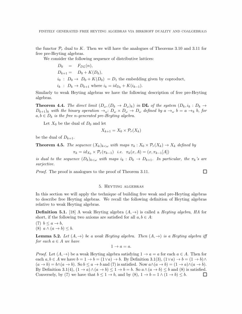
Let D be a finite distributive lattice. We have seen how to build the free weak Heytingalgebra and the free pre-Heyting algebra over D incrementally. Let FHA(D) denote the freeHA freely generated by the distributive lattice D. Further let Fn

HA(D) denote the elementsof FHA(D) of →-rank less than or equal to n. Then each Fn

HA(D) is a distributive latticeand the lattice reduct of FHA(D) is the direct limit (union) of the chain

D = F 0HA(D) ⊆ F 1

HA(D) ⊆ F 2HA(D) . . .

and the implication on FHA(D) is given by the maps →: (FnHA(D))2 → Fn+1

HA (D) with(a, b) 7→ (a → b). Further, since any Heyting algebra is a pre-Heyting algebra and theinclusion Fn

HA(D) ⊆ Fn+1HA (D) may be seen as given by the mapping a 7→ (1 → a), the

natural maps sending generators to generators make the following colimit diagrams commute

D

id��

� � i0 // K(D)

g1��

� � i1 // K(K(D))

g2��

� � i2 // . . .

D� � j0 // F 1

HA(D)� � j1 // F 2

HA(D)� � j2 // . . .

Notice that under the assignment a 7→ (1 → a), the equation (7) becomes 1 → b ≤ a → bwhich is true in any pHA by (2), and (8) becomes (1 → a) ∧ (a → b) ≤ (1 → b) which istrue in any pHA by virtue of (4). So these equations are already satisfied in the steps of theupper sequence. However, an easy calculation shows that for D the three-element lattice1 → (u → 0) and (1→ u)→ (1→ 0) are not equal (where u is the middle element) thusthe implication is not well-defined on the limit of the upper sequence. We remedy this bytaking a quotient with respect to the relational schema corresponding to

(9) 1→ (a→ b) = (1→ a)→ (1→ b)

in the second iteration of the functor K and onwards. This equation, which is a particularlytrivial family of instances of Frege’s axiom a → (b → c) = (a → b) → (a → c) is of coursetrue in intuitionistic logic but may not be of much interest there. From the algebraicperspective, this relational scheme is of course very natural as it exactly ensures that theassignment a 7→ 1 → a preserves implication. As we will see subsequently, (9) will makesure that the embedding of each element of the constructed sequence in the next in an→-homomorphism. We proceed, as we’ve done throughout this paper by identifying thedual correspondent of this equation.

Proposition 5.3. Let D be a finite distributive lattice and X its dual poset. Further, let θbe a congruence on K(K(D)). Then the following are equivalent:

(i) For all a, b ∈ D the inequality [(1 _ a) _ (1 _ b)] ≤ [1 _ (a _ b)] holds in

K(K(D))/θ;

(ii) For all x, y ∈ X the inequality [(1 _ x) _ (1 _ κ(y))] ≤ [1 _ (x _ κ(y))] holds in

K(K(D))/θ


Proof. (i) implies (ii) is clear since (ii) is a special case of (i). We prove that (ii) implies (i)(leaving out the brackets [ ] of the quotient map).

(1 _ a) _ (1 _ b) = (∨

X∋x≤a

(1 _ x)) _ (∧

X∋y�b

(1 _ κ(y)))

=∧

X∋x≤aX∋y�b

((1 _ x) _ (1 _ κ(y)))

≤∧

X∋x≤aX∋y�b

(1 _ (x _ κ(y)))

= 1 _

∧

X∋x≤aX∋y�b

(x _ κ(y))

= 1 _ (a _ b)).

We are now ready to translate this into a dual property which we will call (G) afterGhilardi who introduced it in [13].

Proposition 5.4. Let X0 be a finite poset, X1 a subposet of Pr(X0), and X2 a subposet of

Pr(X1). For i = 1, 2, let (⋆)i be the condition

x ∈ T ∈ Xi =⇒ Tx = (↓x ∩ T ) ∈ Xi

If the conditions (⋆)1 and (⋆)2 both hold then the following are equivalent:

(i) ∀x, y ∈ X0 the inequalities

[(1 _ x) _ (1 _ κ(y))] ≤ [1 _ (x _ κ(y))] hold in O(X2);

(ii) ∀τ ∈ X2 ∀T ∈ τ ∀S ∈ X1

(S ≤ T =⇒ ∃T ′ ∈ τ (T ′ ≤ T and root (S) = root (T ′)). (G)

Proof. First we prove that (i) implies (ii). To this end suppose (i) holds and let T ∈ τ ∈ X2

and S ∈ X1. Suppose that for all T′ ∈ τ either T ′ � T or root (S) 6= root (T ′). Now consider

τT = ↓T ∩ τ . By (⋆)2 we have that τT ∈ X2. Then we have root (S) 6= root (T ′) for allT ′ ∈ τT . Thus, letting x = root(S) and using the observation in Proposition 4.3, we obtain

∀T ′ ∈ τT root(T ′) 6= x

⇐⇒ ∀T ′ ∈ τT (T ′ � 1 _ x =⇒ T ′ � 1 _ κ(x))

⇐⇒ τT � (1 _ x) _ (1 _ κ(x))

=⇒ τT � 1 _ (x _ κ(x))

⇐⇒ ∀T ′ ∈ τT T ′ � x _ κ(x)

⇐⇒ ∀T ′ ∈ τT ∀y ∈ T ′ (y ≤ x =⇒ y ≤ κ(x))

⇐⇒ ∀T ′ ∈ τT x 6∈ T ′

=⇒ x 6∈ T.


The two implications come from the fact that we assume that (i) holds and because, inparticular, T ∈ τT . Now we have x = root (S) ∈ S but x 6∈ T so S � T and we have proved(ii) by contraposition.

Now suppose (ii) holds, let x, y ∈ X0, and let τ ∈ X2 such that τ � (1 _ x) _ (1 _

κ(y)). Then

τ � (1 _ x) _ (1 _ κ(y))

⇐⇒ ∀T ∈ τ (T � 1 _ x =⇒ T � 1 _ κ(y))

⇐⇒ ∀T ∈ τ (T ≤ ↓x =⇒ T ≤ ↓κ(y)).

We want to show that T � x _ κ(y) for each T ∈ τ . That is, that for all z ∈ T we havez ≤ x implies z ≤ κ(y). So let z ∈ T with z ≤ x. By (⋆)1 we have that Tz = ↓z ∩ T ∈ X1.Since Tz ≤ T it follows by (ii) that

∃T ′ ∈ τ (T ′ ≤ T and z = root (Tz) = root (T ′)).

Now x ≥ z = root (Tz) = root (T ′) implies that T ′ ≤ ↓x and thus we have T ′ ≤ ↓κ(y). Inparticular, z = root (T ′) ≤ κ(y). That is, we have shown that for all z ∈ T , if z ≤ x thenz ≤ κ(y) as required.

Our strategy in building the free n-generated Heyting algebra will be to start with D,the free n-generated distributive lattice, embed it in K(D), and then this in a quotient ofK(K(D)) obtained by quotienting out by 1 _ (a _ b) = (1 _ a) _ (1 _ b) for a, b ∈ D.For the further iterations of K this identification is iterated. The following is the generalsituation that we need to consider, viewed dually:

X0oooo root Pr(X0) oooo root

Pr(Pr(X0))

X1

� ?

OO

oooo rootPr(X1)

� ?

OO

X2

� ?

OO

We now consider the following sequence of finite posets

X0 = J(FDL(n))(= P(n))

X1 = Pr(X0)

for n ≥ 1 Xn+1 = {τ ∈ Pr(Xn) | ∀T ∈ τ ∀S ∈ Xn

(S ≤ T =⇒ ∃T ′ ∈ τ (T ′ ≤ T and root(S) = root (T ′))}.

We denote by ∇ the sequence

X0oo root X1

oo rootX2 . . .

For n ≥ 1, we say that ∇ satisfies (⋆)n if

x ∈ T ∈ Xn =⇒ Tx = (↓x ∩ T ) ∈ Xn.

Lemma 5.5. ∇ satisfies (⋆)n for each n ≥ 1 and the root maps root : Xn+1 → Xn are

surjective for each n ≥ 0.


Proof. X1 consists of all rooted subsets of X0 and thus (⋆)1 is clearly satisfied. Now letn ≥ 2. We assume that T ∈ τ ∈ Xn and we show that τT = ↓T ∩ τ also belongs to Xn. Solet U ∈ τT , S ∈ Xn and S ≤ U . Then since U ∈ τ , there exists U ′ ∈ τ such that U ′ ≤ Uand root (S) = root (U ′). But U ∈ τT implies that U ≤ T . Therefore we have U ′ ≤ T and soU ′ ∈ τT . Thus, τT ∈ Xn and ∇ satisfies (⋆)n, for each n ≥ 1. Finally, we show that all theroot maps are surjective. To see this, assume U ∈ Xn. We show that ↓U ∈ Xn+1. SupposeT ∈ ↓U and for some S ∈ Xn we have S ≤ T . Then S ∈ ↓U and by setting T ′ = S we easilysatisfy the condition (G). Finally, note that root (↓U) = U and thus root : Xn+1 → Xn issurjective.

Let ∆ be the system

D0� � i0 // D1

� � i1 // D2 . . .

of distributive lattices dual to ∇. For each n ≥ 0, in : Dn → Dn+1, is a lattice homomor-phism dual to root . By Theorem 4.2(iii) in(a) = [1 _ a]≅, for a ∈ Dn. By Lemma 5.5, rootis surjective, so each in is injective. Each Xn+1 ⊆ Pr(Xn) so that each Dn+1 is a quotientof K(Dn) and thus, for each n, we also have implication operations:

→n: Dn ×Dn → Dn+1

(a, b) 7→ [a _ b].

Here [a _ b] is the equivalence class of a _ b as an element in Dn+1. Let Dω be the limit of∆ in the category of distributive lattices then Dω is naturally turned into a Heyting algebra.

Lemma 5.6. The operations →n can be extended to an operation →ω on Dω and the algebra

(Dω,→ω) is a Heyting algebra.

Proof. The colimit Dω of ∆ may be constructed as the union of the Dns with Dn identifiedwith the image of in : Dn → Dn+1. It is then clear that the operations →n: Dn ×Dn →Dn+1 yield a total, well-defined binary operation on the limit Dω provided, for all n ∈ ωand all a, b ∈ Dn, we have in+1(→n (a, b)) =→n+1 (in(a), in(b)). But this is exactly

1→n+1 (a→n b) = (1→n a)→n+1 (1→n b).

As we’ve shown in Corollary 5.4 and Lemma 5.5, the sequence∇, and thus the dual sequence∆ have been defined exactly so that this holds. It remains to show that the algebra (Dω,→) is a Heyting algebra. Let a ∈ Dω, then there is some n ≥ 0 with a ∈ Dn. Nowa →ω a = a →n a ∈ Dn+1. Since Dn+1 is a further quotient of K(Dn) and a →n a = 1already in K(Dn), this is certainly also true in Dn+1 and 1Dn+1

= 1Dωso the equation

(1) of weak Heyting algebras is satisfied in (Dω,→ω). Similarly each of the equations (2)–(4) are satisfied in (Dω,→ω) so that it is a weak Heyting algebra. Finally, note that asin(a) = 1 →n a for each a ∈ Dn and n ∈ ω, we have a = 1 →ω a for each a ∈ Dω. ByLemma 5.2, this implies that (Dω,→ω) is a Heyting algebra.

Corollary 5.7. For each n ∈ ω, if D0 is the n-generated free distributive lattice, then

(Dω,→ω) constructed above is the n-generated free Heyting algebra.

Proof. Let FHA(n) denote the free HA freely generated by n generators. This is of coursethe same as the free HA generated by D, FHA(D), where D is the free distributive latticegenerated by n elements. As discussed at the beginning of this section this lattice is thecolimit (union) of the chain

D = F 0HA(D) ⊆ F 1

HA(D) ⊆ F 2HA(D) . . .


and the implication on FHA(D) is given by the maps →: (FnHA(D))2 → Fn+1

HA (D) with(a, b) 7→ (a → b). Further, the natural maps sending generators to generators make thefollowing colimit diagrams commute

D

id��

� � // K(D)

��

� � // K(K(D))

��

� � // . . .

D� � j0 // F 1

HA(D)� � j1 // F 2

HA(D)� � j2 // . . .

Now, the system ∆ is obtained from the upper sequence by quotienting out by the equations1→n+1 (a→n b) = (1→n a)→n+1 (1→n b) for each n ≥ 0. Since these equations all holdfor the lower sequence, it follows that the Dns are intermediate quotients:

D

id��

� � // K(D)

��

� � // K(K(D))

��

� � // . . .

D0

id��

� � i0 // D1

��

� � i1 // D2

��

� � i2 // . . .

D� � j0 // F 1

HA(D) � � j1 // F 2HA(D) � � j2 // . . .

Therefore, FHA(n) is a homomorphic image of Dω. Moreover, any map f : n → B with

B a Heyting algebra defines a unique extension f : FHA(n) → B such that f ◦ i = f ,where i : n→ FHA(n) is the injection of the free generators. Since i actually maps into thesublattice of FHA(n) generated by n, which is the initial lattice D = D0 in our sequences,

composition of f with the quotient map from Dω to FHA(n) shows that Dω also has theuniversal mapping property (without the uniqueness). The uniqueness follows since Dω

clearly is generated by n as HA (since D0 is generated by n as a lattice, D1 is generated byD0 using →0, and so on). Since the free HA on n generators is unique up to isomorphismand Dω has its universal mapping property and is a Heyting algebra, it follows it is the freeHA (and the quotient map from Dω to FHA(n) is in fact an isomorphism).

6. A coalgebraic representation of wHAs and PHAs

In this section we discuss coalgebraic semantics for weak and pre-Heyting algebras. Acoalgebraic representation of modal algebras and distributive modal algebras can be foundin [1], [19] and [23], [8], respectively.

We recall that a Stone space is a compact Hausdorff space with a basis of clopen sets.For a Stone space X, its Vietoris space V (X) is defined as the set of all closed subsets ofX, endowed with the topology generated by the subbasis

(1) �U = {F ∈ V (X) : F ⊆ U},(2) ♦U = {F ∈ V (X) : F ∩ U 6= ∅},

where U ranges over all clopen subsets of X. It is well known that X is a Stone space iffV (X) is a Stone space. Let X and X ′ be Stone spaces and f : X → X ′ be a continuousmap. Then V (f) = f [ ] is a continuous map between V (X) and V (X ′). We denote byV the functor on Stone spaces that maps every Stone space X to its Vietoris space V (X)


and maps every continuous map f to V (f). Every modal algebra (B,�) corresponds to acoalgebra (X,α : X → V X) for the Vietoris functor on Stone spaces [1, 19]. Coalgebrascorresponding to distributive modal algebras are described in [23] and [8]. We note thatmodal algebras as well as distributive modal algebras are given by rank 1 axioms. Usingthe same technique as in Section 3, one can obtain a description of free modal algebras andfree distributive modal algebras [1], [14], [8].

Our goal is to characterize coalgebras corresponding to weak Heyting algebras and pre-Heyting algebras. Recall that a Priestley space is a pair (X,≤) where X is a Stone spaceand ≤ is a reflexive, antisymmetric and transitive relation satisfying the Priestley separation

axiom:

If x, y ∈ X are such that x 6≤ y, then there exists a clopen downset Uwith y ∈ U and x /∈ U .

We denote by PS the category of Priestley spaces and order-preserving continuous maps. Itis well known that every distributive lattice D can be represented as a lattice of all clopendownsets of the Priestley space of its prime filters. Given a Priestley space X, let Vr(X) bea subspace of V (X) of all closed rooted subsets of X. The same proof as for V (X) showsthat Vr(X) is a Stone space.

Lemma 6.1. Let X be a Priestley space. Then

(1) (V (X),⊆) is a Priestley space.

(2) (Vr(X),⊆) is a Priestley space.

Proof. (1) As we mentioned above V (X) is a Stone space. Let F,F ′ ∈ V (X) and F 6⊆ F ′.Then there exists x ∈ F such that x /∈ F ′. Since every compact Hausdorff space is normal,there exists a clopen set U such that F ′ ⊆ U and x /∈ U . Thus, F ′ ∈ �U and F /∈ �U . Allwe need to observe now is that for each clopen U of X, the set �U is a clopen ⊆-downsetof V (X). But this is obvious.

The proof of (2) is the same as for (1).

Let (X,≤) and (X ′,≤′) be Priestley spaces and f : X → X ′ a continuous order-preservingmap. Then it is easy to check that V (f) = f [ ] is a continuous order-preserving map between(V (X),⊆) and (V (X ′),⊆), and Vr(f) = f [ ] is a continuous order-preserving map between(Vr(X),⊆) and (Vr(X

′),⊆). Thus, V and Vr define functors on the category of Priestleyspaces.

Definition 6.2. (Celani and Jansana [11]) A weak Heyting space is a triple (X,≤, R) suchthat (X,≤) is a Priestley space and R is a binary relation on X satisfying the followingconditions:

(1) R(x) = {y ∈ X : xRy} is a closed set, for each x ∈ X.(2) For each x, y, z ∈ X if x ≤ y and xRz, then yRz.(3) For each clopen set U ⊆ X the sets [R](U) = {x ∈ X : R(x) ⊆ U} and 〈R〉(U) = {x ∈

U : R(x) ∩ U 6= ∅} are clopen.

Let (X,≤, R) and (X ′,≤′, R′) be two weak Heyting spaces. We say that f : X → X ′ isa weak Heyting morphism if f is continuous, ≤-preserving and R-bounded morphism (i.e.,for each x ∈ X we have fR(x) = R′f(x)). Then the category of weak Heyting algebras isdually equivalent to the category of weak Heyting spaces and weak Heyting morphisms [11].We will quickly recall how the dual functors are defined on objects. Given a weak Heytingalgebra (A,→) we take a Priestley dual XA of A and define RA on XA by setting: for each


x, y ∈ XA, xRAy if for each a, b ∈ A, a → b ∈ x and b ∈ x imply b ∈ y. Conversely, if(X,≤, R) is a weak Heyting space, then we take the distributive lattice of all clopen downsetsof X and for clopen downsets U, V ⊆ X we define U → V = {x ∈ X : R(x) ∩ U ⊆ V }.

Remark 6.3. In fact, Celani and Jansana [11] work with clopen upsets instead of downsetsand the inverse of the relation R. We chose working with downsets to be consistent withthe previous parts of this paper.

Theorem 6.4. The category of weak Heyting spaces is isomorphic to the category of Vietoris

coalgebras on the category of Priestley spaces.

Proof. Given a weak Heyting space (X,≤, R). We consider a coalgebra (X,R(.) : X →V (X)). The map R(.) is well defined by Definition 6.2(1). It is order-preserving by Def-inition 6.2(2) and is continuous by Definition 6.2(3). Thus, (X,R(.) : X → V (X)) is aV -coalgebra. Conversely, let (X,α : X → V (X)) be a V -coalgebra. Then (X,Rα), wherexRαy iff y ∈ α(x), is a weak Heyting space. Indeed, R being well defined and order-preserving imply conditions (1) and (2) of Definition 6.2, respectively. Finally, α beingcontinuous implies condition (3) of Definition 6.2. That this correspondence can be liftedto the isomorphism of categories is easy to check.

We say that a weakly Heyting space (X,≤, R) is a pre-Heyting space if for each x ∈ Xthe set R(x) is rooted.

Theorem 6.5.

(1) The category of pre-Heyting algebras is dually equivalent to the category of pre-Heyting

spaces.

(2) The category of pre-Heyting spaces is isomorphic to the category of Vr-coalgebras on

the category of Priestley spaces.

Proof. (1) By the duality of weak Heyting algebras and weak Heyting spaces it is sufficientto show that a weak Heyting algebra satisfies conditions (5)–(6) of Definition 4.1 iff R(x)is rooted. We will show, as in Theorem 4.2, that the axiom (5) is equivalent to R(x) 6= ∅,for each x ∈ X, while axiom (6) is equivalent to R(x) having a unique maximal element.Assume that a weak Heyting space (X,≤, R) validates axiom (5). Then in the weak Heytingalgebra of all clopen downsets of X we have X → ∅ = ∅. Thus for each x ∈ X we haveR(x) ⊆ ∅ iff x ∈ ∅. Thus, for each x ∈ X we have R(x) 6= ∅. Now suppose for each clopendownsets U, V ⊆ X the following holds X → (U ∪V ) ⊆ (X → U)∪(X → V ). Then we havethat R(x) ⊆ U∪V implies R(x) ⊆ U or R(x) ⊆ V . Since R(x) is closed and X is a Priestleyspace, we have that every point of R(x) is below some maximal point of R(x). We assumethat there exists more than one maximal point of R(x). Then the same argument as in [5,Theorem 2.7(a)] shows that there are clopen downsets U and V such that R(x) ⊆ U ∪ V ,but R(x) 6⊆ U , R(x) 6⊆ V . This is a contradiction, so R(x) is rooted. On the other hand, itis easy to check that if R(x) is rooted for each x ∈ X, then (5) and (6) are valid. Finally, aroutine verification shows that this correspondence can be lifted to an isomorphism of thecategories of pre-Heyting algebras and pre-Heyting spaces.

The proof of (2) is similar to the proof of Theorem 6.4. The extra condition on pre-Heyting spaces obviously implies that a mapR(.) : X → Vr(X) is well defined and conversely(X,α : X → Vr(X)) being a coalgebra implies that Rα(x) is rooted for each x ∈ X. Therest of the proof is a routine check.


Thus, we obtained a coalgebraic semantics/representation of weak and pre-Heytingalgebras.

7. Conclusions and future work

In this paper we described finitely generated free (weak, pre-) Heyting algebras using aninitial algebra-like construction. The main idea is to split the axiomatization of Heytingalgebras into its rank 1 and non-rank 1 parts. The rank 1 approximants of Heyting algebrasare weak and pre-Heyting algebras. For weak and pre-Heyting algebras we applied thestandard initial algebra construction and then adjusted it for Heyting algebras. We usedBirkhoff duality for finite distributive lattices and finite posets to obtain the dual charac-terization of the finite posets that approximate the duals of free algebras. As a result, weobtained Ghilardi’s representation of these posets in a systematic and modular way. Wealso gave a coalgebraic representation of weak and pre-Heyting algebras.

There are a few possible directions for further research. As we mentioned in the intro-duction, although we considered Heyting algebras (intuitionistic logic), this method couldbe applied to other non-classical logics. More precisely, the method is available if a signatureof the algebras for this logic can be obtained by adding an extra operator to a locally finitevariety. Thus, various non-rank 1 modal logics such as S4, K4 and other more compli-cated modal logics, as well as distributive modal logics, are the obvious candidates. On theother hand, one cannot always expect to have such a simple representation of free algebras.The algebras corresponding to other many-valued logics such as MV -algebras, l-groups,BCK-algebras and so on, are other examples where this method could lead to interestingrepresentations. The recent work [9] that connects ontologies with free distributive algebraswith operators shows that such representations of free algebras are not only interesting froma theoretical point of view, but could have very concrete applications.

Acknowledgements The first listed author would like to thank Mamuka Jibladze andDito Pataraia for many interesting discussions on the subject of the paper. The authors arealso very grateful to the anonymous referees for many helpful suggestions that substantiallyimproved the presentation of the paper.

References

[1] S. Abramsky. A Cook’s tour of the finitary non-well-founded sets. In S. A. et al., editor, We Will ShowThem: Essays in honour of Dov Gabbay, pages 1–18. College Publications, 2005.

[2] J. Adamek and V. Trnkova. Automata and algebras in categories, volume 37 of Mathematics and itsApplications (East European Series). Kluwer, Dordrecht, 1990.

[3] S. Aguzzoli, B. Gerla, and V. Marra. Godel algebras free over finite distributive lattices. Annals of Pureand Applied Logic, 155(3):183–193, 2008.

[4] F. Bellissima. Finitely generated free Heyting algebras. J. Symbolic Logic, 51(1):152–165, 1986.[5] G. Bezhanishvili and N. Bezhanishvili. Profinite Heyting algebras. Order, 25(3):211–223, 2008.[6] N. Bezhanishvili. Lattices of Intermediate and Cylindric Modal Logics. PhD thesis, University of Ams-

terdam, 2006.[7] N. Bezhanishvili and M. Gehrke. Free Heyting algebras: revisited. In CALCO 2009, volume 5728 of

LNCS, pages 251–266. Springer-Verlag, 2009.[8] N. Bezhanishvili and A. Kurz. Free modal algebras: A coalgebraic perspective. In CALCO 2007, volume

4624 of LNCS, pages 143–157. Springer-Verlag, 2007.[9] H. Bruun, D. Coumans, and M. Gehrke. Distributive lattice-structured ontologies. In CALCO 2009,

volume 5728 of LNCS, pages 267–283. Springer-Verlag, 2009.


[10] C. Butz. Finitely presented Heyting algebras. Technical report, BRICS, Arhus, 1998.[11] S. Celani and R. Jansana. Bounded distributive lattices with strict implication. Math. Log. Q.,

51(3):219–246, 2005.[12] A. Chagrov and M. Zakharyaschev. Modal Logic. The Clarendon Press, 1997.[13] S. Ghilardi. Free Heyting algebras as bi-Heyting algebras. Math. Rep. Acad. Sci. Canada XVI., 6:240–

244, 1992.[14] S. Ghilardi. An algebraic theory of normal forms. Annals of Pure and Applied Logic, 71:189–245, 1995.[15] S. Ghilardi. Continuity, freeness, and filtrations. Technical report, Universita DegliStudi di Milano,

2010. Available at http://homes.dsi.unimi.it/ ghilardi/allegati/research.html.[16] S. Ghilardi and M. Zawadowski. Sheaves, Games and Model Completions. Kluwer, 2002.[17] R. Grigolia. Free algebras of non-classical logics. “Metsniereba”, Tbilisi, 1987. (in Russian).[18] P. T. Johnstone. Stone spaces. Cambridge University Press, Cambridge, 1982.[19] C. Kupke, A. Kurz, and Y. Venema. Stone coalgebras. Theoretical Computer Science, 327(1-2):109–134,

2004.[20] A. Kurz and J. Rosicky. The Goldblatt-Thomason theorem for coalgebras. In CALCO 2007, volume

4624 of LNCS, pages 342–355. Springer-Verlag, 2007.[21] A. Nerode. Some Stone spaces and recursion theory. Duke Math. J., 26:397–406, 1959.[22] I. Nishimura. On formulas of one variable in intuitionistic propositional calculus. J. Symbolic Logic,

25:327–331, 1960.[23] A. Palmigiano. A coalgebraic view on positive modal logic. Theoretical Computer Sceince, 327:175–195,

2004.[24] D. Pataraia. High order cylindric algebras. 2011. In preparation.[25] D. Pattinson and L. Schroder. Beyond rank 1: Algebraic semantics and finite models for coalgebraic

logics. In FOSSACS 2008, volume 4962 of LNCS, pages 66–80. Springer, 2008.[26] L. Rieger. On the lattice theory of Brouwerian propositional logic. Acta Fac. Nat. Univ. Carol., Prague,

189:1–40, 1949.[27] V. Rybakov. Rules of inference with parameters for intuitionistic logic. J. Symbolic Logic, 57(3):912–923,

1992.[28] L. Schroder and D. Pattinson. PSPACE bounds for rank-1 modal logics. In Proc. 21st IEEE Symposium

on Logic in Computer Science (LICS 2006), pages 231–242, 2006.[29] V. Shehtman. Rieger-Nishimura ladders. Dokl. Akad. Nauk SSSR, 241(6):1288–1291, 1978.[30] A. Urquhart. Free Heyting algebras. Algebras Universalis, 3:94–97, 1973.[31] Y. Venema. Algebras and coalgebras. In P. Blackburn, J. van Benthem, and F. Wolter, editors, Handbook

of Modal Logic, pages 331–426. Elsevier, 2007.[32] P. Whitman. Splittings of a lattice. Amer. J. Math., 65:179–196, 1943.

This work is licensed under the Creative Commons Attribution-NoDerivs License. To viewa copy of this license, visit http://creativecommons.org/licenses/by-nd/2.0/ or send aletter to Creative Commons, 171 Second St, Suite 300, San Francisco, CA 94105, USA, orEisenacher Strasse 2, 10777 Berlin, Germany

Documents

FINITELY GENERATED FREE HEYTING ALGEBRAS VIA BIRKHOFF ... · FINITELY GENERATED FREE HEYTING ALGEBRAS VIA BIRKHOFF ... algebra is built on a distributive lattice step-by ... FINITELY