Embed Size (px)
Citation preview

Draft Appendix C: AMHS Regression Models
Prepared for
Alaska Department of Transportation and Public Facilities
January 2020 Prepared by

Preparers Team Member Project Role Michael Fisher Project Manager Marcus Hartley Principal Investigator Brock Lane Analyst Emilie Franke Analyst Terri McCoy Editor
Please cite as: Northern Economics, Inc. Draft Appendix C: AMHS Regression Models. Prepared for Alaska Department of Transportation and Public Facilities. January 2020.

i
Contents
Section Page
1 Introduction and Methods ......................................................................................................... 1
2 Regression Models .................................................................................................................... 5
Table Page
Table 1. Indicator Variable Coding ..................................................................................................... 2 Table 2. Summary of AMHS Regression Models ................................................................................. 3 Table 3. Mainline (All) Regression Models and Baseline Values ........................................................... 5 Table 4. Mainline Excluding Bellingham Regression Models and Baseline Values ................................ 6 Table 5. Mainline Excluding Prince Rupert Regression Models and Baseline Values ............................ 7 Table 6. Mainline Excluding Bellingham and Prince Rupert Regression Models and Baseline Values ... 8 Table 7. SE Feeder, To or From is Juneau Regression Models and Baseline Values .............................. 9 Table 8. SE Feeder, To or From is Sitka Regression Models and Baseline Values ............................... 10 Table 9. Lynn Canal, To or From is Juneau Regression Models and Baseline Values .......................... 11 Table 10. PWS for Cordova-Whittier and Whitter-Cordova Port-Pairs Regression Models and
Baseline Values ......................................................................................................................... 12 Table 11. Hom-Kod for Homer-Kodiak and Kodiak-Homer Port-Pairs Regression Models and
Baseline Values ......................................................................................................................... 13 Table 12. SW, To or From is Homer Regression Models and Baseline Values ................................... 14 Table 13. SW, To or From is Kodiak Regression Models and Baseline Values .................................... 15 Table 14. Metlakatla-Ketchikan and Ketchikan-Metlakatla Port-Pairs Regression Models and
Baseline Values ......................................................................................................................... 16 Table 15. PWS for Whittier-Valdez and Valdez-Whitter Port-Pairs Regression Models and Baseline
Values ....................................................................................................................................... 17 Table 16. Lynn Canal for Haines-Skagway and Skagway-Haines Port-Pairs Regression Models and
Baseline Values ......................................................................................................................... 18 Table 17. Cross Gulf for Service to Chenega Bay, Ouzinkie, Port Lions, and Seldovia Regression
Models and Baseline Values ...................................................................................................... 19 Table 18. Cross Gulf for Service to Chenega Bay, Ouzinkie, Port Lions, and Seldovia, When To or
From is Not Bellingham Regression Models and Baseline Values ................................................ 20
Figure Page
Figure 1. Sample of AMHS Regression Model Data ............................................................................ 1 Equation Page
Equation 1. Mainline (All) Regression Model Equations ...................................................................... 5 Equation 2. Mainline Excluding Bellingham Regression Model Equations ............................................ 6 Equation 3. Mainline Excluding Prince Rupert Regression Model Equations ........................................ 7 Equation 4. Mainline Excluding Bellingham and Prince Rupert Regression Model Equations ............... 8

Draft Appendix C: AMHS Regression Models
ii
Equation 5. SE Feeder, To or From is Juneau Regression Model Equations .......................................... 8 Equation 6. SE Feeder, To or From is Sitka Regression Model Equations ........................................... 10 Equation 7. Lynn Canal, To or From is Juneau Regression Model Equations ...................................... 11 Equation 8. PWS for Cordova-Whittier and Whitter-Cordova Port-Pairs Regression Model
Equations .................................................................................................................................. 12 Equation 9. Hom-Kod for Homer-Kodiak and Kodiak-Homer Port-Pairs Regression Model
Equations .................................................................................................................................. 13 Equation 10. SW, To or From is Homer Regression Model Equations ............................................... 14 Equation 11. SW, To or From is Kodiak Regression Model Equations ................................................ 15 Equation 12. Metlakatla-Ketchikan and Ketchikan-Metlakatla Port-Pairs Regression Model
Equations .................................................................................................................................. 16 Equation 13. PWS for Whittier-Valdez and Valdez-Whitter Port-Pairs Regression Model Equations ... 17 Equation 14. Lynn Canal for Haines-Skagway and Skagway-Haines Port-Pairs Regression Model
Equations .................................................................................................................................. 18 Equation 16. Cross Gulf for Service to Chenega Bay, Ouzinkie, Port Lions, and Seldovia Equations .. 19 Equation 17. Cross Gulf for Service to Chenega Bay, Ouzinkie, Port Lions, and Seldovia, When
To or From is Not Bellingham Equations .................................................................................... 20

1
1 Introduction and Methods The purpose of this appendix is to summarize the regression models which serve as a basis for the AMHS reshaping study revenue models. Regression models are a statistical method of analyzing data that are used for predictions and forecasting in a variety of industries. Regression modeling uses actual data to create an equation which isolates the effects of variables on a specific variable of interest, the dependent variable. In the case of AMHS data, the study team estimates the number of passengers onboard a vessel or the combined length of vehicles on the car deck (dependent variables) as a function of other important independent variables including time of year, services available at the departure and arrival ports, number of sailings, and fare prices.
Regression models provide a standardized way to estimate revenues for different combinations of assumptions. Since each model is derived from historical travel patterns, they provide a mathematical and objective basis for comparing each set of conditions. This study compares several quantitative assessments with unique AMHS schedules, levels of service, and operating parameters; however, each assessment relies on the same underlying data and model structure as the basis for revenue estimates.
The mathematical models presented in this appendix use an ordinary-least-squares estimation method1 to perform the regression, which was completed using the statistical analysis software STATA (version 12). The regression models are derived from vessel data provided by DOT&PF. The data were reorganized into the structure shown in Figure 1 below, where each row represents one month in a given year, and a unique pair of AMHS port cities. For each year-month and city-pair combination, the data summarizes vessel and revenue characteristics such as the number of sailings performed, the number of passengers, cabin rentals, and car deck occupancy, as well as the revenues collected for each.
Figure 1. Sample of AMHS Regression Model Data
The model compares all points in the data set (July 2008–December 2019) to estimate how much the dependent variable is affected by each independent variable. The model uses the data to recognize that sailings during summer months will have more passengers and vehicles than during winter months. Similarly, the models use historical changes in key variables, like prices and the level of AMHS service, to allow the study team to make predictions based on changes to those variables.
In addition to the vessel data, the regression models account for several exogenous traits that are specific to AMHS port cities. Ridership on AMHS trips will likely be higher when either the departure or arrival city has important transportation infrastructure or services, which are treated as indicator or “dummy” variables—those that take a value of either 1 or 0 in the data set. Table 1 shows the
1 Ordinary Least Squares is a common linear regression model that estimates the effects from an explanatory set of variables on the dependent variable. The model is based on minimizing the sum of squares of the differences between the observed and model-predicted dependent variable values. The difference between the actual and predicted values is also called a residual value.

Draft Appendix C: AMHS Regression Models
2
indicator variable values for each city to account for the presence of hospitals, access to a contiguous road system head, access to a major metro area to account for grocery and major retail stores, access to a jet service airport, and an additional indicator if the city is considered a regional hub.
Table 1. Indicator Variable Coding
Area Name Has Hospital? Has
Roadhead? Access Major Metro Area?
Jet Service Airport? Regional Hub?
Akutan city 0 0 0 0 0 Cold Bay city 0 0 0 1 0 False Pass city 0 0 0 0 0 King Cove city 0 0 0 0 0 Sand Point city 0 0 0 0 0 Unalaska city 0 0 0 0 1 Haines CDP 0 1 0 0 0 Angoon city 0 0 0 0 0 Gustavus city 0 0 0 0 0 Hoonah city 0 0 0 0 0 Pelican city 0 0 0 0 0 Tenakee Springs city 0 0 0 0 0 Juneau city and borough place 1 0 0 1 1 Homer city 0 1 1 1 1 Seldovia city 0 0 0 0 0 Ketchikan city 1 0 0 1 1 Kodiak city 1 0 0 1 1 Old Harbor city 0 0 0 0 0 Ouzinkie city 0 0 0 0 0 Port Lions city 0 0 0 0 0 Chignik city 0 0 0 0 0 Petersburg city 0 0 0 0 0 Kake city 0 0 0 0 0 Metlakatla CDP 0 0 0 0 0 Sitka city and borough place 1 0 0 1 1 Skagway CDP 0 1 0 0 0 Chenega CDP 0 0 0 0 0 Cordova city 0 0 0 1 0 Tatitlek CDP 0 0 0 0 0 Valdez city 1 1 0 0 0 Whittier city 0 1 1 0 1 Wrangell city and borough place 0 0 0 0 0 Yakutat CDP 0 0 0 1 0 Prince Rupert, BC 1 1 0 1 Bellingham, WA 1 1 1 0 1 Annette Bay 0 0 0 0 0
Draft Appendix C: AMHS Regression Models
3
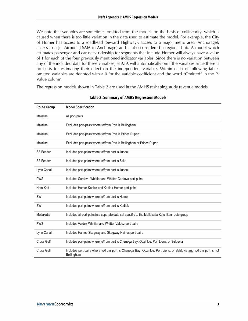
We note that variables are sometimes omitted from the models on the basis of collinearity, which is caused when there is too little variation in the data used to estimate the model. For example, the City of Homer has access to a roadhead (Seward Highway), access to a major metro area (Anchorage), access to a Jet Airport (TSAIA in Anchorage) and is also considered a regional hub. A model which estimates passenger and car deck ridership for segments that include Homer will always have a value of 1 for each of the four previously mentioned indicator variables. Since there is no variation between any of the included data for these variables, STATA will automatically omit the variables since there is no basis for estimating their effect on the independent variable. Within each of following tables omitted variables are denoted with a 0 for the variable coefficient and the word “Omitted” in the P-Value column.
The regression models shown in Table 2 are used in the AMHS reshaping study revenue models.
Table 2. Summary of AMHS Regression Models
Route Group Model Specification
Mainline All port-pairs
Mainline Excludes port-pairs where to/from Port is Bellingham
Mainline Excludes port-pairs where to/from Port is Prince Rupert
Mainline Excludes port-pairs where to/from Port is Bellingham or Prince Rupert
SE Feeder Includes port-pairs where to/from port is Juneau
SE Feeder Includes port-pairs where to/from port is Sitka
Lynn Canal Includes port-pairs where to/from port is Juneau
PWS Includes Cordova-Whittier and Whitter-Cordova port-pairs
Hom-Kod Includes Homer-Kodiak and Kodiak-Homer port-pairs
SW Includes port-pairs where to/from port is Homer
SW Includes port-pairs where to/from port is Kodiak
Metlakatla Includes all port-pairs in a separate data set specific to the Metlakatla-Ketchikan route group
PWS Includes Valdez-Whittier and Whitter-Valdez port-pairs
Lynn Canal Includes Haines-Skagway and Skagway-Haines port-pairs
Cross Gulf Includes port-pairs where to/from port is Chenega Bay, Ouzinkie, Port Lions, or Seldovia
Cross Gulf Includes port-pairs where to/from port is Chenega Bay, Ouzinkie, Port Lions, or Seldovia and to/from port is not Bellingham

Draft Appendix C: AMHS Regression Models
4
For each model specification the study team constructed two regressions: one to predict passenger ridership and one to predict car deck ridership. These models are presented in a single table for each model specification, and show the variable coefficients as well as their statistical significance, using a P-value2. Model goodness-of-fit is measured using an R-squared value3, provided at the bottom of each table along with the number of included observations from the data set. Each table is also preceded by an equation form of the regression models. The key variables in the models are the number of monthly sailings and the fare price paid by travelers. Additional model parameters are used in model estimation to account for seasonality and characteristics of individual ports.
2 A P-value is the output of a statistical significance test called a Z-test which compares the mean value of two approximately normal distributions. In a regression, the Z-test compares data observations with differing independent variable values to measure the importance of the variable in explaining differences in the observed data. The P-value represents the likelihood or probability that the coefficient estimate for a variable is not statistically significant or important to the model. A P-value of 10 percent or less is widely accepted in econometric models and means that there is a 90 percent or greater chance that the variable is statistically significant.
3 An R-squared value is a common measurement of model goodness-of-fit and provides an indication of model accuracy. A model with an R-squared value of 1.00 or 100 percent is one whose independent variable coefficients and equation perfectly explain all changes in the dependent variable within the data set. Declining R-squared values, measured as a percentage, indicate declining model accuracy and quality. For example, a model with an R-Squared value of 0.5 explains 50 percent of the observed variation in the dependent variable. The remaining 50 percent can be due to factors not accounted for in the model or random error in the residual values.

Draft Appendix C: AMHS Regression Models
5
2 Regression Models
Equation 1. Mainline (All) Regression Model Equations
𝑌𝑌𝑃𝑃𝑃𝑃𝑃𝑃𝑃𝑃𝑃𝑃𝑃𝑃𝑃𝑃𝑃𝑃𝑃𝑃𝑃𝑃 𝑝𝑝𝑃𝑃𝑃𝑃 𝑆𝑆𝑃𝑃𝑆𝑆𝑆𝑆𝑆𝑆𝑃𝑃𝑃𝑃 = 0.9 + 0.39 ∙ 𝑀𝑀𝑀𝑀 − 5.29 ∙ 𝐹𝐹𝐹𝐹𝑃𝑃𝑃𝑃𝑃𝑃𝑃𝑃𝑃𝑃𝑃𝑃𝑃𝑃𝑃𝑃𝑃𝑃𝑃𝑃 + 6.79 ∙ 𝐹𝐹𝑀𝑀 − 2.37 ∙ 𝑊𝑊𝑀𝑀 + �𝛽𝛽𝑆𝑆 ∙ 𝐹𝐹𝑃𝑃𝑃𝑃𝑃𝑃𝑃𝑃𝑃𝑃𝑃𝑃𝑃𝑃𝑃𝑃𝑆𝑆
5
𝑆𝑆=1
𝑌𝑌𝐶𝐶𝑃𝑃𝑃𝑃 𝐷𝐷𝑃𝑃𝐷𝐷𝐷𝐷 𝑝𝑝𝑃𝑃𝑃𝑃 𝑆𝑆𝑃𝑃𝑆𝑆𝑆𝑆𝑆𝑆𝑃𝑃𝑃𝑃 = −13.22 + 1.80 ∙ 𝑀𝑀𝑀𝑀 − 46.99 ∙ 𝐹𝐹𝐹𝐹𝐶𝐶𝑃𝑃𝑃𝑃𝐷𝐷𝑃𝑃𝐷𝐷𝐷𝐷 + 22.22 ∙ 𝐹𝐹𝑀𝑀 − 21.89 ∙ 𝑊𝑊𝑀𝑀 + �𝛽𝛽𝑆𝑆 ∙ 𝐹𝐹𝑃𝑃𝑃𝑃𝑃𝑃𝑃𝑃𝑃𝑃𝑃𝑃𝑃𝑃𝑃𝑃𝑆𝑆
5
𝑆𝑆=1
Table 3. Mainline (All) Regression Models and Baseline Values
Variable Type Abbreviation Variable Name Passengers per Sailing Car Deck (feet) per Sailing
Coefficient (β) P-Value Coefficient (β) P-Value Key Variables
N/A N/A Constant 0.90 0.29 -13.22 0.09
Continuous MS Monthly Sailings 0.39 0.00 1.80 0
Continuous FP Fare Price -5.29 0.00 -46.99 0.56
Indicator Variable PM Peak Months 6.79 0.00 22.22 0
Indicator Variable WM Winter Months -2.37 0.00 -21.89 0 Parameters for Model Specification
Indicator Variable i=1 Has a Hospital? 2.19 0.00 5.37 0.221
Indicator Variable i=2 Has Road Head? -0.26 0.53 31.27 0
Indicator Variable i=3 Access Metro Area? 21.45 0.00 183.42 0
Indicator Variable i=4 Has Jet Airport? 8.43 0.00 80.21 0
Indicator Variable i=5 Is Regional Hub? 0.00 (Omitted) 0.00 (Omitted)
Observations 9,301 9,301 R-Squared 0.29 0.31
*Note: Peak Months and Winter Months variables are used as indicator variables within the regression, but percentage values of operating months within the modeled schedule are used as the input within the revenue model.

Draft Appendix C: AMHS Regression Models
6
Equation 2. Mainline Excluding Bellingham Regression Model Equations
𝑌𝑌𝑃𝑃𝑃𝑃𝑃𝑃𝑃𝑃𝑃𝑃𝑃𝑃𝑃𝑃𝑃𝑃𝑃𝑃𝑃𝑃 𝑝𝑝𝑃𝑃𝑃𝑃 𝑆𝑆𝑃𝑃𝑆𝑆𝑆𝑆𝑆𝑆𝑃𝑃𝑃𝑃 = −0.24 + 0.43 ∙ 𝑀𝑀𝑀𝑀 − 1.63 ∙ 𝐹𝐹𝐹𝐹𝑃𝑃𝑃𝑃𝑃𝑃𝑃𝑃𝑃𝑃𝑃𝑃𝑃𝑃𝑃𝑃𝑃𝑃𝑃𝑃 + 3.93 ∙ 𝐹𝐹𝑀𝑀 − 0.98 ∙ 𝑊𝑊𝑀𝑀 + �𝛽𝛽𝑆𝑆 ∙ 𝐹𝐹𝑃𝑃𝑃𝑃𝑃𝑃𝑃𝑃𝑃𝑃𝑃𝑃𝑃𝑃𝑃𝑃𝑆𝑆
5
𝑆𝑆=1
𝑌𝑌𝐶𝐶𝑃𝑃𝑃𝑃 𝐷𝐷𝑃𝑃𝐷𝐷𝐷𝐷 𝑝𝑝𝑃𝑃𝑃𝑃 𝑆𝑆𝑃𝑃𝑆𝑆𝑆𝑆𝑆𝑆𝑃𝑃𝑃𝑃 = −7.08 + 1.79 ∙ 𝑀𝑀𝑀𝑀 − 18.72 ∙ 𝐹𝐹𝐹𝐹𝐶𝐶𝑃𝑃𝑃𝑃𝐷𝐷𝑃𝑃𝐷𝐷𝐷𝐷 + 14.76 ∙ 𝐹𝐹𝑀𝑀 − 18.38 ∙ 𝑊𝑊𝑀𝑀 + �𝛽𝛽𝑆𝑆 ∙ 𝐹𝐹𝑃𝑃𝑃𝑃𝑃𝑃𝑃𝑃𝑃𝑃𝑃𝑃𝑃𝑃𝑃𝑃𝑆𝑆
5
𝑆𝑆=1
Table 4. Mainline Excluding Bellingham Regression Models and Baseline Values
Variable Type Abbreviation Variable Name Passengers per Sailing Car Deck (feet) per Sailing
Coefficient (β) P-Value Coefficient (β) P-Value Key Variables
N/A N/A Constant -0.24 0.74 -7.08 0.23
Continuous MS Monthly Sailings 0.43 0.00 1.79 0.00
Continuous FP Fare Price -1.63 0.17 -18.72 0.76
Indicator Variable PM Peak Months 3.93 0.00 14.76 0.00
Indicator Variable WM Winter Months -0.98 0.01 -18.38 0.00
Parameters for Model Specification
Indicator Variable i=1 Has a Hospital? 5.86 0.00 37.08 0.00
Indicator Variable i=2 Has Road Head? -1.33 0.00 18.56 0.00
Indicator Variable i=3 Access Metro Area? 0.00 (Omitted) 0.00 (Omitted)
Indicator Variable i=4 Has Jet Airport? 4.11 0.00 39.06 0.00
Indicator Variable i=5 Is Regional Hub? 0.00 (Omitted) 0.00 (Omitted)
Observations 7,590 7,590 R-Squared 0.18 0.15
*Note: Peak Months and Winter Months variables are used as indicator variables within the regression, but percentage values are used as the input within the revenue model equations.

Draft Appendix C: AMHS Regression Models
7
Equation 3. Mainline Excluding Prince Rupert Regression Model Equations
𝑌𝑌𝑃𝑃𝑃𝑃𝑃𝑃𝑃𝑃𝑃𝑃𝑃𝑃𝑃𝑃𝑃𝑃𝑃𝑃𝑃𝑃 𝑝𝑝𝑃𝑃𝑃𝑃 𝑆𝑆𝑃𝑃𝑆𝑆𝑆𝑆𝑆𝑆𝑃𝑃𝑃𝑃 = 9.69 + 0.50 ∙ 𝑀𝑀𝑀𝑀 − 19.77 ∙ 𝐹𝐹𝐹𝐹𝑃𝑃𝑃𝑃𝑃𝑃𝑃𝑃𝑃𝑃𝑃𝑃𝑃𝑃𝑃𝑃𝑃𝑃𝑃𝑃 + 5.89 ∙ 𝐹𝐹𝑀𝑀 − 2.33 ∙ 𝑊𝑊𝑀𝑀 + �𝛽𝛽𝑆𝑆 ∙ 𝐹𝐹𝑃𝑃𝑃𝑃𝑃𝑃𝑃𝑃𝑃𝑃𝑃𝑃𝑃𝑃𝑃𝑃𝑆𝑆
5
𝑆𝑆=1
𝑌𝑌𝐶𝐶𝑃𝑃𝑃𝑃 𝐷𝐷𝑃𝑃𝐷𝐷𝐷𝐷 𝑝𝑝𝑃𝑃𝑃𝑃 𝑆𝑆𝑃𝑃𝑆𝑆𝑆𝑆𝑆𝑆𝑃𝑃𝑃𝑃 = 67.87 + 2.28 ∙ 𝑀𝑀𝑀𝑀 − 717.45 ∙ 𝐹𝐹𝐹𝐹𝐶𝐶𝑃𝑃𝑃𝑃𝐷𝐷𝑃𝑃𝐷𝐷𝐷𝐷 + 11.69 ∙ 𝐹𝐹𝑀𝑀 − 16.51 ∙ 𝑊𝑊𝑀𝑀 + �𝛽𝛽𝑆𝑆 ∙ 𝐹𝐹𝑃𝑃𝑃𝑃𝑃𝑃𝑃𝑃𝑃𝑃𝑃𝑃𝑃𝑃𝑃𝑃𝑆𝑆
5
𝑆𝑆=1
Table 5. Mainline Excluding Prince Rupert Regression Models and Baseline Values
Variable Type Abbreviation Variable Name Passengers per Sailing Car Deck (feet) per Sailing
Coefficient (β) P-Value Coefficient (β) P-Value Key Variables
N/A N/A Constant 9.69 0.00 67.87 0.00
Continuous MS Monthly Sailings 0.50 0.00 2.28 0.00
Continuous FP Fare Price -19.77 0.00 -717.45 0.00
Indicator Variable PM Peak Months 5.89 0.00 11.69 0.00
Indicator Variable WM Winter Months -2.33 0.00 -16.51 0.00
Parameters for Model Specification
Indicator Variable i=1 Has a Hospital? -10.12 0.00 -111.07 0.00
Indicator Variable i=2 Has Road Head? -5.00 0.00 -15.45 0.00
Indicator Variable i=3 Access Metro Area? 31.47 0.00 284.16 0.00
Indicator Variable i=4 Has Jet Airport? 15.37 0.00 149.26 0.00
Indicator Variable i=5 Is Regional Hub? 0.00 (Omitted) 0.00 (Omitted)
Observations 7,476 7,476 R-Squared 0.33 0.37
*Note: Peak Months and Winter Months variables are used as indicator variables within the regression, but percentage values are used as the input within the revenue model equations.

Draft Appendix C: AMHS Regression Models
8
Equation 4. Mainline Excluding Bellingham and Prince Rupert Regression Model Equations
𝑌𝑌𝑃𝑃𝑃𝑃𝑃𝑃𝑃𝑃𝑃𝑃𝑃𝑃𝑃𝑃𝑃𝑃𝑃𝑃𝑃𝑃 𝑝𝑝𝑃𝑃𝑃𝑃 𝑆𝑆𝑃𝑃𝑆𝑆𝑆𝑆𝑆𝑆𝑃𝑃𝑃𝑃 = 8.38 + 0.57 ∙ 𝑀𝑀𝑀𝑀 − 17.83 ∙ 𝐹𝐹𝐹𝐹𝑃𝑃𝑃𝑃𝑃𝑃𝑃𝑃𝑃𝑃𝑃𝑃𝑃𝑃𝑃𝑃𝑃𝑃𝑃𝑃 + 1.75 ∙ 𝐹𝐹𝑀𝑀 − 0.47 ∙ 𝑊𝑊𝑀𝑀 + �𝛽𝛽𝑆𝑆 ∙ 𝐹𝐹𝑃𝑃𝑃𝑃𝑃𝑃𝑃𝑃𝑃𝑃𝑃𝑃𝑃𝑃𝑃𝑃𝑆𝑆
5
𝑆𝑆=1
𝑌𝑌𝐶𝐶𝑃𝑃𝑃𝑃 𝐷𝐷𝑃𝑃𝐷𝐷𝐷𝐷 𝑝𝑝𝑃𝑃𝑃𝑃 𝑆𝑆𝑃𝑃𝑆𝑆𝑆𝑆𝑆𝑆𝑃𝑃𝑃𝑃 = 68.78 + 2.42 ∙ 𝑀𝑀𝑀𝑀 − 728.48 ∙ 𝐹𝐹𝐹𝐹𝐶𝐶𝑃𝑃𝑃𝑃𝐷𝐷𝑃𝑃𝐷𝐷𝐷𝐷 − 1.46 ∙ 𝐹𝐹𝑀𝑀 − 11.05 ∙ 𝑊𝑊𝑀𝑀 + �𝛽𝛽𝑆𝑆 ∙ 𝐹𝐹𝑃𝑃𝑃𝑃𝑃𝑃𝑃𝑃𝑃𝑃𝑃𝑃𝑃𝑃𝑃𝑃𝑆𝑆
5
𝑆𝑆=1
Table 6. Mainline Excluding Bellingham and Prince Rupert Regression Models and Baseline Values
Variable Type Abbreviation Variable Name Passengers per Sailing Car Deck (feet) per Sailing
Coefficient (β) P-Value Coefficient (β) P-Value Key Variables
N/A N/A Constant 8.38 0.00 68.78 0.00
Continuous MS Monthly Sailings 0.57 0.00 2.42 0.00
Continuous FP Fare Price -17.83 0.00 -728.48 0.00
Indicator Variable PM Peak Months 1.75 0.00 -1.46 0.57
Indicator Variable WM Winter Months -0.47 0.21 -11.05 0.00
Parameters for Model Specification
Indicator Variable i=1 Has a Hospital? 5.40 0.00 37.67 0.00
Indicator Variable i=2 Has Road Head? -4.74 0.00 -15.41 0.00
Indicator Variable i=3 Access Metro Area? 0.00 (Omitted) 0.00 (Omitted)
Indicator Variable i=4 Has Jet Airport? 0.00 (Omitted) 0.00 (Omitted)
Indicator Variable i=5 Is Regional Hub? 0.00 (Omitted) 0.00 (Omitted)
Observations 5,771 5,771 R-Squared 0.23 0.18
*Note: Peak Months and Winter Months variables are used as indicator variables within the regression, but percentage values are used as the input within the revenue model equations.
Equation 5. SE Feeder, To or From is Juneau Regression Model Equations
𝑌𝑌𝑃𝑃𝑃𝑃𝑃𝑃𝑃𝑃𝑃𝑃𝑃𝑃𝑃𝑃𝑃𝑃𝑃𝑃𝑃𝑃 𝑝𝑝𝑃𝑃𝑃𝑃 𝑆𝑆𝑃𝑃𝑆𝑆𝑆𝑆𝑆𝑆𝑃𝑃𝑃𝑃 = 35.05 + 0.57 ∙ 𝑀𝑀𝑀𝑀 − 26.80 ∙ 𝐹𝐹𝐹𝐹𝑃𝑃𝑃𝑃𝑃𝑃𝑃𝑃𝑃𝑃𝑃𝑃𝑃𝑃𝑃𝑃𝑃𝑃𝑃𝑃 + 15.27 ∙ 𝐹𝐹𝑀𝑀 + 1.73 ∙ 𝑊𝑊𝑀𝑀 + �𝛽𝛽𝑆𝑆 ∙ 𝐹𝐹𝑃𝑃𝑃𝑃𝑃𝑃𝑃𝑃𝑃𝑃𝑃𝑃𝑃𝑃𝑃𝑃𝑆𝑆
5
𝑆𝑆=1
𝑌𝑌𝐶𝐶𝑃𝑃𝑃𝑃 𝐷𝐷𝑃𝑃𝐷𝐷𝐷𝐷 𝑝𝑝𝑃𝑃𝑃𝑃 𝑆𝑆𝑃𝑃𝑆𝑆𝑆𝑆𝑆𝑆𝑃𝑃𝑃𝑃 = 192.50 + 5.80 ∙ 𝑀𝑀𝑀𝑀 − 609.65 ∙ 𝐹𝐹𝐹𝐹𝐶𝐶𝑃𝑃𝑃𝑃𝐷𝐷𝑃𝑃𝐷𝐷𝐷𝐷 − 0.93 ∙ 𝐹𝐹𝑀𝑀 − 20.95 ∙ 𝑊𝑊𝑀𝑀 + �𝛽𝛽𝑆𝑆 ∙ 𝐹𝐹𝑃𝑃𝑃𝑃𝑃𝑃𝑃𝑃𝑃𝑃𝑃𝑃𝑃𝑃𝑃𝑃𝑆𝑆
5
𝑆𝑆=1

Draft Appendix C: AMHS Regression Models
9
Table 7. SE Feeder, To or From is Juneau Regression Models and Baseline Values
Variable Type Abbreviation Variable Name Passengers per Sailing Car Deck (feet) per Sailing
Coefficient (β) P-Value Coefficient (β) P-Value Key Variables
N/A N/A Constant 35.05 0.00 192.50 0.00
Continuous MS Monthly Sailings 0.57 0.00 5.80 0.00
Continuous FP Fare Price -26.80 0.00 -609.65 0.00
Indicator Variable PM Peak Months 15.27 0.00 -0.93 0.91
Indicator Variable WM Winter Months 1.73 0.09 -20.95 0.01
Parameters for Model Specification
Indicator Variable i=1 Has a Hospital? 0.00 (Omitted) 0.00 (Omitted)
Indicator Variable i=2 Has Road Head? 0.00 (Omitted) 0.00 (Omitted)
Indicator Variable i=3 Access Metro Area? 0.00 (Omitted) 0.00 (Omitted)
Indicator Variable i=4 Has Jet Airport? 0.00 (Omitted) 0.00 (Omitted)
Indicator Variable i=5 Is Regional Hub? 0.00 (Omitted) 0.00 (Omitted)
Observations 1,195 1,195 R-Squared 0.19 0.10
*Note: Peak Months and Winter Months variables are used as indicator variables within the regression, but percentage values are used as the input within the revenue model equations.

Draft Appendix C: AMHS Regression Models
10
Equation 6. SE Feeder, To or From is Sitka Regression Model Equations
𝑌𝑌𝑃𝑃𝑃𝑃𝑃𝑃𝑃𝑃𝑃𝑃𝑃𝑃𝑃𝑃𝑃𝑃𝑃𝑃𝑃𝑃 𝑝𝑝𝑃𝑃𝑃𝑃 𝑆𝑆𝑃𝑃𝑆𝑆𝑆𝑆𝑆𝑆𝑃𝑃𝑃𝑃 = 20.55− 0.57 ∙ 𝑀𝑀𝑀𝑀 − 32.03 ∙ 𝐹𝐹𝐹𝐹𝑃𝑃𝑃𝑃𝑃𝑃𝑃𝑃𝑃𝑃𝑃𝑃𝑃𝑃𝑃𝑃𝑃𝑃𝑃𝑃 + 11.58 ∙ 𝐹𝐹𝑀𝑀 − 4.92 ∙ 𝑊𝑊𝑀𝑀 + �𝛽𝛽𝑆𝑆 ∙ 𝐹𝐹𝑃𝑃𝑃𝑃𝑃𝑃𝑃𝑃𝑃𝑃𝑃𝑃𝑃𝑃𝑃𝑃𝑆𝑆
5
𝑆𝑆=1
𝑌𝑌𝐶𝐶𝑃𝑃𝑃𝑃 𝐷𝐷𝑃𝑃𝐷𝐷𝐷𝐷 𝑝𝑝𝑃𝑃𝑃𝑃 𝑆𝑆𝑃𝑃𝑆𝑆𝑆𝑆𝑆𝑆𝑃𝑃𝑃𝑃 = 95.46− 3.57 ∙ 𝑀𝑀𝑀𝑀 − 547.22 ∙ 𝐹𝐹𝐹𝐹𝐶𝐶𝑃𝑃𝑃𝑃𝐷𝐷𝑃𝑃𝐷𝐷𝐷𝐷 + 25.09 ∙ 𝐹𝐹𝑀𝑀 − 32.48 ∙ 𝑊𝑊𝑀𝑀 + �𝛽𝛽𝑆𝑆 ∙ 𝐹𝐹𝑃𝑃𝑃𝑃𝑃𝑃𝑃𝑃𝑃𝑃𝑃𝑃𝑃𝑃𝑃𝑃𝑆𝑆
5
𝑆𝑆=1
Table 8. SE Feeder, To or From is Sitka Regression Models and Baseline Values
Variable Type Abbreviation Variable Name Passengers per Sailing Car Deck (feet) per Sailing
Coefficient (β) P-Value Coefficient (β) P-Value Key Variables
N/A N/A Constant 20.55 0.00 95.46 0.00
Continuous MS Monthly Sailings -0.57 0.16 -3.57 0.04
Continuous FP Fare Price -32.03 0.00 -547.22 0.00
Indicator Variable PM Peak Months 11.58 0.00 25.09 0.00
Indicator Variable WM Winter Months -4.92 0.00 -32.48 0.00
Parameters for Model Specification
Indicator Variable i=1 Has a Hospital? 0.00 (Omitted) 0.00 (Omitted)
Indicator Variable i=2 Has Road Head? 0.00 (Omitted) 0.00 (Omitted)
Indicator Variable i=3 Access Metro Area? 0.00 (Omitted) 0.00 (Omitted)
Indicator Variable i=4 Has Jet Airport? 0.00 (Omitted) 0.00 (Omitted)
Indicator Variable i=5 Is Regional Hub? 0.00 (Omitted) 0.00 (Omitted)
Observations 210 210 R-Squared 0.31 0.27
*Note: Peak Months and Winter Months variables are used as indicator variables within the regression, but percentage values are used as the input within the revenue model equations.

Draft Appendix C: AMHS Regression Models
11
Equation 7. Lynn Canal, To or From is Juneau Regression Model Equations
𝑌𝑌𝑃𝑃𝑃𝑃𝑃𝑃𝑃𝑃𝑃𝑃𝑃𝑃𝑃𝑃𝑃𝑃𝑃𝑃𝑃𝑃 𝑝𝑝𝑃𝑃𝑃𝑃 𝑆𝑆𝑃𝑃𝑆𝑆𝑆𝑆𝑆𝑆𝑃𝑃𝑃𝑃 = 60.85 + 0.34 ∙ 𝑀𝑀𝑀𝑀 − 41.21 ∙ 𝐹𝐹𝐹𝐹𝑃𝑃𝑃𝑃𝑃𝑃𝑃𝑃𝑃𝑃𝑃𝑃𝑃𝑃𝑃𝑃𝑃𝑃𝑃𝑃 + 19.69 ∙ 𝐹𝐹𝑀𝑀 − 8.33 ∙ 𝑊𝑊𝑀𝑀 + �𝛽𝛽𝑆𝑆 ∙ 𝐹𝐹𝑃𝑃𝑃𝑃𝑃𝑃𝑃𝑃𝑃𝑃𝑃𝑃𝑃𝑃𝑃𝑃𝑆𝑆
5
𝑆𝑆=1
𝑌𝑌𝐶𝐶𝑃𝑃𝑃𝑃 𝐷𝐷𝑃𝑃𝐷𝐷𝐷𝐷 𝑝𝑝𝑃𝑃𝑃𝑃 𝑆𝑆𝑃𝑃𝑆𝑆𝑆𝑆𝑆𝑆𝑃𝑃𝑃𝑃 = 765.13 + 1.10 ∙ 𝑀𝑀𝑀𝑀 − 5382.72 ∙ 𝐹𝐹𝐹𝐹𝐶𝐶𝑃𝑃𝑃𝑃𝐷𝐷𝑃𝑃𝐷𝐷𝐷𝐷 + 37.86 ∙ 𝐹𝐹𝑀𝑀 − 137.89 ∙ 𝑊𝑊𝑀𝑀 + �𝛽𝛽𝑆𝑆 ∙ 𝐹𝐹𝑃𝑃𝑃𝑃𝑃𝑃𝑃𝑃𝑃𝑃𝑃𝑃𝑃𝑃𝑃𝑃𝑆𝑆
5
𝑆𝑆=1
Table 9. Lynn Canal, To or From is Juneau Regression Models and Baseline Values
Variable Type Abbreviation Variable Name Passengers per Sailing Car Deck (feet) per Sailing
Coefficient (β) P-Value Coefficient (β) P-Value Key Variables
N/A N/A Constant 60.85 0.00 765.13 0.00
Continuous MS Monthly Sailings 0.34 0.01 1.10 0.19
Continuous FP Fare Price -41.21 0.00 -5382.72 0.00
Indicator Variable PM Peak Months 19.69 0.00 37.86 0.02
Indicator Variable WM Winter Months -8.33 0.00 -137.89 0.00
Parameters for Model Specification
Indicator Variable i=1 Has a Hospital? 0.00 (Omitted) 0.00 (Omitted)
Indicator Variable i=2 Has Road Head? 0.00 (Omitted) 0.00 (Omitted)
Indicator Variable i=3 Access Metro Area? 0.00 (Omitted) 0.00 (Omitted)
Indicator Variable i=4 Has Jet Airport? 0.00 (Omitted) 0.00 (Omitted)
Indicator Variable i=5 Is Regional Hub? 0.00 (Omitted) 0.00 (Omitted)
Observations 504 504 R-Squared 0.37 0.30
*Note: Peak Months and Winter Months variables are used as indicator variables within the regression, but percentage values are used as the input within the revenue model equations.

Draft Appendix C: AMHS Regression Models
12
Equation 8. PWS for Cordova-Whittier and Whitter-Cordova Port-Pairs Regression Model Equations
𝑌𝑌𝑃𝑃𝑃𝑃𝑃𝑃𝑃𝑃𝑃𝑃𝑃𝑃𝑃𝑃𝑃𝑃𝑃𝑃𝑃𝑃 𝑝𝑝𝑃𝑃𝑃𝑃 𝑆𝑆𝑃𝑃𝑆𝑆𝑆𝑆𝑆𝑆𝑃𝑃𝑃𝑃 = 47.20− 0.23 ∙ 𝑀𝑀𝑀𝑀 − 12.27 ∙ 𝐹𝐹𝐹𝐹𝑃𝑃𝑃𝑃𝑃𝑃𝑃𝑃𝑃𝑃𝑃𝑃𝑃𝑃𝑃𝑃𝑃𝑃𝑃𝑃 + 14.74 ∙ 𝐹𝐹𝑀𝑀 − 10.41 ∙ 𝑊𝑊𝑀𝑀 + �𝛽𝛽𝑆𝑆 ∙ 𝐹𝐹𝑃𝑃𝑃𝑃𝑃𝑃𝑃𝑃𝑃𝑃𝑃𝑃𝑃𝑃𝑃𝑃𝑆𝑆
5
𝑆𝑆=1
𝑌𝑌𝐶𝐶𝑃𝑃𝑃𝑃 𝐷𝐷𝑃𝑃𝐷𝐷𝐷𝐷 𝑝𝑝𝑃𝑃𝑃𝑃 𝑆𝑆𝑃𝑃𝑆𝑆𝑆𝑆𝑆𝑆𝑃𝑃𝑃𝑃 = 810.91− 5.57 ∙ 𝑀𝑀𝑀𝑀 − 3875.96 ∙ 𝐹𝐹𝐹𝐹𝐶𝐶𝑃𝑃𝑃𝑃𝐷𝐷𝑃𝑃𝐷𝐷𝐷𝐷 + 75.43 ∙ 𝐹𝐹𝑀𝑀 − 158.54 ∙ 𝑊𝑊𝑀𝑀 + �𝛽𝛽𝑆𝑆 ∙ 𝐹𝐹𝑃𝑃𝑃𝑃𝑃𝑃𝑃𝑃𝑃𝑃𝑃𝑃𝑃𝑃𝑃𝑃𝑆𝑆
5
𝑆𝑆=1
Table 10. PWS for Cordova-Whittier and Whitter-Cordova Port-Pairs Regression Models and Baseline Values
Variable Type Abbreviation Variable Name Passengers per Sailing Car Deck (feet) per Sailing
Coefficient (β) P-Value Coefficient (β) P-Value Key Variables
N/A N/A Constant 47.20 0.00 810.91 0.00
Continuous MS Monthly Sailings -0.23 0.02 -5.57 0.00
Continuous FP Fare Price -12.27 0.00 -3875.96 0.00
Indicator Variable PM Peak Months 14.74 0.00 75.43 0.00
Indicator Variable WM Winter Months -10.41 0.00 -158.54 0.00
Parameters for Model Specification
Indicator Variable i=1 Has a Hospital? 0.00 (Omitted) 0.00 (Omitted)
Indicator Variable i=2 Has Road Head? 0.00 (Omitted) 0.00 (Omitted)
Indicator Variable i=3 Access Metro Area? 0.00 (Omitted) 0.00 (Omitted)
Indicator Variable i=4 Has Jet Airport? 0.00 (Omitted) 0.00 (Omitted)
Indicator Variable i=5 Is Regional Hub? 0.00 (Omitted) 0.00 (Omitted)
Observations 248 248 R-Squared 0.51 0.46
*Note: Peak Months and Winter Months variables are used as indicator variables within the regression, but percentage values are used as the input within the revenue model equations.

Draft Appendix C: AMHS Regression Models
13
Equation 9. Hom-Kod for Homer-Kodiak and Kodiak-Homer Port-Pairs Regression Model Equations
𝑌𝑌𝑃𝑃𝑃𝑃𝑃𝑃𝑃𝑃𝑃𝑃𝑃𝑃𝑃𝑃𝑃𝑃𝑃𝑃𝑃𝑃 𝑝𝑝𝑃𝑃𝑃𝑃 𝑆𝑆𝑃𝑃𝑆𝑆𝑆𝑆𝑆𝑆𝑃𝑃𝑃𝑃 = 85.94− 1.32 ∙ 𝑀𝑀𝑀𝑀 − 25.95 ∙ 𝐹𝐹𝐹𝐹𝑃𝑃𝑃𝑃𝑃𝑃𝑃𝑃𝑃𝑃𝑃𝑃𝑃𝑃𝑃𝑃𝑃𝑃𝑃𝑃 + 25.34 ∙ 𝐹𝐹𝑀𝑀 − 26.76 ∙ 𝑊𝑊𝑀𝑀 + �𝛽𝛽𝑆𝑆 ∙ 𝐹𝐹𝑃𝑃𝑃𝑃𝑃𝑃𝑃𝑃𝑃𝑃𝑃𝑃𝑃𝑃𝑃𝑃𝑆𝑆
5
𝑆𝑆=1
𝑌𝑌𝐶𝐶𝑃𝑃𝑃𝑃 𝐷𝐷𝑃𝑃𝐷𝐷𝐷𝐷 𝑝𝑝𝑃𝑃𝑃𝑃 𝑆𝑆𝑃𝑃𝑆𝑆𝑆𝑆𝑆𝑆𝑃𝑃𝑃𝑃 = 1206.18 − 28.66 ∙ 𝑀𝑀𝑀𝑀 − 2982.73 ∙ 𝐹𝐹𝐹𝐹𝐶𝐶𝑃𝑃𝑃𝑃𝐷𝐷𝑃𝑃𝐷𝐷𝐷𝐷 + 135.42 ∙ 𝐹𝐹𝑀𝑀 − 255.28 ∙ 𝑊𝑊𝑀𝑀
+ �𝛽𝛽𝑆𝑆 ∙ 𝐹𝐹𝑃𝑃𝑃𝑃𝑃𝑃𝑃𝑃𝑃𝑃𝑃𝑃𝑃𝑃𝑃𝑃𝑆𝑆
5
𝑆𝑆=1
Table 11. Hom-Kod for Homer-Kodiak and Kodiak-Homer Port-Pairs Regression Models and Baseline Values
Variable Type Abbreviation Variable Name Passengers per Sailing Car Deck (feet) per Sailing
Coefficient (β) P-Value Coefficient (β) P-Value Key Variables
N/A N/A Constant 85.94 0.00 1206.18 0.00
Continuous MS Monthly Sailings -1.32 0.00 -28.66 0.00
Continuous FP Fare Price -25.95 0.00 -2982.73 0.00
Indicator Variable PM Peak Months 25.34 0.00 135.42 0.00
Indicator Variable WM Winter Months -26.76 0.00 -255.28 0.00
Parameters for Model Specification
Indicator Variable i=1 Has a Hospital? 0.00 (Omitted) 0.00 (Omitted)
Indicator Variable i=2 Has Road Head? 0.00 (Omitted) 0.00 (Omitted)
Indicator Variable i=3 Access Metro Area? 0.00 (Omitted) 0.00 (Omitted)
Indicator Variable i=4 Has Jet Airport? 0.00 (Omitted) 0.00 (Omitted)
Indicator Variable i=5 Is Regional Hub? 0.00 (Omitted) 0.00 (Omitted)
Observations 250 250 R-Squared 0.65 0.66
*Note: Peak Months and Winter Months variables are used as indicator variables within the regression, but percentage values are used as the input within the revenue model equations.
Draft Appendix C: AMHS Regression Models
14
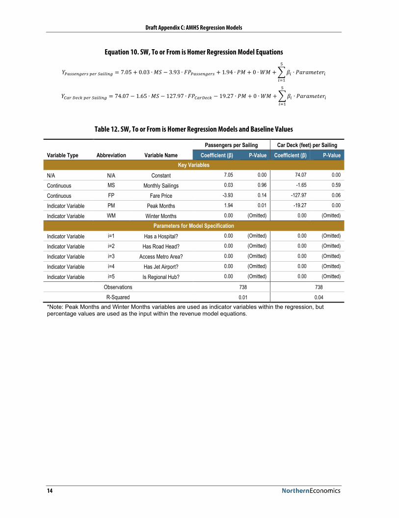
Equation 10. SW, To or From is Homer Regression Model Equations
𝑌𝑌𝑃𝑃𝑃𝑃𝑃𝑃𝑃𝑃𝑃𝑃𝑃𝑃𝑃𝑃𝑃𝑃𝑃𝑃𝑃𝑃 𝑝𝑝𝑃𝑃𝑃𝑃 𝑆𝑆𝑃𝑃𝑆𝑆𝑆𝑆𝑆𝑆𝑃𝑃𝑃𝑃 = 7.05 + 0.03 ∙ 𝑀𝑀𝑀𝑀 − 3.93 ∙ 𝐹𝐹𝐹𝐹𝑃𝑃𝑃𝑃𝑃𝑃𝑃𝑃𝑃𝑃𝑃𝑃𝑃𝑃𝑃𝑃𝑃𝑃𝑃𝑃 + 1.94 ∙ 𝐹𝐹𝑀𝑀 + 0 ∙ 𝑊𝑊𝑀𝑀 + �𝛽𝛽𝑆𝑆 ∙ 𝐹𝐹𝑃𝑃𝑃𝑃𝑃𝑃𝑃𝑃𝑃𝑃𝑃𝑃𝑃𝑃𝑃𝑃𝑆𝑆
5
𝑆𝑆=1
𝑌𝑌𝐶𝐶𝑃𝑃𝑃𝑃 𝐷𝐷𝑃𝑃𝐷𝐷𝐷𝐷 𝑝𝑝𝑃𝑃𝑃𝑃 𝑆𝑆𝑃𝑃𝑆𝑆𝑆𝑆𝑆𝑆𝑃𝑃𝑃𝑃 = 74.07− 1.65 ∙ 𝑀𝑀𝑀𝑀 − 127.97 ∙ 𝐹𝐹𝐹𝐹𝐶𝐶𝑃𝑃𝑃𝑃𝐷𝐷𝑃𝑃𝐷𝐷𝐷𝐷 − 19.27 ∙ 𝐹𝐹𝑀𝑀 + 0 ∙ 𝑊𝑊𝑀𝑀 + �𝛽𝛽𝑆𝑆 ∙ 𝐹𝐹𝑃𝑃𝑃𝑃𝑃𝑃𝑃𝑃𝑃𝑃𝑃𝑃𝑃𝑃𝑃𝑃𝑆𝑆
5
𝑆𝑆=1
Table 12. SW, To or From is Homer Regression Models and Baseline Values
Variable Type Abbreviation Variable Name Passengers per Sailing Car Deck (feet) per Sailing
Coefficient (β) P-Value Coefficient (β) P-Value Key Variables
N/A N/A Constant 7.05 0.00 74.07 0.00
Continuous MS Monthly Sailings 0.03 0.96 -1.65 0.59
Continuous FP Fare Price -3.93 0.14 -127.97 0.06
Indicator Variable PM Peak Months 1.94 0.01 -19.27 0.00
Indicator Variable WM Winter Months 0.00 (Omitted) 0.00 (Omitted)
Parameters for Model Specification
Indicator Variable i=1 Has a Hospital? 0.00 (Omitted) 0.00 (Omitted)
Indicator Variable i=2 Has Road Head? 0.00 (Omitted) 0.00 (Omitted)
Indicator Variable i=3 Access Metro Area? 0.00 (Omitted) 0.00 (Omitted)
Indicator Variable i=4 Has Jet Airport? 0.00 (Omitted) 0.00 (Omitted)
Indicator Variable i=5 Is Regional Hub? 0.00 (Omitted) 0.00 (Omitted)
Observations 738 738 R-Squared 0.01 0.04
*Note: Peak Months and Winter Months variables are used as indicator variables within the regression, but percentage values are used as the input within the revenue model equations.

Draft Appendix C: AMHS Regression Models
15
Equation 11. SW, To or From is Kodiak Regression Model Equations
𝑌𝑌𝑃𝑃𝑃𝑃𝑃𝑃𝑃𝑃𝑃𝑃𝑃𝑃𝑃𝑃𝑃𝑃𝑃𝑃𝑃𝑃 𝑝𝑝𝑃𝑃𝑃𝑃 𝑆𝑆𝑃𝑃𝑆𝑆𝑆𝑆𝑆𝑆𝑃𝑃𝑃𝑃 = 7.05 − 0.90 ∙ 𝑀𝑀𝑀𝑀 − 8.41 ∙ 𝐹𝐹𝐹𝐹𝑃𝑃𝑃𝑃𝑃𝑃𝑃𝑃𝑃𝑃𝑃𝑃𝑃𝑃𝑃𝑃𝑃𝑃𝑃𝑃 + 1.50 ∙ 𝐹𝐹𝑀𝑀 + 0 ∙ 𝑊𝑊𝑀𝑀 + �𝛽𝛽𝑆𝑆 ∙ 𝐹𝐹𝑃𝑃𝑃𝑃𝑃𝑃𝑃𝑃𝑃𝑃𝑃𝑃𝑃𝑃𝑃𝑃𝑆𝑆
5
𝑆𝑆=1
𝑌𝑌𝐶𝐶𝑃𝑃𝑃𝑃 𝐷𝐷𝑃𝑃𝐷𝐷𝐷𝐷 𝑝𝑝𝑃𝑃𝑃𝑃 𝑆𝑆𝑃𝑃𝑆𝑆𝑆𝑆𝑆𝑆𝑃𝑃𝑃𝑃 = 7.05 − 0.90 ∙ 𝑀𝑀𝑀𝑀 − 8.41 ∙ 𝐹𝐹𝐹𝐹𝐶𝐶𝑃𝑃𝑃𝑃𝐷𝐷𝑃𝑃𝐷𝐷𝐷𝐷 + 1.50 ∙ 𝐹𝐹𝑀𝑀 + 0 ∙ 𝑊𝑊𝑀𝑀 + �𝛽𝛽𝑆𝑆 ∙ 𝐹𝐹𝑃𝑃𝑃𝑃𝑃𝑃𝑃𝑃𝑃𝑃𝑃𝑃𝑃𝑃𝑃𝑃𝑆𝑆
5
𝑆𝑆=1
Table 13. SW, To or From is Kodiak Regression Models and Baseline Values
Variable Type Abbreviation Variable Name Passengers per Sailing Car Deck (feet) per Sailing
Coefficient (β) P-Value Coefficient (β) P-Value Key Variables
N/A N/A Constant 7.05 0.00 7.05 0.00
Continuous MS Monthly Sailings -0.90 0.00 -0.90 0.00
Continuous FP Fare Price -8.41 0.00 -8.41 0.00
Indicator Variable PM Peak Months 1.50 0.00 1.50 0.00
Indicator Variable WM Winter Months 0.00 (Omitted) 0.00 (Omitted)
Parameters for Model Specification
Indicator Variable i=1 Has a Hospital? 0.00 (Omitted) 0.00 (Omitted)
Indicator Variable i=2 Has Road Head? 0.00 (Omitted) 0.00 (Omitted)
Indicator Variable i=3 Access Metro Area? 0.00 (Omitted) 0.00 (Omitted)
Indicator Variable i=4 Has Jet Airport? 0.00 (Omitted) 0.00 (Omitted)
Indicator Variable i=5 Is Regional Hub? 0.00 (Omitted) 0.00 (Omitted)
Observations 746 746 R-Squared 0.05 0.02
*Note: Peak Months and Winter Months variables are used as indicator variables within the regression, but percentage values are used as the input within the revenue model equations.

Draft Appendix C: AMHS Regression Models
16
Equation 12. Metlakatla-Ketchikan and Ketchikan-Metlakatla Port-Pairs Regression Model Equations
𝑌𝑌𝑃𝑃𝑃𝑃𝑃𝑃𝑃𝑃𝑃𝑃𝑃𝑃𝑃𝑃𝑃𝑃𝑃𝑃𝑃𝑃 𝑝𝑝𝑃𝑃𝑃𝑃 𝑆𝑆𝑃𝑃𝑆𝑆𝑆𝑆𝑆𝑆𝑃𝑃𝑃𝑃 = 37.62 + 0.003 ∙ 𝑀𝑀𝑀𝑀 − 3.09 ∙ 𝐹𝐹𝐹𝐹𝑃𝑃𝑃𝑃𝑃𝑃𝑃𝑃𝑃𝑃𝑃𝑃𝑃𝑃𝑃𝑃𝑃𝑃𝑃𝑃 + 0.29 ∙ 𝐹𝐹𝑀𝑀 + 0.68 ∙ 𝑊𝑊𝑀𝑀 + �𝛽𝛽𝑆𝑆 ∙ 𝐹𝐹𝑃𝑃𝑃𝑃𝑃𝑃𝑃𝑃𝑃𝑃𝑃𝑃𝑃𝑃𝑃𝑃𝑆𝑆
5
𝑆𝑆=1
𝑌𝑌𝐶𝐶𝑃𝑃𝑃𝑃 𝐷𝐷𝑃𝑃𝐷𝐷𝐷𝐷 𝑝𝑝𝑃𝑃𝑃𝑃 𝑆𝑆𝑃𝑃𝑆𝑆𝑆𝑆𝑆𝑆𝑃𝑃𝑃𝑃 = 279.68− 0.09 ∙ 𝑀𝑀𝑀𝑀 − 39.31 ∙ 𝐹𝐹𝐹𝐹𝐶𝐶𝑃𝑃𝑃𝑃𝐷𝐷𝑃𝑃𝐷𝐷𝐷𝐷 + 3.39 ∙ 𝐹𝐹𝑀𝑀 − 0.09 ∙ 𝑊𝑊𝑀𝑀 + �𝛽𝛽𝑆𝑆 ∙ 𝐹𝐹𝑃𝑃𝑃𝑃𝑃𝑃𝑃𝑃𝑃𝑃𝑃𝑃𝑃𝑃𝑃𝑃𝑆𝑆
5
𝑆𝑆=1
Table 14. Metlakatla-Ketchikan and Ketchikan-Metlakatla Port-Pairs Regression Models and Baseline Values
Variable Type Abbreviation Variable Name Passengers per Sailing Car Deck (feet) per Sailing
Coefficient (β) P-Value Coefficient (β) P-Value Key Variables
N/A N/A Constant 37.62 0.00 279.68 0.00
Continuous MS Monthly Sailings 0.003 0.91 -0.09 0.43
Continuous FP Fare Price -3.09 0.00 -39.31 0.00
Indicator Variable PM Peak Months 0.29 0.83 3.39 0.51
Indicator Variable WM Winter Months 0.68 0.60 -0.09 0.99
Observations 66 66 R-Squared 0.33 0.55
Notes: This model is based on a separate data set from all other regression models in the study, because tickets are priced for round-trip service. Since there are only two ports within the data set, the independent variable parameters to control for available amenities are unnecessary and not included.
*Peak Months and Winter Months variables are used as indicator variables within the regression, but percentage values are used as the input within the revenue model equations.

Draft Appendix C: AMHS Regression Models
17
Equation 13. PWS for Whittier-Valdez and Valdez-Whitter Port-Pairs Regression Model Equations
𝑌𝑌𝑃𝑃𝑃𝑃𝑃𝑃𝑃𝑃𝑃𝑃𝑃𝑃𝑃𝑃𝑃𝑃𝑃𝑃𝑃𝑃 𝑝𝑝𝑃𝑃𝑃𝑃 𝑆𝑆𝑃𝑃𝑆𝑆𝑆𝑆𝑆𝑆𝑃𝑃𝑃𝑃= 24.15− 1.21 ∙ 𝑀𝑀𝑀𝑀 − 16.88 ∙ 𝐹𝐹𝐹𝐹𝑃𝑃𝑃𝑃𝑃𝑃𝑃𝑃𝑃𝑃𝑃𝑃𝑃𝑃𝑃𝑃𝑃𝑃𝑃𝑃 + 13.74 ∙ 𝐹𝐹𝐹𝐹𝐹𝐹 + 11.94 ∙ 𝑀𝑀𝑀𝑀𝑀𝑀 + 7.20 ∙ 𝑀𝑀𝐹𝐹𝑀𝑀 + 44.14∙ 𝑀𝑀𝑀𝑀𝑌𝑌 + 88.82 ∙ 𝐽𝐽𝐽𝐽𝐽𝐽 + 117.80 ∙ 𝐽𝐽𝐽𝐽𝐽𝐽 + 110.34 ∙ 𝑀𝑀𝐽𝐽𝐴𝐴 + 56.21 ∙ 𝑀𝑀𝐹𝐹𝐹𝐹 + 9.91 ∙ 𝑂𝑂𝑂𝑂𝑂𝑂 + 1.39 ∙ 𝐽𝐽𝑂𝑂𝑁𝑁
− 2.01 ∙ 𝐷𝐷𝐹𝐹𝑂𝑂 + �𝛽𝛽𝑆𝑆 ∙ 𝐹𝐹𝑃𝑃𝑃𝑃𝑃𝑃𝑃𝑃𝑃𝑃𝑃𝑃𝑃𝑃𝑃𝑃𝑆𝑆
5
𝑆𝑆=1
𝑌𝑌𝐶𝐶𝑃𝑃𝑃𝑃 𝐷𝐷𝑃𝑃𝐷𝐷𝐷𝐷 𝑝𝑝𝑃𝑃𝑃𝑃 𝑆𝑆𝑃𝑃𝑆𝑆𝑆𝑆𝑆𝑆𝑃𝑃𝑃𝑃 = 205.06 − 7.67 ∙ 𝑀𝑀𝑀𝑀 − 1027.48 ∙ 𝐹𝐹𝐹𝐹𝐶𝐶𝑃𝑃𝑃𝑃𝐷𝐷𝑃𝑃𝐷𝐷𝐷𝐷 + 32.49 ∙ 𝐹𝐹𝐹𝐹𝐹𝐹 + 41.11 ∙ 𝑀𝑀𝑀𝑀𝑀𝑀 + 56.89 ∙ 𝑀𝑀𝐹𝐹𝑀𝑀 + 266.12∙ 𝑀𝑀𝑀𝑀𝑌𝑌 + 538.19 ∙ 𝐽𝐽𝐽𝐽𝐽𝐽 + 662.59 ∙ 𝐽𝐽𝐽𝐽𝐽𝐽 + 616.64 ∙ 𝑀𝑀𝐽𝐽𝐴𝐴 + 332.75 ∙ 𝑀𝑀𝐹𝐹𝐹𝐹 + 58.84 ∙ 𝑂𝑂𝑂𝑂𝑂𝑂 + 4.34 ∙ 𝐽𝐽𝑂𝑂𝑁𝑁
− 15.09 ∙ 𝐷𝐷𝐹𝐹𝑂𝑂 + �𝛽𝛽𝑆𝑆 ∙ 𝐹𝐹𝑃𝑃𝑃𝑃𝑃𝑃𝑃𝑃𝑃𝑃𝑃𝑃𝑃𝑃𝑃𝑃𝑆𝑆
5
𝑆𝑆=1
Table 15. PWS for Whittier-Valdez and Valdez-Whitter Port-Pairs Regression Models and Baseline Values
Variable Type Abbreviation Variable Name Passengers per Sailing Car Deck (feet) per Sailing
Coefficient (β) P-Value Coefficient (β) P-Value Key Variables
N/A N/A Constant 24.15 0.00 205.06 0.00
Continuous MS Monthly Sailings -1.21 0.00 -7.67 0.00
Continuous FP Fare Price -16.88 0.00 -1027.48 0.05
Indicator Variable FEB February 13.74 0.00 32.49 0.20
Indicator Variable MAR March 11.94 0.00 41.11 0.09
Indicator Variable APR April 7.20 0.08 56.89 0.02
Indicator Variable MAY May 44.14 0.00 266.12 0.00
Indicator Variable JUN June 88.82 0.00 538.19 0.00
Indicator Variable JUL July 117.80 0.00 662.59 0.00
Indicator Variable AUG August 110.34 0.00 616.64 0.00
Indicator Variable SEP September 56.21 0.00 332.75 0.00
Indicator Variable OCT October 9.91 0.02 58.84 0.02
Indicator Variable NOV November 1.39 0.75 4.34 0.87
Indicator Variable DEC December -2.01 0.66 -15.09 0.57
Parameters for Model Specification Indicator Variable i=1 Has a Hospital? 0.00 (Omitted) 0.00 (Omitted)
Indicator Variable i=2 Has Road Head? 0.00 (Omitted) 0.00 (Omitted)
Indicator Variable i=3 Is Metro Area? 0.00 (Omitted) 0.00 (Omitted)
Indicator Variable i=4 Has Jet Airport? 0.00 (Omitted) 0.00 (Omitted)
Indicator Variable i=5 Is Regional Hub? 0.00 (Omitted) 0.00 (Omitted)
Observations 226 226 R-Squared 0.87 0.88

Draft Appendix C: AMHS Regression Models
18
Equation 14. Lynn Canal for Haines-Skagway and Skagway-Haines Port-Pairs Regression Model Equations
𝑌𝑌𝑃𝑃𝑃𝑃𝑃𝑃𝑃𝑃𝑃𝑃𝑃𝑃𝑃𝑃𝑃𝑃𝑃𝑃𝑃𝑃 𝑝𝑝𝑃𝑃𝑃𝑃 𝑆𝑆𝑃𝑃𝑆𝑆𝑆𝑆𝑆𝑆𝑃𝑃𝑃𝑃= 20.63− 0.64 ∙ 𝑀𝑀𝑀𝑀 − 2.81 ∙ 𝐹𝐹𝐹𝐹𝑃𝑃𝑃𝑃𝑃𝑃𝑃𝑃𝑃𝑃𝑃𝑃𝑃𝑃𝑃𝑃𝑃𝑃𝑃𝑃 + 1.41 ∙ 𝐹𝐹𝐹𝐹𝐹𝐹 + 3.44 ∙ 𝑀𝑀𝑀𝑀𝑀𝑀 + 9.81 ∙ 𝑀𝑀𝐹𝐹𝑀𝑀 + 24.65 ∙ 𝑀𝑀𝑀𝑀𝑌𝑌+ 45.12 ∙ 𝐽𝐽𝐽𝐽𝐽𝐽 + 61.37 ∙ 𝐽𝐽𝐽𝐽𝐽𝐽 + 56.14 ∙ 𝑀𝑀𝐽𝐽𝐴𝐴 + 34.61 ∙ 𝑀𝑀𝐹𝐹𝐹𝐹 + 12.27 ∙ 𝑂𝑂𝑂𝑂𝑂𝑂 + 4.43 ∙ 𝐽𝐽𝑂𝑂𝑁𝑁 + 0.45 ∙ 𝐷𝐷𝐹𝐹𝑂𝑂
+ �𝛽𝛽𝑆𝑆 ∙ 𝐹𝐹𝑃𝑃𝑃𝑃𝑃𝑃𝑃𝑃𝑃𝑃𝑃𝑃𝑃𝑃𝑃𝑃𝑆𝑆
5
𝑆𝑆=1
𝑌𝑌𝐶𝐶𝑃𝑃𝑃𝑃 𝐷𝐷𝑃𝑃𝐷𝐷𝐷𝐷 𝑝𝑝𝑃𝑃𝑃𝑃 𝑆𝑆𝑃𝑃𝑆𝑆𝑆𝑆𝑆𝑆𝑃𝑃𝑃𝑃 = 165.95− 5.95 ∙ 𝑀𝑀𝑀𝑀 − 121.92 ∙ 𝐹𝐹𝐹𝐹𝐶𝐶𝑃𝑃𝑃𝑃𝐷𝐷𝑃𝑃𝐷𝐷𝐷𝐷 + 1.45 ∙ 𝐹𝐹𝐹𝐹𝐹𝐹 + 32.10 ∙ 𝑀𝑀𝑀𝑀𝑀𝑀 + 105.89 ∙ 𝑀𝑀𝐹𝐹𝑀𝑀 + 230.11∙ 𝑀𝑀𝑀𝑀𝑌𝑌 + 429.27 ∙ 𝐽𝐽𝐽𝐽𝐽𝐽 + 557.05 ∙ 𝐽𝐽𝐽𝐽𝐽𝐽 + 516.70 ∙ 𝑀𝑀𝐽𝐽𝐴𝐴 + 308.27 ∙ 𝑀𝑀𝐹𝐹𝐹𝐹 + 113.15 ∙ 𝑂𝑂𝑂𝑂𝑂𝑂 + 35.29
∙ 𝐽𝐽𝑂𝑂𝑁𝑁 + 3.47 ∙ 𝐷𝐷𝐹𝐹𝑂𝑂 + �𝛽𝛽𝑆𝑆 ∙ 𝐹𝐹𝑃𝑃𝑃𝑃𝑃𝑃𝑃𝑃𝑃𝑃𝑃𝑃𝑃𝑃𝑃𝑃𝑆𝑆
5
𝑆𝑆=1
Table 16. Lynn Canal for Haines-Skagway and Skagway-Haines Port-Pairs Regression Models and Baseline Values
Variable Type Abbreviation Variable Name Passengers per Sailing Car Deck (feet) per Sailing
Coefficient (β) P-Value Coefficient (β) P-Value Key Variables
N/A N/A Constant 20.63 0.00 165.95 0.00
Continuous MS Monthly Sailings -0.64 0.00 -5.96 0.00
Continuous FP Fare Price -2.81 0.00 -121.92 0.28
Indicator Variable FEB February 1.41 0.40 1.45 0.94
Indicator Variable MAR March 3.44 0.04 32.10 0.08
Indicator Variable APR April 9.81 0.00 105.89 0.00
Indicator Variable MAY May 24.65 0.00 230.11 0.00
Indicator Variable JUN June 45.12 0.00 429.27 0.00
Indicator Variable JUL July 61.37 0.00 557.05 0.00
Indicator Variable AUG August 56.14 0.00 516.70 0.00
Indicator Variable SEP September 34.61 0.00 308.27 0.00
Indicator Variable OCT October 12.27 0.00 113.15 0.00
Indicator Variable NOV November 4.43 0.01 35.29 0.05
Indicator Variable DEC December 0.45 0.79 3.47 0.85
Parameters for Model Specification Indicator Variable i=1 Has a Hospital? 0.00 (Omitted) 0.00 (Omitted)
Indicator Variable i=2 Has Road Head? 0.00 (Omitted) 0.00 (Omitted)
Indicator Variable i=3 Is Metro Area? 0.00 (Omitted) 0.00 (Omitted)
Indicator Variable i=4 Has Jet Airport? 0.00 (Omitted) 0.00 (Omitted)
Indicator Variable i=5 Is Regional Hub? 0.00 (Omitted) 0.00 (Omitted)
Observations 252 252 R-Squared 0.91 0.88

Draft Appendix C: AMHS Regression Models
19
Equation 15. Cross Gulf for Service to Chenega Bay, Ouzinkie, Port Lions, and Seldovia Equations
𝑌𝑌𝑃𝑃𝑃𝑃𝑃𝑃𝑃𝑃𝑃𝑃𝑃𝑃𝑃𝑃𝑃𝑃𝑃𝑃𝑃𝑃 𝑝𝑝𝑃𝑃𝑃𝑃 𝑆𝑆𝑃𝑃𝑆𝑆𝑆𝑆𝑆𝑆𝑃𝑃𝑃𝑃 = 73.99 + 0.57 ∙ 𝑀𝑀𝑀𝑀 − 38.40 ∙ 𝐹𝐹𝐹𝐹𝑃𝑃𝑃𝑃𝑃𝑃𝑃𝑃𝑃𝑃𝑃𝑃𝑃𝑃𝑃𝑃𝑃𝑃𝑃𝑃 + 4.74 ∙ 𝐹𝐹𝑀𝑀 − 5.29 ∙ 𝑊𝑊𝑀𝑀 + �𝛽𝛽𝑆𝑆 ∙ 𝐹𝐹𝑃𝑃𝑃𝑃𝑃𝑃𝑃𝑃𝑃𝑃𝑃𝑃𝑃𝑃𝑃𝑃𝑆𝑆
5
𝑆𝑆=1
𝑌𝑌𝐶𝐶𝑃𝑃𝑃𝑃 𝐷𝐷𝑃𝑃𝐷𝐷𝐷𝐷 𝑝𝑝𝑃𝑃𝑃𝑃 𝑆𝑆𝑃𝑃𝑆𝑆𝑆𝑆𝑆𝑆𝑃𝑃𝑃𝑃 = 432.03 + 26.87 ∙ 𝑀𝑀𝑀𝑀 − 942.54 ∙ 𝐹𝐹𝐹𝐹𝐶𝐶𝑃𝑃𝑃𝑃𝐷𝐷𝑃𝑃𝐷𝐷𝐷𝐷 − 14.10 ∙ 𝐹𝐹𝑀𝑀 + 17.35 ∙ 𝑊𝑊𝑀𝑀 + �𝛽𝛽𝑆𝑆 ∙ 𝐹𝐹𝑃𝑃𝑃𝑃𝑃𝑃𝑃𝑃𝑃𝑃𝑃𝑃𝑃𝑃𝑃𝑃𝑆𝑆
5
𝑆𝑆=1
Table 17. Cross Gulf for Service to Chenega Bay, Ouzinkie, Port Lions, and Seldovia Regression Models and Baseline Values
Variable Type Abbreviation Variable Name Passengers per Sailing Car Deck (feet) per Sailing
Coefficient (β) P-Value Coefficient (β) P-Value Key Variables
N/A N/A Constant 73.99 0.00 432.03 0.00
Continuous MS Monthly Sailings 0.57 0.46 26.87 0.00
Continuous FP Fare Price -38.40 0.00 -942.54 0.00
Indicator Variable PM Peak Months 4.74 0.00 -14.10 0.11
Indicator Variable WM Winter Months -5.29 0.00 17.35 0.27
Parameters for Model Specification
Indicator Variable i=1 Has a Hospital? 9.87 0.00 107.59 0.00
Indicator Variable i=2 Has Road Head? 0.88 0.87 47.05 0.45
Indicator Variable i=3 Access Metro Area? 7.62 0.16 52.54 0.40
Indicator Variable i=4 Has Jet Airport? -58.48 0.00 -429.51 0.00
Indicator Variable i=5 Is Regional Hub? -10.40 0.17 -54.62 0.53
Observations 1,209 1,209 R-Squared 0.63 0.44
*Note: Peak Months and Winter Months variables are used as indicator variables within the regression, but percentage values are used as the input within the revenue model equations.

Draft Appendix C: AMHS Regression Models
20
Equation 16. Cross Gulf for Service to Chenega Bay, Ouzinkie, Port Lions, and Seldovia, When To or From is Not Bellingham Equations
𝑌𝑌𝑃𝑃𝑃𝑃𝑃𝑃𝑃𝑃𝑃𝑃𝑃𝑃𝑃𝑃𝑃𝑃𝑃𝑃𝑃𝑃 𝑝𝑝𝑃𝑃𝑃𝑃 𝑆𝑆𝑃𝑃𝑆𝑆𝑆𝑆𝑆𝑆𝑃𝑃𝑃𝑃 = 14.23 + 0.28 ∙ 𝑀𝑀𝑀𝑀 − 39.02 ∙ 𝐹𝐹𝐹𝐹𝑃𝑃𝑃𝑃𝑃𝑃𝑃𝑃𝑃𝑃𝑃𝑃𝑃𝑃𝑃𝑃𝑃𝑃𝑃𝑃 + 3.44 ∙ 𝐹𝐹𝑀𝑀 − 3.80 ∙ 𝑊𝑊𝑀𝑀 + �𝛽𝛽𝑆𝑆 ∙ 𝐹𝐹𝑃𝑃𝑃𝑃𝑃𝑃𝑃𝑃𝑃𝑃𝑃𝑃𝑃𝑃𝑃𝑃𝑆𝑆
5
𝑆𝑆=1
𝑌𝑌𝐶𝐶𝑃𝑃𝑃𝑃 𝐷𝐷𝑃𝑃𝐷𝐷𝐷𝐷 𝑝𝑝𝑃𝑃𝑃𝑃 𝑆𝑆𝑃𝑃𝑆𝑆𝑆𝑆𝑆𝑆𝑃𝑃𝑃𝑃 = −50.39 + 28.09 ∙ 𝑀𝑀𝑀𝑀 − 952.85 ∙ 𝐹𝐹𝐹𝐹𝐶𝐶𝑃𝑃𝑃𝑃𝐷𝐷𝑃𝑃𝐷𝐷𝐷𝐷 − 18.15 ∙ 𝐹𝐹𝑀𝑀 + 28.64 ∙ 𝑊𝑊𝑀𝑀 + �𝛽𝛽𝑆𝑆 ∙ 𝐹𝐹𝑃𝑃𝑃𝑃𝑃𝑃𝑃𝑃𝑃𝑃𝑃𝑃𝑃𝑃𝑃𝑃𝑆𝑆
5
𝑆𝑆=1
Table 18. Cross Gulf for Service to Chenega Bay, Ouzinkie, Port Lions, and Seldovia, When To or From is Not Bellingham Regression Models and Baseline Values
Variable Type Abbreviation Variable Name Passengers per Sailing Car Deck (feet) per Sailing
Coefficient (β) P-Value Coefficient (β) P-Value Key Variables
N/A N/A Constant 14.23 0.12 -50.39 0.68
Continuous MS Monthly Sailings 0.28 0.71 28.09 0.01
Continuous FP Fare Price -39.02 0.00 -952.85 0.00
Indicator Variable PM Peak Months 3.44 0.00 -18.15 0.07
Indicator Variable WM Winter Months -3.80 0.01 28.64 0.10
Parameters for Model Specification
Indicator Variable i=1 Has a Hospital? 11.15 0.00 140.99 0.00
Indicator Variable i=2 Has Road Head? 0.17 0.97 44.62 0.47
Indicator Variable i=3 Access Metro Area? 10.21 0.03 92.88 0.13
Indicator Variable i=4 Has Jet Airport? 0.59 0.93 34.51 0.68
Indicator Variable i=5 Is Regional Hub? -9.66 0.13 -70.34 0.41
Observations 936 936 R-Squared 0.29 0.22
*Note: Peak Months and Winter Months variables are used as indicator variables within the regression, but percentage values are used as the input within the revenue model equations.


![AFI AMHS Manual - icao.int€¦ · AFI AMHS Manual [9] Version 1.0 21/07/2011 1 Structure of the AFI AMHS Manual 1.1 The AFI AMHS Manual consists of the “Main Part” and the Appendices](https://img.dokumen.tips/doc/110x75/5f1097617e708231d449dca7/afi-amhs-manual-icaoint-afi-amhs-manual-9-version-10-21072011-1-structure.jpg)