Domination number of cubic graphs with large girth

Domination Number ofCubic Graphs WithLarge Girth

Daniel Kral’,1 Petr Skoda,2 and Jan Volec3

1DEPARTMENT OF APPLIED MATHEMATICS AND INSTITUTEFOR THEORETICAL COMPUTER SCIENCE

FACULTY OF MATHEMATICS AND PHYSICSCHARLES UNIVERSITY, MALOSTRANSKE

NAMESTI 25, 118 00 PRAGUE, CZECH REPUBLICE-mail: [email protected]

2DEPARTMENT OF MATHEMATICSSIMON FRASER UNIVERSITY, 8888 UNIVERSITY DRIVE BURNABY

BC V5A 1S6, CANADAE-mail: [email protected]

3DEPARTMENT OF APPLIED MATHEMATICSFACULTY OF MATHEMATICS AND PHYSICS

CHARLES UNIVERSITY, MALOSTRANSKENAMESTI 25, 118 00 PRAGUE, CZECH REPUBLIC

E-mail: [email protected]

Received September 5, 2009; Revised September 30, 2010

Published online 1 February 2011 in Wiley Online Library (wileyonlinelibrary.com).DOI 10.1002/jgt.20568

Abstract: We show that every n-vertex cubic graph with girth at leastg have domination number at most 0.299871n+O(n /g)<3n /10+O(n /g)

This research was done when the Petr Skoda was a student of Department ofApplied Mathematics, Faculty of Mathematics and Physics, Charles University.

Contract grant sponsor: Czech-Slovenian Bilateral Project; Contract grant numbers:project MEB 090805; BI-CZ/08-09-005 (to D. K., P. S., and J. V.); Contract grantsponsor: Czech Ministry of Education; Contract grant number: project 1M0545(to D. K.); Contract grant sponsor: GACR; Contract grant number: 201/09/0197(to D. K.).Journal of Graph Theory� 2011 Wiley Periodicals, Inc.

131

132 JOURNAL OF GRAPH THEORY

which improves a previous bound of 0.321216n+O(n /g) by Rautenbachand Reed. � 2011 Wiley Periodicals, Inc. J Graph Theory 69: 131–142, 2012

Keywords: domination; dominating number; cubic graphs; probabilistic method

1. INTRODUCTION

The notion of a dominating set is a classical notion in graph theory with a large amountof literature associated with it. For the sake of completeness, let us recall that a setD of vertices of a graph G is dominating if every vertex of G is contained in D orhas a neighbor in D and the domination number �(G) of G is the smallest size of adominating set of G. In this article, we study the domination number of cubic graphs,i.e., graphs where every vertex has degree three.

In 1996, Reed [9] conjectured that every n-vertex connected cubic graph has domi-nation number at most �n /3�. Though the conjecture turned out to be false [4, 3], theconjecture becomes true with the additional assumption that the cubic graph has girthat least g, i.e., it has no cycles of length less than g. The first results in this direc-tion are the bounds on the domination number of ( 1

3 +1/ (3g+3))n of Kawarabayashiet al. [2] for bridgeless n-vertex cubic graphs with girth at least g for g divisibleby three and ( 1

3 +8/ (3g2))n of Kostochka and Stodolsky [5] for all n-vertex cubicgraphs with girth at least g. The magic threshold of n /3 was first beaten for cubicgraphs with large girth by Lowenstein and Rautenbach [6] who showed that everyn-vertex cubic graph with girth at least g≥5 contains a dominating set of size at most( 44

135 + 82135g )n≈0.325926n+O(n /g). The bound was further improved by Rautenbach

and Reed [8] to 0.321216n+O(n /g).We further improve these bounds and manage to lower them below the 3n /10

threshold. Our main result is the following:

Theorem 1. Let G be an n-vertex cubic graph with girth at least g. The dominationnumber of G is at most 0.299871n+O(n /g)≤3n /10+O(n /g).

At this point, we remark that numerical computations involved in our argumentwere done using a computer (but the rules given in Fig. 3 were generated byhand) though the whole proof can be easily verified to be correct without computerassistance.

Before we start the exposition of our proof, let us mention a connection to randomcubic graphs. It is known that the domination number of a random cubic graph isalmost surely at least 0.2636n [7] and at most 0.2794n [1]. A random cubic graphalmost surely contains only a bounded number of cycles of length less than g for everyfixed integer g and thus the lower bounds on the domination number of random cubicgraphs are also lower bounds for cubic graphs with large girth; conversely, Wormald[10] has recently developed a technique for translating upper bounds (obtained in aspecific but quite general way) for the independence number of random cubic graphsto cubic graphs with large girth and his method could be applied to other parameters.Hence, the known bounds for the domination number of random cubic graphs indicatehow tight our result can be.

Journal of Graph Theory DOI 10.1002/jgt

DOMINATION NUMBER OF CUBIC GRAPHS 133

2. PROOF

Our proof is based on enhancing the probabilistic argument from [8] in two ways:auxiliary paths covering a given graph are randomly distributed into several levels(as opposed to two levels used in [8]) and a more sophisticated algorithm is usedto construct the dominating set. The analysis that we present reflects these twodevelopments.

In this section, we first provide a general overview of our method and illustrateit on a small example. At the end, we then apply the method in a setting yieldingTheorem 1.

A. Overview

In this subsection, we explain main ideas of our method and we later provide necessarytechnical details related to it. Fix a cubic bridgeless graph G with girth at least g andalso fix an integer K which determines the number of levels as defined later. Considera 2-factor of G (which exists by the Petersen theorem) and decompose each cycle ofthe 2-factor into vertex-disjoint paths P1, . . . ,P� with the number of vertices betweeng /4K and g /2K (this is possible since the length of each cycle of the 2-factor is atleast g). The vertices of the paths P1, . . . ,P� are considered to be ordered from one endof the path toward the other; a mate of a vertex v is the neighbor of G not adjacent tov on the cycle of the 2-factor.

A dominating set D of G will be given by a labeling of vertices of G we construct.Each vertex of G will be assigned an input label which is one of the symbols +, ×, •and ◦, and an output label which is one of the symbols ⊕, ⊗ and . The dominatingset D will contain the vertices with input label + or output label ⊗ (as well as severalothers, see the next subsection for an exhaustive definition). We explain the intuitivemeaning of the labels later.

Split the paths P1, . . . ,Pk into K sets P1, . . . ,PK including each path to a singleset randomly uniformly and independently of the other paths. The sets P1, . . . ,PK arereferred to as levels and vertices on paths in Pi are said to be on the level i. First, thevertices contained in paths of P1 are assigned labels, then those in paths of P2, etc. LetP be a path included in Pi and assume that the vertices of the paths in P1 ∪·· ·∪Pi−1have already been labeled. The input label of a vertex of P is:

• the symbol + if its mate is on a path in P1 ∪·· ·∪Pi−1 and its output label is ⊕,• the symbol × if its mate is on a path in P1 ∪·· ·∪Pi−1 and its output label is ⊗,• the symbol • if its mate is on a path in P1 ∪·· ·∪Pi−1 and its output label is ,• the symbol • if its mate is on a path in Pi, and• the symbol ◦ if its mate is on a path in Pi+1 ∪·· ·∪Pk.

The output labels are assigned in blocks using rules. Each rule is a pair of a sequenceof input symbols and the symbol ? which represents a wild-card and a sequence ofoutput symbols. The lengths of the two sequences will always be the same. We usuallywrite an arrow between the two sequences, e.g., one of the rules can be +?→.Naturally, the sequence of input symbols and ? is called the left-hand side of the ruleand the sequence of output symbols the right-hand side. Finally, if �→� is a rule, weuse �i as the ith symbol of � and �i as the ith symbol of �. An example of a set ofrules is given in Figure 1.



FIGURE 1. An example of a (correct) set of rules.

We look for a rule whose left-hand side matches the input labels of vertices at thebeginning of P. All the considered rule sets will have the property that such a ruleis unique. The right-hand side of the rule then determines the output labels. We thenmove after the vertices with output labels assigned and again look for a rule whoseleft-hand side matches the input labels of vertices without output labels. After findinga suitable rule, the next group of vertices is assigned output labels, we move after themand continue in this way until we reach the end of the path P. Note that it can happenthat we are left with few vertices without output labels at the end of the path P—thiswill be handled in the next subsection.

The meaning of output labels is the following: if a vertex v is labelled with ⊗, thenv should be included to the dominating set D. If a vertex v is labelled with ⊕, then itsmate should be included to D (this output label can only be assigned to vertices withinput labels ◦, i.e., with mates on higher levels). Finally, if v is labelled with , thenit is dominated by one of its neighbors on its path or by its mate on a lower level.The input labels can be interpreted as follows: the label + represents that v is includedto D, the label × represents that its mate on a lower label is included, the label •represents that neither v nor its mate has yet not been included to D and the mate ison a lower or the same level, and the label ◦ represents that a mate is on a higherlevel.

A set of rules is called correct if for every rule �→� the following holds:

• if �i is • or ◦ and neither �i−1 nor �i+1 (if they exist) is +, then �i is ⊕ or oneof the symbols �i−1, �i, and �i+1 is ⊗, and

• if �i is ⊕, then �i is ◦.

Intuitively, if a set of rules is correct, then the set D containing the vertices with inputlabel + or output label ⊗ is always dominating and the label ⊕ can be only assignedto vertices with mates on higher levels. The set of rules given in Figure 1 is correct.

B. Analysis and Adjustments

In this subsection, we provide further details on the labeling procedure and analyze it.The first thing to cope with is the fact that a cubic graph need not have a 2-factor. Thisis handled in a way analogous to that used in [8]. For a collection of vertex-disjointpaths, a vertex is covered if it is contained in one of the paths.

Lemma 1. For every K ≥2, g and n-vertex cubic graph G with girth at least g, thereexists a collection of at most (3+8K) / (2g)n vertex disjoint paths in G with the numberof vertices less than g /2K that covers at least n−O(n /g) vertices of G. Moreover, allvertices on the paths can be grouped into pairs of vertices adjacent through an edgenot contained in the paths.



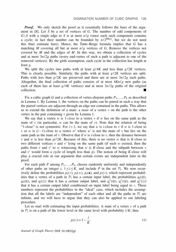
Proof. We only sketch the proof as it essentially follows the lines of the argu-ment in [8]. Let S be a set of vertices of G. The number of odd components ofG\S with a single edge to S is at most n /g (since each such component containsa cycle; in fact their number can be bounded by n /2�(g), but we do not needthis finer estimate here). Hence, the Tutte–Berge formula implies that G has amatching M covering all but at most n /g vertices of G. Remove the vertices notcovered by M and the edges of M. In this way, we obtain a collection of cyclesand at most 3n /2g paths (every end-vertex of such a path is adjacent to one of theremoved vertices). By the girth assumption, each cycle in the collection has length atleast g.

We split the cycles into paths with at least g /4K and less than g /2K vertices.This is clearly possible. Similarly, the paths with at least g /2K vertices are split.Paths with less than g /2K are preserved and there are at most 3n /2g such paths.Altogether, the final collection of paths consists of at most 4Kn /g new paths (aseach of them has at least g /4K vertices) and at most 3n /2g paths of the originalcollection. �

Fix a cubic graph G and a collection of vertex-disjoint paths P1, . . . ,Pk as describedin Lemma 1. By Lemma 1, the vertices on the paths can be paired in such a way thatthe paired vertices are adjacent through an edge not contained in the paths. This allowsus to extend the definition of a mate: a mate of a vertex v on the path is the othervertex in the pair containing v given by Lemma 1.

We say that a vertex w is 1-close to a vertex v if w lies on the same path as themate of v (in particular, w can be the mate of v). Note that the relation of being“1-close” is not symmetric. For i>1, we say that w is i-close to v if w is 1-close tov or w is (i−1)-close to a vertex w′ where w′ is not the mate of v but lies on thesame path as the mate of v. Observe that if w is i-close to v, then the distance betweenv and w is less than gi /2K. Because of this, there is no vertex w that is K-close totwo different vertices v and v′ lying on the same path (if such w existed, then thepaths from v and v′ to w witnessing that w is K-close and the subpath between vand v′ would form a cycle of length less than g). The notion of being K-close willplay a crucial role in our argument that certain events are independent later in theproof.

For each path P among P1, . . . ,Pk, choose randomly uniformly and independentlyof other paths an integer i, 1≤ i≤K, and include P in the set Pi. We now recur-sively define the probabilities pi(+), pi(×), pi(•), and pi(◦), which represent probabil-ities that a vertex of a path in Pi has a certain input label, the probabilities qi(⊕),qi(⊗), and qi() that it has a certain output label, and q◦

i (⊕), q◦i (⊗), and q◦

i ()that it has a certain output label conditioned on input label being equal to ◦. Thesenumbers represent the probabilities in the “ideal” case, which includes the assump-tion that all the labels are “independent” of each other and all the paths in Pi areinfinite, and we will have to argue that they can also be applied to our labelingprocedure.

Let us start with estimating the input probabilities. A mate of a vertex v of a pathin Pi is on a path of the lower level or the same level with probability i /K; thus

pi(◦)=1− i

K. (1)



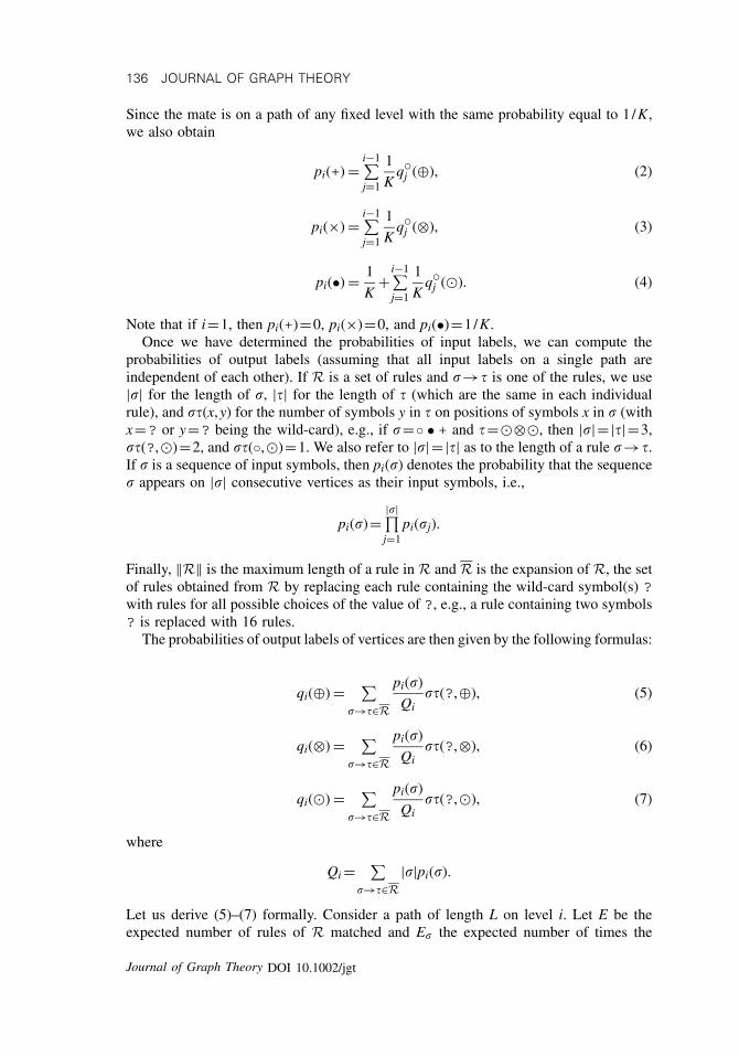
Since the mate is on a path of any fixed level with the same probability equal to 1 /K,we also obtain

pi(+) =i−1∑j=1

1

Kq◦

j (⊕), (2)

pi(×) =i−1∑j=1

1

Kq◦

j (⊗), (3)

pi(•) = 1

K+

i−1∑j=1

1

Kq◦

j (). (4)

Note that if i=1, then pi(+)=0, pi(×)=0, and pi(•)=1/K.Once we have determined the probabilities of input labels, we can compute the

probabilities of output labels (assuming that all input labels on a single path areindependent of each other). If R is a set of rules and �→� is one of the rules, we use|�| for the length of �, |�| for the length of � (which are the same in each individualrule), and ��(x,y) for the number of symbols y in � on positions of symbols x in � (withx=? or y=? being the wild-card), e.g., if �=◦ • + and �=⊗, then |�|=|�|=3,��(?,)=2, and ��(◦,)=1. We also refer to |�|=|�| as to the length of a rule �→�.If � is a sequence of input symbols, then pi(�) denotes the probability that the sequence� appears on |�| consecutive vertices as their input symbols, i.e.,

pi(�)=|�|∏j=1

pi(�j).

Finally, ‖R‖ is the maximum length of a rule in R and R is the expansion of R, the setof rules obtained from R by replacing each rule containing the wild-card symbol(s) ?with rules for all possible choices of the value of ?, e.g., a rule containing two symbols? is replaced with 16 rules.

The probabilities of output labels of vertices are then given by the following formulas:

qi(⊕) = ∑�→�∈R

pi(�)

Qi��(?,⊕), (5)

qi(⊗) = ∑�→�∈R

pi(�)

Qi��(?,⊗), (6)

qi() = ∑�→�∈R

pi(�)

Qi��(?,), (7)

where

Qi =∑

�→�∈R|�|pi(�).

Let us derive (5)–(7) formally. Consider a path of length L on level i. Let E be theexpected number of rules of R matched and E� the expected number of times the



rule �→� is matched. In the analysis that follows, it is convenient to think of theconsidered path as a sufficiently long part of an infinite path which is consistent withour arguments presented later. When we start matching, the probability that the rule�→� is matched is equal to pi(�). Hence, the expected number of times E� the rule�→� is matched is pi(�)E. By the linearity of expectations, we also have that

∑�→�∈R

E�|�|=L.

By the definition of Qi, we obtain that E=L /Qi and E� =Lpi(�) /Qi. Summing overall rules �→�∈R, we obtain the expected numbers of output labels of the vertices ofa path, e.g., the expected number of the output label ⊕ is

∑�→�∈R

Lpi(�)

Qi��(?,⊕).

The obtained quantities after dividing by L represent the corresponding probabilitiesas given in (5)–(7).

Similarly, the probabilities conditioned on the appearance of the input symbol ◦ aregiven by

q◦i (⊕) = ∑

�→�∈R

pi(�)

Q◦i

��(◦,⊕), (8)

q◦i (⊗) = ∑

�→�∈R

pi(�)

Q◦i

��(◦,⊗), (9)

q◦i () = ∑

�→�∈R

pi(�)

Q◦i

��(◦,), (10)

where

Q◦i = ∑

�→�∈R��(◦,?)pi(�).

The just-defined quantities for the set of rules given in Figure 1 and K =5 are givenin Figure 2.

FIGURE 2. The probabilities given by (1)–(10) for the set of rulesfrom Figure 1 and K =5.



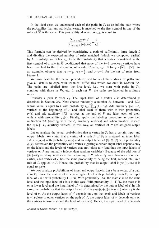
In the ideal case, we understand each of the paths in Pi as an infinite path wherethe probability that any particular vertex is matched to the first symbol in one of therules of R is the same. This probability, denoted as ri,1, is equal to

∑�→�∈R pi(�)∑

�→�∈R |�|pi(�)= 1

Qi.

This formula can be derived by considering a path of sufficiently large length Land dividing the expected number of rules matched (which we computed earlier)by L. Similarly, we define ri,j to be the probability that a vertex is matched to thefirst symbol of a rule in R conditioned that none of the j−1 previous vertices havebeen matched to the first symbol of a rule. Clearly, ri,j =0 for j>‖R‖=‖R‖. Asan example, observe that r1,1 = 1

3 , r1,2 = 12 , and r1,3 =1 for the set of rules from

Figure 1.We now describe the actual procedure used to label the vertices of paths and

give all details to cope with technical difficulties which we omit in Section 2A.The paths are labelled from the first level, i.e., we start with paths in P1,continue with those in P2, etc. In each set Pi, the paths are labelled in arbitraryorder.

Consider a path P from Pi. The input label of a vertex v is determined asdescribed in Section 2A. Next choose randomly a number �0 between 1 and ‖R‖whose value is equal to � with probability ri,�

∏�−1j=1 (1−ri,j). Add auxiliary ‖R‖−�0

vertices at the beginning of P and label each of them with x with probabilitypi(x) and add auxiliary ‖R‖ vertices at the end of P and label each of themwith x with probability pi(x). Finally, apply the labeling procedure as describedin Section 2A (starting with the �0 auxiliary vertices) and when finished, discardthe 2‖R‖−�0 auxiliary vertices. In this way, all vertices of P are assigned outputlabels.

Let us analyze the actual probabilities that a vertex in Pi has a certain input andoutput labels. We claim that a vertex of a path P of Pi is assigned an input labelx∈{+,×,•,◦} with probability pi(x) and an output label x∈{⊕,⊗,} with probabilityqi(x). Moreover, the probability of a vertex v getting a certain input label depends onlyon the labels and the levels of vertices that are i-close to v (and thus the input labels ofvertices on P are mutually independent random variables). Because of the addition of‖R‖−�0 auxiliary vertices at the beginning of P, where �0 was chosen as describedearlier, each vertex of P has the same probability of being the first, second, etc., in arule of R applied to P. Hence, the probability that its output label is y∈{⊕,⊗,} isequal to qi(y).

We now analyze probabilities of input and output labels. Let v be a vertex of a pathP in Pi. Since the mate v′ of v is on a higher level with probability 1− i /K, the inputlabel of v is ◦ with probability 1− i /K. With probability 1 /K, the mate v′ is on the samelevel and the input label of v is • in this case. With probability (i−1) /K, the mate v′ ison a lower level and the input label of v is determined by the output label of v′ in thiscase; the probability that the output label of v′ is y∈{⊕,⊗,} is q◦

j (y) where j is thelevel of v′. As the output label of v′ depends only on the levels and labels of vertices(i−1)-close to other vertices on the path of v′, the output label of v′ depends only onthe vertices i-close to v (and the level of its mate). Hence, the input label of v depends



only on the labels and the levels of vertices i-close to v. In particular, input labels ofall the vertices of P are mutually independent. Since the probability of v being thefirst, second, etc. in a particular rule of R applied to it is the same because of paddingwith �0 auxiliary vertices, the probability that the output label of v is y∈{⊕,⊗,} isequal to qi(y) and the probability that the output label is y conditioned by its inputlabel being ◦ is q◦

i (y).Consider a labeling of the vertices of G constructed in the just described way. The

dominating set D for a graph G is formed by the following vertices:

• vertices not covered by the paths in P1 ∪·· ·∪Pk,• vertices with input label +,• vertices with output label ⊗, and• the first and the last vertex of each path in P1 ∪·· ·∪Pk.

Let us verify that D is a dominating set: a vertex v not covered by the paths inP1 ∪·· ·∪Pk is in D. Vertices on paths P1 ∪·· ·∪Pk with input label different from + andoutput label different from ⊗ are dominated either by their mates or by their neighborson paths with auxiliary vertices (assuming the set of rules is correct). However, sincethe auxiliary vertices were discarded, the first and the last vertex of each path may notbe dominated in this way—this has been repaired by adding them to D (regardless oftheir labels).

It remains to estimate the expected size of D. The expected size of D is equal tothe sum of the expected number of vertices with output label ⊗ or ⊕ (note that eachvertex with input label + has a mate with output label ⊕), the number of vertices notcovered by paths (which is at most O(n /g)) and twice the number of paths becauseof the inclusion of their first and last vertices to D (this number is also O(n /g)). Theprobability that a vertex v has output label ⊕ is q1(⊕)+·· ·+qK(⊕) /K as the pathcontaining v is included to any of the K levels with the same probability. Similarly, itsoutput label is ⊗ with probability (q1(⊗)+·· ·+qK(⊗)) /K.

We summarize the results presented in this section in the following lemma:

Lemma 2. Let R be a correct set of rules, K ≥2 an integer, and qi(⊕) and qi(⊗)quantities determined using (1)–(10). If the procedure described in this subsectiongiven by the set of rules R and the integer K is applied to any cubic n-vertexgraph with girth at least g, then it produces a dominating set with expected sizeequal to

∑Ki=1(qi(⊕)+qi(⊗))

Kn+O

(n

g

).

Note that already the simple set of rules given in Figure 1 for K =5 yields byLemma 2 that the domination number of a cubic graph with girth at least g is at most0.313972n+O(n /g), an improvement on the bound of Rautenbach and Reed from [8].

C. Finale

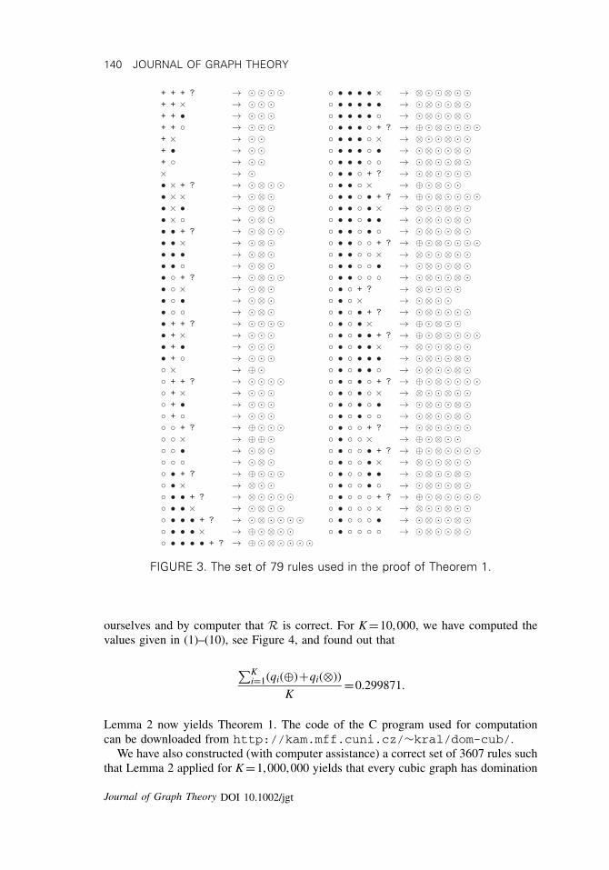
We apply Lemma 2 for a suitable correct set R of rules. This set of 79 rules canbe found in Figure 3; we have generated this set of rules by hand and checked both



FIGURE 3. The set of 79 rules used in the proof of Theorem 1.

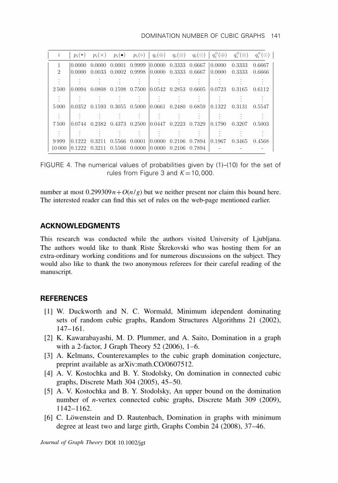
ourselves and by computer that R is correct. For K =10,000, we have computed thevalues given in (1)–(10), see Figure 4, and found out that

∑Ki=1(qi(⊕)+qi(⊗))

K=0.299871.

Lemma 2 now yields Theorem 1. The code of the C program used for computationcan be downloaded from http://kam.mff.cuni.cz/∼kral/dom-cub/.

We have also constructed (with computer assistance) a correct set of 3607 rules suchthat Lemma 2 applied for K =1,000,000 yields that every cubic graph has domination



FIGURE 4. The numerical values of probabilities given by (1)–(10) for the set ofrules from Figure 3 and K =10,000.

number at most 0.299309n+O(n /g) but we neither present nor claim this bound here.The interested reader can find this set of rules on the web-page mentioned earlier.

ACKNOWLEDGMENTS

This research was conducted while the authors visited University of Ljubljana.The authors would like to thank Riste Skrekovski who was hosting them for anextra-ordinary working conditions and for numerous discussions on the subject. Theywould also like to thank the two anonymous referees for their careful reading of themanuscript.

REFERENCES

[1] W. Duckworth and N. C. Wormald, Minimum idependent dominatingsets of random cubic graphs, Random Structures Algorithms 21 (2002),147–161.

[2] K. Kawarabayashi, M. D. Plummer, and A. Saito, Domination in a graphwith a 2-factor, J Graph Theory 52 (2006), 1–6.

[3] A. Kelmans, Counterexamples to the cubic graph domination conjecture,preprint available as arXiv:math.CO/0607512.

[4] A. V. Kostochka and B. Y. Stodolsky, On domination in connected cubicgraphs, Discrete Math 304 (2005), 45–50.

[5] A. V. Kostochka and B. Y. Stodolsky, An upper bound on the dominationnumber of n-vertex connected cubic graphs, Discrete Math 309 (2009),1142–1162.

[6] C. Lowenstein and D. Rautenbach, Domination in graphs with minimumdegree at least two and large girth, Graphs Combin 24 (2008), 37–46.



[7] M. Molloy and B. Reed, The dominating number of a random cubic graph,Random Structures Algorithms 7 (1995), 209–221.

[8] D. Rautenbach and B. Reed, Domination in cubic graphs of large girth,In: Proceedings of CGGT 2007, Lecture Notes in Computer Science 4535,Springer, Berlin, 2008, pp. 186–190.

[9] B. Reed, Paths, stars and the number three, Combin Prob Comput 5 (1996),267–276.

[10] N. C. Wormald, private communication, 2009.


Documents

Domination number of cubic graphs with large girth