DISCUSSION PAPER SERIES

IZA DP No. 12477

Sebastian FehrlerMaik T. Schneider

Buying Supermajorities in the Lab

JULY 2019

Any opinions expressed in this paper are those of the author(s) and not those of IZA. Research published in this series may include views on policy, but IZA takes no institutional policy positions. The IZA research network is committed to the IZA Guiding Principles of Research Integrity.The IZA Institute of Labor Economics is an independent economic research institute that conducts research in labor economics and offers evidence-based policy advice on labor market issues. Supported by the Deutsche Post Foundation, IZA runs the world’s largest network of economists, whose research aims to provide answers to the global labor market challenges of our time. Our key objective is to build bridges between academic research, policymakers and society.IZA Discussion Papers often represent preliminary work and are circulated to encourage discussion. Citation of such a paper should account for its provisional character. A revised version may be available directly from the author.

Schaumburg-Lippe-Straße 5–953113 Bonn, Germany

Phone: +49-228-3894-0Email: publications@iza.org www.iza.org

IZA – Institute of Labor Economics

DISCUSSION PAPER SERIES

ISSN: 2365-9793

IZA DP No. 12477

Buying Supermajorities in the Lab

JULY 2019

Sebastian FehrlerUniversity of Konstanz and IZA

Maik T. SchneiderUniversity of Bath

ABSTRACT

IZA DP No. 12477 JULY 2019

Buying Supermajorities in the Lab*

Many decisions taken in legislatures or committees are subject to lobbying efforts. A

seminal contribution to the literature on vote-buying is the legislative lobbying model

pioneered by Groseclose and Snyder (1996), which predicts that lobbies will optimally form

supermajorities in many cases. Providing the first empirical assessment of this prominent

model, we test its central predictions in the laboratory. While the model assumes sequential

moves, we relax this assumption in additional treatments with simultaneous moves. We

find that lobbies buy supermajorities as predicted by the theory. Our results also provide

supporting evidence for most comparative statics predictions of the legislative lobbying

model with respect to lobbies’ willingness to pay and legislators’ preferences. Most of these

results carry over to the simultaneous-move set-up but the predictive power of the model

declines.

JEL Classification: C92, D72

Keywords: legislative lobbying, vote-buying, Colonel Blotto, multi-battlefield contests, experimental political economy

Corresponding author:Sebastian FehrlerUniversity of KonstanzBox 13178457 KonstanzGermany

E-mail: sebastian.fehrler@uni-konstanz.de

* We would like to thank Carl Müller-Crepon for excellent research assistance and Alessandra Casella, Fabian Dvorak,

Urs Fischbacher, Moritz Janas, Gilat Levy, Simeon Schudy, Irenaeus Wolff and participants at several workshops and

conferences for valuable comments. All remaining errors are our own. This work was supported by Swiss National

Science Foundation grant 100017 150260/1.

1 Introduction

Special-interest groups frequently try to influence political decisions. The Center for Respon-

sive Politics documented that in just the first three quarters of 2017, lobbyists working on

tax-related issues donated USD 9.6 million to members of the U.S. Congress.1 A prominent

theoretical approach to analyze how such payments are made to influence political decisions

is the legislative lobbying model pioneered by Groseclose and Snyder (1996), henceforth GS.

However, the context of political decision making is just one where the model has been used.

More generally, it can represent many collective action problems in which two opposing actors

compete for support of a decision-making body by investing resources, such as money or effort,

to influence its members. Examples of such decision-making bodies include executive boards

in companies and committees in charge of monetary policy, hiring or common land-ownership

decisions, and many more. In the model, two opposed lobbies move once and sequentially. A

central prediction is that the first-moving lobby will often find it cheaper to win over a su-

permajority of legislators rather than a simple majority. Further, the model predicts that the

first-moving lobby should leave no soft spots for the opposed second-moving lobby by making

bribes so that all lobbied legislators are equally expensive to buy out of the coalition.

In this paper, we aim to shed some light on the predictive power of this prominent workhorse

model by testing its key predictions in the laboratory. Based on examples given in the original

GS paper, we design several scenarios with seven legislators predicting different sizes of lobbied

supermajorities and varying distributions of bribe offers. While the GS model provides clear

predictions and can represent many collective decision with lobby influence well, it has also

been criticised for the assumption of lobbies moving sequentially.2 For example, Grossman and

Helpman (2001) argue for simultaneous moves as they see no compelling reason for why lobbies

would be bound to a sequential protocol.3 In fact, there is also a large literature on lobbying

where lobbies move simultaneously.4 Therefore in a next step, we relax the assumption of

1We note that the Republican tax reform passed Congress in the fourth quarter. Seehttps://www.opensecrets.org/news/2017/12/tax-lobbyists-contributions for more details. Details on many morecases, almost exclusively based on data provided by the U.S. government, are presented on OpenSecrets.org,the Center for Responsive Politics’ website.

2Groseclose and Snyder (1996, p. 304) argue that sequential moves accord well with coalition building forexample when the status quo is a favored alternative. Then any proposed bill must beat the status quo and thelobby in favor of policy change needs to move first while the defender of the status quo can react and effectivelymove last. Another example given by GS is when coalitions need to be maintained over several sessions of thelegislature, where groups that oppose the bill may have opportunities to counterattack.

3 Grossman and Helpman (2001, p. 302) argue that “to impose a sequence of moves seems artificial here.Why should one special interest group have the ability to preempt the other in making offers to the legislators?What is to stop the other group from approaching the legislators at the same time? ” and that “the sequencingof offers in a model of legislative influence introduces unjustifiable restrictions on the groups’ political efforts.”.

4For example, there are large literatures on the Common agency lobbying model based on the approachadvanced by Bernheim and Whinston (1986) and Grossman and Helpman (1994), on lobbying contests withsimultaneous moves and on the Colonel Blotto game. We discuss these strands of the literature in more detailin the section where we relate our paper to the literate.

2

sequential moves and run treatments in which lobbies move simultaneously. Our study thus

combines tests of game-theoretical model predictions with a “stress test”.5

At first sight, it seems that moving from sequential to simultaneous moves could drastically

alter the logic of the game, as no lobby enjoys a second-mover advantage anymore. However,

despite the fact that no analytical predictions are available for the simultaneous case with

seven legislators, we argue that the underlying economic logic suggests that we should observe

similar comparative statics results with respect to the majority sizes as in the sequential case.

To be able to make more precise predictions for the simultaneous scenarios, we reduce the

number of legislators to three in additional treatments. While the computation of all equilibria

is unfeasible with normal computing power for the seven-legislators case, we are able to de-

termine all equilibria of the simplified set-up. In fact, for one scenario we obtain 56 different

(mixed-strategy) equilibria. However, they share some common properties, which allows for

comparative statics predictions regarding the number of bribes and the sum of bribes offered

between scenarios and, as conjectured, these predictions go in the same direction as those for

the sequential case. While it seems unlikely that these equilibria will be identified by the sub-

jects of the experiment, the comparative statics predictions might, nevertheless, capture the

economic intuition of the game. We compare the predictive performance of these equilibria

with the GS predictions for the sequential-moves case.

In the experiment, we focus on the behavior of the lobbies and hard-wire the behavior of

the legislators. Our experimental results confirm most comparative statics predictions of the

GS model for the sequential-moves scenarios, but point predictions regarding the number and

level of bribes are not very accurate. The explanatory power of the predictions derived in the

sequential-move set-up declines for the simultaneous-moves treatments but many comparative

statics predictions are, nevertheless, robust to the relaxation of this central model assumption.

The simplified scenarios with three legislators confirm this pattern.

Relation to the literature There are several different approaches to theoretically capturing

lobbying in the form of vote-buying.6 In the common-agency approach, several principals

(lobbies) make offer schedules to an agent (politician) specifying for any possible policy choice

how many resources they would pay if it was implemented. This model was introduced by

Bernheim and Whinston (1986) and it has often been applied since, for example, famously for

analyzing the role of special-interest groups in the shaping of trade policies (Grossman and

Helpman, 1994, 2001). Kirchsteiger and Prat (2001) test some of the model’s key predictions

5Morton and Williams (2010, p. 204) define a stress test as an investigation that tests “the predictions ofa formal model while explicitly allowing for one or more assumptions underlying the empirical study to be atvariance with the theoretical assumptions.” This approach is not very common in the experimental economicsliterature. A notable exception is the work on legislative bargaining by Tremewan and Vanberg (2016).

6For brevity we omit a discussion of other forms of lobbying, such as informational lobbying (Crawford andSobel, 1982) and lobbying in the form of legislative subsidies (Hall and Deardorff, 2006; Ellis and Groll, 2017).

3

in the lab.

While the common agency approach offers explanations of the lobbying of a single policy-

maker, our interest in this paper is in the lobbying of legislatures or committees. We focus

on the seminal legislative lobbying model of Groseclose and Snyder (1996). In the original

set-up, lobbies move sequentially in making offers to the legislators in favor of their preferred

policy choice, which is either an exogenously given policy change or the status quo. As one of

the landmarks in the lobbying literature the GS model has triggered interesting variations and

extensions (e.g., Diermeier and Myerson, 1999; Banks, 2000; Dekel et al., 2008, 2009; Hummel,

2009; Le Breton and Zaporozhets, 2010; Schneider, 2014, 2017) but surprisingly has not been

tested empirically in the laboratory. This is the focus of the present paper. In addition to testing

the model’s key predictions, we conduct a stress test by relaxing the central assumption of

sequential and publicly visible moves of the two lobbies. These somewhat arbitrary assumptions

have been a point for criticism of the sequential legislative lobbing model (e.g., in Grossman and

Helpman, 2001; see footnote 3). Assuming simultaneous moves instead – an equally arbitrary

assumption, proponents of the legislative lobbying model might argue – transforms the game

into a Colonel Blotto type of game. This class of games has been studied in another strand of

the literature.

The models proposed in this strand of the literature assume simultaneous moves. A contest

success function determines who wins the vote of a legislator in a legislature that is deciding

on an exogenously given policy proposal. Variations of this approach range from assuming

Tullock success functions to different types of auctions (e.g., Szentes and Rosenthal, 2003a,b;

Konrad and Kovenock, 2009; Kovenock and Roberson, 2012). The use of all-pay auctions has

been very prevalent in the theoretical literature. Various versions of all-pay auction lobbying

games have been studied in the laboratory (e.g., Arad and Rubinstein, 2012; Chowdhury and

Kovenock, 2013; Dechenaux et al., 2015; Hortala-Vallve and Llorente-Saguer, 2015; Montero

et al., 2016; Mago and Sheremeta, 2017). Of particular interest is the classical “Colonel Blotto

game”, first analyzed by Borel (1921), where the lobby making the highest payment wins the

legislator’s vote. The theoretical solutions to this game are notoriously complicated (Roberson,

2006; Roberson and Kvasov, 2012; Kvasov, 2007). Typically, no pure-strategy equilibria exist

in this class of games with the exception of some special cases, for example, with asymmetric

battlefield valuations (Hortala-Vallve and Llorente-Saguer, 2012). Casella et al. (2017) show

how decision-making with storable votes can be understood as a decentralized Blotto game –

decentralized, as voters with majority and minority preferences make their voting decisions in

a decentralized rather than in a coordinated way. The authors show that the economic logic

underpinning this game is very similar to that in Blotto games, where players have to mix

between the strategies of concentrating their votes on one issue or spreading them out over

several or even over all issues.

4

The simultaneous version of the model in our paper differs from Blotto games in that it is

not an all-pay auction. Lobbies make bribe offers that have to be paid only if the legislator votes

accordingly: that is, if the battlefield is won. However, our model shares the described economic

logic, according to which the weaker lobby tends to concentrate their bids on a few legislators

while the stronger lobby is more likely to spread its bids over a large number of legislators.

While there is no general theoretical solution of this particular game, we are able to present

results for some specific settings that we implement in the lab, and the experiment provides a

first idea of how different the results between the simultaneous and sequential variants are.

The paper is organized as follows. In Section 2, we introduce the sequential legislative

lobbying game and the theoretical reasoning behind its central equilibrium predictions. We

then discuss the game with simultaneous moves and explain why some comparative statics in

the simultaneous-move game may be similar to those in the sequential set-up. We go on to

design the scenarios that we implement in the lab and describe the procedural details of the

experiment. We present and discuss our results in Section 3 and we conclude in Section 4.

Experimental instructions and additional results are relegated to the Appendix.

2 Theoretical Background and Experimental Design

In this section, we first introduce the legislative lobbying model and its main theoretical pre-

dictions. We start with the sequential-move game and then discuss the differences for the

simultaneous-move game. Our focus will be on the intuition behind the theoretical results that

are important for our experiment.7 In the second part of this section, we explain the design of

the scenarios that we implement in the lab.

2.1 Theoretical Mechanism

The model set-up considers a legislature of size N that is to decide between the status quo

s and a new policy x by majority rule. We assume N to be an odd number for simplicity.

Legislators have preferences regarding the two policy options expressed by a bias vi in favor of

voting for the policy change and against the status quo. Legislators are referred to by subscript

i, i = 1, .., N .8 Two lobbies, A and B compete by making payment offers to legislators for votes

to win a majority in the legislature. Lobby A prefers policy change x over status quo s while

Lobby B supports the status quo s over x.9 We denote Lobby A’s and Lobby B’s maximal

7A more general theoretical analysis can be found in for example, Groseclose and Snyder (1996); Le Bretonand Zaporozhets (2010); Schneider (2014).

8The legislators’ biases vi can be micro-founded via sincere voting and utility functions ui(·) over <, aone-dimensional policy space, where x, s ∈ < and vi = ui(x)− ui(s).

9Hence, a positive value of a legislator’s bias vi expresses a preference in line with that of Lobby A, while anegative value vi shows alignment with the preferences of Lobby B.

5

willingness to pay for their preferred alternative by WA ≥ 0 and WB ≥ 0, respectively.10 We

will also refer to WA and WB as Lobby A’s and Lobby B’s prize for winning a majority for their

preferred policy.

In the sequential game, Lobby A moves first, offering a schedule of bribes {bAi }Ni=1 to the

legislators for a vote in favor of policy change. Lobby B moves second with schedule {bBi }Ni=1

for a vote for the status quo. Offers cannot be negative bAi , bBi ≥ 0. Lobbies only pay what they

offered if the legislator votes for their preferred alternative. After observing both lobbies’ offer

schedules, the legislators vote in favor of policy change if vi + bAi > bBi and otherwise they vote

for the status quo. The policy alternative that wins a majority will then be implemented. Note

that legislators get utility from voting for their preferred policy, irrespective of the legislature’s

decision to implement either of the two policy options.

Predictions in the sequential legislative lobbying game and economic intuition

For a given prize for Lobby B, WB, and given preference biases of the legislators, vi, there

exists an amount CA which is the smallest amount Lobby A will have to spend in payments

to legislators to form a majority coalition that cannot be broken by the opposed Lobby B

when moving second. Groseclose and Snyder (1996) show that there is a unique subgame-

perfect equilibrium for this sequential game, with the following property: If the first mover’s

willingness to pay for policy change x is larger than the amount necessary to form a winning

majority coalition, i.e. if WA ≥ CA, Lobby A will spend CA in the optimal way to form a

coalition that preempts the second mover from winning the vote and the second mover will

not make any payments. However, if WA < CA, the first mover Lobby A has no possibility

of keeping the second mover from securing a majority for the status quo and, hence, refrains

from offering any payments at all. The second mover will then only compensate the pro-change

biases of a sufficient number of legislators to form a simple majority for the status quo.

In fact, in all scenarios that we implement in the lab, a majority of legislators have a

(slight) preference bias for the status quo. Consequently, the second mover will never make any

payments in equilibrium and only the first mover will form winning coalitions through payments

if feasible. The following theoretical predictions and economic intuition for the sequential

lobbying game concern the optimal offer strategies of the first mover Lobby A to form a winning

coalition in the least expensive way. While we focus on the economic intuition behind the

equilibrium properties in the main text, in Appendix A, we provide a formal discussion, which

we also relate to the specific scenarios we test in the laboratory.

The equilibrium properties provide four key predictions that we will test in the laboratory.

First, there are no scenarios in which both lobbies make payments. Second, when

10The lobbies’ willingness to pay can be micro-founded similarly to the legislators’ biases in footnote 8by defining the lobbies’ utility functions Uj(·), j = A,B, over <, with WA = UA(x) − UA(s) and WB =UB(s)− UB(x).

6

making payments, the first-mover lobby will use a leveling strategy, where every bribed

legislator will be equally expensive to buy back for the second mover. The intuition for the

optimality of a leveling strategy is that it leaves no “soft spots”. To understand this, suppose

that some legislators can be bought back by the second mover at a lower expense than others.

Requiring only a simple majority for the status quo to destroy the coalition for a policy change,

the most expensive legislators will not be offered any payments – the second mover will instead

concentrate his offers on the cheapest set of legislators. In this case, however, it is optimal for

the first mover to reduce the offers to the most expensive legislators to increase the offers to

the least expensive ones. This logic applies as long as the legislators differ in regard to the cost

of securing their vote in the second mover’s favor.

The third central prediction is that the optimal sizes of the majorities (weakly) de-

crease with the legislators’ biases in favor of the status quo, vi, and (weakly) in-

crease with the prize for B, WB. The central insight advanced by Groseclose and Snyder

(1996) is that it is often cheaper to form a supermajority than a simple majority. The key

intuition behind this insight is that the amount necessary for the second mover to destroy a

majority formed by the first mover must exceed the second mover’s willingness to pay, WB. In

the case of a simple majority, the second mover needs to buy back only one legislator. That is,

for each legislator in the first-mover’s coalition, the first mover’s offer bAi minus the legislator’s

initial bias for the status quo vi must be larger than the second mover’s willingness to pay,

WB. If the first mover increased the majority by another legislator, the second mover needs to

buy back two legislators to break the coalition for a policy change. Consequently, for any two

legislators the cost must exceed the second mover’s willingness to pay. This allows the first

mover to reduce the offers made to each single legislator, thereby saving resources as long as

the initial status quo bias of the additional legislator in the coalition is sufficiently small. The

trade-off when including another legislator in the coalition is between the resources that can

be saved by being able to reduce the bribe offers to all other legislators in the coalition and

the extra amount to be paid to neutralize this legislator’s initial bias in favor of the status quo.

Accordingly, if the legislators do not have any preferential bias towards the status quo, it will

be optimal to form a coalition including all legislators.11

Further, for given preference biases of the legislators, the larger the willingness to pay for

B, WB, is, the larger will be the reduction in the offers to the legislators in the coalition, when

the majority is increased by an additional legislator. Hence, ceteris paribus, the larger B’s

willingness to pay is the (weakly) larger the size of Lobby A’s majority will be. It follows from

this intuition that, ceteris paribus, if the legislators’ biases in favor of the status quo are smaller

or the second mover’s willingness to pay is larger, the size of the supermajority formed by the

first-mover will be larger.

11Formal arguments and examples are provided in Appendix A.

7

The fourth prediction is that, either Lobby A will win the vote for sure (if WA ≥ CA)

or Lobby B will win for sure (if WA < CA). Due to the unique pure-strategy equilibrium

there is no uncertainty as to which lobby will win the vote.

We test these predictions in the lab in several scenarios varying the degrees of the status-quo

biases of the legislators and the second mover’s prize which reflects their maximal willingness to

pay to break a pro-change majority by the first-mover lobby. We describe the specific scenarios,

with their particular predictions, in the next section.

Predictions in the simultaneous-move game and economic intuition

As discussed in the Introduction, one of the specific criticisms of the sequential legislative

lobbying model is the sequential timing of the lobbies’ moves. The direct method of assessing

how important the sequential moves are in this set-up is to compare the outcomes with those

in the exact same game but with simultaneous moves. Models of this type are often referred

to as “Colonel Blotto games”, which are notoriously difficult to solve analytically.12

Consequently, the only way to obtain theoretical predictions for our experiment is to com-

pute the equilibria for the particular scenarios and parameters that we bring into the laboratory.

For the standard legislative lobbying game, as described earlier, this is possible for the simplest

possible set-up with three legislators and very low willingness to pay WB = 1 on the part of

Lobby B defending the status quo. The two scenarios we bring to the lab and for which we

can compute the equilibria differ in the legisators’ preferences. In the first scenario, legislators

have a very weak bias against policy change towards x, vi = −0.5, while in the second scenario

they have stronger opposition to policy change with vi = −4.5. Even in this simplest set-up,

we obtain a large number of equilibria for the two scenarios that can be summarized in several

equilibrium types. We provide a discussion of all the equilibrium types in Appendix B and we

summarize some central characteristics of these equilibrium types in Table 2 in Section 2.2.

From the results, we observe that, first, in contrast to the case with sequential moves, we

expect that both lobbies will make positive payment offers in all scenarios, although

in most equilibrium types the probability placed by Lobby B on the pure strategy of not

offering any payments is very high. Second, in the simultaneous game the degree of persuing

leveling strategies varies between equilibrium types. Consequently we expect to observe a lower

12Except for trivial cases, for example when one lobby’s willingness to pay is zero, there cannot be anypure-strategy equilibria. The reason for this is the following: in any combination of two pure strategies byLobbies A and B, if one of the lobbies wins there will be a possibility to deviate to win at lower costs given thestrategy of the other lobby, or there is a possibility for the other lobby to win the majority given its opponent’soffer schedule. While several variants of these “Colonel Blotto games” have been solved, resulting in verycomplicated mixed-strategy equilibria, there is no general solution in the literature that could be easily adaptedto our simultaneous-move set-up because of two particular properties: (1) it is not an all-pay auction: offers donot have to be paid if the legislator does not vote accordingly; and (2) the lobbies’ objectives are to win themajority of votes, while the Colonel Blotto game has been solved for lobbies which try to maximize the numberof voters voting for their cause (not caring about whether they will win a majority).

8

frequency of leveling strategies in the simultaneous relative to the sequential game

set-up. Our greatest interest is in whether supermajorities will be observed in the simultaneous

game as well and how the optimal coalition size will change with the legislators’ preferences and

Lobby B’s willingness to pay. In our set-up with three legislators we predict supermajorities in

the case with very low intensities of preferences of the legislators. Moreover as in the sequential

move game, the expected size of the majority declines with the legislators’ biases in favor of

the status quo. Unfortunately, it is not possible to derive equilibrium predictions for more

complicated set-ups, with more than three legislators or higher willingness to pay for the status

quo with normal computing power.13 However, the following intuition suggests that a similar

logic regarding supermajorities as in the sequential game holds in the simultaneous-move game

as well.

In principle, there are two strategy types for winning a majority: (a) offering a large num-

ber of legislators a small amount on top of neutralizing the legislators’ preference biases and

(b), offering a smaller number of legislators a substantial amount on top of preference bias

neutralization. Strategy (a) tries to win a majority by winning over those legislators to which

the opposed Lobby B did not make any offers or offered very little. Overall, the probability

of winning the vote of any particular legislator might not be very high but the probability of

winning sufficient legislators for a majority is substantial. Strategy (b) seeks to achieve a high

probability of winning almost all of the legislators in a small coalition. The mixed strategies of

the lobbies in the simultaneous game are probability distributions over the support comprising

strategies of type (a) and type (b) as well as hybrid versions of the two. If the preference of

the legislators is biased more strongly against the policy change, Lobby A needs to pay more

to neutralize the preference bias for all legislators in its coalition. This makes strategies of

type (a) more costly and we expect that this will reduce the probability weight on such pure

strategies in the mixed strategy played in equilibrium. Consequently, as in the sequential game,

we predict that the expected size of the majorities formed by Lobby A will be smaller if the

legislators’ preference biases against the policy change are larger. By contrast, if the prize of

winning the vote for Lobby B increases, securing almost all legislators’ votes in a small coali-

tion will become substantially more expensive for A, leading to a reduction in the probability

weight on strategies of type (b). Hence, we expect larger expected majority sizes for A if B’s

willingness to pay is higher.

The depicted intuition suggests that the optimal sizes of the majorities (weakly)

decrease with the legislators’ biases in favor of the status quo, vi, and (weakly)

increase with the prize for B, WB. Consequently, we expect the comparative statics of the

coalition sizes with respect to preference biases and the prize for B to be qualitatively the same

13For example, with seven legislators and a willingness to pay of Lobby A of 9, there are roughly 107 (notweakly dominated) pure strategies for Lobby A. The payoff matrix would be extremely large (many terabytes).

9

as in the sequential game.

Finally, while in the sequential game lobbies either win or lose the vote for sure, the simul-

taneous game allows Lobby A to slightly reduce the probability of winning in order to reduce

the expected amount of bribes to be paid. This is what we can observe for the three legislator

case in Table 2. Hence, we expect that the winning probability of A will be lower in

the simultaneous game than in the sequential legislative lobbying game and that

Lobby B’s winning probability is positive.

While the scenarios with the three legislators set-up allows to derive theoretical predictions

for both the sequential and simultaneous-move game, this is not possible for the scenarios with

more legislators. However, it is still interesting to see if the intuition and predictions outlined

above for the three legislator case also show up in scenarios with more than three legislators.

For this reason, we bring two different set-ups, each with sequential and simultaneous moves,

into the laboratory: one with seven legislators and one with three. The scenarios with seven

legislators allow us to directly connect to the examples for the sequential move games given

in Groseclose and Snyder (1996) and to test how different the outcomes will be if the game is

played with simultaneous moves.

2.2 Lab Scenarios

In the experiment, we implement seven scenarios for the game with seven legislators and two

scenarios for the game with three legislators.

In the first five scenarios with seven legislators, all legislators are identical and between

scenarios we vary their preference bias towards the status quo as well as Lobby B’s willingness

to pay. In the last two scenarios with seven legislators, we slightly increase the complexity by

considering differences in the preferences of the legislators and by varying the willingness to

pay of the status quo-defending lobby between the two scenarios.

For the set-up with three legislators, we consider two scenarios with homogeneous legislators

with different status-quo biases between the two specifications. As indicated previously, our

focus here is on testing our theoretical predictions for both the simultaneous and the sequential

games.

2.2.1 Legislature with Seven Legislators

In all scenarios, Lobby A possesses a maximal willingness to pay of 300 in order to win the

vote in favor of a policy change. Lobby B’s willingness to pay to win the vote for preserving

the status quo varies between a relatively weak 12, a strong preference of 60, and a very strong

preference of 180. Moreover, the scenarios show different biases of the legislators. In the

sequential games, Lobby A always moves first, and the defender of the status quo, B, moves

10

second. The budgets are 400 for Lobby A and 200 for Lobby B.

Scenarios with homogeneous legislator preferences We consider legislators to be either

unbiased (more precisely, they have a minimal bias of 0.5 in favor of the status quo as a tie

breaker if no payments are made), or to have a strong status quo bias of 19.5. The particular

scenarios with their equilibrium predictions in the sequential-move game are summarized in

Table 1.

Table 1: Theoretical Predictions for Scenarios with Seven Legislators

Sc1 Sc2 Sc3 Sc4 Sc5 Sc6 Sc7

Prize B, WB 12 12 60 60 180 12 60Legislator valuationLegislators 1–3 - 0.5 -19.5 -0.5 -19.5 -19.5 12.5 12.5Legislators 4–7 - 0.5 -19.5 -0.5 -19.5 -19.5 -19.5 -19.5

Equilibrium predictionsCoalition size A 7 4 7 6 0 4 6

Leveling [%] 100 100 100 100 0 100 100

Total bribes A, CA 25 128 109 238 0 32 142

Total bribes B 0 0 0 0 0 0 0

The idea behind Scenarios 1–4 is to test our hypotheses regarding the predictions on changes in

the prize for Lobby B and in the legislators’ evaluations. In particular, comparing the results

between Scenarios 1 and 2, and between Scenarios 3 and 4, indicates the effects of differences

in the legislators’ preference biases towards the status quo. With higher biases the majority is

predicted to decline. The majority size declines less if the value of the status quo for Lobby B

is higher as the latter makes a larger majority more beneficial as explained in Section 2.1.

Comparing the results between Scenarios 1 and 3, and between Scenarios 2 and 4, reveals

whether the hypothesis that majority sizes (weakly) increase with higher willingness to pay of

the status quo defender holds. As pointed out previously, with neutral bias of the legislators it

is always optimal to form a maximal coalition including the entire legislature. However, there

are substantial costs of large majorities when the legislators have strong status-quo biases. In

this case, a large coalition is only optimal for the pro-change lobby if the defender of the status

quo has a high willingness to pay, thereby increasing the benefits of a large supermajority.

In Scenario 5, we test the case where the willingness to pay by Lobby B is so high that

there is no profitable way for Lobby A to preempt Lobby B buying back a sufficient number of

legislators to preserve the status quo.

The theory predicts leveling in all cases (except Scenario 5), which theoretically implies

that all legislators in the coalition obtain the same offer in the scenarios with homogeneous

11

legislator valuations. As we only allow offers in integers in the experimental scenarios and

impose valuations of a half to break ties, the least expensive way to form a majority coalition

for Lobby A is to pay one unit less to one legislator less the number of legislators in the coalition

that the second mover needs to buy back to destroy the majority in favor of policy change.

As a consequence of the indivisibility implied by integer offers, leveling in the scenarios we

implement in the lab can thus include differences of one between the offers.

Heterogeneous valuations by legislators We also test the situation where the legislators

have heterogeneous valuations. Three legislators have valuation 12.5 in favor of policy change

and four legislators have −19.5. The prize of winning for B is again either 12 or 60. In the

case where Lobby B’s willingness to pay is only 12, Lobby A does not have to worry about B

offering bribes to any of the three legislators with 12.5 valuation of policy change when it forms

a winning coalition. Consequently, Lobby A will concentrate their offers on the legislators that

are biased towards the status quo to form a pro policy change coalition that includes legislators

with and without bribe offers. This is referred to as a non-flooded coalition, following GS’s

terminology. In the second case, where B’s willingness to pay is 60 for the status quo, it is

necessary to make an offer to a legislator with initial preference bias of 12.5 in favor of policy

change. As a consequence of the “leaving no soft spots” logic, Lobby A will have to make

additional offers to the pro-change legislators as well as to a number of legislators initially

leaning towards the status quo. All legislators in the formed coalition will receive payments: a

flooded coalition.

Scenarios 6 and 7 have been set-up to test whether participants form a non-flooded and a

flooded coalition, respectively. In Scenario 6, it is optimal for Lobby A to form a non-flooded

coalition of four where only one pro status-quo legislator with valuation −19.5 receives a bribe

of 32. In Scenario 7, it is optimal for A to form a flooded coalition with six legislators. To

make all legislators in the coalition equally costly to buy back, Lobby A offers all pro-change

legislators a payment of 8 and among the other three status-quo leaning legislators it offers 39

to two of them and 40 to one. Recall that the latter is due to our design, which allows only

integers as payment offers. The minimal total cost for this flooded coalition will be 142.

2.2.2 Legislature with Three Legislators

Both lobbies possess a budget of 30. The maximal willingness to pay for policy change by

Lobby A is 25 and the maximal willingness to pay to defend the status quo by Lobby B is 2.

Legislators are homogeneous and we again implement a scenario (Scenario 1) where legislators

are unbiased (valuation of −0.5 for tie-break without payments) and one where they relatively

strongly lean towards the status quo −4.5 (Scenario 2).

In the sequential game, where Lobby A moves first, it is least expensive to buy a super-

12

majority comprising all three voters and to spend 2 on two legislators and offer 1 to the third,

summing up to a total cost of 5. In Scenario 2, the costs of a vote in favor of policy change

is more expensive, leading to an optimal majority of two legislators formed by paying both 7.

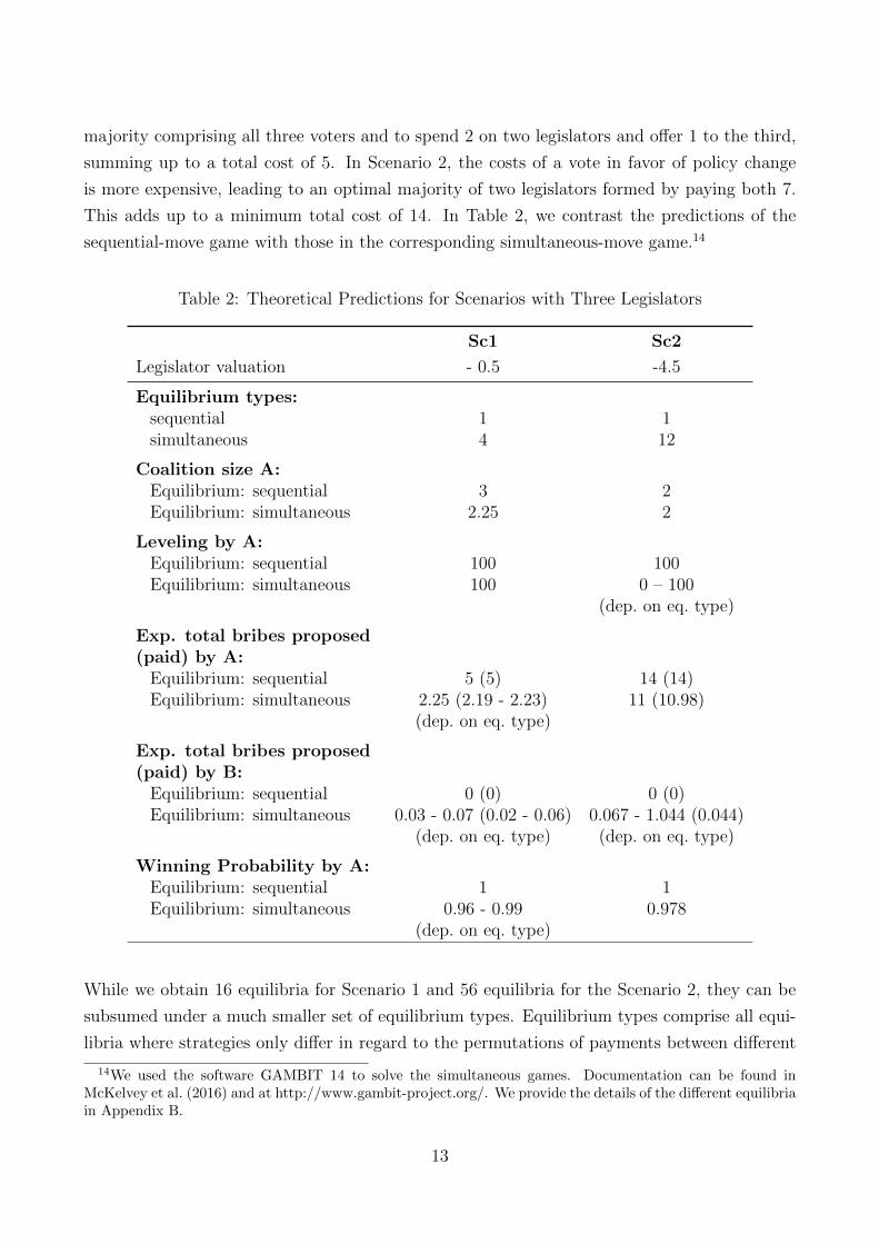
This adds up to a minimum total cost of 14. In Table 2, we contrast the predictions of the

sequential-move game with those in the corresponding simultaneous-move game.14

Table 2: Theoretical Predictions for Scenarios with Three Legislators

Sc1 Sc2

Legislator valuation - 0.5 -4.5

Equilibrium types:sequential 1 1simultaneous 4 12

Coalition size A:Equilibrium: sequential 3 2Equilibrium: simultaneous 2.25 2

Leveling by A:Equilibrium: sequential 100 100Equilibrium: simultaneous 100 0 – 100

(dep. on eq. type)

Exp. total bribes proposed(paid) by A:

Equilibrium: sequential 5 (5) 14 (14)Equilibrium: simultaneous 2.25 (2.19 - 2.23) 11 (10.98)

(dep. on eq. type)

Exp. total bribes proposed(paid) by B:

Equilibrium: sequential 0 (0) 0 (0)Equilibrium: simultaneous 0.03 - 0.07 (0.02 - 0.06) 0.067 - 1.044 (0.044)

(dep. on eq. type) (dep. on eq. type)

Winning Probability by A:Equilibrium: sequential 1 1Equilibrium: simultaneous 0.96 - 0.99 0.978

(dep. on eq. type)

While we obtain 16 equilibria for Scenario 1 and 56 equilibria for the Scenario 2, they can be

subsumed under a much smaller set of equilibrium types. Equilibrium types comprise all equi-

libria where strategies only differ in regard to the permutations of payments between different

14We used the software GAMBIT 14 to solve the simultaneous games. Documentation can be found inMcKelvey et al. (2016) and at http://www.gambit-project.org/. We provide the details of the different equilibriain Appendix B.

13

legislators. In all four equilibrium types in Scenario 1, the pro-change Lobby A randomizes

between a grand coalition with payments of 1 for each legislator, and forming simple majorities

by offering a payment of 1 to any two legislators. Each of the four possibilities carries an equal

probability weight of 0.25. Consequently, we expect a supermajority in a fourth of cases and in

three-quarters of cases a simple majority. This implies that, on average, coalition sizes formed

by A should be 2.25 and the expected costs amount to 2.25 as well. Compared to the sequential

set-up, this makes it substantially cheaper for Lobby A to effect policy change, which reflects

the second-mover advantage of the defender of the status quo in the sequential set-up, as well

as the fact that it is optimal for the pro-change lobby to give up a 100% probability of winning

the vote. The different strategies by Lobby B define the four equilibrium types. However, they

look very similar: all place a large probability of about 95% on not making any offers, while

the six strategies where either one or two legislators are offered an amount of 1 carry almost

equal shares of the remaining 5% probability. Consequently, we expect, on average, close to

zero payments by Lobby B.

In Scenario 2, we find 12 equilibrium types. All equilibria have in common that the pro-

change Lobby A will form a minimal coalition of two legislators and all involve expected total

costs of 11.

These are clear predictions that we will test in the experiment. Comparing the two scenarios

in the simultaneous game, the average coalition size should be larger in Scenario 1 compared

to Scenario 2 and the amount spent to win the majority should be higher. Relative to the

sequential game, we expect to find smaller coalition sizes, less payments offered in total, and a

lower probability of winning the vote for Lobby A in the simultaneous game.

2.3 Procedural Details

To test the accuracy of our theoretical predictions with respect to the lobbies’ behavior, we

implemented the scenarios described above in four different treatments (sequential and simul-

taneous moves with three and seven legislators). A total of 162 students from ETH Zurich and

the University of Zurich (58% female, average age 23 years) participated in 10 experimental

sessions in the DeScil laboratory at ETH Zurich.15

In the 7-legislators sessions, participants played one round of each of the seven scenarios.

Before that, they played three practice rounds. The sequence of scenarios was varied randomly

between the sessions with sequential moves. For each session with a specific sequence in the

sequential-moves treatment, we also ran one with the same sequence in the simultaneous-moves

treatment. In the three-legislators sessions, subjects played five rounds of each of the two

scenarios in a row after two practice rounds. One of the two sessions in the two subtreatments

(sequential and simultaneous) started with Scenario 1, the other one with Scenario 2. In all

15The experiment was programmed in zTree (Fischbacher, 2007).

14

treatments, subjects were randomly re-matched after every round, and the roles of Lobby A and

Lobby B were also randomly assigned within each pair of matched subjects in every round. As

our focus is on the behavior of the lobbies, we chose to hardwire the behavior of the legislators

in the following way: each computerized legislator is programmed to vote for the alternative

that gives it the highest payoff.

Table 3: Number of Sessions and Participants

Seven legislators Three legislators

Seq Sim Seq Sim

Sessions 3 3 2 2Subjects 82 80 56 56

Notes: A session lasted on average 110 minutes and aver-age earnings were CHF 52.

In the beginning of each round, subjects were informed about their role as Lobby A or B (called

member A/B in the instructions) their corresponding budget and the legislators’ (committee

members’) valuations. On the second screen, they made their bids. At the end of every

round, they saw a feedback screen informing them about the legislators’ decisions and their

payoff. Subjects were paid a show-up fee of CHF 5 in addition to the points they earned in the

experiment, which were converted into Swiss Francs at an exchange rate of CHF 0.02/point

(CHF 0.13/point) in the sessions with seven (three) legislators.

Subjects were informed about all these details in the instructions and we checked their

understanding with an on-screen quiz before the start of the experiment (see Appendix D for

the instructions and the quiz).

3 Experimental Results

3.1 Seven Legislators

Table 5 summarizes the descriptive statistics for all scenarios. Figures 1 (C1) and 2 (C2) give

a graphical overview of the behavior of Lobbys A (B), and Table 4 (C1) shows the comparative

statics results for the sequential (simultaneous) scenarios.

3.1.1 Number and Level of Bribes

Sequential moves Starting with Scenarios 1–5, we observe that the comparative statics

predictions with respect to the bias of the legislators hold in the data (Figure 1 and Table 4).

15

However, while the comparative statics prediction regarding the willingness to pay of Lobby B

holds for the comparison of Scenarios 1 and 3, it does not hold for the comparison of Scenarios

2 and 4. As we can see in the lower panel of Figure 1 this is driven by the roughly one third of

the Lobbies A who make zero bids.

Table 4: Comparative Statics 7 Legislators: Number of Bribes of Lobby A

Sc.1 Sc.2 Sc.3 Sc.4 Sc.5 Sc.6 Sc.7

Sc.1 < > < > > > >p-value .338 .032† .017† .000† .000 .000 .189

Sc.2 > < >∗ > > <p-value .941 .000 .036† .000 .000 .455

Sc.3 < > > > >p-value .008 .000† .000 .000 .000

Sc.4 > > > <p-value .018† .000 .037† .014†

Sc.5 < < <p-value .000 .000† .000

Sc.6 > <p-value .000 .000

Sc.7 >p-value .290

Notes:: > (<): average number of bribes in row scenario greater (smaller)

than column scenario; in the diagonal the scenario with sequential moves

is tested against the same scenario with simultaneous moves; all off-diagonal

comparisons are between sequential-moves scenarios; p-value are for two-sided

tests. ∗: direction is opposite to theoretical prediction; †: significant at 5%

with clustering at subject level but not with clustering at session level.

As shown in Table 4, this is the only difference between treatments which goes in the opposite

direction to the theoretical prediction. The point predictions with respect to number of bribes

by Lobby A are not very accurate and the observed means differ significantly from the predic-

tions in all five scenarios.16 However, regarding the distribution of number of bribes, the mode

corresponds to the theoretical prediction in all scenarios except Scenario 4, in which it is most

expensive but still profitable for A to win. Regressing the actual number of bribes offered on the

theoretically predicted number, reveals that the theoretically predicted values have a strongly

16In Scenarios 6–7, legislators’ valuations are not homogeneous and predictions are qualitatively different.We therefore analyze these scenarios separately. However, we also present the regression results of all scenarioscombined in Appendix C.

16

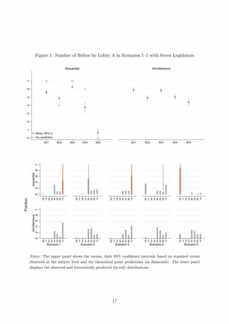
Figure 1: Number of Bribes by Lobby A in Scenarios 1–5 with Seven Legislators

01

23

45

67

Sc1 Sc2 Sc3 Sc4 Sc5

Mean, 95% ciEq. prediction

Sequential

Sc1 Sc2 Sc3 Sc4 Sc5

Simultaneous

0.2

.4.6

.81

sequ

entia

l

0 1 2 3 4 5 6 7 0 1 2 3 4 5 6 7 0 1 2 3 4 5 6 7 0 1 2 3 4 5 6 7 0 1 2 3 4 5 6 7

0.2

.4.6

.81

sim

ulta

neou

s

0 1 2 3 4 5 6 7Scenario 1

0 1 2 3 4 5 6 7Scenario 2

0 1 2 3 4 5 6 7Scenario 3

0 1 2 3 4 5 6 7Scenario 4

0 1 2 3 4 5 6 7Scenario 5

Frac

tion

Notes: The upper panel shows the means, their 95% confidence intervals based on standard errors

clustered at the subject level and the theoretical point predictions (as diamonds). The lower panel

displays the observed and theoretically predicted (in red) distributions.

17

Figure 2: Number of Bribes by Lobby A in Scenarios 6 and 7 with Seven Legislators

01

23

45

67

Sc6 Sc7

Mean, 95% ciEq. prediction

Sequential

Sc6 Sc7

Simultaneous0

.2.4

.6.8

1se

quen

tial

0 1 2 3 4 5 6 7 0 1 2 3 4 5 6 7

0.2

.4.6

.81

sim

ulta

neou

s

0 1 2 3 4 5 6 7Scenario 6

0 1 2 3 4 5 6 7Scenario 7

Frac

tion

Notes: The upper panel shows the means, their 95% confidence intervals based on standard errors clustered at

the subject level and the theoretical point predictions (as diamonds). The lower panel displays the observed

and theoretically predicted (in red) distributions.

18

Table 5: Results for Scenarios with Seven LegislatorsS

c1se

Sc2

seS

c3se

Sc4

seS

c5se

Sc6

seS

c7se

#Bribespropo

sedby

A:

Equ

ilib

riu

m:

sequ

enti

al

74

76

01

6O

bse

rved

:se

qu

enti

al

5.5

9(0

.18)

4.8

8(0

.14)

6.2

7(0

.12)

3.7

6(0

.33)

0.6

8(0

.21)

2.4

9(0

.21)

5.1

2(0

.19)

Ob

serv

ed:

sim

ult

an

eou

s5.9

(0.1

5)

4.9

(0.1

5)

5.8

3(0

.13)

5.0

3(0

.16)

4.4

(0.2

4)

4.6

(0.1

9)

4.7

5(0

.16)

#Bribespropo

sedby

B:

Equ

ilib

riu

m:

sequ

enti

al

00

00

00

0O

bse

rved

:se

qu

enti

al

0.5

6(0

.14)

0.4

4(0

.1)

0.9

8(0

.17)

0.3

2(0

.1)

0.4

4(0

.13)

0.2

7(0

.08)

1.2

2(0

.17)

Ob

serv

ed:

sim

ult

an

eou

s2.8

5(0

.31)

2.5

3(0

.29)

3.4

5(0

.28)

4.3

3(0

.23)

5.1

8(0

.18)

2.2

3(0

.24)

3.3

3(0

.23)

Voteswonby

A:

Equ

ilib

riu

m:

sequ

enti

al

74

76

04

6O

bse

rved

:se

qu

enti

al

5.2

(0.2

)4.5

4(0

.16)

5.3

4(0

.2)

3.4

4(0

.33)

0.3

7(0

.11)

4.3

2(0

.15)

4.4

9(0

.2)

Ob

serv

ed:

sim

ult

an

eou

s5.3

8(0

.2)

4.2

3(0

.2)

5.1

(0.1

8)

4.2

5(0

.19)

2.8

8(0

.24)

4.6

8(0

.16)

4.6

(0.1

6)

Awins(%

):E

qu

ilib

riu

m:

sequ

enti

al

100

100

100

100

0100

100

Ob

serv

ed:

sequ

enti

al

80.4

9(4

.4)

73.1

7(4

.92)

65.8

5(5

.27)

48.7

8(5

.55)

0(0

)75.6

1(4

.77)

48.7

8(5

.55)

Ob

serv

ed:

sim

ult

an

eou

s92.5

(2.9

6)

75

(4.8

7)

90

(3.3

8)

77.5

(4.7

)47.5

(5.6

2)

85

(4.0

2)

77.5

(4.7

)

Totalbribes

propo

sedby

A:

Equ

ilib

riu

m:

sequ

enti

al

25

128

109

238

032

142

Ob

serv

ed:

sequ

enti

al

69.2

7(6

.03)

148.6

8(6

.65)

126.4

6(6

.21)

141.4

1(1

3.5

1)

17.8

(5.4

3)

69.9

8(8

.12)

137.7

6(8

.82)

Ob

serv

ed:

sim

ult

an

eou

s98.8

(9.5

9)

137.6

8(8

.17)

118.5

8(8

.21)

162.0

5(7

.97)

122.0

8(1

0.5

6)

111.3

(8.1

7)

117.2

3(9

.43)

Totalbribes

propo

sedby

B:

Equ

ilib

riu

m:

sequ

enti

al

00

00

00

0O

bse

rved

:se

qu

enti

al

6.5

4(3

.43)

3.1

2(0

.66)

19

(3.2

1)

4.3

7(1

.45)

8.0

2(2

.65)

6.1

7(3

.43)

20.7

8(2

.83)

Ob

serv

ed:

sim

ult

an

eou

s16.2

(5.6

1)

15.9

8(4

.1)

21.2

8(4

.61)

33.3

(5.7

8)

78.3

3(6

.26)

22.5

3(5

.61)

28

(4.6

2)

Winningcoalitionsize

ifA

wins:

Equ

ilib

riu

m:

sequ

enti

al

74

76

46

Ob

serv

ed:

sequ

enti

al

5.8

2(0

.16)

5.1

3(0

.16)

6.5

6(0

.12)

6.1

5(0

.18)

XX

4.7

7(0

.16)

6.0

5(0

.2)

Ob

serv

ed:

sim

ult

an

eou

s5.7

6(0

.14)

5.0

7(0

.13)

5.4

7(0

.14)

4.9

4(0

.13)

4.7

9(0

.15)

5.0

6(0

.14)

5.1

(0.1

5)

Winningcoalitionsize

ifB

wins:

Equ

ilib

riu

m:

sequ

enti

al

7O

bse

rved

:se

qu

enti

al

4.3

8(0

.25)

4.0

9(0

.06)

4(0

)6.1

4(0

.21)

6.6

3(0

.11)

4.1

(0.0

7)

4(0

)O

bse

rved

:si

mu

ltan

eou

s6.3

3(0

.39)

5.3

(0.2

7)

5.2

5(0

.39)

5.1

1(0

.28)

5.8

6(0

.19)

4.5

(0.2

2)

4.1

1(0

.07)

Levellingby

A(%

):E

qu

ilib

riu

m:

sequ

enti

al

100

100

100

100

0100

100

Ob

serv

ed:

sequ

enti

al

87.8

8(5

.72)

90

(5.5

1)

85.1

9(6

.88)

100

(0)

0(0

)29.0

3(8

.21)

35

(10.7

4)

Ob

serv

ed:

sim

ult

an

eou

s29.7

3(7

.56)

40

(9)

36.1

1(8

.06)

45.1

6(9

)57.8

9(1

1.4

)0

(0)

9.6

8(5

.34)

Quasi-levellingby

A(%

):O

bse

rved

:se

qu

enti

al

93.9

4(4

.18)

93.3

3(4

.59)

88.8

9(6

.09)

100

(0)

0(0

)39.1

3(1

0.2

5)

70

(10.3

2)

Ob

serv

ed:

sim

ult

an

eou

s48.6

5(8

.27)

73.3

3(8

.13)

50

(8.3

9)

51.6

1(9

.03)

63.1

6(1

1.1

4)

18.7

5(6

.95)

32.2

6(8

.45)

Notes:

Sta

nd

ard

erro

rs(s

es)

are

clu

ster

edat

the

sub

ject

level

.L

ob

by

An

ever

win

sin

the

sequ

enti

al

set-

up

inS

cen

ari

o5.

Th

eref

ore

,w

eh

ave

no

ob

serv

ati

on

sof

win

nin

gco

aliti

on

size

sfo

rth

issc

enari

o(a

sin

dic

ate

dby

the

“X

”).

Lev

elin

gan

dqu

asi

-lev

elin

gre

fer

toth

est

rate

gy

typ

esas

defi

ned

in3.1

.2.

19

significantly positive coefficient and explain 42% of the variation across Scenarios 1–5 (Table

C2).17 While the total sum of bribes offered differs significantly from the point predictions

(Table 5), regressing the former on the latter, indicates that the theoretically predicted values

have a strongly significantly positive coefficient and explain 21% of the variation in the bribe

levels across Scenarios 1–5 (Table C3).

Turning to Scenarios 6 and 7 (Figure 1 and Table 5), we find that the point predictions are

again not accurate but the comparative statics prediction regarding the willingness to pay of

Lobby B is confirmed. Regressing the actual number of bribes and the total sum of bribes offered

on the theoretically predicted values we find that the latter are strongly significant predictors

of the observed behavior in the lab and explain 35% of the variation in both regressions (Tables

C2 and C3).

Lobby A does not always win when it should. In Scenarios 4 and 7, where winning is

most costly, it wins in only 49% of the cases (see Table 5). In the other scenarios, Lobby A

wins substantially more often. To a large extent the low winning rates are due to suboptimal

behavior on the part of Lobby A. However, in some cases Lobby B wins by paying more than

its willingness to pay. In Scenario 5, where A is predicted to lose, it does indeed always lose. As

illustrated graphically in Figures C1, C2, C5, and C6, Lobby B’s bids are mostly close to zero in

all seven scenarios, as predicted. However, while the median number and level of bribes is zero

in Scenarios 1-4 and 6-7 (see Figures C1, C2, C5 and C6) the means are strongly significantly

larger than zero in all scenarios.

Simultaneous moves Starting again with Scenarios 1–5, we observe a similar pattern re-

garding the comparative statics. However the differences between treatments with respect to

the average number of bribes and the total bribe level are less pronounced than in the sequen-

tial case (see Figure 1 and Table C1). When we regress the actual number of bribes offered

on the theoretically predicted number for the sequential case, we see that these values again

have a strongly significantly positive coefficient but explain only 10% of the variation across

Scenarios 1–5 (Table C2). Regressing the total sum of bribes offered on the predicted values

for the sequential case, reveals that again the theoretically predicted values have a strongly

significantly positive coefficient but explains only 3% of the variation across Scenarios 1–5 (Ta-

ble C3). When we turn to Scenarios 6 and 7, we see no predictive power for the theoretically

predicted values for the sequential case for either the number of bribes offered or the total sum

of bribes. In neither of the two regressions the coefficients for the theoretically predicted values

is significantly different from zero, and we get p-values larger than 0.6 (Tables C2 and C3).

17When we speak of (strong) statistical significance throughout the text, we mean significance at the 5%(1%) level in two-sided t-tests or F-tests with standard errors clustered at the subject level. We checked forrobustness of the treatment differences by clustering the standard errors at the session level. See Table 4 andFootnote 20.

20

Interestingly, Lobby A wins more often in all scenarios as compared to the sequential case.18

This occurs despite higher average bribes by Lobby B (see Table 5 and Figures C1, C2, and

C5). This is against the theoretical prediction, as the predicted winning rates of 100% for all

scenarios (except Scenario 5, where it is 0%) in the sequential-moves case, while there are no

equilibria with a winning rate of 100% in the simultaneous case.

3.1.2 Leveling, Flooding and Mixing

We now turn to the predictions regarding leveling and flooding. In theory, all members of

a coalition should be equally expensive to buy back for Lobby B. With our discretization of

the bribes and initial valuations with half points, it is sufficient to bring them to almost the

same level so that the legislators’ valuations differ by maximally one point in scenarios with

supermajorities because it costs B a full point to turn a valuation of 0.5 into -0.5. We thus

consider a bribe offer schedule as leveling if the valuation of all members of a coalition differ by

at most one point. In Scenarios 1 to 5, we compute the relative frequency of bribe schedules in

which more than one bribe is offered. For Scenarios 6 and 7, we also consider bribe schedules

in which only one bribe is offered as the legislators with positive ex-ante valuation are also

coalition members whose valuations can be compared to those of the bribed. In addition to

leveling as just described, we also report “quasi-leveling” bribe profiles, in which the valuations

(after the bribe offers) of legislators must not be different by more than 5 points.

Sequential moves In Scenarios 1–4, where the model predicts 100% leveling, we indeed

observe high percentages of leveling (Table 5). However, in Scenarios 6 and 7 where the theory

also predicts full leveling, we observe leveling only in around 30% of all cases. This suggests

that leveling may not entirely originate from subjects realizing that it is optimal to leave no

soft spot but possibly also from the fact that it is very easy to offer the same amount to every

legislator. The number almost doubles when the more lenient criterion of quasi-leveling is

applied but only for Scenario 7. Flooding is predicted for Scenario 7, and we see in Figure 1

that most Lobbies A indeed offer bribes to more than one legislator. The mode is 1 for Scenario

6, where it is indeed optimal to only bribe one additional legislator.

Simultaneous moves Leveling occurs much less frequently in the simultaneous case. How-

ever, in Scenarios 1–5 it is still a popular strategy (see Table 5). As a consequence of the

lower degree of leveling, the standard deviation in bribes is much (and strongly significantly)

higher in the simultaneous-moves case (5, compared to 1.5 points). This indicates substantially

different strategy choices than with sequential moves. The box plots in Figures C3, C4, C5 and

C6 provide further evidence for different strategy choices between the two treatments.

18The difference is strongly significant in Scenarios 3, 4, 5 and 7, and if all scenarios are pooled.

21

3.1.3 Errors, Learning, and Heterogeneity

As we have no theoretical predictions regarding the total sum of offered bribes or the number

of bribes offered for the simultaneous case, this section focuses on the sequential case. We will

have more to say on the simultaneous scenarios with three legislators in Section 3.2.3.

The deviations from equilibrium that we observe give rise to a number of questions that we

address in this subsection: (i) Are these deviations real errors in the sense that they are also

not best responses to the actual behavior of Lobbies B? (ii) Do they decline over time, that is,

do subjects learn with experience? (iii) Are there systematic differences between subjects?

Figure 3: Lobbies A’s Deviations from Equilibrium and Payoffs – Seven Legislators

-300

-200

-100

010

020

0

Payo

ff

-200 0 200 400

Deviation

Lowess Smoother

Sequential

Note: Scatter plots and lowess smoother of Lobbies A’s deviation from theoretically predicted total

sum of bribes and Lobbies A’s normalized payoffs. Payoffs are normalized by de-meaning them by

scenario. To avoid overlay a random jitter was used.

Figure 3 shows Lobbies A’s payoffs and deviations from the theoretically predicted total sum of

offered bribes. The lowess smoother peaks close to zero, suggesting that bidding the predicted

optimal amount (or slightly more) is, indeed, optimal.19 Regressions of Lobby A’s payoffs on

deviations from the theoretically predicted total sum of offered bribes, or the deviations from

19Lowess (locally weighted scatterplot) smoothing is a non-parametric technique which allows finding the bestfitting curve without any parametric assumptions. 80% of the data is used to smooth every point, which is doneby running one regression per point and weighing data closer to the point more than data further away.

22

the theoretically predicted number of bribes, lend further evidence on the costs of deviating

from equilibrium (Table C4). Both types of errors decline over time, suggesting that subjects

learn and improve their bribe distributions (Table C5).

Lobby B sometimes wins in scenarios where it should not according to theory. In 36% of

these cases this occurs because of Lobby B bidding more than its willingness to pay. Inter-

estingly, in 14% of the cases, in which B wins, this happens when it costs B only one point,

which makes it unlikely that this occurred by chance. This suggests that some subjects have a

positive willingness to pay for winning per se and explains why Lobby A’s payoffs do not peak

exactly at the theoretical optimum but at slightly higher total bribe levels.

Regarding the question of whether subjects show systematic differences, we focus on indi-

viduals who played in the role of Lobby A in at least three scenarios (84% of all subjects).

We observe that none of these subjects plays exactly the theoretically predicted strategy in

all scenarios. However, at least 9% play it in 50% or more of the scenarios. Moreover, 28%

(44%) of the subjects always play a levelling (almost levelling) strategy in all scenarios. When

we look for subjects that frequently play strategies that are relatively far from the theoreti-

cal predictions, we find that 24% of the subjects are at or above the 75th percentile of the

distributions of the deviations from the theoretically predicted total sum of offered bribes in

more than half of the scenarios they played. Deviating at or above this percentile leads to a

26 points lower payoff, on average, than that of the other Lobbies A. Turning to subjects who

frequently play strategies that are relatively close to the theoretical predictions, we find that

19% of the subjects are at or below the 25th percentile of the distributions of the deviations in

more than than half of the scenarios they played. Being in this group gives them a payoff that

is, on average, 24 points higher than that of the rest.

3.2 Three Legislators

Table 6 summarizes the descriptive statistics for all scenarios. Figure 4 (C7) give a graphical

overview of the behavior of Lobbys A (B).

3.2.1 Number and level of bribes

First, recall the differences in the theoretical predictions between the sequential and the si-

multaneous case. The comparative statics predictions go in the same direction. However, the

predicted differences in the number of bribes is smaller in the simultaneous-moves case. The

prediction is that Lobby A always offers bribes to only two legislators in Scenario 2 in both

cases. However, in Scenario 1 Lobby A is predicted to make offers to two legislators with 75%

probability and with 25% probability to all three legislators in the simultaneous-move case,

whereas in the sequential-move case the prediction is that Lobby A always makes offers to all

23

three legislators.

Figure 4: Number of Bribes by Lobby A for Scenarios with Three Legislators2

2.2

2.4

2.6

2.8

3

Sc1 Sc2

Mean, 95% ciEq. prediction

Sequential

Sc1 Sc2

Simultaneous

0.2

.4.6

.81

sequ

entia

l

0 1 2 3 0 1 2 3

0.2

.4.6

.81

sim

ulta

neou

s

0 1 2 3Scenario 1

0 1 2 3Scenario 2

Frac

tion

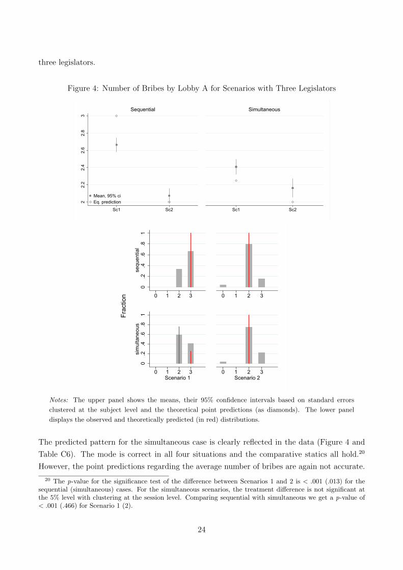
Notes: The upper panel shows the means, their 95% confidence intervals based on standard errors

clustered at the subject level and the theoretical point predictions (as diamonds). The lower panel

displays the observed and theoretically predicted (in red) distributions.

The predicted pattern for the simultaneous case is clearly reflected in the data (Figure 4 and

Table C6). The mode is correct in all four situations and the comparative statics all hold.20

However, the point predictions regarding the average number of bribes are again not accurate.

20 The p-value for the significance test of the difference between Scenarios 1 and 2 is < .001 (.013) for thesequential (simultaneous) cases. For the simultaneous scenarios, the treatment difference is not significant atthe 5% level with clustering at the session level. Comparing sequential with simultaneous we get a p-value of< .001 (.466) for Scenario 1 (2).

24

Table 6: Results for Scenarios with Three Legislators

Sc1 se Sc2 se

# Bribes proposed by A:Equilibrium: sequential 3 2Observed: sequential 2.66 (0.04) 2.07 (0.05)Equilibrium: simultaneous 2.25 2Observed: simultaneous 2.41 (0.04) 2.16 (0.06)

# Bribes proposed by B:Equilibrium: sequential 0 0Observed: sequential 0.4 (0.06) 0.31 (0.05)Observed: simultaneous 0.72 (0.1) 0.97 (0.09)

Votes won by A:Observed: sequential 2.35 (0.06) 1.77 (0.07)Observed: simultaneous 2.27 (0.06) 1.84 (0.07)

A wins (%):Equilibrium: sequential 100 100Observed: sequential 83.17 (3.12) 73.68 (3.96)Equilibrium: simultaneous <100 <100Observed: simultaneous 92.86 (2.53) 79.59 (3.9)

Total bribes proposed by A:Equilibrium: sequential 5 14Observed: sequential 6.54 (0.25) 11.92 (0.44)Equilibrium: simultaneous 2.25 11Observed: simultaneous 6.66 (0.33) 11.66 (0.44)

Total bribes proposed by B:Equilibrium: sequential 0 0Observed: sequential 0.7 (0.13) 0.46 (0.08)Observed: simultaneous 0.83 (0.21) 1.26 (0.24)

Winning coalition size if A wins:Observed: sequential 2.64 (0.04) 2.14 (0.04)Observed: simultaneous 2.38 (0.04) 2.18 (0.04)

Winning coalition size if B wins:Observed: sequential 2.12 (0.05) 2.28 (0.07)Observed: simultaneous 2.29 (0.1) 2.5 (0.1)

Levelling by A (%):Equilibrium: sequential 100 100Observed: sequential 86.9 (4.56) 95.71 (3.12)Equilibrium: simultaneous 100 0-100Observed: simultaneous 87.91 (4.66) 87.18 (4.82)

Notes: Standard errors (ses) are clustered at the subject level.The theoretical predictions for the simultaneous case are expectedvalues.

25

The same holds for the total sum of bribes offered (Table 6 and Table C7). We observe

again that Lobby A wins more often in the simultaneous-moves case, which goes against the

theoretical predictions.21 Most Lobby B’s number of offered bribes are again close to zero in

the sequential scenarios (Figures C7 and C9) but their means are again strongly significantly

larger than zero.

3.2.2 Leveling

Leveling is very prevalent in both sub-treatments and both scenarios: at least 86% of the

Lobbies A adopt a leveling strategy. However, this is not very surprising as the number of

strategies that are not leveling and not weakly dominated is much lower as a result of the

much lower willingness to pay compared to the seven-legislators scenarios. The differences in

the distributions of bribes for each legislator again indicate different strategy choices in the

sequential as compared to the simultaneous treatments (Figures C8 and C9).

3.2.3 Errors, Learning, and Heterogeneity

Figure 5: Lobbies A’s Deviations from Equilibrium and Payoffs

-20

-10

010

Payo

ff

-15 -10 -5 0 5 10

Deviation

Lowess Smoother

Sequential

-20

-10

010

Payo

ff

-10 0 10 20 30

Deviation

Lowess Smoother

Simultaneous

Note: Scatter plots and lowess smoothers of Lobbies A’s deviations from theoretically predicted total

sum of bribes and Lobbies A’s normalized payoffs. Payoffs are normalized by de-meaning them by

scenario. To avoid overlay a random jitter was used.

21The difference is only significant when the two scenarios are pooled.

26

Figure 5 shows Lobbies A’s payoffs and deviations from the theoretically predicted total sum

of offered bribes. As in the seven-legislator scenarios, the lowess smoother peaks close to zero

both under sequential and simultaneous moves, suggesting that bidding the predicted optimal

amount (or again slightly more) is optimal. Regressions of Lobby A’s payoffs on deviations

from the theoretically predicted total sum of offered bribes, or on the deviations from the

theoretically predicted number of bribes, lend further evidence on the costs of deviating much

from equilibrium (Table C8). There is less learning than in the seven legislator scenarios and

we only see a significant decline in the errors over time for deviations from the theoretically

predicted total sum of bribes under simultaneous moves (Table C9).

Regarding heterogeneity of subjects, we focus again on subjects who played in the role of

Lobby A in at least three rounds (96% of all subjects). We observe that exactly one subject

plays the theoretically predicted strategy exactly in all rounds with sequential scenarios, and

17% play it in 50% or more of the rounds. Moreover, 67% (67%) of the subjects always play

a leveling strategy in both sequential (simultaneous) scenarios. Looking again for subjects

playing strategies far from the theoretical predictions, we see that 35% (35%) of the subjects

who played in the role of Lobby A in at least three rounds are at or above the 75th percentile

of the distributions of the deviations from theoretically predicted total sum of offered bribes in

more than half of the sequential (simultaneous) rounds they play.22 Deviating at or above this

percentile leads to a payoff that is, on average, 2.4 (1.8) points lower than that of the other

Lobbies A in the sequential (simultaneous) rounds. Turning to subjects who frequently play

strategies that are relatively close to the theoretical predictions, we see that 42% (34%) of the

subjects are at or below the 25th percentile of the distributions of the deviations in more than

than half of the sequential (simultaneous) scenarios they played. Being in this group gives them

a payoff that is, on average, 3.9 (1.6) points higher than that of the rest.

3.3 Summary of Key Results

Following the predictions as stated in Section 2, we summarize the main empirical findings for

the sequential scenarios as follows:

1. There are no scenarios in which both lobbies make payments. While it is true

that Lobbies B bid close to zero, on average, in all seven scenarios, Lobbies A’s deviation

from the theoretical predictions and the apparent willingness of some Lobbies B to incur

a (small) loss for winning, leads to average bid levels that are slightly (but significantly)

higher than zero in all scenarios (see Tables 5 and 6).

2. The first-mover lobby will use a leveling strategy. Indeed, leveling strategies are

22Note that many subjects offer the same total sum of bribes in the three legislator scenarios. Hence, morethan 25% can be at or below the 25th percentile of the distribution.

27

very prevalent. However, the frequency declines for Scenarios 6 and 7, suggesting that

a substantial number of subjects did not entirely understand the rationale of leaving no

soft spots (see Tables 5 and 6).

3. The optimal sizes of the majorities (weakly) decrease in the legislators’ biases

in favor of the status quo and (weakly) increases with the prize for B. The

comparative statics predictions resulting from these predictions all hold except for the

comparison between Scenario 2 and 4 (see Table 4), where the average number of bribes

in Scenario 4 is lower than expected because of one third of Lobbies A bidding zero (see

Figure 1).

4. Either Lobby A will win the vote for sure (if WA ≥ CA), or Lobby B will win

for sure (if WA < CA). We observe that the lobby that is predicted to win does so with

high probability albeit with a probability substantially below 100%. Exceptions are the

two scenarios 4 and 7 where A is predicted to win for sure but B wins frequently. These

are the two scenarios in which it is most expensive for A to win (see Tables 5 and 6).

Regarding the predictions for the simultaneous scenarios, we find the following:

1. Both lobbies will make positive payment offers. This is supported in the data for

all scenarios (see Tables 5 and 6).

2. The frequency of leveling strategies will be lower in the simultaneous relative

to the sequential game set-up. This is supported in the data.

3. The optimal sizes of the majorities (weakly) decrease in the legislators’ biases

in favor of the status quo and (weakly) increases with the prize for B. Most of

the comparative statics predictions resulting from these predictions do indeed hold in the

data but several treatment differences are not significant (see Table C1).

4. The winning probability of A will be lower in the simultaneous game than in

the sequential legislative lobbying game. This hypothesis has not found support in

the data (see Tables 5 and 6).

While not all hypotheses are supported in the data, subjects’ behavior mostly responds to the

incentives in the predicted direction in both the simultaneous and sequential treatments. As a

result, supermajorities are often formed and majority size varies with Lobby B’s willingness to

pay and the voters’ valuations. In an overall mixed picture, the central insights of Groseclose

and Snyder (1996) thus appear valid.

28

4 Conclusions

We set out to test the key predictions of the seminal vote-buying model by Groseclose and

Snyder (1996). We design nine different scenarios, varying the number of legislators (three and

seven) between sessions, and the relative willingness to pay of the lobbies and the preference

biases of the legislators within sessions. To the best of our knowledge, this is the first experi-

mental study of this model. A key feature of our experiment is that we run treatments with the

sequential-moves structure, as assumed in the original model, as well as treatments in which

this assumption is relaxed and the subjects move simultaneously instead. We argue, and show

theoretically for the three-legislators scenarios, that the key comparative statics predictions of

the GS model carry over to the simultaneous-moves case.

In the experiment, we find for the sequential-moves set-up that most comparative statics

predictions are borne out by the data. The main insights regarding how the majority size

depends on the relative willingness to pay of the lobbies and on the biases of the legislators are

confirmed. However, other, more specific predictions regarding the exact number and level of

bribes are inaccurate. Turning to the simultaneous set-up, we find that the main comparative

statics predictions still hold but that behavior varies much more and the predictive power of

the sequential-moves model is reduced substantially. Overall, this suggests that the GS model

does capture some important insights that are even robust to the relaxation of the central

modeling assumption of sequential moves. However, its predictive power is substantially lower

when the sequentiality assumption is relaxed, and it is also limited with respect to the more

specific predictions regarding individual strategies in the sequential-moves treatments.

In stress-testing a seminal model by relaxing a central model assumption our paper shares

similarities with the work of Tremewan and Vanberg (2016), who study legislative bargaining in

an arguably more realistic but not theoretically (analytically) solvable set-up than that in the

established bargaining models. We see this approach, which is much less often followed than

simply implementing the original structure of a game theoretic model, as a useful complement.

It allows for new insights into how strongly predictions depend on certain modeling assumptions

which might not hold in the field, and thus speaks to external validity concerns regarding a

model’s predictions. We believe that more studies of this kind would be highly valuable.

29

References

Arad, A. and Rubinstein, A. (2012). Multi-dimensional iterative reasoning in action: The case

of the Colonel Blotto game. Journal of Economic Behavior & Organization, 84(2):571–585.

Banks, J. (2000). Buying supermajorities in finite legislatures. American Political Science

Review, 94(3):677–681.

Bernheim, B. D. and Whinston, M. D. (1986). Menu Auctions, Resource Allocation, and

Economic Influence. The Quarterly Journal of Economics, 101(1):1.

Borel, E. (1921). La theorie du jeu les equations integrales a noyau symetrique. Comptes

Rendus de l’Academie, 173:1304–8.

Casella, A., Laslier, J. F., and Mace, A. (2017). Democracy for Polarized Committees. The

Tale of Blotto’s Lieutenants. Games and Economic Behavior, 106:239–259.

Chowdhury, S. and Kovenock, D. (2013). An experimental investigation of Colonel Blotto

games. Economic Theory, 52(3):833–861.

Crawford, V. and Sobel, J. (1982). Strategic information transmission. Econometrica,

50(6):1431–1451.

Dechenaux, E., Kovenock, D., and Sheremeta, R. M. (2015). A survey of experimental research

on contests, all-pay auctions and tournaments. Experimental Economics.

Dekel, E., Jackson, M., and Wolinsky, A. (2008). Vote Buying: General Elections. Journal of

Political Economy, 116(2):351–380.

Dekel, E., Jackson, M. O., and Wolinsky, A. (2009). Vote Buying: Legislatures and Lobbying.

Quarterly Journal of Political Science, 4(2):103–128.

Diermeier, D. and Myerson, R. (1999). Bicameralism and its Consequences for the Internal

Organization of Legislatures. American Economic Review, 89(5):1182–1196.

Ellis, C. J. and Groll, T. (2017). Strategic Legislative Subsidies: Informational Lobbying and

the Cost of Policy. Mimeo.

Fischbacher, U. (2007). Z-Tree: Zurich toolbox for ready-made economic experiments. Experi-

mental Economics, 10(2):171–178.

Groseclose, T. and Snyder, J. (1996). Buying supermajorities. American Political Science

Review, 90(2):303–315.

30

Grossman, G. and Helpman, E. (1994). Protection for sale. The American Economic Review,

84(4):833–850.

Grossman, G. and Helpman, E. (2001). Special Interest Politics. The MIT Press, Cambridge,

MA.

Hall, R. L. and Deardorff, A. V. (2006). Lobbying as Legislative Subsidy. American Political

Science Review, 100(01):69–84.

Hortala-Vallve, R. and Llorente-Saguer, A. (2012). Pure strategy Nash equilibria in non-zero

sum colonel Blotto games. International Journal of Game Theory, 41:331–343.

Hortala-Vallve, R. and Llorente-Saguer, A. (2015). An Experiment on Non-Zero Sum Colonel

Blotto Games. Mimeo.

Hummel, P. (2009). Buying supermajorities in a stochastic environment. Public Choice, (De-

cember 2008):351–369.

Kirchsteiger, G. and Prat, A. (2001). Inefficient equilibria in lobbying. Journal of Public

Economics, 82(3):349–375.

Konrad, K. A. and Kovenock, D. (2009). Multi-battle contests. Games and Economic Behavior,

66(1):256–274.

Kovenock, D. and Roberson, B. (2012). Conflicts with multiple battlefields. In The Oxford

Handbook of the Economics of Peace and Conflict, pages 503–531.

Kvasov, D. (2007). Contests with limited resources. Journal of Economic Theory, 136(1):738–

748.

Le Breton, M. and Zaporozhets, V. (2010). Sequential Legislative Lobbying under Political

Certainty. The Economic Journal, 120(543):281–312.

Mago, S. D. and Sheremeta, R. M. (2017). Multi-battle Contests: An Experimental Study.

Southern Economic Journal, 84(2):407–425.

McKelvey, R. D., McLennan, A. M., and Turocy, T. L. (2016). Gambit: Software tools for

game theory, version 16.0.1.

Montero, M., Possajennikov, A., Sefton, M., and Turocy, T. L. (2016). Majoritarian Blotto

Contests with Asymmetric Battlefields: An Experiment on Apex Games. Economic Theory,

61(1):55–89.

31

Morton, R. B. and Williams, K. C. (2010). Experimental Political Science and the Study of

Causality: From Nature to the Lab. Cambridge University Press.

Roberson, B. (2006). The Colonel Blotto game. Economic Theory, 29:1–24.

Roberson, B. and Kvasov, D. (2012). The non-constant-sum Colonel Blotto game. Economic

Theory, 51(2):397–433.

Schneider, M. T. (2014). Interest-group size and legislative lobbying. Journal of Economic

Behavior and Organization, 106:29–41.

Schneider, M. T. (2017). Who Writes the Bill? The Role of the Agenda-Setter in Legislative

Lobbying. Mimeo.

Szentes, B. and Rosenthal, R. W. (2003a). Beyond chopsticks: Symmetric equilibria in majority

auction games. Games and Economic Behavior, 45(2):278–295.

Szentes, B. and Rosenthal, R. W. (2003b). Three-object two-bidder simultaneous auctions:

Chopsticks and tetrahedra. Games and Economic Behavior, 44(1):114–133.

Tremewan, J. and Vanberg, C. (2016). The dynamics of coalition formation – A multilat-

eral bargaining experiment with free timing of moves. Journal of Economic Behavior and

Organization, 130:33–46.

32

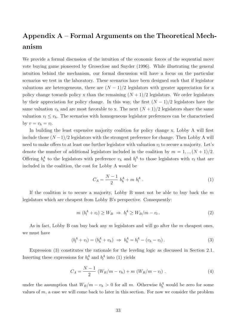
Appendix A – Formal Arguments on the Theoretical Mech-

anism

We provide a formal discussion of the intuition of the economic forces of the sequential move

vote buying game pioneered by Groseclose and Snyder (1996). While illustrating the general

intuition behind the mechanism, our formal discussion will have a focus on the particular

scenarios we test in the laboratory. These scenarios have been designed such that if legislator

valuations are heterogeneous, there are (N − 1)/2 legislators with greater appreciation for a

policy change towards policy x than the remaining (N + 1)/2 legislators. We order legislators

by their appreciation for policy change. In this way, the first (N − 1)/2 legislators have the

same valuation vh and are most favorable to x. The next (N + 1)/2 legislators share the same

valuation vl ≤ vh. The scenarios with homogeneous legislator preferences can be characterised

by v = vh = vl.

In building the least expensive majority coalition for policy change x, Lobby A will first

include those (N−1)/2 legislators with the strongest preference for change. Then Lobby A will

need to make offers to at least one further legislator with valuation vl to secure a majority. Let’s

denote the number of additional legislators included in the coalition by m = 1, .., (N + 1)/2.

Offering bAh to the legislators with preference vh and bAl to those legislators with vl that are

included in the coalition, the cost for Lobby A would be

CA =N − 1

2bAh + m bAl . (1)

If the coalition is to secure a majority, Lobby B must not be able to buy back the m

legislators which are cheapest from Lobby B’s perspective. Consequently:

m (bAl + vl) ≥ WB ⇒ bAl ≥ WB/m− vl . (2)

As in fact, Lobby B can buy back any m legislators and will go after the m cheapest ones,

we must have

(bAl + vl) = (bAh + vh) ⇒ bAh = bAl − (vh − vl) . (3)

Expression (3) constitutes the rationale for the leveling logic as discussed in Section 2.1.

Inserting these expressions for bAh and bAl into (1) yields

CA =N − 1

2(WB/m− vh) + m (WB/m− vl) . (4)

under the assumption that WB/m − vh > 0 for all m. Otherwise bAh would be zero for some

values of m, a case we will come back to later in this section. For now we consider the problem

33

of Lobby A of chosing the optimal m to minimise CA under the given assumption.

Taking the derivative of CA with respect to m gives

dCA

dm= −vl −

N − 1

2

WB

m2. (5)

This illustrates the two forces at play when choosing the optimal coalition size: If the

legislators preferences vl are negative, that is opposed to the policy change, any further legislator

in the coalition must be compensated for that. This makes a larger coalition more expensive.

However, with a larger coalition, Lobby B needs to buy back more legislators. This allows

to reduce the amount of payments offered to each legislator. In particular, as Lobby B only

needs to buy back m legislators of the coalition, a larger coalition size allows Lobby A to save

on bribes for the additional (N − 1)/2 legislators they need to make payments to. This effect

makes a larger coalition less expensive. We observe in (5) that the costs of the coalition CA are

monotonically declining in coalition size if vl ≥ 0. With vl negative, there is a trade-off and the

optimal size can be calculated as23

m∗ =

√WB(N − 1)

−2 vl. (6)

Expression 6 reflects the discussion in showing that the optimal coalition size declines with

the legislators preference intensity for the status quo −vl and increases with the willingness to

pay for Lobby B.

We can now relate our lab scenarios to this discussion. As shown in Table 1, legislators have

homogeneous preferences in the first five scenarios. Scenarios 1-4 illustrate the effects of the

legislators’ preferences and Lobby B’s willingness to pay on the optimal sizes of the coalitions

formed by Lobby A.

In Scenario 1, the legislators have no preferences (except the tie breaking -0.5) for any

of the two policy options. In accordance with (5), the cost of the coalition of A is strictly

declining in coalition size and including all legislators will be optimal. Hence, m = 4 and

the optimal coalition size is N = 7. Comparing Scenario 1 with Scenario 2 illustrates how a

stronger preference of the legislators (−19.5) against the policy change favored by Lobby A

makes maintaining large coalition sizes much more expensive as illstrated in expressions (5)

and (6). As a consequence the optimal size reduces to a simple majority of 4 in Scenario 2.

However, when comparing Scenario 2 to Scenario 4, the optimal coalition size increases to 6.

The only dfference between these to scenarios is the substiantially higher willingness to pay

by Lobby B, WB, which leads to higher marginal reductions in costs of larger coalitions as

23Note that in order to derive the optimal coalition sizes in our lab scenarios, m∗ needs to be rounded up tothe next integer.

34

reflected in (5). Scenarios 1-4 also illustrate that the cost reducing effect of larger coalition size

is stronger when Lobby B’s prize is larger in the following way: In response to higher status

quo bias of the legislators, the reduction in optimal coalition size (by 3) is larger when WB = 12

as observed in the comparison between Scenarios 1 and 3 than the reduction in coalition size

(by 1) when WB = 60 observed when comparing scenarios 2 and 4.

Scenario 5 captures the situation where the prize for Lobby B is so high that the costs of

any majority coalition will be much larger than Lobby A’s willingness to pay. In this example,

CA = 455 > 200 = WA. Therefore it is optimal for Lobby A to abstain from making positive

payment offers.

Scenarios 6 and 7 feature heterogeneous preferences by legislators where 3 of the legislators

are in favor of policy change while 4 possess a strong preference for the status quo. Our previous

general discussion applies to Scenario 7 where expression (5) reveals that the marginal effects

are the same as in Scenario 4 because the preferences of the (N + 1)/2 legislators most opposed

to policy change as well as WB are the same. Therefore the optimal size of the coalition is 6.

In particular, the optimal strategy is to offer a payment of 40 to 3 legislators opposed to policy

change and to offer 8 to one and 7 to the other two legislators in favor of policy change.24 In

this way, the condition WB/m − vh > 0, i.e. 60/3 − 12.5 = 7.5 > 0 holds and it is optimal

for Lobby A to make positive payments to all legislators in the coalition, i.e. build a flooded

coalition.

This is different in Scenario 6, where WB = 12 and hence WB < vh. This implies that Lobby

B’s willingness to pay is not high enough to make a pro-change legislator vote for the status

quo. The condition WB/m − vh > 0 will not hold for any m in this scenario. Therefore, it is

not necessary for Lobby A to make any payments to the legislators in favor of policy change. It

is optimal for Lobby A to form a non-flooded coalition. As a consequence, however, the benefit

when increasing coalition size of being able to reduce the payments to the (N − 1)/2 legislators

that need not be bought back by Lobby B, as captured by the last summand in expression (5),

disappears. When increasing coalition size, Lobby A is then left with only the cost increasing

effect of compensating the legislators least favorable to policy change. Hence it is cheapest to

form the smallest possible majority coalition of 4.

24Note that the reason for not offering the same amount to all legislators favoring policy change is due toallowing only integer payments as discussed in Section 2.1.

35

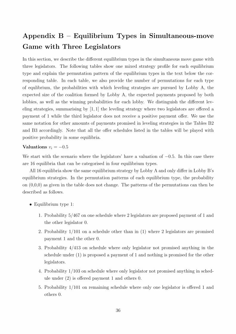
Appendix B – Equilibrium Types in Simultaneous-move

Game with Three Legislators

In this section, we describe the different equilibrium types in the simultaneous move game with

three legislators. The following tables show one mixed strategy profile for each equilibrium

type and explain the permutation pattern of the equilibrium types in the text below the cor-

responding table. In each table, we also provide the number of permutations for each type

of equlibrium, the probabilities with which leveling strategies are pursued by Lobby A, the

expected size of the coalition formed by Lobby A, the expected payments proposed by both

lobbies, as well as the winning probabilities for each lobby. We distinguish the different lev-

eling strategies, summarising by [1, 1] the leveling strategy where two legislators are offered a

payment of 1 while the third legislator does not receive a positive payment offer. We use the

same notation for other amounts of payments promised in leveling strategies in the Tables B2

and B3 accordingly. Note that all the offer schedules listed in the tables will be played with

positive probability in some equilibria.

Valuations vi = −0.5

We start with the scenario where the legislators’ have a valuation of −0.5. In this case there

are 16 equilibria that can be categorised in four equilibrium types.

All 16 equilibria show the same equilibrium strategy by Lobby A and only differ in Lobby B’s

equilibrium strategies. In the permutation patterns of each equilibrium type, the probability

on (0,0,0) as given in the table does not change. The patterns of the permutations can then be

described as follows.

• Equilibrium type 1:

1. Probability 5/467 on one schedule where 2 legislators are proposed payment of 1 and

the other legislator 0.

2. Probability 1/101 on a schedule other than in (1) where 2 legislators are promised

payment 1 and the other 0.

3. Probability 4/413 on schedule where only legislator not promised anything in the

schedule under (1) is proposed a payment of 1 and nothing is promised for the other

legislators.

4. Probability 1/103 on schedule where only legislator not promised anything in sched-

ule under (2) is offered payment 1 and others 0.

5. Probability 1/101 on remaining schedule where only one legislator is offered 1 and

others 0.

36

Table B1: Equilibrium Types for Scenarios with Simulteneous Moves and Three Legislatorswith Valuation vi = −0.5

Equilibrium Type

Schedule 1 2 3 4

Lobby A (0,1,1) 1/4 1/4 1/4 1/4(1,0,1) 1/4 1/4 1/4 1/4(1,1,0) 1/4 1/4 1/4 1/4(1,1,1) 1/4 1/4 1/4 1/4

Lobby B (0,0,0) 495/521 24/25 131/138 98/101(0,0,1) 4/413 5/516 4/413 1/101(0,1,0) 1/101 1/101 8/809 1/101(1,0,0) 1/103 1/101 1/103 1/101(0,1,1) 1/101 0 8/809 0(1,0,1) 0 0 0 0(1,1,0) 5/467 5/476 4/373 0

Permuations 6 3 6 1Prob. Levelling A, [1, 1] 3/4 3/4 3/4 3/4Prob. Levelling A, (1, 1, 1) 1/4 1/4 1/4 1/4Total Prob. Levelling A 1 1 1 1Exp. Coalition size A 2.25Exp. Bribes proposed by A 2.25Exp. Payments by A 2.19 2.21 2.19 2.23Exp. Bribes proposed by B 0.07 0.05 0.07 0.03Exp. Payments by B 0.06 0.04 0.06 0.02Winning prob. A 0.96 0.97 0.96 0.99Winning prob. B 0.04 0.03 0.04 0.01

37

There are 6 permutations of equilibrium type 1.

• Equilibrium type 2:

1. Probability 5/476 on one schedule where 2 legislators are promised payment of 1 and

remaining legislator is offered nothing.

2. Probability 5/516 on schedule where only legislator not promised anything in sched-

ule under (1) is offered payment 1 and others 0.

3. Probability 1/101 on the two schedules other than in (2) where only one legislator

is offered a payment of 1 and the others 0.

There are 3 permutations of equilibrium type 2.

• Equilibrium type 3:

1. Probability 4/373 on one schedule where 2 legislators are promised a payment of 1

and other legislator nothing.

2. Probability 8/809 on a schedule other than in (1) where 2 legislators are offered

payment 1 and other legislator 0.

3. Probability 4/413 on schedule where only legislator not offered anything in schedule

under (1) obtains payment 1 and others nothing.

4. Probability 1/103 on schedule where only legislator not promised anything in sched-

ule under (2) is offered payment 1 and others nothing.

5. Probability 8/809 on remaining schedule where only one legislator is proposed 1 and

others 0.

There are 6 permutations of equilibrium type 3.

• Equilibrium type 4: The only permutation is shown in the table.

Valuations vi = −4.5, Equilibrium types 1-6

We now turn to the scenario where legislators have valuation −4.5. There are 56 equilibria

which can be summarised in 12 equilibrium types. We first describe the patterns of the first 6

equilibrium types and will discuss the patterns of the remaining 6 equilibrium types below.

All of these 6 equilibrium types show the same permutation patterns of Lobby A’s equilib-

rium strategies: One legislator is offered a payment of 6 with certainty and the two remaining

legislators will receive a payment of 5 or 0 with probability 1/2. The permutation patterns by

Lobby B in each equilibrium type can be described as follows.

• Equilibrium type 1:

38

Table B2: Equilibrium Types for Scenarios with Simulteneous Moves and Three Legislatorswith Valuation vi = −4.5

Equilibrium Type

Schedule 1 2 3 4 5 6

Lobby A (0,5,6) 1/2 1/2 1/2 1/2 1/2 1/2(0,6,5) 0 0 0 0 0 0(5,0,6) 1/2 1/2 1/2 1/2 1/2 1/2(5,6,0) 0 0 0 0 0 0(6,0,5) 0 0 0 0 0 0(6,5,0) 0 0 0 0 0 0

Lobby B (0,0,0) 0 2/5 377/405 14/15 386/405 1/5(0,0,1) 43/45 5/9 2/81 1/45 1/405 34/45(0,1,0) 0 1/45 1/45 1/45 0 0(1,0,0) 0 1/45 0 1/45 0 1/45(0,1,1) 1/45 0 0 0 1/45 1/45(1,0,1) 1/45 0 1/45 0 1/45 0(1,1,0) 0 0 0 0 0 0

Permuations 3 3 6 3 3 6Prob. Levelling A, [6, 6] 0 0 0 0 0 0Prob. Levelling A, [5, 5] 0 0 0 0 0 0Total Prob. Levelling A 0 0 0 0 0 0Exp. Coalition size A 2Exp. Bribes proposed by A 11Exp. Payments by A 10.978Exp. Bribes proposed by B 1.044 0.6 0.091 0.067 0.091 0.822Exp. Payments by B 0.044Winning prob. A 0.978Winning prob. B 0.022

39

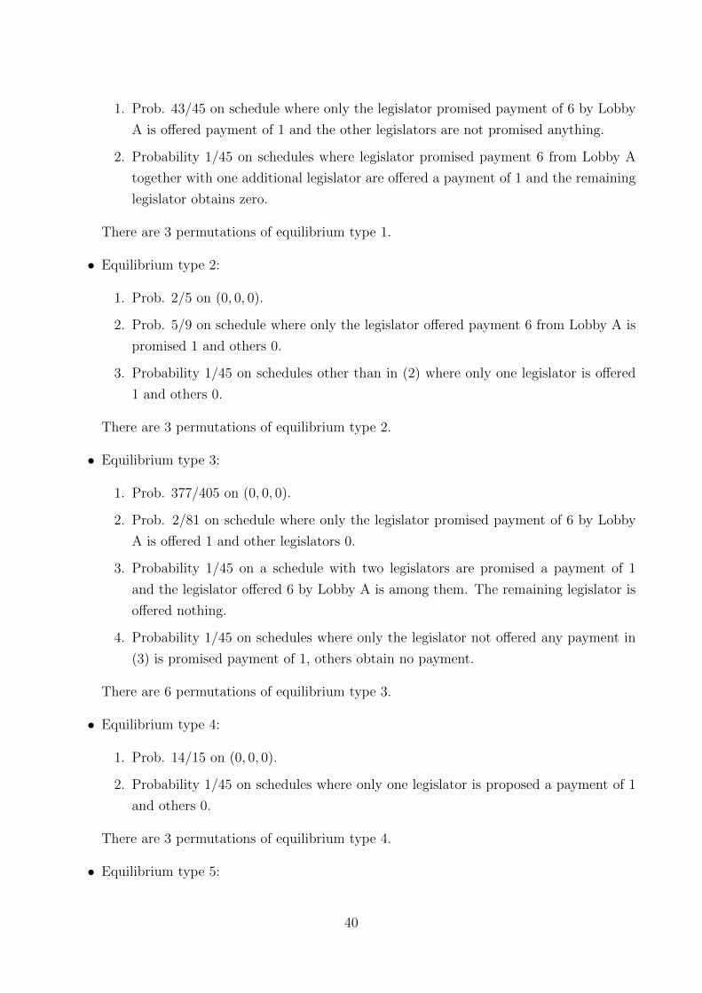
1. Prob. 43/45 on schedule where only the legislator promised payment of 6 by Lobby

A is offered payment of 1 and the other legislators are not promised anything.

2. Probability 1/45 on schedules where legislator promised payment 6 from Lobby A

together with one additional legislator are offered a payment of 1 and the remaining

legislator obtains zero.

There are 3 permutations of equilibrium type 1.

• Equilibrium type 2:

1. Prob. 2/5 on (0, 0, 0).

2. Prob. 5/9 on schedule where only the legislator offered payment 6 from Lobby A is

promised 1 and others 0.

3. Probability 1/45 on schedules other than in (2) where only one legislator is offered

1 and others 0.

There are 3 permutations of equilibrium type 2.

• Equilibrium type 3:

1. Prob. 377/405 on (0, 0, 0).

2. Prob. 2/81 on schedule where only the legislator promised payment of 6 by Lobby

A is offered 1 and other legislators 0.

3. Probability 1/45 on a schedule with two legislators are promised a payment of 1

and the legislator offered 6 by Lobby A is among them. The remaining legislator is

offered nothing.

4. Probability 1/45 on schedules where only the legislator not offered any payment in

(3) is promised payment of 1, others obtain no payment.

There are 6 permutations of equilibrium type 3.

• Equilibrium type 4:

1. Prob. 14/15 on (0, 0, 0).

2. Probability 1/45 on schedules where only one legislator is proposed a payment of 1

and others 0.

There are 3 permutations of equilibrium type 4.

• Equilibrium type 5:

40

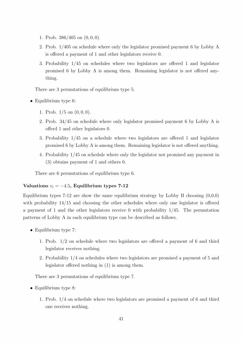
1. Prob. 386/405 on (0, 0, 0).

2. Prob. 1/405 on schedule where only the legislator promised payment 6 by Lobby A

is offered a payment of 1 and other legislators receive 0.

3. Probability 1/45 on schedules where two legislators are offered 1 and legislator

promised 6 by Lobby A is among them. Remaining legislator is not offered any-

thing.

There are 3 permutations of equilibrium type 5.

• Equilibrium type 6:

1. Prob. 1/5 on (0, 0, 0).

2. Prob. 34/45 on schedule where only legislator promised payment 6 by Lobby A is

offerd 1 and other legislators 0.

3. Probability 1/45 on a schedule where two legislators are offered 1 and legislator

promised 6 by Lobby A is among them. Remaining legislator is not offered anything.

4. Probability 1/45 on schedule where only the legislator not promised any payment in

(3) obtains payment of 1 and others 0.

There are 6 permutations of equilibrium type 6.

Valuations vi = −4.5, Equilibrium types 7-12

Equilibrium types 7-12 are show the same equilibrium strategy by Lobby B choosing (0,0,0)

with probability 14/15 and choosing the other schedules where only one legislator is offered

a payment of 1 and the other legislators receive 0 with probability 1/45. The permutation

patterns of Lobby A in each equilibrium type can be described as follows.

• Equilibrium type 7:

1. Prob. 1/2 on schedule where two legislators are offered a payment of 6 and third

legislator receives nothing.

2. Probability 1/4 on schedules where two legislators are promised a payment of 5 and

legislator offered nothing in (1) is among them.

There are 3 permutations of equilibrium type 7.

• Equilibrium type 8:

1. Prob. 1/4 on schedule where two legislators are promised a payment of 6 and third

one receives nothing.

41

Table B3: Equilibrium Types for Scenarios with Simulteneous Moves and Three Legislatorswith Valuation −4.5

Equilibrium Type

Schedule 7 8 9 10 11 12

Lobby A (0,5,5) 1/4 1/4 0 1/3 1/6 1/5(5,0,5) 1/4 0 0 0 0 0(5,5,0) 0 0 0 0 1/6 0(5,5,5) 0 0 0 0 0 0(0,5,6) 0 0 1/3 0 0 0(0,6,5) 0 0 0 0 0 0(5,0,6) 0 1/4 0 0 1/3 2/5(5,6,0) 0 1/4 1/3 1/3 0 0(6,0,5) 0 0 1/3 0 0 0(6,5,0) 0 0 0 0 0 1/5(0,6,6) 0 1/4 0 0 1/3 1/5(6,0,6) 0 0 0 1/3 0 0(6,6,0) 1/2 0 0 0 0 0

Lobby B (0,0,0) 14/15 14/15 14/15 14/15 14/15 14/15(0,0,1) 1/45 1/45 1/45 1/45 1/45 1/45(0,1,0) 1/45 1/45 1/45 1/45 1/45 1/45(1,0,0) 1/45 1/45 1/45 1/45 1/45 1/45

Permuations 3 9 2 6 6 6Prob. Levelling A, [6, 6] 1/2 1/4 0 1/3 1/3 1/5Prob. Levelling A, [5, 5] 1/2 1/4 0 1/3 1/3 1/5Total Prob. Levelling A 1 1/2 0 2/3 2/3 2/5Exp. Coalition size A 2Exp. Bribes proposed by A 11Exp. Payments by A 10.978Exp. Bribes proposed by B 0.067Exp. Payments by B 0.044Winning prob. A 0.978Winning prob. B 0.022

42

2. Prob. 1/4 on schedule where two legislators are offered a payment of 5 and remaining

legislator receives nothing.

3. Probability 1/4 on those two schedules with payments 6,5 and 0 such that overall

one legislator is offered payment 5 with prob. 1/4 and zero otherwise and the other

two legislators are each proposed a payment of 6 with prob. 1/2 and a payment of

5 with prob. 1/4.

There are 9 permutations of equilibrium type 8.

• Equilibrium type 9:

1. Probability 1/3 on three schedules with payments 6,5 and 0 such that overall each

legislator is offered payments 6, 5 and 0 with prob. 1/3.

There are 2 permutations of equilibrium type 9.

• Equilibrium type 10:

1. Probability 1/3 on one schedule where two legislators are promised 6 and the re-

maining legislator is offered nothing.

2. Probability 1/3 on one schedule where two legislators are offered 5 and the remaining

legislator nothing and the legislator receiving nothing in (1) is among the two offered

5.

3. Probability 1/3 on those schedules with payments 6,5 and 0 such that overall each

legislator is offered payments 6, 5 and 0 with prob. 1/3.

There are 6 permutations of equilibrium type 10.

• Equilibrium type 11:

1. Probability 1/6 on two schedules where two legislators are promised 5 and the other

legislator obtains 0.

2. Probability 1/3 on one schedule where two legislators are offered 6 and third legislator

nothing and probability 1/3 on a schedule with payments 6,5 and 0 in such a way

that overall one legislator is offered payments 6, 5 and 0 with probabilies 2/3, 1/6

and 1/6, one with probabilities 1/3, 1/3 and 1/3 and one with 0, 1/2 and 1/2.

There are 6 permutations of equilibrium type 11.

• Equilibrium type 12:

43

1. Probability 1/5 on one schedule where two legislators are promised 6 and the re-

maining legislator obtains 0.

2. Probability 1/5 on one schedule where the same two legislators as in (1) are offered

a payment of 5 and the remaining legislator receives nothing.

3. Probability 2/5 on a schedule with payments 6,5 and 0 where legislator offered

nothing in (1) and (2) is proposed payment of 5.

4. Probability 1/5 on a schedule with payments 6,5 and 0 where legislator receiving

nothing in (1) and (2) is offered a payment of 6 and legislator receiving nothing in

(3) is offered 5.

There are 6 permutations of equilibrium type 12.

44

Appendix C – Additional Tables and Figures

Table C1: Comparative Statics 7 Legislators Simultaneous: Number of Bribes of Lobby A

Sc.1 Sc.2 Sc.3 Sc.4 Sc.5 Sc.6 Sc.7

Sc.1 > > > > > > >p-value .338 .001 .76 .002† .001† .000† .000†

Sc.2 > < < > > <p-value .941 .001 .505 .213 .336 .649

Sc.3 > > > > >p-value .008 .005 .001† .000 .000

Sc.4 < > > >p-value .018† .130 .207 .382

Sc.5 > < <p-value .000 .613 .311

Sc.6 < <p-value .000 .609

Sc.7 >p-value .290

Notes: > (<): average number of bribes in row scenario greater (smaller)

than column scenario; in the diagonal the scenario with simultaneous moves

is tested against the same scenario with sequential moves; all off-diagonal

comparisons are between simultaneous-moves scenarios; p-value are for two-

sided tests. †: significant at 5% with clustering at subject level but not with

clustering at session level.

45

Table C2: Number of Bribes of Lobby A – Seven Legislators

1–5 seq 1–5 sim 6–7 seq 6–7 sim All seq All sim

GS prediction 0.67*** 0.19*** 0.53*** 0.03 0.62*** 0.16***(0.05) (0.05) (0.08) (0.06) (0.05) (0.04)

cons 1.01*** 4.27*** 1.96*** 4.57*** 1.37*** 4.33***(0.27) (0.31) (0.35) (0.31) (0.22) (0.24)

N 205 200 82 80 287 280R2 0.42 0.10 0.35 0.00 0.40 0.07N clust 80 77 62 58 80 80

Notes: * p < 0.10, ** p < 0.05, *** p < 0.01. Standard errors in parentheses are

clustered at the subject level. The first two column refer to Scenarios 1–5, the third and

fourth to Scenarios 6–7 and the last two to all scenarios combined.

Table C3: Total Offered Bribes by Lobby A – Seven Legislators

1–5 seq 1–5 sim 6–7 seq 6–7 sim All seq All sim

GS prediction 0.51*** 0.17*** 0.89*** 0.03 0.56*** 0.16***(0.08) (0.06) (0.10) (0.13) (0.08) (0.05)

cons 60.85*** 130.02*** 43.60*** 124.67*** 60.82*** 126.26***(8.25) (9.77) (13.69) (14.25) (7.98) (8.78)

N 205 200 82 80 287 280R2 0.21 0.03 0.35 0.00 0.23 0.02N clust 80 77 62 58 80 80

Notes: * p < 0.10, ** p < 0.05, *** p < 0.01. Standard errors in parentheses are clustered at the

subject level. The first two column refer to Scenarios 1–5, the third and fourth to Scenarios 6–7

and the last two to all scenarios combined.

46

Table C4: Costs of Deviating from Equilibrium – Seven Legislators

All Sc. All Sc.

Error in # Bribes -12.02***(3.49)

Error in total bribes -0.37***(0.08)

cons 83.72*** 86.37***(8.83) (8.41)

Scenario fixed effects yes yesN 287 287R2 0.36 0.38N clust 80 80

Notes: * p < 0.10, ** p < 0.05, *** p < 0.01. Standard

errors in parentheses are clustered at the subject level.

The dependent variable is A’s payoff in the sequential

scenarios. The explanatory variables are the difference

to the theoretical prediction for number (#) of bribes

or the total sum of offered bribes by Lobby A.

Table C5: Learning – Seven Legislators

# Bribes total bribes

Round Number -0.08* -3.37**(0.05) (1.63)

cons 1.73*** 66.64***(0.23) (9.25)

Scenario fixed effects yes yesN 287 287R2 0.16 0.12N clust 80 80

Notes: * p < 0.10, ** p < 0.05, *** p < 0.01. Stan-

dard errors in parentheses are clustered at the subject

level. The dependent variable is the absolute value of

difference to the theoretical prediction for number (#)

of bribes or the total sum of offered bribes by Lobby A

in all sequential scenarios.

47

Table C6: Number of Bribes by Lobby A – Three Legislators

seq sim sim

GS prediction 0.58*** (0.09) 0.19** (0.07)

sim eq prediction 0.77** (0.30)

cons 0.92*** (0.22) 1.76*** (0.21) 0.61 (0.65)

N 280 280 280R2 0.21 0.03 0.03N clust 56 56 56

Notes: * p < 0.10, ** p < 0.05, *** p < 0.01. Standard errors in parentheses are

clustered at the subject level. “sim eq prediction” refers to the expected value of

the theoretically predicted mixed-strategy equilibria.

Table C7: Total Offered Bribes by Lobby A – Three Legislators

seq sim sim

GS prediction 0.85*** (0.06) 0.81*** (0.09)

sim eq prediction 0.74*** (0.08)

cons 1.67*** (0.61) 1.73* (0.88) 4.93*** (0.55)

N 280 280 280R2 0.49 0.43 0.43N clust 56 56 56

Notes: * p < 0.10, ** p < 0.05, *** p < 0.01. Standard errors in parentheses are

clustered at the subject level. “sim eq prediction” refers to the expected value of

the theoretically predicted mixed-strategy equilibria.

48

Table C8: Costs of Deviating from Equilibrium – Three Legislators

All seq Sc.2 sim All seq All sim

Error in # Bribes -1.69** -4.60***(0.75) (1.03)

Error in total bribes -0.72*** -0.69***(0.10) (0.10)

cons 10.51*** 9.41*** 11.39*** 14.81***(0.61) (0.69) (0.60) (0.71)

Scenario fixed effects yes yes yesN 280 140 280 280R2 0.26 0.12 0.31 0.35N clust 56 54 56 56

Notes: * p < 0.10, ** p < 0.05, *** p < 0.01. Standard errors in parentheses

are clustered at the subject level. The dependent variable is A’s payoff in the

sequential/simultaneous scenarios. The explanatory variables are the differ-

ence to the theoretical prediction for number (#) of bribes or the total sum

of offered bribes by Lobby A. For the second regression we focus on Scenario

2 as the # of bribes is either 2 or 3 in the equilibria with simultaneous moves.

Table C9: Learning – Three Legislators

All seq, # Sc.2 sim, # All seq, total All sim, total

Round Number 0.02 -0.02 0.00 -0.16**(0.02) (0.02) (0.07) (0.08)

cons 0.22** 0.39** 1.96*** 4.64***(0.09) (0.15) (0.46) (0.56)

Scenario fixed effects yes yes yesN 280 140 280 280R2 0.01 0.02 0.03 0.05N clust 56 54 56 56

Notes: * p < 0.10, ** p < 0.05, *** p < 0.01. Standard errors in parentheses are clustered

at the subject level. The dependent variable is the absolute value of difference to the theo-

retical prediction for number (#) of bribes or total sum of offered bribes by Lobby A in the

sequential/simultaneous scenarios. For the second regression we focus on Scenario 2 as the #

of bribes is either 2 or 3 in the equilibria with simultaneous moves.

49

Figure C1: Number of Bribes by Lobby B in Scenarios 1–5 with Seven Legislators

01

23

45

67

Sc1 Sc2 Sc3 Sc4 Sc5

Mean, 95% ciEq. prediction

Sequential

Sc1 Sc2 Sc3 Sc4 Sc5

Simultaneous

0.2

.4.6

.81

sequ

entia

l

0 1 2 3 4 5 6 7 0 1 2 3 4 5 6 7 0 1 2 3 4 5 6 7 0 1 2 3 4 5 6 7 0 1 2 3 4 5 6 7

0.2

.4.6

.81

sim

ulta

neou

s

0 1 2 3 4 5 6 7Scenario 1

0 1 2 3 4 5 6 7Scenario 2

0 1 2 3 4 5 6 7Scenario 3

0 1 2 3 4 5 6 7Scenario 4

0 1 2 3 4 5 6 7Scenario 5

Frac

tion

Notes: The upper panel shows the means, their 95% confidence intervals based on standard errors

clustered at the subject level and the theoretical point predictions (as diamonds). The lower panel

displays the observed and theoretically predicted (in red) distributions.

50

Figure C2: Number of Bribes by Lobby B in Scenarios 6 and 7 with Seven Legislators

01

23

45

67

Sc6 Sc7

Mean, 95% ciEq. prediction

Sequential

Sc6 Sc7

Simultaneous0

.2.4

.6.8

1se

quen

tial

0 1 2 3 4 5 6 7 0 1 2 3 4 5 6 7

0.2

.4.6

.81

sim

ulta

neou

s

0 1 2 3 4 5 6 7Scenario 6

0 1 2 3 4 5 6 7Scenario 7

Frac

tion

Notes: The upper panel shows the means, their 95% confidence intervals based on standard errors clustered at

the subject level and the theoretical point predictions (as diamonds). The lower panel displays the observed

and theoretically predicted (in red) distributions.

51

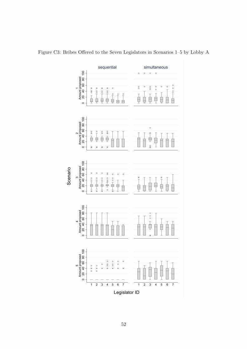
Figure C3: Bribes Offered to the Seven Legislators in Scenarios 1–5 by Lobby A

020

4060

8010

0

1Am

ount

pro

pose

d

sequential

simultaneous

020

4060

8010

0

2Am

ount

pro

pose

d

020

4060

8010

0

3Am

ount

pro

pose

d

020

4060

8010

0

4Am

ount

pro

pose

d

020

4060

8010

0

5Am

ount

pro

pose

d

1 2 3 4 5 6 7 1 2 3 4 5 6 7

Scen

ario

Legislator ID

52

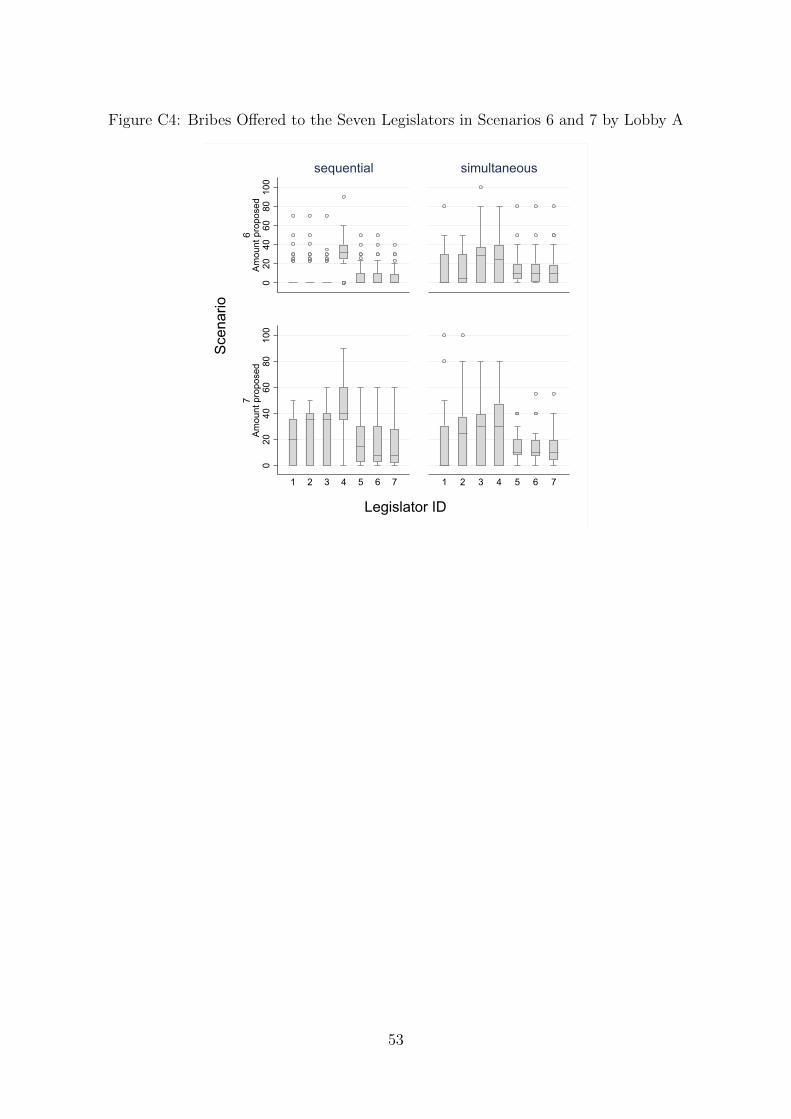
Figure C4: Bribes Offered to the Seven Legislators in Scenarios 6 and 7 by Lobby A

020

4060

8010

0

6Am

ount

pro

pose

d

sequential

simultaneous

020

4060

8010

0

7Am

ount

pro

pose

d

1 2 3 4 5 6 7 1 2 3 4 5 6 7

Scen

ario

Legislator ID

53

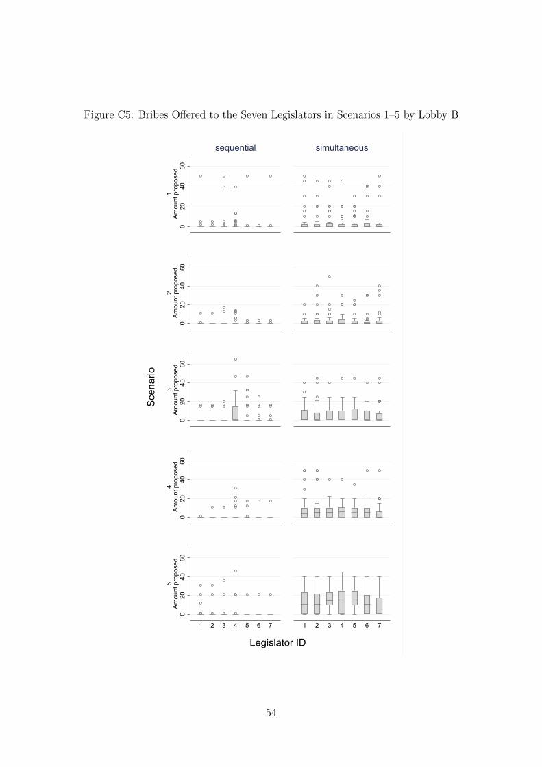
Figure C5: Bribes Offered to the Seven Legislators in Scenarios 1–5 by Lobby B

020

4060

1Am

ount

pro

pose

d

sequential

simultaneous

020

4060

2Am

ount

pro

pose

d

020

4060

3Am

ount

pro

pose

d

020

4060

4Am

ount

pro

pose

d

020

4060

5Am

ount

pro

pose

d

1 2 3 4 5 6 7 1 2 3 4 5 6 7

Scen

ario

Legislator ID

54

Figure C6: Bribes Offered to the Seven Legislators in Scenarios 6 and 7 by Lobby B

020

4060

6Am

ount

pro

pose

d

sequential

simultaneous

020

4060

7Am

ount

pro

pose

d

1 2 3 4 5 6 7 1 2 3 4 5 6 7

Scen

ario

Legislator ID

55

Figure C7: Number of Bribes by Lobby B for Scenarios with Three Legislators

0.5

11.

5

Sc1 Sc2

Mean, 95% ciEq. prediction

Sequential

Sc1 Sc2

Simultaneous0

.2.4

.6.8

1se

quen

tial

0 1 2 3 0 1 2 3

0.2

.4.6

.81

sim

ulta

neou

s

0 1 2 3Scenario 1

0 1 2 3Scenario 2

Frac

tion

Notes: The upper panel shows the means, their 95% confidence intervals based on standard errors

clustered at the subject level and the theoretical point predictions (as diamonds). The lower panel

displays the observed and theoretically predicted (in red) distributions.

56

Figure C8: Bribes Offered to the Three Legislators by Lobby A

05

1015

1Am

ount

pro

pose

d

sequential

simultaneous

05

1015

2Am

ount

pro

pose

d

1 2 3 1 2 3

Scen

ario

Legislator ID

Figure C9: Bribes Offered to the Three Legislators by Lobby B

02

46

810

1Am

ount

pro

pose

d

sequential

simultaneous

02

46

810

2Am

ount

pro

pose

d

1 2 3 1 2 3

Scen

ario

Legislator ID

57

Appendix D – Experimental Instructions and Quiz

[Below are the instructions for the seven-legislators sequential-moves treatment. Instructionsfor the other treatments were very similar and are therefore omitted here. They can be obtainedfrom the authors upon request, along with the original instructions in German.]

Overview Welcome to this experiment. We ask you not to speak with other participants during the exper-

iment and to switch off your mobile phones and other mobile electronic devices.

For your participation in today’s session, you will be paid in cash at the end of the experiment. The amount

of the payout depends in part on your decisions and partly on the decisions of other participants. It is therefore

important that you carefully read and understand the instructions before the start of the experiment.

In this experiment, every interaction between participants goes through the computers you are sitting in

front of. You will interact with each other anonymously and your decisions will only be saved along with your

random ID number. Neither your name nor the names of other participants will be made public, either today

or in future written evaluations.

Today’s session includes several rounds. Your payout amount is the sum of the earned points in all rounds,

converted into Swiss francs, plus your participation fee of CHF 5. The conversion of points into Swiss francs is

done as follows. Each point is worth 2 cents, so the following applies: 50 points = CHF 1.00.

Each participant will be paid privately at the disbursement desk, so that other participants will not be able

to see how much they have earned.

Experiment This experiment consists of 7 structurally identical rounds.

The group of two Participants are randomly divided into groups of two members each. Each round, these

groups are re-formed at random. All decisions within a round and a group of two affect only the members of

the group of two and have no influence on other groups.

The person you are forming a group with remains anonymous: that is, neither you nor the other member

learns the identity of the other member during or after the experiment.

Two group members, a committee and two alternatives In each group of two, there is a member Ma

and a member Mb. Chance decides each new round who is Ma and who is Mb, so you will most likely be Ma

in some rounds and Mb in other rounds.

In addition to Ma and Mb, there is a committee in each round and for each group, which consists of 7

committee members. The committee members are automated, that is they are played by computers and not

by other participants. The individual committee members are labeled with the labels K1–K7 and thus are

distinguishable from each other.

The committee decides by vote on one of two alternatives, A or B. A simple majority of votes for an

alternative is enough for it to be selected. That is, if alternative A receives 4, 5, 6, or 7 votes from the 7

committee members, then alternative A wins and B loses; where there are 4, 5, 6 or 7 votes for alternative B,

alternative B wins.

Your payout depends on this decision of the committee. If you are a group member Ma, you prefer alternative

A and the other group member (Mb) prefers alternative B. If you are a group member Mb, you prefer alternative

B and the other group member (Ma) prefers alternative A.

The committee members automatically receive a certain number of points from the computer each time

they vote for A or B. Below we denote by Va the number of points a committee member gets more if it votes for

A than for B. If it gets more points for a vote for B, Va is negative. The Va values of the committee members

are numbered according to their labels, so we refer to the Va value of member K2 as Va2. For example, if

58

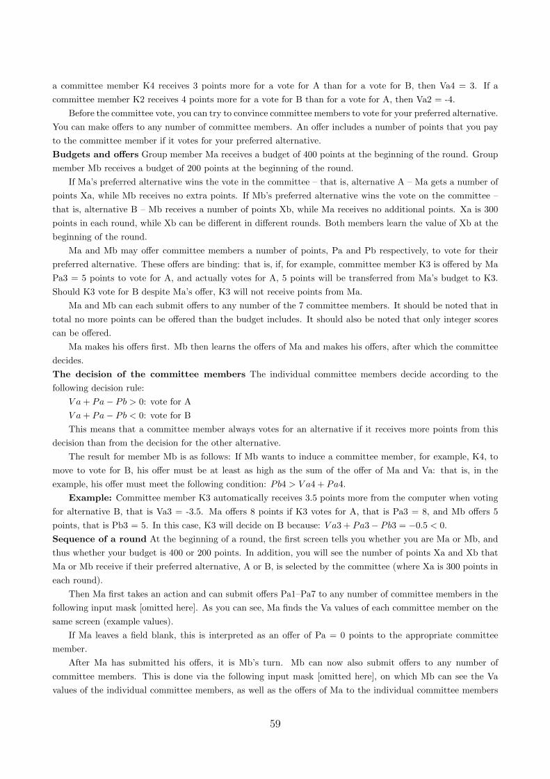
a committee member K4 receives 3 points more for a vote for A than for a vote for B, then Va4 = 3. If a

committee member K2 receives 4 points more for a vote for B than for a vote for A, then Va2 = -4.

Before the committee vote, you can try to convince committee members to vote for your preferred alternative.

You can make offers to any number of committee members. An offer includes a number of points that you pay

to the committee member if it votes for your preferred alternative.

Budgets and offers Group member Ma receives a budget of 400 points at the beginning of the round. Group

member Mb receives a budget of 200 points at the beginning of the round.

If Ma’s preferred alternative wins the vote in the committee – that is, alternative A – Ma gets a number of

points Xa, while Mb receives no extra points. If Mb’s preferred alternative wins the vote on the committee –

that is, alternative B – Mb receives a number of points Xb, while Ma receives no additional points. Xa is 300

points in each round, while Xb can be different in different rounds. Both members learn the value of Xb at the

beginning of the round.

Ma and Mb may offer committee members a number of points, Pa and Pb respectively, to vote for their

preferred alternative. These offers are binding: that is, if, for example, committee member K3 is offered by Ma

Pa3 = 5 points to vote for A, and actually votes for A, 5 points will be transferred from Ma’s budget to K3.

Should K3 vote for B despite Ma’s offer, K3 will not receive points from Ma.

Ma and Mb can each submit offers to any number of the 7 committee members. It should be noted that in

total no more points can be offered than the budget includes. It should also be noted that only integer scores

can be offered.

Ma makes his offers first. Mb then learns the offers of Ma and makes his offers, after which the committee

decides.

The decision of the committee members The individual committee members decide according to the

following decision rule:

V a + Pa− Pb > 0: vote for A

V a + Pa− Pb < 0: vote for B

This means that a committee member always votes for an alternative if it receives more points from this

decision than from the decision for the other alternative.

The result for member Mb is as follows: If Mb wants to induce a committee member, for example, K4, to

move to vote for B, his offer must be at least as high as the sum of the offer of Ma and Va: that is, in the

example, his offer must meet the following condition: Pb4 > V a4 + Pa4.

Example: Committee member K3 automatically receives 3.5 points more from the computer when voting

for alternative B, that is Va3 = -3.5. Ma offers 8 points if K3 votes for A, that is Pa3 = 8, and Mb offers 5

points, that is Pb3 = 5. In this case, K3 will decide on B because: V a3 + Pa3− Pb3 = −0.5 < 0.

Sequence of a round At the beginning of a round, the first screen tells you whether you are Ma or Mb, and

thus whether your budget is 400 or 200 points. In addition, you will see the number of points Xa and Xb that

Ma or Mb receive if their preferred alternative, A or B, is selected by the committee (where Xa is 300 points in

each round).

Then Ma first takes an action and can submit offers Pa1–Pa7 to any number of committee members in the

following input mask [omitted here]. As you can see, Ma finds the Va values of each committee member on the

same screen (example values).

If Ma leaves a field blank, this is interpreted as an offer of Pa = 0 points to the appropriate committee

member.

After Ma has submitted his offers, it is Mb’s turn. Mb can now also submit offers to any number of

committee members. This is done via the following input mask [omitted here], on which Mb can see the Va

values of the individual committee members, as well as the offers of Ma to the individual committee members

59

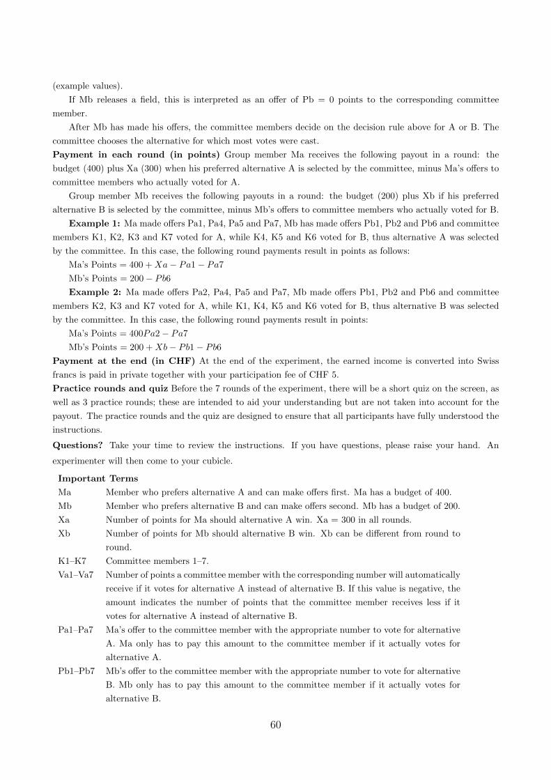
(example values).

If Mb releases a field, this is interpreted as an offer of Pb = 0 points to the corresponding committee

member.

After Mb has made his offers, the committee members decide on the decision rule above for A or B. The

committee chooses the alternative for which most votes were cast.

Payment in each round (in points) Group member Ma receives the following payout in a round: the

budget (400) plus Xa (300) when his preferred alternative A is selected by the committee, minus Ma’s offers to

committee members who actually voted for A.

Group member Mb receives the following payouts in a round: the budget (200) plus Xb if his preferred

alternative B is selected by the committee, minus Mb’s offers to committee members who actually voted for B.

Example 1: Ma made offers Pa1, Pa4, Pa5 and Pa7, Mb has made offers Pb1, Pb2 and Pb6 and committee

members K1, K2, K3 and K7 voted for A, while K4, K5 and K6 voted for B, thus alternative A was selected

by the committee. In this case, the following round payments result in points as follows:

Ma’s Points = 400 + Xa− Pa1− Pa7

Mb’s Points = 200− Pb6

Example 2: Ma made offers Pa2, Pa4, Pa5 and Pa7, Mb made offers Pb1, Pb2 and Pb6 and committee

members K2, K3 and K7 voted for A, while K1, K4, K5 and K6 voted for B, thus alternative B was selected

by the committee. In this case, the following round payments result in points:

Ma’s Points = 400Pa2− Pa7

Mb’s Points = 200 + Xb− Pb1− Pb6

Payment at the end (in CHF) At the end of the experiment, the earned income is converted into Swiss

francs is paid in private together with your participation fee of CHF 5.

Practice rounds and quiz Before the 7 rounds of the experiment, there will be a short quiz on the screen, as

well as 3 practice rounds; these are intended to aid your understanding but are not taken into account for the

payout. The practice rounds and the quiz are designed to ensure that all participants have fully understood the

instructions.

Questions? Take your time to review the instructions. If you have questions, please raise your hand. An

experimenter will then come to your cubicle.

Important Terms

Ma Member who prefers alternative A and can make offers first. Ma has a budget of 400.

Mb Member who prefers alternative B and can make offers second. Mb has a budget of 200.

Xa Number of points for Ma should alternative A win. Xa = 300 in all rounds.

Xb Number of points for Mb should alternative B win. Xb can be different from round to

round.

K1–K7 Committee members 1–7.

Va1–Va7 Number of points a committee member with the corresponding number will automatically

receive if it votes for alternative A instead of alternative B. If this value is negative, the

amount indicates the number of points that the committee member receives less if it

votes for alternative A instead of alternative B.

Pa1–Pa7 Ma’s offer to the committee member with the appropriate number to vote for alternative

A. Ma only has to pay this amount to the committee member if it actually votes for

alternative A.

Pb1–Pb7 Mb’s offer to the committee member with the appropriate number to vote for alternative

B. Mb only has to pay this amount to the committee member if it actually votes for

alternative B.

60

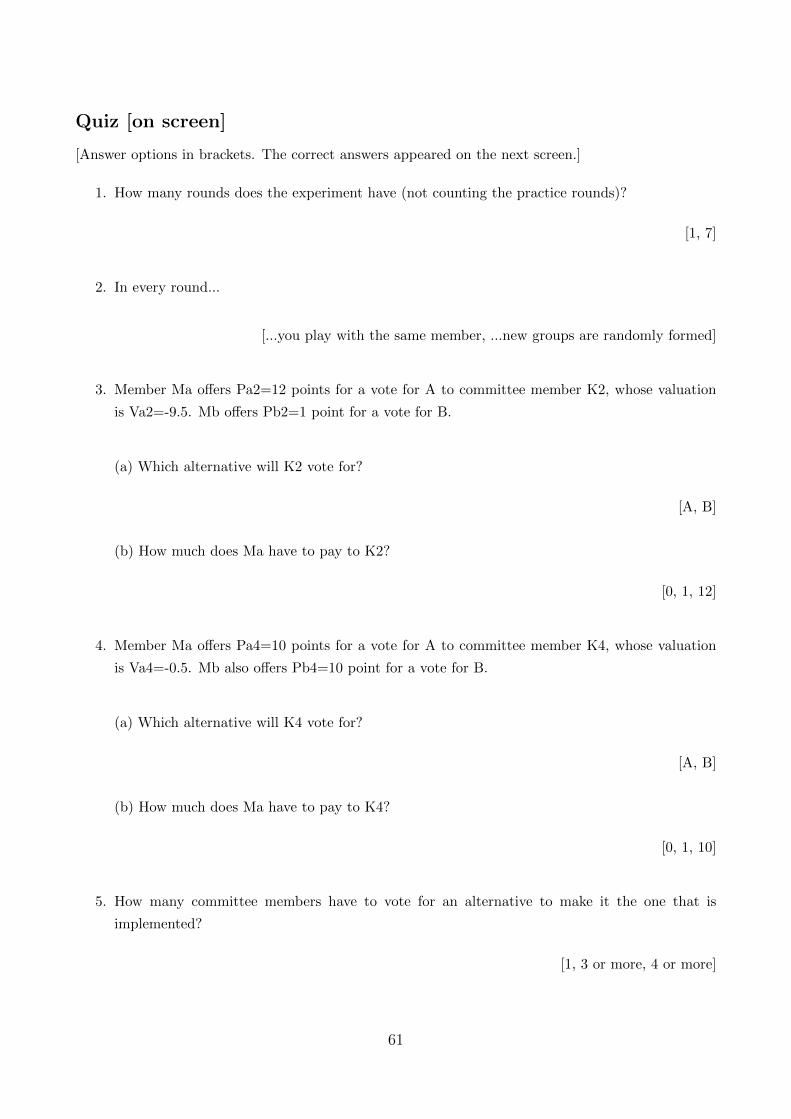
Quiz [on screen]

[Answer options in brackets. The correct answers appeared on the next screen.]

1. How many rounds does the experiment have (not counting the practice rounds)?

[1, 7]

2. In every round...

[...you play with the same member, ...new groups are randomly formed]

3. Member Ma offers Pa2=12 points for a vote for A to committee member K2, whose valuation

is Va2=-9.5. Mb offers Pb2=1 point for a vote for B.

(a) Which alternative will K2 vote for?

[A, B]

(b) How much does Ma have to pay to K2?

[0, 1, 12]

4. Member Ma offers Pa4=10 points for a vote for A to committee member K4, whose valuation

is Va4=-0.5. Mb also offers Pb4=10 point for a vote for B.

(a) Which alternative will K4 vote for?

[A, B]

(b) How much does Ma have to pay to K4?

[0, 1, 10]

5. How many committee members have to vote for an alternative to make it the one that is

implemented?

[1, 3 or more, 4 or more]

61