Embed Size (px)
Citation preview

DISCUSSION PAPER SERIES
IZA DP No. 11702
Joan Costa-FontBelen Saenz de Miera Juarez
Working Times and Overweight: Tight Schedules, Weaker Fitness?
JULY 2018

Any opinions expressed in this paper are those of the author(s) and not those of IZA. Research published in this series may include views on policy, but IZA takes no institutional policy positions. The IZA research network is committed to the IZA Guiding Principles of Research Integrity.The IZA Institute of Labor Economics is an independent economic research institute that conducts research in labor economics and offers evidence-based policy advice on labor market issues. Supported by the Deutsche Post Foundation, IZA runs the world’s largest network of economists, whose research aims to provide answers to the global labor market challenges of our time. Our key objective is to build bridges between academic research, policymakers and society.IZA Discussion Papers often represent preliminary work and are circulated to encourage discussion. Citation of such a paper should account for its provisional character. A revised version may be available directly from the author.
Schaumburg-Lippe-Straße 5–953113 Bonn, Germany
Phone: +49-228-3894-0Email: [email protected] www.iza.org
IZA – Institute of Labor Economics
DISCUSSION PAPER SERIES
IZA DP No. 11702
Working Times and Overweight: Tight Schedules, Weaker Fitness?
JULY 2018
Joan Costa-FontLondon School of Economics and Political Science and IZA
Belen Saenz de Miera JuarezLondon School of Economics and Political Science

ABSTRACT
IZA DP No. 11702 JULY 2018
Working Times and Overweight: Tight Schedules, Weaker Fitness?*
Although the rise in obesity and overweight is related to time constraints influencing
health investments (e.g., exercise, shopping and cooking time, etc.), there is limited causal
evidence to substantiate such claims. This paper estimates the causal effect of a change in
working times on overweight and obesity drawing from evidence from the Aubrey reform
implemented in the beginning of the past decade in France. We use longitudinal data from
GAZEL (INSERM) 1997-2006 that contains detailed information about health indicators,
including measures of height and weight. Taking the Alsace-Mosselle department as
a control group and a difference-in-differences strategy, we estimate the effect of a
differential reduction in working times on body weight. Our results show evidence of 0.7%
increase in average BMI an 8pp increase in the probability of overweight among blue collars
exposed to the reform. In contrast, we find no effect among white collar workers. The
effects are robust to different specifications and placebo tests.
JEL Classification: I13, J81
Keywords: obesity, overweight, working times, difference-in-differences, blue collar, white collar, Body Mass Index
Corresponding author:Joan Costa-FontDepartment of Health PolicyLondon School of Economics and Political Science (LSE)Houghton StreetLondon, WC2A 2AEUnited Kingdom
E-mail: [email protected]
* We are very grateful to Mauricio Avendano, Marcel Goldberg, Marie Zins, Dan Hamermesh, Anthony Lepinteur,
Bruce Hollingsworth, Ian Walker, Katharina Janke, Ceus Matteus, Vincent O’Sullivan, Alberto Nunez, Alexandra
Torbica, Jonathan Jones, Sonia Balotra, Marion van der Pol, and the participants of the health economics research
seminar at CERGAS, Bocconi University (December 2016, ESRC Workshop on the ‘Economics of Health Behaviours
and Health Information’ (March 2018), the University of Lancaster (April, 2017), for their comments and helpful
suggestions. The authors are responsible for any errors and omission, and the usual disclaimer applies.

3
1. Introduction The expansion of the world’s obese and overweight population is associated with energy saving,
social, and economic changes (Cutler et al., 2003; Lakdawalla and Philipson, 2009). More
generally, the rapid process of social globalization has been associated with changes in health-
related behaviours which have an impact on individual’s fitness (Costa-Font and Mas, 2016). Such
process includes the proliferation of fast foods (Maddock, 2004), as well as changes in employment
conditions, specifically longer working hours. Existing reviews and meta-studies evidence that
working time plays a role in explaining overweight and fitness (Bannai and Tamakoshi, 2014;
Sparks et al., 1994; Purgeon et al., 1997). However, the underpinning mechanisms of these
associations are unclear. Examining this matter is the main goal of this paper.
Time and energy consumed during work hours can exert an important influence on people’s fitness
(Solovieva et al., 2013). Nonetheless, the effects of working times on health behaviour, and
specifically obesity and overweight, are largely not well understood. Those effects include changes
in sedentary (non-sedentary) lifestyles among white collar (blue collar) workers, but especially
changes in time constraints that modify the opportunity cost of investing in healthy lifestyles (e.g.,
cooking fresh foods, exercising, etc.). The most common explanation of the effect of long working
hours on overweight focus on the stress response (Porter, 2010; Lee, 2017) and, more generally,
poor lifestyles when people work beyond a certain threshold (Kim et al., 2016). Economic
considerations, following a demand for health standpoint (Grossman, 1972), suggest that longer
working hours constrain the amount of time individuals spend producing healthy activities,
including food preparation, seeking preventive health care, etc. Employees compensate excessive
working time with a higher consumption of fat and sugars, and reductions on physical exercise

4
(Oliver and Wardle, 1999, Schneider and Becker, 2005). On the other hand, increased working
hours could have income effects too, namely rise labour income which can then be invested in
health production. However, income effects might well differ between white and blue collar
workers. For the latter, work exercise might well be an important source of physical exercise, hence
a reduction in working times might not produce positive health investment effects.
The literature on the effects of working time on health is scattered. Ruhm (2005) found that a
reduction in the number of hours worked has a positive impact on health among the United States
population. Similarly, using evidence of time use surveys Hammermesh (2010) found that the
amount of time eating and its spread over the day influence bodyweight and self-reported health.
Hence, relaxing time constraints should produce better health, and allow individuals to adjust to
life demands that require more exercise and lower calorie consumption. However, causal testing
of such hypothesis requires an exogenous variation in working times among a control group.
Verneill (2016), drawing from the French health survey to examine the Aubrey reform by looking
at the difference between large and small firms, found an effect of working time reductions on
smoking, alcohol consumption and physical activity, but other studies find no evidence of an effect
(Jang et al., 2013). Hence, we need further understanding of the effect of exogenous changes in
working times. Measuring the effect of a reduction in working times on obesity is crucial for policy
purposes, and specifically to understand the underlying mechanisms to fight the so-called obesity
epidemic.
The OECD (1998) has identified an overall downward trend in working time. This reduction does
not necessarily entail homogeneous effects across the entire population, however. Blue collar
workers might benefit from shorter working days, but at the same time they might see one specific

5
source of fitness reduced. In contrast, white collar workers might benefit from more free time,
especially if such extra time is devoted to health-related activities –although white collar jobs tend
to encompass more employment flexibility.
This paper exploits a unique natural experiment, namely the reduction of working time
implemented in France in 2001. Askenazy (2013) estimates that this reform resulted in an overall
7% reduction of working time from 1995 to 2003 compared to 3% elsewhere in the EU. An
important feature of the French reform lies in that it primarily affected individuals who worked for
large companies. Indeed, we take advantage of a unique dataset that draws upon employees of
Electricité de France-Gaz de France (EDF-GDF), a large company (hence affected by the reform)
created after the second WW by the French government to provide energy1. Given that EDF -GDF
employs individuals both in administrative and manufacturing positions, we can distinguish blue
and white collar workers. We can also distinguish individuals who work in energy production and
distribution; the latter sector was liberalised after 2000. Finally, given that the company is
regionally heterogeneous we can identify employees by region, which is essential for the
identification strategy adopted.
If obesity results from the excesses of modern life where individuals have limited time to cook
their meals, more leisure time should provide individuals with time to prepare meals, and more
generally less pressure. Failure to find evidence of obesity declines derived from reductions in
working times would be suggestive of other factors playing out in explaining the onset of obesity.
1 Although from 2000-2004 there was a market liberalization to introduce competition in the distribution and energy transport sector, the effect did not influence the energy production. In our dataset, we are able to distinguish such effects.

6
Similarly, a reduction of working times might impact individual’s stress, which in turn can reduce
the probability of smoking and drinking, especially among men. Policy implications of this
question are key, in that if positive, they would suggest that obesity results at least in part from
changes in working conditions originated from a more global word. Likewise, evidence of
reductions on smoking and alcohol intake would suggest that working time reforms can give rise
to second-order effects.
Our empirical strategy consists in a difference-in-differences especification that exploits the
variation across individuals who are white and blue collar workers, and specifically the variation
in one region that has had historically different labour regulations and where the timing of the
reform was different from the rest of France. In particular, we draw on the methodology proposed
by Chemin and Wasmer (2009) that uses the specificities of Alsace-Moselle local regulations to
build a control group. In such department, the legislation is inherited from the German presence
between 1871 and 1918 and implies that workers have two extra holidays, which are included in
the calculation of non-working time. Therefore, the reduction in working time was smaller in this
region than in the rest of the country. For managers, the reform mainly consisted in an expansion
of holidays without pay cuts (Askenazy, 2013), so it appears important to run a specific analysis
for white collar workers.
Our findings suggest no evidence of changes in obesity immediately after the implementation of
the reform. In contrast, we find evidence of an increase in overweight among blue collars. The
effect was not significantly heterogeneous across age, gender, spousal employment status, and
socio-economic groups as we report below. The presence of children in the household, however,
does absorb the baseline effect on overweight among blue collars, which suggests a potential

7
substitution effect of working time for child care. The structure of the paper is as follows. The next
section provides an overview of the relevant literature. Section three describes the institutional
background. Section four reports the empirical strategy. Section five contains the results, and a
final section concludes.
2. Working Times and Health
2.1 Opportunity Costs and Time Savings
Some evidence links obesity and overweight to higher opportunity costs of time in a modern
lifestyle. Accordingly, under significant time constraints a number of studies emphasise the role
of fast foods in explaining the rise in obesity and overweight (Cutler et al., 2003; Chou et al.,
2004), as well as the development of Walmart supercenters (Courtemanche & Carden 2011).
Some of such effects are attributed to food prices that attract less affluent individuals into
consuming high-calorie foods. However, another effect results from time savings, which is
especially important under long working hours and competing time allocation activities.
Nonetheless, the study of such time effects on health requires the examination of reforms that
affect the individual’s allocation of time. We specifically rely on the role of a unique regulation
that reduced working times in France as explained in the following section.
2.2 Working conditions and health
The impact of working conditions on health has received some attention in the literature.
Drawing on evidence from South Korea, Kim et al. (2008) found that labour market precarious
conditions have deteriorated mean health. Similarly, other studies have found that both overtime
and unpredictable work hours are associated with lower well-being (Golden et al., 2006; Scholars

8
et al., 2017). That is, there seem to be direct consequences of extended hours for non-work life,
which in turn are deemed to reduce individual’s well-being. Some studies have also found that
long or unsocial hours affect family and social life alongside physical health (Artazcoz et al.,
2013).
A reduction in working times might be hypothesized to allow more time to produce health or
prevent ill health: it can result in less work pressure without affecting leisure time. Alternatively,
the extra leisure time will be allocated to healthy and unhealthy activities depending on
individuals’ unobserved preferences, which could vary by age cohort, gender, educational
attainment, household size, and commuting time, among other factors. At the same time, lower
working times might mean only half day off every week, or a day off every second week, or a
week off every ten rather than a reduction in an hour a day. Finally, while the reduction of
working time was hypothesised to produce job creation through work-sharing (Crepon &
Kramarz, 2002, Chemin & Wasmer, 2009), Esteao and Sa (2008) found that the reduction of the
workweek in France from 39 to 35 hours in 2000-2002 had no effect on aggregate employment,
though it did increase job turnover. The actual effect of working time reductions on health is thus
an empirical questions that this study attempts to address.
2.3 Effects of Working Time on Wealth and Well-being
Although job creation is the main purpose of working time reductions, other side effects may
include an improvement in wealth and well-being of those exposed to the reforms. However, the
evidence of reduced working times on well-being is not conclusive. One the one hand, some
studies indicate that a reduction of working times might increase the stress and work accidents of
workers attempting to perform a similar workload in lesser time (Rudolf, 2014). In contrast,

9
Hamermesh et al. (2017) found that Japanese and Korean reforms that reduced working times did
increase life satisfaction of those exposed. Similarly, Lepinteur (2016) drawing on evidence from
France and Portugal from large and small firms found positive effects on life satisfaction.
3. Institutional Background
The French labour market reform has been largely aiming at expanding employment. One of the
policies formulated back in 1981 by the French left wing movement was the reduction of week
working times (réduction du temps du travail) to 35 hours (Askenazy, 2013). In practice, the
agreement reduced working times to 39 hours, so that only work in excess of 39 would be paid
overtime, and the subsidy for reduced working times was increased. In 1996 a new conservative
government incentivised the voluntary reduction of 10-15% of working times, but it was not until
a new, and unexpected socialist led coalition government was elected in 1997 with the purpose of
reducing unemployment that the original idea of a 35-hour working week was back in the agenda
as a way of ‘work sharing’. The proposal attempted to reduce working times to 35 hours a week
with full wage, but it would primarily apply to large companies (small companies were allowed a
longer transition period) that would receive a generous tax compensation for the resulting rise in
labour costs.
The working time regulation, referred as Aubry law, was passed in two blocs. The first bloc was
passed in June 1998 (Aubry I), which reduced the legal working time limit from 39 to only 35
hours per week from 1st January 2000 for companies with more than 20 employees such as EDF-
GDF. Hours worked beyond 35 would be treated as overtime hours subject to a 25% hourly rate
bonus and a maximum of 130 per employee per year. The latter would result from collective

10
agreements between the company and trade unions. Hence, the regulation appears to be an
important exogenous mechanism to identify the pure substitution effects of working time
reductions, as there was no income effect. Although there might have been organizational
changes around the same time, examining a single company such as EDF-GDF could help the
identification of these effects.
However, the specifics of the reform were only included in the second bloc passed in 2000
(Aubry II). During the transition period there were intense negotiations that resulted in the
implementation of 16,000 annual work hours as a legal norm, and allowed some flexibility for the
companies so that they could ask their employees to work more hours in some weeks and
compensate with fewer hours in other weeks. Hence, the standard workweek was reduced from
39 to 35 hours first on a voluntary basis coupled with incentive schemes conditional on
employment creation (Robien act 1996, Aubry I act 1998), and then on a compulsory basis
(Aubry II act 2000). The costs of the reform were originally estimated at 200,000 dollars per job
created, which were supposed to be funded from alcohol and tobacco tax revenues. However, the
fast adoption shifted up the costs, which required an injection from the unemployment fund
(UNEDIC). This was deemed appropriate given that the reform was expected to reduce
unemployment, and hence the outlays of unemployment benefits.
Although the Aubry law initially concerned private employers, it was also implemented in the
public sector; hence, the so-called privatization of EDF-GDF after 2000 would have produced no
effects on working times. However, there was very large heterogeneity in the implementation
across sectors (Askenazy, 2013); therefore it appears convenient to examine a dataset that
contains records of the same sector and activity to analyse the effects of such reform.

11
After the defeat of the incumbent socialist party in 2002, the law was not implemented in small
companies and the maximum extra hours were increased from 180 to 240. After the 2007 defeat
in the presidential elections the law was repealed.
During the period of implementation of the Aubry law there were very limited health reforms in
the country. Most of these reforms aimed at reducing out-of–pocket health care payments and
improving geographical access. However, France is among the OECD countries for which public
financing of health care expenditure is the highest (Chevreul et al., 2015).
4. Empirical Design
4.1 Data
This study employs GAZEL data, a dataset managed by the French National Institute for Health
and Medical Research (INSERM) in collaboration with the occupational health and human
resource departments of EDF-GDF. The GAZEL Cohort Study was set up in 1989 among EDF-
GDF workers. It is an open epidemiologic laboratory characterized by a broad coverage of health
problems and determinants, accessible to the community of researchers. At inception, the
GAZEL Cohort Study included 20,624 volunteers then aged from 35 to 50 years (15,010 men and
5,614 women). The cohort is broadly diverse in terms of social, economic and occupational
status, health and health-related behaviour.
The data, routinely collected, cover diverse dimensions and come from different sources: annual
self-administered questionnaires (for morbidity, lifestyles, life events, etc.); personnel department

12
of EDF-GDF (for social, demographic, and occupational characteristics); EDF-GDF Special
Social Insurance Fund (for sickness absences and cancer and ischemic heart disease registries),
EDF-GDF occupational medicine department (for occupational exposure and working
conditions), Social Action Fund (for healthcare utilization), Health Screening Centers (for
standardised health examination and the constitution of a biobank), and the National Death
Register (for causes of death). Follow-up has been excellent, and the number of subjects lost to
follow-up is exceptionally low; active participation through the self-administered questionnaire is
also large.
In particular, GAZEL database contains yearly self-reported data on weight and height, which
was used to calculate the body mass index (BMI):
BMI𝑖𝑖 =weightiheighti2
where weight𝑖𝑖 is the weight of individual i measured in kilograms and heighti2 is the square of
the height of individual i measured in meters. Perceived health status and smoking behaviour is
also collected on an annual basis. The former is measured with a scale from 1 to 8, where 1 is
very good and 8 is very poor; the latter indicates whether the person smokes, and if so, the
quantity of cigarettes smoked per day. Monthly household income is measured at the cohort
inception. The original nine categories were grouped into three that roughly correspond to
income terciles (low, middle and high). Other information employed in the analyses include age,
sex, educational attainment, spouse’s employment status and an indicator of the presence of
children in the household. We also distinguish white collar from blue collar workers, and those in
the distribution from those in the production sector to exploit the variation in the type of
employment together with regional differences (see section 4.2). This is particularly relevant as

13
the activities of both blue collar workers and those in the production sector entail more physical
activity. Moreover, this distinction allows taking into account possible changes in working
conditions in the distribution sector after the liberalisation of this part of EDF-GDF in the
beginning of the past decade. Unfortunately, we cannot identify the number of hours worked per
individual but other studies have shown that the Aubry reform effectively reduced working times
(e.g., Chemin and Wasmer, 2009).
Only respondents who worked during the reference period (1997-2006), with complete
information, were considered in the analysis. Residents of territories were excluded. As displayed
in Table 1, we were left with an unbalanced panel that contains 49,830 individual-wave
observations (see Table A1 for a description of the number of observations by year). Figure A0
depicts the French departments where the Alsace-Moselle region can be identified in the extreme
right.
[Insert Table 1 about here]
4.2 Empirical Strategy
Unlike other studies examining the effect of the Aubry reform, we employ data from a single,
large company. Hence, we cannot rely on analysing the differential effects between large and
small companies as other studies do (e.g. Berniell and Bietenbeck, 2017). Instead, we follow
Chemin and Wasmer (2009) who estimate the causal effect of the Aubry reform by comparing
Alsace-Moselle to the rest of France between 2001 and 2002. Indeed, the Alsace-Moselle region
attenuated the impact of the Aubry reform by including two public holidays (December 26 and
Good Friday) as part of the reduction in working time. In other words, this region reduced

14
working times by two days less, namely 16 hours of work per year. The 35-hour reform
corresponded to a reduction of four hours per week throughout the 46-week workyear, for a total
reduction of 184 hours. Therefore, there was a 9% variation in the impact of the 35-hour reform
in Alsace-Moselle as opposed to the rest of the country. This regional disparity in the
implementation of the Aubry reform, however, was only in effect between 2001 and 2002, since
the local council forbade considering public holidays as part of the reduction in working time
from 2003.
The difference-in-differences model estimated was the following:
BMIidt = αd + δt + β1(treated ∗ 2001 − 2002)idt + β2(treated ∗ −2000)idt
+ β3(treated ∗ 2003 − 2006)idt + γXidt + εidt
where BMIidt is the body mass index of individual i, from department d, at year t; αd are
department fixed effects; δt are year fixed effects; (treated ∗ 2001 − 2002)idt, (treated ∗
1999 − 2000), and (treated ∗ 2003 − 2006)idt are binary variables that take the value of 1 if
individual i lives in departments other than Alsace-Moselle (i.e. treated departments) in 2001-
2002, 1999-2000, and 2003 or later, respectively; and Xidt refer to individual-level controls,
namely, sex, age and education. The reference period is therefore 1997-1998. The coefficient of
interest, β1, indicates the relative change in body mass index of individual i from the control
region after the reform. The coefficient β2 allows testing the parallel trend assumption. Standard
errors were clustered at the department level. The models were also estimated using binary
dependent variables, overweight and obesity. The former takes the value of 1 if the body mass
index is 25 or more, while the latter takes the value of 1 if the body mass index is 30 or more.

15
Our main focus of interest lies in examining the entire sample of workers, as well as the specific
effects on two different samples defined by type of job, namely white and blue collar jobs. The
rationale for this distinction is that blue collar jobs mainly entail physically intensive activities
(e.g. technicians), whilst white collar jobs predominantly entail mentally intensive activities (e.g.
administrative). In other words, blue collar workers main physical activity is related to their job,
while white collar workers physical activity might well be unrelated to their jobs. Hence, we
expect different effects, even in opposite direction between the two types of workers. The
definition of blue and white collars was taken from GAZEL databook.
Furthemore, we examine additional sources of heterogeneity that do not constitute different types
of samples, such as whether the job was in the distribution or in the production unit of the energy
sector, household income and spouse’s employment interactions, as well as gender and age
effects. In addition, the second part of our empirical strategy addresses potential mechanisms, and
more specifically, the role of children in the household. Given that the additional time gained
with the Aubry reform could be spent on multiple competing activities including child care, we
examine the specific heterogenenity resulting from the presence of children in the household. We
also analyse potential effects on health and health behaviours, namely self-reported health and
smoking. Finally, our empirical strategy involves some placebo tests that use as control areas of
the country that were affected by the reform to see if there are any random effects emerging.
Specifically, we examine two regions, Ille de France and Auvergne, which are geographically far
from Alsace-Moselle and hence unlikely to be affected by factors different to the Aubry reform
that may be present in neighbouring regions.

16
4.3 Pre-reform Trends
As preliminary evidence of the suitability of the identification strategy, we examine pre-reform
trends of outcome variables. Figure 1 reports the trends in overweight and body mass index for
the period 1997 – 2006 for the entire sample, as well as for blue and while collar workers. It
becomes apparent that pre-treatment trends (up to 2001) were comparable between Alsace-
Moselle and the rest of France, but differed around the treatment years (2001-2002) for both
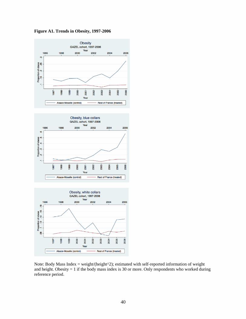
overweight and body mass index. Similar trends are reported for obesity in the appendix in
Figure A1.
[Insert Figure 1 about here]
Specifically, when we split the sample we find evidence of differential impacts of the reform in
both overweight and BMI between blue and white collars, and between Alsace-Moselle and the
rest of France. However, pre-trends seem to be consistently similar across both types of regions.
This is confirmed in formal testing (see the estimates of coefficient β2 in section 5.1 below).
Furthemore, we also provide estimates without pre-trends so as to examine the effects of
controlling for pre-existing trends.
5. Results
5.1 Baseline Results
To estimate the effect of an ameliorated exposure to the Aubry reform (reduced working times, or
henceforth the treatment) we examine changes in Body Mass Index and overweight for the total
sample, and especially, for the subsample of blue and white collar workers. The rationale for

17
examining different samples lies in the fact that blue collar jobs mainly entail physically intensive
activities, and hence can be reasonably considered a separate group of individuals.
Table 2 reports the estimates for both BMI and overweight for the entire sample and the
subsample of blue and white collar workers. Importantly, we find that although there was no
significant effect overall, blue collar workers in treated areas (where the 35-hour reform was fully
enforced) had a BMI 0.17 units higher than their counterparts in control areas (Alsace-Moselle).
Given that the average BMI is 25.5 (Table 1), such an effect entails a 0.7% increase in BMI.
Similarly, we find that the reform significantly increased the probability of overweight for the
entire sample in 2.7pp and and 8pp among the sample of blue collar workers. These results were
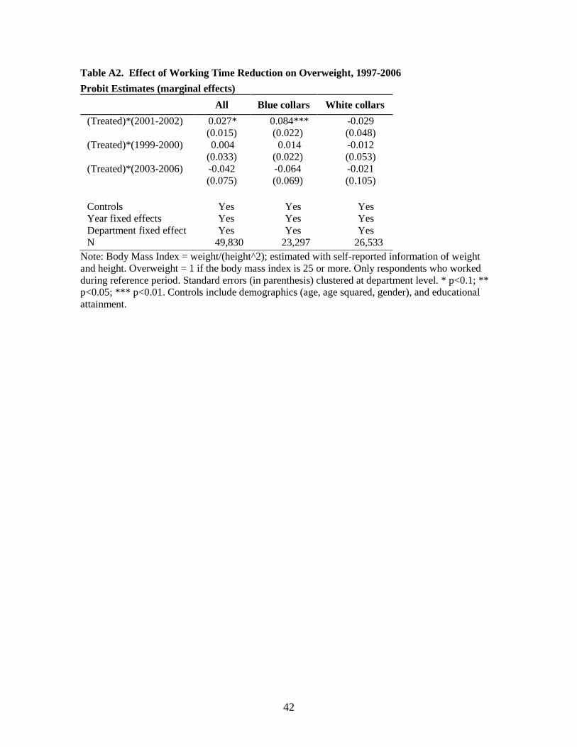
estimated using ordinary least squares (OLS) but not significant difference is found when probit
models are employed (Table A2). We find no effect among the sample of white collar workers.
Table A3 reports similar estimates for obesity, and suggests no evidence of an effect. Tables B1-
B3 in the Appendix provide the full estimates with the coefficients for all the controls. Results
without controls for overweight among blue collars show a consistent picture (columns 2 and 5,
Table 2).
[Insert Table 2 about here]
5.2 Robustness Checks
Next, we present the estimates of Table 2 but excluding pre-treatment trends in Table 3.
Importantly, we find that although the effect on BMI do not emerge as significant anymore, the
effects on overweight are barely unchanged for both the entire sample and the subsample of blue
collar workers. Specifically, the effect is 2.2pp and 7.3pp for the entire and blue collar samples,

18
respectively. Consistently, no significant effect is found among white collar workers. Tables B4-
B5 in the Appendix provide estimates with the coefficients for all the controls.
Section 5.3 below explores spousal employment status, household income, and the activity sector
(distribution vs. production) as potential sources of heterogeneity, but we first included those
variables as additional controls to assess the validity of the results presented in Table 2. Estimates
are found to barely change, however (Tables C1-C6 in the Appendix).
[Insert Table 3 about here]
Finally, to test the validity of the identification strategy employed, we selected two densely
populated regions to conduct a placebo test, namely Ile de France in the north and Auvergne in
the south. This test basically consisted of replacing Alsace-Moselle, the control group, by each of
the other regions. As shown in Table 9, the results were not statistically significant, which
supports the methodological approach employed.
[Insert Table 9 about here]
5.3 Heterogeneity of the Results
5.3.1 Area of Activity
Given that the distribution sector of EDF-GDF underwent a liberalization process around the
same time of the Aubry reform, one could expect heterogenous effects depending on the area of
activity individuals were working on. Hence, we first report estimates of triple interactions of the

19
treatment and the area of activity. Table 4 displays such estimates and suggests that the results are
only significant for the production area; specifically, slightly larger coefficients are observed, 3pp
and 9pp for the entire sample, and the subsample of blue collar workers, respectively.
Furthemore, Tables D1 and D2 in the Appendix provide additional estimates where we split the
sample by area of activity. Importantly, when the effect fo the reform is estimated among blue
collars working in the production area, we see an increase of 32pp in BMI, which acrues to a
12% increase. Moreover, we find that for both distribution and production areas an effect of the
reform on overweight ranging between 8-9pp. However, among the distribution sector we find a
negative effect among white collar workers consistent with the idea of a health investment effect
of extra time but only applicable among the distribution sample alone.
[Insert Table 4 about here]
5.3.2 Spousal Employment Status and Income Effects
The effects of the French reform might have been heterogeneous depending on respondents’
marital status, and more specifically, on whether the spouse is employed. A reduction in working
times of one spouse might not necessarily entail an equivalent reduction in the other spouse’s
working time if the latter was working in a smaller company and hence was not affected by the
reform. Table 5 in Panel A provides estimates that suggest that the effect does not vary by
spousal employment.
[Insert Table 5 about here]

20
Another potential source of heterogeneity is respondents' income. One could hypothesize that
more affluent individuals might not respond to a working time reduction in the same way as their
lower income counterparts. Panel B of Table 5 reports the results of such interaction, and indicate
no evidence of this source of heterogeneity. Full estimates with all controls are reported in tables
E1-E4 in the Appendix.
5.3.3 Gender and Age Heterogeneity
The last important sources of heterogeneity considered are gender and age, which we report in
Table 6 and Tables E5-E8 (in the Appendix). It could well be the case that old age individuals
exhibited a different reaction, or that men and women exhibited different preferences with
regards to health production. However, estimates sugest no evidence of an heterogeneous effect
on both gender and age.
[Insert Table 6 about here]
5.4 Mechanisms
Next, we examine the potential mechanisms driving the effect of the French reform on
overweight. Specifically, we identified two mechansims: the presence of children in the
household and the potential effect of the reform on health and health behaviour.
The presence of children in the household could arguably pick up a potential substitution effect of
working time for child care. To examine this question, Table 7 reports evidence of the
heterogeneity of our estimates derived from the presence of children. Estimates suggest that the

21
presence of children does indeed absorb our baseline results. Again, estimates containing the full
list of controls are reported in the Appedix (Tables E9 and E10).
[Insert Table 7 about here]
An alternative mechanism could be through specific effects on health, or health behaviours such
as smoking. The latter is found to exert some influence on the probability of overweight and
obesity (Gruber and Frakes, 2006). Nonetheless, Table 8 suggests no evidence of an effect of the
reform on self-assessed health, or in both the internal and external margins of smoking. The full
list of controls are reported in Tables F1-F4 in the Appendix.
[Insert Table 8 about here]
6. Conclusion
This paper has examined the effect of the French working time reduction on overweight. We
have taken advantage that one department (Alsace-Moselle) exhibited a reduced implemention of
the reform. Against the hypothesis of heatlh investment effects, we find that reduced working
times increase overweight among blue collar workers and exert no effect on the rest (0.7%
increase in BMI) .Our estimates suggest that blue collar workers in treated areas (where the 35-
hour reform was fully enforced) had a BMI 0.17 units higher and a probability of overweight 8pp
higher than their counterparts in control areas (Alsace-Moselle). However, we find no effect on
obesity, in part given the significant genentic influences and that small working time

22
interventions might not change significantly the environment on which individuals make
decisions .
Our findings also indicate that individuals working in the production sector mainly drives the
increasing overweight, and that reduced working time was employed in reducing external
childcare rather than increasing leisure time. These results are consistent with other evidence on
the French reform (Goux et al., 2014), and overall suggest that policies to reduce waiting times
alone does not necessarily produce better fitness, either because they do not modify the
environment (e.g., individuals take more holidays etc.), or because the produce counterproductive
incentives in a population (blue collar workers) for who their job related physical activity is its
primary form of exercise. One potential way out is to make reduced time conditional on exercise,
or to combine working time reduction with subsidies for healthy lifestyles.

23
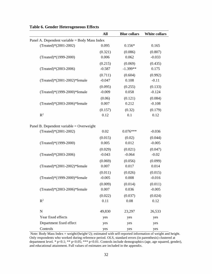
References
Artazcoz, L., Cortès, I., Escribà-Agüir, V., Bartoll, X., Basart, H., & Borrell, C. (2013). Long working hours and health status among employees in Europe: Between-country differences. Scandinavian Journal of Work, Environment & Health, 39: 369–378. Askenazy, P. (2013). Working time regulation in France from 1996 to 2012. Cambridge Journal of Economics, 37: 323–347. Bannai, A., & Tamakoshi, A. (2014). The association between long working hours and health: A systematic review of epidemiological evidence. Scand J Work Environ Health, 40: 5-18. Berniell, I., & Bientenbeck, J. (2017). The effect of working hours on health. IZA DP nº 10524. Chevreul, K., Berg Brigham, K., Durand-Zaleski I., & Hernández-Quevedo, C. (2015). France: Health system review. Health Systems in Transition, 17(3): 1–218. Chou, S., Grossman, M., & Saffer, H. (2004). An economic analysis of adult obesity: Results from the Behavioral Risk Factor Surveillance System. Journal of Health Economics, 23(3): 565–587. Courtemanche, C., & Carden, A. (2011). Supersizing supercenters? The impact of Walmart Supercenters on body mass index and obesity. Journal of Urban Economics, 69(1): 165–181. Crépon, B., & Kramarz, F. (2002). Employed 40 hours or not employed 39: Lessons from the 1982 mandatory reduction of the workweek. Journal of Political Economy, 110(6): 1355–1389. Cutler, D. M., Glaeser, E. L., & Shapiro, J. M. (2003). Why have Americans become more obese? The Journal of Economic Perspectives, 17(3): 93–118. Chemin, M., & Wasmer, E. (2009). Using Alsace-Moselle local laws to build a difference-in-differences estimation strategy of the employment effects of the 35-hour workweek regulation in France. Journal of Labor Economics, 27(4): 487–524. Estevão, M., & Sa, F. (2008). The 35-hour workweek in France: Straightjacket or welfare improvement? Economic Policy, 23(55): 418–463. Golden, L., & Wiens-Tuers, B. (2006). To your happiness? Extra hours of labor supply and worker well-being. The Journal of Socio-Economics, 35(2): 382–397. Gruber, J., & Frakes, M. (2006). Does falling smoking lead to rising obesity?. Journal of Health Economics, 25(2): 183–197.
24
Goux, D., Maurin, E., & Petrongolo, B. (2014). Worktime Regulations and Spousal Labor Supply. American Economic Review, 104 (1): 252–76. Jang, T. W., Kim, H. R., Lee, H. E., Myong, J. P., & Koo, J. W. (2013). Long work hours and obesity in Korean adult workers. J Occup Health, 55(5): 359–366 Kim, M. H., Kim, C. Y., Park, J. K., & Kawachi, I. (2008). Is precarious employment damaging to self-rated health? Results of propensity score matching methods, using longitudinal data in South Korea. Social Science & Medicine, 67(12): 1982-1994. Kim, B. M., Lee, B. E., Park, H. S., Kim, Y. J., Suh, Y. J., Kim, J., Shin, J. Y., & Ha, E. H. (2016). Long working hours and overweight and obesity in working adults. Annals of Occupational and Environmental Medicine, 28(1): 36. Hamermesh, D. (2010). Incentives, time use and BMI: The roles of eating, grazing and goods. Economics and Human Biology, 8: 2–15. Hamermesh, D. S., Kawaguchi, D., & Lee, J. (2017). Does labor legislation benefit workers? Well-being after an hours reduction. Journal of the Japanese and International Economies, 44: 1–12. Lee, K., Suh, C., Kim, J.-E., & Park, J. O. (2017). The impact of long working hours on psychosocial stress response among white-collar workers. Industrial Health, 55(1): 46–53. Lepinteur, A. (2016). The shorter workweek and worker wellbeing: Evidence from Portugal and France. PSE Working Papers nº 2016-21. Maddock, J. (2004). The relationship between obesity and the prevalence of fast food restaurants: state-level analysis. American Journal of Health Promotion, 19(2): 137–143 Oliver, G., & Wardle, J. (1999). Perceived effect of stress on food choice. Physiol Behav 66: 511–515. Porter, J.S., Bean, M.K., Gerke, C.K., & Stern. (2010). M. Psychosocial factors and perspectives on weight gain and barriers to weight loss among adolescents enrolled in obesity treatment. J Clin Psychol Med Settings, 17(2): 98–102. Rudolf, R. (2014). Work shorter, be happier? Longitudinal evidence from the Korean five-day working policy. Journal of Happiness Studies, 15(5): 1139-1163. Ruhm, C. (2005). Healthy living in hard times. Journal of Health Economics, 24(2): 341–363. Scholarios, D., Hesselgreaves, H., & Pratt, R. (2017). Unpredictable working time, well-being and health in the police service. The International Journal of Human Resource Management, 28:16, 2275–2298.

25
Schneider, S., & Becker, S. (2005). Prevalence of physical activity among the working population and correlation with work- related factors: Results from the first German national health survey. J Occup Health, 47: 414–423. Solovieva, S., Lallukka, T., Virtanen, M., & Juntura, E. (2013). Psychosocial factors at work, long work hours and obesity: a systematic review. Scand J Work Environ Health, 39: 241–258. Sparks, K., Cooper, C., Fried, Y., & Shirom, A. (1997). The effects of hours of work on health: A Meta - analytic review. J Occup Organ Psychol, 70: 391–408.

26
Table 1. Sample characteristics at first interview (standard errors in parenthesis) Characteristics Total Alsace-Moselle
(control) Rest of France
(treated) n=11,607 n=352 n=11,255
Age 51.1 (.028) 51.2 (.146) 51.1 (.028) Sex Male 74.0% (.004) 84.4% (.019) 73.7% (.004) Female 26.0% (.004) 15.6% (.019) 26.3% (.004) Education Basic certificate 4.2% (.002) 2.0% (.007) 4.3% (.002) Junior secondary certificate 13.6% (.003) 5.7% (.012) 13.9% (.003) Baccalaureate 7.9% (.003) 8.5% (.015) 7.9% (.003) Certificate of professional competence 27.2% (.004) 38.6% (.026) 26.9% (.004) Vocational certificate 23.1% (.004) 25.3% (.023) 23.0% (.004) Undergraduate degree 7.1% (.002) 8.2% (.015) 7.1% (.002) Other academic degree 14.4% (.003) 8.8% (.015) 14.6% (.003) Other diploma 2.4% (.001) 2.8% (.009) 2.4% (.001) Work position White collar 46.8% (.005) 40.9% (.026) 47.0% (.005) Blue collar 53.2% (.005) 59.1% (.026) 53.0% (.005) Body mass index 25.5 (.032) 26.3 (.181) 25.4 (.033)
Notes: Body mass index = weight/(height^2); estimated with self-reported information of weight and height. Only respondents who worked during reference period. n = sample size.

27
Table 2. Effect of working time reduction on body mass index and overweight, 1997-2006
All Blue collars
White collars All Blue
collars White collars
1 2 3 4 5 6 Panel A. Dependent variable = Body Mass Index
(Treated)*(2001-2002) -0.028 -0.021 0.267 0.077 0.170** 0.104 (0.309) (0.08) (0.741) (0.321) (0.084) (0.819) (Treated)*(1999-2000) 0.001 0.034 -0.001 0.003 0.07 -0.092 (0.2) (0.058) (0.419) (0.213) (0.062) (0.441) (Treated)*(2003-2006) -0.49 -1.613*** 0.448 -0.584 -1.338** 0.095 (0.662) (0.602) (0.945) (0.709) (0.589) (1.003) R2 0.02 0.03 0.02 0.12 0.10 0.12
Panel B. Dependent variable = Overweight (Treated)*(2001-2002) 0.01 0.054*** -0.005 0.023* 0.078*** -0.029 (0.012) (0.019) (0.034) (0.014) (0.019) (0.044) (Treated)*(1999-2000) 0.003 0.009 -0.001 0.003 0.013 -0.012 (0.027) (0.018) (0.046) (0.029) (0.02) (0.048) (Treated)*(2003-2006) -0.025 -0.090* 0.028 -0.04 -0.054 -0.023 (0.063) (0.052) (0.093) (0.068) (0.054) (0.1) Year fixed effects yes yes yes yes yes yes Department fixed effect yes yes yes yes yes yes Controls no no no yes yes yes R2 0.02 0.03 0.02 0.12 0.10 0.12 N 49,830 23,297 26,533 49,830 23,297 26,533 Year fixed effects yes yes yes yes yes yes Department fixed effect yes yes yes yes yes yes Controls no no no yes yes yes
Note: Body Mass Index = weight/(height^2); estimated with self-reported information of weight and height. Overweight = 1 if the body mass index is 25 or more. Only respondents who worked during reference period. OLS, standard errors (in parenthesis) clustered at department level. * p<0.1; ** p<0.05; *** p<0.01. Controls include demographics (age, age squared, gender), and educational attainment. Full values of the estimates are included in the appendix.

28
Table 3. Alternative Specification without Pre-Treatment Trends All Blue collars White collars Panel A. Dependent variable = Body Mass Index (Treated)*(2001-2002) 0.076 0.142 0.142 (0.243) (0.091) (0.664) (Treated)*(2003-2006) -0.585 -1.366** 0.132 (0.626) (0.57) (0.832) R2 0.12 0.10 0.12 Panel B. Dependent variable = Overweight (Treated)*(2001-2002) 0.022*** 0.073*** -0.024 (0.008) (0.02) (0.025) (Treated)*(2003-2006) -0.041 -0.059 -0.018 (0.056) (0.047) (0.081) Year fixed effects yes yes yes Department fixed effect yes yes yes Controls yes yes yes R2 0.11 0.08 0.12 N 49,830 23,297 26,533 Year fixed effects yes yes yes Department fixed effect yes yes yes Controls yes yes yes
Note: Body Mass Index = weight/(height^2); estimated with self-reported information of weight and height. Overweight = 1 if the body mass index is 25 or more. Only respondents who worked during reference period. OLS, standard errors (in parenthesis) clustered at department level. * p<0.1; ** p<0.05; *** p<0.01.. Controls include demographics (age, age squared, gender), and educational attainment. Full values of the estimates are included in the appendix.

29
Table 4. Robustness Checks: Heterogeneous effects on production and distribution All Blue collars White collars Panel A. Dependent variable = Body Mass Index (Treated)*(2001-2002) 0.125 0.16 0.188 (0.303) (0.109) (0.812) Distribution 0.101 0.036 0.177* (0.083) (0.118) (0.097) (Treated)*(2001-2002)*(Distribution) -0.104 0.022 -0.211* (0.093) (0.146) (0.127) (Treated)*(1999-2000) 0.058 0.061 0.02 (0.2) (0.064) (0.434) (Treated)*(1999-2000)*(Distribution) -0.112* 0.017 -0.237*** (0.057) (0.092) (0.08) (Treated)*(2003-2006) -0.517 -1.342** 0.198 (0.685) (0.571) (0.989) (Treated)*(2003-2006)*(Distribution) -0.148 0.014 -0.239 (0.128) (0.241) (0.185) R2 0.11 0.08 0.12 Panel B. Dependent variable = Overweight (Treated)*(2001-2002) 0.033** 0.094*** -0.023 (0.014) (0.022) (0.043) Distribution 0.008 0.007 0.012 (0.011) (0.014) (0.014) (Treated)*(2001-2002)*(Distribution) -0.02 -0.032 -0.014 (0.013) (0.022) (0.017) (Treated)*(1999-2000) 0.01 0.01 0.005 (0.028) (0.021) (0.046) (Treated)*(1999-2000)*(Distribution) -0.013* 0.006 -0.033*** (0.008) (0.012) (0.012) (Treated)*(2003-2006) -0.028 -0.037 -0.015 (0.066) (0.054) (0.098) (Treated)*(2003-2006)*(Distribution) -0.026* -0.039 -0.02 (0.015) (0.031) (0.021) R2 0.11 0.08 0.12 N 49,830 23,297 26,533 Year fixed effects yes yes yes Department fixed effect yes yes yes Controls yes yes yes
Note: Body Mass Index = weight/(height^2); estimated with self-reported information of weight and height. Overweight = 1 if the body mass index is 25 or more. Only respondents who worked during reference period. OLS, standard errors (in parenthesis) clustered at department level. * p<0.1; ** p<0.05; *** p<0.01. Controls include demographics (age, age squared, gender), and educational attainment.

30
Table 5. Heterogeneous Effects by Spousal Employment Status and Income on Overweight All Blue collars White collars Panel A. Spouse Employment Status (Treated)*(2001-2002) 0.041* 0.082*** 0.001 (0.022) (0.023) (0.046) (Treated)*(1999-2000) 0.006 0.028 -0.025 (0.036) (0.03) (0.05) (Treated)*(2003-2006) -0.009 -0.066 0.041 (0.082) (0.07) (0.109) (Treated)*(2001-2002)*spouse works -0.024* -0.009 -0.034 (0.012) (0.022) (0.023) (Treated)*(1999-2000)*spouse works -0.015 -0.025** -0.005 (0.01) (0.012) (0.017) (Treated)*(2003-2006)*spouse works -0.034** 0.007 -0.054** (0.016) (0.032) (0.026) Spouse works -0.019** -0.02 -0.015 (0.009) (0.015) (0.015) R2 0.1 0.07 0.12 N 42,250 20,585 21,665 Panel B. Monthly Household Income (Treated)*(2001-2002) 0.023 0.072*** -0.031 (0.019) (0.026) (0.052) (Treated)*(1999-2000) 0.004 0.009 -0.002 (0.032) (0.023) (0.054) (Treated)*(2003-2006) -0.048 -0.078 -0.028 (0.073) (0.062) (0.107) (Treated)*(2001*2002)*middle income -0.003 0.013 -0.015 (0.018) (0.029) (0.023) (Treated)*(2001-2002)*high income 0.001 0.01 0 (0.017) (0.029) (0.023) (Treated)*(1999-2000)*middle income -0.01 0.005 -0.032** (0.012) (0.016) (0.016) (Treated)*(1999-2000)*high income 0.001 0.003 -0.009 (0.014) (0.02) (0.017) (Treated)*(2003-2006)*middle income -0.004 0.042 -0.027 (0.026) (0.041) (0.03) (Treated)*(2003-2006)*high income 0.018 0.033 0.013 (0.025) (0.038) (0.031) R2 0.11 0.08 0.12

31
N 48,873 22,811 26,062 Year fixed effects yes yes yes Department fixed effect yes yes yes Controls yes yes yes
Note: Body Mass Index = weight/(height^2); estimated with self-reported information of weight and height. Overweight = 1 if the body mass index is 25 or more. Only respondents who worked during reference period. OLS, standard errors (in parenthesis) clustered at department level. * p<0.1; ** p<0.05; *** p<0.01. Controls include demographics (age, age squared, gender), and educational attainment. Full values of the estimates are included in the appendix.
32
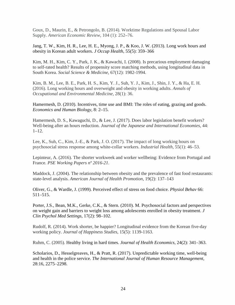
Table 6. Gender Heterogeneous Effects
All Blue collars White collars
Panel A. Dependent variable = Body Mass Index (Treated)*(2001-2002) 0.095 0.156* 0.165
(0.321) (0.086) (0.807) (Treated)*(1999-2000) 0.006 0.062 -0.033
(0.215) (0.069) (0.435) (Treated)*(2003-2006) -0.587 -1.399** 0.175
(0.711) (0.604) (0.992) (Treated)*(2001-2002)*female -0.047 0.108 -0.11
(0.095) (0.255) (0.133) (Treated)*(1999-2000)*female -0.009 0.058 -0.124
(0.06) (0.121) (0.084) (Treated)*(2003-2006)*female 0.007 0.212 -0.108
(0.157) (0.32) (0.179) R2 0.12 0.1 0.12 Panel B. Dependent variable = Overweight (Treated)*(2001-2002) 0.02 0.076*** -0.036
(0.015) (0.02) (0.044) (Treated)*(1999-2000) 0.005 0.012 -0.005
(0.029) (0.021) (0.047) (Treated)*(2003-2006) -0.043 -0.064 -0.02
(0.069) (0.056) (0.099) (Treated)*(2001-2002)*female 0.007 0.017 0.014
(0.011) (0.026) (0.015) (Treated)*(1999-2000)*female -0.005 0.008 -0.016
(0.009) (0.014) (0.011) (Treated)*(2003-2006)*female 0.007 0.036 -0.005
(0.022) (0.037) (0.024) R2 0.11 0.08 0.12 N 49,830 23,297 26,533 Year fixed effects yes yes yes Department fixed effect yes yes yes Controls yes yes yes Note: Body Mass Index = weight/(height^2); estimated with self-reported information of weight and height. Only respondents who worked during reference period. OLS, standard errors (in parenthesis) clustered at department level. * p<0.1; ** p<0.05; *** p<0.01. Controls include demographics (age, age squared, gender), and educational attainment. Full values of estimates are included in the appendix.

33
Table 7. Children Specific Heterogeneous Effects All Blue collars White collars Panel A. Dependent variable = Body Mass Index (Treated)*(2001-2002) 0.061 0.157 0.104 (0.372) (0.228) (0.819) (Treated)*(1999-2000) -0.006 0.254 -0.411 (0.354) (0.167) (0.686) (Treated)*(2003-2006) -0.527 -0.994 0.049 (0.773) (0.902) (0.917) (Treated)*(2001-2002)*haschild 0.248** 0.165 0.287 (0.12) (0.171) (0.191) (Treated)*(1999-2000)*haschild 0.235*** 0.182* 0.301* (0.08) (0.103) (0.152) (Treated)*(2003-2006)*haschild 0.208 -0.006 0.305 (0.188) (0.283) (0.246) Haschild -0.214*** -0.164* -0.253* (0.08) (0.09) (0.142) R2 0.12 0.10 0.12 Panel B. Dependent variable = Overweight (Treated)*(2001-2002) -0.005 0.051 -0.068 (0.027) (0.035) (0.05) (Treated)*(1999-2000) -0.002 0.033 -0.065 (0.042) (0.028) (0.073) (Treated)*(2003-2006) -0.019 -0.001 -0.036 (0.063) (0.075) (0.108) (Treated)*(2001-2002)*haschild 0.034* 0.044** 0.024 (0.02) (0.022) (0.031) (Treated)*(1999-2000)*haschild 0.018 0.023 0.014 (0.015) (0.019) (0.021) (Treated)*(2003-2006)*haschild 0.032 0.037 0.026 (0.026) (0.033) (0.035) Haschild -0.037*** -0.040** -0.032* (0.012) (0.016) (0.019) R2 0.11 0.08 0.12 N 36,249 17,207 19,042 Year fixed effects yes yes yes Department fixed effect yes yes yes Controls yes yes yes

34
Note: Body Mass Index = weight/(height^2); estimated with self-reported information of weight and height. Overweight = 1 if the body mass index is 25 or more. Only respondents who worked during reference period. OLS, standard errors (in parenthesis) clustered at department level. * p<0.1; ** p<0.05; *** p<0.01. Controls include demographics (age, age squared, gender), and educational attainment. Full values of estimates are included in the appendix.

35
Table 8. Effects on health and health related behaviours
All Blue collars White collars Panel A. Dependent variable = Self-assessed health [Very good=1, Very poor=8] (Treated)*(2001-2002) -0.089* -0.104 -0.048 (0.047) (0.09) (0.038) (Treated)*(1999-2000) -0.018 -0.026 -0.004 (0.049) (0.039) (0.078) (Treated)*(2003-2006) 0.201 0.247 0.182 (0.141) (0.189) (0.149) R2 0.02 0.03 0.03 N 49,641 23,214 26,427 Panel B. Dependent variable = Self-assessed health [Good =1, Suboptimum=0] (Treated)*(2001-2002) 0.014 0.027 -0.009 (0.015) (0.017) (0.012) (Treated)*(1999-2000) 0.014 0.009 0.021 (0.021) (0.014) (0.032) (Treated)*(2003-2006) -0.026 -0.058 -0.006 (0.05) (0.058) (0.067) N 49,619 23,209 26,401 Panel C. Dependent variable = Smokes [Yes=1, No=0] (Treated)*(2001-2002) -0.001 -0.005 -0.000 (0.015) (0.01) (0.036) (Treated)*(1999-2000) 0.032*** 0.019** 0.045** (0.007) (0.008) (0.02) (Treated)*(after 2002) -0.041 -0.053 -0.042 (0.052) (0.043) (0.055) N 48,713 22,785 25,841 Panel D. Dependent variable = Cigarettes smoked for those who smoke (Treated)*(2001-2002) 0.928 -1.856 1.996 (1.735) (1.574) (2.907) (Treated)*(1999-2000) 0.814 0.88 1.326 (1.326) (0.616) (2.286) (Treated)*(2003-2006) 2.451 10.845*** -0.908 (1.674) (2.141) (3.082) R2 0.06 0.12 0.1 N 6,428 2,954 3,474 Year fixed effects yes yes yes

36
Department fixed effect yes yes yes Controls yes yes yes
Note: Only respondents who worked during reference period. Panel A and D = OLS estimates; Panel B and C = Probit estimates (marginal effect showed). Standard errors (in parenthesis) clustered at department level. * p<0.1; ** p<0.05; *** p<0.01. Controls include demographics (age, age squared, gender), and educational attainment. Full values of estimates are included in the appendix.

37
Table 9. Placebo test using other regions as control groups (effects on overweight) All Blue collars White collars (Treated_IledeFrance)*(2001-2002) -0.006 -0.027 0.004 (0.013) (0.021) (0.018) (Treated_IledeFrance)*(1999-2000) -0.01 -0.026* 0.005 (0.006) (0.014) (0.011) (Treated_IledeFrance)*(2003-2006) -0.026 -0.053** -0.012 (0.021) (0.026) (0.023) R2 0.11 0.08 0.12 (Treated_Auvergne)*(2001-2002) 0.011 -0.022 0.039** (0.022) (0.064) (0.018) (Treated_Auvergne)*(1999-2000) 0.007 0.018 0.004 (0.011) (0.027) (0.012) (Treated_Auvergne)*(2003-2006) 0.021 -0.068 0.070*** (0.05) (0.112) (0.027) R2 0.11 0.08 0.12 N 49,830 23,297 26,533 Note: Body Mass Index = weight/(height^2); estimated with self-reported information of weight and height. Overweight = 1 if the body mass index is 25 or more. Only respondents who worked during reference period. OLS, standard errors (in parenthesis) clustered at department level. * p<0.1; ** p<0.05; *** p<0.01. Controls include demographics (age, age squared, gender), and educational attainment. Full values of estimates are included in the appendix.

38
Figures 1. Trends in Overweight and Body Mass Index, 1997-2006
Note: Body Mass Index = weight/(height^2); estimated with self-reported information of weight and height. Overweight = 1 if the body mass index is 25 or more. Only respondents who worked during reference period.

39
Appendix Figure A0. Regions of France
Note: In 2014, the French Parliament approved an initiative that reduced the number of regions from 22 to 13; the map shows the existing 22 regions during the Aubry reform.
40
Figure A1. Trends in Obesity, 1997-2006
Note: Body Mass Index = weight/(height^2); estimated with self-reported information of weight and height. Obesity = 1 if the body mass index is 30 or more. Only respondents who worked during reference period.

41
Table A1. Number of Observations by Year Year Frequency % 1997 10,505 21.1 1998 9,370 18.8 1999 7,982 16.0 2000 6,141 12.3 2001 5,045 10.1 2002 3,438 6.9 2003 2,518 5.1 2004 1,935 3.9 2005 1,574 3.2 2006 1,322 2.7 Total 49,830 100.0 Note: The sample include only respondents who work during reference period (1997-2006), with complete information. Territories are excluded. Unbalanced panel: 11,607 individuals; 49,830 observations.
42
Table A2. Effect of Working Time Reduction on Overweight, 1997-2006 Probit Estimates (marginal effects)
All Blue collars White collars (Treated)*(2001-2002) 0.027* 0.084*** -0.029 (0.015) (0.022) (0.048) (Treated)*(1999-2000) 0.004 0.014 -0.012 (0.033) (0.022) (0.053) (Treated)*(2003-2006) -0.042 -0.064 -0.021 (0.075) (0.069) (0.105) Controls Yes Yes Yes Year fixed effects Yes Yes Yes Department fixed effect Yes Yes Yes N 49,830 23,297 26,533
Note: Body Mass Index = weight/(height^2); estimated with self-reported information of weight and height. Overweight = 1 if the body mass index is 25 or more. Only respondents who worked during reference period. Standard errors (in parenthesis) clustered at department level. * p<0.1; ** p<0.05; *** p<0.01. Controls include demographics (age, age squared, gender), and educational attainment.

43
Table A3. Effect of Working Time Reduction on Obesity, 1997-2006 All Blue collars White collars
Panel A. OLS, no controls (Treated)*(2001-2002) 0.005 -0.020 0.047 (0.016) (0.012) (0.044) (Treated)*(1999-2000) -0.010 -0.016 -0.000 (0.008) (0.013) (0.035) (Treated)*(2003-2006) -0.054 -0.200*** 0.061 (0.036) (0.041) (0.053) R2 0.01 0.02 0.02 Panel B. OLS, with controls (Treated)*(2001-2002) 0.007 -0.017 0.044 (0.016) (0.013) (0.047) (Treated)*(1999-2000) -0.010 -0.015 -0.003 (0.008) (0.014) (0.036) (Treated)*( 2003-2006) -0.056 -0.194*** 0.057 (0.038) (0.039) (0.056) R2 0.02 0.03 0.02
Panel C. Probit estimates (marginal effects), with controls (Treated)*(2001-2002) 0.008 -0.011 0.038 (0.014) (0.010) (0.046) (Treated)*(1999-2000) -0.006 -0.010 -0.000 (0.007) (0.010) (0.023) (Treated)*( 2003-2006) -0.033* -0.080*** 0.050 (0.019) (0.007) (0.062) N 49,830 23,297 26,533
Note: Body Mass Index = weight/(height^2); estimated with self-reported information of weight and height. Obesity = 1 if the body mass index is 30 or more. Only respondents who worked during reference period. Standard errors (in parenthesis) clustered at department level. * p<0.1; ** p<0.05; *** p<0.01. Controls include demographics (age, age squared, gender), and educational attainment.

44
Table B1. Effect of Treatment on Body Mass Index, 1997-2006 All Blue collars White collars (Treated)*(2001-2002) 0.077 0.170** 0.104 (0.321) (0.084) (0.819) (Treated)*(1999-2000) 0.003 0.070 -0.092 (0.213) (0.062) (0.441) (Treated)*(2003-2006) -0.584 -1.338** 0.095 (0.709) (0.589) (1.003) Female -2.296*** -2.270*** -2.152*** (0.103) (0.155) (0.133) Age 1.149*** 1.118*** 1.200*** (0.166) (0.303) (0.223) Age2 -0.011*** -0.010*** -0.011*** (0.002) (0.003) (0.002) Junior secondary certificate -1.078*** -1.051*** -1.088*** (0.259) (0.278) (0.405) Baccalaureate -0.987*** -1.032*** -0.952** (0.272) (0.324) (0.414) Professional competence -0.837*** -0.721*** -1.013** (0.242) (0.263) (0.424) Vocational certificate -1.082*** -0.980*** -1.156*** (0.264) (0.300) (0.424) Undergraduate degree -1.224*** -1.325*** -1.126** (0.305) (0.314) (0.502) Other academic degree -1.401*** -1.292*** -1.399*** (0.247) (0.260) (0.401) Other diploma -1.178*** -0.764** -1.477*** (0.317) (0.336) (0.470) Year fixed effects yes yes yes Department fixed effect yes yes yes Constant -4.371 -3.983 -5.454 (4.432) (8.076) (5.974) R2 0.12 0.10 0.12 N 49,830 23,297 26,533
Note: Body Mass Index = weight/(height^2); estimated with self-reported information of weight and height. Only respondents who worked during reference period. OLS, standard errors (in parenthesis) clustered at department level. * p<0.1; ** p<0.05; *** p<0.01.

45
Table B2. Effect of Treatment on Overweight, 1997-2006 All Blue collars White collars (Treated)*(2001-2002) 0.023* 0.078*** -0.029 (0.014) (0.019) (0.044) (Treated)*(1999-2000) 0.003 0.013 -0.012 (0.029) (0.020) (0.048) (Treated)*(2003-2006) -0.040 -0.054 -0.023 (0.068) (0.054) (0.100) Female -0.324*** -0.308*** -0.310*** (0.011) (0.021) (0.013) Age 0.140*** 0.125*** 0.151*** (0.022) (0.040) (0.025) Age2 -0.001*** -0.001*** -0.001*** (0.000) (0.000) (0.000) Junior secondary certificate -0.098*** -0.076** -0.124*** (0.028) (0.032) (0.038) Baccalaureate -0.102*** -0.091** -0.119*** (0.026) (0.040) (0.036) Professional competence -0.073*** -0.044 -0.111*** (0.024) (0.030) (0.037) Vocational certificate -0.093*** -0.059* -0.129*** (0.027) (0.033) (0.040) Undergraduate degree -0.113*** -0.118*** -0.113** (0.032) (0.036) (0.051) Other academic degree -0.145*** -0.110*** -0.168*** (0.025) (0.032) (0.039) Other diploma -0.108** -0.069 -0.140*** (0.042) (0.050) (0.051) Year fixed effects yes yes yes Department fixed effect yes yes yes Constant -3.040*** -2.717** -3.305*** (0.599) (1.083) (0.670) R2 0.11 0.08 0.12 N 49,830 23,297 26,533
Body Mass Index = weight/(height^2); estimated with self-reported information of weight and height. Overweight = 1 if the body mass index is 25 or more. Only respondents who worked during reference period. OLS, standard errors (in parenthesis) clustered at department level. * p<0.1; ** p<0.05; *** p<0.01.

46
Table B3. Effect of Treatment on Obesity, 1997-2006 All Blue collars White collars (Treated)*(2001-2002) 0.007 -0.017 0.044 (0.016) (0.013) (0.047) (Treated)*(1999-2000) -0.010 -0.015 -0.003 (0.008) (0.014) (0.036) (Treated)*(2003-2006) -0.056 -0.194*** 0.057 (0.038) (0.039) (0.056) Female -0.031*** -0.036*** -0.021** (0.008) (0.011) (0.010) Age 0.031** 0.025 0.035** (0.013) (0.024) (0.015) Age2 -0.000** -0.000 -0.000** (0.000) (0.000) (0.000) Junior secondary certificate -0.089*** -0.101*** -0.070** (0.018) (0.026) (0.031) Baccalaureate -0.062*** -0.083*** -0.039 (0.017) (0.025) (0.030) Professional competence -0.066*** -0.073*** -0.059* (0.018) (0.024) (0.033) Vocational certificate -0.084*** -0.095*** -0.068** (0.017) (0.026) (0.031) Undergraduate degree -0.085*** -0.100*** -0.069** (0.021) (0.028) (0.034) Other academic degree -0.088*** -0.106*** -0.064** (0.017) (0.024) (0.028) Other diploma -0.089*** -0.059* -0.108*** (0.023) (0.032) (0.037) Year fixed effects yes yes yes Department fixed effect yes yes yes Constant -0.693** -0.610 -0.776* (0.330) (0.614) (0.403) R2 0.02 0.03 0.02 N 49,830 23,297 26,533
Body Mass Index = weight/(height^2); estimated with self-reported information of weight and height. Obesity = 1 if the body mass index is 30 or more. Only respondents who worked during reference period. OLS, standard errors (in parenthesis) clustered at department level. * p<0.1; ** p<0.05; *** p<0.01.

47
Table B4. Alternative Specification without Pre-treatment Trends, BMI All Blue collars White collars (Treated)*(2001-2002) 0.076 0.142 0.142 (0.243) (0.091) (0.664) (Treated)*(2003-2006) -0.585 -1.366** 0.132 (0.626) (0.570) (0.832) Female -2.296*** -2.270*** -2.152*** (0.103) (0.155) (0.133) Age 1.149*** 1.118*** 1.200*** (0.166) (0.303) (0.223) Age2 -0.011*** -0.010*** -0.011*** (0.002) (0.003) (0.002) Junior secondary certificate -1.078*** -1.051*** -1.088*** (0.259) (0.278) (0.405) Baccalaureate -0.987*** -1.032*** -0.952** (0.272) (0.324) (0.414) Professional competence -0.837*** -0.721*** -1.013** (0.242) (0.263) (0.424) Vocational certificate -1.082*** -0.979*** -1.156*** (0.264) (0.300) (0.424) Undergraduate degree -1.224*** -1.325*** -1.125** (0.305) (0.314) (0.502) Other academic degree -1.401*** -1.292*** -1.399*** (0.247) (0.260) (0.401) Other diploma -1.178*** -0.764** -1.477*** (0.317) (0.336) (0.470) Year fixed effects yes yes yes Department fixed effect yes yes yes Constant -4.371 -3.978 -5.456 (4.432) (8.076) (5.974) R2 0.12 0.10 0.12 N 49,830 23,297 26,533
Body Mass Index = weight/(height^2); estimated with self-reported information of weight and height. Only respondents who worked during reference period. OLS, standard errors (in parenthesis) clustered at department level. * p<0.1; ** p<0.05; *** p<0.01.

48
Table B5. Alternative Specification without Pre-treatment Trends, Overweight All Blue collars White collars (Treated)*(2001-2002) 0.022*** 0.073*** -0.024 (0.008) (0.020) (0.025) (Treated)*(2003-2006) -0.041 -0.059 -0.018 (0.056) (0.047) (0.081) Female -0.324*** -0.308*** -0.310*** (0.011) (0.021) (0.013) Age 0.140*** 0.125*** 0.151*** (0.022) (0.040) (0.025) Age2 -0.001*** -0.001*** -0.001*** (0.000) (0.000) (0.000) Junior secondary certificate -0.098*** -0.076** -0.123*** (0.028) (0.032) (0.038) Baccalaureate -0.102*** -0.091** -0.119*** (0.026) (0.040) (0.036) Professional competence -0.073*** -0.044 -0.111*** (0.024) (0.030) (0.037) Vocational certificate -0.093*** -0.059* -0.129*** (0.027) (0.033) (0.040) Undergraduate degree -0.113*** -0.118*** -0.113** (0.032) (0.036) (0.052) Other academic degree -0.145*** -0.110*** -0.168*** (0.025) (0.032) (0.039) Other diploma -0.108** -0.069 -0.140*** (0.042) (0.050) (0.051) Year fixed effects yes yes yes Department fixed effect yes yes yes Constant -3.040*** -2.716** -3.305*** (0.599) (1.083) (0.670) R2 0.11 0.08 0.12 N 49,830 23,297 26,533
Body Mass Index = weight/(height^2); estimated with self-reported information of weight and height. Overweight = 1 if the body mass index is 25 or more. Only respondents who worked during reference period. OLS, standard errors (in parenthesis) clustered at department level. * p<0.1; ** p<0.05; *** p<0.01.

49
Table C1. Effect of Treatment on BMI, additional control for activity sector All Blue collars White collars (Treated)*(2001-2002) 0.075 0.171** 0.100 (0.320) (0.086) (0.819) (Treated)*(1999-2000) 0.001 0.069 -0.095 (0.214) (0.061) (0.442) (Treated)*(after 2002) -0.584 -1.336** 0.094 (0.705) (0.580) (1.002) Female -2.297*** -2.268*** -2.153*** (0.104) (0.154) (0.133) Age 1.149*** 1.116*** 1.201*** (0.166) (0.304) (0.223) Age2 -0.011*** -0.010*** -0.011*** (0.002) (0.003) (0.002) Junior secondary certificate -1.078*** -1.051*** -1.088*** (0.259) (0.277) (0.404) Baccalaureate -0.985*** -1.028*** -0.950** (0.271) (0.325) (0.412) Professional competence -0.837*** -0.722*** -1.013** (0.242) (0.263) (0.424) Vocational certificate -1.081*** -0.977*** -1.155*** (0.263) (0.299) (0.422) Undergraduate degree -1.219*** -1.315*** -1.122** (0.303) (0.314) (0.500) Other academic degree -1.395*** -1.284*** -1.392*** (0.246) (0.261) (0.397) Other diploma -1.175*** -0.758** -1.474*** (0.317) (0.334) (0.468) Distribution 0.033 0.046 0.031 (0.071) (0.120) (0.092) Year fixed effects yes yes Yes Department fixed effect yes yes Yes Constant -4.380 -3.936 -5.484 (4.428) (8.091) (5.966) R2 0.12 0.10 0.12 N 49,830 23,297 26,533
Body Mass Index = weight/(height^2); estimated with self-reported information of weight and height. Only respondents who worked during reference period. OLS, standard errors (in parenthesis) clustered at department level. * p<0.1; ** p<0.05; *** p<0.01.
50
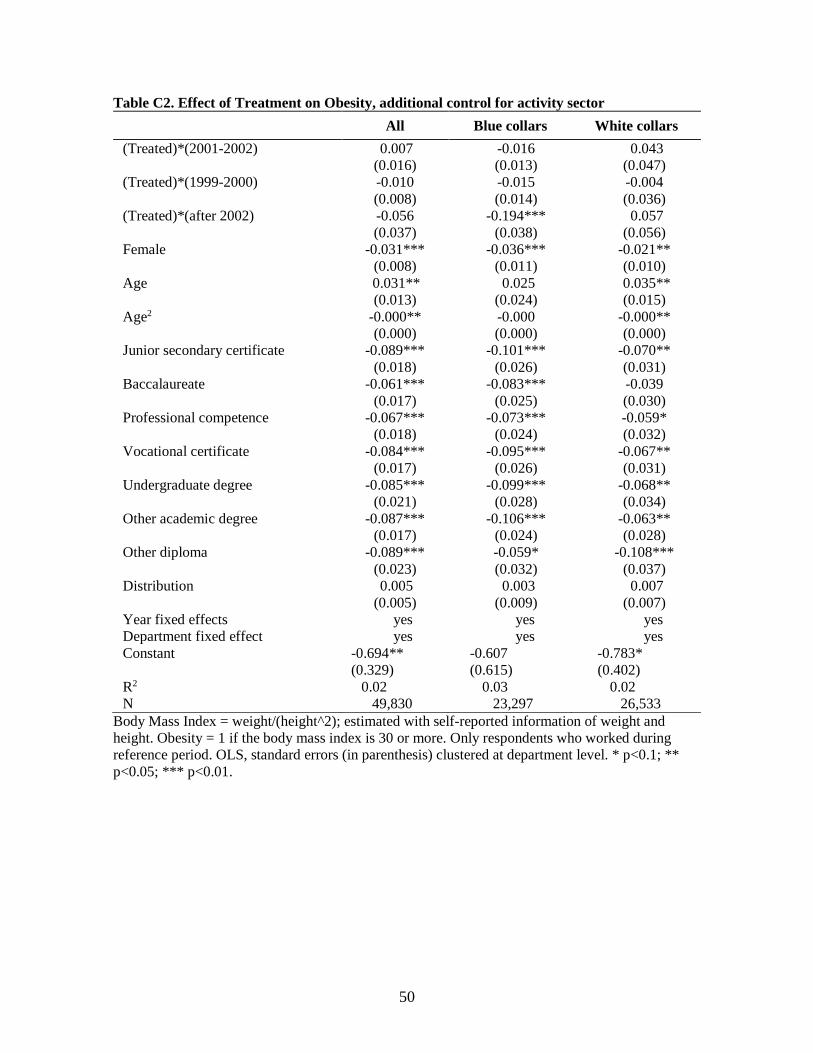
Table C2. Effect of Treatment on Obesity, additional control for activity sector All Blue collars White collars (Treated)*(2001-2002) 0.007 -0.016 0.043 (0.016) (0.013) (0.047) (Treated)*(1999-2000) -0.010 -0.015 -0.004 (0.008) (0.014) (0.036) (Treated)*(after 2002) -0.056 -0.194*** 0.057 (0.037) (0.038) (0.056) Female -0.031*** -0.036*** -0.021** (0.008) (0.011) (0.010) Age 0.031** 0.025 0.035** (0.013) (0.024) (0.015) Age2 -0.000** -0.000 -0.000** (0.000) (0.000) (0.000) Junior secondary certificate -0.089*** -0.101*** -0.070** (0.018) (0.026) (0.031) Baccalaureate -0.061*** -0.083*** -0.039 (0.017) (0.025) (0.030) Professional competence -0.067*** -0.073*** -0.059* (0.018) (0.024) (0.032) Vocational certificate -0.084*** -0.095*** -0.067** (0.017) (0.026) (0.031) Undergraduate degree -0.085*** -0.099*** -0.068** (0.021) (0.028) (0.034) Other academic degree -0.087*** -0.106*** -0.063** (0.017) (0.024) (0.028) Other diploma -0.089*** -0.059* -0.108*** (0.023) (0.032) (0.037) Distribution 0.005 0.003 0.007 (0.005) (0.009) (0.007) Year fixed effects yes yes yes Department fixed effect yes yes yes Constant -0.694** -0.607 -0.783* (0.329) (0.615) (0.402) R2 0.02 0.03 0.02 N 49,830 23,297 26,533
Body Mass Index = weight/(height^2); estimated with self-reported information of weight and height. Obesity = 1 if the body mass index is 30 or more. Only respondents who worked during reference period. OLS, standard errors (in parenthesis) clustered at department level. * p<0.1; ** p<0.05; *** p<0.01.

51
Table C3. Effect of Treatment on Overweight, additional control for activity sector
All Blue collars White collars (Treated)*(2001-2002) 0.023* 0.078*** -0.028 (0.014) (0.019) (0.045) (Treated)*(1999-2000) 0.003 0.013 -0.012 (0.029) (0.020) (0.048) (Treated)*(after 2002) -0.040 -0.054 -0.023 (0.068) (0.054) (0.100) Female -0.323*** -0.308*** -0.310*** (0.011) (0.020) (0.013) Age 0.140*** 0.125*** 0.151*** (0.022) (0.040) (0.025) Age2 -0.001*** -0.001*** -0.001*** (0.000) (0.000) (0.000) Junior secondary certificate -0.098*** -0.076** -0.123*** (0.028) (0.032) (0.038) Baccalaureate -0.102*** -0.091** -0.119*** (0.025) (0.040) (0.036) Professional competence -0.072*** -0.044 -0.111*** (0.024) (0.030) (0.037) Vocational certificate -0.093*** -0.059* -0.129*** (0.027) (0.033) (0.040) Undergraduate degree -0.114*** -0.118*** -0.114** (0.032) (0.036) (0.051) Other academic degree -0.145*** -0.110*** -0.169*** (0.025) (0.032) (0.038) Other diploma -0.108** -0.069 -0.140*** (0.042) (0.049) (0.051) Distribution -0.003 0.000 -0.003 (0.010) (0.015) (0.013) Year fixed effects yes yes Yes Department fixed effect yes yes Yes Constant -3.039*** -2.717** -3.302*** (0.598) (1.086) (0.667) R2 0.11 0.08 0.12 N 49,830 23,297 26,533
Body Mass Index = weight/(height^2); estimated with self-reported information of weight and height. Overweight = 1 if the body mass index is 25 or more. Only respondents who worked during reference period. OLS, standard errors (in parenthesis) clustered at department level. * p<0.1; ** p<0.05; *** p<0.01.

52
Table C4. Effect of Treatment on BMI, additional controls for spousal employment status and household income
All Blue collars White collars (Treated)*(2001-2002) 0.190 0.200* 0.321 (0.331) (0.105) (0.811) (Treated)*(1999-2000) -0.023 0.093 -0.228 (0.193) (0.080) (0.395) (Treated)*(after 2002) -0.616 -1.403* 0.142 (0.860) (0.746) (1.030) Female -2.133*** -2.134*** -1.992*** (0.120) (0.169) (0.148) Age 1.207*** 1.126*** 1.280*** (0.197) (0.320) (0.222) Age2 -0.011*** -0.010*** -0.011*** (0.002) (0.003) (0.002) Junior secondary certificate -1.122*** -0.979*** -1.297** (0.288) (0.266) (0.525) Baccalaureate -0.892*** -0.869*** -0.992* (0.308) (0.326) (0.548) Professional competence -0.793*** -0.622** -1.075** (0.263) (0.259) (0.525) Vocational certificate -1.071*** -0.861*** -1.331** (0.276) (0.277) (0.531) Undergraduate degree -1.077*** -1.163*** -1.084* (0.322) (0.303) (0.608) Other academic degree -1.316*** -1.148*** -1.461*** (0.256) (0.256) (0.463) Other diploma -1.103*** -0.636* -1.557*** (0.327) (0.329) (0.558) Middle income -0.145 -0.105 -0.160 (0.116) (0.127) (0.196) High income -0.456*** -0.333** -0.527*** (0.135) (0.157) (0.200) Spouse works -0.267*** -0.244*** -0.278*** (0.063) (0.092) (0.090) Year fixed effects yes yes Yes Department fixed effect yes yes Yes Constant -5.990 -3.785 -7.909 (5.281) (8.531) (6.136) R2 0.12 0.09 0.13 N 41,449 20,173 21,276
Body Mass Index = weight/(height^2); estimated with self-reported information of weight and height. Only respondents who worked during reference period. OLS, standard errors (in parenthesis) clustered at department level. * p<0.1; ** p<0.05; *** p<0.01.

53
Table C5. Effect of Treatment on Obesity, additional controls for spousal employment status and household income
All Blue collars White collars (Treated)*(2001-2002) 0.016 -0.010 0.056 (0.010) (0.025) (0.055) (Treated)*(1999-2000) -0.007 -0.008 -0.007 (0.006) (0.023) (0.023) (Treated)*(after 2002) -0.071* -0.213*** 0.054 (0.041) (0.024) (0.050) Female -0.025** -0.030** -0.018* (0.010) (0.013) (0.011) Age 0.041** 0.026 0.050*** (0.015) (0.027) (0.016) Age2 -0.000** -0.000 -0.000*** (0.000) (0.000) (0.000) Junior secondary certificate -0.098*** -0.095*** -0.099*** (0.021) (0.026) (0.037) Baccalaureate -0.065*** -0.072*** -0.062 (0.021) (0.024) (0.039) Professional competence -0.071*** -0.067** -0.079** (0.020) (0.026) (0.038) Vocational certificate -0.089*** -0.085*** -0.093** (0.018) (0.026) (0.037) Undergraduate degree -0.080*** -0.086*** -0.080** (0.022) (0.029) (0.039) Other academic degree -0.089*** -0.099*** -0.084** (0.020) (0.029) (0.032) Other diploma -0.085*** -0.045 -0.124*** (0.026) (0.036) (0.041) Middle income -0.020** -0.026** -0.008 (0.009) (0.012) (0.013) High income -0.040*** -0.033** -0.036** (0.010) (0.014) (0.015) Spouse works -0.018*** -0.017** -0.017** (0.006) (0.008) (0.007) Year fixed effects yes yes Yes Department fixed effect yes yes Yes Constant -0.930** -0.587 -1.126*** (0.395) (0.699) (0.427) R2 0.02 0.03 0.03 N 41,449 20,173 21,276
Body Mass Index = weight/(height^2); estimated with self-reported information of weight and height. Obesity = 1 if the body mass index is 30 or more. Only respondents who worked during reference period. OLS, standard errors (in parenthesis) clustered at department level. * p<0.1; ** p<0.05; *** p<0.01.

54
Table C6. Effect of Treatment on Overweight, additional controls for spousal employment status and household income
All Blue collars White collars (Treated)*(2001-2002) 0.026 0.082*** -0.030 (0.019) (0.022) (0.042) (Treated)*(1999-2000) -0.006 0.013 -0.038 (0.032) (0.029) (0.046) (Treated)*(after 2002) -0.032 -0.057 -0.005 (0.080) (0.073) (0.103) Female -0.311*** -0.297*** -0.295*** (0.013) (0.022) (0.016) Age 0.142*** 0.109** 0.162*** (0.028) (0.046) (0.029) Age2 -0.001*** -0.001** -0.001*** (0.000) (0.000) (0.000) Junior secondary certificate -0.100*** -0.069** -0.143*** (0.032) (0.034) (0.053) Baccalaureate -0.098*** -0.095** -0.121** (0.031) (0.041) (0.050) Professional competence -0.069** -0.038 -0.117** (0.027) (0.032) (0.051) Vocational certificate -0.097*** -0.059* -0.152*** (0.028) (0.033) (0.050) Undergraduate degree -0.107*** -0.120*** -0.110* (0.035) (0.040) (0.063) Other academic degree -0.138*** -0.105*** -0.173*** (0.029) (0.035) (0.047) Other diploma -0.110** -0.071 -0.152** (0.046) (0.051) (0.065) Middle income -0.005 0.011 -0.027 (0.016) (0.017) (0.025) High income -0.030* -0.009 -0.053** (0.017) (0.018) (0.025) Spouse works -0.028*** -0.025** -0.031** (0.009) (0.013) (0.013) Year fixed effects yes yes Yes Department fixed effect yes yes Yes Constant -3.097*** -2.237* -3.603*** (0.748) (1.234) (0.782) R2 0.11 0.07 0.12 N 41,449 20,173 21,276
Body Mass Index = weight/(height^2); estimated with self-reported information of weight and height. Overweight = 1 if the body mass index is 25 or more. Only respondents who worked during reference period. OLS, standard errors (in parenthesis) clustered at department level. * p<0.1; ** p<0.05; *** p<0.01.

55
Table D1. Effect of Treatment on BMI by area of activity Distribution Production
All Blue collars White collars All Blue collars White collars (Treated)*(2001-2002) -0.279 0.127 -0.915 0.433 0.321*** 0.616 (0.392) (0.161) (0.713) (0.368) (0.116) (0.833) (Treated)*(1999-2000) -0.133 0.198 -0.654 0.200 0.117 0.304 (0.372) (0.158) (0.540) (0.179) (0.075) (0.394) (Treated)*(2003-2006) -1.842** -2.978*** -0.661 0.348 0.095 0.612 (0.792) (0.436) (1.281) (0.537) (0.376) (0.865) Female -2.257*** -2.056*** -2.133*** -2.348*** -2.498*** -2.188*** (0.125) (0.221) (0.143) (0.140) (0.153) (0.207) Age 1.167*** 0.945* 1.205*** 1.177*** 1.199*** 1.191*** (0.250) (0.479) (0.315) (0.204) (0.346) (0.285) Age2 -0.011*** -0.008* -0.011*** -0.011*** -0.011*** -0.011*** (0.002) (0.005) (0.003) (0.002) (0.003) (0.003) Junior sec certificate -1.051*** -0.792** -1.282** -1.139*** -1.556*** -0.763 (0.282) (0.336) (0.493) (0.404) (0.422) (0.611) Baccalaureate -0.849*** -0.709* -1.004* -1.119** -1.397*** -0.817 (0.302) (0.381) (0.527) (0.454) (0.528) (0.653) Prof competence -0.775*** -0.630* -1.035** -0.924** -0.840* -1.010* (0.264) (0.319) (0.520) (0.396) (0.424) (0.587) Vocational certificate -0.905*** -0.780** -1.051** -1.309*** -1.242*** -1.269** (0.268) (0.335) (0.517) (0.419) (0.454) (0.600) Undergraduate degree -0.954*** -1.057** -0.943* -1.469*** -1.666*** -1.265* (0.321) (0.411) (0.546) (0.436) (0.417) (0.730) Other academic degree -1.174*** -1.037*** -1.225** -1.560*** -1.527*** -1.415** (0.298) (0.374) (0.509) (0.402) (0.443) (0.589) Other diploma -0.785* -0.194 -1.181* -1.509*** -1.215*** -1.643** (0.452) (0.490) (0.634) (0.369) (0.406) (0.639) Constant -4.796 0.061 -5.350 -5.038 -5.273 -5.541 (6.565) (12.484) (8.281) (5.474) (9.398) (7.723) R2 0.12 0.09 0.14 0.13 0.16 0.12 N 25,471 11,889 13,582 24,359 11,408 12,951

56
Body Mass Index = weight/(height^2); estimated with self-reported information of weight and height. Only respondents who worked during reference period. OLS, standard errors (in parenthesis) clustered at department level. * p<0.1; ** p<0.05; *** p<0.01. Table D2. Effect of Treatment on Overweight by area of activity
Distribution Production
All Blue collars White collars All Blue collars White collars (Treated)*(2001-2002) -0.009 0.088*** -0.194*** 0.063** 0.090*** 0.045 (0.021) (0.027) (0.056) (0.026) (0.025) (0.037) (Treated)*(1999-2000) -0.017 0.018 -0.071 0.029 0.022 0.027 (0.060) (0.020) (0.109) (0.023) (0.028) (0.018) (Treated)*(2003-2006) -0.152 -0.165*** -0.117 0.052 0.051 0.035 (0.109) (0.059) (0.184) (0.048) (0.052) (0.054) Female -0.319*** -0.282*** -0.307*** -0.329*** -0.338*** -0.316*** (0.015) (0.029) (0.019) (0.014) (0.027) (0.017) Age 0.158*** 0.167*** 0.146*** 0.126*** 0.086* 0.153*** (0.029) (0.059) (0.034) (0.031) (0.048) (0.038) Age2 -0.001*** -0.002*** -0.001*** -0.001*** -0.001* -0.001*** (0.000) (0.001) (0.000) (0.000) (0.000) (0.000) Junior sec certificate -0.069** -0.027 -0.110** -0.138*** -0.143*** -0.145** (0.030) (0.042) (0.044) (0.040) (0.042) (0.064) Baccalaureate -0.076*** -0.048 -0.100** -0.131*** -0.132** -0.143** (0.025) (0.046) (0.042) (0.044) (0.061) (0.067) Prof competence -0.057** -0.037 -0.090** -0.092** -0.047 -0.148** (0.025) (0.040) (0.044) (0.041) (0.044) (0.061) Vocational certificate -0.059** -0.042 -0.082* -0.137*** -0.080* -0.198*** (0.024) (0.039) (0.044) (0.044) (0.046) (0.066) Undergraduate degree -0.084** -0.092* -0.082 -0.146*** -0.147*** -0.155* (0.033) (0.052) (0.052) (0.050) (0.043) (0.086) Other academic degree -0.108*** -0.069 -0.131*** -0.181*** -0.152*** -0.208*** (0.029) (0.048) (0.048) (0.040) (0.049) (0.063) Other diploma -0.035 0.033 -0.087 -0.174*** -0.154*** -0.192** (0.060) (0.069) (0.070) (0.053) (0.058) (0.078)

57
Constant -3.542*** -3.925** -3.194*** -2.661*** -1.561 -3.354*** (0.748) (1.537) (0.873) (0.833) (1.318) (1.022) R2 0.12 0.08 0.13 0.12 0.11 0.13 N 25,471 11,889 13,582 24,359 11,408 12,951
Body Mass Index = weight/(height^2); estimated with self-reported information of weight and height. Overweight = 1 if the body mass index is 25 or more. Only respondents who worked during reference period. OLS, standard errors (in parenthesis) clustered at department level. * p<0.1; ** p<0.05; *** p<0.01.

58
Table E1. Effect of Treatment on BMI, income interactions All Blue collars White collars (Treated)*(2001-2002) -0.050 0.076 -0.079 (0.341) (0.166) (0.897) (Treated)*(1999-2000) -0.078 0.031 -0.187 (0.222) (0.094) (0.497) (Treated)*(2003-2006) -0.659 -1.383** -0.005 (0.740) (0.636) (1.076) (Treated)*(2001-2002)*middle income 0.108 0.194 -0.008 (0.116) (0.183) (0.186) (Treated)*(2001-2002)*high income 0.137 0.043 0.194 (0.113) (0.223) (0.169) (Treated)*(1999-2000)*middle income 0.025 0.077 -0.085 (0.072) (0.111) (0.134) (Treated)*(1999-2000)* high income 0.107 0.055 0.083 (0.078) (0.122) (0.126) (Treated)*(2003-2006)*middle income 0.068 0.259 -0.127 (0.225) (0.351) (0.303) (Treated)*(2003-2006)*high income 0.058 0.021 0.048 (0.189) (0.381) (0.288) Middle income -0.105 -0.193* 0.110 (0.084) (0.109) (0.157) High income -0.414*** -0.381*** -0.329** (0.104) (0.139) (0.161) Female -2.274*** -2.252*** -2.142*** (0.106) (0.153) (0.142) Age 1.119*** 1.028*** 1.214*** (0.176) (0.307) (0.235) Age2 -0.010*** -0.009*** -0.011*** (0.002) (0.003) (0.002) Junior secondary certificate -1.085*** -1.070*** -1.084** (0.267) (0.291) (0.418) Baccalaureate -0.927*** -0.992*** -0.882** (0.280) (0.323) (0.428) Professional competence -0.841*** -0.747*** -0.988** (0.248) (0.274) (0.436) Vocational certificate -1.077*** -0.980*** -1.147** (0.270) (0.308) (0.437) Undergraduate degree -1.164*** -1.285*** -1.056** (0.308) (0.322) (0.510) Other academic degree -1.244*** -1.139*** -1.254*** (0.250) (0.263) (0.398) Other diploma -1.103*** -0.711** -1.395*** (0.316) (0.333) (0.472) Year fixed effects yes yes Yes Department fixed effect yes yes Yes Constant -2.814 -1.498 -5.921 (4.802) (8.231) (6.479) R2 0.12 0.10 0.12 N 48,873 22,811 26,062
59
Body Mass Index = weight/(height^2); estimated with self-reported information of weight and height. Only respondents who worked during reference period. OLS, standard errors (in parenthesis) clustered at department level. * p<0.1; ** p<0.05; *** p<0.01.

60
Table E2. Effect of Treatment on BMI, spousal employment status interactions All Blue collars White collars (Treated)*(2001-2002) 0.318 0.179 0.651
(0.348) (0.126) (0.845) (Treated)*(1999-2000) 0.089 0.189* -0.045
(0.214) (0.100) (0.434) (Treated)*(2003-2006) -0.433 -1.452* 0.571
(0.860) (0.745) (1.088) (Treated)*(2001-2002)*spouse
works -0.163* 0.008 -0.312**
(0.083) (0.159) (0.149) (Treated)*(1999-2000)*spouse
works -0.135** -0.189** -0.103
(0.064) (0.093) (0.104) (Treated)*(2003-2006)*spouse
works -0.279** -0.042 -0.412**
(0.118) (0.244) (0.177) Spouse works -0.203*** -0.233** -0.136
(0.067) (0.106) (0.098) Female -2.189*** -2.177*** -2.023*** (0.113) (0.170) (0.136) Age 1.272*** 1.172*** 1.356*** (0.189) (0.324) (0.219) Age2 -0.012*** -0.011*** -0.012*** (0.002) (0.003) (0.002) Junior secondary certificate -1.131*** -0.949*** -1.344***
(0.277) (0.256) (0.502) Baccalaureate -0.970*** -0.913*** -1.100**
(0.302) (0.328) (0.536) Professional competence -0.803*** -0.588** -1.161**
(0.258) (0.250) (0.510) Vocational certificate -1.094*** -0.850*** -1.391***
(0.271) (0.271) (0.516) Undergraduate degree -1.168*** -1.185*** -1.228**
(0.319) (0.298) (0.602) Other academic degree -1.512*** -1.279*** -1.692***
(0.256) (0.251) (0.479) Other diploma -1.211*** -0.677** -1.710***
(0.327) (0.329) (0.557) Year fixed effects yes yes Yes Department fixed effect yes yes Yes Constant -7.885 -5.031 -10.440* (5.091) (8.621) (6.202) R2 0.12 0.09 0.12 N 42,250 20,585 21,665
Body Mass Index = weight/(height^2); estimated with self-reported information of weight and height. Only respondents who worked during reference period. OLS, standard errors (in parenthesis) clustered at department level. * p<0.1; ** p<0.05; *** p<0.01.

61

62
Table E3. Effect of Treatment on Overweight, income interactions All Blue collars White collars (Treated)*(2001-2002) 0.023 0.072*** -0.031 (0.019) (0.026) (0.052) (Treated)*(1999-2000) 0.004 0.009 -0.002 (0.032) (0.023) (0.054) (Treated)*(2003-2006) -0.048 -0.078 -0.028 (0.073) (0.062) (0.107) (Treated)*(2001-2002)*middle income
-0.003 0.013 -0.015
(0.018) (0.029) (0.023) (Treated)*(2001-2002)*high income 0.001 0.010 -0.000 (0.017) (0.029) (0.023) (Treated)*(1999-2000)*middle income
-0.010 0.005 -0.032**
(0.012) (0.016) (0.016) (Treated)*(1999-2000)* high income 0.001 0.003 -0.009 (0.014) (0.020) (0.017) (Treated)*(2003-2006)*middle income
-0.004 0.042 -0.027
(0.026) (0.041) (0.030) (Treated)*(2003-2006)*high income 0.018 0.033 0.013 (0.025) (0.038) (0.031) Middle income -0.001 -0.003 0.007 (0.011) (0.014) (0.018) High income -0.027* -0.022 -0.027 (0.014) (0.019) (0.018) Female -0.322*** -0.306*** -0.310*** (0.011) (0.020) (0.013) Age 0.138*** 0.116*** 0.153*** (0.023) (0.041) (0.027) Age2 -0.001*** -0.001*** -0.001*** (0.000) (0.000) (0.000) Junior secondary certificate -0.098*** -0.075** -0.126*** (0.029) (0.033) (0.041) Baccalaureate -0.100*** -0.094** -0.115*** (0.028) (0.039) (0.038) Professional competence -0.072*** -0.043 -0.110*** (0.026) (0.032) (0.040) Vocational certificate -0.094*** -0.062* -0.131*** (0.028) (0.034) (0.041) Undergraduate degree -0.110*** -0.118*** -0.111** (0.033) (0.038) (0.053) Other academic degree -0.136*** -0.103*** -0.162*** (0.027) (0.034) (0.040) Other diploma -0.104** -0.068 -0.136** (0.043) (0.049) (0.053) Year fixed effects yes yes Yes Department fixed effect yes yes Yes Constant -2.922*** -2.541** -3.319***

63
(0.629) (1.126) (0.733) R2 0.11 0.08 0.12 N 48,873 22,811 26,062
Body Mass Index = weight/(height^2); estimated with self-reported information of weight and height. Overweight = 1 if the body mass index is 25 or more. Only respondents who worked during reference period. OLS, standard errors (in parenthesis) clustered at department level. * p<0.1; ** p<0.05; *** p<0.01.

64
Table E4. Effect of Treatment on Overweight, spousal employment status interactions All Blue collars White collars (Treated)*(2001-2002) 0.041* 0.082*** 0.001
(0.022) (0.023) (0.046) (Treated)*(1999-2000) 0.006 0.028 -0.025
(0.036) (0.030) (0.050) (Treated)*(2003-2006) -0.009 -0.066 0.041
(0.082) (0.070) (0.109) (Treated)*(2001-2002)*spouse works -0.024* -0.009 -0.034
(0.012) (0.022) (0.023) (Treated)*(1999-2000)*spouse works -0.015 -0.025** -0.005
(0.010) (0.012) (0.017) (Treated)*(2003-2006)*spouse works -0.034** 0.007 -0.054**
(0.016) (0.032) (0.026) Spouse works -0.019** -0.020 -0.015
(0.009) (0.015) (0.015) Female -0.314*** -0.299*** -0.297*** (0.013) (0.022) (0.016) Age 0.150*** 0.114** 0.172*** (0.028) (0.046) (0.030) Age2 -0.001*** -0.001** -0.002*** (0.000) (0.000) (0.000) Junior secondary certificate -0.103*** -0.069** -0.150***
(0.030) (0.034) (0.049) Baccalaureate -0.105*** -0.095** -0.132***
(0.030) (0.042) (0.048) Professional competence -0.072*** -0.038 -0.127***
(0.026) (0.032) (0.047) Vocational certificate -0.098*** -0.056* -0.158***
(0.027) (0.032) (0.048) Undergraduate degree -0.113*** -0.116*** -0.124**
(0.034) (0.037) (0.062) Other academic degree -0.152*** -0.110*** -0.192***
(0.027) (0.033) (0.046) Other diploma -0.117** -0.070 -0.166***
(0.045) (0.050) (0.061) Year fixed effects yes yes Yes Department fixed effect yes yes Yes Constant -3.328*** -2.423* -3.865*** (0.753) (1.226) (0.812) R2 0.10 0.07 0.12 N 42,250 20,585 21,665
Body Mass Index = weight/(height^2); estimated with self-reported information of weight and height. Overweight = 1 if the body mass index is 25 or more. Only respondents who worked during reference period. OLS, standard errors (in parenthesis) clustered at department level. * p<0.1; ** p<0.05; *** p<0.01.

65
Table E5. Effect of Treatment on BMI, gender interactions All Blue collars White collars (Treated)*(2001-2002) 0.095 0.156* 0.165 (0.321) (0.086) (0.807) (Treated)*(1999-2000) 0.006 0.062 -0.033 (0.215) (0.069) (0.435) (Treated)*(2003-2006) -0.587 -1.399** 0.175 (0.711) (0.604) (0.992) (Treated)*(2001-2002)*female -0.047 0.108 -0.110 (0.095) (0.255) (0.133) (Treated)*(1999-2000)*female -0.009 0.058 -0.124 (0.060) (0.121) (0.084) (Treated)*(2003-2006)*female 0.007 0.212 -0.108 (0.157) (0.320) (0.179) Female -2.286*** -2.353*** -2.078*** (0.096) (0.202) (0.123) Age 1.151*** 1.016*** 1.250*** (0.201) (0.383) (0.263) Age2 -0.011*** -0.009** -0.011*** (0.002) (0.004) (0.003) Junior secondary certificate -1.078*** -1.050*** -1.088*** (0.259) (0.277) (0.405) Baccalaureate -0.986*** -1.034*** -0.948** (0.274) (0.324) (0.416) Professional competence -0.836*** -0.720*** -1.013** (0.242) (0.263) (0.424) Vocational certificate -1.082*** -0.979*** -1.155*** (0.264) (0.300) (0.425) Undergraduate degree -1.223*** -1.323*** -1.124** (0.305) (0.314) (0.503) Other academic degree -1.401*** -1.291*** -1.398*** (0.247) (0.259) (0.402) Other diploma -1.178*** -0.765** -1.476*** (0.318) (0.335) (0.470) Year fixed effects yes yes yes Department fixed effect yes yes yes Constant -4.423 -1.300 -6.779 (5.385) (10.214) (7.062) R2 0.12 0.10 0.12 N 49,830 23,297 26,533
Body Mass Index = weight/(height^2); estimated with self-reported information of weight and height. Only respondents who worked during reference period. OLS, standard errors (in parenthesis) clustered at department level. * p<0.1; ** p<0.05; *** p<0.01.

66
Table E6. Effect of Treatment on Overweight, gender interactions All Blue collars White collars (Treated)*(2001-2002) 0.020 0.076*** -0.036 (0.015) (0.020) (0.044) (Treated)*(1999-2000) 0.005 0.012 -0.005 (0.029) (0.021) (0.047) (Treated)*(2003-2006) -0.043 -0.064 -0.020 (0.069) (0.056) (0.099) (Treated)*(2001-2002)*female 0.007 0.017 0.014 (0.011) (0.026) (0.015) (Treated)*(1999-2000)*female -0.005 0.008 -0.016 (0.009) (0.014) (0.011) (Treated)*(2003-2006)*female 0.007 0.036 -0.005 (0.022) (0.037) (0.024) Female -0.325*** -0.321*** -0.308*** (0.013) (0.027) (0.014) Age 0.135*** 0.107** 0.150*** (0.028) (0.047) (0.032) Age2 -0.001*** -0.001** -0.001*** (0.000) (0.000) (0.000) Junior secondary certificate -0.098*** -0.076** -0.124*** (0.028) (0.032) (0.038) Baccalaureate -0.102*** -0.091** -0.119*** (0.026) (0.040) (0.036) Professional competence -0.073*** -0.043 -0.111*** (0.024) (0.030) (0.037) Vocational certificate -0.093*** -0.059* -0.129*** (0.027) (0.033) (0.040) Undergraduate degree -0.113*** -0.118*** -0.113** (0.032) (0.036) (0.052) Other academic degree -0.145*** -0.110*** -0.169*** (0.025) (0.032) (0.039) Other diploma -0.108** -0.069 -0.140*** (0.042) (0.050) (0.052) Year fixed effects yes yes yes Department fixed effect yes yes yes Constant -2.924*** -2.256* -3.287*** (0.755) (1.258) (0.838) R2 0.11 0.08 0.12 N 49,830 23,297 26,533
Body Mass Index = weight/(height^2); estimated with self-reported information of weight and height. Overweight = 1 if the body mass index is 25 or more. Only respondents who worked during reference period. OLS, standard errors (in parenthesis) clustered at department level. * p<0.1; ** p<0.05; *** p<0.01.

67
Table E7. Effect of Treatment on BMI, age interactions All Blue collars White collars (Treated)*(2001-2002) 0.137 0.539* 0.087 (0.341) (0.318) (0.823) (Treated)*(1999-2000) -0.117 -0.170 -0.210 (0.227) (0.169) (0.455) (Treated)*(2003-2006) -0.232 -1.133 0.474 (0.756) (0.819) (1.058) (Treated)*(2001-2002)*(age>=50) -0.044 -0.368 0.023 (0.146) (0.326) (0.196) (Treated)*(1999-2000)*(age>=50) 0.151 0.277 0.136 (0.100) (0.170) (0.138) (Treated)*(2003-2006)*(age>=50) -0.354 -0.182 -0.406 (0.290) (0.575) (0.366) Female -2.358*** -2.361*** -2.205*** (0.098) (0.148) (0.123) Age>=50 0.352*** 0.296*** 0.431*** (0.060) (0.099) (0.083) Junior secondary certificate -1.091*** -1.061*** -1.109*** (0.259) (0.276) (0.405) Baccalaureate -1.032*** -1.064*** -1.013** (0.272) (0.320) (0.412) Professional competence -0.854*** -0.736*** -1.041** (0.242) (0.262) (0.424) Vocational certificate -1.098*** -0.991*** -1.181*** (0.264) (0.299) (0.423) Undergraduate degree -1.253*** -1.350*** -1.166** (0.306) (0.313) (0.502) Other academic degree -1.443*** -1.322*** -1.451*** (0.245) (0.261) (0.398) Other diploma -1.208*** -0.787** -1.522*** (0.318) (0.334) (0.471) Year fixed effects yes yes yes Department fixed effect yes yes yes Constant 26.581*** 26.238*** 26.931*** (0.238) (0.275) (0.387) R2 0.12 0.10 0.12 N 49,830 23,297 26,533
Body Mass Index = weight/(height^2); estimated with self-reported information of weight and height. Age = 1 if age≥50 years and 0 otherwise. Only respondents who worked during reference period. OLS, standard errors (in parenthesis) clustered at department level. * p<0.1; ** p<0.05; *** p<0.01.

68
Table E8. Effect of Treatment on overweight, age interactions All Blue collars White collars (Treated)*(2001-2002) 0.049** 0.119*** -0.003 (0.020) (0.031) (0.047) (Treated)*(1999-2000) -0.005 0.009 -0.026 (0.032) (0.029) (0.050) (Treated)*(2003-2006) -0.006 0.018 -0.004 (0.075) (0.104) (0.107) (Treated)*(2001-2002)*(age>=50) -0.026 -0.040 -0.030 (0.018) (0.028) (0.024) (Treated)*(1999-2000)*(age>=50) 0.011 0.007 0.016 (0.014) (0.024) (0.017) (Treated)*(2003-2006)*(age>=50) -0.033 -0.069 -0.021 (0.036) (0.089) (0.045) Female -0.330*** -0.319*** -0.315*** (0.010) (0.019) (0.011) Age>=50 0.034*** 0.031** 0.042*** (0.009) (0.015) (0.011) Junior secondary certificate -0.099*** -0.077** -0.124*** (0.028) (0.032) (0.039) Baccalaureate -0.106*** -0.094** -0.124*** (0.025) (0.039) (0.036) Professional competence -0.073*** -0.045 -0.113*** (0.024) (0.030) (0.037) Vocational certificate -0.094*** -0.060* -0.131*** (0.027) (0.033) (0.040) Undergraduate degree -0.116*** -0.121*** -0.117** (0.032) (0.036) (0.051) Other academic degree -0.151*** -0.115*** -0.175*** (0.025) (0.032) (0.038) Other diploma -0.111*** -0.072 -0.145*** (0.042) (0.049) (0.051) Year fixed effects yes yes yes Department fixed effect yes yes yes Constant 0.666*** 0.624*** 0.706*** (0.025) (0.033) (0.037) R2 0.11 0.08 0.12 N 49,830 23,297 26,533
Body Mass Index = weight/(height^2); estimated with self-reported information of weight and height. Overweight = 1 if the body mass index is 25 or more. Age = 1 if age≥50 years and 0 otherwise. Only respondents who worked during reference period. OLS, standard errors (in parenthesis) clustered at department level. * p<0.1; ** p<0.05; *** p<0.01.

69
Table E9. Effect of Treatment on BMI, children interactions All Blue collars White collars (Treated)*(2001-2002) 0.061 0.157 0.104 (0.372) (0.228) (0.819) (Treated)*(1999-2000) -0.006 0.254 -0.411 (0.354) (0.167) (0.686) (Treated)*(2003-2006) -0.527 -0.994 0.049 (0.773) (0.902) (0.917) (Treated)*(2001-2002)*haschild 0.248** 0.165 0.287 (0.120) (0.171) (0.191) (Treated)*(1999-2000)*haschild 0.235*** 0.182* 0.301* (0.080) (0.103) (0.152) (Treated)*(2003-2006)*haschild 0.208 -0.006 0.305 (0.188) (0.283) (0.246) Haschild -0.214*** -0.164* -0.253* (0.080) (0.090) (0.142) Female -2.286*** -2.353*** -2.078*** (0.096) (0.202) (0.123) Age 1.145*** 1.178*** 1.157*** (0.209) (0.363) (0.269) Age2 -0.010*** -0.011*** -0.011*** (0.002) (0.003) (0.003) Junior secondary certificate -1.238*** -1.109*** -1.364** (0.286) (0.294) (0.538) Baccalaureate -1.067*** -1.013*** -1.145** (0.310) (0.357) (0.548) Professional competence -0.923*** -0.725** -1.192** (0.284) (0.301) (0.578) Vocational certificate -1.149*** -0.969*** -1.312** (0.301) (0.326) (0.577) Undergraduate degree -1.314*** -1.305*** -1.348** (0.334) (0.330) (0.647) Other academic degree -1.481*** -1.277*** -1.585*** (0.281) (0.283) (0.547) Other diploma -1.157*** -0.661* -1.611*** (0.337) (0.369) (0.580) Year fixed effects yes yes yes Department fixed effect yes yes yes Constant -4.183 -5.342 -4.219 (5.613) (9.546) (7.382) R2 0.12 0.10 0.12 N 36,249 17,207 19,042
Body Mass Index = weight/(height^2); estimated with self-reported information of weight and height. Only respondents who worked during reference period. OLS, standard errors (in parenthesis) clustered at department level. * p<0.1; ** p<0.05; *** p<0.01.

70
Table E10. Effect of Treatment on Overweight, children interactions All Blue collars White collars (Treated)*(2001-2002) -0.005 0.051 -0.068 (0.027) (0.035) (0.050) (Treated)*(1999-2000) -0.002 0.033 -0.065 (0.042) (0.028) (0.073) (Treated)*(2003-2006) -0.019 -0.001 -0.036 (0.063) (0.075) (0.108) (Treated)*(01-02)*haschild 0.034* 0.044* 0.024 (0.020) (0.024) (0.031) (Treated)*(99-00)*haschild 0.018 0.023 0.014 (0.015) (0.019) (0.021) (Treated)*(03-06)*haschild 0.032 0.037 0.026 (0.026) (0.033) (0.035) Haschild -0.037*** -0.040** -0.032* (0.012) (0.016) (0.019) Female -0.315*** -0.306*** -0.297*** (0.012) (0.022) (0.014) Age 0.137*** 0.109** 0.151*** (0.031) (0.047) (0.036) Age2 -0.001*** -0.001** -0.001*** (0.000) (0.000) (0.000) Junior secondary certificate -0.107*** -0.086** -0.130*** (0.027) (0.035) (0.041) Baccalaureate -0.095*** -0.091** -0.104** (0.027) (0.044) (0.042) Professional competence -0.072*** -0.045 -0.109** (0.024) (0.035) (0.045) Vocational certificate -0.091*** -0.062* -0.122** (0.026) (0.036) (0.048) Undergraduate degree -0.111*** -0.118*** -0.108* (0.034) (0.042) (0.063) Other academic degree -0.141*** -0.112*** -0.158*** (0.026) (0.040) (0.047) Other diploma -0.100** -0.061 -0.130** (0.043) (0.055) (0.056) Year fixed effects yes yes yes Department fixed effect yes yes yes Constant -2.943*** -2.233* -3.350*** (0.820) (1.271) (0.945) R2 0.11 0.08 0.12 N 36,249 17,207 19,042
Body Mass Index = weight/(height^2); estimated with self-reported information of weight and height. Overweight = 1 if the body mass index is 25 or more. Only respondents who worked during reference period. OLS, standard errors (in parenthesis) clustered at department level. * p<0.1; ** p<0.05; *** p<0.01.
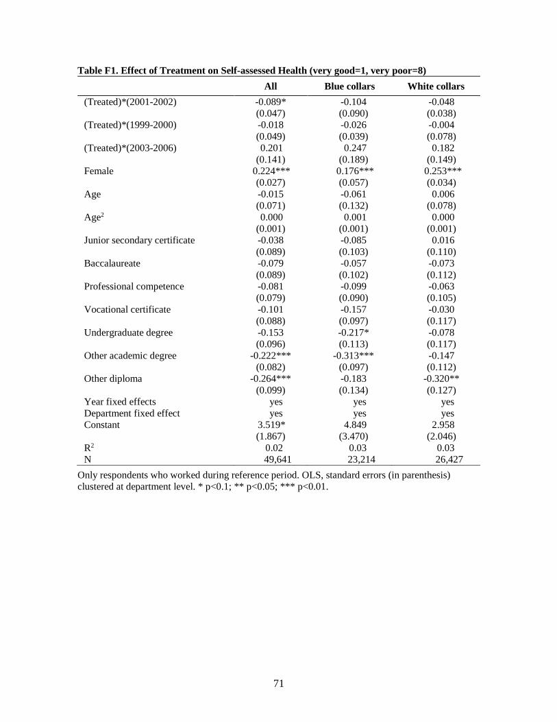
71
Table F1. Effect of Treatment on Self-assessed Health (very good=1, very poor=8) All Blue collars White collars (Treated)*(2001-2002) -0.089* -0.104 -0.048 (0.047) (0.090) (0.038) (Treated)*(1999-2000) -0.018 -0.026 -0.004 (0.049) (0.039) (0.078) (Treated)*(2003-2006) 0.201 0.247 0.182 (0.141) (0.189) (0.149) Female 0.224*** 0.176*** 0.253*** (0.027) (0.057) (0.034) Age -0.015 -0.061 0.006 (0.071) (0.132) (0.078) Age2 0.000 0.001 0.000 (0.001) (0.001) (0.001) Junior secondary certificate -0.038 -0.085 0.016 (0.089) (0.103) (0.110) Baccalaureate -0.079 -0.057 -0.073 (0.089) (0.102) (0.112) Professional competence -0.081 -0.099 -0.063 (0.079) (0.090) (0.105) Vocational certificate -0.101 -0.157 -0.030 (0.088) (0.097) (0.117) Undergraduate degree -0.153 -0.217* -0.078 (0.096) (0.113) (0.117) Other academic degree -0.222*** -0.313*** -0.147 (0.082) (0.097) (0.112) Other diploma -0.264*** -0.183 -0.320** (0.099) (0.134) (0.127) Year fixed effects yes yes yes Department fixed effect yes yes yes Constant 3.519* 4.849 2.958 (1.867) (3.470) (2.046) R2 0.02 0.03 0.03 N 49,641 23,214 26,427
Only respondents who worked during reference period. OLS, standard errors (in parenthesis) clustered at department level. * p<0.1; ** p<0.05; *** p<0.01.

72
Table F2. Effect of Treatment on Self-assessed Health (good=1, suboptimum=0) All Blue collars White collars (Treated)*(2001-2002) 0.014 0.027 -0.009 (0.015) (0.017) (0.012) (Treated)*(1999-2000) 0.014 0.009 0.021 (0.021) (0.014) (0.032) (Treated)*(after 2002) -0.026 -0.058 -0.006 (0.050) (0.058) (0.067) Female -0.050*** -0.044*** -0.055*** (0.008) (0.017) (0.009) Age -0.004 -0.009 -0.002 (0.017) (0.036) (0.019) Age2 0.000 0.000 -0.000 (0.000) (0.000) (0.000) Junior secondary certificate 0.036* 0.039** 0.029 (0.020) (0.019) (0.029) Baccalaureate 0.040** 0.032 0.041 (0.019) (0.020) (0.027) Professional competence 0.036** 0.037** 0.034 (0.017) (0.018) (0.027) Vocational certificate 0.044** 0.053*** 0.031 (0.018) (0.019) (0.028) Undergraduate degree 0.046** 0.062*** 0.028 (0.019) (0.019) (0.028) Other academic degree 0.060*** 0.067*** 0.050* (0.017) (0.019) (0.028) Other diploma 0.062*** 0.063** 0.059** (0.018) (0.026) (0.026) Year fixed effects yes yes yes Department fixed effect yes yes yes N 49,619 23,209 26,401
Only respondents who worked during reference period. Probit model (marginal effects shown), standard errors (in parenthesis) clustered at department level. * p<0.1; ** p<0.05; *** p<0.01.

73

74
Table F3. Effect of Treatment on Smoking (yes=1, no=0) All Blue collars White collars (Treated)*(2001-2002) -0.001 -0.005 -0.000 (0.015) (0.010) (0.036) (Treated)*(1999-2000) 0.032*** 0.019** 0.045** (0.007) (0.008) (0.020) (Treated)*(2003-2006) -0.041 -0.053 -0.042 (0.052) (0.043) (0.055) Female -0.029*** -0.006 -0.052*** (0.008) (0.016) (0.012) Age -0.021 0.001 -0.030 (0.023) (0.044) (0.023) Age2 0.000 -0.000 0.000 (0.000) (0.000) (0.000) Junior secondary certificate 0.045* 0.009 0.100** (0.023) (0.024) (0.044) Baccalaureate 0.025 -0.002 0.071 (0.022) (0.027) (0.046) Professional competence 0.022 -0.014 0.085* (0.019) (0.020) (0.043) Vocational certificate 0.031 -0.007 0.089* (0.022) (0.021) (0.046) Undergraduate degree 0.039 -0.006 0.098* (0.031) (0.029) (0.054) Other academic degree -0.006 -0.052*** 0.042 (0.020) (0.018) (0.042) Other diploma 0.002 -0.008 0.026 (0.028) (0.035) (0.043) Year fixed effects yes yes yes Department fixed effect yes yes yes N 48,713 22,785 25,841
Only respondents who worked during reference period. Probit model (marginal effects shown), standard errors (in parenthesis) clustered at department level. * p<0.1; ** p<0.05; *** p<0.01.
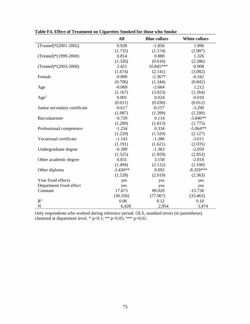
75
Table F4. Effect of Treatment on Cigarettes Smoked for those who Smoke All Blue collars White collars (Treated)*(2001-2002) 0.928 -1.856 1.996 (1.735) (1.574) (2.907) (Treated)*(1999-2000) 0.814 0.880 1.326 (1.326) (0.616) (2.286) (Treated)*(2003-2006) 2.451 10.845*** -0.908 (1.674) (2.141) (3.082) Female -0.800 -2.367* -0.342 (0.706) (1.344) (0.842) Age -0.069 -2.664 1.212 (1.167) (3.023) (1.264) Age2 0.001 0.024 -0.010 (0.011) (0.030) (0.012) Junior secondary certificate -0.617 -0.157 -3.290 (1.087) (1.399) (2.200) Baccalaureate -0.729 0.114 -3.846** (1.289) (1.813) (1.775) Professional competence -1.254 0.334 -5.064** (1.229) (1.520) (2.127) Vocational certificate -1.143 -1.386 -3.011 (1.191) (1.621) (2.035) Undergraduate degree -0.399 -1.363 -2.059 (1.525) (1.859) (2.853) Other academic degree 0.831 3.158 -2.818 (1.494) (2.132) (2.100) Other diploma -3.430** 0.092 -8.359*** (1.528) (2.019) (2.363) Year fixed effects yes yes yes Department fixed effect yes yes yes Constant 17.673 89.020 -15.736 (30.356) (77.067) (33.463) R2 0.06 0.12 0.10 N 6,428 2,954 3,474
Only respondents who worked during reference period. OLS, standard errors (in parenthesis) clustered at department level. * p<0.1; ** p<0.05; *** p<0.01.