DIION PAPER ERIE - docs.iza.org

DISCUSSION PAPER SERIES

IZA DP No. 11157

Xavier RamosDirk Van de Gaer

Is Inequality of Opportunity Robust to the Measurement Approach?

NOVEMBER 2017

Any opinions expressed in this paper are those of the author(s) and not those of IZA. Research published in this series may include views on policy, but IZA takes no institutional policy positions. The IZA research network is committed to the IZA Guiding Principles of Research Integrity.The IZA Institute of Labor Economics is an independent economic research institute that conducts research in labor economics and offers evidence-based policy advice on labor market issues. Supported by the Deutsche Post Foundation, IZA runs the world’s largest network of economists, whose research aims to provide answers to the global labor market challenges of our time. Our key objective is to build bridges between academic research, policymakers and society.IZA Discussion Papers often represent preliminary work and are circulated to encourage discussion. Citation of such a paper should account for its provisional character. A revised version may be available directly from the author.

Schaumburg-Lippe-Straße 5–953113 Bonn, Germany

Phone: +49-228-3894-0Email: [email protected] www.iza.org

IZA – Institute of Labor Economics

DISCUSSION PAPER SERIES

IZA DP No. 11157

Is Inequality of Opportunity Robust to the Measurement Approach?

NOVEMBER 2017

Xavier RamosUniversitat Autònoma de Barcelona, IZA and EQUALITAS

Dirk Van de GaerGhent University and CORE, Université Catholique de Louvain

ABSTRACT

IZA DP No. 11157 NOVEMBER 2017

Is Inequality of Opportunity Robust to the Measurement Approach?*

Recent literature has suggested many ways of measuring equality of opportunity. We

analyze in a systematic manner the various approaches put forth in the literature to show

whether and to what extent different choices matter empirically. We use EU-SILC data for

most European countries for 2005 and 2011. The choice between ex-ante and ex-post

approaches is crucial and has a substantial influence on inequality of opportunity country

orderings. Growth regressions also illustrate the relevance of conceptual choices. We only

find significant negative effects for some direct parametric ex-ante measures.

JEL Classification: D3, D63

Keywords: equality of opportunity, measurement, ex-ante, ex-post, direct approach, indirect approach, responsibility, effort, income, EU-SILC

Corresponding author:Xavier RamosUniversitat Autònoma de BarcelonaDepart Econ AplicadaCampus UABBellaterra 08193Spain

E-mail: [email protected]

* We are very grateful for comments from participants at the Seventh ECINEQ2017 Meeting in New York City. Both

authors acknowledge financial support of project ECO2016-76506-C4-4-R (Ministerio de Ciencia y Tecnología) and

Xavier Ramos acknowledges financial support of project 2014SGR-1279 (Direcció General de Recerca).

1 Introduction

Responsibility-sensitive egalitarianism shifts the focus from outcomes to their determi-

nants, when assessing economic inequalities, and advocates offsetting the effect of circum-

stances, for which individuals are not deemed responsible, while respecting the effects of

effort. Since the first contributions by Dworkin (1981), Arneson (1989), and Cohen (1990),

the economics literature, following seminar contributions by (Roemer, 1993, 1998), Fleur-

baey (1995) and Bossert (1995), has laid out the basic principles that ought to guide

measurement. In a recent paper (Ramos and Van de gaer, 2016), we bring together the

theoretical and the empirical literature and draw attention to the conceptual differences

of the empirical measures. This paper takes those lessons as starting point with the in-

tention to investigate whether those important conceptual differences have any bearing in

ordering distributions when taken to the data, and bring about systematic differences in

orderings. To this end, we estimate a wide range of inequality of opportunity measures to

the same set of data, the European Union - Statistics on Income and Living Conditions

(EU-SILC), an empirical exercise which has not been done so far.

Conceptually, the most frequently used measures of inequality of opportunity can be

classified on the basis of three criteria. The first criterion, distinguishes between ex-ante

and ex-post measures. Ex-ante measures compute the inequality in the values of indi-

viduals’ opportunity sets while ex-post measures compute the inequality in the incomes

of those that have the same efforts. Initially, the theoretical literature treated ex-ante

and ex-post approaches approaches as being very similar (Roemer, 2002, Roemer et al.,

2003). Recent theoretical contributions stress they are different and often conflict (Ooghe

et al., 2007, Roemer, 2012 and Fleurbaey and Peragine, 2013). Most of the empirical

litterature continues to treat them as interchangeable, by motivating their concern with

inequality of opportunity from ex-post intuitions and using ex-ante measures of inequality

of opportunity. We find that the distiction between ex-ante versus ex-post matters a lot

for country orderings. The second criterion, due to Pistolesi (2009), distinguishes between

direct and indirect measures. Direct measures calculate the inequality in a counterfac-

tual income distribution where all income inequalities are exclusively due to individuals’

circumstances. Indirect measures calculate the difference between the inequality in the

actual income distribution and the inequality in a counterfactual income distribution in

which there is no inequality of opportunity. Our results suggest that the distinction be-

tween direct and indirect measures is of secondary importance: conditional on the ex-ante

or ex-post apporoach, direct measures are quite different from indirect measures. The

third criterion focuses on whether a parametric or non-parametric methodology is used

to construct the counterfactual. This choice is relevant when the often-used parsimonious

linear specification does not yield a reasonable fit, and it is thus data-dependent.

In the next Section we provide a more detailed description of these criteria, present

and formally define the most frequently used measures of inequality of opportunity and

classify them. Section 3 describes the EU-SILC data and the circumstances and effort

2

variables used in the empirical analysis, while Section 4 reports our main results. We

first examine the incidence of choices on country orderings, and then show estimates from

growth regressions to illustrate further their empirical relevance. The concluding section

wraps up.

2 Measurement Approaches

As responsibility-sensitive egalitarianism distinguishes between efforts and circumstances,

the empirical model assumes that for each individual k in the population N = {1, · · · , n},his income, yk, depends on his circumstances, given by a dC-dimensional vector aCk , his

efforts, given by a dR-dimensional vector aRk , and a random term ek, such that

yk = g(aCk , a

Rk , ek

)where g : Rd

C × RdR × R→ R++.

1

Following Roemer (1993) (Peragine, 2004) a type (tranche) is a set of people having the

same circumstances (efforts). Measures of inequality of opportuity can be classified on the

basis of three criteria: whether they take an ex-ante or ex-post perspective, whether they

are direct or indirect measures of inequality of opportunity, and whether the counterfactual

distribution used in the measure is constructed using a parametric or non-parametric

method.

A first distinction is between ex-ante and ex-post approaches. The ex-ante approach

measures the inequality between individuals’ opportunity sets, and assumes that these

opportunity sets are determined by individuals’ circumstances. It attaches the same value

to the opportunity set of those that belong to the same type, and measures the inequality in

the values of individuals’ opportunity sets. The ex-post approach measures the inequality

in the incomes of individuals that have the same effort. All inequalities between such

individuals must be due to their circumstances, and is, for that reason a measure of

inequality of opportunity.2

A second distinction is between direct and indirect measures. Direct measures of

inequality of opportunity compute the inequality in a n-dimensional counterfactual income

distribution yc in which all inequalities due to differences in effort have been eliminated

such that only the inequality that is due to differences in circumstances is left:

I (yc) , (1)

where I : Rn++ → R is a measure of inequality. Indirect measures of inequality of opportu-

nity compare the inequality in the actual distribution of income, I (y), to the inequality in

1We discussed the consequences of unobserved random variation in Ramos and Van de gaer (2016), andabstract from that complication here.

2In parametric ex-post approaches the random term is put equal to zero in the construction of thecounterfactual, such that variation in the counterfactual is due to differences in efforts. In non-parametricapproaches random terms are not taken into account, but the averaging procedures make them disappear,at least asymptotically.

3

a counterfactual income distribution where there is no inequality of opportunity I(yE0).

This results in the measure

ΘI

(y, yEO

)= I (y)− I

(yEO

), (2)

where ΘI

(y, yEO

): Rn++×Rn++ → R. Based on a decomposition argument, the idea behind

the appraoch is that the difference beween the inequality in the actual distribution and

the inequality in the counterfactual income distribution without inequality of opportunity

gives the inequality that is due to inequality of opportunity.

A third distinction is based on the method used to construct the counterfactual. This

method can be parametric or non-parametric. The parametric approach imposes a func-

tional form to estimate individuals’ incomes as a function of efforts or circumstances,

resulting in specifications with 3 possible domains:

g(aCk , a

Rk , ek

)where g : Rd

C × RdR × R→ R++,

gC(aCk , ek

)where gC : Rd

C × R→ R++,

gR(aRk , ek

)where gR : Rd

R × R→ R++.

These equations can be used to estimate yk by setting ek equal to zero. Non-parametric

procedures typically do not impose a functional form and rely on averaging procedures.

Table 1 uses the three distinctions to classify the standard measures used in the liter-

ature.

Table 1: Measures of inequality of opportunity

Non-parametric Parametric

(a) Direct I (yc)

Ex-ante yc1k = 1|Nk.|

∑i∈Nk.

yi yc3k = gC(aCk , 0

)yc2k = 2

|Nk.||Nk.+1|∑

i∈Nk.iyi

Ex-post yc4k = ykµ(y)

yEO1k

yc5k(aR)

= g(aCk , a

R, 0)

(b) Indirect ΘI

(y, yEO

)= I (y)− I

(yEO

)Ex-ante yEO4

k = ykµ(y)yc1k

Ex-post yEO1k = 1

|N.k|∑

i∈N.kyi yEO3

k = gR(aRk , 0

)yEO2k = 2

|N.k||N.k+1|∑

i∈N.kiyi yEO5

k

(aC)

= g(aC , aRk , 0

)Notes: Nk. =

{i ∈ N | aCi = aCk

}, yi is the i−th largest level of income in

the set Nk., aR is a reference value for the vector of responsibility variables,

N.k ={i ∈ N | aRi = aRk

}, yi is the i−th largest level of income in the set

N.k, aC is a reference value for the vector of circumstance variables, µ (y) ismean income of vector y.

Consider the direct measures first. Three ways to measure the value of an individ-

ual’s opportunity set are proposed. Counterfactual yc1, proposed by Van de gaer (1993),

measures the value of an individual’s opportunity set by the average income of his type;

4

yc2, proposed by Lefranc et al. (2008) measures it by the normalized surface under the

generalised Lorenz curve of his type; yc3, proposed by Ferreira and Gignoux (2011) takes

the parametric estimate of his income, given his circumstances. The counterfactual for

ex-post measure yc4, proposed by Checchi and Peragine (2010), scales everybody’s income

up or down by the ratio of the average income in the population and the average income

of his tranche. That way, the inequalities between those that belong to the same tranche

are preserved, while the differences in average incomes of different tranches are eliminated.

Finally, yc5, proposed by Pistolesi (2009), relies on the choice of aR, a reference value for

the vector of responsibility characteristics and takes the parametric estimate of his income,

given his circumstances and efforts equal to the reference values.

The counterfactuals used in the indirect approach are obtained by switching the role of

circumstance and effort variables of the direct approach. This dual relationship is reflected

in the number used to label the counterfactuals: for all i = 1, · · · , 5, yEOi is the dual

counterfactual of yci. Checchi and Peragine (2010) proposed counterfactual yEO1, which

assigns to every individual the average income of his tranche; yEO2 assigns the value of the

normalized surface under the generalised Lorenz curve of the income distribution of his

tranche; yEO3 the parametric estimate of his income, given his efforts; yEO5 the parametric

estimate of his income, given his efforts and circumstances equal to the reference values. In

all these counterfactuals, those with the same efforts have the same income, such that the

corresponding indirect measure becomes a measure of the income inequality that is due to

their different circumstance; they are ex-post measures of inequality of opportunity. The

only ex-ante measure is yEO4, proposed by Checchi and Peragine (2010), where incomes

are scaled up or down by the ratio of the average income in the population and the value of

the opportunity set measured by yc1k , such that in this counterfactual, the average income

of every type equals average income in the population and everyone’s opportunity set has

the same value. In the sequel IX denotes the inequality measure based on counterfactual

yX with X ∈ {c1, . . . , c5, EO1, . . . , EO5}.

3 Data

We draw on data from the European Union - Statistics on Income and Living Conditions

(EU-SILC), which collects comparable information on socio-economic and demographic

characteristics of individuals across European countries. In particular we use the 2005

and 2011 waves, which collected information on family background and circumstances

when the respondent was young in separate questionnaire modules. EU-SILC data have

been commonly used to study equality of opportunity across European countries, see inter

alia Marrero and Rodrıguez (2012) and Checchi et al. (2016).

The EU-SILC provides data for a large number of countries, which allows us to compare

country orderings by inequality of opportunity when different measures are used. The main

limitation of EU-SILC is the reduced sample sizes for some countries, which obliges us to

work with a reduced number of circumstances and efforts.

5

As in previous studies, e.g. Marrero and Rodrıguez (2012), we select individuals aged

25 to 59 to avoid the noise associated to the school-job transition for the younger popula-

tion and to retirement decisions for the older individuals.

Our outcome of interest is disposable equivalent income.3 To check the reliability of our

income variable, we compare our income inequality estimates with other estimates coming

from different sources, such as the OECD, and obtain correlation coefficients above 0.9,

indicating that our estimates are in line with those from the OECD.

Working with a limited amount of circumstances and effort variables, and thus types

and tranches, results in partitions that are too coarse and that end up driving the estimates

of the various direct and indirect measures. Because of this, we use a set of 5 circumstance

and 4 effort variables, which translate into 48 types and 24 tranches, thus achieving finer

partitions than the majority of recent empirical studies on equality of opportunity. Our

circumstances include parental education and occupation, gender, birthplace, and whether

the respondent lived with both parents when young, while the set of efforts includes own

educational attainment, own occupation, work status, and marital status. All variables

have two categories, except the two occupation variables, which have 3 categories each.

Description and summary statistics of circumstance and effort variables can be found in

Appendix Tables 10 to 13.

The circumstance variable “whether both parents were present at home when respon-

dent was young” has not been used before, and thus deserve some justification. Growing

up in non-intact families is found to condition several later-life outcomes, and earnings

during adulthood is one of them (Mohanty and Ullah, 2012).

Own education has been previously used as effort variable (e.g. Almas et al., 2011),

but we believe deserves some discussion. Undoubtedly own effort affects educational at-

tainment (De Fraja et al., 2010), which in turn determines wages and thus incomes. What

may be a bit more controversial is the choice of own education as an effort variable, as

some may argue that children cannot be deemed responsible for their own effort before

the age of consent, and such effort levels are also determining later educational attainment

after the age of consent. As discussed above, however, since there are only few variables

in the EU-SILC that can be used as effort variables and most of them provide only very

small cell sizes, we decided to use own educational attainment as an effort variable.

The other variables included in the set of circumstances or effort are not new and

rather uncontroversial, and do not deserve further discussion.4

3Disposal equivalent individual income is computed by deflating disposal equivalent household income(variable HY020, including the sum for all household members of gross personal income components plusgross income components at household level, minus taxes paid), with the modified OECD equivalent scale,(variable HX050, which assigns a weight of 1 to the first adult, of 0.5 to remaining adults of the family,and of 0.3 to children younger than 14).

4See Table 25.8 in Ferreira and Peragine (2016) for a list of circumstance variables used in eight papersthat cover 41 countries. Roemer and Trannoy (2015) discuss important issues in the use of effort variablesoften included in empirical analyses.

6

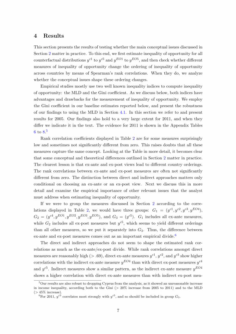
4 Results

This section presents the results of testing whether the main conceptual issues discussed in

Section 2 matter in practice. To this end, we first estimate inequality of opportunity for all

counterfactual distributions yc1 to yc5 and yEO1 to yEO5, and then check whether different

measures of inequality of opportunity change the ordering of inequality of opportunity

across countries by means of Spearman’s rank correlations. When they do, we analyze

whether the conceptual issues shape these ordering changes.

Empirical studies mostly use two well known inequality indices to compute inequality

of opportunity: the MLD and the Gini coefficient. As we discuss below, both indices have

advantages and drawbacks for the measurement of inequality of opportunity. We employ

the Gini coefficient in our baseline estimates reported below, and present the robustness

of our findings to using the MLD in Section 4.1. In this section we refer to and present

results for 2005. Our findings also hold to a very large extent for 2011, and when they

differ we indicate it in the text. The evidence for 2011 is shown in the Appendix Tables

6 to 8.5

Rank correlation coefficients displayed in Table 2 are for some measures surprisingly

low and sometimes not significantly different from zero. This raises doubts that all these

measures capture the same concept. Looking at the Table in more detail, it becomes clear

that some conceptual and theoretical differences outlined in Section 2 matter in practice.

The clearest lesson is that ex-ante and ex-post views lead to different country orderings.

The rank correlations between ex-ante and ex-post measures are often not significantly

different from zero. The distinction between direct and indirect approaches matters only

conditional on choosing an ex-ante or an ex-post view. Next we discuss this in more

detail and examine the empirical importance of other relevant issues that the analyst

must address when estimating inequality of opportunity.

If we were to group the measures discussed in Section 2 according to the corre-

lations displayed in Table 2, we would have three groups: G1 = (yc1, yc2, yc3, yEO4),

G2 = (yc4, yEO1, yEO2, yEO3, yEO5), and G3 = (yc5). G1 includes all ex-ante measures,

while G2 includes all ex-post measures but yc5, which seems to yield different orderings

than all other measures, so we put it separately into G3. Thus, the difference between

ex-ante and ex-post measures comes out as an important empirical divide.6

The direct and indirect approaches do not seem to shape the estimated rank cor-

relations as much as the ex-ante/ex-post divide. While rank correlations amongst direct

measures are reasonably high (> .69), direct ex-ante measures yc1, yc2, and yc3 show higher

correlations with the indirect ex-ante measure yEO4 than with direct ex-post measures yc4

and yc5. Indirect measures show a similar pattern, as the indirect ex-ante measure yEO4

shows a higher correlation with direct ex-ante measures than with indirect ex-post mea-

5Our results are also robust to dropping Cyprus from the analysis, as it showed an unreasonable increasein income inequality, according both to the Gini (> 20% increase from 2005 to 2011) and to the MLD(> 45% increase).

6For 2011, yc3 correlates most strongly with yc5, and so should be included in group G3.

7

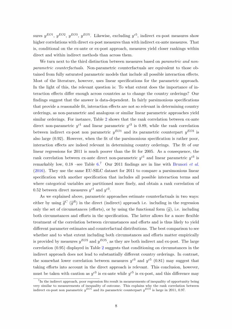
sures yEO1, yEO2, yEO3, yEO5. Likewise, excluding yc5, indirect ex-post measures show

higher correlations with direct ex-post measures than with indirect ex-ante measures. That

is, conditional on the ex-ante or ex-post approach, measures yield closer rankings within

direct and within indirect methods than across them.

We turn next to the third distinction between measures based on parametric and non-

parametric counterfactuals. Non-parametric counterfactuals are equivalent to those ob-

tained from fully saturated parametric models that include all possible interaction effects.

Most of the literature, however, uses linear specifications for the parametric approach.

In the light of this, the relevant question is: To what extent does the importance of in-

teraction effects differ enough across countries as to change the country orderings? Our

findings suggest that the answer is data-dependent. In fairly parsimonious specifications

that provide a reasonable fit, interaction effects are not so relevant in determining country

orderings, as non-parametric and analogous or similar linear parametric approaches yield

similar orderings. For instance, Table 2 shows that the rank correlation between ex-ante

direct non-parametric yc1 and linear parametric yc3 is 0.89, while the rank correlation

between indirect ex-post non parametric yEO1 and its parametric counterpart yEO3 is

also large (0.92). However, when the fit of the parsimonious specification is rather poor,

interaction effects are indeed relevant in determining country orderings. The fit of our

linear regressions for 2011 is much poorer than the fit for 2005. As a consequence, the

rank correlation between ex-ante direct non-parametric yc1 and linear parametric yc3 is

remarkably low, 0.18 –see Table 6.7 Our 2011 findings are in line with Brunori et al.

(2016). They use the same EU-SILC dataset for 2011 to compare a parsimonious linear

specification with another specification that includes all possible interaction terms and

where categorical variables are partitioned more finely, and obtain a rank correlation of

0.52 between direct measures yc1 and yc3.

As we explained above, parametric approaches estimate counterfactuals in two ways:

either by using gC (gR) in the direct (indirect) approach i.e. including in the regression

only the set of circumstances (efforts), or by using the functional form (g), i.e. including

both circumstances and efforts in the specification. The latter allows for a more flexible

treatment of the correlation between circumstances and efforts and is thus likely to yield

different parameter estimates and counterfactual distributions. The best comparison to see

whether and to what extent including both circumstances and efforts matter empirically

is provided by measures yEO3 and yEO5, as they are both indirect and ex-post. The large

correlation (0.95) displayed in Table 2 suggests that conditioning on circumstances in the

indirect approach does not lead to substantially different country orderings. In contrast,

the somewhat lower correlation between measures yc3 and yc5 (0.81) may suggest that

taking efforts into account in the direct approach is relevant. This conclusion, however,

must be taken with caution as yc3 is ex-ante while yc5 is ex-post, and this difference may

7In the indirect approach, poor regression fits result in measurements of inequality of opportunity beingvery similar to measurements of inequality of outcome. This explains why the rank correlation betweenindirect ex-post non parametric yEO1 and its parametric counterpart yEO3 is large in 2011, 0.97.

8

also be behind the lower correlation.

Dual counterfactuals provide a somewhat natural way of making conceptual analogies

between views and approaches. The data reveal that they lead to country orderings that

are quite different –rank correlation coefficients amongst dual counterfactuals range from

0.11 to 0.41. Moreover, in our grouping of measures on the basis of their correlation, it

never happens that dual counterfactuals belong to the same group.

Finally we examine whether it matters allowing for inequality aversion with respect to

income differences due to differences in effort. We compare the non-parametric measures,

yc1 and yc2 for the direct approach, and yEO1 and yEO2 for the indirect approach. The

results in Table 2 show that allowing for inequality aversion does not matter neither for

the direct nor for the indirect measures, as rank correlations are larger than 0.93.

Table 2: Rank correlations between inequality of opportunity measures. Ginicoefficient, 2005.

Direct measures Indirect MeasuresEA EP EA

yc1 yc2 yc3 yc4 yc5 yEO1 yEO2 yEO3 yEO4

yc2 0.9680.000

yc3 0.894 0.9160.000 0.000

yc4 0.729 0.740 0.7020.000 0.000 0.000

yc5 0.759 0.829 0.814 0.6850.000 0.000 0.000 0.000

yEO1 0.412 0.389 0.279 0.794 0.4140.037 0.050 0.168 0.000 0.036

yEO2 0.232 0.225 0.159 0.733 0.299 0.9280.256 0.257 0.438 0.000 0.138 0.000

yEO3 0.221 0.186 0.110 0.647 0.196 0.915 0.9320.278 0.364 0.594 0.000 0.338 0.000 0.000

yEO4 0.964 0.931 0.841 0.639 0.695 0.321 0.174 0.1670.000 0.000 0.000 0.000 0.000 0.110 0.395 0.416

yEO5 0.394 0.368 0.287 0.740 0.346 0.917 0.901 0.952 0.3470.046 0.065 0.155 0.000 0.083 0.000 0.000 0.000 0.082

Notes: Rank correlations are shown in the upper row, while p-values are shown inthe lower row. EA means Ex-ante, EP means Ex-post.

9

4.1 Robustness to using the MLD instead of the Gini

The high cross index correlations of Table 5 show that using the Gini coefficient or the MLD

does not matter much for our country orderings. Table 4 shows that our findings about the

correlations between the different measures also hold for the MLD index. It is striking,

however, that the correlations between ex-ante and ex-post measures are substantially

higher for the MLD than for the Gini.8 Due to its path independence property (Foster

and Sneyerov, 2000), yc1 and yEO4, as well as yEO1 and yc4 yield exactly the same ordering

when using the MLD. The other indirect counterfactuals give a distribution in which all

inequality is due to differences in efforts, and, a decomposition argument can be used to

say that the difference in inequality in the actual distribution and the inequality that is due

to efforts equals the inequality that is due to circumstances, which is what direct measures

capture. Our finding that the rank correlations between ex-ante and ex-post measures are

larger for the MLD than for the Gini confirms that the decomposition argument makes

more sense for the MLD than for the Gini coefficient.

4.2 Inequality of Opportunity and Economic Growth

To illustrate further the empirical relevance of the different conceptual choices, this sec-

tion explores the relationship between inequality of opportunity and economic growth,

which has captured the attention of the recent literature. It is important to note that

given the many limitations that the EU-SILC imposes, this empirical exercise is solely

illustrative. As outlined in Section 3, the EU-SILC collects data on family background

and circumstances when the respondent was young at two points in time, 2005 and 2011.

This means that we can only estimate inequality of opportunity for these two years. This

data structure imposes two major limitations on our empirical exercise: First, our time

series is very short, as we can only exploit variability at two points in time, and second,

we can only study growth over a time period which is much shorter than the 5 or 10 year

period, which is customary.

Recent literature has explored the idea that inequality due to efforts and inequality

due to circumstances (inequality of opportunity) have opposite effects on economic growth,

which in turn may help explain the inconclusive evidence of the effects of overall inequality

on economic growth (see among others Marrero and Rodrıguez, 2013 and Ferreira et al.,

2014). While inequality of opportunity is argued to have a deleterious impact on economic

growth, effort inequality is deemed to have an enhancing impact on growth. The empirical

papers that test this hypothesis usually use only one of the many options outlined in

Section 2 to estimate inequality of opportunity. However, as we have reported above,

different opportunity inequality measures give rise to different country orderings. Do the

findings reported in the literature crucially hinge on the specific inequality of opportunity

measure used? To answer this question, this section runs growth regressions and checks

8The same is true for the correlation between yEO4 and the other indirect measures, but remember thatthe former produces rankings that are more similar to the ones produced by ex-ante measures.

10

whether results are robust to the way inequality of opportunity and inequality of effort

are measured.

Following Forbes (2000), we estimate the following panel regression

gc,(t,t−s) = β1IOc,t−s + β2IEc,t−s + β3GDPc,t−s + β4Edc,t−s + β5Invc,t−s + αc + τt + εct

where gct is the average annual growth rate of per capita GDP between t and t − s,IOc,t−s is one of the inequality of opportunity measures outlined in Section 2, IEc,t−s is

residual inequality, often assumed to be inequality of effort, and computed as the difference

between outcome and opportunity inequality, GDPc,t−s is the Gross Domestic Product,

Edc,t−s is the population share with upper secondary education or above, Invc,t−s is the

business investment to GDP ratio, and αc and τt capture country and time specific fixed

effects. Control variables, namely GDP, education shares, and investment, come from

Euorstat, and all regressors refer to the initial period over which growth is estimated to

avoid simultaneity issues.

We estimate the model by fixed effects, which control for time-invariant omitted vari-

ables. It is a demanding estimation strategy, as we are identifying effects using within-

country variation with only two time points, but nonetheless still suffers from endogeneity

problems (Bond, 2002). Given the difficulty to find external instruments, system-GMM

methods are usually employed to address such endogeneity issues (Bond et al., 2001).

These models, however, require three time points, while we only have two, which precludes

us from taking due account of the possible endogeneity bias. If we however assume that

the possible bias does not change across different measures of inequality of opportunity,

it should not invalidate our comparative results, which is what we are mainly concerned

with in this empirical exercise.

Table 3 reports the fixed effects estimates of outcome inequality and of the two variables

of interest, IOc,t−s and IEc,t−s for one to three year average annual growth rates and the

ten measures of inequality of opportunity, measured with the Gini coefficient. Outcome

inequality regressions simply replace the two inequality of opportunity and effort measures

in the specification above with a measure of outcome inequality. We find non-significant

effects of outcome inequality on growth, regardless of whether the latter is measured over

one, two or three years.

Inequality of Opportunity is only significant at the standard 5% level with the expected

negative sign when the measure yc5 is used for one- and two-year growth rates. The

measure yc3 is also negative and significant at 10% but only for three-year growth rates,

while inequality of effort is systematically not significant. Appendix Table 9 shows that

when the MLD is used to measure inequality in the counterfactual distributions inequality

of opportunity shows no significant effect on growth.9

Given the difficulty of identifying precise effects using within-country variation with

9As it happens with the correlation between different measures, our growth results are also robust todropping Cyprus from the analysis, as it showed an unreasonable increase in income inequality, accordingboth to the Gini (> 20% increase from 2005 to 2011) and to the MLD (> 45% increase).

11

only two time points, we next abstract from the precision of the point estimates, and

examine how the conceptual divides relate to the following two hypotheses about the

effects of opportunity and effort inequality.

Strong hypothesis (SH): The effect of inequality of opportunity is negative while the effect

of effort inequality is positive (i.e. β1 < 0 and β2 > 0).

Weak hypothesis (WH): The effect of inequality of opportunity is more negative than the

effect of effort inequality (i.e. 0 > β1 < β2).

The estimates reported in Table 3 show that, ignoring issues of statistical significance,

SH occurs only twice (for one-year growth), each time for ex ante measures. For indirect

measures it never happens that the two effects have opposite signs. Direct measures

are always in line with WH, except for yc4 with 3-period growth. However, for indirect

measures, this is the case in only 5 instances out of 15.10 All and all, this evidence may

be seen as a (admittedly) weak argument in support of the direct approach.

In sum, this empirical exercise illustrates that the effect of inequality of opportunity

(and effort) on growth is not robust to the measure of inequality of opportunity employed.

These findings cast doubt on existing evidence, which is exclusively based on the ex-ante

parametric measure yc3, and highlights the importance of different measurement choices.

We hope we provide grounds for the still incipient empirical literature that explores the

effects of equality of opportunity on growth to check the sensibility of its findings to

different choices.

10When we use the MLD as inequality index, our findings are also consistent with SH for ex ante (direct)measures. However, both direct and indirect measures are consistent with WH in about two thirds of thecases –Table 9 in the Appendix shows the coefficient estimates.

12

Table 3: Growth regressions. Fixed effect estimates of Outcome, Opportunity and Effort Inequality. Inequality measured with the Ginicoefficient.

Period Inequality Direct Approachy yc1 yc2 yc3 yc4 yc5

β p-value β p-value β p-value β p-value β p-value β p-value(t, t-1) Outcome -0.240 0.353

Opportunity -0.354 0.289 -0.335 0.340 -0.591 0.128 -0.280 0.332 -1.494** 0.016Effort -0.152 0.289 -0.190 0.514 0.001 0.998 -0.115 0.789 0.082 0.752

(t, t-2) Outcome -0.275 0.250Opportunity -0.440 0.151 -0.397 0.220 -0.584 0.104 -0.305 0.253 -1.248** 0.033Effort -0.147 0.595 -0.210 0.430 -0.063 0.829 -0.181 0.650 -0.025 0.921

(t, t-3) Outcome -0.340 0.157Opportunity -0.462 0.134 -0.406 0.210 -0.639* 0.076 -0.332 0.212 -1.098* 0.065Effort -0.244 0.382 -0.304 0.259 -0.134 0.645 -0.362 0.365 -0.144 0.583

Indirect ApproachyEO1 yEO2 yEO3 yEO4 yEO5

β p-value β p-value β p-value β p-value β p-value(t, t-1) Opportunity -0.219 0.482 -0.210 0.495 -0.219 0.476 -0.175 0.888 -0.178 0.576

Effort -0.242 0.365 -0.245 0.360 -0.243 0.364 -0.247 0.402 -0.246 0.357(t, t-2) Opportunity -0.271 0.347 -0.269 0.334 -0.270 0.344 -0.628 0.583 -0.234 0.426

Effort -0.276 0.265 -0.276 0.266 -0.276 0.265 -0.239 0.376 -0.279 0.259(t, t-3) Opportunity -0.303 0.290 -0.318 0.263 -0.314 0.268 -0.634 0.577 -0.282 0.335

Effort -0.342 0.167 -0.343 0.168 -0.343 0.167 -0.309 0.253 -0.344 0.164

N 49 49 49 49 49 49

Notes: All regressions include GDP, population share with upper-secondary school or above, and ratio of business investment to GDP, all measuredat the beginning of the period, plus a time dummy. * p-value<0.1, ** p-value<0.05.

13

5 Conclusion

Several choices guide the measurement of equality of opportunity. We use EU-SILC data

for many European countries to examine whether those choices matter empirically. To

this end, we perform two empirical exercises: First we check whether measures that share

the same conceptual choices yield similar inequality of opportunity country orderings, and

then we analyse whether they yield similar estimates in growth regressions.

Our findings on country orderings identify one crucially important divide, between

ex-ante and ex-post views, as it leads to different country orderings. The distinction

between direct and indirect approaches matters only conditional on choosing an ex-ante

or an ex-post view. Recent theoretical contributions have shown that ex-ante and ex-

post approaches to inequality of opportunity are incompatible. Our paper shows that the

distinction also matters empirically. As the evaluation of inequality of opportunity is in

essence a normative exercise, our results show that researchers should be explicit about the

normative choice made between an ex-ante or ex-post criterion. From growth regressions

we conclude that the particular measure of inequality of opportunity employed conditions

the effect that inequality of opportunity (and inequality due to effort) has on growth. We

find that the direct parametric ex-ante measures correlate more in the expected way with

economic growth than the others. As the question whether inequality of opportunity has

an effect on economic growth is a positive exercise, our results could suggest that it is

ex-ante inequality of opportunity (i.e. inequality between opportunity sets) rather than

ex-post inequality of opportunity that is detrimental for growth.

Hence we have to recognize that inequality of opportunity is a multifaced concept.

Consequently, scholars should provide arguments to support the conceptual choices em-

bedded in the measures they use. Particular attention should be paid to taking and ex-ante

or an ex-post view.

14

References

Almas, I., Cappelen, A. W., Lind, J. T., Sørensen, E. Ø. and Tungodden, B. (2011).

Measuring unfair (in)equality. Journal of Public Economics, 95 (7), 488–499.

Arneson, R. J. (1989). Equality and equal opportunity for welfare. Philosophical studies, 56 (1),

77–93.

Bond, S. (2002). Dynamic panel data models: A guide to micro data methods and practice.

Portuguese Economic Journal, 1 (2), 141–162.

—, Hoeffler, A. and Temple, J. (2001). GMM estimation of empirical growth models. CEPR

Discussion Paper 3048, LSE.

Bossert, W. (1995). Redistribution mechanisms based on individual characteristics. Mathematical

Social Sciences, 1 (31), 51.

Brunori, P., Peragine, V. and serlenga, L. (2016). Upwerd and downward bias when mea-

suring inequality of Opportunity. ECINEQ Working Paper Series 406, ECINEQ.

Checchi, D. and Peragine, V. (2010). Inequality of opportunity in Italy. Journal of Economic

Inequality, pp. 429–450.

—, — and Serlenga, L. (2016). Inequality of opportunity in europe: Is there a role for institu-

tions? Research in Labour Economics, 43, 1–44.

Cohen, G. A. (1990). Equality of what? On welfare, goods and capabilities. Recherches

Economiques de Louvain/Louvain Economic Review, pp. 357–382.

De Fraja, G., Oliveira, T. and Zanchi, L. (2010). Must try harder: Evaluating the role of

effort in educational attainment. Review of Economics and Statistics, 92 (3), 577–597.

Dworkin, R. (1981). What is equality? Part 2: Equality of resources. Philosophy & Public

Affairs, pp. 283–345.

Ferreira, F. H. and Gignoux, J. (2011). The measurement of inequality of opportunity: Theory

and an application to latin america. Review of Income and Wealth, 57, 622–657.

—, Lakner, C., Lugo, M. A. and Ozler, B. (2014). Inequality of Opportunity and Economic

Growth. A Cross-Country Analysis. Policy Research Working Paper Series 6915, The World

Bank.

— and Peragine, V. (2016). Individual responsibility and equality of opportunity. In M. D. Adler

and M. Fleurbaey (eds.), Oxford Handbook of Well-Being and Public Policy, Oxford University

Press, pp. 746–784.

Fleurbaey, M. (1995). The requisites of equal opportunity. Social Choice, Welfare and Ethics,

pp. 37–53.

— and Peragine, V. (2013). Ex ante versus ex post equality of opportunity. Economica, 80,

118–130.

15

Forbes, K. (2000). A reassessment of the relationship between inequality and growth. American

Economic Review, 90 (4), 869–887.

Foster, J. and Sneyerov, A. (2000). Path independent inequality measures. Journal of Eco-

nomic Theory, 91 (2), 199–222.

Lefranc, A., Pistolesi, N. and Trannoy, A. (2008). Inequality of opportunities vs. inequality

of outcomes: Are western societies all alike? Review of Income and Wealth, 54, 513–546.

Marrero, G. and Rodrıguez, J. G. (2012). Inequality of opportunity in Europe. Review of

Income and Wealth, 58 (4), 597–621.

— and Rodrıguez, J. G. (2013). Inequality of opportunity and growth. Journal of Development

Economics, 104, 107–122.

Mohanty, M. and Ullah, A. (2012). Why does growing up in an intact family during childhood

lead to higher earnings during adulthood in the United States? American Journal of Economics

and Sociology, 71 (3), 662–695.

Ooghe, E., Schokkaert, E. and Van de gaer, D. (2007). Equality of opportunity versus

equality of opportunity sets. Social Choice and Welfare, 8, 209–230.

Peragine, V. (2004). Ranking income distributions according to equality of opportunity. Journal

of Economic Inequality, 2, 11–30.

Pistolesi, N. (2009). Inequality of opportunity in the land of opportunities, 1968-2001. Journal

of Economic Inequality, 7, 411–433.

Ramos, X. and Van de gaer, D. (2016). Empirical approaches to inequality of opportunity:

Principles, measures, and evidence. Journal of Economic Surveys, 30 (5), 855–883.

Roemer, J. (2012). On several approaches to equality of opportunity. Economics and Philosophy,

28, 165–200.

Roemer, J. E. (1993). A pragmatic theory of responsibility for the egalitarian planner. Philosophy

& Public Affairs, pp. 146–166.

— (1998). Equality of Opportunity. Harvard University Press.

— (2002). Equality of opportunity: A progress report. Social Choice and Welfare, 19, 455–471.

—, Aaberge, R., Colombino, U., Fritzell, J., Jenkins, S. P., Marx, I., Page, M., Pom-

mer, E., J., R.-C., San Segundo, M. J., Tranaes, T., Wagner, G. G. and Zubiri, I.

(2003). To what extent do fiscal regimes equalize opportunities for income acquisition among

citizens? Journal of Public Economics, 87, 539–565.

— and Trannoy, A. (2015). Equality of opportunity. In A. B. Atkinson and F. Bourguignon

(eds.), Handbook of Income Distribution, Volume 2A-2B, North Holland, pp. 217–300.

Van de gaer, D. (1993). Equality of opportunity and investment in human capital. Ph.D. thesis,

Leuven: Katholieke Universiteit Leuven.

16

A Appendix

Table 4: Rank correlations between inequality of opportunity measures. MeanLog Deviation, 2005.



yc2 0.9420.000

yc3 0.895 0.9460.000 0.000

yc4 0.730 0.722 0.7440.000 0.000 0.000

yc5 0.737 0.797 0.841 0.6210.000 0.000 0.000 0.001

yEO1 0.730 0.722 0.744 1.000 0.6210.000 0.000 0.000 0.000 0.001

yEO2 0.730 0.708 0.722 0.987 0.584 0.9870.000 0.000 0.000 0.000 0.002 0.000

yEO3 0.733 0.717 0.744 0.997 0.612 0.997 0.9860.000 0.000 0.000 0.000 0.001 0.000 0.000

yEO4 1.000 0.942 0.895 0.730 0.737 0.730 0.730 0.7330.000 0.000 0.000 0.000 0.000 0.000 0.000 0.000

yEO5 0.761 0.745 0.760 0.992 0.625 0.992 0.986 0.995 0.7610.000 0.000 0.000 0.000 0.001 0.000 0.000 0.000 0.000


17

Table 5: Rank correlations between Gini- and MLD-based inequality of oppor-tunity measures, 2005.

Direct Indirectyc1 yc2 yc3 yc4 yc5 yEO1 yEO2 yEO3 yEO4 yEO5

0.976 0.975 0.974 0.982 0.964 0.809 0.755 0.693 0.963 0.7740.000 0.000 0.000 0.000 0.000 0.000 0.000 0.000 0.000 0.000

Notes: Rank correlations are shown in the upper row, while p-values are shown in thelower row.

Table 6: Rank correlations between inequality of opportunity measures. Ginicoefficient, 2011.



yc2 0.7700.000

yc3 0.181 0.4250.348 0.022

yc4 0.225 0.345 0.2350.241 0.068 0.220

yc5 0.211 0.489 0.965 0.2530.271 0.007 0.000 0.186

yEO1 -0.018 0.138 -0.011 0.875 0.0200.925 0.476 0.954 0.000 0.917

yEO2 -0.025 0.117 0.030 0.899 0.045 0.7930.790 0.547 0.881 0.000 0.815 0.000

yEO3 0.028 0.118 0.036 0.900 0.062 0.971 0.9920.885 0.541 0.853 0.000 0.749 0.000 0.000

yEO4 0.733 0.741 0.518 0.126 0.572 -0.123 -0.123 -0.0940.000 0.000 0.004 0.515 0.001 0.525 0.526 0.627

yEO5 -0.003 0.085 -0.009 0.892 0.011 0.970 0.992 0.985 -0.1470.990 0.662 0.964 0.000 0.954 0.000 0.000 0.000 0.446

Notes: Rank correlations are shown in the upper row, while p-values are shown in thelower row. EA means Ex-ante, EP means Ex-post.

18

Table 7: Rank correlations between inequality of opportunity measures. MeanLog Deviation, 2011.



yc2 0.8500.000

yc3 0.503 0.6670.005 0.000

yc4 0.358 0.336 0.2450.057 0.075 0.201

yc5 0.549 0.713 0.965 0.2620.002 0.000 0.000 0.170

yEO1 0.358 0.336 0.245 1.000 0.2620.057 0.075 0.201 0.000 0.170

yEO2 0.344 0.322 0.234 0.999 0.251 0.9990.068 0.088 0.223 0.000 0.189 0.000

yEO3 0.344 0.322 0.234 1.000 0.251 1.000 0.9990.068 0.089 0.223 0.000 0.190 0.000 0.000

yEO4 1.000 0.849 0.503 0.358 0.549 0.358 0.343 0.3440.000 0.000 0.005 0.057 0.002 0.057 0.067 0.068

yEO5 0.358 0.336 0.245 1.000 0.262 1.000 0.995 1.000 0.3580.057 0.075 0.201 0.000 0.170 0.000 0.000 0.000 0.057


Table 8: Rank correlations between Gini- and MLD-based inequality of oppor-tunity measures, 2011.

Direct Indirectyc1 yc2 yc3 yc4 yc5 yEO1 yEO2 yEO3 yEO4 yEO5

0.781 0.817 0.981 0.980 0.982 0.873 0.887 0.886 0.928 0.8650.000 0.000 0.000 0.000 0.000 0.000 0.000 0.000 0.000 0.000

Notes: Rank correlations are shown in the upper row, while p-values are shown in thelower row.

19

Table 9: Growth regressions. Fixed effect estimates of Outcome, Opportunity and Effort Inequality. Inequality measured with theMean Log Deviation.

Period Inequality Direct Approachy yc1 yc2 yc3 yc4 yc5

β p-value β p-value β p-value β p-value β p-value β p-value(t, t-1) Outcome -0.180 0.393

Opportunity -0.351 0.739 0.372 0.764 0.358 0.788 -0.209 0.412 -5.892 0.376Effort -0.157 0.541 -0.237 0.346 -0.234 0.358 -0.117 0.744 -0.103 0.653

(t, t-2) Outcome -0.203 0.298Opportunity -0.610 0.529 0.072 0.950 0.207 0.866 -0.233 0.324 -4.376 0.478Effort -0.149 0.527 -0.231 0.320 -0.244 0.300 -0.139 0.673 -0.147 0.492

(t, t-3) Outcome -0.243 0.216Opportunity -0.552 0.569 0.178 0.876 0.202 0.869 -0.240 0.310 -1.663 0.788Effort -0.202 0.394 -0.286 0.221 -0.288 0.224 -0.250 0.452 -0.224 0.305

Indirect ApproachyEO1 yEO2 yEO3 yEO4 yEO5

(t, t-1) Opportunity -0.209 0.412 -0.204 0.431 -0.197 0.456 -0.351 0.739 -0.160 0.549Effort -0.117 0.744 -0.132 0.708 -0.148 0.679 -0.157 0.541 -0.222 0.578



N 49 49 49 49 49 49

Notes: All regressions include GDP, population share with upper-secondary school or above, and ratio of business investment to GDP, all measuredat the beginning of the period, plus a time dummy. * p-value<0.1, ** p-value<0.05.

20

Table 10: Summary Statistics of Circumstance Variables, 2005

Parental Education Parental Occupation

Country >Secondary Skilled Unskilled Male Foreign Parents at home

BE Belgium 0.19 0.41 0.21 0.49 0.08 0.890.39 0.49 0.40 0.50 0.26 0.32

DK Denmark 0.22 0.45 0.20 0.49 0.04 0.840.41 0.50 0.40 0.50 0.19 0.37

DE Germany 0.34 0.45 0.18 0.44 0.05 0.850.47 0.50 0.38 0.50 0.23 0.36

GR Greece 0.08 0.67 0.15 0.49 0.06 0.950.27 0.47 0.36 0.50 0.24 0.22

ES Spain 0.09 0.53 0.30 0.48 0.05 0.910.29 0.50 0.46 0.50 0.21 0.29

FR France 0.10 0.43 0.29 0.48 0.09 0.840.30 0.50 0.45 0.50 0.29 0.37

IE Ireland 0.13 0.27 0.29 0.47 0.03 0.920.34 0.44 0.45 0.50 0.17 0.27

IT Italy 0.03 0.49 0.28 0.49 0.04 0.920.18 0.50 0.45 0.50 0.20 0.27

LU Luxembourg 0.18 0.40 0.28 0.49 0.09 0.900.39 0.49 0.45 0.50 0.28 0.31

NL Netherlands 0.17 0.34 0.17 0.49 0.05 0.900.37 0.48 0.37 0.50 0.21 0.30

AT Austria 0.06 0.56 0.22 0.49 0.09 0.850.24 0.50 0.42 0.50 0.29 0.36

PT Portugal 0.04 0.63 0.24 0.48 0.01 0.850.19 0.48 0.43 0.50 0.11 0.36

FI Finland 0.15 0.57 0.20 0.50 0.02 0.850.36 0.50 0.40 0.50 0.12 0.35

SE Sweden 0.21 0.49 0.18 0.49 0.08 0.830.41 0.50 0.38 0.50 0.28 0.38

UK United Kingdom 0.33 0.36 0.31 0.48 0.10 0.840.47 0.48 0.46 0.50 0.31 0.37

CY Cyprus 0.07 0.57 0.31 0.47 0.09 0.910.26 0.50 0.46 0.50 0.29 0.29

CZ Czech Rep. 0.09 0.50 0.28 0.48 0.01 0.860.29 0.50 0.45 0.50 0.10 0.35

EE Estonia 0.25 0.38 0.39 0.46 0.15 0.760.43 0.49 0.49 0.50 0.36 0.43

HU Hungary 0.13 0.52 0.30 0.48 0.02 0.840.34 0.50 0.46 0.50 0.14 0.37

LV Latvia 0.19 0.34 0.44 0.45 0.16 0.700.39 0.47 0.50 0.50 0.37 0.46

LT Lithuania 0.24 0.38 0.45 0.45 0.06 0.800.42 0.48 0.50 0.50 0.25 0.40

PL Poland 0.06 0.64 0.22 0.48 0.00 0.890.25 0.48 0.41 0.50 0.05 0.32

SK Slovak Rep. 0.09 0.37 0.41 0.47 0.00 0.910.29 0.48 0.49 0.50 0.06 0.29

SI Slovenia 0.08 0.47 0.36 0.50 0.11 0.840.28 0.50 0.48 0.50 0.32 0.37

IS Iceland 0.23 0.52 0.13 0.50 0.02 0.840.42 0.50 0.34 0.50 0.15 0.37

NO Norway 0.41 0.48 0.18 0.49 0.05 0.910.49 0.50 0.39 0.50 0.22 0.29

Total 0.14 0.49 0.27 0.48 0.05 0.870.34 0.50 0.44 0.50 0.23 0.33

Notes: Statistics for each country follow this order: Mean values, standard deviation. All variables are dummies.

21

Table 11: Summary Statistics of Circumstance Variables, 2011

Parental Education Parental Occupation

Country >Secondary Skilled Unskilled Male Foreign Parents at home

BE Belgium 0.16 0.72 0.07 0.48 0.11 0.850.36 0.45 0.26 0.50 0.31 0.36

DK Denmark 0.23 0.41 0.15 0.49 0.10 0.870.42 0.49 0.35 0.50 0.30 0.34

DE Germany 0.12 0.53 0.27 0.50 0.00 0.910.33 0.50 0.45 0.50 0.07 0.29

EL Greece 0.17 0.49 0.10 0.47 0.11 0.850.38 0.50 0.30 0.50 0.31 0.36

ES Spain 0.09 0.63 0.18 0.45 0.12 0.910.29 0.48 0.38 0.50 0.32 0.29

FR France 0.10 0.50 0.27 0.48 0.01 0.860.30 0.50 0.44 0.50 0.09 0.35

IE Ireland 0.29 0.42 0.21 0.47 0.06 0.840.45 0.49 0.41 0.50 0.24 0.37

IT Italy 0.26 0.59 0.08 0.48 0.05 0.830.44 0.49 0.26 0.50 0.21 0.37

LU Luxembourg 0.22 0.37 0.38 0.49 0.13 0.760.41 0.48 0.49 0.50 0.34 0.43

NL Netherlands 0.07 0.70 0.12 0.49 0.08 0.930.26 0.46 0.32 0.50 0.27 0.25

AT Austria 0.09 0.57 0.15 0.49 0.07 0.900.29 0.50 0.36 0.50 0.26 0.30

PT Portugal 0.23 0.50 0.19 0.50 0.02 0.840.42 0.50 0.40 0.50 0.16 0.37

FI Finland 0.13 0.50 0.07 0.48 0.07 0.830.34 0.50 0.26 0.50 0.26 0.37

SE Sweden 0.07 0.58 0.16 0.48 0.11 0.880.25 0.49 0.37 0.50 0.31 0.32

UK United Kingdom 0.10 0.52 0.30 0.46 0.00 0.850.30 0.50 0.46 0.50 0.06 0.36

BG Bulgaria 0.17 0.53 0.09 0.48 0.07 0.890.37 0.50 0.28 0.50 0.25 0.31

CY Cyprus 0.17 0.59 0.11 0.49 0.04 0.900.37 0.49 0.31 0.50 0.19 0.30

CZ Czech Rep. 0.05 0.55 0.15 0.48 0.06 0.900.21 0.50 0.36 0.50 0.23 0.29

EE Estonia 0.13 0.53 0.23 0.46 0.06 0.850.33 0.50 0.42 0.50 0.24 0.35

HU Hungary 0.14 0.44 0.22 0.49 0.10 0.870.35 0.50 0.41 0.50 0.30 0.33

LV Latvia 0.17 0.47 0.27 0.45 0.14 0.770.37 0.50 0.45 0.50 0.34 0.42

LT Lithuania 0.07 0.54 0.13 0.48 0.05 0.930.25 0.50 0.33 0.50 0.23 0.26

MT Malta 0.24 0.46 0.09 0.48 0.05 0.890.43 0.50 0.28 0.50 0.22 0.31

PL Poland 0.34 0.49 0.12 0.50 0.05 0.920.47 0.50 0.32 0.50 0.22 0.27

RO Romania 0.08 0.69 0.16 0.48 0.00 0.890.27 0.46 0.36 0.50 0.03 0.31

SK Slovak Rep. 0.04 0.68 0.15 0.47 0.06 0.870.20 0.47 0.36 0.50 0.24 0.34

IS Iceland 0.24 0.54 0.13 0.48 0.12 0.810.43 0.50 0.34 0.50 0.32 0.39

CH Switzerland 0.09 0.48 0.28 0.47 0.00 0.920.28 0.50 0.45 0.50 0.05 0.27

HR Croatia 0.21 0.44 0.18 0.47 0.09 0.830.40 0.50 0.38 0.50 0.29 0.38

Total 0.13 0.54 0.18 0.48 0.06 0.870.34 0.50 0.39 0.50 0.24 0.34

Notes: Statistics for each country follow this order: Mean values, standard deviation. All variables are dummies.

22

Table 12: Summary Statistics of Effort Variables, 2005

Own Education Own Occupation

Country >Secondary Skilled Unskilled Married Working

BE Belgium 0.39 0.24 0.19 0.69 0.690.49 0.43 0.39 0.46 0.46

DK Denmark 0.34 0.25 0.15 0.73 0.880.47 0.43 0.35 0.44 0.33

DE Germany 0.48 0.22 0.11 0.72 0.710.50 0.41 0.31 0.45 0.45

GR Greece 0.25 0.43 0.15 0.78 0.700.43 0.50 0.36 0.41 0.46

ES Spain 0.27 0.37 0.26 0.75 0.680.45 0.48 0.44 0.43 0.47

FR France 0.26 0.27 0.22 0.67 0.770.44 0.44 0.41 0.47 0.42

IE Ireland 0.37 0.26 0.22 0.70 0.690.48 0.44 0.41 0.46 0.46

IT Italy 0.18 0.31 0.20 0.71 0.660.38 0.46 0.40 0.45 0.47

LU Luxembourg 0.30 0.25 0.18 0.68 0.710.46 0.43 0.38 0.47 0.45

NL Netherlands 0.36 0.21 0.11 0.75 0.730.48 0.41 0.31 0.44 0.44

AT Austria 0.29 0.39 0.17 0.73 0.760.45 0.49 0.38 0.44 0.43

PT Portugal 0.11 0.44 0.24 0.79 0.740.32 0.50 0.43 0.41 0.44

FI Finland 0.37 0.35 0.12 0.71 0.810.48 0.48 0.33 0.46 0.39

SE Sweden 0.39 0.30 0.14 0.61 0.850.49 0.46 0.34 0.49 0.35

UK United Kingdom 0.41 0.25 0.19 0.65 0.780.49 0.43 0.39 0.48 0.42

CY Cyprus 0.29 0.35 0.24 0.85 0.770.45 0.48 0.43 0.36 0.42

CZ Czech Rep. 0.15 0.36 0.19 0.73 0.770.36 0.48 0.39 0.45 0.42

EE Estonia 0.38 0.33 0.28 0.64 0.790.49 0.47 0.45 0.48 0.41

HU Hungary 0.15 0.38 0.24 0.65 0.720.35 0.49 0.42 0.48 0.45

LV Latvia 0.32 0.34 0.30 0.57 0.770.47 0.47 0.46 0.49 0.42

LT Lithuania 0.56 0.39 0.25 0.78 0.770.50 0.49 0.43 0.42 0.42

PL Poland 0.17 0.46 0.21 0.80 0.600.37 0.50 0.41 0.40 0.49

SK Slovak Rep. 0.17 0.31 0.23 0.81 0.770.38 0.46 0.42 0.39 0.42

SI Slovenia 0.18 0.28 0.26 0.69 0.750.38 0.45 0.44 0.46 0.44

IS Iceland 0.35 0.33 0.10 0.68 0.890.48 0.47 0.30 0.47 0.31

NO Norway 0.38 0.30 0.10 0.67 0.840.49 0.46 0.30 0.47 0.37

Total 0.29 0.32 0.19 0.72 0.730.45 0.47 0.39 0.45 0.44

Notes: Statistics for each country follow this order: Mean values, standard deviation. Allvariables are dummies.

23

Table 13: Summary Statistics of Effort Variables, 2011

Own Education Own Occupation

Country >Secondary Skilled Unskilled Married Working

BE Belgium 0.33 0.30 0.19 0.62 0.760.47 0.46 0.39 0.49 0.43

DK Denmark 0.44 0.23 0.17 0.61 0.750.50 0.42 0.38 0.49 0.43

DE Germany 0.23 0.41 0.27 0.69 0.740.42 0.49 0.44 0.46 0.44

EL Greece 0.39 0.25 0.11 0.69 0.820.49 0.43 0.31 0.46 0.38

ES Spain 0.33 0.32 0.25 0.83 0.780.47 0.47 0.43 0.38 0.42

FR France 0.16 0.33 0.21 0.68 0.780.37 0.47 0.41 0.47 0.41

IE Ireland 0.46 0.20 0.18 0.66 0.780.50 0.40 0.38 0.47 0.41

IT Italy 0.40 0.15 0.12 0.75 0.870.49 0.36 0.32 0.43 0.33

LU Luxembourg 0.34 0.31 0.29 0.57 0.740.47 0.46 0.45 0.50 0.44

NL Netherlands 0.30 0.41 0.16 0.76 0.620.46 0.49 0.37 0.43 0.49

AT Austria 0.33 0.32 0.27 0.70 0.660.47 0.46 0.44 0.46 0.47

PT Portugal 0.43 0.37 0.13 0.67 0.800.50 0.48 0.33 0.47 0.40

FI Finland 0.32 0.26 0.21 0.60 0.790.47 0.44 0.40 0.49 0.41

SE Sweden 0.15 0.42 0.21 0.74 0.550.35 0.49 0.41 0.44 0.50

UK United Kingdom 0.25 0.33 0.29 0.63 0.670.43 0.47 0.45 0.48 0.47

BG Bulgaria 0.51 0.30 0.23 0.66 0.610.50 0.46 0.42 0.47 0.49

CY Cyprus 0.45 0.32 0.10 0.66 0.830.50 0.47 0.30 0.47 0.37

CZ Czech Rep. 0.20 0.29 0.19 0.67 0.700.40 0.45 0.39 0.47 0.46

EE Estonia 0.61 0.36 0.24 0.75 0.730.49 0.48 0.43 0.43 0.44

HU Hungary 0.29 0.26 0.21 0.71 0.740.45 0.44 0.41 0.46 0.44

LV Latvia 0.35 0.31 0.27 0.53 0.700.48 0.46 0.44 0.50 0.46

LT Lithuania 0.14 0.27 0.31 0.78 0.580.34 0.44 0.46 0.41 0.49

MT Malta 0.40 0.20 0.10 0.71 0.850.49 0.40 0.30 0.46 0.36

PL Poland 0.46 0.28 0.09 0.65 0.880.50 0.45 0.29 0.48 0.32

RO Romania 0.24 0.43 0.20 0.78 0.710.43 0.50 0.40 0.41 0.45

SK Slovak Rep. 0.15 0.41 0.26 0.72 0.710.36 0.49 0.44 0.45 0.45

IS Iceland 0.44 0.30 0.13 0.61 0.890.50 0.46 0.34 0.49 0.31

CH Switzerland 0.23 0.32 0.19 0.72 0.790.42 0.47 0.40 0.45 0.41

HR Croatia 0.39 0.24 0.18 0.65 0.790.49 0.43 0.38 0.48 0.41

Total 0.32 0.31 0.21 0.68 0.740.46 0.46 0.40 0.47 0.44

Notes: Statistics for each country follow this order: Mean values, standard deviation. Allvariables are dummies.

24

Documents

DIION PAPER ERIE - docs.iza.org