DI

SC

US

SI

ON

P

AP

ER

S

ER

IE

S

Forschungsinstitut zur Zukunft der ArbeitInstitute for the Study of Labor

Turf Wars

IZA DP No. 8585

October 2014

Helios HerreraErnesto ReubenMichael M. Ting

Turf Wars

Helios Herrera HEC Montréal

Ernesto Reuben

Columbia University and IZA

Michael M. Ting

Columbia University

Discussion Paper No. 8585 October 2014

IZA

P.O. Box 7240 53072 Bonn

Germany

Phone: +49-228-3894-0 Fax: +49-228-3894-180

E-mail: iza@iza.org

Any opinions expressed here are those of the author(s) and not those of IZA. Research published in this series may include views on policy, but the institute itself takes no institutional policy positions. The IZA research network is committed to the IZA Guiding Principles of Research Integrity. The Institute for the Study of Labor (IZA) in Bonn is a local and virtual international research center and a place of communication between science, politics and business. IZA is an independent nonprofit organization supported by Deutsche Post Foundation. The center is associated with the University of Bonn and offers a stimulating research environment through its international network, workshops and conferences, data service, project support, research visits and doctoral program. IZA engages in (i) original and internationally competitive research in all fields of labor economics, (ii) development of policy concepts, and (iii) dissemination of research results and concepts to the interested public. IZA Discussion Papers often represent preliminary work and are circulated to encourage discussion. Citation of such a paper should account for its provisional character. A revised version may be available directly from the author.

IZA Discussion Paper No. 8585 October 2014

ABSTRACT

Turf Wars* Turf wars commonly occur in environments where competition undermines collaboration. We develop a game theoretic model and experimental test of turf wars. The model explores how team production incentives ex post affect team formation decisions ex ante. In the game, one agent decides whether to share jurisdiction over a project with other agents. Agents with jurisdiction decide whether to exert effort and receive a reward based on their relative performance. Hence, sharing can increase joint production but introduces competition for the reward. We find that collaboration has a non-monotonic relationship with both productivity and rewards. The laboratory experiment confirms the model’s main predictions. We also explore extensions of the basic model, including one where each agent’s productivity is private information. JEL Classification: D73, D74, D82 Keywords: turf war, bureaucracy, jurisdiction, competition, information withholding Corresponding author: Ernesto Reuben Columbia Business School 3022 Broadway Uris Hall New York, NY 10027 USA E-mail: ereuben@columbia.edu

* We thank Scott Ashworth, Alessandra Casella, Wouter Dessein, Tano Santos, and Thomas Sjöström for helpful comments.

The “turf war” is one the most commonly recognized organizational pathologies. While

there is no consensus on the definition of the term, accounts of the phenomenon typically

possess common elements. Agents, such as government bureau heads or corporate division

managers, perceive themselves to be in competition with one another over resources, pro-

motions, or publicity. This friction hampers efficient team formation: given the opportunity

to pursue an important task or assignment, these agents will then attempt to exclude rivals

from participation. Tactics might include withholding crucial information, or using decision-

making rights to shunt rivals’ activities into low-profile tasks. Importantly, principals or other

external actors may want agents to collaborate, but they do not always have the ability to

enforce such behavior.

Unsurprisingly, turf battles are widely believed to have significant adverse effects on orga-

nizational performance. In his classic analysis of bureaucratic politics, Wilson (2000) devoted

an entire chapter to describing the consequences of turf-motivated strategies. Moreover, ex-

amples involving some of the largest organizations and most significant pieces of legislation

are not difficult to find. The following list illustrates six major instances of turf wars, as well

as efforts to overcome them.

U.S. Military Branches. The National Security Act of 1947 established the basic structure

of the modern U.S. national security bureaucracy. The law preserved the relative autonomy

of the individual armed services, which in turn led to low levels of coordination between

functionally similar units. In the Korean and Vietnam wars, the Navy and Air Force ran

essentially independent air campaigns, and subsequent operations in Lebanon and Grenada in

the early 1980s were marred by the services’ inability to communicate. As Lederman (1999)

documents, this performance record culminated in the 1986 Goldwater-Nichols Act. The

reforms included the creation of Unified Combat Commands, which allowed local commanders

to coordinate centrally the activities of all American forces operating in a given region.

U.S. Intelligence Reform. In its comprehensive analysis of the 9/11 attacks, the National

Commission on Terrorist Attacks (2004) prominently criticized the organization of U.S. intel-

ligence gathering. The report—commonly known as the 9/11 Commission Report—argued

that with 14 competing intelligence agencies spread across several federal departments, offi-

cials would have difficulty aggregating information relevant to the disruption of attacks. It

recommended the creation of a central office to coordinate intelligence gathering activities

1

across these agencies. The position of Director of National Intelligence was officially created

by the Intelligence Reform and Terrorism Prevention Act of 2004.

Emergency Management in New York City. The 9/11 attacks also revealed widespread

deficiencies in the ability of the city’s agencies to share jurisdiction over emergency responses.

The police and fire departments’ activities on that day were often wastefully redundant, and

the lack of interoperable radio equipment hampered attempts at cooperation.1 These short-

comings resulted in the 2004 announcement of the Citywide Incident Management System,

which attempted to identify more clearly a lead agency for specific types of emergency events.

Medicare Payment Systems and Accountable Care Organizations. Most doctors

in the U.S. operate either individually or out of small practices, and they are generally re-

imbursed on a service-by-service basis (also known as “fee for service”). For example, the

Medicare program, which covers Americans of age 65 and over, uses a schedule that consists

of over 6,700 discrete services and associated fees. In addition to giving incentives for over-

treatment, these arrangements often force patients to seek care in a piecemeal fashion and

hinder collaboration between care providers by introducing disincentives to “lose” patients

(Medicare Payment Advisory Commission 2008; Lee and Mongan 2009).2 An emerging alter-

native arrangement is the accountable care organization (ACO), which would make networks

of providers jointly responsible for all of a patient’s medical needs. ACOs would accomplish

this by giving incentives for practitioners to cooperate and to hold down total treatment costs.

The 2010 Patient Protection and Affordable Care Act authorized the creation of ACOs for

Medicare beneficiaries.

Ford Motor Company. Until recently, Ford’s organizational structure allowed functional

and geographical units high levels of autonomy. Designers and engineers largely worked

separately, often creating proposed products that required extensive and costly revision. This

1See John Farmer, “Saving Our Lives and Protecting Their Turf.” New York Times, May 15, 2005, and

Christine Hauser, “Police and Fire Radios Are Talking to Each Other.” New York Times, July 31, 2008.

2The Institute of Medicine, has also extensively criticized fee for service reimbursement. One report stated

that “[T]he American health care system does not have well-organized programs to provide the full complement

of services needed by people with such chronic conditions as heart disease, cancer, diabetes, and asthma. Nor do

we have mechanisms to coordinate the full range of services needed by those with multiple serious illnesses. And

our current health system has only a rudimentary ability to collect and share patient information.” (Institute

of Medicine 2001)

2

contrasted with Japanese practice, which included engineers, designers, and other specialists

at an early phase of product development. The international and North American divisions

of the firm also managed their own product lines. They often failed to standardize across

regions or share innovations, and thus produced highly fragmented product lines. Some of

these issues were subsequently addressed with the adoption of a more globally integrated

development system, which borrowed practices from Mazda Motors (Hoffman 2012).

Drug Enforcement. Wilson (1978) discusses the U.S. Drug Enforcement Agency’s (DEA)

geographical drug enforcement program, which was used to allocate “buy money” for drug

investigations. The money was allocated across DEA regions on the basis of previous arrests,

with more significant arrests earning larger rewards. This, however, resulted in perverse

sharing incentives:

“Many drug distribution networks cut across regional lines. One organization may bring

brown heroin from Mexico in to Detroit, where it is cut and then sent on to Boston or New

York to be sold on the street. Six DEA regions have an interest in this case . . . If agent

and regional directors believe they are rewarded for their stats, they will have an incentive

to keep leads and informants to themselves in order to take credit for a Mexican heroin

case should it develop. A more appropriate strategy would be for such information to be

shared so that an interregional case can be made . . . The perceived evaluation and reward

system of the organization . . . threatens to lessen the credit, and therefore (it is believed)

the resources, available for a given region.”

Collectively, the geographical drug enforcement program induced a bias toward capturing

street-level offenders, even though most agents and outsiders would have preferred higher

profile cases.3 The DEA responded to these sharing issues by creating investigation-specific

inter-regional task forces. However, these task forces often only displaced the turf issue, as

regional offices were reluctant to share their best agents and the assignment of credit for a

successful investigation could be difficult.

3Wilson (1978) mentions variations of this problem at several levels in the investigation and prosecution

of drug law violators. U.S. Attorneys often had incentives to keep cases under their own control, instead of

developing larger cases. DEA agents also had incentives to pursue low-level offenders because local police

agencies tended not to share potential informants, and so had to develop their own pool. Finally, the Federal

Bureau of Investigation also suffered from some of the same internal issues faced by the DEA.

3

When informally discussing turf wars with people with work experience in private sector

organizations, anecdotal accounts abound. Even within academia some instances have a very

similar flavor to the DEA example above, such as co-authorship. When deciding whether

to invite a second author into a promising new research idea or project, the first author

faces a clear trade-off. While co-authorship with a more skilled second author is likely to

increase significantly the quality of the end product of the research, it is also likely to lessen

the individual credit and perhaps the promotion chances of the first author. This problem is

most prominent in disciplines where the formation of research teams is a first order problem,

such as medicine and biology.

This paper develops a model of organizational turf wars. It is, to our knowledge, the

first model to consider how turf wars arise, and how they might be controlled. As Posner

(2005) notes, “The literature on turf wars is surprisingly limited, given their frequency and

importance” (p. 143). Accordingly, the model is simple and attempts to capture only the

essential elements of a turf battle. We view these elements to be the following.4

Joint production. Perhaps most obviously, questions about responsibility over a task can

only arise between agents who are capable of contributing to the production of a relevant

outcome. Of course, if agents cared primarily about outcomes, then they would generally

welcome the participation of other agents.

Competition. Agents must be in competition. The competition might be over an explicit

prize, for example a promotion in a rank-order tournament, or it may reflect the ability to

undermine the production of other agents. The intensity of the competition might emerge

from basic indivisibilities of prizes that are only awardable to a single “winner.” Examples

include gaining favorable media attention, or securing a prestigious project assignment.5

Property rights. Agents have de facto property rights over jurisdictions. We focus on

the simplest version of such property rights, which is to assume that one agent, whom we

designate the originator, can choose to share her jurisdiction with one or more other agents,

4An alternative definition, offered by Garicano and Posner (2005), is that turf wars are a form of influence

activities (e.g., Milgrom and Roberts 1988).

5This assumption is considered natural in the bureaucratic setting. For example, Downs (1966) argued that

bureaucracies were in a constant state of competition, and in particular that “No bureau can survive unless it

is continually able to demonstrate that its services are worthwhile to some group with influence over sufficient

resources to keep it alive.”

4

or go it alone to protect her turf. Originator status may arise from technology or statutory

assignments of responsibility, or from a principal’s inability to re-assign property rights.

Our basic model considers two agents who can make additive contributions to some collec-

tive project. To do so, they must possess jurisdictional rights and exert costly effort. Agents

care about the project’s overall output and an indivisible prize that is increasing in their joint

production. Each agent’s productivity is common knowledge, and her probability of winning

the prize is increasing in her relative contribution to the project. Thus, when both agents

have jurisdiction, the game is a simple social dilemma.

One agent, labeled the originator, begins the game by choosing the set of agents who will

have jurisdiction over the project. She may keep jurisdiction, which prevents the partner agent

from working, or she may refer jurisdiction, thus giving the partner exclusive authority. Finally

she may share jurisdiction, allowing both agents to work on the project. When the partner

is willing to work, sharing increases overall output but reduces the originator’s probability

of receiving the prize. A turf war then occurs when the originator keeps jurisdiction when

sharing would have been socially desirable.

An important assumption of our model is that an external actor such as a legislature

could not simply force agents to share jurisdiction and work, which trivializes the problem.

The motivating logic behind centralizing re-organizations such as those proposed by the 9/11

Commission Report is that agents would be more easily induced to share if they were placed

under one roof. While this approach has no doubt had its successes, such reforms have not

been uniformly successful. One reason for this is that competition may be more pronounced

within organizations than between them (e.g., Posner 2005). In the U.S. Central Intelligence

Agency, for example, the two main branches (operations and analytics) are historically fierce

rivals (Gates 1987). Thus, we focus on the determinants of turf wars in environments where

collaboration is plausibly non-contractible.

The most important predictions of the model concern the conditions that generate col-

laboration — the outcome where the originator shares and both agents work. As intuition

would suggest, agents work when their productivity and the size of the prize are sufficiently

high, and the presence of a competitor reduces their incentive to work. The incentives to

share are more complex. Increasing the prize has two main effects. At low levels, it increases

the originator’s incentive to share through the inducement of work by the partner. At very

high levels, when the originator is of intermediate productivity, it reduces her incentive to

5

share and induces a turf war. Thus, decreasing the competitive prize in the latter region and

increasing it in the former are beneficial for collaboration. Somewhat surprisingly, the effect of

increasing originator productivity can therefore be non-monotonic. This occurs because both

the least and most productive originators always share when the partner is willing to work,

but intermediate types may not.6 In some cases, increasing the originator’s productivity from

a low level can actually reduce overall output.

These results suggest two classes of partial remedies for turf wars. A hypothetical principal

might be able to control either payoff-relevant parameters or the productivity of the players.

Given a pair of agents with a fixed originator, collaboration is easiest to achieve when relative

compensation is moderate or effort costs are low. Although it may be difficult to achieve

in practice, raising the productivity levels of both agents can also help to generate socially

desirable outcomes. However, the model raises some need for caution by providing conditions

under which collaboration can only be achieved by assigning originator status to the lower

ability agent.

We test the predictions of the model with a laboratory experiment. This exercise is

especially relevant for our topic because turf wars are difficult to observe directly in the

field. In particular, lack of sharing and collaboration might be hard to observe and the

incentives to do so might be hard to quantify, which makes a direct test of the model difficult

to perform. The experiment focuses on some of the more interesting implications of our model.

Namely, the potential non-monotonic effect of the competitive prize on sharing and joint

production. To do so, we assign originators with either high, intermediate, or low productivity.

As mentioned in the preceding discussion, increasing the prize is predicted to have a positive

effect on sharing and joint production for originators with low or high productivity, whereas

it has a non-monotonic effect for originators with intermediate productivity. Our results

provide strong support for the predicted behavior of all three types. We find that increasing

the prize initially increases production as it provides an incentive to both agents to exert

effort. Further increases, however, clearly result in suboptimal jurisdiction decisions and a

considerable reduction in joint production when the originator is of intermediate productivity.

Our basic setup, despite its simplicity, is sufficient to obtain our core results. However, we

6Generally, the most productive originators share and work while the least productive ones tend to share

and shirk. Less intuitively, we also find that if agents are motivated more by joint output than by the prize of

winning, a subset of originators with relatively low productivity will also share and work.

6

also develop three extensions to the basic model in order to explore the robustness of its results.

The first considers a constant prize rather than one that increases in joint production. The

second examines the substitutability or complementarity of agents’ efforts and allows for more

than two agents. The final extension introduces incomplete information about both agents’

productivity levels. By and large, the predictions from the three extensions are consistent

with the basic model in that the most productive originators share when there are production

synergies and increasing the prize can have a non-monotonic effect on overall output.

There have been very few theoretical or empirical attempts at explicitly addressing the

idea of a turf war.7 Our model is perhaps most closely related to that of Garicano and

Santos (2004), who study the market for referrals between agents and tasks under incomplete

information. Their paper focuses on institutional solutions to matching problems, rather than

on the possibilities for joint production. The most salient empirical treatments come from

studies of how political institutions acquire new responsibilities. King (1994, 1997) analyzes

of the evolution of the division of labor across U.S. Congressional committees. Consistent

with our model, Wilson (2000) argues that bureaucracies’ preferences over new jurisdiction

are shaped in large part by their competitive environment.

While we view this paper largely as a first positive step toward understanding when

turf wars are more intense and lack of cooperation more inefficient, the model is related to

work on optimal contracts and mechanisms with several agents. First, there is an extensive

literature on multi-agent contracting models. One strand (e.g., Holmstrom and Milgrom 1990;

Itoh 1991; Marx and Squintani 2009) examines how principals may structure incentives to

induce cooperative behavior in an exogenously given team.8 Of particular interest is Dessein

et al. (2010), who examine the design of managerial incentives to capture synergies in multi-

divisional firms. Another strand examines sabotage in rank-order tournaments (e.g., Lazear

1989; Chen 2003; Falk et al. 2008; Harbring and Irlenbusch 2005, 2011). Although we do not

model it here, sabotage might be one way in which turf battles are fought, especially when

agents are brought together involuntarily.9 These models focus on moral hazard problems in

7A 2014 JSTOR search of the term “turf” in economics, political science, and management yields 13 title

hits and 35 abstract hits, none of which are associated with a formal model of organizations.

8Experimental evidence of the effectiveness of such mechanisms is reviewed by Chen and Ledyard (2008).

There are also a few papers exploring the positive effect of competition on effort (e.g., Nalbantian and Schotter

1997; Tan and Bolle 2007; Markussen et al. 2014). For a survey see Dechenaux et al. (2012).

9In some environments, the effects of sabotage might be expected to be small. For example, Konrad (2000)

7

a given team and feature a principal with access to a rich space of contracts, as opposed to

the crude jurisdictional tools available to the originator who in our model has the prerogative

to decide the team: the composition of the team is hence endogenous.

A second family deals with information sharing. Like sabotage, the failure to reveal

information relevant to collective outcomes might be considered a failure of collaboration. A

central question in this work is the extent to which players reveal their private information,

even when they are in competition. Okuno-Fujiwara et al. (1990) develop a two-stage model

in which players first decide non-cooperatively whether to make a verifiable report of their

information, and derive conditions for full revelation.10 Other models have developed this

idea in more specific strategic contexts. Austen-Smith and Riker (1987) study a model in

which privately informed committee members “debate” via simultaneous cheap talk, and

then issue proposals and vote. In equilibrium, legislators might conceal their information and

final decisions do not reflect all private information. Stein (2008) models two competitors who

have complementary ideas in alternating periods. Each player is willing to reveal her idea to

the competitor if she uses it to form a better idea that will be passed back in turn. High levels

of complementarity and skill sustain information sharing in equilibrium. Finally, Alonso et al.

(2008) study institutional organization in a setting where two agents wish to choose locally

ideal actions but also coordinate their actions. Under decentralization, agents can make cheap

talk reports to each other and choose policy individually, while under centralization, reports

go to a manager who chooses local policies. Their main result is that decentralization is

preferable when agents are relatively homogeneous.

1 The model

In this section, we describe the game theoretic model and the main theoretical results. This

core setup resembles that of Garicano and Santos (2004) but crucially also features collabo-

develops a model of sabotage in a rent seeking game, and shows that the externalities of sabotage are dissipated

when the number of agents becomes large.

10A few papers on information sharing in oligopoly competition also consider the question of whether com-

petitors share information in settings where they can commit to doing so prior to its revelation (e.g., Gal-Or

1985; Creane 1995; Raith 1996). See also Modica (2010), who shows how competing firms might contribute

to open source projects, and Baccara and Razin (2007), who develop a bargaining model in which innovators

share ideas in order to develop them but worry that by doing so their ideas could be stolen.

8

ration (or lack thereof) between agents in a single project, which is the central focus of our

analysis. There are two agents, labeled A1 and A2. One agent (without loss of generality, A1)

has initial jurisdiction over a task. We label A1 the originator. The originator’s key decision

is to what extent to share jurisdiction with A2.

Each agent i generates an output level xi ∈ {0, θi} for the task when she has jurisdiction

over it. When Ai does not have jurisdiction, her output is xi = 0. The parameter θi ∈ [0, 1]

represents i’s productivity and is common knowledge. Ai’s output level is given simply by

eiθi, where ei ∈ {0, 1} is i’s effort level. We assume that the effort costs of agent Ai are eik.

We denote by x = x1 + x2 the total output of the agents.

Agents receive utility from two sources. First, they value aggregate output, with Ai

receivingmx, wherem > 0. This represents a kind of “policy” motivation or the share received

by an agent according to a revenue-sharing incentive scheme. Second, they compete for a prize

of value βx, where β > 0 and k ∈ (0,m + β). The upper bound on k ensures that exerting

effort is undominated. The prize might represent a form of credit for superior performance,

such as a promotion, a bonus, or public recognition. When only Ai has jurisdiction, she

wins the prize with certainty. When both agents have jurisdiction, the probability of victory

depends on relative outputs and a random noise term in favor of A2. A1 then wins when

x1 > x2 + ε, where ε ∼ U [−1, 1]. Hence, Ai’s probability of victory is easily calculated as:

ωi(xi, x−i) =xi − x−i + 1

2. (1)

Putting all of the elements together, Ai receives the following utility:

ui =

m (x1 + x2) + β (x1 + x2)ωi − eik if both have jurisdiction

mxi + βxi − eik if only Ai has jurisdiction

mx−i if only A−i has jurisdiction.

(2)

The game begins with A1 choosing s ∈ {share, keep, refer}. Under “share,” both agents

have jurisdiction. Under “keep,” only A1 has jurisdiction, while under “refer,” A1 passes

jurisdiction to A2. After the assignment of jurisdiction, the agents with jurisdiction choose

effort ei ∈ {0, 1}. This choice is simultaneous when both agents have jurisdiction. We derive

the subgame perfect equilibrium.

9

1.1 Equilibrium

We begin with the effort choice. Consider first the subgame following A1’s choice to share.

The best responses are easy to derive. Ai works, i.e. exerts effort, when her partner works

if m(θ1 + θ2) + β(θ1 + θ2)ωi(θi, θ−i) − k ≥ mθ−i + βθ−i ωi(0, θ−i), and she works when her

partner does not work if mθi + βθi ωi(θi, 0) − k ≥ 0. Both expressions result in the same

threshold:

θi ≥ θH ≡−(m+ β

2

)+

√(m+ β

2

)2+ 2βk

β. (3)

This threshold is strictly positive and decreasing in m. Thus, Ai has a weakly dominant

strategy to work when θi ≥ θH . Note that with a non-uniform distribution, agents may not

have a dominant strategy, but the incentive to work would still be increasing in θi.

Next, consider the subgame in which only one agent has jurisdiction. This happens to

A2 when A1 refers, as well as to A1 when she keeps jurisdiction. Ai works when alone if

(m+ β)θi − k > 0, and not otherwise, namely if:

θi ≥ θL ≡k

m+ β(4)

The following lemma establishes the relationship between the two thresholds. We provide

all the paper’s proofs in the appendix.

Lemma 1 Second stage effort thresholds.

k = 0 ⇐⇒ θL = θH = 0

k ∈ (0,m+ β) ⇐⇒ 0 < θL < θH < 1

k = m+ β ⇐⇒ θL = θH = 1.

Thus we have three disjoint regions that characterize effort as a function of productivity.

The least able agents, with productivity θi ∈ (0, θL), always choose e∗i = 0. The most able

agents, with productivity θi ∈ (θH , 1), always choose e∗i = 1. Finally, agents with intermediate

productivity θi ∈ (θL, θH) choose e∗i = 1 only if they alone have jurisdiction, otherwise they

choose e∗i = 0. As intuition would suggest, each agent’s incentive to work is increasing in her

productivity. She is also more inclined to work when she has sole jurisdiction as opposed to

shared jurisdiction, since the latter entails a positive probability of losing β even when the

partner exerts no effort.

10

Table 1. Jurisdiction-effort profiles

Label Jurisdiction Effort

Indifference any none

Autarchy/Turf war A1 A1

Referral A2 A2

Delegation A1, A2 A2

Collaboration A1, A2 A1, A2

Moving to the first stage sharing choice, it is convenient to use the labels listed in Table 1

to refer to the different jurisdiction-effort profiles in the game. Observe that A1 would never

share if A2 would not work, and so we ignore this combination. In addition, the outcome

where A1 keeps jurisdiction and exerts effort is labeled as autarchy if it is efficient in terms

of total welfare and as a turf war if it is inefficient.

There are three cases corresponding to the region containing θ2. First, when θ2 ∈ (0, θL),

A1 anticipates no effort from A2. A1’s decision then depends only on whether she herself will

work. If θ1 < θL, the result is indifference, while if θ1 > θL, A1 does strictly better by keeping

and the result is autarchy.

Second, when θ2 ∈ (θL, θH), sharing results in no effort by A2. Thus, A1 keeps if she

prefers to work and refers if she prefers that A2 works alone. A1 prefers refer to keep if:

θ1 >mθ2 + k

m+ β. (5)

As with the case for θ2 ∈ (0, θL), higher values of θ1 are associated with autarchy. But

now with a stronger A2, a weaker A1 has a strict preference for a referral. The threshold (5)

is obviously strictly greater than θL, since an originator who never works would clearly prefer

referral to autarchy. This implies that the range of θ1 values that generate autarchy is strictly

smaller as A2 moves from low to moderate productivity.

The third and most complex case is when θ2 > θH . The experiment in Section 2 focuses

on this case. It is clear that referrals and indifference are not possible in this setting. Since A2

is guaranteed to work, both outcomes are dominated by the delegation outcome. Moreover,

not giving jurisdiction to A2 is inefficient in terms of total welfare. Hence, A1’s choice boils

down to a decision over turf war, delegation, and collaboration.

It will be useful to introduce three new parameters that give the values of θ1 at which A1

is indifferent between share and keep. First, when θ1 > θH , so that both agents are expected

11

to work if they have jurisdiction, A1 is indifferent between collaboration and turf war at the

following values of θ1:

θ± ≡ 1

2±

√1

4− θ2

(2m

β+ 1− θ2

)(6)

When θ+ and θ− are not real-valued, A1 always prefers collaboration to autarchy. Next, when

θ1 ∈ (θL, θH), A1 is indifferent between delegation and autarchy at the following value of θ1:

θ ≡mθ2 + 1

2βθ2 (1− θ2) + k

m+ β. (7)

The next result summarizes outcomes for all combinations of θ1 and θ2. The main finding

when θ2 > θH is that a turf war can occur for “moderate” values of θ1. The originator chooses

to keep jurisdiction because sharing would greatly reduce her chances of receiving the prize

to a high-ability partner. By contrast, when the originator’s productivity is low enough to

make her either unwilling to exert effort or unlikely to win, the result is delegation. Finally,

when the originator’s productivity level guarantees a sufficiently high probability of winning

the prize, the result is collaboration.

Proposition 1 (Outcomes)

(i) If θ2 ∈ (0, θL) then

indifference if θ1 < θL

autarchy if θ1 > θL.

(ii) If θ2 ∈ (θL, θH) then

referral if θ1 <mθ2+km+β

autarchy if θ1 >mθ2+km+β .

(iii) If θ2 ∈ (θH , 1) and θH < θ then

when θ− and θ+ are not

real-valued or θ+ < θH

delegation if θ1 ∈ (0, θH)

collaboration if θ1 ∈ (θH , 1),

and when θ− and θ+ are

real-valued and θ+ > θH

delegation if θ1 ∈ (0, θH)

collaboration if θ1 ∈ (θH , θ−)

turf war if θ1 ∈ (max{θH , θ−}, θ+)

collaboration if θ1 ∈ (θ+, 1),

where (θH , θ−) is possibly empty.

Else if θ2 ∈ (θH , 1) and

θH > θ then

delegation if θ1 ∈ (0, θ)

turf war if θ1 ∈ (θ,max{θH , θ+})

collaboration if θ1 ∈ (max{θH , θ+}, 1).

12

For high values of θ2, there are three possible patterns of outcomes as θ1 increases from 0

to 1: delegation → collaboration, delegation → turf war → collaboration, and delegation →

collaboration→ turf war→ collaboration. The final pattern may appear somewhat anomalous

because the “collaboration region” is non-convex. The intuition for this is that the condition

θ < θH holds when θ2 and m are relatively high. An originator with a relatively low θ1 will

then collaborate because she cares about output and would be unable to contribute enough

to collective output in a turf war.

Two general patterns emerge from this equilibrium. First, only high types are willing to

work. Second, conditional upon A2 being willing to work, high-productivity and possibly

low-productivity originators share. Only intermediate-productivity originators do not share,

and so sharing and working may be non-monotonic in originator type. Consequently, the

model shows that a higher ability agent should not always be the originator.

1.2 Comparative statics and welfare

For the next result as well as the subsequent experiment, we will focus on the effect of

competition (β). To distinguish between the effects of increasing competition and increasing

the size of the “pie,” we keep the size of the total reward constant by fixing 2m+ β = W for

some W > 0.

Figure 1 illustrates the equilibrium outcomes as a function of β and θ1 for a set of pa-

rameters satisfying θ2 > θH and W = 1. For β ∈ (0, 0.83), θH < θ and the outcome pattern

is delegation → collaboration. For β ∈ (0.83, 0.87), the delegation → collaboration → turf

war → collaboration pattern appears. Finally for higher values of β, θH > θ and the pattern

becomes delegation → turf war → collaboration.

The figure also helps to clarify the welfare implications of the game. The agents’ joint

welfare increases by (2m + β)θi − k if agent Ai works. Thus if this quantity is positive for

both agents, then collaboration maximizes welfare. Under the parametric assumptions from

Figure 1, collaboration is efficient whenever θ1 > 0.15, and referral or delegation is efficient

otherwise. The equilibrium is therefore inefficient when a turf war occurs, but also when

delegation occurs for θ1 > 0.15. Inefficiencies are therefore possible across all values of β

when θ1 is “moderate,” but somewhat counterintuitively, the range of values for which such

inefficiencies occur is not minimized when β is smallest. Rather, moderate values of β come

“closest” to producing efficient outcomes.

13

Proposition 2 generalizes this figure and presents some basic comparative statics on the

most important outcome regions.

Proposition 2 (Comparative Statics)

The set of θ1 values for which a turf war occurs is increasing in β and weakly decreasing in

k. The set of θ1 values for which delegation occurs is decreasing in β and increasing in k.

Specifically, for θ2 ∈ (θH , 1), if θH < θ then comparative statics are:

Region Outcome β k

(0, θH) delegation decreases increases

(θH , θ−) collaboration ambiguous decreases

(θ−, θ+) turf war increases constant

(θ+, 1) collaboration decreases constant

And if θH > θ, then comparative statics are:

Region Outcome β k

(0, θ) delegation decreases increases

(θ, θ+) turf war increases decreases

(θ+, 1) collaboration decreases constant

Proposition 2 shows that the observation about the effect of β on outcomes from Figure 1

is general. Since θH is decreasing in β, the reduction in delegation implies an expansion

in the collaboration region when there is no turf war region, i.e., in the first expression in

Proposition 1(iii). Thus when both agents have jurisdiction, increasing the prize induces

efficient outcomes for a wider range of θ1. While the well-known effort inducing effect of the

prize is always underlying, a turf war emerges for a large enough prize. As a prescription, a

principal would therefore want to increase β (at the expense of m) up to the point where turf

wars become possible. For values of β that generate a turf war, increasing β has the opposite

effect of reducing the region where efficient outcomes can occur.

We finally make two observations about the role played by effort costs in this model.

First, unlike β and m, increasing k never encourages collaboration. However, when θH > θ

and θ2 ∈(θH , 1

)(so that A2 always works) increasing k has no effect. Second, in the special

case of costless effort, collaboration is non-monotonic. It is easily verified that k = 0 implies

θH = θL = 0, so both agents always work. It follows that the outcomes of indifference,

14

Delegation

Collaboration

Turf war

0.0

0.2

0.4

0.6

0.8

1.0

θ1

0.0 0.2 0.4 0.6 0.8 1.0 β

Figure 1. Outcomes as a function of β and θ1

Note: Here 2m + β = 1, k = 0.15, and θ2 = 0.95, which ensures that A2 always works

when given jurisdiction. Delegation maximizes welfare for θ1 < 0.15, while collaboration

maximizes welfare for θ1 > 0.15.

referral, and delegation cannot occur in equilibrium. The equilibrium is characterized by

Proposition 1(iii), where θH < θ. Collaboration therefore occurs for both low and high

productivity originators, with a turf war resulting for intermediate productivities. Intuitively,

very able originators collaborate as they are not threatened by potentially sharing some of

their prize/credit, while low skilled originators collaborate despite the likely loss of the prize

as they would not be able to produce a valuable-enough project alone. Moderate ability

originators are the competitive types that generate inefficiencies.

2 Experiment

In this section we present the results from a laboratory experiment used to test the more no-

table implications of our model. In particular, we examine the nonlinear effect of competition

(β) on production and welfare. As with the comparative statics in Section 1.2, we focus on

the case where the total reward is constant and is given by W = 2m+ β. In other words, we

compare situations that differ only in the importance of the incentive to compete as a fraction

of the total compensation.

In the experiment, subjects were grouped in pairs. In each pair, one subject played the

15

role of A1 (the originator) and the other played the role of A2. As in our model, A1 first

decided between keeping, referring, or sharing. Subsequently, A1 and/or A2 chose between

exerting effort or not. The subjects’ monetary payoffs were based on equation (2) and were

calculated in points. However, instead of implementing ωi(x1, x2) as i’s probability of winning

the whole prize, we implemented ωi(x1, x2) as i’s share of the total prize. This change has the

advantage that it simplifies the game and limits the effects of risk aversion (we assume agents

are risk neutral in our model). In all our treatments, we set k = 220 points and W = 380

points. Since the detrimental effects of competition occur when A2’s productivity is high

(see Proposition 1), we set θ2 = 0.95 throughout. The parameters that we varied were A1’s

productivity, which could take values θ1 ∈ {0.55, 0.75, 0.95}, and the size of the prize, which

could equal β ∈ {57, 190, 304, 361} points (these values of β imply m ∈ {161.5, 95, 38, 9.5}

points respectively). To facilitate the interpretation of our results, from now on, we normalize

W , k, β, and m such that W = 1. This way, β ∈ {0.15, 0.50, 0.80, 0.95} is simply the fraction

of the total reward that is due to the competitive prize. The three values of θ1 and the four

values of β give us twelve treatments, each corresponding to a parameter combination. We

refer to each treatment by these two values (e.g., treatment θ95β15 corresponds to the case

where θ1 = 0.95 and β = 0.15).

In the experiment, subjects played 60 periods (repetitions) of the game. Given the com-

plexity of the game, we had subjects play multiple periods to give them the opportunity to

learn. However, in order to approximate play in a one-shot game, subjects were informed

that they would be randomly rematched at the beginning of each period with another subject

in the room and that they would not be able to identify other subjects (there were sixteen

subjects per session). We rematched subjects within a matching group of eight, which has

been shown to be sufficiently large to eliminate repeated-game effects (e.g., see Camera and

Casari 2009). In addition, subjects knew that they would be paid the outcome of only one

period, which would be randomly selected at the end of the experiment (the same period was

paid for all subjects in a session). At the end of each period, subjects were informed of the

outcome of the game and their earnings in that period.

Subjects were randomly assigned to the role of A1 or A2 at the beginning of each period.

Subjects knew that the productivity of A2 would always be θ2 = 0.95 and that the productivity

of A1 would be randomly determined among the values θ1 ∈ {0.55, 0.75, 0.95}.

Each session was divided into four parts of 15 periods each. The payoffs in each part were

16

θ55β80θ55β15 θ55β95θ55β50

θ75β50θ75β15 θ75β95θ75β80

θ95β95θ95β80θ95β15 θ95β50

0.0

0.2

0.4

0.6

0.8

1.0

θ1

0.0 0.2 0.4 0.6 0.8 1.0βIndifference Autarchy Referral

Delegation Collaboration Turf war

Figure 2. Predicted outcome as a function of θ1 and β

Note: Predicted equilibrium outcomes according to Proposition 1 for θ1 ∈ (0, 1), β ∈ (0, 1),

W = 1, θ2 = 0.95, and k = 0.58. The twelve treatments implemented in the experiment are

shown at their corresponding values of θ1 and β.

based on one value of β ∈ {0.15, 0.50, 0.80, 0.95}. In the instructions, subjects were told that

the payoffs of the game would change during the experiment and that they would be informed

of the change when it occurred. At the beginning of each part (i.e., in periods 1, 16, 31, and

46), subjects were shown the payoffs implied by the respective β and were given as much time

as they wanted to evaluate the change. In order to control for order effects, each session was

run using a different sequence of βs. We ran one session for each of the 24 possible sequences.

We ran the experiment in the CELSS laboratory of Columbia University. Subjects were

recruited with an online recruitment system (Greiner 2004) and the computerized experiment

was programmed in z-Tree (Fischbacher 2007). We used standard experimental procedures,

including random assignment of subjects to roles and treatments, anonymity, neutrally worded

instructions, and monetary incentives. A sample of the instructions is available in the ap-

pendix. In total, 192 subjects participated in the 90-minute long experiment. Each subject

took part in only one session. Total compensation, including a $5 show-up fee, varied between

$9 and $33.30 and averaged $23.32.

17

Table 2. Predicted differences in behavior depending on Proposition 1

Agent Action Predicted treatment comparisons

A1

Keep Delegation = Collaboration < Turf war

Refer Delegation = Collaboration = Turf war

Share Turf war < Delegation = Collaboration

Effort (after keep) Indifference = Delegation < Collaboration = Turf war

Effort (after share) Indifference = Delegation < Collaboration = Turf war

A2Effort (after refer) Indifference < Delegation = Collaboration = Turf war

Effort (after share) Indifference < Delegation = Collaboration = Turf war

Both Welfare Indifference < Turf war < Delegation < Collaboration

Note: Predicted comparisons based on the equilibrium strategies (see Proposition 1).

Figure 2 displays the treatments that correspond to each equilibrium outcome.

2.1 Predictions

Figure 2 depicts the predicted equilibrium outcome for all values of θ1 and β given the other

parameters in the experiment (i.e., for W = 1, θ2 = 0.95, and k = 0.58). The figure also

shows the twelve treatments implemented in the experiment. These parameter combinations

were chosen in order to obtain three different patterns as we increase β depending on the pro-

ductivity of A1. For A1s with low productivity, θ1 = 0.55, increasing β results in the pattern:

indifference → delegation. For A1s with high productivity, θ1 = 0.95, increasing β results

in the pattern: indifference → collaboration. Finally, for A1s with intermediate productiv-

ity, θ1 = 0.75, increasing β results in the pattern: indifference→ delegation → collaboration

→ turf war. While this last pattern is arguably the most interesting one, observing the re-

sults for the other two patterns allows us to test whether the detrimental effect of increasing

competition occurs only when the model predicts it will.

Based on the model’s predicted equilibrium strategies, we formulate hypotheses concerning

the differences in behavior we expect to find across the various treatments. For simplicity, we

formulate the hypotheses based on the model’s predicted outcomes as opposed to individual

treatments. The hypotheses are presented in Table 2.

2.2 Results

In order observe how subjects behave compared to the theoretical predictions, Figure 3

presents the mean actions taken by A1s and A2s over all periods, pooling treatments ac-

18

Indifference

Delegation

Collaboration

Turf war

Indifference

Delegation

Collaboration

Turf war

Indifference

Delegation

Collaboration

Turf war

0.0 0.2 0.4 0.6 0.8 1.0 0.0 0.2 0.4 0.6 0.8 1.0 0.0 0.2 0.4 0.6 0.8 1.0

Keep Refer Share

A1’s effort | Keep A1’s effort | Share

A2’s effort | Refer A2’s effort | Share Total welfare

Figure 3. Means of selected variables by equilibrium prediction

Note: From the top-left to the bottom-right: the first three graphs show the mean rate at

which A1 keeps, refers, or shares jurisdiction; the next four graphs show the mean effort rate

of A1/A2 depending on A1’s jurisdiction choice; and last graph shows mean total welfare as

a fraction of the maximum welfare. Error bars correspond to 95% confidence intervals.

cording to the model’s theoretical predictions. Going from the top-left to the bottom-right,

the first three graphs show the mean fraction of times A1s choose to keep, refer, or share

jurisdiction. The next four graphs show the mean fraction of times A1s/A2s exert effort,

depending on whether they were sharing jurisdiction or not. Naturally, effort rates are calcu-

lated conditional on having jurisdiction. Lastly, the eighth graph shows mean total welfare

as a fraction of the maximum welfare (i.e., the sum of both players’ payoffs when both have a

high productivity, jurisdiction, and exert effort: W (θ1 + θ2)− 2k = 0.74). To provide a visual

representation of the variance of each mean, the figure also displays 95% confidence inter-

vals, which we calculated with regressions using treatment dummy variables as independent

variables and clustering standard errors on matching groups. We used a multinomial probit

regression for the jurisdiction choice, a probit regression for each effort choice, and an ordered

probit regression for welfare (these regressions are available in the appendix).

To evaluate whether the differences observed in Figure 3 are statistically significant we

19

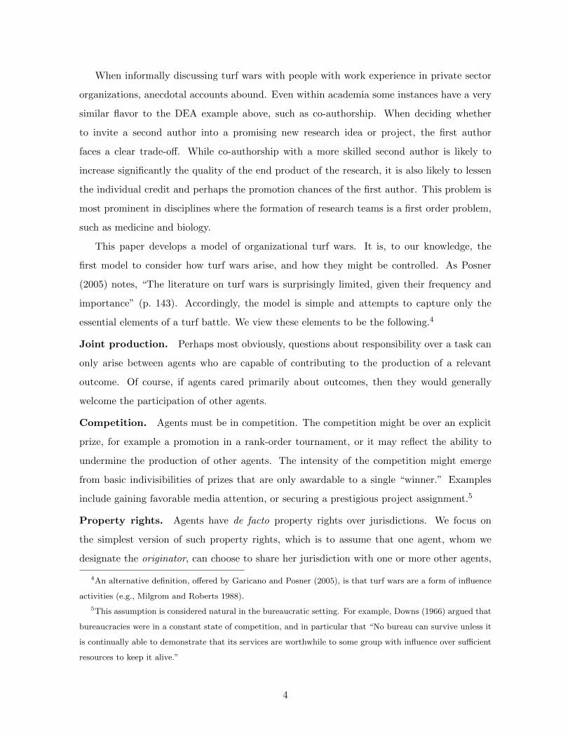
use the fact that all subjects participated in the four predicted outcomes, which allows us to

evaluate the effect the equilibrium predictions at the individual level. However, since subjects

repeatedly interacted with each other within matching groups, we construct our independent

observations by averaging the subjects’ behavior within each matching group. This procedure

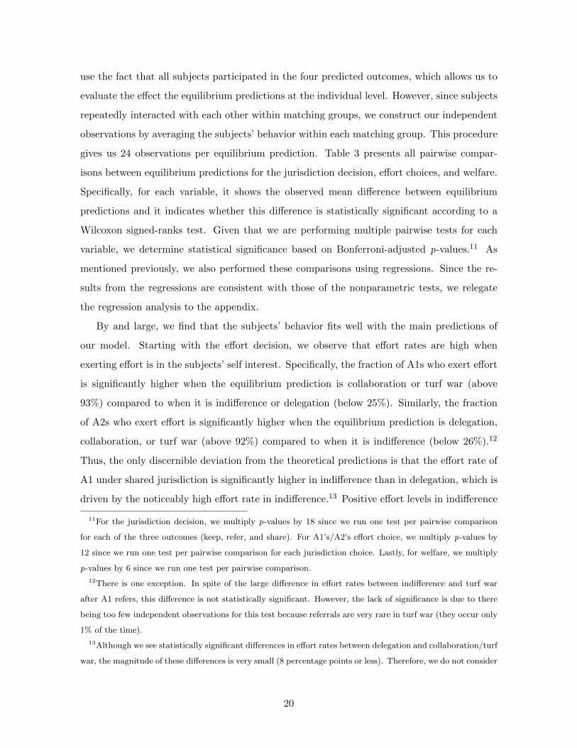
gives us 24 observations per equilibrium prediction. Table 3 presents all pairwise compar-

isons between equilibrium predictions for the jurisdiction decision, effort choices, and welfare.

Specifically, for each variable, it shows the observed mean difference between equilibrium

predictions and it indicates whether this difference is statistically significant according to a

Wilcoxon signed-ranks test. Given that we are performing multiple pairwise tests for each

variable, we determine statistical significance based on Bonferroni-adjusted p-values.11 As

mentioned previously, we also performed these comparisons using regressions. Since the re-

sults from the regressions are consistent with those of the nonparametric tests, we relegate

the regression analysis to the appendix.

By and large, we find that the subjects’ behavior fits well with the main predictions of

our model. Starting with the effort decision, we observe that effort rates are high when

exerting effort is in the subjects’ self interest. Specifically, the fraction of A1s who exert effort

is significantly higher when the equilibrium prediction is collaboration or turf war (above

93%) compared to when it is indifference or delegation (below 25%). Similarly, the fraction

of A2s who exert effort is significantly higher when the equilibrium prediction is delegation,

collaboration, or turf war (above 92%) compared to when it is indifference (below 26%).12

Thus, the only discernible deviation from the theoretical predictions is that the effort rate of

A1 under shared jurisdiction is significantly higher in indifference than in delegation, which is

driven by the noticeably high effort rate in indifference.13 Positive effort levels in indifference

11For the jurisdiction decision, we multiply p-values by 18 since we run one test per pairwise comparison

for each of the three outcomes (keep, refer, and share). For A1’s/A2’s effort choice, we multiply p-values by

12 since we run one test per pairwise comparison for each jurisdiction choice. Lastly, for welfare, we multiply

p-values by 6 since we run one test per pairwise comparison.

12There is one exception. In spite of the large difference in effort rates between indifference and turf war

after A1 refers, this difference is not statistically significant. However, the lack of significance is due to there

being too few independent observations for this test because referrals are very rare in turf war (they occur only

1% of the time).

13Although we see statistically significant differences in effort rates between delegation and collaboration/turf

war, the magnitude of these differences is very small (8 percentage points or less). Therefore, we do not consider

20

Tab

le3.

Ob

serv

ed

diff

ere

nces

inb

eh

avio

rd

ep

en

din

gon

equ

ilib

riu

mp

red

icti

on

s

Agent

Action

Treatmentcompa

risons

Ind

iffer

ence

Ind

iffer

ence

Ind

iffer

ence

Del

egati

on

Del

egati

on

Coll

ab

ora

tion

vs.

vs.

vs.

vs.

vs.

vs.

Del

egati

on

Coll

ab

ora

tion

Tu

rfw

ar

Coll

ab

ora

tion

Tu

rfw

ar

Tu

rfw

ar

A1

Kee

p0.

03

0.00

−0.7

8∗∗

−0.0

3∗∗

−0.8

1∗∗

−0.

78∗∗

Ref

er−

0.22∗∗

0.12∗∗

0.1

3∗∗

0.3

4∗∗

0.3

5∗∗

0.01

Sh

are

0.19∗∗

−0.

12∗∗

0.6

5∗∗

−0.3

1∗∗

0.46∗∗

0.77∗∗

Eff

ort

(aft

erke

ep)

−0.

08

−0.

87∗∗

−0.9

4∗∗

−0.7

9∗

−0.

86∗

−0.

07

Eff

ort

(aft

ersh

are)

0.21∗

∗−

0.74∗∗

−0.

72∗∗

−0.9

5∗∗

−0.

93∗∗

0.01

A2

Eff

ort

(aft

erre

fer)

−0.

80∗∗

−0.

83∗∗

−0.8

6−

0.0

3−

0.0

6−

0.03

Eff

ort

(aft

ersh

are)

−0.

66∗∗

−0.

73∗∗

−0.7

4∗∗

−0.0

7∗∗

−0.

08∗∗

−0.

01

Bot

hW

elfa

re−

0.26∗∗

−0.

70∗∗

−0.1

2∗∗

−0.4

3∗∗

0.1

4∗∗

0.58∗∗

Note

:M

ean

diff

eren

ces

inob

serv

edb

ehav

ior

bet

wee

neq

uil

ibri

um

pre

dic

tion

s.∗∗

an

d∗

ind

icate

stati

stic

al

sign

ifica

nce

at1%

and

5%ac

cord

ing

toW

ilco

xon

sign

ed-r

an

ks

test

su

sin

gm

atc

hin

g-g

rou

pm

ean

san

dB

on

ferr

on

i-ad

just

edp

-valu

es.

21

than in delegation are consistent with the large literature on cooperation in social dilemmas,

which shows that some individuals are willing to cooperate when everyone’s dominant strategy

is to defect (Fehr and Gachter 2000) but are less willing to do so if cooperation is in the

monetary interest of other players (e.g., see Reuben and Riedl 2009; Glockner et al. 2011).

In the preceding decision, we observe strong differences in A1’s jurisdiction decision de-

pending on the predicted equilibrium. Remarkably, the rate at which A1s keep jurisdiction

is less then 6% when the equilibrium prediction is delegation or collaboration, but it in-

creases significantly to 84% when the equilibrium prediction is a turf war. Contrary to the

model’s predictions, however, we observe that A1s choose to refer jurisdiction to A2s when the

equilibrium prediction is delegation resulting in significantly less sharing in delegation than in

collaboration. We will come back to this behavior when we analyze the individual treatments.

Finally, although the model does not make a prediction for the jurisdiction decision when the

equilibrium prediction is indifference, we observe that A1s choose to share jurisdiction most

of the time (80%). Note that sharing in this case is consistent with the fact that effort rates

are not exactly zero and are slightly higher when A1 shares.

Lastly, we observe that the total welfare in the experiment conforms with the predicted

comparative statics. Namely, welfare increases significantly as we move from indifference to

delegation and then to collaboration, but it subsequently decreases significantly when the

prediction becomes a turf war.14 In fact, we clearly observe the detrimental effect of turf wars

as total welfare is significantly lower when the equilibrium prediction is a turf war compared

to when it is delegation even though the players’ mean productivity is higher in the former

case.

Next, we take a look at behavior in the individual treatments. We provide a detailed sta-

tistical analysis based on both regressions and nonparametric tests in the appendix. Here, we

concentrate on the behavioral patterns observed above. Figure 4 presents the same statistics

as Figure 3 for each combination of β and θ1. On the whole, we do not find that behavior in

treatments with the same equilibrium prediction differ substantially from each other. There

are some differences, however, which we will highlight below.

them to be a substantial deviation from the theoretical predictions.

14Observed total welfare is close to the model’s point predictions: it is slightly higher if the equilibrium

prediction is indifference (0.19 vs. 0.00) or a turf war (0.31 vs. 0.23), and it is slightly lower if the prediction

is delegation (0.45 vs. 0.50) or collaboration (0.89 vs. 0.94).

22

Once again, let us start with the effort decision. We can see that, as predicted, the fraction

of A1s and A2s who exert effort increases with the amount of competition. Specifically, effort

rates are high, above 89%, when β is high enough to give subjects a monetary incentive to

exert effort (i.e., for β ≥ 0.50 if θi = 0.95 or β ≥ 0.80 if θi = 0.75), otherwise effort rates do

not exceed 48%. Figure 4 also reveals that the high effort rate observed when the equilibrium

prediction is indifference is driven by players with high productivity. This observation is

consistent with the literature on social dilemmas, which has documented that individuals are

more willing to cooperate when the benefits of doing so are high relative to the cost (e.g.,

Brandts and Schram 2001).

In the jurisdiction decision, we observe that increasing competition has a strong effect on

whether A1s keep jurisdiction to themselves, but only if A1 is of intermediate productivity

(θ1 = 0.75). The rate at which A1s with intermediate productivity keep jurisdiction is at

most 8% when β ≤ 0.80 but it rises to 84% when β = 0.95. By contrast, A1s with low or

high productivity (θ1 = 0.55 or θ1 = 0.95) keep jurisdiction at most 9% of the time at all four

values of β. As mentioned above, a behavior that is not in line with the model’s predictions

is the referral rate when the equilibrium prediction is delegation. We can see in Figure 4

that the high referral rate occurs in the two delegation treatments where β = 0.50. In other

words, in the two treatments where the difference between referring and sharing jurisdiction

is the lowest. Therefore, once again, deviations from the model’s predictions occur when such

deviations are not very costly. It is a common finding in experiments for deviations from Nash

equilibria to occur more often when they are less harmful. We would like to note, however, that

while such low-cost deviations can lead to substantial differences in behavior and welfare in

some games (see Goeree and Holt 2001), this is not the case in our model. More precisely, the

unexpectedly high effort and referral rates do not affect our model’s more notable implications

such as the nonlinear effect of competition and productivity on production and welfare.

Finally, consistent with the theoretical predictions, we can see that even though the in-

centive to provide effort increases with competition at all productivity levels, total welfare

does not. In particular, in pairs in which A1 is of intermediate productivity, welfare increases

as β goes from 0.15 to 0.80, but subsequently decreases when β reaches 0.95. In pairs where

A1 is of low or high productivity, welfare does not decrease as β increases. As a consequence,

pairs with an A1 with θ1 = 0.75 and β = 0.95 end up producing less than pairs with a less

productive A1 (θ1 = 0.55, as long as β ≥ 0.50).

23

0.0

0.2

0.4

0.6

0.8

1.0

0.0

0.2

0.4

0.6

0.8

1.0

0.0

0.2

0.4

0.6

0.8

1.0

β15 β50 β80 β95 β15 β50 β80 β95 β15 β50 β80 β95

Keep Refer Share

A1’s effort | Keep A1’s effort | Share

A2’s effort | Refer A2’s effort | Share Total welfare

θ55 θ75 θ95

Figure 4. Means of selected variables by treatment

Note: From the top-left to the bottom-right: the first three graphs depict the mean rate at

which A1 keeps, refers, or shares jurisdiction; the next four graphs depict the mean effort

rate of A1/A2 depending on the A1’s jurisdiction choice; and last graph depicts mean total

welfare as a fraction of maximum welfare (i.e., the sum of payoffs when both players have

high productivity, jurisdiction, and exert effort). Error bars correspond to 95% confidence

intervals.

In summary, our experimental results are in line with our model’s theoretical results. First,

we clearly observe how increasing the incentive to compete initially increases production

as it provides an incentive to exert effort. Second, we also observe that further increases

in competitive incentives can result in suboptimal jurisdiction decisions and a considerable

reduction of production (and welfare). Third, we find that such turf wars occur when the

productivity difference between A1 and A2 is neither too large nor too small.

24

3 Extensions

Here we discuss three interesting variations of the basic game, which are formally solved

in the appendix. Our objective is to show that the theoretical predictions from the basic

model are robust to small changes in payoff structure, effort assumptions, and informational

assumptions.

3.1 Fixed prize

A straightforward extension addresses environments where the competitive prize is a fixed

amount. This may be the case, for example, if agents compete for a promotion to a predeter-

mined office. The model with a fixed prize is identical to the basic model, with the exception

that the prize for victory is simply β instead of β(x1 + x2). We retain the assumption that

no prize is given when neither agent exerts effort.

In the second period, the effort decision is qualitatively similar to the one obtained in the

variable prize case. Following A1’s choice to share, Ai works when her counterpart works if

m(θ1 + θ2) + β ωi(θi, θ−i) − k ≥ mθ−i + β ωi(0, θ−i). Likewise, Ai works when her partner

does not work if mθi + β ωi(θi, 0) − k ≥ 0. As in the basic model, both of these expressions

evaluate to the same threshold value for θi, which we define as follows

θi ≥ θHf ≡k

m+ β2

. (8)

It is also straightforward to verify that when Ai’s partner does not work, then Ai will work

if θi exceeds the following threshold.

θi ≥ θLf ≡k − βm

. (9)

The thresholds θHf and θLf work analogously to the thresholds θH and θL in the basic

model. For θi < θLf , Ai exerts no effort, and for θi > θHf , Ai always exerts effort. For

θi ∈ (θLf , θHf ), Ai works only if she has sole jurisdiction. Again, each agent is more inclined to

work when she has sole jurisdiction as opposed to shared jurisdiction, since the latter entails

a positive probability of losing β even when the partner exerts no effort.

A1’s first period strategy anticipates A2’s effort response. The next proposition summa-

rizes outcomes and comparative statics for all combinations of θ1 and θ2. The result makes

use of the following notation. For θ1 ∈ (θLf , θHf ), A1 is indifferent between keeping and sharing

25

at the following threshold for θ1:

θ−f ≡k − β

2

m+ θ2

(1− β

2m

). (10)

It is straightforward to verify that θ−f > θLf . Next, for θ1 > θHf , A1 is indifferent between

keeping and sharing at the following threshold for θ1:

θ+f ≡ 1 + θ2

(1− 2m

β

). (11)

Proposition 3 (Outcomes under fixed prize)

(i) If θ2 ∈ (0, θLf ) then

indifference if θ1 < θLf

autarchy if θ1 > θLf .

(ii) If θ2 ∈ (θLf , θHf ) then

referral if θ1 <(θ2 + θLf

)autarchy∗ if θ1 >

(θ2 + θLf

).

(iii)If θ2 ∈ (θHf , 1) then

delegation∗ if θ1 < min{θ−f , θ

Hf }

turf war∗ if θ1 ∈(

min{θ−f , θHf },min{max{θ+f , θ

Hf }, 1}

)collaboration∗ if θ1 > max{θ+f , θ

Hf },

where (∗) denotes regions that may be empty.

The main findings are analogous to those of the basic model. For θ2 < θHf , A1s with

high productivity prefer autarchy, while those with low productivity prefer indifference or,

when A2 is willing to work under sole jurisdiction, referral. Sharing occurs only if θ2 > θHf ,

in which case turf wars occur for “intermediate” values of θ1: the originator chooses to keep

jurisdiction because sharing would greatly reduce her chances of receiving the prize to a high-

ability partner. By contrast, when the originator’s productivity is low enough to make her

either unwilling to exert effort or unlikely to win, the result is delegation. Finally, when the

originator’s productivity level guarantees a sufficiently high probability of winning the prize,

the result is collaboration.

The comparative statics on outcomes behave in an intuitive manner, and resemble those of

the basic model. When the value of the prize is high relative to the common value payoff (i.e.,

β > 2m), there is no collaboration. Higher values of β enlarge the set of θ1 values for which

there is a turf war and correspondingly reduce delegation. For β < 2m there is collaboration,

and collaboration is increasingly desirable to the originator as θ2 decreases. Finally, as k

26

Delegation

Collaboration

Turf war

0.0

0.2

0.4

0.6

0.8

1.0

θ1

0.0 0.2 0.4 0.6 0.8 1.0 β

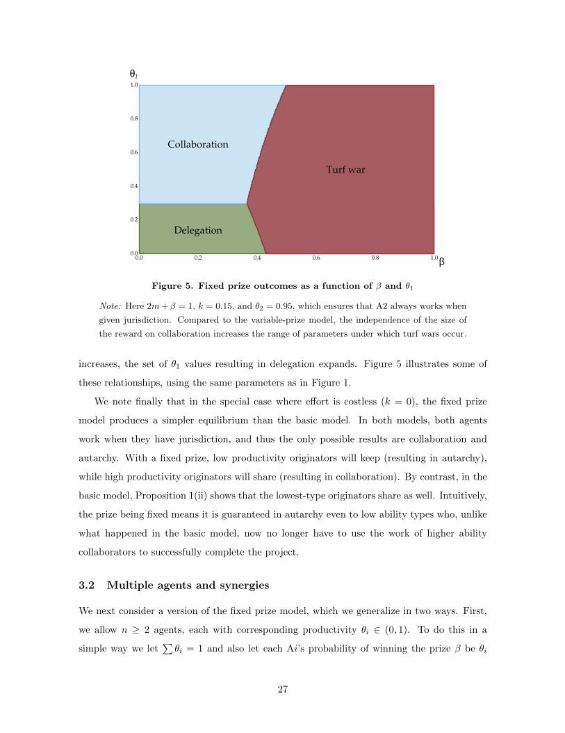
Figure 5. Fixed prize outcomes as a function of β and θ1

Note: Here 2m+ β = 1, k = 0.15, and θ2 = 0.95, which ensures that A2 always works when

given jurisdiction. Compared to the variable-prize model, the independence of the size of

the reward on collaboration increases the range of parameters under which turf wars occur.

increases, the set of θ1 values resulting in delegation expands. Figure 5 illustrates some of

these relationships, using the same parameters as in Figure 1.

We note finally that in the special case where effort is costless (k = 0), the fixed prize

model produces a simpler equilibrium than the basic model. In both models, both agents

work when they have jurisdiction, and thus the only possible results are collaboration and

autarchy. With a fixed prize, low productivity originators will keep (resulting in autarchy),

while high productivity originators will share (resulting in collaboration). By contrast, in the

basic model, Proposition 1(ii) shows that the lowest-type originators share as well. Intuitively,

the prize being fixed means it is guaranteed in autarchy even to low ability types who, unlike

what happened in the basic model, now no longer have to use the work of higher ability

collaborators to successfully complete the project.

3.2 Multiple agents and synergies

We next consider a version of the fixed prize model, which we generalize in two ways. First,

we allow n ≥ 2 agents, each with corresponding productivity θi ∈ (0, 1). To do this in a

simple way we let∑θi = 1 and also let each Ai’s probability of winning the prize β be θi

27

when all agents have jurisdiction. Second, we use the more general CES production function

for determining output x = (∑

i θρi )

1/ρ, where

∑i θi = 1 and ρ > 0. If ρ = 1 then abilities

are perfect substitutes. For ρ < 1 there are synergies in working together (the total ability

is larger than the sum of the abilities), and conversely for ρ > 1. For simplicity, we work

out the model without moral hazard (i.e., the case where k = 0), which implies that agents

automatically exert effort and the only possible outcomes are turf war and collaboration.

To start, consider the case where the sole originator, A1, can share with either all other

agents or none. Since there is no effort choice, the problem reduces to A1’s sharing decision

and the only possible outcomes are turf war and collaboration (i.e., not sharing is obviously

inefficient). Given sharing by A1, agent Ai’s expected utility can be written as

ui = m(∑

θρi

)1/ρ+ βθi.

Here ρ > 0 is the substitutability or complementarity of abilities. For example, if ρ = 1 then

abilities are perfect substitutes, for ρ < 1 there are synergies in working together (the total

ability is larger than the sum of the abilities), and conversely for ρ > 1. As in the basic fixed

prize, zero effort cost game, the originator’s utility from not sharing is simply mθ1 + β.

A1 shares if and only if

m

( n∑i=1

θρi

)1/ρ

− θ1

> β (1− θ1) .

It will then be convenient to express the condition for sharing as

A(θ1) ≡(∑n

i=1 θρi )

1/ρ − θ11− θ1

>β

m.

A(θ1) can be understood as a measure of the A1’s net gain from sharing.

As in the preceding analysis, we are mainly interested in seeing how the originator’s

productivity affects the propensity to share. Since productivity levels sum to a constant, the

results depend on how changes in θ1 affect θi for i 6= 1. One simple way to do this is to assign

non-negative linear “weights” to each player’s productivity parameter, of the following form:

θi = πi(1− θ1).

It is straightforward to derive each πi. Note that θ1 = 1 − θi/πi for each i 6= 1, which

implies that θi/πi is constant for all i 6= 1. Furthermore, to ensure that∑

i θi = 1, the weights

28

πi must satisfy∑

i 6=j πi = 1. This implies that for each i 6= 1,∑k 6=j

πk =∑k 6=j

θkθiπi = 1,

and therefore we have the following unique weights for each pair

πi =θi∑k 6=1 θk

.

This is simply agent i’s relative weight among the set of A2s. These weights imply that

as θ1 increases, the remaining θi’s must all shrink in proportion with their relative size. The

first result presents the basic comparative statics of the model.

Proposition 4 (Sharing with multiple agents and synergies)

(i) For any θ1 ∈ [0, 1), ρ Q 1 =⇒ dAdθ1R 0.

(ii) For any θ1 ∈ (0, 1), ρ Q 1 =⇒ A(θ1) R 1, and A(0) =

1 if n = 2

Q 1 if ρ R 1 if n > 2.

(iii) dAdρ < 0.

Part (i) of Proposition 4 shows how synergies and A1’s type matter for A1’s sharing

decision, and is the main point of comparison with the basic model. For ρ < 1 and β/m

sufficiently high, there is a “cutoff” value of θ1 above which A1 shares. This is consistent with

the basic model, where the most productive A1s share, conditional upon being willing to work.

From a welfare perspective this is a bad result, as it would be better for lower productivity

A1s to share. For ρ > 1 and β/m sufficiently low, however, the pattern is reversed: there is

another cutoff value of θ1 below which A1 shares. Low type A1s also shared in some cases of

the basic model, but always along with high types. Interestingly, in the linear case (ρ = 1)

the propensity to share does not depend on θ1, and depends only on the agents’ relative

policy motivation. Thus with the caveat that the results are not directly comparable with

those of the basic model because the values of θi are not independent, the result shows that

the pattern of collaboration can be at least somewhat sensitive to the presence of production

synergies. Part (ii) shows how the critical value for β/m depends on synergies. For n > 2,

values of β/m very close to 1 can make sharing either optimal for all θ (ρ < 1) or not optimal

for all θ (ρ > 1). Part (iii) simply establishes the intuitive result that the benefit of sharing is

decreasing in ρ (i.e., increasing in synergy). Thus, the greater the synergy, the more inclined

A1 will be to share.

29

We finally consider what would happen if the originator could choose the set of agents

she shares with. There are two cases. First, suppose that A1 can share the task with only

one additional agent. As the probability of victory conditional upon sharing with Ak is

θ1/(θ1 + θk), A1 would be willing to add agent Ak if

m(θρ1 + θρk

)1/ρ+ β

θ1θ1 + θk

> mθ1 + β(θρ1 + θρk

)1/ρ − θ1 >θk

θ1 + θk

(β

m

).

Note that this expression is identical to that of the two-agent case when θ1 + θk = 1.

There are two effects of increasing θk: increasing the probability of a successful outcome, and

decreasing the probability of winning the award. The preceding expression can be rewritten

as follows:

A(θ1, θk) = (θ1 + θk)

[((θ1θk

)ρ+ 1

)1/ρ

− θ1θk

]>β

m. (12)

This expression implies that holding θ1/θk constant, sharing becomes harder as θ1 + θk

shrinks. This happens because the contribution of sharing toward the collective outcome

becomes smaller, while the probability of winning the prize remains the same. Likewise,

holding θ1 + θk constant, sharing becomes easier (harder) as θ1 increases if ρ < (>) 1. The

next comment characterizes A1’s choice of a single partner.

Comment 1 (Optimal partner)

For potential partner Ak:

(i) If ρ < 1, ∂A∂θ1

> 0. If ρ > 1, ∂A∂θ1

> 0 if θ1 ≤ θk and ρ sufficiently large; limρ→∞∂A∂θ1

= 0

if θ1 > θk.

(ii) If ρ > 1, ∂A∂θk

> 0. If ρ < 1, ∂A∂θk

> 0 if θ1 ≤ θk; limρ→∞∂A∂θk

< 0 if θ1 > θk.

Part (i) considers A1’s productivity. When ρ < 1 (i.e., there are synergies), high pro-

ductivity A1s will be more inclined to share with a given partner. The results are weaker

when ρ > 1 but A1s with high productivity will often do better in a partnership than those

with low productivity. Part (ii) considers the more interesting question of whom A1 would

choose. Often more productive partners are preferred. Interestingly, when ρ > 1 A1 prefers

partners with high productivity because the expected loss in the victory bonus is now offset by

productivity gains. This is also true when ρ < 1 and potential partners are more productive

than A1. The relationship may be reversed if potential partners are less productive than A1.

30

Next, consider a second case where the originator can choose t agents to partner with, but

all agents are identical (θi = θ). Thus, the originator’s objective is

L(t) ≡ m(t

(1

n

)ρ)1/ρ

+β

t. (13)

where t ∈ {1, . . . , n}.

This objective is considerably simpler than that with heterogeneous agents, and so it is

straightforward to derive the following comment.

Comment 2 (Optimal number of homogeneous partners)

If βm ≥

n1/ρ−1n−1 , then t∗ = 1; otherwise, t∗ = n.

As intuition would suggest, when the bonus from victory is relatively important, then

there is less sharing. Somewhat more interestingly, there is never an interior solution, and so

the originator will share with either no agents or all agents.

3.3 Incomplete information

We now discuss a version of the game in which each agent is uncertain of the other’s productiv-

ity. Specifically, suppose that θi ∼ U [0, 1] for agent Ai. In this environment, the originator’s

sharing decision serves a signal of the originator’s productivity.

We retain the fixed reward and make three other modifications to further simplify the

analysis. First, we do not consider referrals. Second, A1 is assumed always to work, with her

effort level denoted simply by e. Conditional upon Ai having jurisdiction, output xi is then

x1 = θ1 ∼ U [0, 1]

x2 =

θ2 ∼ U [0, 1] if e = 1

0 if e = 0.

Third, uncertainty over productivity eliminates the need for ε in the basic model; thus, agent

Ai wins the prize β if xi > x−i. The model might therefore describe a situation in which

the originator is required to work on a project, but still decides whether to share jurisdiction

or not. We characterize a perfect Bayesian equilibrium of this game. As the subsequent

derivations show, there is essentially a unique equilibrium. Formally, strategies consist of

A1’s sharing choice s ∈ {share, keep} and A2’s effort level e ∈ {0, 1} conditional upon having

jurisdiction. A2 also has posterior beliefs over θ1 given A1’s sharing decision, denoted ρ :

31

{share, keep} → P, where P is the set of measurable subsets of [0, 1]. These beliefs are

consistent with Bayes’ rule along the equilibrium path. An out of equilibrium information set

can only be encountered if A1 shares when she was not expected to do so. In these cases,

we simply assume that A2’s beliefs are concentrated on θ1 = 1. Although the equilibrium

does not require such extreme beliefs, this designates the type that would benefit most from

sharing, since she would win with probability one.

We begin by considering the subgame following A1’s choice to share, where agent A2 has

posterior beliefs about A1’s productivity that are uniformly distributed on the interval (θ, θ].

While this is not a fully general treatment of A2’s possible beliefs, we will subsequently argue

that A1’s sharing strategies are monotonic and therefore must take this form in equilibrium.

A2 works if

m (E[θ1| share] + θ2)− k + β ω(θ, θ, θ2, e) > mE[θ1| share]. (14)

Here ω(θ, θ, θ2, e) represents the probability that A2 wins. The uniform distribution implies

that

ω(θ, θ, θ2, 1) =

0 if θ2 < θ

θ2−θθ−θ if θ2 ∈ [θ, θ]

1 if θ2 > θ,

and expression (14) simplifies to

mθ2 + β ω(θ, θ, θ2, e) > k.

As intuition would suggest, working becomes more attractive to A2 as m, θ2 and β increase,

and less attractive as k increases. The expression implies that for any (θ, θ], there is a unique

type θ2 such that higher productivity types work and lower productivity types shirk. This

type is given by

θ2 =

km if θ ≥ k

m

min{

1, k(θ−θ)+βθm(θ−θ)+β

}if θ < k

m .(15)

The first line of (15) gives a corner case where A2 is indifferent between working and not

even though she expects to lose β with certainty. Thus, strong policy motivations alone can

induce some types to work even when they expect to lose with certainty. The second line

gives the interior case where the indifferent A2 expects to win with some probability. Because

this set of types necessarily hits a corner at 1, this threshold must be weakly increasing in θ.

32

Reducing the set of sharing originator types (i.e., increasing θ) therefore does not expand the

set of partner types willing to work.

Given θ2, the probability that A2 will work given (θ, θ] is

φ(θ, θ) = 1− θ2. (16)

And given θ1, the probability that A2 wins conditional upon working is

ξ(θ1) =

1 if θ1 ≤ θ21−θ11−θ2

if θ1 ≥ θ2.(17)

Note that if θ1 < θ2, then the probability of A1 winning is zero.

We can now characterize A1’s sharing decision. Suppose that in equilibrium, the set of

sharing originators is (θ, θ]. Then A1 shares if

m

(θ1 + φ(θ, θ)

θ2 + 1

2

)+ (1− φ(θ, θ)ξ(θ1))β > mθ1 + β (18)

Simplifying, A1 shares if φ(θ, θ) > 0 and

m(θ2 + 1)

2− ξ(θ1)β > 0 (19)

There are two notable facts about this expression. First, it is independent of φ(·) when

φ(·) 6= 0. Second, it does not depend on the functional form of ξ(·); i.e., it applies to any

measurable sharing strategy on [0, 1]. This implies an important monotonicity feature of

sharing in equilibrium. If any type θ′1 shares in equilibrium, then all higher types will also be

willing to share. To see why, suppose that some type θ′′1 > θ′1 does not share. By sharing out

of equilibrium, she would not affect A2’s strategy, and so would only affect A2’s chances of

winning. Thus, type θ′′1 would automatically satisfy (19) if type θ′1 does.

The immediate consequence of the monotonicity of sharing incentives is that when sharing

occurs, the set of sharing types is simply (θ, 1]. The final step in deriving the equilibrium is

then to characterize θ. At an interior solution, this is the (unique) value of θ1 that satisfies

(19) with equality. Higher values of θ imply lower levels of sharing. There are also corner

solutions, where either no types or all types share.

Our next result describes the outcomes of the incomplete information game. Note that a

difference between these results and those of preceding versions of the game is that collabo-

ration and turf wars can only be probabilistic as they depending on the specific realization

33

of θ2. That is, a set of sufficiently low types of A2 will find the utility gains from working to

not warrant the effort. Thus, except in the limiting case where full sharing occurs and k → 0,

there is no equilibrium in which A2 always works. We therefore label outcomes where A1

shares and A2 works with positive probability as “possible collaboration” and those where

A1 does not share but A2 would work with positive probability as a “possible turf war.”

Proposition 5 (Outcomes under incomplete information)

(i) (Indifference) If β ≤ k −m, then the outcome is indifference.

(ii) (Possible turf war) If β > k −m and m < min{k, β}, then A1 keeps for all θ1.

(iii) (Possible collaboration) If β ∈(k −m, −m+

√m2+8m(k+m)

4

), then A1 shares for all θ1.

(iv) (Possible collaboration and turf war) If the conditions of parts (i)-(iii) are not met, then

the set of sharing types is (θ∗, 1], where

θ∗ =

m(k−β+m)−2β2

m(k−3β+m) if m ≤ k and m ≥ β, or m > k and k+m2 > β

1− m(1−(k/m)2)2β otherwise.

Proposition 5 provides some basic intuitions about the effects of turf battles on sharing.

Part (i) shows that the conditions generating indifference—low β, high k, and low m—are

similar to those in Proposition 1. Parts (ii) and (iii) are the corner cases; in the former,

autarchy is always the result because all A1 types play keep because β is sufficiently high.

In the latter, all types of A1 share because β is moderate and m is high. Finally, part (iv)

is the interior solution, where autarchy results for low values of θ1 and possible collaboration

for higher values.

The role of β in the incomplete information game resembles that of the basic game. Clearly,

extreme values of β are undesirable from the perspective of maximizing joint production; very

low values provide too little incentive to work, and very high values provide too little incentive

to share. Focusing on intermediate values (i.e., parts (iii) and (iv) of Proposition 5), increasing

β limits A1’s propensity to share. For low values of β in this region there is full sharing. The

following comment establishes that the set of types that share contracts as β increases.

Comment 3 (Comparative Statics)

θ∗ is increasing in β.

These results show that despite numerous differences across models, two main intuitions

carry over from the basic model. First, high levels of competition will inhibit sharing and

34

collaboration. Second, conditional upon being willing to work, the highest type originators

will share in equilibrium. This prediction is also consistent with the “synergies” case (ρ < 1)

case of the no-effort model. As with the other models, equilibrium sharing behavior is in some

sense undesirable, as a hypothetical principal or society would prefer that lower types share.

4 Discussion

The goal of this paper is largely positive: we attempt to formalize the popular notion of a turf

war. As we argue, the minimal necessary components of a turf war are joint production, com-

petition, and property rights over jurisdiction. From this starting point, our model produces

a unique equilibrium in which high-productivity originators share and high-productivity part-

ners exert effort. One implication is that turf battles hurt most when collaboration is most

needed; that is, when originators have moderate productivity. Perhaps most prominently, it

shows that the reward from competition, β, can both help and hurt collaboration. While

competition always mitigates moral hazard and free riding by inducing effort, high levels of

competition can encourage originators to “go it alone.”

Despite their ubiquity, turf wars are difficult to observe directly. In fact, inefficient lack of

cooperation is present and most prominent precisely when the failure to share a task is hard

to monitor and hence discipline directly. Our experiment therefore sought to test the model’s

predictions about originator sharing behavior when there is an able partner willing to work.

Consistent with a host of previous results, subjects cooperated somewhat more often than

predicted by the model. Yet the main predictions about the role of competitive versus policy-

motivated incentives are supported, and in particular there is support for the non-monotonic

effects of competitive rewards on collaboration.

While we view our basic model as capturing a necessary and sufficient condition for turf

wars, other factors may also matter. Agents are limited by being unable to strike bargains to

divide the surplus with either each other or the principal. We also do not consider organiza-

tional solutions such as the selection of agent types, or incentives provided through oversight

or contracts. Yet, the model allows us to speculate on some possible remedies. For example,

a principal could use a performance cutoff below which β is not awarded to any agent. This

scheme might correspond to an organization’s implicit threat to fill a higher position with an

outsider rather than promoting from within. This might produce collaboration by reducing

35

the payoff from autarchy, but it may also reduce the incentive of certain agent types to work.

Another important question concerns the way in which effort is aggregated. In our game

theoretic model, outputs are perfect substitutes. However, our decision theoretic extension

suggests the possibility that returns to scale and complementarities might affect sharing pat-

terns in a way that our other extensions did not. In an environment with rapidly diminishing

returns to collaborative effort, a hypothetical principal might actually want autarchy.

References

Alonso, R., Dessein, W., and Matouschek, N. (2008). When does coordination require cen-

tralization? American Economic Review, 98(1):145–179.

Austen-Smith, D. and Riker, W. (1987). Asymmetric information and the coherence of legis-

lation. American Political Science Review, 81(3):897–918.

Baccara, M. and Razin, R. (2007). Bargaining over new ideas: The distribution of rents and

the stability of innovative firms. Journal of the European Economic Association, 5(6):1095–

1129.

Brandts, J. and Schram, A. (2001). Cooperation and noise in public goods experiments:

Applying the contribution function approach. Journal of Public Economics, 79(2):399–427.

Camera, G. and Casari, M. (2009). Cooperation among strangers under the shadow of the

future. American Economic Review, 99(3):979–1005.

Chen, K.-P. (2003). Sabotage in promotion tournaments. Journal of Law, Economics, and

Organization, 19(1):119–140.

Chen, Y. and Ledyard, J. O. (2008). Mechanism design experiments. In Durlauf, S. N. and

Blume, L. E., editors, The New Palgrave Dictionary of Economics. Palgrave Macmillan,

Basingstoke.

Creane, A. (1995). Endogenous learning, learning by doing and information sharing. Inter-

national Economic Review, 36(4):985–1002.

Dechenaux, E., Kovenock, D., and Sheremeta, R. M. (2012). A survey of experimental research

on contests, all-pay auctions and tournaments. Economic science institute working paper

12-22, Chapman University.

Dessein, W., Garicano, L., and Gertner, R. (2010). Organizing for synergies. American

Economic Journal: Microeconomics, 2(4):77–114.

36

Downs, A. (1966). Inside Bureaucracy. Little, Brown, Boston, MA.

Falk, A., Fehr, E., and Huffman, D. (2008). The power and limits of tournament incentives.

Discussion paper, University of Zurich.

Fehr, E. and Gachter, S. (2000). Fairness and retaliation: The economics of reciprocity.

Journal of Economic Perspectives, 14(3):159–182.

Fischbacher, U. (2007). z-Tree: Zurich toolbox for ready-made economic experiments. Ex-

perimental Economics, 10(2):171–178.

Gal-Or, E. (1985). Information sharing in oligopoly. Econometrica, 53(2):329–343.

Garicano, L. and Posner, R. A. (2005). Intelligence failures: An organizational economics

perspective. Journal of Economic Perspectives, 19(4):151–170.

Garicano, L. and Santos, T. (2004). Referrals. American Economic Review, 94(3):499–525.

Gates, R. M. (1987). The cia and american foreign policy. Foreign Affairs, 66(2):215–230.

Glockner, A., Irlenbusch, B., Kube, S., Nicklisch, A., and Normann, H.-T. (2011). Leading

with(out) sacrifice? a public-goods experiment with a privileged player. Economic Inquiry,

49(2):591–597.

Goeree, J. K. and Holt, C. A. (1999). Stochastic game theory: For playing games, not just

for doing theory. Proceedings of the National Academy of Sciences, 96(19):10564–10567.

Goeree, J. K. and Holt, C. A. (2001). Ten little treasures of game theory and ten intuitive

contradictions. American Economic Review, 91(5):1402–1422.

Greiner, B. (2004). The online recruitment system ORSEE 2.0 – a guide for the organization

of experiments in economics. Working paper series in economics 10, University of Cologne.

Harbring, C. and Irlenbusch, B. (2005). Incentives in tournaments with endogenous prize

selection incentives in tournaments. Journal of Institutional and Theoretical Economics,

161(4):636.

Harbring, C. and Irlenbusch, B. (2011). Sabotage in tournaments: Evidence from a laboratory

experiment. Management Science, 57(4):611–627.

Hoffman, B. (2012). American Icon: Alan Mulally and the Fight to Save Ford Motor Company.

Crown Publishing, New York, NY.

Holmstrom, B. and Milgrom, P. (1990). Regulating trade among agents. Journal of Institu-

tional and Theoretical Economics, 146(1):85–105.

Institute of Medicine (2001). Crossing the quality chasm: A new health system for the 21st

century. National Academy Press, Washington, DC.

37

Itoh, H. (1991). Incentives to help in multi-agent situations. Econometrica, 59(3):611–636.

King, D. C. (1994). The nature of congressional committee jurisdictions. American Political

Science Review, 88(1):48–62.

King, D. C. (1997). Turf Wars: How Congressional Committees Claim Jurisdiction. Univer-

sity of Chicago Press, Chicago, IL.

Konrad, K. (2000). Sabotage in rent-seeking contests. Journal of Law, Economics, and

Organization, 16(1):155–165.

Lazear, E. P. (1989). Pay equality and industrial politics. Journal of Political Economy1,

97(3):561–580.

Lederman, G. N. (1999). Reorganizing the Joint Chiefs of Staff. Greenwood Press, Westport,

CT.

Lee, T. H. and Mongan, J. J. (2009). Chaos and Organization in Health Care. MIT Press,

Cambridge, MA.

Markussen, T., Reuben, E., and Tyran, J.-R. (2014). Competition, cooperation and collective

choice. The Economic Journal, 124(574):F163–F195.

Marx, L. M. and Squintani, F. (2009). Individual accountability in teams. Journal of Economic

Behavior & Organization, 72(1):260–273.

Medicare Payment Advisory Commission (2008). Report to Congress: Reforming the delivery

system. MedPAC, Washington, DC.

Milgrom, P. and Roberts, J. (1988). An economic approach to influence activities in organi-

zations. American Journal of Sociology, 94(1):154–179.

Modica, S. (2010). Open source without free riding. Mimeo, University of Palermo.

Nalbantian, H. R. and Schotter, A. (1997). Productivity under group incentives: An experi-

mental study. American Economic Review, 87(3):314–341.

National Commission on Terrorist Attacks (2004). The 9/11 Commission Report: Final

Report of the National Commission on Terrorist Attacks Upon the United States. W. W.

Norton & Company, New York, NY.

Okuno-Fujiwara, M., Postlewaite, A., and Suzumura, K. (1990). Strategic information reve-

lation. Review of Economic Studies, 57(1):25–47.

Posner, R. A. (2005). Preventing Surprise Attacks: Intelligence Reform in the Wake of 9/11.

Rowman & Littlefield, Stanford, CA.

Raith, M. (1996). A general model of information sharing in oligopoly. Journal of Economic

38

Theory, 71(1):260–288.

Reuben, E. and Riedl, A. (2009). Public goods provision and sanctioning in privileged groups.

Journal of Conflict Resolution, 53(1):72–93.

Stein, J. C. (2008). Conversations among competitors. American Economic Review,

98(5):2150–2162.

Tan, J. H. and Bolle, F. (2007). Team competition and the public goods game. Economics

Letters, 96(1):133–139.

Wilson, J. Q. (1978). The Investigators. Basic Books, New York, NY.

Wilson, J. Q. (2000). Bureaucracy: What Government Agencies Do and why They Do it.

Basic Books, New York, NY.

A Proofs

Proof of Lemma 1

We can rewrite

θH ≡−(m+ β

2

)+

√(m+ 3

2β)2

+ 2β (k − (m+ β))

β

It is then easily verified that k = m+ β iff θL = θH = 1, and k = 0 iff θL = θH = 0. The rest

is straightforward, as squaring both sides we obtain.

θH ≡−(m+ β

2

)+√

(m+ β2 )2 + 2βk

β>

k

m+ β≡ θ√(

m+β

2

)2

+ 2βk >kβ

m+ β+

(m+

β

2

)1 >

k

m+ β

Since k < m+ β, we have 0 < θL < θH < 1 �

Proof of Proposition 1

(i) and (ii) are derived in the text. For (iii), A2 always works as θ2 ∈ (θH , 1), so we have three

cases.

39

1. For θ1 ∈ (0, θL), A1 does not work. Since A2 works if she has jurisdiction, A1 re-

ceives zero from keeping and strictly positive utility from sharing. Thus the outcome is

delegation.

2. For θ1 ∈ (θH , 1) A1 always works and prefers keep (resulting in autarchy) over share

(resulting in collaboration) if

m(θ1 + θ2) + β(θ1 + θ2)ω1(θ1, θ2)− k < (m+ β)θ1 − k (20)

βθ21 − βθ1 + βθ2(1− θ2) + 2mθ2 < 0 (21)

The solutions (θ−, θ+) to (21) for θ1 are given by (6). Hence, if θ1 < θ− or θ1 > θ+,

then A1 shares. If θ1 ∈ (θ−, θ+) then A1 keeps. If θ− and θ+ are not real-valued, then

A1 shares.

3. For θ1 ∈ (θL, θH), A1 prefers share (resulting in delegation) to keep (resulting in

autarchy) if

mθ2 + βθ2 ω1(0, θ2) ≥ (m+ β)θ1 − k

θ1 ≤ θ ≡mθ2 + βθ2

1−θ22 + k

m+ β(22)

Since θ > θL always, this case breaks into two subcases:

3a. θ > θH , so θ is irrelevant: A1 delegates always in this region, hence at θ1 = θH A1,

by definition indifferent between collaboration and delegation, prefers either over

autarchy. If either θ− and θ+ are not real-valued, or θ+ < θH , then A1 does not

choose keep for any θ1 > θH . Combining the previous cases, the outcomes aredelegation if θ1 ∈

(0, θL

)delegation if θ1 ∈

(θL, θH

)collaboration if θ1 ∈

(θH , 1

).

And when θ− and θ+ are real-valued and θ+ > θH we have

delegation if θ1 ∈(0, θL

)delegation if θ1 ∈

(θL, θH

)collaboration if θ1 ∈

(θH , θ−

)autarchy (turf war) if θ1 ∈ (θ−, θ+)

collaboration if θ1 ∈ (θ+, 1) .

40

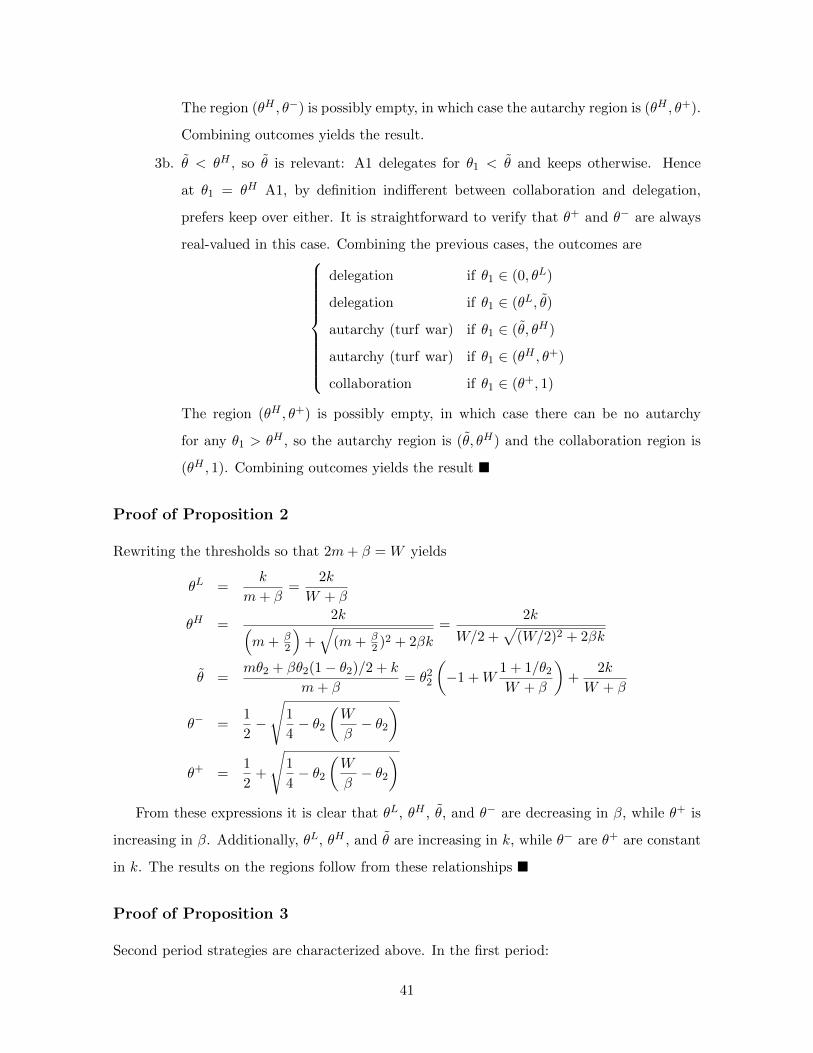
The region (θH , θ−) is possibly empty, in which case the autarchy region is (θH , θ+).

Combining outcomes yields the result.

3b. θ < θH , so θ is relevant: A1 delegates for θ1 < θ and keeps otherwise. Hence

at θ1 = θH A1, by definition indifferent between collaboration and delegation,

prefers keep over either. It is straightforward to verify that θ+ and θ− are always

real-valued in this case. Combining the previous cases, the outcomes are

delegation if θ1 ∈ (0, θL)

delegation if θ1 ∈ (θL, θ)

autarchy (turf war) if θ1 ∈ (θ, θH)

autarchy (turf war) if θ1 ∈ (θH , θ+)

collaboration if θ1 ∈ (θ+, 1)

The region (θH , θ+) is possibly empty, in which case there can be no autarchy

for any θ1 > θH , so the autarchy region is (θ, θH) and the collaboration region is

(θH , 1). Combining outcomes yields the result �

Proof of Proposition 2

Rewriting the thresholds so that 2m+ β = W yields

θL =k

m+ β=

2k

W + β

θH =2k(

m+ β2

)+√

(m+ β2 )2 + 2βk

=2k

W/2 +√

(W/2)2 + 2βk

θ =mθ2 + βθ2(1− θ2)/2 + k

m+ β= θ22

(−1 +W

1 + 1/θ2W + β

)+

2k

W + β

θ− =1

2−

√1

4− θ2

(W

β− θ2

)

θ+ =1

2+

√1

4− θ2

(W

β− θ2

)From these expressions it is clear that θL, θH , θ, and θ− are decreasing in β, while θ+ is

increasing in β. Additionally, θL, θH , and θ are increasing in k, while θ− are θ+ are constant

in k. The results on the regions follow from these relationships �

Proof of Proposition 3

Second period strategies are characterized above. In the first period:

41

(i) When θ2 ∈ (0, θLf ), A1 anticipates no effort from A2. A1 therefore works if θ1 > θLf

(resulting in indifference), and does not work otherwise (resulting in autarchy).

(ii) When θ2 ∈ (θLf , θHf ), sharing results in no effort by A2. Thus, A1 keeps if she prefers to

work herself, and refers if she prefers that A2 work alone, or mθ1 + β − k > mθ2. This

reduces to θ1 > θ2 + θLf . Thus, higher values of θ1 result in autarchy and lower values

result in referral.

(iii) When θ2 > θHf , since A2 is guaranteed to work, delegation yields a higher payoff than

referral. A1 therefore effectively decides over turf war, delegation, and collaboration, as

follows. For θ1 < θLf , A1 exerts no effort and delegation is clearly her most preferred

outcome; thus, she shares. For θ1 ∈ (θLf , θHf ), A1 exerts no effort when sharing. She then

prefers keeping to sharing when mθ1 +β− k > mθ2 +βω(0, θ2), or θ1 > θ−f . Combining

the subcases where θ1 < θHf , A1 shares for all θ1 < min{θ−f , θHf }, and keeps otherwise.

Finally, for θ1 > θHf , A1 exerts effort when sharing. She the prefers sharing to keeping

when m(θ1 + θ2) + βω(θ1, θ2)− k > mθ1 + β − k, or θ1 > θ+f . Combining the outcomes

from these regions produces the result �

Proof of Proposition 4

(i) Letting k1 = θ1/(1− θ1), this gives us:

A(θ1) =

(θρ1 +

∑i 6=1(πi(1− θ1))ρ

)1/ρ− θ1

1− θ1

=

kρ1 +∑i 6=1

(πi)ρ

1/ρ

− k1.

A(θ1) has the same sign as dAdk1

. The derivative with respect to k1 is

dA

dk1=

kρ1 +∑i 6=1

(πi)ρ

1−ρρ

kρ−11 − 1

=

1 + k−ρ1

∑i 6=1

(πi)ρ

1−ρρ

− 1,

which is positive (zero) (negative) if

1− ρρ

ln

1 + k−ρ1

∑i 6=1

(πi)ρ

> (=)(<) 0.

42

Since the term in parentheses is greater than 1, dAdk1

> (=)(<) 0 if ρ < (=)(<) 1.

(ii) Note first that

A(0) =

∑i 6=1

(πi)ρ

1/ρ

.

For n = 2, there is only one term in the summation, and πi = 1, so A(0) = 1. For

n > 2, since∑

i 6=1 πi = 1, it is clear that A(0) > (=)(<) 1 if ρ < (=)(>) 1. Finally, since

A′(θ1) > (=)(<) 0 for ρ < (=)(>) 1, we have A(θ1) > (=)(<) 1 when ρ < (=)(>) 1 for

θ1 > 0.

(iii) Let A(ρ) =(kρ1 +

∑i 6=1(πi)

ρ)1/ρ

, which has the same derivative as A(·) with respect to

ρ. Differentiating A(θ1) with respect to ρ, we obtain

1

A

dA

dρ=

1

ρ

kρ1 ln k1 +∑

i 6=1(πi)ρ lnπi

kρ1 +∑

i 6=1(πi)ρ

− 1

ρ2ln

kρ1 +∑i 6=1

(πi)ρ

.

Observe that A(ρ) > 0 for all ρ, and therefore dAdρ is negative if

kρ1 ln k1 +∑

i 6=1(πi)ρ lnπi

kρ1 +∑

i 6=1(πi)ρ

<1

ρln

kρ1 +∑i 6=1

(πi)ρ

.

Since πi > 0 for all i and lnπi < 0, the left-hand side of the expression above is strictly

less than ln k1. And since πi > 0 for all i, the right-hand side is strictly greater than

ln k1, thus establishing the result �

Proof of Comment 1

(i) As derived in the proof of Proposition 4, the bracketed expression in (12) is positive and

increasing in θ1 if ρ < 1. It follows that A(θ1, θk) is increasing in θ1 if ρ ≤ 1. For ρ > 1,

we differentiate with respect to θ1, and so ∂A∂θ1

< (>) 0 if

(θ1 + θk)

[((θ1θk

)ρ+ 1

)1/ρ−1(θ1θk

)ρ−1 1

θk− 1

θk

]+

((θ1θk

)ρ+ 1

)1/ρ

− θ1θk

< (>) 0.

Following the proof of Proposition 4, the bracketed expression is negative for ρ > 1,

while((

θ1θk

)ρ+ 1)1/ρ

− θ1θk

is positive. Letting k = θ1/θk and simplifying, we have

43

∂A∂θ1

< (>) 0 if1

(kρ + 1)1−1/ρ− 2k + 1

2kρ + kρ−1 + 1< (>) 0.

There are two cases. First, suppose k ≤ 1 (i.e., θ1 < θk). Since (kρ + 1)1/ρ−1 ≤ 1, it

follows that dAdθ1

< 0 if: 2kρ + kρ−1 < 2k, or kρ−1 < 2k/(2k+ 1). This is clearly satisfied

for ρ sufficiently large. Second, suppose k > 1. The limits of both fractions in the above

expression as ρ→∞ are clearly 0. Thus limρ→∞∂A∂θ1

= 0.

(ii) As derived in the proof of Proposition 4, the bracketed expression in (12) is positive and

increasing in θk if ρ > 1. It follows that A(θ1, θk) is increasing in θk if ρ ≥ 1. For ρ < 1,

we differentiate with respect to θk and substitute k = θ1/θk:, which gives

∂A

∂θk= (θ1 + θk)

[−((

θ1θk

)ρ+ 1

)1/ρ−1(

θρ1θρ+1k

)+θ1θ2k

]+

((θ1θk

)ρ+ 1

)1/ρ

− θ1θk

= k2 − (kρ + 1)1/ρ−1 kρ(k + 1) + (kρ + 1)1/ρ .

Thus ∂A∂θk

> (<) 0 if

k2 > (<) (kρ + 1)1/ρ[kρ(k + 1)

kρ + 1− 1

].

There are two cases. First, suppose k ≤ 1. Then ∂A∂θk

> 0 if kρ(k+1) ≤ kρ+1, or kρ+1 ≤

1, which holds for any ρ > 0. Second, suppose k > 1. Since limρ→∞(kρ + 1)1/ρ = k,

we have limρ→∞∂A∂θk

< 0 if limρ→∞kρ(k+1)kρ+1 > k + 1. Applying L’Hopital’s Rule yields

limρ→∞kρ(k+1)kρ+1 = (k+1)kρ ln k+kρ

kρ ln k = k + 1 + 1ln k , thus proving the result �

Proof of Comment 2

We first give the condition under which A1 prefers 1 partner to n partners. This is the case if

m

n+ β ≥ mn1/ρ−1 +

β

n

β

m≥ n1/ρ − 1

n− 1. (23)

Next we derive conditions under which A1’s objective is either strictly increasing or de-

creasing. Differentiating the objective L(t) (see (13)) yields L′(t) = mt1/ρ−1/(nρ) − βt−2.

This implies that L′(1) = m/(nρ) − β, which is positive if β/m < 1/(nρ). Note also that

L′(t) > 0 for all t ∈ [1, n] if mt1/ρ+1/(nρ)− β > 0. Since this expression is increasing in t, it

44

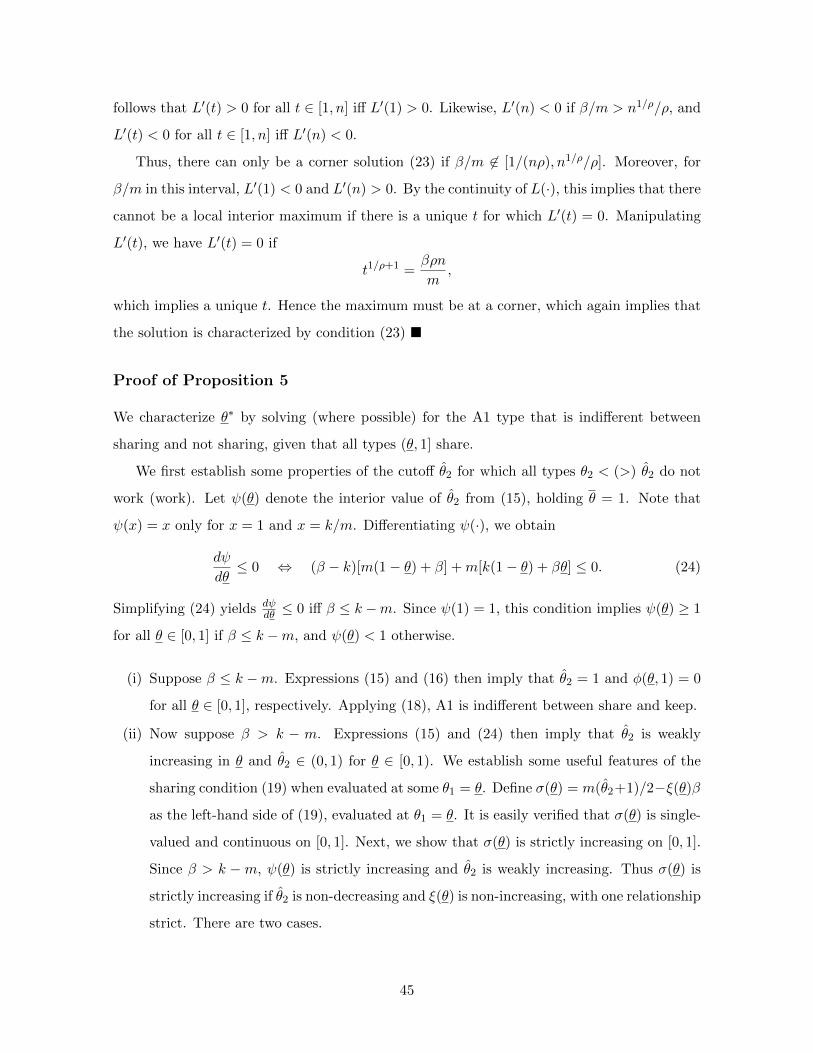
follows that L′(t) > 0 for all t ∈ [1, n] iff L′(1) > 0. Likewise, L′(n) < 0 if β/m > n1/ρ/ρ, and

L′(t) < 0 for all t ∈ [1, n] iff L′(n) < 0.

Thus, there can only be a corner solution (23) if β/m 6∈ [1/(nρ), n1/ρ/ρ]. Moreover, for

β/m in this interval, L′(1) < 0 and L′(n) > 0. By the continuity of L(·), this implies that there

cannot be a local interior maximum if there is a unique t for which L′(t) = 0. Manipulating

L′(t), we have L′(t) = 0 if

t1/ρ+1 =βρn

m,

which implies a unique t. Hence the maximum must be at a corner, which again implies that

the solution is characterized by condition (23) �

Proof of Proposition 5

We characterize θ∗ by solving (where possible) for the A1 type that is indifferent between

sharing and not sharing, given that all types (θ, 1] share.

We first establish some properties of the cutoff θ2 for which all types θ2 < (>) θ2 do not

work (work). Let ψ(θ) denote the interior value of θ2 from (15), holding θ = 1. Note that

ψ(x) = x only for x = 1 and x = k/m. Differentiating ψ(·), we obtain

dψ

dθ≤ 0 ⇔ (β − k)[m(1− θ) + β] +m[k(1− θ) + βθ] ≤ 0. (24)

Simplifying (24) yields dψdθ ≤ 0 iff β ≤ k −m. Since ψ(1) = 1, this condition implies ψ(θ) ≥ 1

for all θ ∈ [0, 1] if β ≤ k −m, and ψ(θ) < 1 otherwise.

(i) Suppose β ≤ k −m. Expressions (15) and (16) then imply that θ2 = 1 and φ(θ, 1) = 0

for all θ ∈ [0, 1], respectively. Applying (18), A1 is indifferent between share and keep.

(ii) Now suppose β > k − m. Expressions (15) and (24) then imply that θ2 is weakly

increasing in θ and θ2 ∈ (0, 1) for θ ∈ [0, 1). We establish some useful features of the

sharing condition (19) when evaluated at some θ1 = θ. Define σ(θ) = m(θ2+1)/2−ξ(θ)β

as the left-hand side of (19), evaluated at θ1 = θ. It is easily verified that σ(θ) is single-

valued and continuous on [0, 1]. Next, we show that σ(θ) is strictly increasing on [0, 1].

Since β > k −m, ψ(θ) is strictly increasing and θ2 is weakly increasing. Thus σ(θ) is

strictly increasing if θ2 is non-decreasing and ξ(θ) is non-increasing, with one relationship

strict. There are two cases.

45

a. Suppose that k/m ≤ 1. Observe that for θ ≤ k/m, θ2 = ψ(θ) ≥ θ, and when

θ > k/m, θ2 = k/m < θ. Thus by (17), when θ ≤ k/m, ξ(θ) = 1 (i.e., A2 always

wins conditional upon working). Since dψdθ > 0, σ(θ) is strictly increasing. When

θ > k/m, ξ(θ) = (1 − θ)/(1 − k/m) is obviously strictly decreasing in θ. Since θ2

is weakly increasing, σ(θ) is again strictly increasing.

b. Suppose that k/m > 1. Now for all θ, θ2 = ψ(θ) ≥ θ; thus by the argument for

k/m ≤ 1 and θ ≤ k/m, ξ(θ) = 1 and σ(θ) is strictly increasing. Since σ(θ) is

increasing, A1 does not share if limθ→1 σ(θ) ≤ 0. There are two subcases. First,

let k/m ≤ 1. Note that θ2 = k/m at θ = 1 and ξ(1) = 0, so substituting into σ(·)

the condition for no sharing becomes:

m

2

(k

m+ 1

)< 0. (25)

This condition is obviously impossible to satisfy, and so σ(1) ≥ 0 and A1 does not

choose keep for all θ1. Second, let k/m > 1. By (15), θ2 = 1 at θ = 1 and ξ(θ) = 1,

so substituting into σ(·) the condition for no sharing simplifies to m < β. Thus A1

keeps for all θ1 when m < min{k, β}.

(iii) Full sharing occurs in equilibrium if and only if σ(0) ≥ 0. Note that ξ(0) = 1, so

substituting into σ(·) the condition for full sharing becomes

m

2

(k

m+ β+ 1

)− β > 0

m

2(k +m)− m

2β − β2 > 0. (26)

It is easily shown that the last expression has only one positive root, and so all types

share if

β <−m+

√m2 + 8m(k +m)

4.

(iv) There are two cases.

a. Suppose that k/m < 1. If sharing for all θ1 is not possible, then the analogous case

in part (ii) implies that there exists some interior θ∗ such that σ(θ) = 0. Since θ∗

depends on θ2 and θ2 is at a corner at θ = k/m, we consider conditions under which

θ∗ will lie on either side of k/m. As σ(θ) is increasing, θ∗ < k/m iff σ(k/m) > 0,

ork +m

2> β. (27)

46

If (27) holds, then since θ∗ < k/m implies θ2 < k/m, θ∗ is characterized by

substituting ψ(θ) and ξ(θ) = 1 into (19):

m

2

[k(1− θ) + βθ

m(1− θ) + β+ 1

]− β = 0. (28)

The solution to (28) is then easily derived:

θ∗ =m(k − β +m)− 2β2

m(k − 3β +m)(29)

If (27) does not hold, then since θ∗ ≥ k/m implies θ2 = k/m, θ∗ is characterized

by substituting θ2 and ξ(θ) = (1− θ)/(1− k/m) into (19):

m

2

(k

m+ 1

)− 1− θ

1− k/mβ = 0. (30)

The solution to (30) is then easily derived:

θ∗ = 1− m(1− (k/m)2)

2β.

b. Suppose that k/m ≥ 1. From part (ii), m < β implies that A1 always keeps, so we

restrict attention to m ≥ β. We have σ(1) ≥ 0 and θ2 = ψ(θ) > θ for all θ ∈ [0, 1).

Thus, θ2 is interior for all values of θ and θ∗ is characterized by the the value of θ

such that σ(θ) = 0, as given by (29).

Observe finally that given θ∗, according to (18) no type higher (resp., lower) than θ∗ can

strictly benefit from keeping (resp., sharing); thus each type of A1 will play the specified

sharing strategy.

Summarizing all of the derivations yields the claimed result �

Proof of Comment 3

We show that the two possible values of θ∗ are increasing in β. Differentiating m(k−β+m)−2β2

m(k−3β+m)

with respect to β yields the following condition:

2(3β2 + k(m− 2β) +m2 − 2βm

)m(k − 3β +m)2

> 0

⇔ (m− β)2 + 2β(β − k) + km > 0. (31)

There are two possible subcases.

47

1. Suppose k < m. Expression (31) is linear in k and holds at k = 0. At k = m, (31)

evaluates to 2(m− β)2 + β2 > 0, which clearly holds. Thus (31) holds for all k < m.

2. If k ≥ m, then it is sufficient to show that 2β(β − k) + km > 0. Observe that this

expression is linear in m, and for m = k, it evaluates to β2 + (β−k)2 > 0, which clearly

holds. As established in the proof of (iv) in Proposition 5, m ≥ β when k ≥ m, and

so the expression evaluates to 2β2 − kβ > 0 at m = β. This is true if k < 2β, which

follows from straightforward manipulation of the fact that β >−m+√m2+8m(k+m)

4 in

any interior equilibrium. Next, differentiating 1 − m(1−(k/m)2)2β with respect to β yields

the following condition:

(1− k2/m2)m

2β2> 0.

Since k/m < 1 for the subcase in which this value of θ∗ applies, this expression clearly

holds �

B Instructions

You are participating in a study on economic decision making and will be asked to make a

number of decisions. For your participation, you will receive a show-up fee of $5. Please read

these instructions carefully as they describe how you can earn additional money.

All the interaction between you and other participants will take place through the com-

puters. Please do not communicate with other participants. If you have a question, raise your

hand and one of us will help you.

The study is anonymous. In other words, your identity will not be revealed to others

and the identity of others will not be revealed to you.

During the study your earnings will be expressed in points. Points will be converted to

dollars at the following rate: 100 points = $10. You will be paid your earnings in cash.

The study is divided into 60 periods. At the end of the study, we will randomly select

one period (each with equal probability). Your earnings today will equal the number of

points you obtained in that randomly-selected period (plus the $5 show-up fee).

The decisions to be made in each period are described below.

48

Decisions in each period

In each period, you will interact with one other participant. Note that you will be randomly

paired with a different participant at the beginning of each period. Moreover, decisions

from past periods will not be revealed.

At the beginning of each period, both participants receive an endowment of 110 points.

In addition, each participant will be randomly assigned to a role and a productivity level.

Specifically, one participant will be randomly assigned to the role of Player A and the other

participant to the role of Player B. The participant in the role of Player A will be randomly

assigned to a Low, Intermediate, or High productivity level (each being equally likely).

The participant in the role of Player B is always assigned to the High productivity level.

Each period is divided into two subsequent stages: a pre-investment stage, which is

then followed by an investment stage.

Pre-investment stage

In this stage, Player A receives an investment opportunity. Player A then decides whether

Player B can take part in the investment opportunity. Specifically, Player A chooses between

the following three options:

• Only A can invest

• Only B can invest

• Both A and B can invest

Investment stage

In this stage, players who can invest decide whether to invest or not invest. If a player does

not invest, he/she does not incur any costs and does not produce income. If a player invests,

he/she incurs a cost of 220 points and produces an amount of income that depends on the

player’s productivity according to Table I below.

The total income produced is divided into two types of income and is distributed among

the two players in the following way:

• Constant income: this type of the income is always distributed equally between Player

A and Player B. Moreover, it is received irrespective of whether players could make an

49

Table I. Total income produced depending on productivity

Productivity of the investing player Total income produced

Low productivity 210 points

Intermediate productivity 285 points

High productivity 360 points

investment decision or not, and if they could, irrespective of whether the players invested

or not.

• Varying income: this type of the income is distributed only among the players that

could make an investment decision. In other words:

– If Player A chose “only A can invest” then Player A receives all the varying income.

– If Player A chose “only B can invest” then Player B receives all the varying income.

– If Player A chose “Both A and B can invest” then both players receive varying

income. The amount each player receives depends on the total amount of income

each player generates. Recall that a player generates income by investing; if he/she

does not invest then he/she generates 0 points. The precise share received by each

player is given by Table II.

Table II. Varying income if Player A chose “both A and B can invest”

Productivity ofTotal income Share of varying

produced by income for

A B A B A B

Low High 210 points 360 points 30% 70%

Low High 210 points 0 points 78% 22%

Low High 0 points 360 points 3% 97%

Intermediate High 285 points 360 points 40% 60%

Intermediate High 285 points 0 points 88% 12%

Intermediate High 0 points 360 points 3% 97%

High High 360 points 360 points 50% 50%

High High 360 points 0 points 97% 3%

High High 0 points 360 points 3% 97%

50

Screenshot of Player A’s pre-investment choice

To familiarize you with the screen in which you will make decisions, look at the provided

screenshot in which Player A makes the pre-investment choice. In this example, 50% of the

total income is allocated to constant income and the remaining 50% is allocated varying

income.

To help with the understanding of the way income and earnings are calculated, we will

walk you through the calculations seen in the screen above. Note that while you are making

decisions these calculations are already made for you. We simply go through them here to

illustrate how they are done.

I. As you can see, irrespective of Player A’s pre-investment choice, if neither Player A nor

Player B invests then both players earn their endowment: 110 points.

II. If only A can invest and he/she does invest then:

• The earnings of Player A equal: A’s endowment (110 points) the cost of investing

(220 points) + A’s constant income (142 × 50% = 71 points) + all the varying

income (143 points) = 104 points.

• The earnings of Player B equal: B’s endowment (110 points) + B’s constant income

51

(142 × 50% = 71 points) = 181 points.

III. If only B can invest and he/she does invest then:

• The earnings of Player A equal: A’s endowment (110 points) + A’s constant income

(180 × 50% = 90 points) = 200 points.

• The earnings of Player B equal: B’s endowment (110 points) the cost of investing

(220 points) + B’s constant income (180 × 50% = 90 points) + all the varying

income (180 points) = 160 points.

• Note that, compared to case II, the constant and varying incomes are larger here

because Player B is the one who invests and Player B has a higher productivity

level than Player A.

IV. If both A and B can invest and both players invest then:

• The earnings of Player A equal: A’s endowment (110 points) the cost of investing

(220 points) + A’s constant income (322 × 50% = 161 points) + A’s share of the

varying income (323 × 40% = 129 points) = 180 points.

• The earnings of Player B equal: B’s endowment (110 points) the cost of investing

(220 points) + B’s constant income (322 × 50% = 161 points) + B’s share of the

varying income (323 × 60% = 194 points) = 245 points.

• Note that when both players invest, the constant and varying incomes are largest

because both players generate income.

V. If both A and B can invest but only Player A invests then:

• The earnings of Player A equal: A’s endowment (110 points) the cost of investing

(220 points) + A’s constant income (142 × 50% = 71 points) + A’s share of the

varying income (143 × 88% = 125 points) = 86 points.

• The earnings of Player B equal: B’s endowment (110 points) + B’s constant income

(142 × 50% = 71 points) + B’s share of the varying income (143 × 12% = 18 points)

= 199 points.

• Note that, as in case II, in this case Player A is the only one generating the constant

and varying incomes. However, unlike in case II, Player A does not receive all the

varying income, which is why Player A’s earnings are lower and Player B’s earnings

are higher (compared to case II).

52

VI. If both A and B can invest but only Player B invests then:

• The earnings of Player A equal: A’s endowment (110 points) + A’s constant income

(180 × 50% = 90 points) + A’s share of the varying income (180 × 3% = 5 points)

= 205 points.

• The earnings of Player B equal: B’s endowment (110 points) the cost of investing

(220 points) + B’s constant income (180 × 50% = 90 points) + B’s share of the

varying income (180 × 97% = 175 points) = 155 points.

The precise division of total income into constant income and varying income will change

during the study. You will be told when such a change occurs.

This concludes the instructions. Please click on the red button on your screen. If you

have any questions then raise your hand and we will be happy to assist.

C Statistical analysis

In this section we describe in detail the statistical analysis supporting the experimental results.

C.1 Regression analysis pooling on the theoretical predictions

Here we provide the regressions used to construct the 95% confidence intervals seen in Fig-

ure 3 in the main body of the paper. In all regressions, the only independent variables are

dummy variables indicating each of the predicted outcomes (collaboration being the omit-

ted outcome). Table C1 reports the marginal effects of the estimated coefficients and their

respective standard errors.15 We cluster standard errors on the 24 matching groups.

Regression I in Table C1 corresponds to A1’s first stage choice. We estimate the coef-

ficients using a multinomial probit regression using A1’s choice to either keep (column Ia),

refer (column Ib), or share (column Ic) jurisdiction as the dependent variable. The next two

regressions correspond to probit regressions where the dependent variable equals one if A1

exerted effort in the second stage. Regression II restricts the sample to periods in which A1

decided to keep jurisdiction and regression III to periods in which A1 decided to share juris-

diction. Similarly, regressions IV and V correspond to probit regressions where the dependent

15Marginal effects are estimated with respect to the case where all independent variables are zero. In other

words, they indicate the mean change in behavior compared to the collaboration outcome.

53

Table C1. Regressing equilibrium outcomes on observed behavior

Ia Ib Ic II III IV V VI

Indifference 0.00 0.12 −0.12 −0.87 −0.74 −0.83 −0.73 −0.70

(0.01) (0.01) (0.02) (0.05) (0.03) (0.05) (0.03) (0.02)

Delegation −0.03 0.34 −0.31 −0.79 −0.95 −0.03 −0.07 −0.43

(0.01) (0.02) (0.02) (0.06) (0.01) (0.03) (0.01) (0.01)

Turf war 0.78 −0.01 −0.77 0.07 −0.01 0.03 0.01 −0.58

(0.03) (0.01) (0.03) (0.03) (0.03) (0.03) (0.01) (0.01)

No. obs. 5760 643 4195 922 4195 5760

Note: Marginal effects and thier respective standard errors in parenthesis.

variable equals one if A2 exerted effort in the second stage. Regression IV restricts the sample

to periods in which A1 decided to refer jurisdiction and regression V to periods in which A1

decided to share jurisdiction. Finally, regression VI is an OLS regression estimating the effect

of the model’s predictions on total welfare as a fraction of the maximum welfare (i.e., the sum

of both players’ payoffs when both have a high productivity, jurisdiction, and exert effort:

W (θ1 + θ2)− 2k = 0.74).16

The regressions from Table C1 can also be used to test whether there are statistically

significant differences in behavior between equilibrium predictions. Since we are making

multiple pairwise Wald tests for each variable, we determine statistical significance based

on Bonferroni-adjusted p-values. Specifically, for the jurisdiction decision, we multiply p-

values by 18 since we run one test per pairwise comparison for each of the three outcomes

(keep, refer, and share). For the effort choices, we multiply p-values by 12 since we run one

test per pairwise comparison for each jurisdiction choice (keep and share for A1, and refer

and share for A2). Lastly, for welfare, we multiply p-values by 6 since we run one test per

pairwise comparison. The results of these pairwise comparisons are presented in Table C2.

The pairwise comparisons from the regressions give very similar results as those from

nonparametric tests (reported in Table 3 in the main body of the paper). There are only two

differences between these results and those from the nonparametric tests. First, A2s effort

after a referral is now significantly higher in a turf war compared to indifference, which is

16Results are vary similar if instead of the probit regressions we use logit regressions with subject fixed effects

and instead of an OLS we use a linear regression with subject fixed effects. The fixed-effects regressions are

available upon request.

54

Table C2. Pairwise comparisons between equilibrium predictions

Agent Action

Treatment comparisons

Indif. Indif. Indif. Deleg. Deleg. Collab.

vs. vs. vs. vs. vs. vs.

Deleg. Collab. Turf Collab. Turf Turf

A1

Keep ∗∗ ∗∗ ∗∗ ∗∗

Refer ∗∗ ∗∗ ∗∗ ∗∗ ∗∗

Share ∗∗ ∗∗ ∗∗ ∗∗ ∗∗ ∗∗

Effort (after keep) ∗∗ ∗∗ ∗∗ ∗∗

Effort (after share) ∗∗ ∗∗ ∗∗ ∗∗ ∗∗

A2Effort (after refer) ∗∗ ∗∗ ∗∗ ∗∗

Effort (after share) ∗∗ ∗∗ ∗∗ ∗∗ ∗∗

Both Welfare ∗∗ ∗∗ ∗∗ ∗∗ ∗∗ ∗∗

Note: Pairwise comparisions between equilibrium predictions based on

the regressions in Table C1. ∗∗ and ∗ indicate statistical significance at

1% and 5% using Bonferroni-adjusted p-values.

consistent with the theoretical predictions. Second, the small difference in A2s effort rate

between delegation and turf war (6 percentage points) appears as statistically significant.

C.2 Statistical analysis of individual treatments

Here we provide the detailed statistical analysis of the subjects behavior in the individual

treatments. Figure 4 in the main body of the paper presents the mean actions taken by A1s

and A2s over all periods for each of the 12 combinations of β and θ1. Going from the top-

left to the bottom-right, the first three graphs show the mean fraction of times A1s choose

to keep, refer, or share jurisdiction. The next four graphs show the mean fraction of times

A1s/A2s exert effort (conditional on having jurisdiction, depending on whether they were

sharing jurisdiction or not. Lastly, the eighth graph shows mean total welfare as a fraction of

the maximum welfare.

To test whether the differences observed in Figure 3 are statistically significant, we ran

both regressions and nonparametric tests. We start with the nonparametric analysis. Once

again, we construct our independent observations by averaging the subjects’ behavior within

each matching group, which gives us 24 observations per treatment (all matching groups

experienced all the parameter combinations). We then performed all pairwise treatment com-

55

parisons using Wilcoxon-signed-rank tests. We use Bonferroni-adjusted p-values to avoid false

positives due to multiple comparisons. Specifically, for the jurisdiction choice, we multiply

p-values by 198 since we run one test for each of the 66 pairwise comparisons for each of the

three jurisdiction choices (i.e., for the keeping rate, the referral rate, and the sharing rate).

For A1’s effort rate, A2’s effort rate, and welfare, we we multiply p-values by 66 since we run

one test per pairwise comparison.17

In Table C3 we present pairwise comparisons between treatments that have the same

productivity for A1. In other words, these tests allow us to observe one if the most interesting

predictions of the model, Namely, the non-monotonic effect of increasing the prize β at the

different productivity levels θ1 ∈ {0.55, 0.75, 0.95}. The other treatment comparisons are not

reproduced here but can be obtained by rerunning our statistical analysis using provided

do-file and dataset (we used the statistics software STATA version 13.1).

We start discussing the effort decision. Consistent with the theoretical predictions, we

observe that increasing the prize clearly increases A2’s likelihood of exerting effort (when β

increases from 0.15 to 0.50) and A1’s likelihood of exerting effort when A1 is of intermediate

productivity (when β increases from 0.50 to 0.80) or high productivity (when β increases from

0.15 to 0.50) but not when A1 is of low productivity. There are a few statistically significant

differences that are not inline with the theoretical predictions. However, they tend to be

small (at most 10 percentage points) and might occur because, as argued by Goeree and Holt

(1999), mistakes are bound to be made more often when they are less costly. In this case, not

exerting effort when one benefits from doing so is less costly for lower βs.

For the jurisdiction decision, we observe that, as predicted, increasing β to 0.95 strongly

increases the likelihood that A1 keeps jurisdiction when A1 is of intermediate productivity

but not when A1 is of low or high productivity. The most obvious deviation from the model’s

prediction is the high propensity of A1 of intermediate productivity to refer jurisdiction instead

of sharing it when β = 0.50. Once again, this can be explained by mistakes being made more

often when they are less costly (e.g., referring instead of sharing implies a loss of 2% of A1s

profits when β = 0.50 but a 9% of A1s profits when β = 0.80).

Lastly, we look at the treatment differences in welfare. In line with the theoretical predic-

tions, when A1 is of intermediate productivity welfare significantly increases as β increases

17In this analysis, we do not separate the effort rate depending on the jurisdiction choice because, if we do,

there are too few independent observations for various treatment comparisons.

56

Table C3. Treatments differences in behavior

Keep Refer ShareA1’s A2’s

Welfareeffort effort

θ55β15 vs. θ55β50 0.07∗ −0.38∗∗ 0.30∗∗ 0.02 −0.73∗∗ −0.73∗∗

θ55β15 vs. θ55β80 0.06 −0.07 0.01 0.08∗ −0.81∗∗ −0.80∗∗

θ55β15 vs. θ55β95 −0.01 0.05 −0.04 0.07∗ −0.81∗∗ −0.73∗∗

θ55β50 vs. θ55β80 −0.01 0.31∗ −0.29∗ 0.06 −0.08∗ −0.07

θ55β50 vs. θ55β95 −0.08 0.43∗∗ −0.34∗∗ 0.05 −0.08 0.00

θ55β80 vs. θ55β95 −0.07 0.12 −0.05 −0.01 0.00 0.07

θ75β15 vs. θ75β50 0.04 −0.33∗∗ 0.29∗ 0.07 −0.69∗∗ −0.45∗∗

θ75β15 vs. θ75β80 −0.03 0.11 −0.08 −0.78∗∗ −0.79∗∗ −0.74∗∗

θ75β15 vs. θ75β95 −0.79∗∗ 0.13∗∗ 0.66∗∗ −0.84∗∗ −0.79∗∗ −0.24∗∗

θ75β50 vs. θ75β80 −0.07 0.44∗∗ −0.37∗∗ −0.85∗∗ −0.10∗ −0.29∗∗

θ75β50 vs. θ75β95 −0.83∗∗ 0.46∗∗ 0.37∗∗ −0.91∗∗ −0.10∗ 0.21∗∗

θ75β80 vs. θ75β95 −0.76∗∗ 0.02 0.74∗∗ −0.06∗ 0.00 0.50∗∗

θ95β15 vs. θ95β50 0.02 0.04 −0.07 −0.53∗∗ −0.59∗∗ −0.56∗∗

θ95β15 vs. θ95β80 −0.02 0.08∗ −0.07∗ −0.53∗∗ −0.63∗∗ −0.58∗∗

θ95β15 vs. θ95β95 −0.05 0.08∗ −0.04 −0.54∗∗ −0.63∗∗ −0.56∗∗

θ95β50 vs. θ95β80 −0.04 0.04 0.00 0.03 −0.04 −0.02

θ95β50 vs. θ95β95 −0.07 0.04 0.03 −0.01 −0.04 0.00

θ95β80 vs. θ95β95 −0.03 0.00 0.03 −0.01 0.00 0.02

Note: Mean differences in observed behavior between treatments. ∗∗ and ∗

indicate statistical significance at 1% and 5% according to Wilcoxon signed-

ranks tests using matching-group means and Bonferroni-adjusted p-values.

from 0.15 to 0.50 and then to 0.80, but then significantly decreases as β reaches 0.95. By

contrast, when A1 is of low or high productivity, welfare significantly increases as β increases

from 0.15 to 0.50 but then does not decrease with further increases in β.

We also analysed the data using regressions. In all regressions, the independent variables

correspond to dummy variables indicating each of the treatments (the omitted treatment is

θ55β15). We ran the same type of regressions as those reported in Table C1. Namely, regression

I is a multinomial probit regression using A1’s choice to either keep (column Ia), refer (column

Ib), or share (column Ic) jurisdiction as the dependent variable. Regressions II and III are

probit regressions where the dependent variable is A1’s (regression II) or A2’s (regression III)

effort choice conditional on having jurisdiction. Lastly, regression IV is an OLS regression

57

Table C4. Regressing treatments on observed behavior

Ia Ib Ic II III IV

θ55β50 −0.07 0.38 −0.31 −0.02 0.73 0.37

(0.03) (0.18) (0.15) (0.03) (0.03) (0.02)

θ55β80 −0.06 0.07 −0.01 −0.08 0.81 0.40

(0.03) (0.05) (0.05) (0.02) (0.02) (0.01)

θ55β95 0.01 −0.05 0.04 −0.07 0.80 0.37

(0.03) (0.04) (0.03) (0.02) (0.02) (0.02)

θ75β15 −0.03 −0.04 0.07 0.06 0.05 0.06

(0.02) (0.02) (0.02) (0.02) (0.03) (0.01)

θ75β50 −0.07 0.29 −0.22 0.00 0.73 0.38

(0.03) (0.15) (0.12) (0.03) (0.03) (0.01)

θ75β80 0.00 −0.15 0.15 0.85 0.83 0.60

(0.02) (0.05) (0.05) (0.02) (0.02) (0.01)

θ75β95 0.76 −0.17 −0.59 0.90 0.84 0.24

(0.03) (0.11) (0.11) (0.02) (0.02) (0.01)

θ95β15 −0.03 −0.10 0.13 0.36 0.21 0.32

(0.02) (0.02) (0.02) (0.04) (0.03) (0.03)

θ95β50 −0.06 −0.14 0.20 0.89 0.80 0.87

(0.02) (0.06) (0.04) (0.02) (0.03) (0.02)

θ95β80 −0.02 −0.18 0.20 0.90 0.84 0.89

(0.03) (0.14) (0.12) (0.02) (0.02) (0.01)

θ95β95 0.01 −0.18 0.17 0.90 0.84 0.88

(0.02) (0.11) (0.10) (0.02) (0.02) (0.01)

No. obs. 5760 4838 5117 5760

Note: Marginal effects and thier respective standard er-

rors in parenthesis.

with total welfare as a fraction of the maximum welfare as the dependent variable. Table C4

reports the marginal effects of the estimated coefficients and their respective standard errors.18

Standard errors are clustered on the 24 matching groups.19

Using the regressions reported in Table C4, we use Wald tests to evaluate whether there are

statistically significant differences between treatments. To determine statistical significance,

18As before, marginal effects are estimated for the case where all independent variables are zero.

19The results are very similar if we use logit regressions with subject fixed effects for the effort choices and

a linear regression with subject fixed effects for total welfare. These regressions are available upon request.

58

Table C5. Pairwise comparisons between treatments

Keep Refer ShareA1’s A2’s

Welfareeffort effort

θ55β15 vs. θ55β50∗∗ ∗∗

θ55β15 vs. θ55β80∗ ∗∗ ∗∗

θ55β15 vs. θ55β95∗ ∗∗ ∗∗

θ55β50 vs. θ55β80∗∗

θ55β50 vs. θ55β95∗

θ55β80 vs. θ55β95

θ75β15 vs. θ75β50∗∗ ∗∗

θ75β15 vs. θ75β80∗∗ ∗∗ ∗∗

θ75β15 vs. θ75β95∗∗ ∗∗ ∗∗ ∗∗ ∗∗

θ75β50 vs. θ75β80∗∗ ∗ ∗∗

θ75β50 vs. θ75β95∗∗ ∗∗ ∗∗ ∗∗

θ75β80 vs. θ75β95∗∗ ∗∗ ∗∗ ∗∗

θ95β15 vs. θ95β50∗∗ ∗∗ ∗∗

θ95β15 vs. θ95β80∗∗ ∗∗ ∗∗

θ95β15 vs. θ95β95∗∗ ∗∗ ∗∗

θ95β50 vs. θ95β80∗∗

θ95β50 vs. θ95β95∗∗

θ95β80 vs. θ95β95

Note: Pairwise comparisions between treatments based on

the regressions in Table C4. ∗∗ and ∗ indicate statistical sig-

nificance at 1% and 5% using Bonferroni-adjusted p-values.

we adjust p-values using the same method as in the nonparametric analysis. Table C5 presents

the significance of the same pairwise comparisons presented in Table C3.

By and large, pairwise comparisons based on the regressions give very similar results as

those based on nonparametric tests (see Table C3). On one hand, a few of the small treatment

differences in A1’s and A2’s effort decision are now statistically significant at the 5% level.

On the other hand, in the jurisdiction decision, the differences in the referral rate that are

statistically significant with the nonparametric tests are not significant with the regressions.

However, both statistical approaches arrive to the same conclusion: A1’s of intermediate

productivity (but not A1’s of low or high productivity) keep jurisdiction more when the prize

is high, which produces an inverse U-shape relationship between prize size and welfare.

59