Reliability of Structures

Professor Assoc. Professor

Benjamin W. Schafer

Discussion over the design assumption of buckling

length “ 2a” for studs braced by sheathing

Student: Luiz Vieira May/2008

1. Introduction Since AISI (1962) to the newest version of AISI-COFS (2007) stud buckling

should be checked in the weak-axis over a length of two times the fastener spacing, a.

Figure 1 shows the configuration assumed. The idea behind the assumption is that would

be safe in the case that the fastener is missed or ineffective consider that the column

buckles over a length 2a. The arbitrary number 2a has been carried over the codes for 46

years without any reliability study found.

The project makes an effort to understand the model and provide an overview of

the problem, providing information to be considered in further studies.

a) Buckling over length “a” b) Buckling over length “2a” Figure 1 – Buckling length.

2. Statistics study of the tests for spring stiffness The literature review about spring stiffness conducted to the research developed

by Fiorino et al. (2006), the tests are illustrated on Figure 2. Basically, the idea for the

test is pull or push two C sections connected to a strip and study the stiffness provided for

the connections between C section and the strip. The material used for the strips were

gypsum and plywood. For this project only the data for plywood was used.

a) Specimen and test machine b) Device Figure 2 – Test conception (Fiorino et al. (2006)).

Different kinds of failure modes were found, Figure 3, and coupling of the modes

illustrated were reported too. The test varied the strand orientation, the load direction,

load rate and the loaded edge distance. From a reliability study point of view, too many

variables were admitted for the number of test, but knowing the lack of study in this area

the results encountered provide reasonable data to base this project.

a) Tilting of screw b) Pull-through sheathing c) Tilting o f screw and bearing in the sheathing

d) Breaking of sheathing edge

Figure 3 – Failure modes (Fiorino et al. (2006)).

To a reliability study the data has to be approximated by a good fitting curve. In

the case studied Figure 4a shows the comparison between lognormal and normal CDF

curve generation. It is clear that the lognormal curve provide better results than the

normal curve. Figure 4b shows the results acquired generating lognormal distributed

random numbers using the Matlab’s function.

0 0.5 1 1.5 2 2.50

0.1

0.2

0.3

0.4

0.5

0.6

0.7

0.8

0.9

1

x

Cum

ulat

ive

frequ

ency

or F

x(x)

Lognormal CDF

Lognormal fitNormal fit

0 0.5 1 1.5 2 2.5 30

0.1

0.2

0.3

0.4

0.5

0.6

0.7

0.8

0.9

1

x

Cum

ulat

ive

frequ

ency

or F

x(x)

Lognormal CDF for 100 values generated

a) Comparison between lognormal and normal fitting b) Results using lognormal random generation of data Figure 4 – Function fitting and data generated.

In fact, lognormal distribution is the best fitting but it can’t be assumed to be an

excellent solution. Figure 5 shows the relative frequency histogram and the PDF fitting,

as can be seen, it is a rough approximation. Definitely, it would be worth conduct more

test decreasing the number of variables and increasing the number of tests. For this

project was assumed a lognormal distribution based on the data available.

0.4 0.6 0.8 1 1.2 1.4 1.6 1.8 2 2.2 2.40

0.5

1

1.5

2

2.5

3

3.5

4

x

Rel

ativ

e Fr

eque

ncy

or p

x(x)

Relative Frequency Histogram and PDF FIT

Figure 5 – Relative frequency histogram and PDF fitting.

3. Example studied The example chosen is slightly different as the one presented in the design manual

AISI – COFS (2001), Figure 6. Cross-section, material properties and fastener spacing

were assumed deterministic variables. The spring stiffness associated to the lateral

restriction provided by the wall is the variable studied, as soon as, the probability of

failure for the same.

Figure 6 – Example studied (Design Manual – COFS (2001))

Two results have to be highlighted: a) Buckling over the length 2a as proposed by

the code is Pcr=pi^2*E*I/(2a)^2=pi^2*29500*0.1133/(2*8)^2=128.86kips and b)

Buckling over length a is Pcr=515.43kips. Those numbers are reference for further

discussions.

The examples analyzed differentiate from the example in the design manual,

because the total length of the column is considered 100in. In this case are admitted 2in

between the wall edge and the first and last fastener, then the 96in. between the first and

last fastener is multiple of 16in (2a) and 8in (a).

4. Model to analyze beam on discrete spring In order to develop a solution for the problem of a beam on multiples discrete

springs the energy method was assumed. Due to the difficulty to find a closed solution for

the problem Rayleigh-Ritz method was used.

Rayleigh-Ritz method is based on assume a displacement function that satisfy the

boundary conditions, then the total potential energy function reduces from a functional to

a function and can be used ordinary calculus to solve the problem, Chen and Lui (1987).

The deflection shape is represented in equation 1.

∑ ∑= =

==n

i

n

iiii L

xiaa1 1

)sin( πφν (1)

The strain energy, equation 2, can be simplified to equation 3, and the

differentiation in relation to a1, a2, …, an is represented for equation 4.

∫=L

dxdx

vdEIU0

22

2

)(21

(2)

∑=

=n

i

i

LiaEIU

13

424

4π

(3)

3

44

2LnaEI

aU n

n

π=

∂∂

(4)

The potential energy due to the force P, equation 5 can be simplified to equation

6, and the differentiation is represented in equation 7.

∫−

=L

P dxdxvdPV

0

2)(2

(5)

∑=

−=n

i

iP L

iaPV1

222

4π

(6)

LnaP

aV n

n

P

2

22π−=

∂∂

(7)

The variables na

U∂∂ and

n

P

aV

∂∂ will turn to be a matrix that fills only the main

diagonal due to the independence of the crossed terms, but in the case of the potential

energy due to the springs the crossed terms has to be considered. The potential energy

due to the springs is represented in the equation 8, the differentiation follows a rule which

is presented in equation 9. In equation 9, n represents the line in the matrix and j the

column that will form the matrix. The final matrix will always be of dimension n x n.

∑ ∑ ⎟⎠

⎞⎜⎝

⎛=

=

ns n

iis L

xiakV1

2

1)sin(

21 π

(8)

)sin()sin(),(

1 Lxj

Lxnk

ajnV ns

n

S ππ⋅=

∂∂ ∑

(9)

The sum of the equations 4, 7 and 9 by energy equilibrium is equal to zero, then it

is formed the eigenvalue problem.

A Matlab routine was developed to analyze the problem and vary the spring

stiffness based on the lognormal distribution. The program is in the appendix 10.2. The

program also permits the variation of the probability of failure for each spring using a

linear function.

5. Comparison with ABAQUS model

To confirm the results using the Matlab program one of the examples was

simulated in ABAQUS, the input is in the Appendix 10.1. The example was defined in

chapter 3. Figure 7 shows a sketch of the problem as soon as the restrictions adopted to

force the column to buckle in the direction that the springs are effective and the

eigenvector for the first mode.

a) Model to be studied b) FEM and rigid restrictions

c) Springs position d) Eigenvector for the first mode (eigenvalue=146.23kips)

Figure 7 – ABAQUS model.

The eigenvector for the first mode is not composed for the same number of half-

waves than the spaces between springs, what means that the springs does not provide

enough restriction to the column to buckle between connections. By another way, the

lengths of half-waves are not equal to 2a, although the number is very close for this

example.

The eigenvalue identified using ABAQUS was 146.23kips and using the Matlab

program the value is 148.11kips. The small difference between FEM and the energy

method (Rayleigh-Ritz) can be explained by the fact that both assumptions are

approximated solutions for the problem. Hence, the Matlab routine was considered a

good approximation.

Another comment is how close the results are to the value calculated in chapter 3,

(Pcr(@2a)=128.86kips), and has to be said that the difference of 13% is acceptable

considering the lack of a reliability knowledge to analyze the problem. The results are

close because of the fact that the half-wave length formed for this spring stiffness is close

to 2a, if it was not true the difference can be bigger. Remember that the spring stiffness

are based on the material plywood but it could be gypsum which present low values for

the spring stiffness and consequently the number of waves would be less and the

assumption 2a would be unsafe. The consideration of a buckling length of 2a is

reasonable but can be better.

6. Model studied

Two considerations can be done to analyze the problem: a) associate a probability

of failure to each point connected in the column, Figure 1, or b) associate a probability of

failure to each fastener that connects to the stud, Figure 8. The difference will be if

happens a failure in a, the point in the column is complete ineffective, by another way

considering b the point in the column can still have the contribution of the another spring.

In fact, what happens is case b, where the probability of failure of each spring is

uncorrelated, but case a is the case that the codes are based.

Figure 8 – Explanation of each point connected.

6.1 Probability of failure in each point connected, case a

Figure 9 shows the study done for case a, the probability of failure vary from 0 to

10%, for each probability of failure were analyzed 1000 models. All the values are

plotted for the fastener spacing of 8in. (circles), as soon as the mean and the bounds

(mean plus and minus standard deviation), in order to compare are plotted the results for

fastener spacing of 16in. and probability of failure 0%.

The comparison between fastener spacing of 8 and 16in. shows that it is very

conservative consider the distance 16in. based on the assumption that the fastener can be

missed or over-drifted. As was expected the mean decrease and the standard deviation

increase with the probability of failure, more discussion about the results are in the next

section.

0 2 4 6 8 100

10

20

30

40

50

60

70

80

90

Probability of failure (%)

Pcr

Probability associated to each spot (double spring)

mean

mean + std

mean - std

fast. spac.=16in.

mean + std

mean - std

Figure 9 – Variation of Pcr for different probability of failure.

6.2. Probability of failure associate to each spring, case b

As the same way were done the simulations for the case b. Figure 10 shows the

results, comparing the results to the previous simulations definitely case b conduct to

results more uniform and with smaller values for standard deviation.

0 2 4 6 8 100

10

20

30

40

50

60

70

80

90

Probability of failure (%)

Pcr

Probability associated to each spring

mean

fast. spac.=16in.

mean + std

mean - std

Figure 10 - Variation of Pcr for different probability of failure.

For a design engineer point of view what really matters is the partial safety factor,

φ, assuming that the coefficient of variation and mean of the professional factor are equal

to 1, φ can be defined as equation 10.

PVpe μφ β55.0−= (10)

Assuming the reliability index, β, equal 3.5, Table 1 presents the φ values found.

Table 1 – Values of φ for cases a and b.

Pf=0% Pf=1% Pf=2% Pf=5% Pf=8% Pf=10% Case a 0.34 0.30 0.27 0.20 0.16 0.13 Case b 0.36 0.35 0.34 0.31 0.28 0.27

Consider case a or b makes difference when calculate the partial safety factor, and

in a real system case b is what really happens. The partial safety factor apparently assume

values very small, what contributes to this is the fact that the relation between the mean

critical load and the critical load assuming mean values for the spring stiffness is very

small.

7. Conclusions

As soon as, the engineers are able to model the column on discrete springs, how

was explained in this project, the partial safety factors are defined in Table 1. Considering

the buckling over the length 2a is definitely too conservative, if it is a tentative to

compute the probability to the fastener be over-drifted or missed.

By another way, seems that consider buckling over 2a is a tentative to adapt the

Euler column to the column on discrete spring. Anyway, doesn’t make sense hide this

valuable information knowing the innumerous tools that are available nowadays.

8. Future research

The problem of lateral buckling on a column can be extended to a more

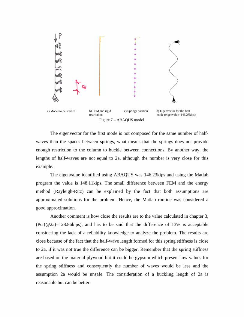
complicated system where is considered the actual section. The simulation, Figure 11,

lead to local and distortional buckling what is certainly a huge field to be explored.

Figure 11 – The real problem configuration.

9. References American Iron and Steel Institute (1962). Light Gage Cold-Formed Steel Design Manual. New York, NY. American Iron and Steel Institute (2007). North American Standard for Cold-formed Steel Framing-Wall Stud Design. Washington, D.C. ABAQUS. (2007). “ABAQUS/Standard Version 6.7-1.”, Dassault Systèmes, http://www.simulia,com/, Providence, RI. Chen, W.F., Lui, E. M., (1987). “Structural Stability”, Elsevier, New York, NY. Nowak, A. S., Collins, R.C., (2000). “Reliability of Structures”, McGRAW-HILL International Editions. Fiorino, L., Della Corte, G., Landolfo, R., (2006). ‘Experimental tests on typicall screw connections for cold-formed steel housing.” Engineering Structures. Elsevier Science. Vol.29, No,8, pp. 1761-1773. 10. Appendix 10.1 Abaqus inp file *HEADING *PREPRINT, MODEL=YES FLEXURAL BUCKLING *RESTART,WRITE,FREQUENCY=999 *NODE 1,0.0,0.0,0.0 101,100,0.0,0.0 *NGEN,NSET=ALL 1,101 *ELEMENT,TYPE=B31OS 1,1,2 *ELGEN,ELSET=BEAM

1,100,1,1 *BEAM GENERAL SECTION,SECTION=GENERAL,ELSET=BEAM 0.327,0.1133,0,0.1133,100 0.0, 0.0, -1.0 29500 *Element, type=spring1 101,3 102,11 103,19 104,27 105,35 106,43 107,51 108,59 109,67 110,75 111,83 112,91 113,99 *Elset, elset=spring1, generate 101,113,1 *Spring, elset=spring1 2,2 13.0868 *BOUNDARY 101,1,3 1,2,3 ALL,3 *STEP *BUCKLE 5, *CLOAD 1,1,1. *END STEP

10.2 Matlab program close all clear all clc %Generate k OSB %Test data osb_k=[1.30 1.42 1.22 1.73 1.07 1.27 0.85 1.13 1.07 1.10 0.82 0.77 1.11 0.92 1.39 2.05 1.05 1.10 1.11 1.82 1.28 0.92 0.77 0.98 0.73 0.86 1.10]; %Trasformation of units kN/mm to kip/in (google='1kN/mm in pound/in'divide by 1000) osb_k=osb_k/0.175126835; mean_osb_k=mean(osb_k); std_osb_k=std(osb_k); %Change for lognormal sigma_ln_osb_k=(log((std_osb_k/mean_osb_k)^2+1))^0.5; mean_ln_osb_k=log(mean_osb_k)-0.5*(std_osb_k)^2; %Datas lt=100;

x=[2:8:98]; E=29500; I=0.1133; n=length(x); pf=10 %probability of failure in % %Loop to change number of simulation for sim=1:1000 %Spring's Matrix generation - Us for i=1:n for j=1:n % Random generation of ks1 ks1=lognrnd(mean_ln_osb_k,sigma_ln_osb_k,1,1); if ks1<0 ks1=0; else end % Active or not act=rand(1,1); act=act>pf/100; ks1=ks1*act; % Random generation of ks2 ks2=lognrnd(mean_ln_osb_k,sigma_ln_osb_k,1,1); if ks2<0 ks2=0; else end % Active or not act=rand(1,1); act=act>pf/100; ks2=ks2*act; %Final spring stiffness ks=ks1+ks2; plus=0; for k=1:length(x) Us(i,j)=plus+ks*sin(i*pi*x(k)/lt)*sin(j*pi*x(k)/lt); plus=Us(i,j); end end end %Strain Energy's Matrix - Ub for m=1:n Ub(m,m)=(E*I*(pi)^4*(m)^4)/(2*(lt)^3); end %Potential Energy's Matrix without contribution of spring for m2=1:n V(m2,m2)=((pi^2*m2^2)/(2*lt)); end %Build Matrix not dependent of P

U=Ub+Us; %Find eigenvalue P(:,sim)=eig(U,V); minimum(sim)=min(P(:,sim)); end %Find statistic of the minimum P found in each simulation Pmean=mean(minimum) Pstd=std(minimum) exp1=exp(-0.55*3.5*std(minimum)/mean(minimum)) %Save variable for more studies save('Pcr_8_pf10_2xk', 'minimum')