Lecture  2    

Discrete  Production  Plants    

Introduction  A  discrete  production  process  is  the  assembly  of  pieces  and  parts  into  products  and  the  product   result   as   a   discrete   entity.     Discrete   processes   deal  with  material   that   can   be  counted.   The   equipment  used   in   the  process   do  not  work   in   a   steady   state  mode,   but  rather  in  a  startup  –  operate  –  shut  down  mode.    An   example   of   a   discrete   production   process   is   the   automotive   industry,   e.g.   the  production  of  cars,  see  Figure  1.  The  production  line  starts  with  the  truck  coming  in  with  raw  material  such  as  metallic  sheets.  The  first  work  cell  performs  Stamping.  A  stamping  die  is  a  specialized  tool  used  to  cut  or  shape  materials  using  a  press.  The  second  work  cell  is  the  Body  in  white,  in  which  the  remaining  activities  in  the  production  of  a  vehicle  body  are  performed.  After  Body   in  White,   the  Paintwork   takes  place;   here   the  vehicle  body   is   painted   in   the   correct   color.   The   next   to   last   work   cell   is   the   Body   assembly  where   the   interior   of   the   car   is   installed,   e.g.,   dashboard,   gear,   seats   and   doors.   After  inspection,  the  cars  are  loaded  on  a  truck  for  shipment  to  the  retailer  or  customer.      

     

Figure  1:  A  schema  of  a  discrete  production  plant.    

There  are  a  number  of  characteristics  typical  to  discrete  processes:  • The  product  is  a  discrete  entity.    • Assembly-­‐oriented  production.  • Staged  production  through  work  cells  • Well-­‐defined  production  runs.  • The  process  is  most  often  “visible”.  • The  equipment  operates  in  on-­‐off  manner.  • The  production  process  is  sequential.    

 

Control  of  Discrete  Production  Plants  Discrete  manufacturing   is   typically   assembly-­‐line   oriented.   It   involves   the  progressive  assembly  of   finished  products  via  a  number  of  work  cells,  each  providing  a  predefined  set  of  mechanical  operations.  The  equipment  performing   these  operations  operates   in  on-­‐off   manner.   In   order   to   structure   the   on-­‐off   of   the   machines   sequential   control  languages  are  used.    The  basic  device  invented  for  control  of  discrete  production  processes  is  the  automatic  switch  and  interconnected  sequences  of  automatic  switches.  The  first  automatic  switch  to   be   extensively   used   for   control   of   discrete   production   processes   was   the  electromechanical   relay,   see   Figure   2.   The   electromechanical   relays   were   typically  assembled  on  relay  panels   in  a  manner  that  would  accomplish  the  desired  automation  steps,  referred  to  as  “relay  ladders”.      

   

Figure  2:  Electromechanical  relay    

Formal  specification  languages  and  formal  modeling  techniques  are  used  to  describe  the  behaviour  of  the  equipment  and/or  production  process.  Formal  analysis  techniques  are  then   used   to   verify   certain   critical   properties.   A   number   of   approaches   have   been  developed.  They  are  based  on;  logics,  finite  state  machines,  and  Petri  Nets.      There  are  different  tools  and  languages  for  implementation  of  discrete  controllers.  With  better  abstraction  and  structuring  possibilities  it  is  easier  to  get  a  good  overview  of  the  control   problem   and   the   implementation   is   drastically   simplified.   Most   of   these   tools  and   languages  are  graphical  programming   languages.  Grafcet   is  one  example  of  such  a  language.  Grafcet  is  now  part  of  the  IEC  1131-­‐3  standard  (later  renamed  IEC  61131-­‐3),  under   the   name   Sequential   Function   Charts   (SFC).   JGrafchart   is   a   toolbox   based   on  Grafcet,   implemented   in   Java.   JGrafchart   was   developed   at   Department   of   Automatic  Control,  LTH,  Lund  University.        

Logic  The  concept  used  in  the  construction  of  relay  ladders  is  boolean  logic.  In  boolean  logic,  the  variables  are  either  true  or  false.  Boolean  logic  is  named  after  George  Boole  (1815-­‐1864),  who  first  defined  an  algebraic  system  of   logic   in  the  mid-­‐19th  century.  Boolean  logic  is  based  on  three  operations;  and,  or,  not.                          The  operations  can  be  represented  by  graphical  symbols.  Figure  3  shows  the  symbols,  the  American  representation  to  the  right  and  the  Swedish  representation  to  the  left.    

 Figure  3:  Boolean  logic  symbols  

Three  types  of  operations  

     

AND   𝑎 ∙ 𝑏   a  and  b   a∧ b  

OR   a  +  b   a  or  b   a∨ b  

NOT   𝑎  (𝑜𝑟  𝑎!)   not  a   !a  

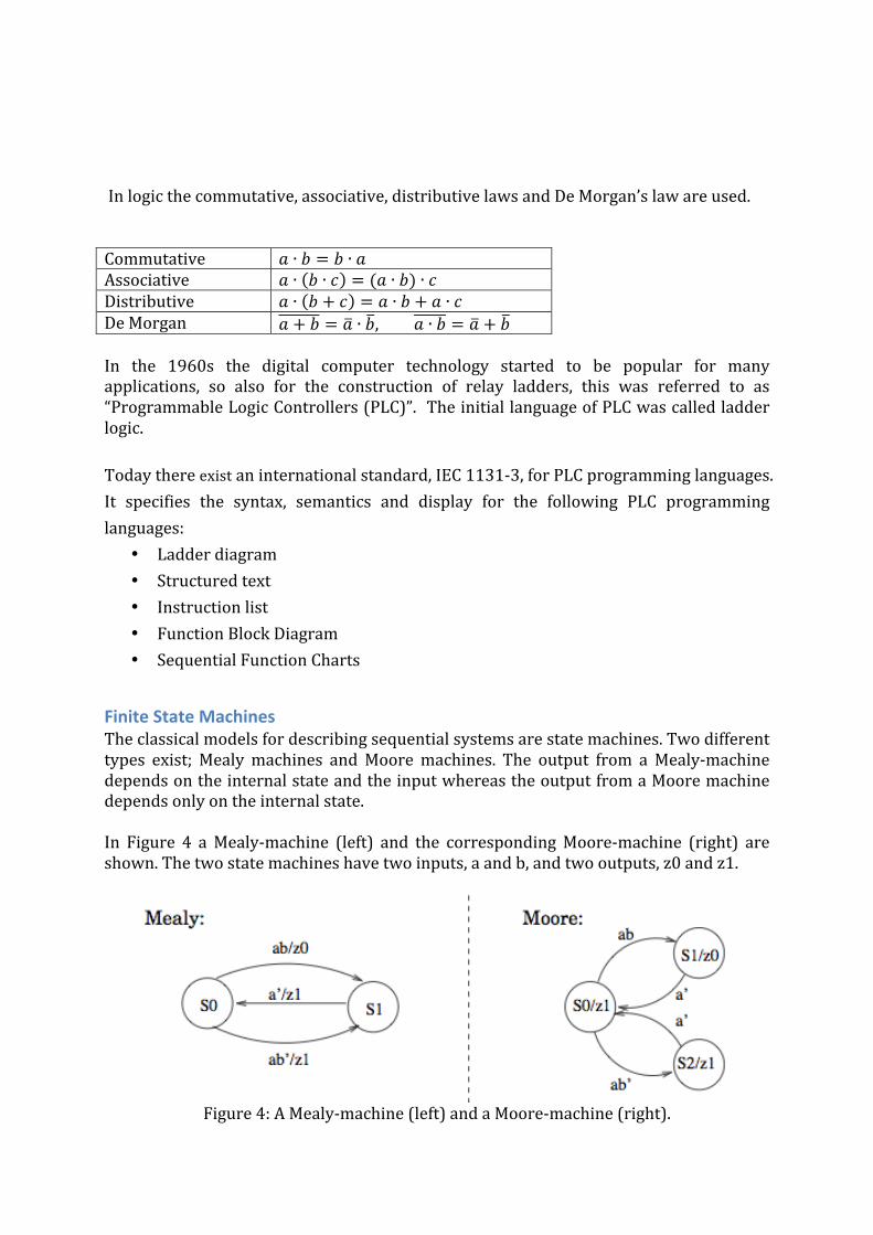
         In  logic  the  commutative,  associative,  distributive  laws  and  De  Morgan’s  law  are  used.            Commutative   𝑎 ∙ 𝑏 = 𝑏 ∙ 𝑎  Associative   𝑎 ∙ 𝑏 ∙ 𝑐 = (𝑎 ∙ 𝑏) ∙ 𝑐  Distributive   𝑎 ∙ 𝑏 + 𝑐 = 𝑎 ∙ 𝑏 + 𝑎 ∙ 𝑐  De  Morgan   𝑎 + 𝑏 = 𝑎 ∙ 𝑏, 𝑎 ∙ 𝑏 = 𝑎 + 𝑏    In   the   1960s   the   digital   computer   technology   started   to   be   popular   for   many  applications,   so   also   for   the   construction   of   relay   ladders,   this   was   referred   to   as  “Programmable  Logic  Controllers  (PLC)”.    The  initial  language  of  PLC  was  called  ladder  logic.      Today  there  exist  an  international  standard,  IEC  1131-­‐3,  for  PLC  programming  languages.  It   specifies   the   syntax,   semantics   and   display   for   the   following   PLC   programming  languages:  

• Ladder  diagram  • Structured  text  • Instruction  list  • Function  Block  Diagram  • Sequential  Function  Charts  

 

Finite  State  Machines  The  classical  models  for  describing  sequential  systems  are  state  machines.  Two  different  types   exist;   Mealy  machines   and  Moore  machines.   The   output   from   a  Mealy-­‐machine  depends  on  the  internal  state  and  the  input  whereas  the  output  from  a  Moore  machine  depends  only  on  the  internal  state.    In   Figure   4   a  Mealy-­‐machine   (left)   and   the   corresponding  Moore-­‐machine   (right)   are  shown.  The  two  state  machines  have  two  inputs,  a  and  b,  and  two  outputs,  z0  and  z1.    

 Figure  4:  A  Mealy-­‐machine  (left)  and  a  Moore-­‐machine  (right).  

 A  common  application  in  today’s  vehicles  is  the  cruise  control.  The  cruise  control  system  has   a   human-­‐machine   interface   that   allows   it   to   communicate   with   driver   to  communicate   with   the   system.   There   are   many   ways   to   implement   this   system;   one  version   is   illustrated  by   the   finite   state  machine   in  Figure  5.  When   the  driver   sets   the  speed  of   the  vehicle,   the   vehicle   goes   into   the  Cruise   state.  When   the  vehicle   is   in   the  Cruise  state,  the  driver  can  go  back  to  manual  driving  by  giving  the  command  cancel.  If  the  driver  hits  the  breaks  while  being  in  the  Cruise  state,  the  vehicle  reduces  the  speed.    When  the  driver  let  go  of  the  break  the  car  goes  back  to  the  Cruise  state  and  the  previous  set  speed.  The  driver  also  has  the  option  of  completely  switching  the  Cruise  controller  off.      

                               Figure  5:  The  state  machine  of  a  cruise  controller  (left)  and  the  operator  commands  in  

the  vehicle.  

Petri  Nets  Petri   nets   were   proposed   by   the   German   mathematician   Carl   Adam   Petri   in   the  beginning   of   the   1960s.   Petri   wanted   to   define   a   general   purpose   graphical   and  mathematical   model   describing   relations   between   conditions   and   events.   The  mathematical  modeling  ability  of  Petri  nets  makes  it  possible  to  set  up  state  equations,  algebraic   equations,   and  other  models   governing   the  behavior  of   the  modeled   system.  The  graphical  feature  makes  Petri  nets  suitable  for  visualization  and  simulation.    The   Petri   net  model   has   two  main   interesting   characteristics.   Firstly,   it   is   possible   to  visualize  behavior  like  parallelism,  concurrency,  synchronization  and  resource  sharing.  Secondly,  there  exists  a  large  number  of  theoretical  methods  for  analysis  of  these  nets.  Petri   nets   can   be   used   at   all   stages   of   system   development:   modeling,   mathematical  analysis,   specification,   simulation,   visualization,   and   realization.   Petri   nets   have   been  used   in   a   wide   range   of   application   areas,   e.g.,   performance   evaluation,   distributed  database   systems,   flexible   manufacturing   systems,   logic   controller   design,  multiprocessor  memory  systems,  and  asynchronous  circuits.      Petri   nets   have   during   the   years   been   developed   and   extended   and   several   special  classes   of   Petri   nets   have   been   defined.   These   include,   e.g.:   generalized   Petri   nets,  synchronized  Petri   nets,   timed  Petri   nets,   interpreted  Petri   nets,   stochastic   Petri   nets,  continuous  Petri  nets,  hybrid  Petri  nets,  coloured  Petri  nets,  object-­‐oriented  Petri  nets,  and  multidimensional  Petri  nets.    

A  Petri  net  (PN)  has  two  types  of  nodes:  places  and  transitions  see  Figure  6.  A  place  is  represented   as   a   circle   and   a   transition   is   represented   as   a   bar   or   a   small   rectangle.  Places   and   transitions  are   connected  by  arcs.  An  arc   is  directed  and   connects   either   a  place  with  a  transition  or  a  transition  with  a  place,  i.e.,  a  PN  is  a  directed  bipartite  graph.  A  transition  without  an  input  place  is  called  a  source  transition  and  a  transition  without  an  output  place  is  called  a  sink  transition.      

   

Figure  6:  Petri  Net    Systems  with  concurrency  can  be  modeled  with  Petri  nets  using  the  and-­‐divergence  and  the  and-­‐convergence  structure,  see  Figure  7  (left).  Systems  with  conflicts  or  choices  can  be   modeled   using   the   or-­‐divergence   and   the   or-­‐convergence   structure,   see   Figure   7  (right).    

 Figure  7:  Concurrency  and  Conflict  

 A   transition   is   enabled   if   each   of   its   input   places   contains   at   least   one   token.   An  autonomous  PN   is  a  PN  where   the   firing   instants  are  either  unknown  or  not   indicated  whereas  a  non-­‐autonomous  PN  is  a  PN  where  the  firing  of  a  transition  is  conditioned  by  external  events  and/or  time.  

 An  enabled  transition  in  an  autonomous  PN  may  or  may  not  fire.  An  enabled  transition  in   a  non-­‐autonomous  PN   is   said   to  be   fireable  when   the   transition   condition  becomes  true.   A   fireable   transition  must   fire   immediately.   The   firing   of   a   transition   consists   of  removing  one  token  from  each  input  place  and  adding  one  token  to  each  output  place  of  the  transition.  The  firing  of  a  transition  has  zero  duration.    Petri  Nets  can  be  analyzed  with  respect  to  several  properties:  

• Live:  No  transitions  can  become  unfireable  • Deadlock-­‐free:  Transitions  can  always  be  fired  • Bounded:  Finite  number  of  tokens  

 The  analysis  methods  are:  

• Reachability  methods  –  exhaustive  enumeration  of  all  possible  markings  • Linear  algebra  methods  –  describe  the  dynamic  behaviour  as  matrix  equations  • Reduction  methods–   transformation   rules   that   reduce   the   net   to   a   simpler   net  

while  preserving  the  properties  of  interest    Other  types  of  Petri  Nets  are  

• Generalized  Petri  Nets:  Weights  associated  to  the  arcs  • Times  Petri  Nets:  Times  associated  with  transitions  or  places  • High-­‐Level  Petri  Nets:  Tokens  are  structured  data  types  (objects)  • Continuous   &   Hybrid   Petri   Nets:   The   markings   are   real   numbers   instead   of  

integers.  Mixed  continuous/discrete  systems    Petri   nets   can   conveniently   be   used   to   model   systems   with   e.g.,   concurrency,  synchronization,   parallelism   and   resource   sharing.   The   graphical   nature   of   Petri   nets  also  makes  them  suitable  to  use  for  visualization  and  simulation  of  systems.  In  addition  to  this,  the  nets  can  be  theoretically  analyzed  with  different  analysis  methods.    

Grafcet  Grafcet  was  proposed  in  France  in  1977  as  a  formal  specification  and  realization  method  for   logical   controllers.  The  name  Grafcet  was  derived   from  “graph”,   since   the  model   is  graphical   in   nature,   and   “AFCET”   (Association   Francaise   pour   la   Cybernetique  Economique  et  Technique),  the  scientific  association  that  supported  the  work.    During   several   years,   Grafcet  was   tested   in   French   industries.   It   soon   proved   to   be   a  convenient   tool   for   representing   small   and  medium   scale   sequential   systems.   Grafcet  was   therefore   introduced   in   the   French   educational   programs   and   proposed   as   a  standard   to   the   French   association   AFNOR   where   it   was   accepted   in   1982.   In   1988  Grafcet,   with   minor   changes,   was   also   adopted   by   the   International   Electro-­‐technical  Commission  (IEC)  as  an  international  standard  named  IEC  848.  In  this  standard  Grafcet  goes   under   the  name   Sequential   Function  Chart   (SFC).   Seven   years   later,   in   1995,   the  standard   IEC   1131-­‐3,   with   SFC   as   an   essential   part,   arrived.   The   standard   concerns  programming  languages  used  in  Programmable  Logic  Controllers  (PLC).   It  defines  four  different  programming   language  paradigms  together  with  SFC.  No  matter  which  of   the  four  different  languages  that  is  used,  a  PLC  program  can  be  structured  with  SFC.    

Because  of  the  two  international  standards,  Grafcet,  or  SFC,  is  today  widely  accepted  in  industry,  where  it  is  used  as  a  representation  format  for  sequential  control  logic  at  the  local  PLC  level.    Grafcet  has  a  graphical  syntax.  It  is  built  up  by  steps,  drawn  as  squares,  and  transitions,  represented  as  bars.  The  initial  step,  i.e.,  the  step  that  should  be  active  when  the  system  is   started,   is   represented   as   a   double   square.   Grafcet   has   support   for   both   alternative  and  parallel  branches,  see  Figure  8.    

   

Figure  8:  Grafcet  graphical  syntax.    A  step  can  be  active  or  inactive.  An  active  step  is  marked  with  one  (and  only  one)  token  placed  in  the  step.  The  steps  that  are  active  define  the  situation  or  the  state  of  the  system.  To  each  step  one  or  several  actions  can  be  associated.  The  actions  are  performed  when  the  step  is  active.    Transitions  are  used  to  connect  steps.  Each  transition  has  a  receptivity.  A   transition   is  enabled   if   all   steps   preceding   the   transition   are   active.   When   the   receptivity   of   an  enabled  transition  becomes  true  the  transition  is  fireable.  A  fireable  transition  will  fire  immediately.  When  a  transition  fires  the  steps  preceding  the  transition  are  deactivated  and   the   steps   succeeding   the   transition   are   activated,   i.e.,   the   tokens   in   the   preceding  steps  are  deleted  and  new  tokens  are  added  to  the  succeeding  steps.    

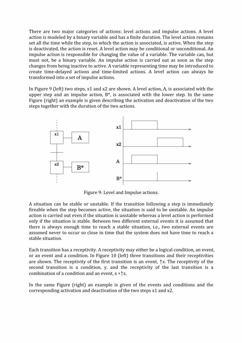
There   are   two  major   categories   of   actions:   level   actions   and   impulse   actions.   A   level  action  is  modeled  by  a  binary  variable  and  has  a  finite  duration.  The  level  action  remains  set  all  the  time  while  the  step,  to  which  the  action  is  associated,  is  active.  When  the  step  is  deactivated,  the  action  is  reset.  A  level  action  may  be  conditional  or  unconditional.  An  impulse  action  is  responsible  for  changing  the  value  of  a  variable.  The  variable  can,  but  must   not,   be   a   binary   variable.   An   impulse   action   is   carried   out   as   soon   as   the   step  changes  from  being  inactive  to  active.  A  variable  representing  time  may  be  introduced  to  create   time-­‐delayed   actions   and   time-­‐limited   actions.   A   level   action   can   always   be  transformed  into  a  set  of  impulse  actions.      In  Figure  9  (left)  two  steps,  x1  and  x2  are  shown.  A  level  action,  A,  is  associated  with  the  upper   step   and   an   impulse   action,   B*,   is   associated  with   the   lower   step.   In   the   same  Figure  (right)  an  example  is  given  describing  the  activation  and  deactivation  of  the  two  steps  together  with  the  duration  of  the  two  actions.      

 Figure  9:  Level  and  Impulse  actions.  

 A   situation   can  be   stable  or  unstable.   If   the   transition   following   a   step   is   immediately  fireable  when  the  step  becomes  active,   the  situation   is  said  to  be  unstable.  An   impulse  action  is  carried  out  even  if  the  situation  is  unstable  whereas  a  level  action  is  performed  only   if   the  situation   is  stable.  Between  two  different  external  events   it   is  assumed  that  there   is   always   enough   time   to   reach   a   stable   situation,   i.e.,   two   external   events   are  assumed  never  to  occur  so  close  in  time  that  the  system  does  not  have  time  to  reach  a  stable  situation.    Each  transition  has  a  receptivity.  A  receptivity  may  either  be  a  logical  condition,  an  event,  or  an  event  and  a  condition.  In  Figure  10  (left)  three  transitions  and  their  receptivities  are  shown.  The  receptivity  of   the   first   transition   is  an  event,  ↑x.  The  receptivity  of   the  second   transition   is   a   condition,   y,   and   the   receptivity   of   the   last   transition   is   a  combination  of  a  condition  and  an  event,  x  ∗↑z.    In   the   same   Figure   (right)   an   example   is   given   of   the   events   and   conditions   and   the  corresponding  activation  and  deactivation  of  the  two  steps  x1  and  x2.    

 Figure  10:  Three  transitions  and  their  receptivities  

 To   facilitate   the  description  of   large  and  complex   systems  macro  steps   can  be  used.  A  macro   step   is   a   step   with   an   internal   representation   that   facilitates   the   graphical  representation  and  makes  it  possible  to  detail  certain  parts  separately.  A  macro  step  has  one  input  and  one  output  step.  When  the  transition  preceding  the  macro  step  fires  the  input  step  of  the  macro  step  is  activated.  The  transition  succeeding  the  macro  step  does  not  become  enabled  until   the  execution  of   the  macro  step  reaches   its  output  step.  The  macro  step  concept  is  shown  in  Figure  11.    

   

Figure  11:  A  macro  step.    The  dynamic  behavior  of  Grafcet  is  defined  by  five  rules:  

1. The  initial  situation  of  a  Grafcet  is  determined  by  its  initial  steps.    2. A  transition  is  enabled  if  all  of  its  previous  steps  are  active.  A  enabled  transition  

is  fireable  if  its  associated  receptivity  is  true.  A  fireable  transition  is  immediately  fired.  

3. Firing  of  a  transition  results  in  deactivation  of  its  previous  step  and  a  simultaneous  activation  of  its  following  steps.  

4. Simultaneously  fireable  transitions  are  simultaneously  fired.  5. If  an  active  step  is  to  be  simultaneously  deactivated  and  activated  it  remains  

active.    The   aim   of   Grafcet,   or   SFC,   in   the   standards   has   gradually   shifted   from   being   a  representation   format   for   logical   controllers   towards   being   a   graphical   programming  language   for   sequential   control   problems   at   the   local   level.   One   main   advantage   of  Grafcet,  or  SFC,  is  its  simple  and  intuitive  graphical  syntax.  Today  Grafcet  is  widely  used  and  well  accepted  in  industry.    

JGrafchart  JGrafchart   is   a   Grafcet/SFC   editor   and   execution   environment   developed   at   the  Department  of  Automatic  Control,  Lund  University.    JGrafchart   provides   graphical   representation   and   execution   of   operation   sequences,  procedures,  and  state  machines.  It  integrates  features  from  Grafcet  in  IEC  61131-­‐3,  and  Statecharts  with  concepts  from  procedural  and  object-­‐oriented  programming.  JGrafchart  is   implemented   in   Java/Swing   and   runs   on   all   platforms   that   support   Java.   The   tool  combines  an  interactive  graphical  programming  environment  with  a  run-­‐time  engine  for  execution  of  JGrafchart  function  charts.  JGrafchart  can  be  used  for  all  types  of  discrete-­‐event  based  applications,  e.g.,  logical  control,  operating  procedure  management,  recipe-­‐based  batch  control,  and  workflow  modelling.  The  high  generality  of  JGrafchart  makes  it  applicable  in  a  wide  variety  of  process  control  and  operator  support  situations.    JGrafchart  supports  the  following  language  elements:    

• workspace  objects  • Steps  • initial  steps  • transitions  • parallel  splits  and  parallel  joins  • macro  steps  • exception  transitions  

In  addition  there  is  support  for:    • digital  inputs  and  digital  outputs  • analog  inputs  and  analog  outputs  • socket  inputs  and  socket  outputs  • internal  variables  (real,  boolean,  string,  and  integer)  • action  buttons  and  free  text  for  comments.  

 Sequence   diagrams   are   created   interactively   using   drag-­‐and-­‐drop   from   a   palette  containing   the   different   language   elements.   The   sequence   diagrams   are   stored   on  JGrafchart  workspace  objects,  see  Figure  12.    

   

Figure  12:  An  example  of  a  JGrafchart.    JGrafchart  is  presented  in  Laboratory  Exercise  1.    

Summary  In  today’s  lecture  the  focus  has  been  on  Discrete  Production  Processes,  see  Figure  13.    

   

Figure  13:  The  discrete  production  process.  

 

References:  • P.  Martin  and  G.Hale  [2010]:  Automation  made  easy.  Published  by  ISA.  ISBN  978-­‐

1-­‐936007-­‐06-­‐6    • C.  Johnsson  [1999]:  A  graphical  language  for  batch  control,  Ph.D  thesis,  Dept.  of  

Automatic  control,  Lund  University,  Number  1051  • R.  David  and  H.  Alla  and  [1992]:  Grafcet  &  Petri  nets:  Tools  for  Modelling  Discrete  

Event  Systems,  Prentice-­‐Hall,  SBN:013327537X  • KJ  Åström  and  R.  Murray  [2008]:  Feedback  Systems:  An  introduction  for  

Scientists  and  Engineers  ,  Princeton  University  Press,  ISBN  978-­‐0-­‐691-­‐13576-­‐2