Embed Size (px)
Citation preview
IEOR E4707: Foundations of Financial Engineering c© 2016 by Martin Haugh
Martingale Pricing Theory in Discrete-Time andDiscrete-Space Models
These notes develop the theory of martingale pricing in a discrete-time, discrete-space framework. This theory isalso important for the modern theory of portfolio optimization as the problems of pricing and portfoliooptimization are now recognized as being intimately related. We choose to work in a discrete-time anddiscrete-space environment as this will allow us to quickly develop results using a minimal amount ofmathematics: we will use only the basics of linear programming duality and martingale theory. Despite thisrestriction, the results we obtain hold more generally for continuous-time and continuous-space models oncevarious technical conditions are satisfied. This is not too surprising as one can imagine approximating theselatter models using our discrete-time, discrete-space models by simply keeping the time horizon fixed and lettingthe number of periods and states go to infinity in an appropriate manner.
1 Martingale Pricing Theory for Single-Period Models
1.1 Notation and Definitions
We first consider a one-period model and introduce the necessary definitions and concepts in this context. Wewill then extend these definitions to multi-period models.
t = 0 t = 1
c����������
c ω1
����������
c ω2
QQQQQQQQQQc ωm
cPPPP
PPPPc
Let t = 0 and t = 1 denote the beginning and end, respectively, of the period. At t = 0 we assume that there
are N + 1 securities available for trading, and at t = 1 one of m possible states will have occurred. Let S(i)0
denote the time t = 0 value of the ith security for 0 ≤ i ≤ N , and let S(i)1 (ωj) denote its payoff at date t = 1 in
the event that ωj occurs. Let P = (p1, . . . , pm) be the true probability distribution describing the likelihood ofeach state occurring. We assume that pk > 0 for each k.
Arbitrage
A type A arbitrage is an investment that produces immediate positive reward at t = 0 and has no future costat t = 1. An example of a type A arbitrage would be somebody walking up to you on the street, giving you a
Martingale Pricing Theory in Discrete-Time and Discrete-Space Models 2
positive amount of cash, and asking for nothing in return, either then or in the future.
A type B arbitrage is an investment that has a non-positive cost at t = 0 but has a positive probability ofyielding a positive payoff at t = 1 and zero probability of producing a negative payoff then. An example of a typeB arbitrage would be a stock that costs nothing, but that will possibly generate dividend income in the future.
In finance we always assume that arbitrage opportunities do not exist1 since if they did, market forces wouldquickly act to dispel them.
Linear Pricing
Definition 1 Let S(1)0 and S
(2)0 be the date t = 0 prices of two securities whose payoffs at date t = 1 are d1
and d2, respectively2. We say that linear pricing holds if for all α1 and α2, α1S(1)0 + α2S
(2)0 is the value of
the security that pays α1d1 + α2d2 at date t = 1.
It is easy to see that absence of type A arbitrage implies that linear pricing holds. As we always assume thatarbitrage opportunities do not exist, we also assume that linear pricing always holds.
Elementary Securities, Attainability and State Prices
Definition 2 An elementary security is a security that has date t = 1 payoff of the formej = (0, . . . , 0, 1, 0, . . . , 0), where the payoff of 1 occurs in state j.
As there are m possible states at t = 1, there are m elementary securities.
Definition 3 A security or contingent claim, X, is said to be attainable if there exists a trading strategy,θ = [θ0 θ1 . . . θN ]>, such that X(ω1)
...X(ωm)
=
S(0)1 (ω1) . . . S
(N)1 (ω1)
......
...
S(0)1 (ωm) . . . S
(N)1 (ωm)
θ0
...θN
. (1)
In shorthand we write X = S1θ where S1 is the m× (N + 1) matrix of date 1 security payoffs. Note that θjrepresents the number of units of the jth security purchased at date 0. We call θ the replicating portfolio.
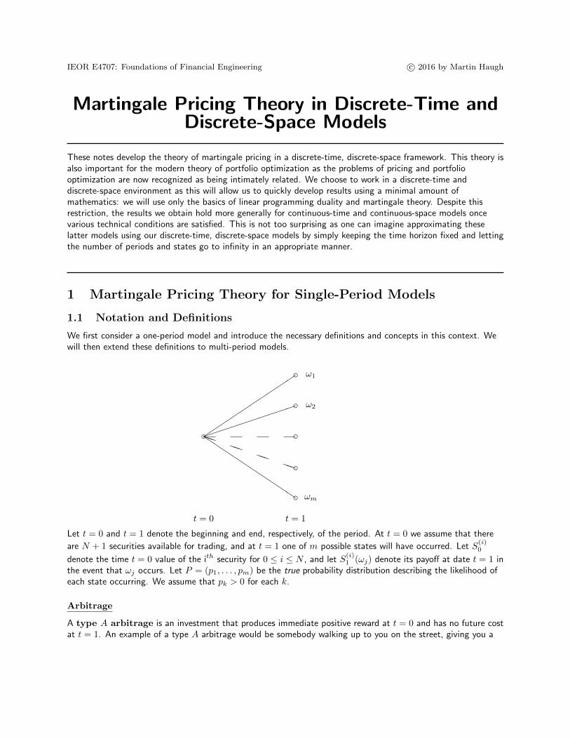
Example 1 (An Attainable Claim)Consider the one-period model below where there are 4 possible states of nature and 3 securities, i.e. m = 4 andN = 2. At t = 1 and state ω3, for example, the values of the 3 securities are 1.03 , 2 and 4, respectively.
t = 0 t = 1
(((((((
((c[1.0194, 3.4045, 2.4917]
hhhhhhhhhHH
HHHHHHH
����
�����
c ω1 [1.03, 3, 2]c ω2 [1.03, 4, 1]
c ω3 [1.03, 2, 4]
c ω4 [1.03, 5, 2]
The claim X = [7.47 6.97 9.97 10.47]> is an attainable claim since X = S1θ where θ = [−1 1.5 2]> is areplicating portfolio for X.
1This is often stated as assuming that “there is no free lunch”.2d1 and d2 are therefore m× 1 vectors.
Martingale Pricing Theory in Discrete-Time and Discrete-Space Models 3
Note that the date t = 0 cost of the three securities has nothing to do with whether or not a claim is attainable.We can now give a more formal definition of arbitrage in our one-period models.
Definition 4 A type A arbitrage is a trading strategy, θ, such that S>0 θ < 0 and S1θ = 0. A type Barbitrage is a trading strategy, θ, such that S>0 θ ≤ 0, S1θ ≥ 0 and S1θ 6= 0.
Note for example, that if S>0 θ < 0 then θ has negative cost and therefore produces an immediate positivereward if purchased at t = 0.
Definition 5 We say that a vector π = [π1 . . . πm]> > 0 is a vector of state prices if the date t = 0 price,P , of any attainable security, X, satisfies
P =
m∑k=1
πkX(ωk). (2)
We call πk the kth state3 price.
Remark 1 It is important to note that in principle there might be many state price vectors. If the kth
elementary security is attainable, then its price must be πk and the kth component of all possible state pricevectors must therefore coincide. Otherwise an arbitrage opportunity would exist.
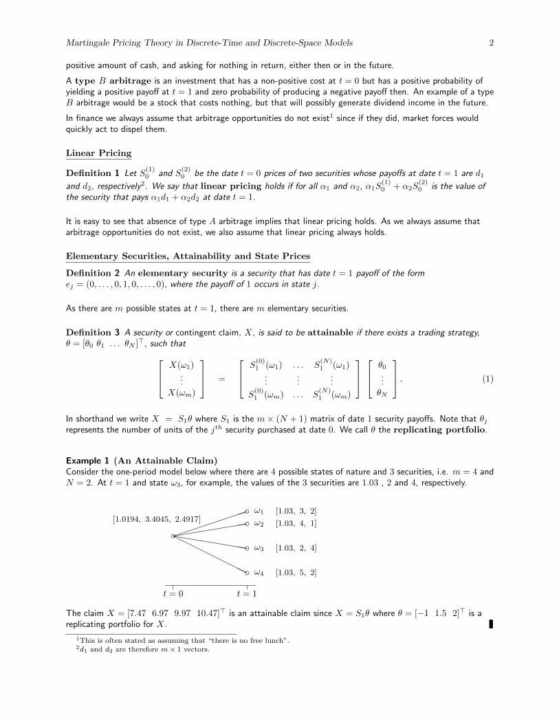
Example 2 (State Prices)Returning to the model of Example 1 we can easily check4 that[π1 π2 π3 π4]> = [0.2433 0.1156 0.3140 0.3168]> is a vector of state prices. More generally, however, we cancheck that
π1π2π3π4
=
0
0.31020.41130.2682
+ ε
0.7372−0.5898−0.29490.1474
is also a vector of state prices for any ε such πi > 0 for 1 ≤ i ≤ 4.
Deflating by the Numeraire Security
Let us recall that there are N + 1 securities and that S(i)1 (ωj) denotes the date t = 1 price of the ith security in
state ωj . The date t = 0 price of the ith security is denoted by S(i)0 .
Definition 6 A numeraire security is a security with a strictly positive price at all times, t.
It is often convenient to express the price of a security in units of a chosen numeraire. For example, if the nth
security is the numeraire security, then we define
S(i)
t (ωj) :=S(i)t (ωj)
S(n)t (ωj)
to be the date t, state ωj price (in units of the numeraire security) of the ith security. We say that we aredeflating by the nth or numeraire security. Note that the deflated price of the numeraire security is alwaysconstant and equal to 1.
3We insist that each πj is strictly positive as later we will want to prove that the existence of state prices is equivalent tothe absence of arbitrage.
4See Appendix A for a brief description of how to find such a vector of state prices.
Martingale Pricing Theory in Discrete-Time and Discrete-Space Models 4
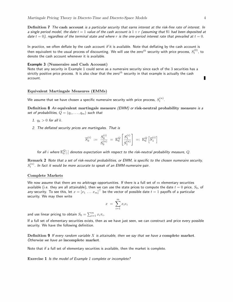
Definition 7 The cash account is a particular security that earns interest at the risk-free rate of interest. Ina single period model, the date t = 1 value of the cash account is 1 + r (assuming that $1 had been deposited atdate t = 0), regardless of the terminal state and where r is the one-period interest rate that prevailed at t = 0.
In practice, we often deflate by the cash account if it is available. Note that deflating by the cash account is
then equivalent to the usual process of discounting. We will use the zeroth security with price process, S(0)t , to
denote the cash account whenever it is available.
Example 3 (Numeraire and Cash Account)Note that any security in Example 1 could serve as a numeraire security since each of the 3 securities has astrictly positive price process. It is also clear that the zeroth security in that example is actually the cashaccount.
Equivalent Martingale Measures (EMMs)
We assume that we have chosen a specific numeraire security with price process, S(n)t .
Definition 8 An equivalent martingale measure (EMM) or risk-neutral probability measure is aset of probabilities, Q = (q1, . . . , qm) such that
1. qk > 0 for all k.
2. The deflated security prices are martingales. That is
S(i)
0 :=S(i)0
S(n)0
= EQ0
[S(i)1
S(n)1
]=: EQ0
[S(i)
1
]for all i where EQ0 [.] denotes expectation with respect to the risk-neutral probability measure, Q.
Remark 2 Note that a set of risk-neutral probabilities, or EMM, is specific to the chosen numeraire security,
S(n)t . In fact it would be more accurate to speak of an EMM-numeraire pair.
Complete Markets
We now assume that there are no arbitrage opportunities. If there is a full set of m elementary securitiesavailable (i.e. they are all attainable), then we can use the state prices to compute the date t = 0 price, S0, ofany security. To see this, let x = [x1 . . . xm]> be the vector of possible date t = 1 payoffs of a particularsecurity. We may then write
x =
m∑i=1
xiei
and use linear pricing to obtain S0 =∑mi=1 xiπi.
If a full set of elementary securities exists, then as we have just seen, we can construct and price every possiblesecurity. We have the following definition.
Definition 9 If every random variable X is attainable, then we say that we have a complete market.Otherwise we have an incomplete market.
Note that if a full set of elementary securities is available, then the market is complete.
Exercise 1 Is the model of Example 1 complete or incomplete?
Martingale Pricing Theory in Discrete-Time and Discrete-Space Models 5
1.2 Pricing in Single-Period Models
We are now ready to derive the main results of martingale pricing theory for single period models.
Proposition 1 If an equivalent martingale measure, Q, exists, then there can be no arbitrage opportunities.
Exercise 2 Prove Proposition 1.
Exercise 3 Convince yourself that if we did not insist on each qk being strictly positive in Definition 8 thenProposition 1 would not hold.
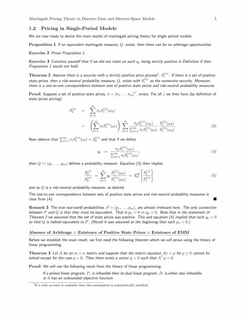
Theorem 2 Assume there is a security with a strictly positive price process5, S(n)t . If there is a set of positive
state prices, then a risk-neutral probability measure, Q, exists with S(n)t as the numeraire security. Moreover,
there is a one-to-one correspondence between sets of positive state prices and risk-neutral probability measures.
Proof: Suppose a set of positive state prices, π = [π1 . . . πm]>, exists. For all j we then have (by definition ofstate prices pricing)
S(j)0 =
m∑k=1
πkS(j)1 (ωk)
=
(m∑l=1
πlS(n)1 (ωl)
)m∑k=1
πkS(n)1 (ωk)∑m
l=1 πlS(n)1 (ωl)
S(j)1 (ωk)
S(n)1 (ωk)
. (3)
Now observe that∑ml=1 πlS
(n)1 (ωl) = S
(n)0 and that if we define
qk :=πkS
(n)1 (ωk)∑m
l=1 πlS(n)1 (ωl)
, (4)
then Q := (q1, . . . , qm) defines a probability measure. Equation (3) then implies
S(j)0
S(n)0
=
m∑k=1
qkS(j)1 (ωk)
S(n)1 (ωk)
= EQ0
[S(j)1
S(n)1
](5)
and so Q is a risk-neutral probability measure, as desired.
The one-to-one correspondence between sets of positive state prices and risk-neutral probability measures isclear from (4).
Remark 3 The true real-world probabilities, P = (p1, . . . , pm), are almost irrelevant here. The only connectionbetween P and Q is that they must be equivalent. That is pk > 0⇔ qk > 0. Note that in the statement ofTheorem 2 we assumed that the set of state prices was positive. This and equation (4) implied that each qk > 0so that Q is indeed equivalent to P . (Recall it was assumed at the beginning that each pk > 0.)
Absence of Arbitrage ≡ Existence of Positive State Prices ≡ Existence of EMM
Before we establish the main result, we first need the following theorem which we will prove using the theory oflinear programming.
Theorem 3 Let A be an m× n matrix and suppose that the matrix equation Ax = p for p ≥ 0 cannot besolved except for the case p = 0. Then there exists a vector y > 0 such that A>y = 0.
Proof: We will use the following result from the theory of linear programming:
If a primal linear program, P , is infeasible then its dual linear program, D, is either also infeasible,or it has an unbounded objective function.
5If a cash account is available then this assumption is automatically satisfied.

Martingale Pricing Theory in Discrete-Time and Discrete-Space Models 6
Now consider the following sequence of linear programs, Pi, for i = 1, . . .m:
min 0>x (Pi)
subject to Ax ≥ εi
where εi has a 1 in the ith position and 0 everywhere else. The dual, Di, of each primal problem, Pi is
max yi (Di)
subject to A>y = 0
y ≥ 0
By assumption, each of the primal problems, Pi, is infeasible. It is also clear that each of the dual problems arefeasible (take y equal to the zero vector). By the LP result above, it is therefore the case that each Di has anunbounded objective function. This implies, in particular, that corresponding to each Di, there exists a vectoryi ≥ 0 with A>yi = 0 and yii > 0, i.e. the ith component of yi is strictly positive. Now taking
y∗ =
m∑i=1
yi,
we clearly see that A>y∗ = 0 and y∗ is strictly positive.
We now prove the following important result regarding absence of arbitrage and existence of positive stateprices.
Theorem 4 In the one-period model there is no arbitrage if and only if there exists a set of positive state prices.
Proof: (i) Suppose first that there is a set of positive state prices, π := (π1, . . . , πm). If x ≥ 0 is the datet = 1 payoff of an attainable security, then the price, S, of the security is given by
S =
m∑j=1
πjxj ≥ 0.
If some xj > 0 then S > 0, and if x = 0 then S = 0. Therefore6 there is no arbitrage opportunity.
(ii) Suppose now that there is no arbitrage. Consider the (m+ 1)× (N + 1) matrix, A, defined by
A =
S(0)1 (ω1) . . . S
(N)1 (ω1)
......
...
S(0)1 (ωm) . . . S
(N)1 (ωm)
−S(0)0 . . . −S(N)
0
and observe (convince yourself) that the absence of arbitrage opportunities implies the non-existence of anN -vector, x, with
Ax ≥ 0 and Ax 6= 0.
In this context, the ith component of x represents the number of units of the ith security that was purchased orsold at t = 0. Theorem 3 then assures us of the existence of a strictly positive vector π that satisfies A>π = 0.We can normalize π so that πm+1 = 1 and we then obtain
S(i)0 =
m∑j=1
πjS(i)1 (ωj).
6This result is really the same as Proposition 1 in light of the equivalence of positive state prices and risk-neutral probabilitiesthat was shown in Theorem 2.
Martingale Pricing Theory in Discrete-Time and Discrete-Space Models 7
That is, π := (π1, . . . , πm) is a vector of positive state prices.
Theorems 2 and 4 imply the following theorem which encapsulates the principal results for our single-periodmodel.
Theorem 5 (First Fundamental Theorem of Asset Pricing)Assume there exists a security with strictly positive price process. Then the absence of arbitrage, the existenceof state prices and the existence of an EMM, Q, are all equivalent.
Example 4 (An Arbitrage-Free Market)The model in Example 1 is arbitrage-free since we saw in Example 2 that a vector of positive state prices existsfor this market
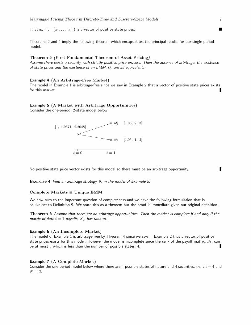
Example 5 (A Market with Arbitrage Opportunities)Consider the one-period, 2-state model below.
t = 0 t = 1
c[1, 1.9571, 2.2048]
hhhhhhhhh
����
�����
c ω1 [1.05, 2, 3]
c ω2 [1.05, 1, 2]
No positive state price vector exists for this model so there must be an arbitrage opportunity.
Exercise 4 Find an arbitrage strategy, θ, in the model of Example 5.
Complete Markets ≡ Unique EMM
We now turn to the important question of completeness and we have the following formulation that isequivalent to Definition 9. We state this as a theorem but the proof is immediate given our original definition.
Theorem 6 Assume that there are no arbitrage opportunities. Then the market is complete if and only if thematrix of date t = 1 payoffs, S1, has rank m.
Example 6 (An Incomplete Market)The model of Example 1 is arbitrage-free by Theorem 4 since we saw in Example 2 that a vector of positivestate prices exists for this model. However the model is incomplete since the rank of the payoff matrix, S1, canbe at most 3 which is less than the number of possible states, 4.
Example 7 (A Complete Market)Consider the one-period model below where there are 4 possible states of nature and 4 securities, i.e. m = 4 andN = 3.
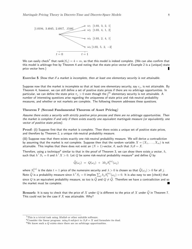
Martingale Pricing Theory in Discrete-Time and Discrete-Space Models 8
t = 0 t = 1
(((((((
((c[1.0194, 3.4045, 2.4917, .1548]
hhhhhhhhhHHH
HHHHHH
����
�����
c ω1 [1.03, 3, 2, 1]c ω2 [1.03, 4, 1, 2]
c ω3 [1.03, 2, 4, 1]
c ω4 [1.03, 5, 2, −2]
We can easily check7 that rank(S1) = 4 = m, so that this model is indeed complete. (We can also confirm thatthis model is arbitrage free by Theorem 4 and noting that the state price vector of Example 2 is a (unique) stateprice vector here.)
Exercise 5 Show that if a market is incomplete, then at least one elementary security is not attainable.
Suppose now that the market is incomplete so that at least one elementary security, say ej , is not attainable. ByTheorem 4, however, we can still define a set of positive state prices if there are no arbitrage opportunities. Inparticular, we can define the state price πj > 0 even though the jth elementary security is not attainable. Anumber of interesting questions arise regarding the uniqueness of state price and risk-neutral probabilitymeasures, and whether or not markets are complete. The following theorem addresses these questions.
Theorem 7 (Second Fundamental Theorem of Asset Pricing)
Assume there exists a security with strictly positive price process and there are no arbitrage opportunities. Thenthe market is complete if and only if there exists exactly one equivalent martingale measure (or equivalently, onevector of positive state prices).
Proof: (i) Suppose first that the market is complete. Then there exists a unique set of positive state prices,and therefore by Theorem 2, a unique risk-neutral probability measure.
(ii) Suppose now that there exists exactly one risk-neutral probability measure. We will derive a contradictionby assuming that the market is not complete. Suppose then that the random variable X = (X1, . . . , Xm) is notattainable. This implies that there does not exist an (N + 1)-vector, θ, such that S1θ = X.
Therefore, using a technique8 similar to that in the proof of Theorem 3, we can show there exists a vector, h,such that h>S1 = 0 and h>X > 0. Let Q be some risk-neutral probability measure9 and define Q̂ by
Q̂(ωj) = Q(ωj) + λhjS(n)1 (ωj)
where S(n)1 is the date t = 1 price of the numeraire security and λ > 0 is chosen so that Q̂(ωj) > 0 for all j.
Note Q̂ is a probability measure since h>S1 = 0 implies∑j hjS
(n)1 (ωj) = 0. It is also easy to see (check) that
since Q is an equivalent probability measure, so too is Q̂ and Q 6= Q̂. Therefore we have a contradiction and sothe market must be complete.
Remark: It is easy to check that the price of X under Q is different to the price of X under Q̂ in Theorem 7.This could not be the case if X was attainable. Why?
7This is a trivial task using Matlab or other suitable software.8Consider the linear program: minθ 0 subject to S1θ = X and formulate its dual.9We know such a Q exists since there are no arbitrage opportunities.
Martingale Pricing Theory in Discrete-Time and Discrete-Space Models 9
2 Martingale Pricing Theory for Multi-Period Models
2.1 Notation and Definitions
Before extending our single-period results to multi-period models, we first need to extend some of oursingle-period definitions and introduce the concept of trading strategies and self-financing trading strategies. Wewill assume10 for now that none of the securities in our multi-period models pay dividends. (We will return tothe case where they do pay dividends at the end of these notes.)
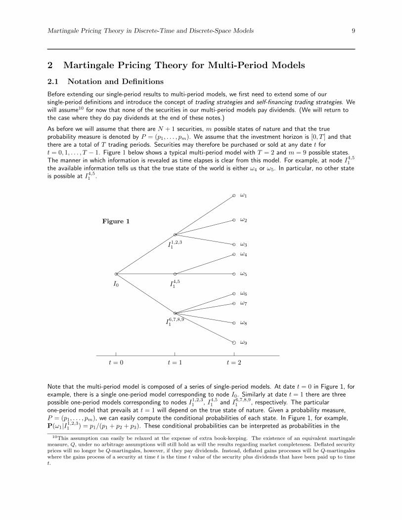
As before we will assume that there are N + 1 securities, m possible states of nature and that the trueprobability measure is denoted by P = (p1, . . . , pm). We assume that the investment horizon is [0, T ] and thatthere are a total of T trading periods. Securities may therefore be purchased or sold at any date t fort = 0, 1, . . . , T − 1. Figure 1 below shows a typical multi-period model with T = 2 and m = 9 possible states.The manner in which information is revealed as time elapses is clear from this model. For example, at node I4,51
the available information tells us that the true state of the world is either ω4 or ω5. In particular, no other stateis possible at I4,51 .
Figure 1
t = 0 t = 1 t = 2
c���������
QQQQQQQQQ
I0
���������
c���������hhhhhhhhhI1,2,31
����
����
�
cI4,51
((((((((
(chhhhhhhhhHHHH
HHHHH
����
����
�
I6,7,8,91
c ω1
c ω2
c ω3c ω4
c ω5
c ω6c ω7
c ω8
d ω9
Note that the multi-period model is composed of a series of single-period models. At date t = 0 in Figure 1, forexample, there is a single one-period model corresponding to node I0. Similarly at date t = 1 there are threepossible one-period models corresponding to nodes I1,2,31 , I4,51 and I6,7,8,91 , respectively. The particularone-period model that prevails at t = 1 will depend on the true state of nature. Given a probability measure,P = (p1, . . . , pm), we can easily compute the conditional probabilities of each state. In Figure 1, for example,P(ω1|I1,2,31 ) = p1/(p1 + p2 + p3). These conditional probabilities can be interpreted as probabilities in the
10This assumption can easily be relaxed at the expense of extra book-keeping. The existence of an equivalent martingalemeasure, Q, under no arbitrage assumptions will still hold as will the results regarding market completeness. Deflated securityprices will no longer be Q-martingales, however, if they pay dividends. Instead, deflated gains processes will be Q-martingaleswhere the gains process of a security at time t is the time t value of the security plus dividends that have been paid up to timet.
Martingale Pricing Theory in Discrete-Time and Discrete-Space Models 10
corresponding single-period models. For example, p1 = P(I1,2,31 |I0) P(ω1|I1,2,31 ). This observation (applied torisk-neutral probabilities) will allow us to easily generalize our single-period results to multi-period models.
Trading Strategies and Self-Financing Trading Strategies
Definition 10 A predictable stochastic process is a process whose time t value, Xt say, is known at timet− 1 given all the information that is available at time t− 1.
Definition 11 A trading strategy is a vector, θt = [θ(0)t (ω) . . . θ
(N)t (ω)]>, of predictable stochastic
processes that describes the number of units of each security held just before trading at time t, as a function oft and ω.
For example, θ(i)t (ω) is the number of units of the ith security held11 between times t− 1 and t in state ω. We
will sometimes write θ(i)t , omitting the explicit dependence on ω. Note that θt is known at date t− 1 as we
insisted in Definition 11 that θt be predictable. In our financial context, ‘predictable’ means that θt cannotdepend on information that is not yet available at time t− 1.
Example 8 (Constraints Imposed by Predictability of Trading Strategies)Referring to Figure 1, it must be the case that for all i = 0, . . . , N ,
θ(i)2 (ω1) = θ
(i)2 (ω2) = θ
(i)2 (ω3)
θ(i)2 (ω4) = θ
(i)2 (ω5)
θ(i)2 (ω6) = θ
(i)2 (ω7) = θ
(i)2 (ω8) = θ
(i)2 (ω9).
Exercise 6 What can you say about the relationship between the θ(i)1 (ωj)’s for j = 1, . . . ,m?
Definition 12 The value process, Vt(θ), associated with a trading strategy, θt, is defined by
Vt =
∑Ni=0 θ
(i)1 S
(i)0 for t = 0∑N
i=0 θ(i)t S
(i)t for t ≥ 1.
Definition 13 A self-financing trading strategy is a strategy, θt, where changes in Vt are due entirely totrading gains or losses, rather than the addition or withdrawal of cash funds. In particular, a self-financingstrategy satisfies
Vt =
N∑i=0
θ(i)t+1S
(i)t for t = 1, . . . , T − 1.
Definition 13 states that the value of a self-financing portfolio just before trading or re-balancing is equal to thevalue of the portfolio just after trading, i.e., no additional funds have been deposited or withdrawn.
Exercise 7 Show that if a trading strategy, θt, is self-financing then the corresponding value process, Vt,satisfies
Vt+1 − Vt =
N∑i=0
θ(i)t+1
(S(i)t+1 − S
(i)t
). (6)
Clearly then changes in the value of the portfolio are due to capital gains or losses and are not due to theinjection or withdrawal of funds. Note that we can also write (6) as
dVt = θ>t dSt,
which anticipates our continuous-time definition of a self-financing trading strategy.
We can now extend the one-period definitions of arbitrage opportunities, attainable claims and completeness.
11If θ(i)t is negative then it corresponds to the number of units sold short.
Martingale Pricing Theory in Discrete-Time and Discrete-Space Models 11
Arbitrage
Definition 14 A type A arbitrage opportunity is a self-financing trading strategy, θt, such that V0(θ) < 0and VT (θ) = 0. Similarly, a type B arbitrage opportunity is a self-financing trading strategy, θt, such thatV0(θ) = 0, VT (θ) ≥ 0 and EP0 [VT (θ)] > 0.
Attainability and Complete Markets
Definition 15 A contingent claim, C, is a random variable whose value at time T is known at that timegiven the information available then. It can be interpreted as the time T value of a security (or, depending onthe context, the time t value if this value is known by time t < T ).
Definition 16 We say that the contingent claim C is attainable if there exists a self-financing tradingstrategy, θt, whose value process, VT , satisfies VT = C.
Note that the value of the claim, C, in Definition 16 must equal the initial value of the replicating portfolio, V0,if there are no arbitrage opportunities available. We can now extend our definition of completeness.
Definition 17 We say that the market is complete if every contingent claim is attainable. Otherwise themarket is said to be incomplete.
Note that the above definitions of attainability and (in)completeness are consistent with our definitions forsingle-period models. With our definitions of a numeraire security and the cash account remaining unchanged,we can now define what we mean by an equivalent martingale measure (EMM), or set of risk-neutralprobabilities.
Equivalent Martingale Measures (EMMs)
We assume again that we have in mind a specific numeraire security with price process, S(n)t .
Definition 18 An equivalent martingale measure (EMM), Q = (q1, . . . , qm), is a set of probabilitiessuch that
1. qi > 0 for all i = 1, . . . ,m.
2. The deflated security prices are martingales. That is
S(i)
t :=S(i)t
S(n)t
= EQt
[S(i)t+s
S(n)t+s
]=: EQt
[S(i)
t+s
]for s, t ≥ 0, for all i = 0, . . . , N , and where EQt [.] denotes the expectation under Q conditional oninformation available at time t. (We also refer to Q as a set of risk-neutral probabilities.)
2.2 Pricing in Multi-Period Models
We will now generalize the results for single-period models to multi-period models. This is easily done using oursingle-period results and requires very little extra work.
Absence of Arbitrage ≡ Existence of EMM
We begin with two propositions that enable us to generalize Proposition 1.
Proposition 8 If an equivalent martingale measure, Q, exists, then the deflated value process, Vt, of anyself-financing trading strategy is a Q-martingale.

Martingale Pricing Theory in Discrete-Time and Discrete-Space Models 12
Proof: Let θt be the self-financing trading strategy and let V t+1 := Vt+1/S(n)t+1 denote the deflated value
process. We then have
EQt[V t+1
]= EQt
[N∑i=0
θ(i)t+1S
(i)
t+1
]
=
N∑i=0
θ(i)t+1EQt
[S(i)
t+1
]=
N∑i=0
θ(i)t+1S
(i)
t
= V t
demonstrating that V t is indeed a martingale, as claimed.
Remark 4 Note that Proposition 8 implies that the deflated price of any attainable security can be computedas the Q-expectation of the terminal deflated value of the security.
Proposition 9 If an equivalent martingale measure, Q, exists, then there can be no arbitrage opportunities.
Proof: The proof follows almost immediately from Proposition 8.
We can now now state our principal result for multi-period models, assuming as usual that a numeraire securityexists.
Theorem 10 (Fundamental Theorem of Asset Pricing: Part 1)
In the multi-period model there is no arbitrage if and only if there exists an EMM, Q.
Proof: (i) Suppose first that there is no arbitrage as defined by Definition 14. Then we can easily argue thereis no arbitrage (as defined by Definition 4) in any of the embedded one-period models. Theorem 5 then impliesthat each of the the embedded one-period models has a set of risk-neutral probabilities. By multiplying theseprobabilities as described in the paragraph immediately following Figure 1, we can construct an EMM, Q, asdefined by Definition 18.
(ii) Suppose there exists an EMM, Q. Then Proposition 9 gives the result.
Complete Markets ≡ Unique EMM
As was the case with single-period models, it is also true that multi-period models are complete if and only ifthe EMM is unique. (We are assuming here that there is no arbitrage so that an EMM is guaranteed to exist.)
Proposition 11 The market is complete if and only if every embedded one-period model is complete.
Exercise 8 Prove Proposition 11
We have the following theorem.
Theorem 12 (Fundamental Theorem of Asset Pricing: Part 2)
Assume there exists a security with strictly positive price process and that there are no arbitrage opportunities.Then the market is complete if and only if there exists exactly one risk-neutral martingale measure, Q.
Proof: (i) Suppose the market is complete. Then by Proposition 11 every embedded one-period model iscomplete so we can apply Theorem 7 to show that the EMM, Q, (which must exist since there is no arbitrage)is unique.
(ii) Suppose now Q is unique. Then the risk-neutral probability measure corresponding to each one-periodmodel is also unique. Now apply Theorem 7 again to obtain that the multi-period model is complete.
Martingale Pricing Theory in Discrete-Time and Discrete-Space Models 13
State Prices
As in the single-period models, we also have an equivalence between equivalent martingale measures, Q, and
sets of state prices. We will use π{t+s}t (Λ) to denote the time t price of a security that pays $1 at time t+ s in
the event that ω ∈ Λ. We are implicity assuming that we can tell at time t+ s whether or not ω ∈ Λ. In Figure
1, for example, π{1}0 (ω4, ω5) is a valid expression whereas π
{1}0 (ω4) is not.
2.3 Why is Absence of Arbitrage ≡ Existence of an EMM ?
Let us now develop some intuition for why the discounted price process, Stj/Sti , should be a Q-martingale if
there are no arbitrage opportunities. First, it is clear that we should not expect a non-deflated price process tobe a martingale under the true probability measure, P . After all, if a cash account is available, then it willalways grow in value as long as the risk-free rate of interest is positive. It cannot therefore be a P -martingale.
It makes sense then that we should compare the price processes of securities relative to one another rather thanexamine them on an absolute basis. This is why we deflate by some positive security. Even after deflating,however, it is still not reasonable to expect deflated price processes to be P -martingales. After all, somesecurities are riskier than others and since investors are generally risk averse it makes sense that riskier securitiesshould have higher expected rates of return. However, if we change to an equivalent martingale measure, Q,where probabilities are adjusted to reflect the riskiness of the various states, then we can expect deflated priceprocesses to be martingales under Q. The vital point here is that each qk must be strictly positive since we haveassumed that each pk is strictly positive.
As a further aid to developing some intuition, we might consider the following three scenarios:
Scenario 1
Imagine a multi-period model with two assets, both of whose price processes, Xt and Yt say, aredeterministic and positive. Convince yourself that in this model it must be the case that Xt/Yt is amartingale if there are to be no arbitrage opportunities. (A martingale in a deterministic model mustbe a constant process. Moreover, in a deterministic model a risk-neutral measure, Q, must coincidewith the true probability measure, P .)
Scenario 2
Generalize scenario 1 to a deterministic model with n assets, each of which has a positive price process.Note that you can choose to deflate by any process you choose. Again it should be clear that deflatedsecurity price processes are (deterministic) martingales.
Scenario 3
Now consider a one period stochastic model that runs from date t = 0 to date t = 1. There are only
two possible outcomes at date t = 1 and we assume there are only two assets, S(1)t and S
(2)t . Again,
convince yourself that if there are to be no arbitrage opportunities, then it must be the case that there
is probability measure, Q, such that S(1)t /S
(2)t is a Q-martingale. Of course we have already given a
proof of this result (and much more), but it helps intuition to look at this very simple case and seedirectly why an EMM must exist if there is no arbitrage.
Once these simple cases are understood, it is no longer surprising that the result (equivalence of absence ofarbitrage and existence of an EMM) extends to multiple periods, multiple assets and even continuous time. Youcan also see that the numeraire asset can actually be any asset with a strictly positive price process. Of coursewe commonly deflate by the cash account in practice as it is often very convenient to do so, but it is importantto note that our results hold if we deflate by other positive price processes. We now consider some examplesthat will use the various concepts and results that we have developed.
Martingale Pricing Theory in Discrete-Time and Discrete-Space Models 14
3 Examples
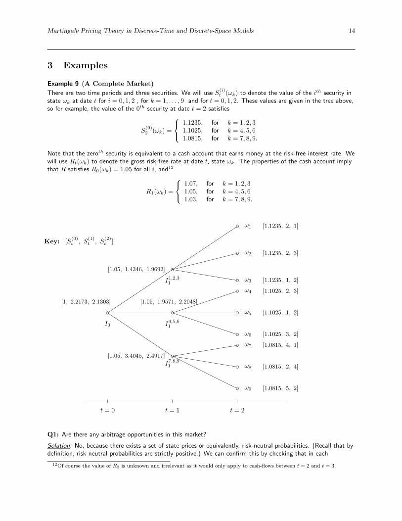
Example 9 (A Complete Market)
There are two time periods and three securities. We will use S(i)t (ωk) to denote the value of the ith security in
state ωk at date t for i = 0, 1, 2 , for k = 1, . . . , 9 and for t = 0, 1, 2. These values are given in the tree above,so for example, the value of the 0th security at date t = 2 satisfies
S(0)2 (ωk) =
1.1235, for k = 1, 2, 31.1025, for k = 4, 5, 61.0815, for k = 7, 8, 9.
Note that the zeroth security is equivalent to a cash account that earns money at the risk-free interest rate. Wewill use Rt(ωk) to denote the gross risk-free rate at date t, state ωk. The properties of the cash account implythat R satisfies R0(ωk) = 1.05 for all i, and12
R1(ωk) =
1.07, for k = 1, 2, 31.05, for k = 4, 5, 61.03, for k = 7, 8, 9.
t = 0 t = 1 t = 2
c[1, 2.2173, 2.1303]
����������
QQQQQQQQQQ
I0
����������
c[1.05, 1.4346, 1.9692] ������
����
hhhhhhhhhhI1,2,31
����
����
��
c[1.05, 1.9571, 2.2048]
PPPPPPPPPP
I4,5,61
((((((((
((c[1.05, 3.4045, 2.4917] hhhhhhhhhhHHHH
HHHHHH
I7,8,91
c ω1 [1.1235, 2, 1]
c ω2 [1.1235, 2, 3]
c ω3 [1.1235, 1, 2]c ω4 [1.1025, 2, 3]
c ω5 [1.1025, 1, 2]
c ω6 [1.1025, 3, 2]c ω7 [1.0815, 4, 1]
c ω8 [1.0815, 2, 4]
c ω9 [1.0815, 5, 2]
Key: [S(0)t , S
(1)t , S
(2)t ]
Q1: Are there any arbitrage opportunities in this market?
Solution: No, because there exists a set of state prices or equivalently, risk-neutral probabilities. (Recall that bydefinition, risk neutral probabilities are strictly positive.) We can confirm this by checking that in each
12Of course the value of R2 is unknown and irrelevant as it would only apply to cash-flows between t = 2 and t = 3.
Martingale Pricing Theory in Discrete-Time and Discrete-Space Models 15
embedded one-period model there is a strictly positive solution to St = πtSt+1 where St is the vector of securityprices at a particular time t node and St+1 is the matrix of date t = 1 prices at the successor nodes.
Q2: If not, is this a complete or incomplete market?
Solution: Complete, because we have a unique set of state prices or equivalently a unique equivalent martingalemeasure. We can check this by confirming that each embedded one-period model has a payoff matrix of fullrank.
Q3: Compute the state prices in this model.
Solution: First compute (how?) the prices at date 1 of $1 to be paid in each of the terminal states at date 2.
These are the state prices at date 1, π{2}1 , and we find
π{2}1 (ω1) = .2 , π
{2}1 (ω2) = .3 and π
{2}1 (ω3) = 0.4346 at I1,2,31
π{2}1 (ω4) = .3 , π
{2}1 (ω5) = .3 and π
{2}1 (ω6) = 0.3524 at I4,5,61
π{2}1 (ω7) = .25 , π
{2}1 (ω8) = .4 and π
{2}1 (ω9d) = 0.3209 at I7,8,91
The value at date 0 of $1 at nodes I1,2,31 , I4,5,61 and I7,8,91 , respectively, is given by
π{1}0 (I1,2,31 ) = .3 , π
{1}0 (I4,5,61 ) = .3 and π
{1}0 (I7,8,91 ) = .3524.
Therefore the state prices at date t = 0 are (why?)
π{2}0 (ω1) = .06, π
{2}0 (ω2) = .09, π
{2}0 (ω3) = 0.1304, π
{2}0 (ω4) = .09, π
{2}0 (ω5) = .09
π{2}0 (ω6) = 0.1057, π
{2}0 (ω7) = 0.0881, π
{2}0 (ω8) = 0.1410, π
{2}0 (ω9) = 0.1131.
We can easily check that these state prices do indeed correctly price (subject to rounding errors) the threesecurities at date t = 0.
Q4: Compute the risk-neutral or martingale probabilities when we discount by the cash account, i.e., the zeroth
security.
Solution: When we deflate by the cash account the risk-neutral probabilities for the nine possible paths at time0 may be computed using the expression
qk =π{2}0 (ωk)S
(0)2 (ωk)∑
π{2}0 (ωj)S
(0)2 (ωj)
. (7)
We have not shown that the expression in (7) is in fact correct, though note that it generalizes the one-periodexpression in (4).
Exercise 9 Check that (7) is indeed correct. (You may do this by deriving it in exactly the same manner as(4). Alternatively, it may be derived by using equation (4) to compute the risk-neutral probabilities of theembedded one-period models and multiplying them appropriately to obtain the qk’s. Note that the risk-neutralprobabilities in the one-period models are conditional risk-neutral probabilities of the multi-period model.)
We therefore have
q1 q2 q3 q4 q5 q6 q7 q8 q90.0674 0.1011 0.1465 0.0992 0.0992 0.1165 0.0953 0.1525 0.1223

Martingale Pricing Theory in Discrete-Time and Discrete-Space Models 16
Q5: Compute the risk-neutral probabilities (i.e. the martingale measure) when we discount by the secondsecurity.
Solution: Similarly, when we deflate by the second asset, the risk-neutral probabilities are given by:
q1 q2 q3 q4 q5 q6 q7 q8 q90.0282 0.1267 0.1224 0.1267 0.0845 0.0992 0.0414 0.2647 0.1062
Q6: Using the state prices, find the price of a call option on the the first asset with strike k = 2 and expirationdate t = 2.
Solution: The payoffs of the call option and the state prices are given by:
State 1 2 3 4 5 6 7 8 9
Payoff 0 0 0 0 0 1 2 0 3State Price .06 .09 .1304 .09 .09 .1057 .0881 .1410 .1131
The price of the option is therefore (why?) given by .1057 + (2× .0881) + (3× .1131) = .6212.
Q7: Confirm your answer in (6) by recomputing the option price using the martingale measure of (5).
Solution: Using the risk-neutral probabilities when we deflate by the second asset we have:
State 1 2 3 4 5 6 7 8 9
Deflated Payoff 0 0 0 0 0 1/2 2/1 0 3/2Risk-Neutral Probabilities 0.0282 0.1267 0.1224 0.1267 0.0845 0.0992 0.0414 0.2647 0.1062
The price of the option deflated by the initial price of the second asset is therefore given by(.0992× .5) + (2× .0414) + (3/2)× .1062 = .2917. And so the option price is given by .2917× 2.1303 = .6214,which is the same answer (modulo rounding errors) as we obtained in (6).
In Example 9 we computed the option price by working directly from the date t = 2 payoffs to the date t = 0price. Another method for pricing derivative securities is to iterate the price backwards through the tree. That iswe first compute the price at the date t = 1 nodes and then use the date t = 1 price to compute the date t = 0price. This technique of course, is also implemented using the risk-neutral probabilities or equivalently, the stateprices.
Exercise 10 Repeat Question 6 of Example 9, this time using dynamic programming to compute the optionprice.
Remark 5 While Rt was stochastic in Example 9, we still refer to it as a risk-free interest rate. Thisinterpretation is valid since we know for certain at date i the date i+ 1 value of $1 invested in the cash accountat date i.
Martingale Pricing Theory in Discrete-Time and Discrete-Space Models 17
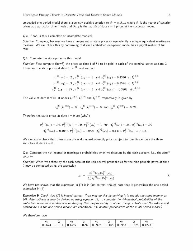
Example 10 (An Incomplete Market)Consider the same tree as in Example 9 only now state ω6 is a successor state to node I6,7,8,91 instead of nodeI4,51 . We have also changed the payoff of the zeroth asset in this state so that our interpretation of the thezeroth asset as a cash account remains appropriate. The new tree is displayed below:
t = 0 t = 1 t = 2
c[1, 2.2173, 2.1303]
����������
QQQQQQQQQQ
I0
����������
c[1.05, 1.4346, 1.9692] ������
����
hhhhhhhhhhI1,2,31
����
����
��
c[1.05, 1.9571, 2.2048]
I4,51
(((((((
(((c[1.05, 3.4045, 2.4917] hhhhhhhhhhHH
HHHHHH
HH
����
����
��
I6,7,8,91
c ω1 [1.1235, 2, 1]
c ω2 [1.1235, 2, 3]
c ω3 [1.1235, 1, 2]c ω4 [1.1025, 2, 3]
c ω5 [1.1025, 1, 2]
c ω6 [1.0815, 3, 2]c ω7 [1.0815, 4, 1]
c ω8 [1.0815, 2, 4]
c ω9 [1.0815, 5, 2]
Key: [S(0)t , S
(1)t , S
(2)t ]
Q1: Is this model arbitrage free?
Solution: We know the absence of arbitrage is equivalent to the existence of positive state prices or, equivalently,risk-neutral probabilities. Moreover, if the model is arbitrage free then so is every one-period sub-market so allwe need to do is see if we can construct positive state prices for each of the four one-period markets representedby the nodes I1,2,31 , I4,51 , I6,7,8,91 and I0.
First, it is clear that the one-period market beginning at I1,2,31 is arbitrage-free since this is the same as thecorresponding one-period model in Example 9. For the subproblem beginning at I6,7,8,91 we can take (check)
[π{2}1 (ω6) π
{2}1 (ω7) π
{2}1 (ω8) π
{2}1 (ω9)] = [0.0737 0.1910 0.3705 0.3357] so this sub-market is also arbitrage
free. (Note that other vectors will also work.)
However, it is not possible to find a state price vector, [π{2}1 (ω4) π
{2}1 (ω5)], for the one-period market beginning
at I4,51 . In particular, this implies there is an arbitrage opportunity there and so we can conclude13 that themodel is not arbitrage-free.
Q2: Suppose the prices of the three securities were such that there were no arbitrage opportunities. Withoutbothering to compute such prices, do you think the model would then be a complete or incomplete model?
Solution: The model is incomplete as the rank of the payoff matrix in the one-period model beginning at I6,7,8,91
13You can check the one-period model beginning at node I0 if you like!
Martingale Pricing Theory in Discrete-Time and Discrete-Space Models 18
is less than 4.
Q3: Suppose again that the security prices were such that there were no arbitrage opportunities. Give a simpleargument for why forward contracts are attainable. (We can therefore price them in this model.)
Solution: This is left as an exercise. (However we will return to this issue and the pricing of futures contracts inSection 5.2.)
Exercise 11 Find an arbitrage opportunity in the one-period model beginning at node I4,51 in Example 10.
4 Dividends and Intermediate Cash-Flows
Thus far, we have assumed that none of the securities pay intermediate cash-flows. An example of such asecurity is a dividend-paying stock. This is not an issue in the single period models since any such cash-flows arecaptured in the date t = 1 value of the securities. For multi-period models, however, we sometimes need toexplicitly model these intermediate cash payments. All of the results that we have derived in these notes still gothrough, however, as long as we make suitable adjustments to our price processes and are careful with ourbookkeeping. In particular, deflated cumulative gains processes rather than deflated security prices are nowQ-martingales. The cumulative gain process, Gt, of a security at time t is equal to value of the security at timet plus accumulated cash payments that result from holding the security.
Consider our discrete-time, discrete-space framework where a particular security pays dividends. Then if themodel is arbitrage-free there exists an EMM, Q, such that
St = EQt
t+s∑j=t+1
Dj + St+s
where Dj is the time j dividend that you receive if you hold one unit of the security, and St is its time tex-dividend price. This result is easy to derive using our earlier results. All we have to do is view eachdividend as a separate security with St then interpreted as the price of the portfolio consisting of these individualsecurities as well as a security that is worth St+s at date t+ s. The definitions of complete and incompletemarkets are unchanged and the associated results we derived earlier still hold when we also account for thedividends in the various payoff matrices. For example, if θt is a self-financing strategy in a model with dividendsthen Vt, the corresponding value process, should satisfy
Vt+1 − Vt =
N∑i=0
θ(i)t+1
(S(i)t+1 +D
(i)t+1 − S
(i)t
). (8)
Note that the time t dividends, D(i)t , do not appear in (8) since we assume that Vt is the value of the portfolio
just after dividends have been paid. This interpretation is consistent with taking St to be the time t ex-dividendprice of the security.
The various definitions of complete and incomplete markets, state prices, arbitrage etc. are all unchanged whensecurities can pay dividends. As mentioned earlier, the First Fundamental Theorem of Asset Pricing now statesthat deflated cumulative gains processes rather than deflated security prices are now Q-martingales. The secondfundamental theorem goes through unchanged.
4.1 Using a Dividend-Paying Security as the Numeraire
Until now we have always assumed that the numeraire security does not pay any dividends. If a security paysdividends then we cannot use it as a numeraire. Instead we can use the security’s cumulative gains process as
Martingale Pricing Theory in Discrete-Time and Discrete-Space Models 19
the numeraire as long as this gains process is strictly positive. This makes intuitive sense as it is the gainsprocess that represents the true value dynamics of holding the security.
In continuous-time models of equities it is common to assume that the equity pays a continuous dividend yieldof q so that qStdt represent the dividend paid in the time interval (t, t+ dt]. The cumulative gains processcorresponding to this stock price is then Gt := eqtSt and it is this quantity that can be used as a numeraire.
5 Applications of Martingale Pricing
We now consider applying what we know about martingale pricing to the binomial model as well as the generalpricing of forwards and futures.
5.1 Pricing in the Binomial Model
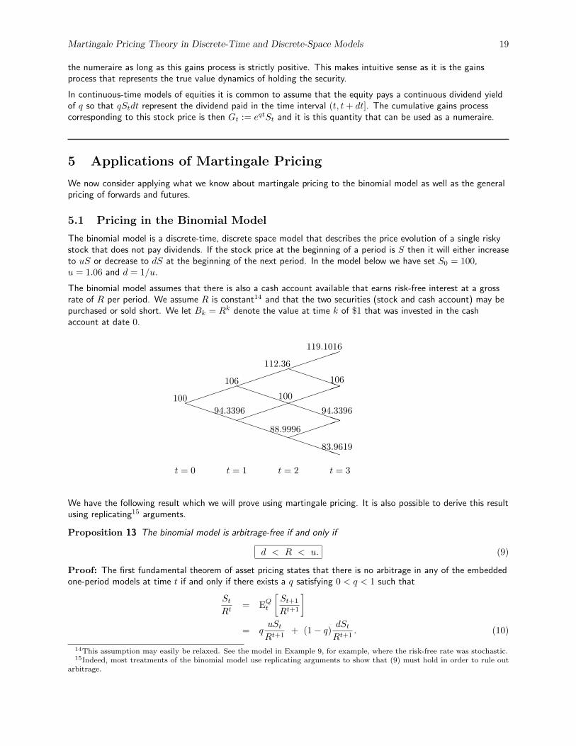
The binomial model is a discrete-time, discrete space model that describes the price evolution of a single riskystock that does not pay dividends. If the stock price at the beginning of a period is S then it will either increaseto uS or decrease to dS at the beginning of the next period. In the model below we have set S0 = 100,u = 1.06 and d = 1/u.
The binomial model assumes that there is also a cash account available that earns risk-free interest at a grossrate of R per period. We assume R is constant14 and that the two securities (stock and cash account) may bepurchased or sold short. We let Bk = Rk denote the value at time k of $1 that was invested in the cashaccount at date 0.
����
����
����
�����
PPPPPPPPPPPPPPPPP
PPPPPPPPPPPP����
����
����
PPPPPP
����
��
t = 0 t = 1 t = 2 t = 3
100
106
112.36
119.1016
100
106
94.3396 94.3396
88.9996
83.9619
We have the following result which we will prove using martingale pricing. It is also possible to derive this resultusing replicating15 arguments.
Proposition 13 The binomial model is arbitrage-free if and only if
d < R < u. (9)
Proof: The first fundamental theorem of asset pricing states that there is no arbitrage in any of the embeddedone-period models at time t if and only if there exists a q satisfying 0 < q < 1 such that
StRt
= EQt
[St+1
Rt+1
]= q
uStRt+1
+ (1− q) dStRt+1
. (10)
14This assumption may easily be relaxed. See the model in Example 9, for example, where the risk-free rate was stochastic.15Indeed, most treatments of the binomial model use replicating arguments to show that (9) must hold in order to rule out
arbitrage.
Martingale Pricing Theory in Discrete-Time and Discrete-Space Models 20
Solving (10), we find that q = (R− d)/(u− d) and 1− q = (u−R)/(u− d). The result now follows sinceeach of the embedded one-period models in the binomial model are identical.
Note that the q we obtained in the above Proposition was both unique and node independent. Therefore thebinomial model itself is arbitrage-free and complete16 if (9) is satisfied and we will always assume this to be thecase. We will usually use the cash account, Bk, as the numeraire security so that the price of any security canbe computed as the discounted expected payoff of the security under Q. Thus the time t price of a security17
that is worth XT at time T (and does not provide any cash flows in between) is given by
Xt = Bt EQt
[XT
BT
]=
1
RT−tEQt [XT ]. (11)
The binomial model is one of the workhorses of financial engineering. In addition to being a complete model, itis also recombining. For example, an up-move followed by a down-move leads to the same node as a down-movefollowed by an up-move. This recombining feature implies that the number of nodes in the tree grows linearlywith the number of time periods rather than exponentially. This leads to a considerable gain in computationalefficiency when it comes to pricing path-independent securities.
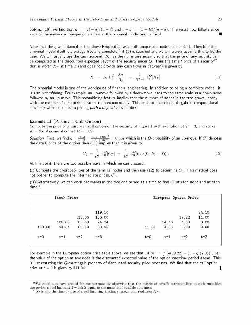
Example 11 (Pricing a Call Option)Compute the price of a European call option on the security of Figure 1 with expiration at T = 3, and strikeK = 95. Assume also that R = 1.02.
Solution: First, we find q = R−du−d = 1.02−1.06−1
1.6−1.06−1 = 0.657 which is the Q-probability of an up-move. If C0 denotesthe date 0 price of the option then (11) implies that it is given by
C0 =1
R3EQ0 [CT ] =
1
R3EQ0 [max(0, S3 − 95)]. (12)
At this point, there are two possible ways in which we can proceed:
(i) Compute the Q-probabilities of the terminal nodes and then use (12) to determine C0. This method doesnot bother to compute the intermediate prices, Ct.
(ii) Alternatively, we can work backwards in the tree one period at a time to find Ct at each node and at eachtime t.
Stock Price European Option Price
119.10 24.10
112.36 106.00 19.22 11.00
106.00 100.00 94.34 14.76 7.08 0.00
100.00 94.34 89.00 83.96 11.04 4.56 0.00 0.00
t=0 t=1 t=2 t=3 t=0 t=1 t=2 t=3
For example in the European option price table above, we see that 14.76 = 1R (q(19.22) + (1− q)(7.08)), i.e.,
the value of the option at any node is the discounted expected value of the option one time period ahead. Thisis just restating the Q-martingale property of discounted security price processes. We find that the call optionprice at t = 0 is given by $11.04.
16We could also have argued for completeness by observing that the matrix of payoffs corresponding to each embeddedone-period model has rank 2 which is equal to the number of possible outcomes.
17Xt is also the time t value of a self-financing trading strategy that replicates XT .
Martingale Pricing Theory in Discrete-Time and Discrete-Space Models 21
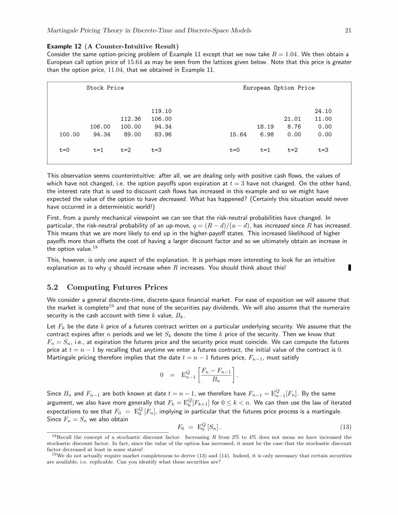
Example 12 (A Counter-Intuitive Result)Consider the same option-pricing problem of Example 11 except that we now take R = 1.04. We then obtain aEuropean call option price of 15.64 as may be seen from the lattices given below. Note that this price is greaterthan the option price, 11.04, that we obtained in Example 11.
Stock Price European Option Price
119.10 24.10
112.36 106.00 21.01 11.00
106.00 100.00 94.34 18.19 8.76 0.00
100.00 94.34 89.00 83.96 15.64 6.98 0.00 0.00
t=0 t=1 t=2 t=3 t=0 t=1 t=2 t=3
This observation seems counterintuitive: after all, we are dealing only with positive cash flows, the values ofwhich have not changed, i.e. the option payoffs upon expiration at t = 3 have not changed. On the other hand,the interest rate that is used to discount cash flows has increased in this example and so we might haveexpected the value of the option to have decreased. What has happened? (Certainly this situation would neverhave occurred in a deterministic world!)
First, from a purely mechanical viewpoint we can see that the risk-neutral probabilities have changed. Inparticular, the risk-neutral probability of an up-move, q = (R− d)/(u− d), has increased since R has increased.This means that we are more likely to end up in the higher-payoff states. This increased likelihood of higherpayoffs more than offsets the cost of having a larger discount factor and so we ultimately obtain an increase inthe option value.18
This, however, is only one aspect of the explanation. It is perhaps more interesting to look for an intuitiveexplanation as to why q should increase when R increases. You should think about this!
5.2 Computing Futures Prices
We consider a general discrete-time, discrete-space financial market. For ease of exposition we will assume thatthe market is complete19 and that none of the securities pay dividends. We will also assume that the numerairesecurity is the cash account with time k value, Bk.
Let Fk be the date k price of a futures contract written on a particular underlying security. We assume that thecontract expires after n periods and we let Sk denote the time k price of the security. Then we know thatFn = Sn, i.e., at expiration the futures price and the security price must coincide. We can compute the futuresprice at t = n− 1 by recalling that anytime we enter a futures contract, the initial value of the contract is 0.Martingale pricing therefore implies that the date t = n− 1 futures price, Fn−1, must satisfy
0 = EQn−1
[Fn − Fn−1
Bn
].
Since Bn and Fn−1 are both known at date t = n− 1, we therefore have Fn−1 = EQn−1[Fn]. By the same
argument, we also have more generally that Fk = EQk [Fk+1] for 0 ≤ k < n. We can then use the law of iterated
expectations to see that F0 = EQ0 [Fn], implying in particular that the futures price process is a martingale.Since Fn = Sn we also obtain
F0 = EQ0 [Sn] . (13)18Recall the concept of a stochastic discount factor. Increasing R from 2% to 4% does not mean we have increased the
stochastic discount factor. In fact, since the value of the option has increased, it must be the case that the stochastic discountfactor decreased at least in some states!
19We do not actually require market completeness to derive (13) and (14). Indeed, it is only necessary that certain securitiesare available, i.e. replicable. Can you identify what these securities are?
Martingale Pricing Theory in Discrete-Time and Discrete-Space Models 22
Exercise 12 What property of the cash account did we use in deriving (13)? (Note as a result that (13) onlyholds when Q is the EMM corresponding to taking the cash account as numeraire.)
Exercise 13 Does (13) change if the underlying security pays dividends? You can assume that Si is then theex-dividend price of the security at time i.
5.3 Computing Forward Prices
Now let us consider the date 0 price, G0, of a forward contract for delivery of the security at the same date,t = n. We recall that G0 is chosen in such a way that the contract is initially worth zero. In particular,martingale pricing implies
0 = EQ0
[Sn −G0
Bn
].
Rearranging terms and using the fact that G0 is known at date t = 0 we obtain
G0 =EQ0 [Sn/Bn]
EQ0 [1/Bn]. (14)
Remark 6 Note that (14) holds regardless of whether or not the underlying security pays dividends or couponsor whether there are costs associated with storing the security. (Storage costs may be viewed as negative
dividends.) Dividends (or other intermediate cash-flows) influence G0 through the evaluation of EQ0 [Sn/Bn].
Remark 7 If the underlying security does not pay dividends then we obtain G0 = S0/EQ0 [1/Bn]. This is
consistent with the expression, S/d(0, n), that was given in the Primer on Forwards, Futures and Swaps lecture
notes. This is clear since EQ0 [1/Bn] is the time 0 value of $1 at time n and this, by definition, is equal to d(0, n).
Exercise 14 If the underlying security does pay dividends (or have storage costs) then show that the expressionin (14) is consistent with the expression given in the Primer on Forwards, Futures and Swaps lecture notes.
We are also in a position now to identify when forwards and futures price coincide. In particular, if we compare(14) with (13) then we immediately obtain the following result.
Theorem 14 If Bn and Sn are Q-independent, then G0 = F0. In particular, if interest rates are deterministic,we have G0 = F0.
Corollary 1 In the binomial model with a constant (or deterministic) gross interest rate, R, we must haveG0 = F0.
Exercise 15 In practice, interest rates are stochastic and often tend to be positively correlated withmovements in the stock market. In such circumstances, convince yourself by considering (13) and (14) that thefutures price, F0, will generally be greater than the forward price, G0, when the underlying security is an equityindex such as the S&P500.
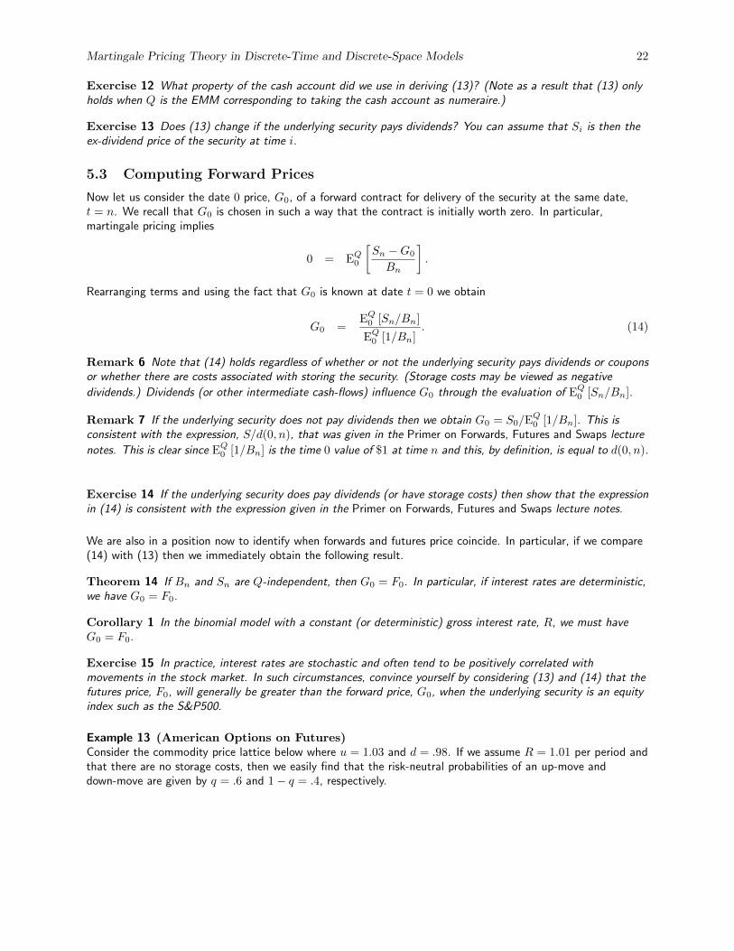
Example 13 (American Options on Futures)Consider the commodity price lattice below where u = 1.03 and d = .98. If we assume R = 1.01 per period andthat there are no storage costs, then we easily find that the risk-neutral probabilities of an up-move anddown-move are given by q = .6 and 1− q = .4, respectively.
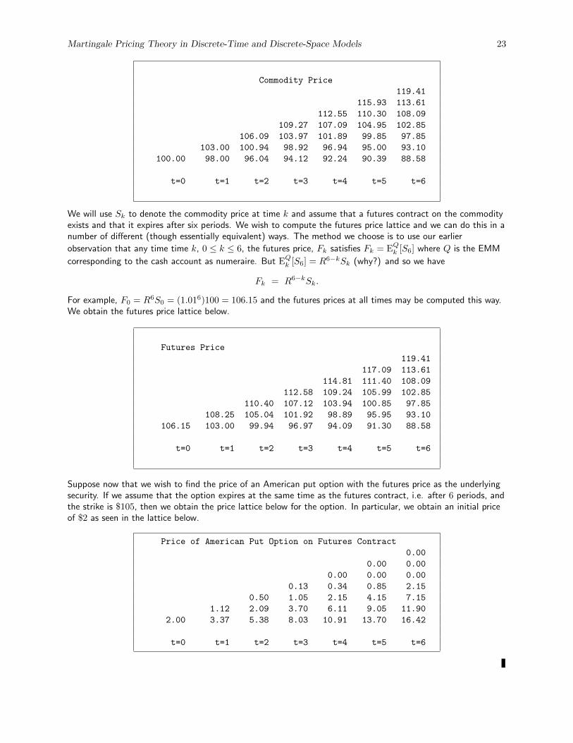
Martingale Pricing Theory in Discrete-Time and Discrete-Space Models 23
Commodity Price
119.41
115.93 113.61
112.55 110.30 108.09
109.27 107.09 104.95 102.85
106.09 103.97 101.89 99.85 97.85
103.00 100.94 98.92 96.94 95.00 93.10
100.00 98.00 96.04 94.12 92.24 90.39 88.58
t=0 t=1 t=2 t=3 t=4 t=5 t=6
We will use Sk to denote the commodity price at time k and assume that a futures contract on the commodityexists and that it expires after six periods. We wish to compute the futures price lattice and we can do this in anumber of different (though essentially equivalent) ways. The method we choose is to use our earlier
observation that any time time k, 0 ≤ k ≤ 6, the futures price, Fk satisfies Fk = EQk [S6] where Q is the EMM
corresponding to the cash account as numeraire. But EQk [S6] = R6−kSk (why?) and so we have
Fk = R6−kSk.
For example, F0 = R6S0 = (1.016)100 = 106.15 and the futures prices at all times may be computed this way.We obtain the futures price lattice below.
Futures Price
119.41
117.09 113.61
114.81 111.40 108.09
112.58 109.24 105.99 102.85
110.40 107.12 103.94 100.85 97.85
108.25 105.04 101.92 98.89 95.95 93.10
106.15 103.00 99.94 96.97 94.09 91.30 88.58
t=0 t=1 t=2 t=3 t=4 t=5 t=6
Suppose now that we wish to find the price of an American put option with the futures price as the underlyingsecurity. If we assume that the option expires at the same time as the futures contract, i.e. after 6 periods, andthe strike is $105, then we obtain the price lattice below for the option. In particular, we obtain an initial priceof $2 as seen in the lattice below.
Price of American Put Option on Futures Contract
0.00
0.00 0.00
0.00 0.00 0.00
0.13 0.34 0.85 2.15
0.50 1.05 2.15 4.15 7.15
1.12 2.09 3.70 6.11 9.05 11.90
2.00 3.37 5.38 8.03 10.91 13.70 16.42
t=0 t=1 t=2 t=3 t=4 t=5 t=6

Martingale Pricing Theory in Discrete-Time and Discrete-Space Models 24
Appendix A: Finding State Price Vectors
In Example 2 we saw that [π1 π2 π3 π4]> = [0.2433 0.1156 0.3140 0.3168]> was a vector of state prices forthe security market of that example. In particular, it satisfied S>1 π = S0, that is
1.03 1.03 1.03 1.033.00 4.00 2.00 5.002.00 1.00 4.00 2.00
0.24330.11560.31400.3168
=
1.01943.40452.4917
where S0 was the vector of date 0 security prices, and S>1 was the matrix of date 1 security prices. How did wefind such a vector π?
Consider the equation Ax = b where A is a known m× n matrix and b is a known m× 1 vector. We would liketo solve this equation for the vector x. There may be no solution, infinitely many solutions or a unique solution.If more than one solution exists so that Ax1 = Ax2 = b with x1 6= x2 then y := x1 − x2 is an element of thenullspace of A. That is Ay = 0. In particular, any solution to Ax = b can be written as the sum of a particularsolution, x1, and an element, w, of the nullspace.
How do we apply this to finding a vector of positive state prices, assuming such a vector exists. First try andfind a particular solution. In Matlab, for example, this can be done20 by using the matrix divide command “\”:
>> x1=S1’\S0
x1 =
0
0.3102
0.4113
0.2682
We then find the nullspace21 of S1> by using the “null” command:
>> w=null(S1’)
w =
0.7372
-0.5898
-0.2949
0.1474
Now every possible solution to S>1 π = S0 can be written asπ1π2π3π4
=
0
0.31020.41130.2682
+ ε
0.7372−0.5898−0.29490.1474
where ε is any real number. We just need to find an ε such that the solution is strictly positive. If no suchepsilon exists, then there is no vector of state prices. We chose ε = .33 in our example.
20The transpose of a matrix, A, in Matlab is A′.21The nullspace of a matrix is a vector space and the “null” command in Matlab will return a basis for this vector space. Any
element of the nullspace can then be written as a linear combination of elements in the basis. In our example, the dimensionalityof the nullspace is 1 and so there is only one element in the basis which we have denoted by ‘w’.
Martingale Pricing Theory in Discrete-Time and Discrete-Space Models 25
Appendix B: Optimal Stopping and Pricing American Options
An American option on a security gives the holder of the option the right to exercise it at any date on or beforethe expiration date, T . An exercise strategy, τ , is a rule specifying when the option should be exercised.Because τ can depend on the evolution of information in the model, it is in general a random variable. However,it should not be possible to base the decision to exercise or not on information that is not yet available. Wetherefore insist that τ is a stopping time.
Let Vt denote the date s price of an American option that expires at date T > t. The owner of the option mayexercise it any date s ∈ {t, . . . , T}. If exercised at time s, the owner of the option then receives Ys. We assumethat markets are complete and that there are no arbitrage opportunities so there exists a unique equivalentmartingale measure, Q, relative to some numeraire security, Bt. We want to determine an expression for Vt.
Theorem 15 (a) Let τ denote a generic stopping time and define
Zt := maxτ∈{t,...,T}
EQt
[YτBtBτ
]. (15)
Then Zt/Bt is the smallest supermartingale satisfying Zt ≥ Yt for all t. Moreover
τ∗(t) := min{s ≥ t : Zs = Ys} (16)
is an optimal stopping time for the optimization problem in (15). (Zt/Bt is known as the Snell Envelope ofYt/Bt.)
(b) The American option price, Vt, satisfies Vt = Zt for all t ∈ {0, . . . , T} and τ∗(0) is an optimal exercisestrategy.
Proof: (a) First note that ZT /BT = YT /BT . We can then use (15) and the tower property of conditionalexpectations to obtain
ZT−1BT−1
= max
{YT−1BT−1
, EQT−1
[ZTBT
]}.
More generally, we can use (15) to obtain
ZtBt
= max
{YtBt, maxτ≥t+1
EQt
[EQt+1
[YτBτ
]]}= max
{YtBt, EQt
[maxτ≥t+1
EQt+1
[YτBτ
]]}= max
{YtBt, EQt
[Zt+1
Bt+1
]}. (17)
It then follows22 from (17) that Zt/Bt is a supermartingale. Moreover, it is clear that Zt ≥ Yt. Now supposethat Ut/Bt is any other supermartingale satisfying Ut ≥ Yt. Since ZT = YT it is clear that ZT ≤ UT . Moreover,by hypothesis Ut−1 clearly satisfies
Ut−1Bt−1
≥ max
{Yt−1Bt−1
, EQt−1
[UtBt
]}.
Iterating backwards from t = T it is clear that Ut ≥ Zt.Finally, in order to prove that τ∗(t) is an optimal stopping time we argue as follows. Let τ̂(t) ≥ t be any optimalpolicy starting from time t so that Z
τ̂(t)= Y
τ̂(t)and τ̂(t) ≥ τ∗(t). But then
EQτ∗(t)
[Yτ̂(t)
Bτ̂(t)
]≤
Zτ∗(t)
Bτ∗(t)=
Yτ∗(t)
Bτ∗(t)
22Note that a simple dynamic programming argument could also be used to derive (17).
Martingale Pricing Theory in Discrete-Time and Discrete-Space Models 26
by (15) and (16). The law of iterated expectations now implies EQt
[Yτ̂(t)
Bτ̂(t)
]≤ EQt
[Yτ∗(t)
Bτ∗(t)
]and the result now
follows.
(b) Note that since markets are complete, we know that Yτ is attainable for every stopping time, τ . We need toconsider two situations: (i) Vt < Zt and (ii) Vt > Zt.
If (i) prevails, you should purchase the American option at a cost of Vt, adopt the optimal exercise policy, τ∗(t),of part (a) and adopt a self-financing trading strategy that is equivalent to selling the security with payoff Yτ∗(t)
at time τ∗(t). The initial income from this trading strategy is Zt − Vt and so this clearly leads to arbitrageprofits.
If (ii) prevails, you should sell the option and invest the proceeds appropriately to construct an arbitrage. Inparticular, you can adopt a super-replicating strategy that super-replicates the payoff at exercise regardless ofthe exercise policy that is used. The details are left as an exercise but the argument can be made rigorous23 byconstructing a self-financing strategy that replicates the martingale component of the Doob decomposition ofthe super-martingale Zt/Bt.
We can use the result of Theorem 15 and in particular, equation (17), to price American options. For example,in the binomial model we can use dynamic programming to compute the optimal strategy. As usual, we will usethe cash account (with value Bk at date k), as the numeraire security.
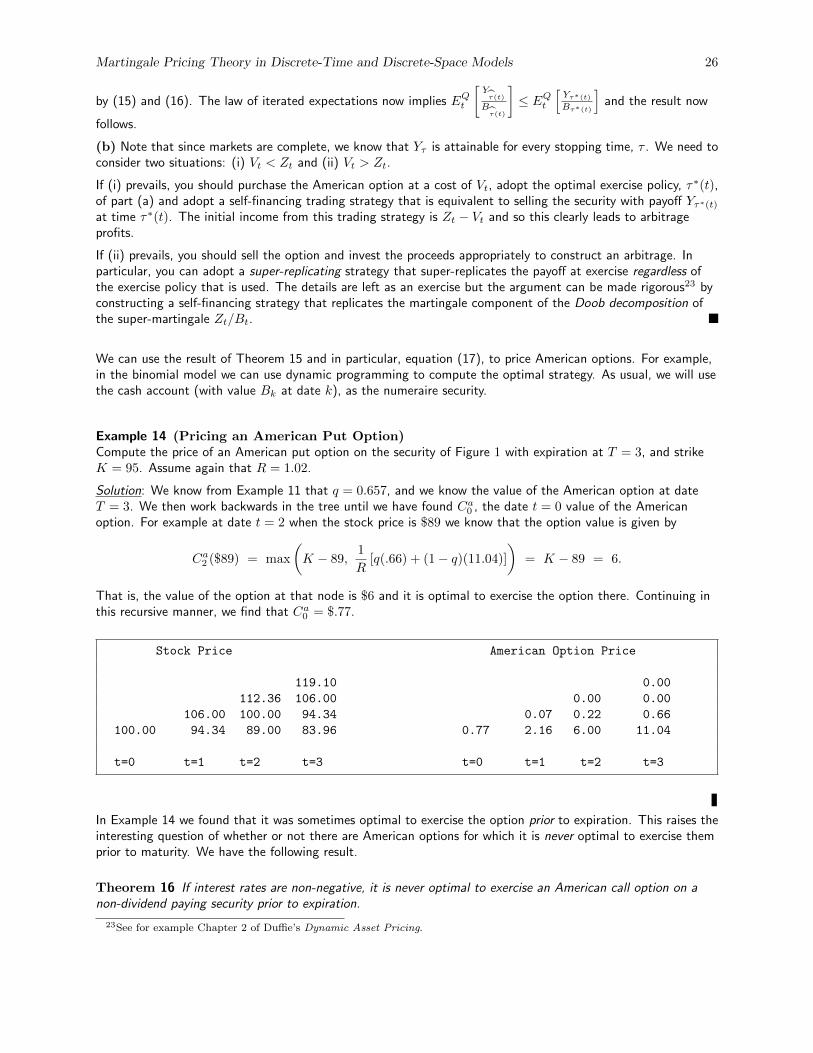
Example 14 (Pricing an American Put Option)Compute the price of an American put option on the security of Figure 1 with expiration at T = 3, and strikeK = 95. Assume again that R = 1.02.
Solution: We know from Example 11 that q = 0.657, and we know the value of the American option at dateT = 3. We then work backwards in the tree until we have found Ca0 , the date t = 0 value of the Americanoption. For example at date t = 2 when the stock price is $89 we know that the option value is given by
Ca2 ($89) = max
(K − 89,
1
R[q(.66) + (1− q)(11.04)]
)= K − 89 = 6.
That is, the value of the option at that node is $6 and it is optimal to exercise the option there. Continuing inthis recursive manner, we find that Ca0 = $.77.
Stock Price American Option Price
119.10 0.00
112.36 106.00 0.00 0.00
106.00 100.00 94.34 0.07 0.22 0.66
100.00 94.34 89.00 83.96 0.77 2.16 6.00 11.04
t=0 t=1 t=2 t=3 t=0 t=1 t=2 t=3
In Example 14 we found that it was sometimes optimal to exercise the option prior to expiration. This raises theinteresting question of whether or not there are American options for which it is never optimal to exercise themprior to maturity. We have the following result.
Theorem 16 If interest rates are non-negative, it is never optimal to exercise an American call option on anon-dividend paying security prior to expiration.
23See for example Chapter 2 of Duffie’s Dynamic Asset Pricing.
Martingale Pricing Theory in Discrete-Time and Discrete-Space Models 27
Proof: Using the Q-martingale property of the deflated security price process and the non-negativity of interestrates, we have
EQt
[(St+s/Bt+s − K/Bt+s)
+]≥ EQt [St+s/Bt+s − K/Bt+s]
= St/Bt − KEQt [1/Bt+s]
≥ St/Bt − K/Bt.
Since it is also the case that (St+s/Bt+s − K/Bt+s)+ ≥ 0, we therefore also have
EQt
[(St+s/Bt+s − K/Bt+s)
+]≥ (St/Bt − K/Bt)
+.
That is, (St/Bt − K/Bt)+ is a sub-martingale. Now the Optional Sampling Theorem for sub-martingales
states that if Yt is a sub-martingale and τ ≤ T is a stopping time, then EQ0 [Yτ ] ≤ EQ0 [YT ]. If we apply thisresult to (St/Bt − K/Bt)
+ and recall that the price, Ca0 , of the American option is given by
Ca0 = maxτ
EQ0
[(Sτ/Bτ − K/Bτ )
+]
we see that Ca0 = EQ0
[(ST /BT − K/BT )
+]
and it is never optimal to exercise early.
Remark 8 Note that if the security paid dividends in [0, T ], then St/Bt would not be a Q-martingale and theabove proof would not go through. The result generalizes to other types of American options where theunderlying security, St, again does not pay dividends in [0, T ], and where the payoff function is a convexfunction of S. The proof is similar and relies on the application of Jensen’s Inequality.
Martingale Pricing Theory in Discrete-Time and Discrete-Space Models 28
Exercises
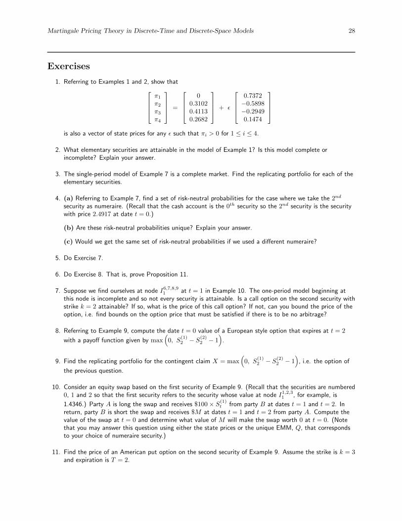
1. Referring to Examples 1 and 2, show thatπ1π2π3π4
=
0
0.31020.41130.2682
+ ε
0.7372−0.5898−0.29490.1474
is also a vector of state prices for any ε such that πi > 0 for 1 ≤ i ≤ 4.
2. What elementary securities are attainable in the model of Example 1? Is this model complete orincomplete? Explain your answer.
3. The single-period model of Example 7 is a complete market. Find the replicating portfolio for each of theelementary securities.
4. (a) Referring to Example 7, find a set of risk-neutral probabilities for the case where we take the 2nd
security as numeraire. (Recall that the cash account is the 0th security so the 2nd security is the securitywith price 2.4917 at date t = 0.)
(b) Are these risk-neutral probabilities unique? Explain your answer.
(c) Would we get the same set of risk-neutral probabilities if we used a different numeraire?
5. Do Exercise 7.
6. Do Exercise 8. That is, prove Proposition 11.
7. Suppose we find ourselves at node I6,7,8,91 at t = 1 in Example 10. The one-period model beginning atthis node is incomplete and so not every security is attainable. Is a call option on the second security withstrike k = 2 attainable? If so, what is the price of this call option? If not, can you bound the price of theoption, i.e. find bounds on the option price that must be satisfied if there is to be no arbitrage?
8. Referring to Example 9, compute the date t = 0 value of a European style option that expires at t = 2
with a payoff function given by max(
0, S(1)2 − S(2)
2 − 1)
.
9. Find the replicating portfolio for the contingent claim X = max(
0, S(1)2 − S(2)
2 − 1)
, i.e. the option of
the previous question.
10. Consider an equity swap based on the first security of Example 9. (Recall that the securities are numbered0, 1 and 2 so that the first security refers to the security whose value at node I1,2,31 , for example, is
1.4346.) Party A is long the swap and receives $100× S(1)t from party B at dates t = 1 and t = 2. In
return, party B is short the swap and receives $M at dates t = 1 and t = 2 from party A. Compute thevalue of the swap at t = 0 and determine what value of M will make the swap worth 0 at t = 0. (Notethat you may answer this question using either the state prices or the unique EMM, Q, that correspondsto your choice of numeraire security.)
11. Find the price of an American put option on the second security of Example 9. Assume the strike is k = 3and expiration is T = 2.
Martingale Pricing Theory in Discrete-Time and Discrete-Space Models 29
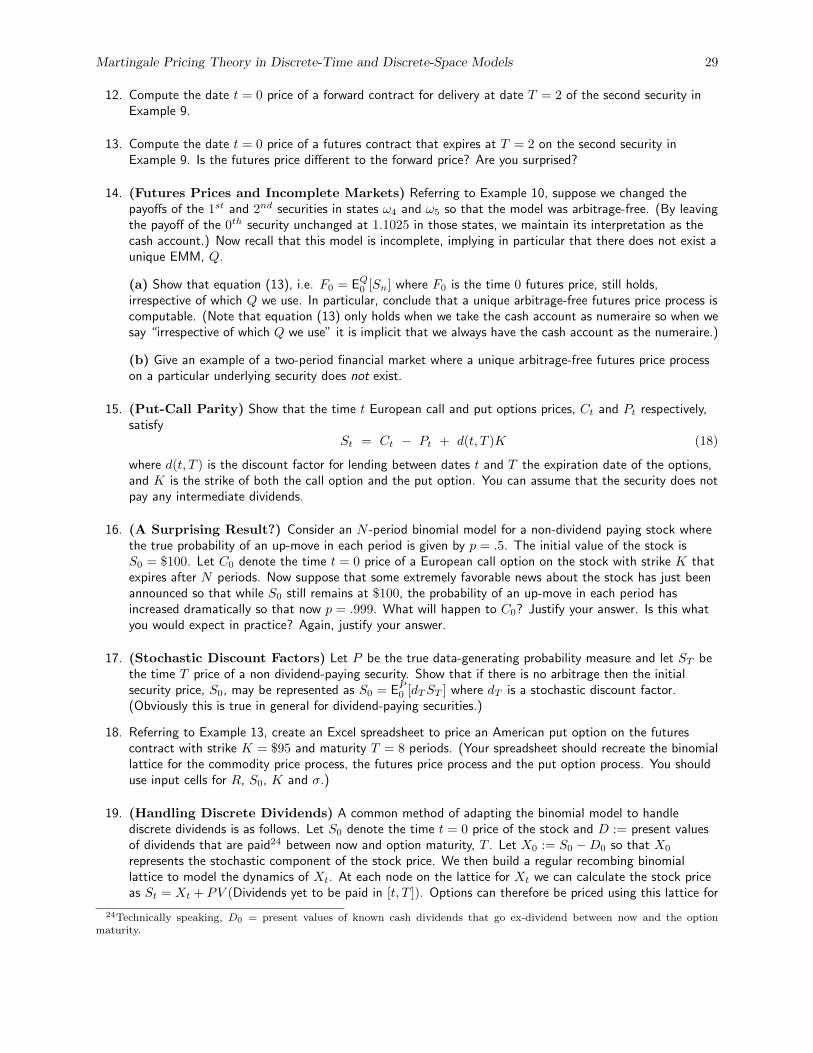
12. Compute the date t = 0 price of a forward contract for delivery at date T = 2 of the second security inExample 9.
13. Compute the date t = 0 price of a futures contract that expires at T = 2 on the second security inExample 9. Is the futures price different to the forward price? Are you surprised?
14. (Futures Prices and Incomplete Markets) Referring to Example 10, suppose we changed thepayoffs of the 1st and 2nd securities in states ω4 and ω5 so that the model was arbitrage-free. (By leavingthe payoff of the 0th security unchanged at 1.1025 in those states, we maintain its interpretation as thecash account.) Now recall that this model is incomplete, implying in particular that there does not exist aunique EMM, Q.
(a) Show that equation (13), i.e. F0 = EQ0 [Sn] where F0 is the time 0 futures price, still holds,irrespective of which Q we use. In particular, conclude that a unique arbitrage-free futures price process iscomputable. (Note that equation (13) only holds when we take the cash account as numeraire so when wesay “irrespective of which Q we use” it is implicit that we always have the cash account as the numeraire.)
(b) Give an example of a two-period financial market where a unique arbitrage-free futures price processon a particular underlying security does not exist.
15. (Put-Call Parity) Show that the time t European call and put options prices, Ct and Pt respectively,satisfy
St = Ct − Pt + d(t, T )K (18)
where d(t, T ) is the discount factor for lending between dates t and T the expiration date of the options,and K is the strike of both the call option and the put option. You can assume that the security does notpay any intermediate dividends.
16. (A Surprising Result?) Consider an N -period binomial model for a non-dividend paying stock wherethe true probability of an up-move in each period is given by p = .5. The initial value of the stock isS0 = $100. Let C0 denote the time t = 0 price of a European call option on the stock with strike K thatexpires after N periods. Now suppose that some extremely favorable news about the stock has just beenannounced so that while S0 still remains at $100, the probability of an up-move in each period hasincreased dramatically so that now p = .999. What will happen to C0? Justify your answer. Is this whatyou would expect in practice? Again, justify your answer.
17. (Stochastic Discount Factors) Let P be the true data-generating probability measure and let ST bethe time T price of a non dividend-paying security. Show that if there is no arbitrage then the initialsecurity price, S0, may be represented as S0 = EP0 [dTST ] where dT is a stochastic discount factor.(Obviously this is true in general for dividend-paying securities.)
18. Referring to Example 13, create an Excel spreadsheet to price an American put option on the futurescontract with strike K = $95 and maturity T = 8 periods. (Your spreadsheet should recreate the binomiallattice for the commodity price process, the futures price process and the put option process. You shoulduse input cells for R, S0, K and σ.)
19. (Handling Discrete Dividends) A common method of adapting the binomial model to handlediscrete dividends is as follows. Let S0 denote the time t = 0 price of the stock and D := present valuesof dividends that are paid24 between now and option maturity, T . Let X0 := S0 −D0 so that X0
represents the stochastic component of the stock price. We then build a regular recombing binomiallattice to model the dynamics of Xt. At each node on the lattice for Xt we can calculate the stock priceas St = Xt + PV (Dividends yet to be paid in [t, T ]). Options can therefore be priced using this lattice for
24Technically speaking, D0 = present values of known cash dividends that go ex-dividend between now and the optionmaturity.
Martingale Pricing Theory in Discrete-Time and Discrete-Space Models 30
Xt. (Note that the use of the closed interval [t, T ] rather than (t, T ] implicitly implies the option-holdergets the dividend if the option is exercised at time t and a dividend is paid at that date.)
Use this method to price a 6-month American call option on a stock with initial value S0 = 100, strikeK = 100 and a continuously compounded risk-free rate if r = 5%. You can assume σ = 30% for Xt andthat the stock pays a dividend of $5 in 4 months time. A 6-period lattice will suffice. Is the option pricethe same as the price of the corresponding European option? While this method of handling discretedividends is often used in practice, it does have some flaws. Can you identify any of them?
20. (A Foreign Currency EMM) Let Qf be an EMM for a foreign investor corresponding to some
foreign numeraire, Xf say. Note that Xft is then denominated in units of the foreign currency. Show that
Qf can also be used as an EMM for a domestic investor. What is the corresponding domestic numeraire?Is the converse also true, i.e., can any domestic EMM also be used as an EMM for a foreign investor?
21. (Martingale Pricing Theory and the CAPM) Is the Capital Asset Pricing Model (CAPM)consistent with martingale pricing theory? Justify your answer. (Recall that the CAPM is a one-periodmodel which states that the expected return, r̄ say, on any security satisfies r̄ = rf + β(r̄m − rf ) where rfis the risk-free rate, r̄m is the expected return on the market portfolio and β = Cov(r, rm)/Var(rm).)
22. (The Knapsack Problem: A Deterministic Dynamic Program) Assume that we have a vesselwhose maximum weight capacity is z and whose cargo is to consist of different quantities of N differentitems. Let vi denote the value of the ith type of item, wi the weight of the ith type of item, and xi thenumber of items of type i that are loaded in the vessel. The problem is to find the most valuable cargo,i.e., to maximize
∑Ni=1 xivi subject to the constraints
∑Ni=1 xiwi ≤ z and xi = 0, 1, 2, . . . Formulate this
problem as a dynamic programming problem.
23. (Dynamic Portfolio Optimization in Complete Markets) Referring to the model of Example 9,suppose you have a fixed initial wealth, W0 ≥ 0 at t = 0, and you wish to choose a trading strategy tomaximize P (W2 ≥ α) subject to P (W2 ≥ 0) = 1. (W2 is your date t = 2 wealth, α > 0 is a fixed
constant and to avoid a trivial solution you should assume S(n)0 EQ0 [α/S
(n)T ] > W0 where S
(n)i is the time i
price of the numeraire security.) Explain in detail how you would do this. Note also how your solution canbe adapted to handle the case where α is a stochastic benchmark. (Hint: You will need to solve adynamic program of the type given in Exercise 22 where each Xi is either 0 or 1. Why?)


![Option Pricing Under a Discrete-Time Markov Switching ... · arXiv:2006.15054v1 [q-fin.PR] 26 Jun 2020 Option Pricing Under a Discrete-Time Markov Switching Stochastic Volatility](https://img.dokumen.tips/doc/110x75/5fc5bcca12dd631bfe463aea/option-pricing-under-a-discrete-time-markov-switching-arxiv200615054v1-q-finpr.jpg)