Embed Size (px)
Citation preview
Chapter 4
Discrete-time Markov Chainsand Applications to PopulationGenetics
A stochastic process is a quantity that varies randomly from point to point of anindex set; for example, your total earnings after n plays of a game of chance, as afunction of the index n. Chapter 4 is about a class of stochastic processes calleddiscrete-time Markov chains and their application to population genetics. WhileChapter 3 was driven by the scientific questions of population genetics, Chapter 4is organized instead around its mathematical content. The reason for this changeof perspective is the incredible importance of Markov chains in scientific and en-gineering, whenever stochastic models are needed. In particular, they are appliedin many areas of quantitative biology beyond population genetics. This chapter ismeant to give the reader enough basic theory of Markov chains to understand theiruse in current biological literature, whatever the area. Nevertheless, in this chapterpopulation genetics will serve as the primary motivation and as the source of mostexamples.
To understand why stochastic processes are important in population genetics,think back to Chapter 3. All the models there impose the infinite population as-sumption: they set the frequency of a genotype, which is really random, equal tothe probability a mating produces that genotype, which is not. When this is done,genotype frequencies become deterministic functions of time, for which we were ableto derive difference equations.
However, when the population is small, fluctuations of genotype frequencies dueto chance cannot be ignored. For example, consider one locus with two alleles, Aand a, in a parent population for which fA = 0.9. Then, as we learned from Chapter3, the probability a random mating produces an AA offspring is f2
A = 0.81. If thenext generation consists of only 10 individuals produced by 10 independent ran-dom matings, the event all are AA has the small, but not insignificant, probability
1
2 CHAPTER 4. MARKOV CHAINS
(0.81)10 ≈ 0.107. So, allele a can disappear in the offspring population, not becauseit is less fit, but simply by chance, by what biologists call random genetic drift.Likewise, there is a chance that allele A could disappear. In fact, as we will seelater, when the alleles experience no mutation and the population maintains a con-stant size, one of the alleles will eventually disappear. This is completely differentfrom what happens in the infinite population model, for which fA is constant fromgeneration to generation. Thus, in small populations, randomness is so important afeature of the evolution of gene frequencies that they must be treated as stochasticprocesses.
The theory of Markov chains relies heavily on the use of conditional probabilitiesand conditional expectations. The reader may consult Sections 2.1.5 and 2.3.6 ofChapter 2 for the relevant background. This chapter will also make use of elementarylinear algebra.
4.1 Markov Chains: Introduction
4.1.1 Discrete-time, stochastic process models.
A discrete-time stochastic processes is a sequence of random variables, {X(0), X(1),X(2), . . .}, indexed by a discrete ‘time’ parameter t, t = 0, 1, 2, . . .. Whether ornot the index t represents time depends on the application, but the order of thesequence is important. Also, it is not essential that the first time be t = 0 or thattime increase by unit steps. These are just conventions that we use when discussingstochastic processes in general. Throughout the chapter, we denote a generic termof a stochastic process by X(t) and think of it as the random value of the processat time t. We denote the process itself by {X(t); t ≥ 0}, or, simply, {X(t)}.
In practice, X(t) will represent the ‘state’ of some system at time t. The setof all possible states is called the state space of the process, and we usually denoteit by E . For example, in population genetics models, X(t) may be the number ofindividuals with a certain genotype at time t. If the population maintains a constantsize N , the appropriate state space is E = {0, 1, . . . , N}. In later chapters, DNA istreated as a random sequence of bases X(1), X(2), . . . , X(T ); then X(t) representsthe base at site t along the DNA segment—hence t denotes a position rather thana time—and the state space is the DNA alphabet {A, T, C, G}. When E is finite, asin these examples, or countably infinite, we say E is discrete. This will be the casefor most models in this text.
Given a stochastic processes X = {X(t); t ≥ 0}, the expression,
P (X(0)=x0, X(1)=x1, . . . , X(t)=xt) , (4.1)
as a function of (x0, x1, . . . , xt), is the joint probability mass function of X(0), . . . , X(t),and is called a finite-dimensional distribution of {X(t); t ≥ 0}. It is often helpful tothink of P (X(0)=x0, X(1)=x1, . . . , X(t)=xt) as the probability that the process
4.1. MARKOV CHAINS: INTRODUCTION 3
follows the path, {X(0) = x0, X(1) = x1, . . . , X(t) = xt}, up to time t, and so wesometimes call it a path probability.
The collection of all finite dimensional distributions of a process determines howto compute the probability of any path, and thus provides a complete statisticaldescription of the process. A model of a stochastic process is therefore any set ofassumptions that determines, at least in principle, all its finite dimensional distri-butions. A model is allowed to contain unspecified parameters, in which case it issometimes called a parametric model.
To illustrate the terminology, let {X(0), X(1), . . .} represent a sequence of cointosses, with X(t) = 1, if toss t results in heads, and X(t) = 0, if tails. Theassumption, “X(0), X(1), · · · are independent tosses of a fair coin,” constitutes amodel, because it implies
P (X(0)=x0, X(1)=x1, . . . , X(t)=xt) = (1/2)t+1,
for any t and any sequence (x0, . . . , xt) of 0’s and 1’s, and hence it completely deter-mines all joint probabilities. The slightly more general assumption, “X(0), X(1), . . .are independent, identically distributed Bernoulli variables,” is a parametric modelin which the parameter is the unspecified probability, p := P(X(t)=1), because inthis case,
P (X(0)=x0, X(1)=x1, . . . , X(t)=xt) =t∏
i=0
P (X(i)=xi) = pn̂(1− p)t+1−n̂,
where n̂ =∑t
0 xi is the number of 1’s in the sequence (x0, . . . , xt). Hence, the finitedimensional distributions are all determined up to the unspecified value of p.
How does one model a stochastic process observed in nature? This requirestranslating assumptions about the physical causes of its behavior into conditionsdetermining its finite dimensional distributions. When the process evolves in time,it is often most natural to use conditional probabilities. For any time t ≥ 0,
P(X(0)=x0, . . . , X(t)=xt, X(t+1) = xt+1
)(4.2)
= P(X(t+1)=xt+1
∣∣∣X(0)=x0, . . . , X(t)=xt
)P(X(0)=x0, . . . , X(t)=xt
).
This is a consequence of the simple identity, P(A ∩ B) = P(A|B)P(B), when A ={X(t+1) = xt+1} and B = {X(0) = x0, . . . , X(t) = xt}. If t is thought of as thepresent time, the expression
P(X(t+1) = xt+1 | (X(0), . . . , X(t))=(x0, . . . , xt)
), t ≥ 0.
in (4.2) is a conditional probability for the value of the process one step aheadinto the future, given its entire past history; we call it a one-step-ahead conditionalprobability. As we see from equation (4.2), these conditional probabilities link the
4 CHAPTER 4. MARKOV CHAINS
joint distribution of (X(0), . . . , X(t), X(t+1)) to that of (X(0), . . . , X(t)), and thusthey determine how joint distributions evolve as time goes forward. Hence, we canmodel a stochastic process by specifying its one-step-ahead conditional probabilities.In practice, they can often be deduced directly from assumptions on the physicalnature of the process.
Example 4.1.1 Transitions between two states at random times.Imagine moving between two stations, labeled 0 and 1, and let X(t) denote
your station at time t. At each time, t, you flip a coin that lands heads up withprobability 0.25. If the flip comes up heads you move to the opposite station attime t+1; otherwise you stay put. All coin flips are independent. Then X(t) is astochastic process with state space {0, 1}.
Its one-step-ahead conditional probabilities are easy to calculate. Consider anyhistory, {X(0) = x0, X(1) = x1, . . . , X(t−1) = xt−1, X(t) = 0}, that ends up instation 0 at time t. Then, you will move to station 1 at the next time if your coinflip comes up heads. Since this flip is independent of all previous events and headshas probability 0.25,
P(
X(t+1)=1∣∣∣X(t)=0, X(t−1)=xt−1, . . . , X(0)=x0
)= P
(X(t+1)=1
∣∣∣X(t)=0)
= 0.25,
P(
X(t+1)=0∣∣∣X(t)=0, X(t−1)=xt−1, . . . , X(0)=x0
)= P
(X(t+1)=0
∣∣∣X(t)=0)
= 0.75.
Note that the past history, {X(t−1) = xt−1, . . . , X(0) = x0}, does not affect theseconditional probabilities. Only the fact that you are at station 0 at time t is relevant.The one-step ahead probabilities when X(t) = 1 are easily computed in the samemanner, and again they do not depend on what the process did before time t. �.
4.1.2 Markov Chains: Definition and basic properties
The one-step-ahead conditional probabilities in Example 4.1.1 depended on the pastonly through the given value X(t) = xt at the present time t. Markov chains aredefined by requiring this property to hold generally.
Definition. A stochastic process X = {X(t); t ≥ 0} taking values in (a discrete)state space E is called a Markov chain if
P(X(t+1) = xt+1 | X(0)=x0, . . . , X(t)=xt
)= P
(X(t+1) = xt+1 | X(t)=xt
)(4.3)
4.1. MARKOV CHAINS: INTRODUCTION 5
for every t ≥ 0 and for all sequences of states, x0, . . . , xt, for which both conditionalprobabilities are well-defined. (Both will be well-defined if and only ifP(X(0)=x0, . . . , X(t)=xt
)> 0.)
Markov chains are named in honor of the Russian mathematician, A. Markov(1856-1922), who did pioneering work in the definition and analysis of this class of pro-cesses.
We call (4.3) the Markov chain condition. The whole theory of Markov chainsflows out of this innocent-looking assumption. In particular, it implies a vastly moregeneral property called the Markov property, which says that at any time t, the pastand future of the process are conditionally independent, given the present. TheMarkov property is explained in Section 4.1.4.
Later in the text, we will also define continuous-time Markov chains. Until then,the term ‘Markov chain’ always means a discrete-time Markov chain.
If X is a Markov chain, P(X(t+1) = j | X(t) = i
)is called the probability of
transition from state i to state j at time t. If this probability does not depend on t,it is denoted by pij , and X is said to be time-homogeneous. The process of Example4.1.1 is clearly an example of a time-homogeneous Markov chain. Its state space isE = {0, 1}, and its transition probabilities are
p00 = 0.75, p01 = 0.25, p10 = 0.25, p11 = 0.75,
because the chain moves from the state it’s in to the other state if and only if thecoin toss results in heads, which has probability 0.25.
The default assumption in this chapter is that all Markov chains are time-homogeneous, and the term Markov chain should always be interpreted as time-homogeneous Markov chain.
Example 4.1.2. The two-state Markov chain. The general, two-state Markov chainis not much more complicated than Example 4.1.1. The two states can be almosteverything, but for convenience label them again as 0 and 1. A Markov chain movingbetween 0 and 1 is defined by four transition probabilities, p00, p01, p10, and p11.However, since 0 and 1 are the only states,
p00 + p01 = P(X(t+1)=0|X(t)=0) + P
(X(t+1)=1|X(t)=0)
= P(X(t+1) ∈ {0, 1}|X(t)=0) = 1.
Likewise, p10 + p11 = 1. Thus, the two transition probabilities, p01 and p10, com-pletely determine the two-state Markov chain. It is standard to denote p01 by λ andp10 by µ, so that
p00 = 1− λ, p01 = λ, p11 = µ and p10 = 1− µ.
6 CHAPTER 4. MARKOV CHAINS
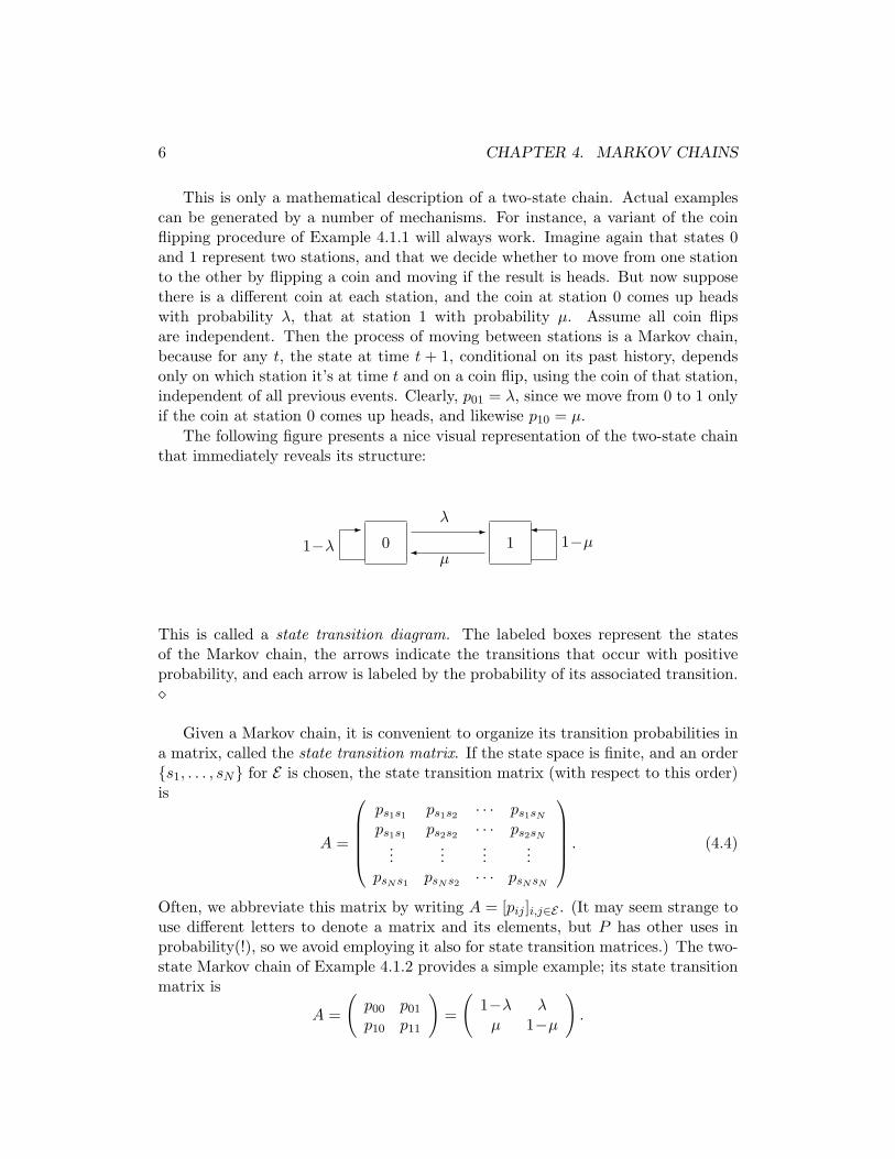
This is only a mathematical description of a two-state chain. Actual examplescan be generated by a number of mechanisms. For instance, a variant of the coinflipping procedure of Example 4.1.1 will always work. Imagine again that states 0and 1 represent two stations, and that we decide whether to move from one stationto the other by flipping a coin and moving if the result is heads. But now supposethere is a different coin at each station, and the coin at station 0 comes up headswith probability λ, that at station 1 with probability µ. Assume all coin flipsare independent. Then the process of moving between stations is a Markov chain,because for any t, the state at time t + 1, conditional on its past history, dependsonly on which station it’s at time t and on a coin flip, using the coin of that station,independent of all previous events. Clearly, p01 = λ, since we move from 0 to 1 onlyif the coin at station 0 comes up heads, and likewise p10 = µ.
The following figure presents a nice visual representation of the two-state chainthat immediately reveals its structure:
0 1-
λ
�µ
1−λ
-1−µ
�
This is called a state transition diagram. The labeled boxes represent the statesof the Markov chain, the arrows indicate the transitions that occur with positiveprobability, and each arrow is labeled by the probability of its associated transition.�
Given a Markov chain, it is convenient to organize its transition probabilities ina matrix, called the state transition matrix. If the state space is finite, and an order{s1, . . . , sN} for E is chosen, the state transition matrix (with respect to this order)is
A =
ps1s1 ps1s2 · · · ps1sN
ps1s1 ps2s2 · · · ps2sN
......
......
psNs1 psNs2 · · · psNsN
. (4.4)
Often, we abbreviate this matrix by writing A = [pij ]i,j∈E . (It may seem strange touse different letters to denote a matrix and its elements, but P has other uses inprobability(!), so we avoid employing it also for state transition matrices.) The two-state Markov chain of Example 4.1.2 provides a simple example; its state transitionmatrix is
A =
(p00 p01
p10 p11
)=
(1−λ λ
µ 1−µ
).
4.1. MARKOV CHAINS: INTRODUCTION 7
This can be read off directly from the state transition diagram.The row indexed by si in (4.4) is the vector of transition probabilities starting
from state si. Since the process must end up in some state, the sum of theseprobabilities over all states equals 1. That is,
N∑j=0
psisj =N∑
j=0
P(X(t+1)=sj |X(t)=si) = 1
for every row of A. Any square matrix of non-negative entries each of whose rowssums to 1 is called a stochastic matrix. Thus, state transition matrices are stochasticmatrices. Conversely, any stochastic matrix is a valid model for the transitionprobabilities of a Markov chain.
The next theorem is the main result of this section. It tells us how to computeany finite dimensional distribution of a Markov chain.
Theorem 1 Let {Xt; t ≥ 0} be a time-homogeneous Markov chain with transitionprobabilities {pij ; i, j ∈ E}. For any t ≥ 0 and any path {x0, . . . , xt},
P(X(0)=x0, X(1)=x1, . . . , X(t)=xt
)= P(X(0)=x0)px0x1px1x2 · · · pxt−1xt (4.5)
or, equivalently,
P(X(1)=x1, . . . , X(t)=xt
∣∣∣X(0)=x0
)= px0x1px1x2 · · · pxt−1xt (4.6)
Conversely, if either of these is always true, {X(t); t ≥ 0} is a Markov chainwith transition probabilities {pij ; i, j ∈ E}.
Formula (4.5) is easy to remember. Think of a path (x0, x1, . . . , xt) as an initialstate x0 followed by a series of transitions x0 → x1 → x2 → · · · → xt; the probabilitya Markov chain follows this path is the probability that it starts at x0, times theproduct of the transition probabilities between successive states along the path.
The probability mass function,
P(X(0) = x), x ∈ E ,
is called the initial (probability) law of {X(t); t ≥ 0}, because it is the law of X(0)at the initial time t = 0. Theorem 1 implies that an initial law and a state transitionmatrix completely determine a model of a Markov chain, because, by equation (4.5),they specify all finite dimensional distributions. In practice the initial law is oftenincidental, and then we regard the state transition matrix alone as a model, onewhich allows arbitrary initial laws.
Proof of Theorem 1. The proof of (4.5) is by iterated conditioning. For convenience,denote P
(X(0)=x0, X(1)=x1, . . . , X(t)=xt) by Pt(x0, x1, . . . , xt). By conditioning
8 CHAPTER 4. MARKOV CHAINS
on the event {X(0) = x0, . . . , X(t − 1) = xt−1} using (4.2), and then applying theMarkov condition,
Pt(x0, . . . , xt−1, xt) = P(X(0)=x0, X(1)=x1, . . . , X(t−1)=xt−1
)× P
(X(t)=xt
∣∣∣ X(0)=x0, . . . , X(t−1)=xt−1
)= Pt−1(x0, . . . , , xt−1)pxt−1xt (4.7)
The parameter t ≥ 1 in this argument is arbitrary, and if we apply it with t replacedby t − 1, Pt−1(x0, . . . , xt−1, xt−1) = Pt−2(x0, . . . , xt−2)pxt−2xt−1 . Substituting backinto (4.7),
Pt(x0, . . . , xt) = Pt−2(x0, . . . , xt−2)pxt−2xt−1pxt−1xt .
By continuing this procedure backwards in time, we arrive finally at (4.5).
Equation (4.6) is just the same as (4.5) if both sides of (4.5) are divided byP(X(0)=x0). Conversely if (4.5) is true,
P(X(t+1)=xt+1
∣∣∣X(0)=x0, . . . , X(t)=xt
)=
P(X(0)=x0, . . . , X(t)=xt, X(t+1)=xt+1
)P(X(0)=x0, . . . , X(t)=xt
)=
P(X(0)=x(0))px0x1 · · · pxt−1xtpxtxt+1
P(X(0)=x(0))px0x1 · · · pxt−1xt
= pxtxt+1 ,
which proves the Markov condition. �
Example 4.1.3. Consider the two state Markov chain of Example 4.1.2 and supposeat time t = 0, it is equally likely to be in either of the two states, i.e., ρ0(0) =ρ1(0) = 1/2. Then
P((X(0), . . . , X(5))=(1, 1, 0, 0, 0, 1)
)= ρ1(0)p11p10p00p00p01
= (1/2)(1−µ)µ(1− λ)2λ. �
4.1. MARKOV CHAINS: INTRODUCTION 9
4.1.3 More Examples.
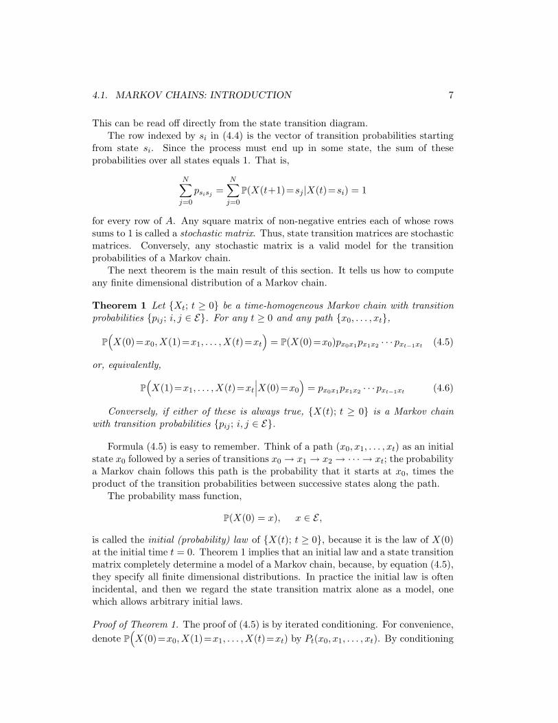
Example 4.1.4. Simple random walk. Simple random walk is the integer-valuedMarkov chain defined by the state transition diagram:
· · · −1 0 1 2-p
�q
-p
�q
-p
�q
-p
�q
-p
�q
· · ·
Equivalently, if i and j are any integers,
pij =
p, if j = i+1;q, if j = i−1;0, if |j − i| > 1.
(4.8)
Here, 0 < p < 1 and p + q = 1. Thus, the simple random walk moves frominteger to integer by unit steps only, at each time taking one step to the right withprobability p and one step to the left with probability q = 1 − p, independently ofits present position and past history. When p = q = 1/2, simple random walk iscalled symmetric, simple random walk.
There is an easy way to construct a simple random walk. Let X(0) denotea random, integer-valued, initial position. Assume that ξ1, ξ2, . . . are independentrandom variables, independent of X(0), and all having the distribution,
P (ξt =1) = p and P (ξt =−1) = 1− p = q.
Then X(t) = X(0) +∑
i=1 ξi, t ≥ 0, defines a simple random walk with transitionprobabilities as in (4.8). This is easy to see. For each t, X(t) −X(t−1) = ξt, andthus the ξt represents the tth step the process takes. Suppose X(t) = i is given.Since the (t + 1)st step, ξt+1, is independent of all other steps and of X(0), it clearthat X(t+1) = X(t) + ξt+1 = i + ξt+1 does not depend on the history of theprocess before time t, and so {X(t)} is a Markov chain. It has the correct transitionprobabilities because pi,i+1 = P(X(t+1) = i+1|X(t) = i) = P(ξt+1 = 1) = p andpi,i−1 = P(X(t+1)= i−1|X(t)= i) = P(ξt+1 =−1) = q.
Simple random walk is sometimes described picturesquely as the ‘drunkard’swalk.’ A drunk walks out of a bar—no, this is not the start of a joke!—and staggersup and down the street, taking unit-sized steps. The poor fellow is so inebriatedthat each new step is independent of all his previous efforts. If all steps have thesame probability of moving him up or down the street, he performs a simple randomwalk.
There is also a gambling interpretation. Imagine successive, independent plays,on each of which you win a dollar with probability p and lose a dollar with probabilityq. If ξt represents what you win on play t, then X(t) = X(0) +
∑t1 ξi is your total
fortune after t plays, when X(0) is the amount of money you start with.
10 CHAPTER 4. MARKOV CHAINS
The adjective ‘simple’ in ‘simple random walk’ means that the process moves byinteger steps only. The term, ‘random walk’, is also used for any process of the form
Y (t) = Y (0) +t∑1
ηi,
where Y (0) is a random variable, and η1, η2, . . . are independent, identically dis-tributed random variables, which are also independent of Y (0). See Exercise 4.10for an example. �
Example 4.1.5. The Wright-Fisher model for genotype evolution in a finite popula-tion: selectively neutral, one locus case.
Study this example closely! It is the basic stochastic model of population ge-netics. It is named after R.A. Fisher (1890-1962), a British statistician, and SewallWright (1889-1988), an American geneticist, who made pioneering contributions tothe discipline.
Let A be an allele, and let X(t) denote the number of A’s in the allele pool ofgeneration t, in a finite population. The selectively neutral, Wright-Fisher model isa model for how X(t) evolves randomly. It assumes: (i) the species is monecious anddiploid, and the size of the population remains constant; (ii) generations are non-overlapping; (iii) each generation is produced from the previous one by independentrandom matings; (iv) there is no selection, mutation, or migration. Compare thesehypotheses to the infinite population model defined in Section 3.3.1. The onlydifferences are that the population is finite in size and that random matings areexplicitly assumed to be independent. It is not important to the model how manyother alleles there are at the locus of A.
We will show how assumptions (i)—(iv) translate directly into a Markov chainmodel for {X(t)}. Of course, X(t) is always a non-negative integer, and if N denotesthe (constant) size of the population, it can be no larger than 2N . Thus, the statespace for the process E = {0, 1, . . . , 2N}.
Now, let t be any time, and fix a past history, {X(0) = i0, . . . , X(t− 1) =it−1, X(t) = i}, ending up with i alleles of type A in generation t. We want tocompute the conditional distribution of X(t+1). By assumptions (i) and (iii),generation t+1 is created by N , independent, random matings of generation tparents. From Chapter 3, the genotype produced by a random mating is the resultof two independent, random samples of the allele pool of generation t. Thus, theallele pool of generation t + 1 is created by 2N independent random samples. Now,the probability of randomly selecting A from the allele pool of generation t is itsfrequency, and since X(t) = i is given, this frequency is i
2N . Recall that the numberof successes in n independent trials, when p is the probability of success, has thebinomial distribution with parameters n and p. Counting the selection of A as asuccess, it follows that, given X(0) = i0, . . . , X(t−1) = it−1, and X(t) = i,
X(t+1) is binomial with parameters n = 2N and p = i/2N .
4.1. MARKOV CHAINS: INTRODUCTION 11
This has two consequences. First, this distribution depends only on X(t) = i, noton the values of X(s) for times s strictly prior to t, and therefore {X(t)} does indeedsatisfy the Markov condition. Second, it tells that that the transitions probabilitiesare given by the binomial distribution:
pij = P(
X(t+1) = j∣∣∣X(t)= i
)=
(2N
j
)(i
2N
)j (1− i
2N
)2N−j
, 0 ≤ i, j ≤ 2N.
(4.9)Two states deserve special attention, states 0 and 2N . State 0 means there are
no alleles A, and if this is the case, they will never appear in future generations, sincethere is no mutation in this model. Thus p00 = 1 and p0j = 0 for all 1 ≤ j ≤ 2N .Likewise, p2N,2N = 1, because once the chain enters state 2N , no a alleles are leftand it must stay in state 2N ever after.
In general, a state i of a Markov chain is said to be absorbing if pii = 1, becauseonce the chain hits state i, it remains there forever. Thus, states 0 and 2N of theWright-Fisher chain are absorbing.
When 0 < i < 2N , the formula of (4.9) shows that pij > 0 for any other state j,and so the chain can move from i to any other state j in one step. Thus states 0 and2N are the only absorbing states. It is of little use to write down a state transitiondiagram for a Wright-Fisher chain, even for fairly small values of N . The diagramwill be crowded with arrows going from each non-absorbing state to all others andwill not help us understand the chain better.
Let
Y (t) =X(t)2N
.
Y (t) is the frequency of allele t in generation t and it, rather than X(t), is the actualobject of interest. {Y (t)} is also called the Wright-Fisher process and is really theone we should work with. We have defined the equivalent process, {X(t)}, fornotational convenience. It is much cleaner to write the transition probability pij
for the transition of X(t) from i to j, then the corresponding transition probability,pi/2N,j/2N , for Y (t)! And as long as N is fixed, it makes no difference whether weanalyze {X(t)} or {Y (t)}. However, when we wish to compare the Wright-Fisherchain for different values of N , it is much better to use {Y (t)}, because it representsa frequency no matter what N is.
Example 4.1.6. The Moran model. This is named in honor of the Australian ap-plied probabilist P.A.P. Moran (1917-1988). It is a finite population model withoverlapping generations, but without selection, mutation or migration. However, itassumes that reproduction is asexual, by simple duplication. The model treats apopulation divided into two types, which shall be denoted by the letters A and a.One might think of these letters as denoting genotypes or alleles, but that is notnecessary, and a may just represent ‘not A.’
12 CHAPTER 4. MARKOV CHAINS
The population changes according to the following mechanism. At each timet, two individuals are selected from the current population by independent randomsampling with replacement. The first individual gives birth to a copy of itself, whichjoins the population together with its parent. The second individual is removedfrom the population (it dies). The result of these two steps is the population attime t+1. The random samplings at different times are all independent.
Note the following features of this model. First, since one individual is addedand one removed at each stage, the population remains constant in size. Second,the choice of who reproduces and who dies is made with replacement, and so theindividual chosen to reproduce may be the same as the one chosen to die, with theend result that it is just replaced with a copy of itself. Finally, there is no selectionin the model, because in every generation each individual has the same chance toreproduce or die, irrespective of type.
Let X(t) denote the number of individuals of type A at stage t, and let N denotethe total size of the population. We will argue that X = {X(t)}t≥0 is a Markovchain and calculate its transition probabilities.
Suppose X(t) = i and 0 < i < N , and perform the random selection, copy andreplacement experiment described above. The probability of selecting type A is theni/N and of selecting a is (N − i)/N in each of the two samples. There are threepossibilities. The first is that a type A is chosen to reproduce and a type a to die.
This happens with probabilityi
N
(N−i)N
and increases the number of A’s by one.Thus,
P(X(t+1)= i+1
∣∣∣ X(t)= i)
=i(N−i)
N2.
The second possibility is that the opposite occurs, a type a is chosen to reproduceand a type A to die, in which case X(t+1) = i− 1. Again,
P(X(t+1)= i−1
∣∣∣X(t)= i)
=i(N−i)
N2.
Finally, if both individuals selected are the same type, the overall number of typeA’s remains unchanged. As this is the only remaining case,
P(X(t+1)= i
∣∣∣X(t)= i)
= 1− 2i(N−i)
N2.
This can also be expressed as the sum of the probability of choosing A twice andthe probability of choosing a twice:
P(X(t+1)= i
∣∣∣X(t)= i)
=(
i
N
)2
+(
N − i
N
)2
=i2 + (N − i)2
N2.
Since these are the only possibilities, pij = 0 if |j − i| > 1.If i = 0, there are no type A’s, and since no mutation occurs, type A’s cannot
enter the population at the next, or at any future, time. Thus, p00 = 1 and 0 is
4.1. MARKOV CHAINS: INTRODUCTION 13
absorbing. Similarly, if i = N , type a’s can never enter the population and N isabsorbing.
This entire analysis is unchanged if values of X(s) at times s previous to t arealso given—only X(t) = i is relevant. Thus X satisfies the Markov chain condition,and so it is a Markov chain.
As an example, we write down the state transition matrix for N = 4 when thestates are in the order 0, 1, 2, 3, 4; the reader may easily verify the values of theentries:
1 0 0 0 0316
1016
316 0 0
0 14
12
14 0
0 0 316
1016
316
0 0 0 0 1
�
Example 4.1.7. Birth-and-death chains. These are a class of Markov chains gener-alizing random walk. The Moran model is a particular example.
Let E be a set of consecutive integers; E could be finite or infinite. A birth-and-death chain on E is a Markov chain which only makes transitions of at most unit size,but which allows the transition probabilities to depend on the present state. Thus,for each i ∈ E , there are non-negative numbers, pi, qi, and ri, with pi + qi + ri = 1,such that
pij =
pi, if j = i+1 and i+1 ∈ E ;ri, if j = i;qi, if j = i−1, and i−1 ∈ E ;0, otherwise.
Because of this structure, the state transition matrix of a birth-and-death chainhas a characteristic form; its only non-zero entries are along, above, and below thediagonal. For example, the state transition matrix of the general birth-and-deathchain on {0, 1, . . . , N} is
A =
1−p0 p0 0 0 · · · · · · 0q1 r1 p1 0 · · · · · · 00 q2 r2 p2 · · · · · · 0...
......
...0 · · · · · · · · · qN−1 rN−1 pN−1
0 · · · · · · · · · 0 qN 1− qN
. �
In all examples so far, the Markovian nature of each process was fairly obviousfrom its definition. Sometimes, the process of direct interest is not Markovian. When
14 CHAPTER 4. MARKOV CHAINS
this happens, it is often possible to embed it in a Markov process by expanding thestate space, and this may be helpful in analyzing the model. The next exampleillustrates this point.
Example 4.1.8. Modeling DNA. Take a sample of DNA and let X(1), X(2), . . . , X(K)represent the successive bases along one of its strands, read in the 5′ to 3′ direction.This will be a string of letters from the DNA alphabet, {A, T, C, G}.
We are interested in stochastic models for X(1), . . . , X(K). This may seem odd.What is random about a string of DNA? After all, it just is what it is. However,many experiments involve sampling DNA from a population. Since DNA sequencesvary from member to member, the sampled sequence is effectively random. In fact,the probability distribution of this random sample is precisely the object of interestin studies of the variation DNA sequences across a population.
Markov chain models of DNA sequences are often used, and we will discusssome later in the text. But how reasonable are they? The Markov condition wouldrequire that the conditional distribution of the base X(t+1) at position t + 1, giventhe bases X(1), . . . , X(t), depends only on the base X(t) at position t. This seemsunlikely a priori, especially for DNA in coding regions. DNA codons are threebase pairs long and the sequence in which they occur codes for proteins. Thus, forexample, one might expect that the conditional distribution of X(t+1) given say,X(t−1) = A,X(t) = A could be different than the conditional distribution givenX(t−1) = C,X(t) = A. A better model for DNA might be to assume that {X(t)}is a k-Markov chain, for some k > 1. This means that, for any t, k previous basesalways suffice to characterize a one-step-ahead conditional probability: that is,
P(X(t+1) = xt+1 | X(0)=x0, . . . , X(t)=xt
)= P
(X(t+1) = xt+1 | X(t)=xt, . . . , X(t−k+1) = xt−k+1
). (4.10)
(For this to make sense, t ≥ k − 1.)k-Markov chains can be analyzed on their own terms, but it is just as easy to
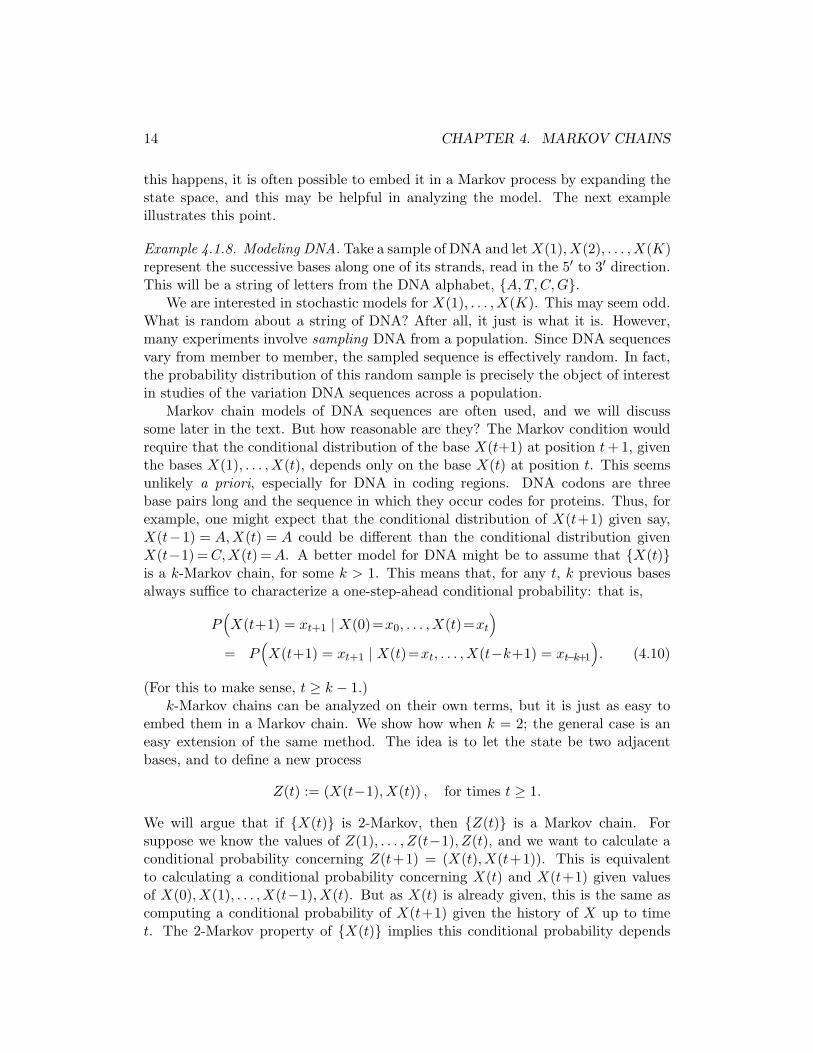
embed them in a Markov chain. We show how when k = 2; the general case is aneasy extension of the same method. The idea is to let the state be two adjacentbases, and to define a new process
Z(t) := (X(t−1), X(t)) , for times t ≥ 1.
We will argue that if {X(t)} is 2-Markov, then {Z(t)} is a Markov chain. Forsuppose we know the values of Z(1), . . . , Z(t−1), Z(t), and we want to calculate aconditional probability concerning Z(t+1) = (X(t), X(t+1)). This is equivalentto calculating a conditional probability concerning X(t) and X(t+1) given valuesof X(0), X(1), . . . , X(t−1), X(t). But as X(t) is already given, this is the same ascomputing a conditional probability of X(t+1) given the history of X up to timet. The 2-Markov property of {X(t)} implies this conditional probability depends
4.1. MARKOV CHAINS: INTRODUCTION 15
only on the values of X(t−1) and X(t), and hence only on the value of Z(t) =(X(t−1), X(t)), irrespective of the values of Z(s) for s ≤ t−1. This is the Markovchain condition for {Z(t); t ≥ 1}, as we wanted to show. (See Exercise 4.1.9 for therudiments of a direct analysis of 2-Markov chains.)
Of course, whether a k-Markov chain for k > 1 is a better model for DNA thana Markov chain is a question to be resolved by fitting alternative models to dataand seeing which works best. The purpose of this example was to emphasize themeaning and scope of the Markov condition, (4.3), and how its use might guide thecorrect choice of a state space. �
4.1.4 The Markov property.
According to the Markov condition, (4.3), each new state of a Markov chain isdetermined randomly by a mechanism depending only on the current state andotherwise independent of the previous history of the chain. We can imagine thereis a separate machine for each state. When the chain gets to state i, we push thebutton on its machine, which returns a random state j to move to next, where theprobability of j is pij for all states j. (For instance, the ‘machine’ we used for two-state chains was coin flipping.) The intuitive consequences of this picture go beyondone-step-ahead conditional probabilities. For example, it ought to be true that
P(X(t+1)=xt+1 | X(t−1)=xt−1, X(t)=xt
)= P
(X(t+1)=xt+1 | X(t)=xt
)(4.11)
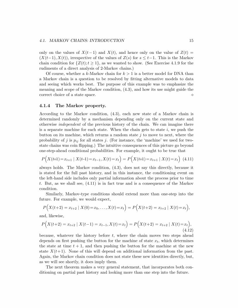
always holds. The Markov condition, (4.3), does not say this directly, because itis stated for the full past history, and in this instance, the conditioning event onthe left-hand side includes only partial information about the process prior to timet. But, as we shall see, (4.11) is in fact true and is a consequence of the Markovcondition.
Similarly, Markov-type conditions should extend more than one-step into thefuture. For example, we would expect,
P(X(t+2) = xt+2 | X(0)=x0, . . . , X(t)=xt
)= P
(X(t+2) = xt+2 | X(t)=xt
),
and, likewise,
P(X(t+2) = xt+2 | X(t−1) = xt−1, X(t)=xt
)= P
(X(t+2) = xt+2 | X(t)=xt
),
(4.12)because, whatever the history before t, where the chain moves two steps aheaddepends on first pushing the button for the machine of state xt, which determinesthe state at time t + 1, and then pushing the button for the machine at the newstate X(t+1). None of this will depend on additional information from the past.Again, the Markov chain condition does not state these new identities directly, but,as we will see shortly, it does imply them.
The next theorem makes a very general statement, that incorporates both con-ditioning on partial past history and looking more than one step into the future.
16 CHAPTER 4. MARKOV CHAINS
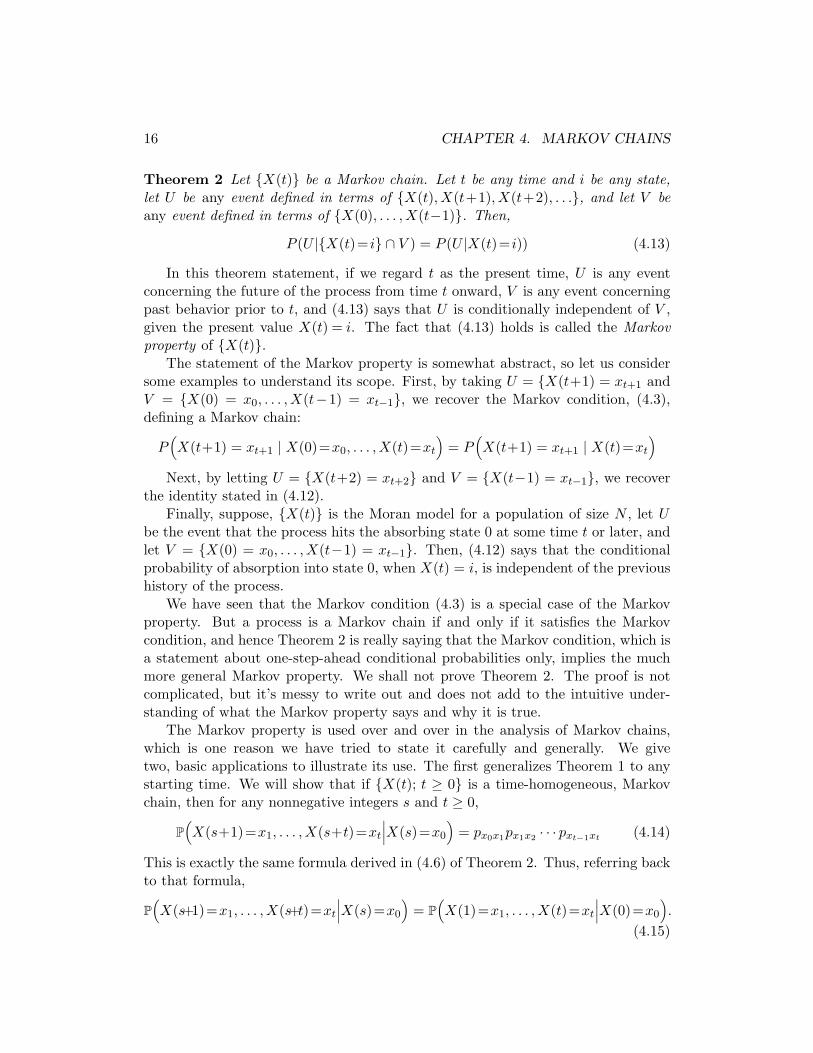
Theorem 2 Let {X(t)} be a Markov chain. Let t be any time and i be any state,let U be any event defined in terms of {X(t), X(t+1), X(t+2), . . .}, and let V beany event defined in terms of {X(0), . . . , X(t−1)}. Then,
P (U |{X(t)= i} ∩ V ) = P (U |X(t)= i)) (4.13)
In this theorem statement, if we regard t as the present time, U is any eventconcerning the future of the process from time t onward, V is any event concerningpast behavior prior to t, and (4.13) says that U is conditionally independent of V ,given the present value X(t) = i. The fact that (4.13) holds is called the Markovproperty of {X(t)}.
The statement of the Markov property is somewhat abstract, so let us considersome examples to understand its scope. First, by taking U = {X(t+1) = xt+1 andV = {X(0) = x0, . . . , X(t−1) = xt−1}, we recover the Markov condition, (4.3),defining a Markov chain:
P(X(t+1) = xt+1 | X(0)=x0, . . . , X(t)=xt
)= P
(X(t+1) = xt+1 | X(t)=xt
)Next, by letting U = {X(t+2) = xt+2} and V = {X(t−1) = xt−1}, we recover
the identity stated in (4.12).Finally, suppose, {X(t)} is the Moran model for a population of size N , let U
be the event that the process hits the absorbing state 0 at some time t or later, andlet V = {X(0) = x0, . . . , X(t−1) = xt−1}. Then, (4.12) says that the conditionalprobability of absorption into state 0, when X(t) = i, is independent of the previoushistory of the process.
We have seen that the Markov condition (4.3) is a special case of the Markovproperty. But a process is a Markov chain if and only if it satisfies the Markovcondition, and hence Theorem 2 is really saying that the Markov condition, which isa statement about one-step-ahead conditional probabilities only, implies the muchmore general Markov property. We shall not prove Theorem 2. The proof is notcomplicated, but it’s messy to write out and does not add to the intuitive under-standing of what the Markov property says and why it is true.
The Markov property is used over and over in the analysis of Markov chains,which is one reason we have tried to state it carefully and generally. We givetwo, basic applications to illustrate its use. The first generalizes Theorem 1 to anystarting time. We will show that if {X(t); t ≥ 0} is a time-homogeneous, Markovchain, then for any nonnegative integers s and t ≥ 0,
P(X(s+1)=x1, . . . , X(s+t)=xt
∣∣∣X(s)=x0
)= px0x1px1x2 · · · pxt−1xt (4.14)
This is exactly the same formula derived in (4.6) of Theorem 2. Thus, referring backto that formula,
P(X(s+1)=x1, . . . , X(s+t)=xt
∣∣∣X(s)=x0
)= P
(X(1)=x1, . . . , X(t)=xt
∣∣∣X(0)=x0
).
(4.15)
4.1. MARKOV CHAINS: INTRODUCTION 17
This is a natural expression of the time-homogeneity of the process. It says that theprocess starting from i at time s behaves the same as the process starting from i attime 0.
To derive (4.14), we shall use the general identity:
P(A ∩B|C) = P(A|B ∩ C)P(B|C)
Taking A = {X(s+ t) = xt}, B = {X(s+1) = x1, . . . , X(s+ t−1) = xt−1}, andC = {X(s) = x0}, we get
P(X(s+1)=x1, . . . , X(s+t)=xt
∣∣∣X(s)=x0
)= P
(X(s+t)=xt
∣∣∣X(s)=x0, X(s+1)=x1, . . . , X(s+t−1)=xt−1)
× P(X(s+1)=x1, . . . , X(s+t−1)=xt−1
∣∣∣X(s)=x0
).
But by the Markov property, the first term on the right-hand side is simply thetransition probability pxt−1xt , and thus, reversing the order of the product,
P(X(s+1)=x1, . . . , X(s+t)=xt
∣∣∣X(s)=x0
)= P
(X(s+1)=x1, . . . , X(s+t−1)=xt−1
∣∣∣X(s)=x0
)· pxt−1xt .
Now apply the same method again to the first term on the right-hand side: then,
P(X(s+1)=x1, . . . , X(s+t)=xt
∣∣∣X(s)=x0
)= P
(X(s+1)=x1, . . . , X(s+t−2)=xt−2
∣∣∣X(s)=x0
)· pxt−2xt−1pxt−1xt .
Continuing in this fashion will eventually bring you to equation (4.14).
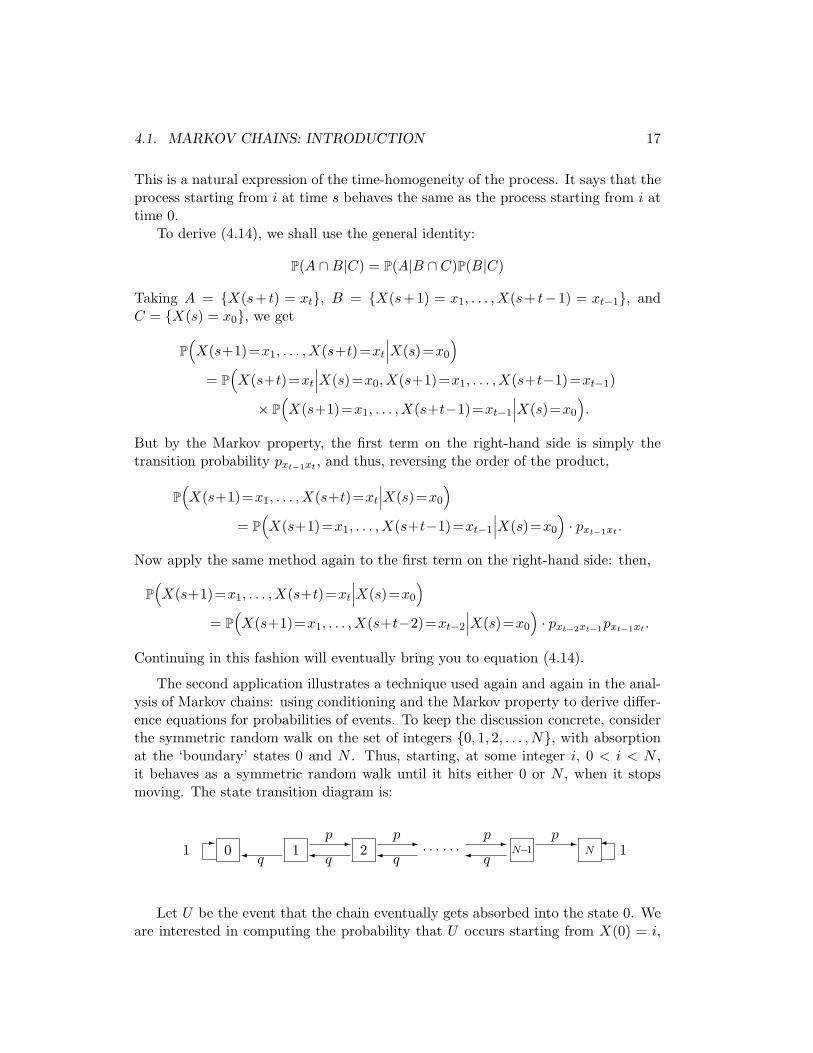
The second application illustrates a technique used again and again in the anal-ysis of Markov chains: using conditioning and the Markov property to derive differ-ence equations for probabilities of events. To keep the discussion concrete, considerthe symmetric random walk on the set of integers {0, 1, 2, . . . , N}, with absorptionat the ‘boundary’ states 0 and N . Thus, starting, at some integer i, 0 < i < N ,it behaves as a symmetric random walk until it hits either 0 or N , when it stopsmoving. The state transition diagram is:
01-
1 2 · · · · · · N−1�q
-p�
q
-p�
q
-p�
q
-pN 1
�
Let U be the event that the chain eventually gets absorbed into the state 0. Weare interested in computing the probability that U occurs starting from X(0) = i,
18 CHAPTER 4. MARKOV CHAINS
0 ≤ i ≤ N . This is called the gambler’s ruin problem, the idea being that X(t) isthe fortune after t plays of a game of chance in which the gambler wins a dollarwith probability p and loses with probability q. N is the total amount of money atstake between him and the casino and i is the amount he starts with. He will playeither until he wins all N and breaks the bank, or he goes broke (ruin). What isthe probability of ruin?
To answer this question, we will let gi = P(U |X(0) = i) and derive a differenceequation for gi, 0 ≤ i ≤ N . First note that, by definition,
g0 = 1 and gN = 0 (4.16)
Now suppose X(0) = i, where 0 < i < N . The central idea is to condition on wherethe chain moves next. There only two possibilities: it moves to i+1, which happenswith probability p, or to i − 1, which happens with probability q. By the rule oftotal probabilities,
gi = P(U |X(0)= i,X(1)= i + 1
)· p + P
(U |X(0)= i,X(1)= i− 1
)· q. (4.17)
Now U occurs if and only if the sequence {X(1), X(2), . . .} hits 0 before N . Thus,by the Markov property,
P(U |X(0)= i,X(1)= i + 1
)= P
({X(1), X(2), . . .} hits 0 before N
∣∣∣X(0)= i,X(1)= i + 1)
= P({X(1), X(2), . . .} hits 0 before N
∣∣∣X(1)= i + 1)
This last expression is the probability of ruin starting in state i + 1 at time s = 1.But, as just observed, a time-homogeneous chain starting in a state x at time sbehaves just like the chain starting at x at time 0. Thus, the probability of ruinstarting in state i + 1 at time s = 1 is the same is the same as the probability ofruin starting in state i + 1 at time s = 0, and this is, by definition, gi+1. By similarreasoning,
P(U |X(0)= i,X(1)= i− 1
)= gi−1.
Using these results in equation (4.17), we arrive at the difference equation,
gi = pgi+1 + qgi−1, 0 < i < n. (4.18)
To find gi for all i, we need to solve this equation with the ‘boundary’ conditions in(4.16). The solution, which you are asked to verify in Exercise 4.1.11, is:
gi =1− (q/p)i
1− (q/p)N, if p 6= q, gi =
i
N, if p = q = 1
2 . (4.19)
Later, we will solve similar problems for the Moran and Wright-Fisher chains usinga different method.
4.1. MARKOV CHAINS: INTRODUCTION 19
4.1.5 Exercises
4.1.1. Consider a three state Markov chain with transition probability matrix:
0 1 2
0 1/4 1/4 1/21 1/2 1/4 1/42 1/4 1/2 1/4
a) Write down a state transition diagram for this chain.b) Suppose P(X(0) = 1) = 1. Find the probability that P(X(2) = 0) by adding the
probabilities of all paths that lead from state 1 to state 0 in two steps.
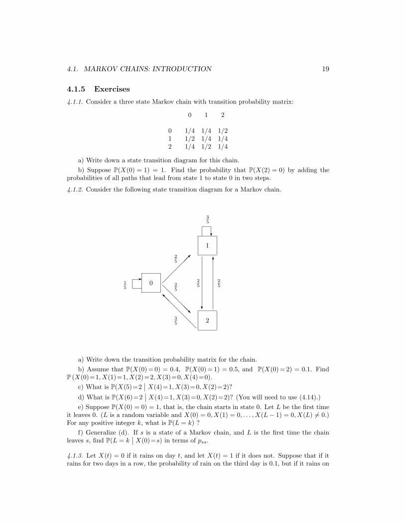
4.1.2. Consider the following state transition diagram for a Markov chain.
0
1
2
��
����
25
?
6
@@
@@@R
25
@@
@@
@@I
35
15
-
?
25
25
35
a) Write down the transition probability matrix for the chain.b) Assume that P(X(0) = 0) = 0.4, P(X(0) = 1) = 0.5, and P(X(0) = 2) = 0.1. Find
P (X(0)=1, X(1)=1, X(2)=2, X(3)=0, X(4)=0).c) What is P(X(5)=2
∣∣ X(4)=1, X(3)=0, X(2)=2)?
d) What is P(X(6)=2∣∣ X(4)=1, X(3)=0, X(2)=2)? (You will need to use (4.14).)
e) Suppose P(X(0) = 0) = 1, that is, the chain starts in state 0. Let L be the first timeit leaves 0. (L is a random variable and X(0) = 0, X(1) = 0, . . . , X(L− 1) = 0, X(L) 6= 0.)For any positive integer k, what is P(L = k) ?
f) Generalize (d). If s is a state of a Markov chain, and L is the first time the chainleaves s, find P(L = k
∣∣ X(0)=s) in terms of pss.
4.1.3. Let X(t) = 0 if it rains on day t, and let X(t) = 1 if it does not. Suppose that if itrains for two days in a row, the probability of rain on the third day is 0.1, but if it rains on
20 CHAPTER 4. MARKOV CHAINS
only one of two successive days, the probability of rain on the third is 0.2, and if it is sunnyfor two days in a row, the probability of rain on the third day is 0.3.
a) Explain why {X(t); t ≥ 0} is not a Markov chain, but is a 2-Markov chain.b) Let Z(t) = (X(t − 1), X(t)). As explained in the text, this will be a Markov chain.
List its states and calculate its state transition matrix.
4.1.4. (a) Consider the Wright-Fisher chain with N = 10. Suppose P (X(0)=5) = 1. FindP (X(2)=10). (Follow the procedure of Exercise 4.1.1.)
(b) For the Moran model with N = 4 and P(X(0)=1) = 1, calculate P(X(3)=0) andP(X(3)=1).
4.1.5. In this problem, we consider a process in the spirit of the Moran chain, but it is nota model of reproduction. Let X(n) denote the number of black marbles at time t in anurn containing 100 black and white marbles. The number of black marbles X(t+1) will bedetermined by the following experiment. Draw two marbles at random (random selectionwithout replacement). If two black marbles are drawn, return a black and white marble tothe urn (you have a collection of spare black and white marbles to use). If a white and ablack are drawn, simply return them to the urn. If two white marbles are drawn, return awhite and a black to the urn. The experiments producing X(n + 1) from X(n) for differentn are independent. Show that {X(t)} is a birth and death chain and compute its transitionprobabilities. Does this chain have absorbing states?
4.1.6. (Moran model with mutation). Suppose that in the Moran model, if a type A ischosen to reproduce its offspring mutates from A to a with probability u, and if a type areproduces its offspring mutates to type A with probability v. Show that the transitionprobabilities are
pi,i+1 =i(N − i)
N2(1− u) +
(N − i)2
N2· v
pi,i−1 =i(N − i)
N2(1− v) +
i2
N2· u
pii =i(N − i)
N2(u + v) +
(N − i)2
N2(1− v) +
i2
N2(1− u)
b) In the Moran model, at each time step a sample of size 2 is selected sequentiallywith replacement, and the first individual of the sample is copied and the second elimi-nated. Suppose instead that the sampling is done without replacement. Find the transitionprobabilities of the Markov chain in this case.
4.1.7. (a) (Wright-Fisher with mutation) Consider a locus with two alleles A and a. Supposewe assume all the hypotheses of the Wright-Fisher model, but we allow mutation, and Amutates to a with probability u, while a mutates to A with probability v, in the course oftransmission to the next generation. Derive the transition probabilities for this model. (Tobe clear, first an allele is chosen from the allele pool of generation t. If it is A, it mutatesto a with probability u or stays the same with probability 1 − u, and if it is a, it mutatesto A with probability v or stays the same with probability v. The resulting allele is thenplaced in the allele pool of generation t + 1. Remember, the population stays constant, sothere 2N alleles in each generation.)
(b) (With selection) Using the approach of Section 3.4.2, modify the Wright-Fishermodel so that it includes selection. Again assume just two alleles. Do not allow mutation.
4.1. MARKOV CHAINS: INTRODUCTION 21
In this problem, take as the state, the number of A alleles in the allele pool of generationt at its time of birth, and assume that N individuals are born in each new generation. Todeduce the transition probabilities, we need to know the probability that when a parent ischosen from generation t, it contributes an allele A. As in Chapter 3, this is the probabilityit contributes A given it has survived, and you compute this as in Chapter 3 in terms of theselection coefficients.
4.1.8. What is the average lifetime of an individual in the Moran model? (Once an individualis born into the population, how long can it expect to survive on average? Observe that ateach time step all surviving individuals are equally likely to die.)
4.1.9. Assume that {X(t); t ≥ 0} is a 2-Markov chain, as defined in Example 4.1.8. Thus
P(X(t+1)=x
∣∣∣ X(t)=xt, X(t−1)=xt−1, . . . , X(0)=x0
)= P
(X(t+1)=x
∣∣∣ X(t)=xt, X(t−1)=xt−1
). (4.20)
We discussed how to embed {X(t); t ≥ 0} in a Markov chain in Example 4.1.8. Herewe consider a direct analysis. Define the transition probabilities
ayz,u4= P
(X(t)=u
∣∣∣ X(t)=z,X(t−1)=y)
.
We can still compute the probability of a path relatively easily assuming (4.20). Show that
P (X(t)=jt, X(t−1)=jt−1, . . . , X(0)=j0) =P (X(0)=j0, X(1)=j1) aj0j1,j2aj1j2,j3aj2j3,j4 · · · ajt−2jt−1,jt .
(Hint: start your calculation applying P(A ∩ B) = P(A∣∣∣ B)P(B) and property (4.20) to
write
P (X(t)=jt, X(t− 1)=jt−1, . . . , X(0)=j0)
= P(X(t)=jt
∣∣∣ X(t−1)=jt−1, . . . , X(0)=j0
)P (X(t−1)=jt−1, . . . , X(0)=j0)
The first term can be expressed more simply using the transition probabilities. Continuethe calculation using this technique.)
4.1.10. (A generalization of simple random walk.) Let Y1, Y2, . . . be independent, integer-valued random variables all with the same probability mass function
P (Yi =m) = qm, m ∈ {· · · ,−2,−1, 0, 1, 2, · · ·}.
Let X(0) = 0 and X(t) =∑t
i=1 Yi for positive integers t. Show that X is an integer-valuedMarkov chain and find a formula for the transition probability pij in terms of {qm;m =· · · ,−2,−1, 0, 1, 2, · · ·}.
4.1.11.Verify the solution in (4.19) to the gambler’s ruin problem.
22 CHAPTER 4. MARKOV CHAINS
4.2 Theory of Markov Chains, Part I: Computation
Let {X(t); t ≥ 0} be a Markov chain evolving in a state space E . We shall denotethe probability mass function of X(t) by ρ(t) = {ρi(t); i ∈ E}; it is the function,
ρi(t) := P(X(t)= i
), i ∈ E ,
returning, for each i, the probability that X(t) is in state i. We also refer to ρ(t) asthe probability distribution of X(t). One of the main goals of Markov chain theoryis understanding how ρ(t) evolves as time progresses. This is directly relevant toapplications. To test a model against reality, we must know what it predicts, butthe predictions of a stochastic model are not specific values of future states—thesewill be random. Instead they are the probabilities distributions of future states.Thus, for example, to see if the Wright-Fisher model fits data, we would like to beable to now the probabilities of different allele frequencies in future generations.
A closely related issue is computing expectations of the general form, E[h(X(t)].For instance, when X(t) represents a genotype frequency, we may wish to calculateits mean, E[X(t)], and variance, Var(X(t)). By definition of expected value,
E[h(X(t)] =∑i∈E
h(i)P(X(t)= i) =∑i∈E
h(i)ρi(t).
Thus, formulas for the distribution ρ(t) will translate to formulas for expectations.In this section, we will derive simple formulae for computing probability distri-
butions and expectations for Markov chains. These formulae will make essential useof matrix algebra. The next section, Section 4.3, will address the consequences ofthese formulae for the qualitative behavior of Markov chains.
4.2.1 Computing n-step transition probabilities and ρ(t).
Consider a generic Markov chain evolving in a state-space E . We are free to labelthe states of E as we like, and, for a general discussion, it is convenient to letE = {1, 2, 3, . . . , N}, when E has a finite number, N , of elements, and to let E ={1, 2, 3, . . .}, when E is countably infinite. The state transition matrix is then A =[pij ]1≤i,j≤E , where the states are taken in their natural order. (When E is infinite,we can think of A as a matrix with an infinite number of rows, each infinitely long.)In the rest of the section, assume E = {1, . . . , N}. The extension of the conclusionto the case of infinite E is straightforward.
In what follows, it will be important to interpret the probability mass function,ρ(t), as a row vector: in the case of a finite state space,
ρ(t) :=(ρ1(t), ρ2(t), . . . , ρN (t)
)=
(P(X(t)=1), . . . , P(X(t)=N)
).
4.2. COMPUTATION WITH CHAINS 23
(When, E is infinite, think of this as a row vector of infinite length.)Consider ρj(X(t)) = P(X(t) = j), and what happens if we try to compute this
probability by conditioning on X(t−1). One of the disjoint events {X(t−1) = k},k ∈ E , must occur, and, so by the rule of total probability (see (2.18) in Chapter 2),
ρj(t) = P(X(t)=j) =N∑
k=1
P(X(t)=j|X(t−1)=k
)P(X(t−1)=k
).
By definition, P(X(t)=j|X(t−1)=k
)= pkj and P
(X(t−1)=k
)= ρk(t−1), and so
ρj(t) =N∑
k=1
ρk(t−1)pkj , for each j ∈ E . (4.21)
This sum is the jth component of the product
ρ(t−1) ·A =(ρ1(t−1), . . . , ρN (t−1)
)
p11 p12 . . . p1N
p21 p22 . . . p2N...
.... . .
...pN1 pN2 . . . pNN
.
If follows thatρ(t) = ρ(t−1) ·A, t ≥ 1. (4.22)
(There is no problem in making sense of this formula when ρ(t) and A are infinite, aslong as we define [ρ(t−1) ·A]j as
∑k∈E ρk(t−1)pkj for all j.) The following theorem
collects some consequences of this important identity.
Theorem 3 Let {X(t)} be a time-homogeneous Markov chain with state transitionmatrix A.
a) For any 0 ≤ s < t,ρ(t) = ρ(t− s) ·As. (4.23)
In particular, for any t ≥ 1,ρ(t) = ρ(0) ·At. (4.24)
b) For any states i and j, the t-step-ahead transition probability is
P(X(s + t)=j
∣∣∣ X(s)= i)
= [At]ij . (4.25)
Proof: Equation (4.23) is proved by repeated application of (4.22):
ρ(t) = ρ(t−1) ·A = [ρ(t−2) ·A] ·A = ρ(t−2) ·A2
= [ρ(t−3) ·A] ·A2 = ρ(t−3) ·A3
= · · · = ρ(t−s) ·As.
24 CHAPTER 4. MARKOV CHAINS
To prove part b), suppose P(X(0) = i) = 1; thus, ρi(0) = 1 and ρj(0) = 0 ifj 6= i. Then, on the one hand,
P(X(t)=j) = [ρ(0) ·At]j =∑k∈E
ρk(0)[At]kj = [At]ij .
On the other, by the rule of total probability
P(X(t)=j) =∑k∈E
P(X(t)=j|X(0)=k)P(X(0)=k) = P(X(t)=j|X(0)= i),
and thus b) follows. �
It is worth emphasizing what part b) of this theorem says: for every positiveinteger t, At is the matrix of t-step-ahead probabilities of a Markov chain withtransition matrix A. Parts a) and b) of Theorem 3 are really aspects of the same fact,and are stated separately only for clarity. We have derived b) from a). Conversely,b) implies a) by the following calculation, which first employs the rule of totalprobabilities and then uses b),
ρj(t) =∑i∈E
P (X(t)=j|X(0)= i)ρi(0)
=∑i∈E
ρi(0)[At]ij = [ρ(0) ·At]j .
The formulas of Theorem 3 are wonderful results. Consider their implicationsfor Markov population genetics models. No matter how complicated the underly-ing dynamics, whether they incorporate selection and mutation or not, there is anexplicit formula for the probability distribution of any future genotype frequencyand it requires only matrix multiplication. In comparison, the infinite populationmodel with selection in Chapter 3 led to a nonlinear difference equation without anexplicit solution.
While the explicit formulae of Theorem 3 are very nice, they still require workto interpret. The computation of powers of large and complicated matrices is nottrivial, either explicitly or numerically. For example, there are no known explicitformulae for the entries of At, when A is the transition matrix of the Wright-Fisheror Moran chains, even for small population sizes. Nevertheless, the behavior of At
as t → ∞ is understood in great detail. The main aspects of this limit theory arediscussed in Section 4.3.
As a first example using Theorem 3, it is instructive to study a case in whichexplicit calculations are possible.
Example 4.2.1. Let E = {0, 1} and consider the state transition matrix
A =
(1−λ λ
µ 1−µ
).
4.2. COMPUTATION WITH CHAINS 25
If λ = 0 = µ, the chain stays in its initial state for all time. If λ = µ = 1, thechain moves deterministically and periodically, alternately visiting states 0 and 1.To avoid these uninteresting and non-stochastic cases, assume 0 < λ + µ < 2. Ourobject is to compute At for all integers t ≥ 1. This is not entirely trivial. Calculationby hand (well, actually I used the Maple software package), gives
A2 =
((1−λ)2 + λµ (2−λ−µ)λ(2−λ−µ)µ (1−µ)2 + λµ
)
and
A3 =
((1−λ)3 + λµ(3−2λ−µ) 1− (1−λ)3 − λµ(3−2λ−µ)
1− (1−µ)3 − λµ(3−λ−2µ) (1−µ)3 + λµ(3−λ−2µ)
).
No simple pattern is immediately evident.However, by being more astute, a simple formula can be found:
At =1
λ+µ
(µ+λαt λ− λαt
µ− µαt λ + µαt
)where α = 1− λ− µ. (4.26)
Rather than derive this from scratch, let us just check that it works. Let B(t)denote the matrix on the right-hand-side of (4.26). The reader should verify thefollowing—it requires only straightforward calculation—that
B(0) = I (the 2× 2 identity matrix), and B(t + 1) = A ·B(t).
From these two facts it follows that: B(1) = A · B(0) = A · I = A; then, thatB(2) = A ·B(1) = A ·A = A2; then, that B(3) = A ·B(2) = A3; and, continuing inthis fashion, that B(t) = At for all t ≥ 1.
The explicit formula (4.26) allows one to compute limt→∞At. Under the as-sumption that 0 < λ + µ < 2, the constant α = 1− λ−µ, satisfies −1 < α < 1, andhence limt→∞ αt = 0. Thus,
limt→∞
At =
(µ
λ+µλ
λ+µµ
λ+µλ
λ+µ
).
This is an interesting result. Since P (X(t+1)= j|X(0)= i) = [At]ij by Theorem 3,it says
limt→∞
P (X(t)=0|X(0)=0) =µ
λ + µ= lim
t→∞P (X(t)=0|X(0)=1),
limt→∞
P (X(t)=1|X(0)=0) =λ
λ + µ= lim
t→∞P (X(t)=1|X(0)=1).
26 CHAPTER 4. MARKOV CHAINS
The limiting conditional probabilities of X(t) are independent of X(0)! In fact, nomatter what the initial distribution ρ(0) = (ρ0(0), ρ1(0)) is,
limt→∞
(P (X(t)=0), P (X(t)=1)) = limt→∞
ρ(t) = limt→∞
ρ(0) ·At
= limt→∞
(ρ0(0), ρ1(0)) ·(
µλ+µ
λλ+µ
µλ+µ
λλ+µ
)
=(
(ρ0(0) + ρ1(0))µ
λ + µ, (ρ0(0) + ρ1(0))
λ
λ + µ
)=(
µ
λ + µ,
λ
λ + µ
). (4.27)
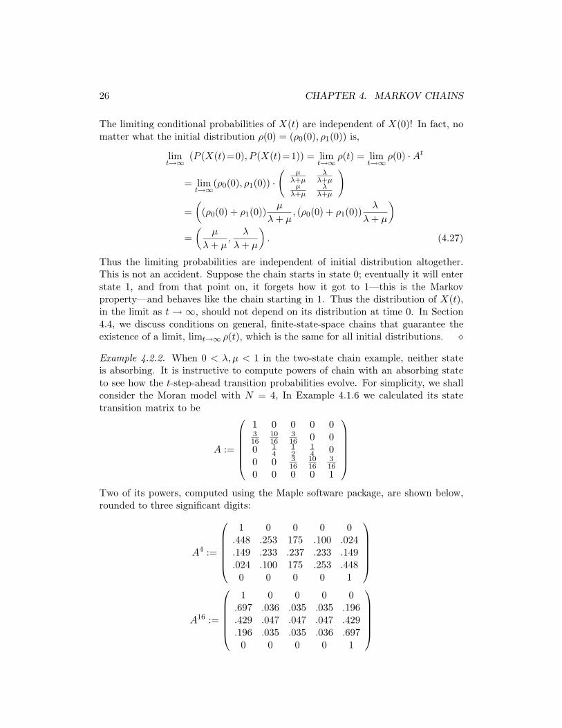
Thus the limiting probabilities are independent of initial distribution altogether.This is not an accident. Suppose the chain starts in state 0; eventually it will enterstate 1, and from that point on, it forgets how it got to 1—this is the Markovproperty—and behaves like the chain starting in 1. Thus the distribution of X(t),in the limit as t → ∞, should not depend on its distribution at time 0. In Section4.4, we discuss conditions on general, finite-state-space chains that guarantee theexistence of a limit, limt→∞ ρ(t), which is the same for all initial distributions. �
Example 4.2.2. When 0 < λ, µ < 1 in the two-state chain example, neither stateis absorbing. It is instructive to compute powers of chain with an absorbing stateto see how the t-step-ahead transition probabilities evolve. For simplicity, we shallconsider the Moran model with N = 4, In Example 4.1.6 we calculated its statetransition matrix to be
A :=
1 0 0 0 0316
1016
316 0 0
0 14
12
14 0
0 0 316
1016
316
0 0 0 0 1
Two of its powers, computed using the Maple software package, are shown below,rounded to three significant digits:
A4 :=
1 0 0 0 0
.448 .253 175 .100 .024
.149 .233 .237 .233 .149
.024 .100 175 .253 .4480 0 0 0 1
A16 :=
1 0 0 0 0
.697 .036 .035 .035 .196
.429 .047 .047 .047 .429
.196 .035 .035 .036 .6970 0 0 0 1
4.2. COMPUTATION WITH CHAINS 27
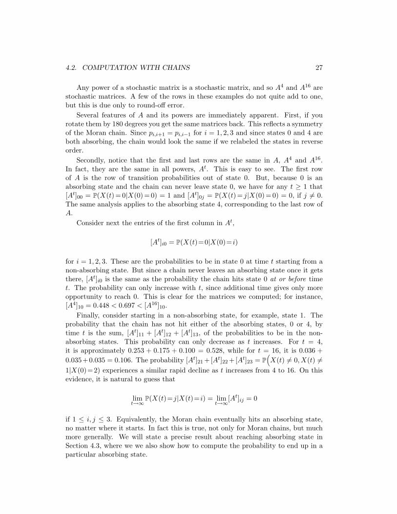
Any power of a stochastic matrix is a stochastic matrix, and so A4 and A16 arestochastic matrices. A few of the rows in these examples do not quite add to one,but this is due only to round-off error.
Several features of A and its powers are immediately apparent. First, if yourotate them by 180 degrees you get the same matrices back. This reflects a symmetryof the Moran chain. Since pi,i+1 = pi,i−1 for i = 1, 2, 3 and since states 0 and 4 areboth absorbing, the chain would look the same if we relabeled the states in reverseorder.
Secondly, notice that the first and last rows are the same in A, A4 and A16.In fact, they are the same in all powers, At. This is easy to see. The first rowof A is the row of transition probabilities out of state 0. But, because 0 is anabsorbing state and the chain can never leave state 0, we have for any t ≥ 1 that[At]00 = P(X(t)=0|X(0)=0) = 1 and [At]0j = P(X(t)= j|X(0)=0) = 0, if j 6= 0.The same analysis applies to the absorbing state 4, corresponding to the last row ofA.
Consider next the entries of the first column in At,
[At]i0 = P(X(t)=0|X(0)= i)
for i = 1, 2, 3. These are the probabilities to be in state 0 at time t starting from anon-absorbing state. But since a chain never leaves an absorbing state once it getsthere, [At]i0 is the same as the probability the chain hits state 0 at or before timet. The probability can only increase with t, since additional time gives only moreopportunity to reach 0. This is clear for the matrices we computed; for instance,[A4]10 = 0.448 < 0.697 < [A16]10.
Finally, consider starting in a non-absorbing state, for example, state 1. Theprobability that the chain has not hit either of the absorbing states, 0 or 4, bytime t is the sum, [At]11 + [At]12 + [At]13, of the probabilities to be in the non-absorbing states. This probability can only decrease as t increases. For t = 4,it is approximately 0.253 + 0.175 + 0.100 = 0.528, while for t = 16, it is 0.036 +0.035+0.035 = 0.106. The probability [At]21 +[At]22 +[At]23 = P
(X(t) 6= 0, X(t) 6=
1|X(0)=2) experiences a similar rapid decline as t increases from 4 to 16. On thisevidence, it is natural to guess that
limt→∞
P(X(t)=j|X(t)= i) = limt→∞
[At]ij = 0
if 1 ≤ i, j ≤ 3. Equivalently, the Moran chain eventually hits an absorbing state,no matter where it starts. In fact this is true, not only for Moran chains, but muchmore generally. We will state a precise result about reaching absorbing state inSection 4.3, where we we also show how to compute the probability to end up in aparticular absorbing state.
28 CHAPTER 4. MARKOV CHAINS
4.2.2 Expectations for Markov chains.
Conditional expectations and expectations are also simple to compute for Markovchains, and the formulas for doing so can again be expressed in the language ofmatrix algebra.
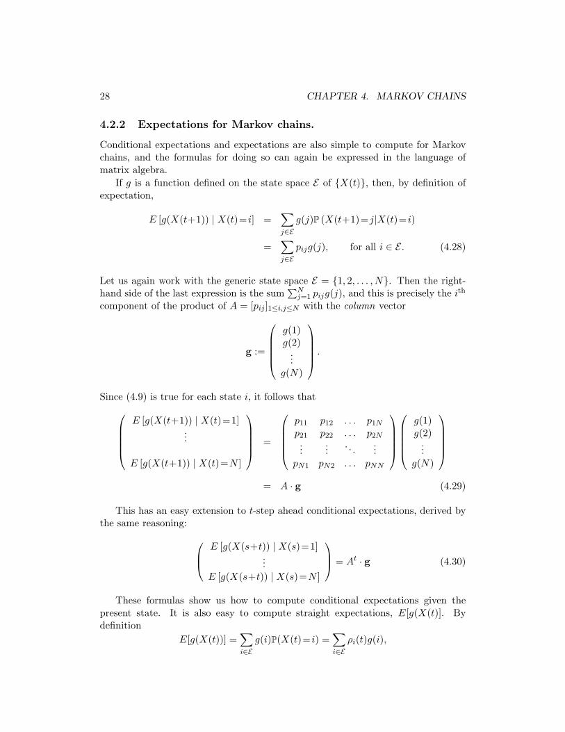
If g is a function defined on the state space E of {X(t)}, then, by definition ofexpectation,
E [g(X(t+1)) | X(t)= i] =∑j∈E
g(j)P (X(t+1)=j|X(t)= i)
=∑j∈E
pijg(j), for all i ∈ E . (4.28)
Let us again work with the generic state space E = {1, 2, . . . , N}. Then the right-hand side of the last expression is the sum
∑Nj=1 pijg(j), and this is precisely the ith
component of the product of A = [pij ]1≤i,j≤N with the column vector
g :=
g(1)g(2)
...g(N)
.
Since (4.9) is true for each state i, it follows thatE [g(X(t+1)) | X(t)=1]
...
E [g(X(t+1)) | X(t)=N ]
=
p11 p12 . . . p1N
p21 p22 . . . p2N...
.... . .
...pN1 pN2 . . . pNN
g(1)g(2)
...g(N)
= A · g (4.29)
This has an easy extension to t-step ahead conditional expectations, derived bythe same reasoning: E [g(X(s+t)) | X(s)=1]
...E [g(X(s+t)) | X(s)=N ]
= At · g (4.30)
These formulas show us how to compute conditional expectations given thepresent state. It is also easy to compute straight expectations, E[g(X(t)]. Bydefinition
E[g(X(t))] =∑i∈E
g(i)P(X(t)= i) =∑i∈E
ρi(t)g(i),
4.2. COMPUTATION WITH CHAINS 29
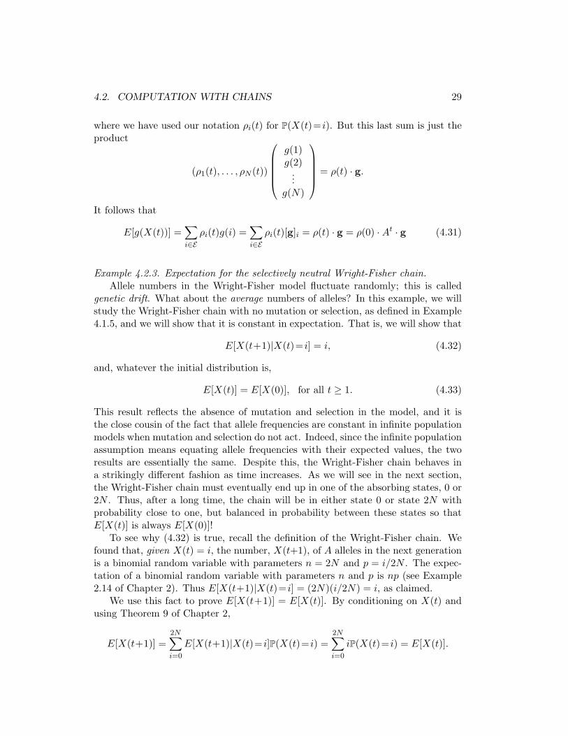
where we have used our notation ρi(t) for P(X(t)= i). But this last sum is just theproduct
(ρ1(t), . . . , ρN (t))
g(1)g(2)
...g(N)
= ρ(t) · g.
It follows that
E[g(X(t))] =∑i∈E
ρi(t)g(i) =∑i∈E
ρi(t)[g]i = ρ(t) · g = ρ(0) ·At · g (4.31)
Example 4.2.3. Expectation for the selectively neutral Wright-Fisher chain.Allele numbers in the Wright-Fisher model fluctuate randomly; this is called
genetic drift. What about the average numbers of alleles? In this example, we willstudy the Wright-Fisher chain with no mutation or selection, as defined in Example4.1.5, and we will show that it is constant in expectation. That is, we will show that
E[X(t+1)|X(t)= i] = i, (4.32)
and, whatever the initial distribution is,
E[X(t)] = E[X(0)], for all t ≥ 1. (4.33)
This result reflects the absence of mutation and selection in the model, and it isthe close cousin of the fact that allele frequencies are constant in infinite populationmodels when mutation and selection do not act. Indeed, since the infinite populationassumption means equating allele frequencies with their expected values, the tworesults are essentially the same. Despite this, the Wright-Fisher chain behaves ina strikingly different fashion as time increases. As we will see in the next section,the Wright-Fisher chain must eventually end up in one of the absorbing states, 0 or2N . Thus, after a long time, the chain will be in either state 0 or state 2N withprobability close to one, but balanced in probability between these states so thatE[X(t)] is always E[X(0)]!
To see why (4.32) is true, recall the definition of the Wright-Fisher chain. Wefound that, given X(t) = i, the number, X(t+1), of A alleles in the next generationis a binomial random variable with parameters n = 2N and p = i/2N . The expec-tation of a binomial random variable with parameters n and p is np (see Example2.14 of Chapter 2). Thus E[X(t+1)|X(t)= i] = (2N)(i/2N) = i, as claimed.
We use this fact to prove E[X(t+1)] = E[X(t)]. By conditioning on X(t) andusing Theorem 9 of Chapter 2,
E[X(t+1)] =2N∑i=0
E[X(t+1)|X(t)= i]P(X(t)= i) =2N∑i=0
iP(X(t)= i) = E[X(t)].
30 CHAPTER 4. MARKOV CHAINS
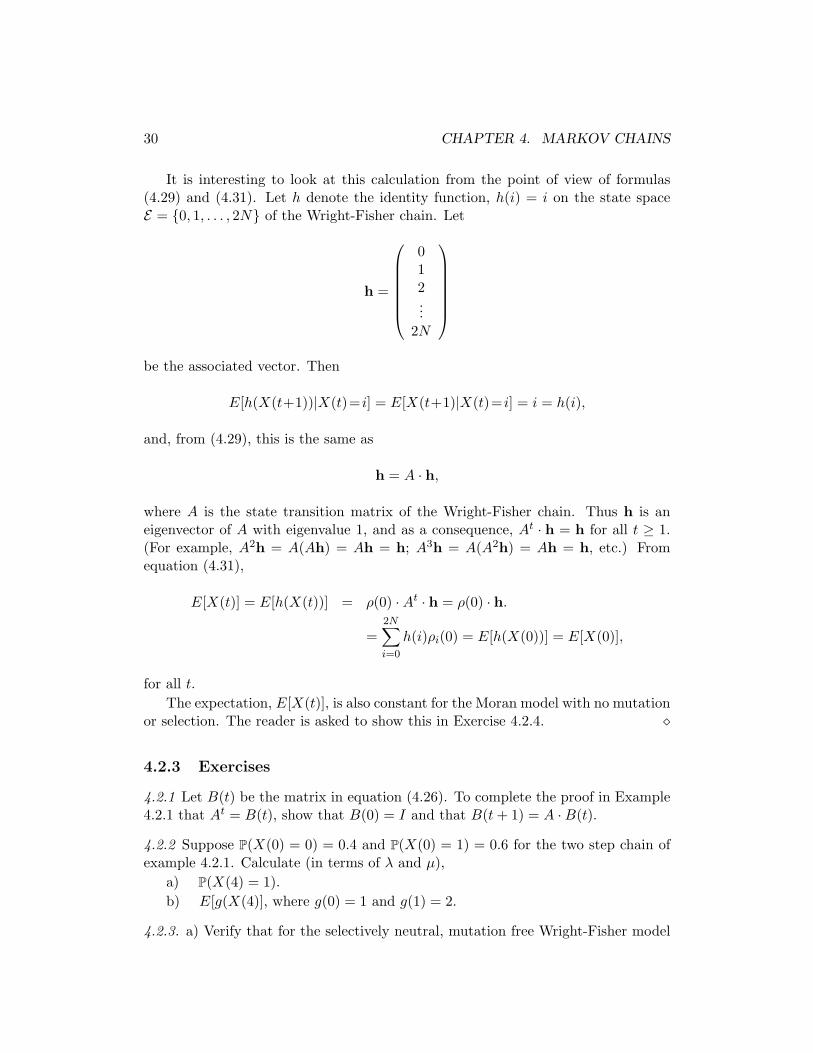
It is interesting to look at this calculation from the point of view of formulas(4.29) and (4.31). Let h denote the identity function, h(i) = i on the state spaceE = {0, 1, . . . , 2N} of the Wright-Fisher chain. Let
h =
012...
2N
be the associated vector. Then
E[h(X(t+1))|X(t)= i] = E[X(t+1)|X(t)= i] = i = h(i),
and, from (4.29), this is the same as
h = A · h,
where A is the state transition matrix of the Wright-Fisher chain. Thus h is aneigenvector of A with eigenvalue 1, and as a consequence, At · h = h for all t ≥ 1.(For example, A2h = A(Ah) = Ah = h; A3h = A(A2h) = Ah = h, etc.) Fromequation (4.31),
E[X(t)] = E[h(X(t))] = ρ(0) ·At · h = ρ(0) · h.
=2N∑i=0
h(i)ρi(0) = E[h(X(0))] = E[X(0)],
for all t.The expectation, E[X(t)], is also constant for the Moran model with no mutation
or selection. The reader is asked to show this in Exercise 4.2.4. �
4.2.3 Exercises
4.2.1 Let B(t) be the matrix in equation (4.26). To complete the proof in Example4.2.1 that At = B(t), show that B(0) = I and that B(t + 1) = A ·B(t).
4.2.2 Suppose P(X(0) = 0) = 0.4 and P(X(0) = 1) = 0.6 for the two step chain ofexample 4.2.1. Calculate (in terms of λ and µ),
a) P(X(4) = 1).b) E[g(X(4)], where g(0) = 1 and g(1) = 2.
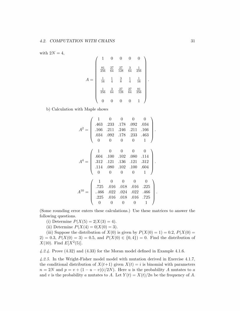
4.2.3. a) Verify that for the selectively neutral, mutation free Wright-Fisher model
4.2. COMPUTATION WITH CHAINS 31
with 2N = 4,
A =
1 0 0 0 0
81256
2764
27128
364
1256
116
14
38
14
116
1256
364
27128
2764
81256
0 0 0 0 1
.
b) Calculation with Maple shows
A2 =
1 0 0 0 0
.463 .233 .178 .092 .034
.166 .211 .246 .211 .166
.034 .092 .178 .233 .4630 0 0 0 1
.
A4 =
1 0 0 0 0
.604 .100 .102 .080 .114
.312 .121 .136 .121 .312
.114 .080 .102 .100 .6040 0 0 0 1
.
A10 =
1 0 0 0 0
.725 .016 .018 .016 .225..466 .022 .024 .022 .466.225 .016 .018 .016 .7250 0 0 0 1
.
(Some rounding error enters these calculations.) Use these matrices to answer thefollowing questions.
(i) Determine P (X(5) = 2|X(3) = 4).(ii) Determine P (X(4) = 0|X(0) = 3).(iii) Suppose the distribution of X(0) is given by P (X(0) = 1) = 0.2, P (X(0) =
2) = 0.3, P (X(0) = 3) = 0.5, and P (X(0) ∈ {0, 4}) = 0. Find the distribution ofX(10). Find E[X2(5)].
4.2.4. Prove (4.32) and (4.33) for the Moran model defined in Example 4.1.6.
4.2.5. In the Wright-Fisher model model with mutation derived in Exercise 4.1.7,the conditional distribution of X(t+1) given X(t) = i is binomial with parametersn = 2N and p = v + (1 − u − v)(i/2N). Here u is the probability A mutates to aand v is the probability a mutates to A. Let Y (t) = X(t)/2n be the frequency of A.
32 CHAPTER 4. MARKOV CHAINS
Show that E[Y (t+1)] = v + (1 − u − v)E[Y (t)]. (Compare to the mutation modelof Section 3.3.5). Find limt→∞E[Y (t)].
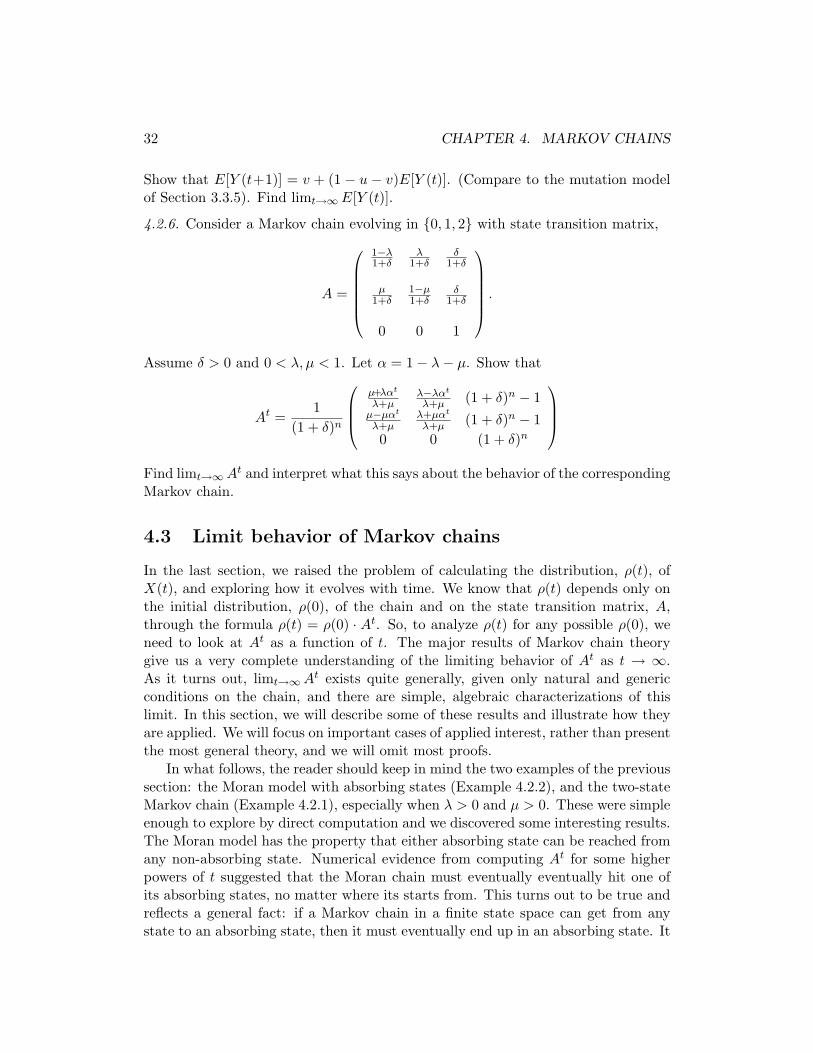
4.2.6. Consider a Markov chain evolving in {0, 1, 2} with state transition matrix,
A =
1−λ1+δ
λ1+δ
δ1+δ
µ1+δ
1−µ1+δ
δ1+δ
0 0 1
.
Assume δ > 0 and 0 < λ, µ < 1. Let α = 1− λ− µ. Show that
At =1
(1 + δ)n
µ+λαt
λ+µλ−λαt
λ+µ (1 + δ)n − 1µ−µαt
λ+µλ+µαt
λ+µ (1 + δ)n − 10 0 (1 + δ)n
Find limt→∞At and interpret what this says about the behavior of the correspondingMarkov chain.
4.3 Limit behavior of Markov chains
In the last section, we raised the problem of calculating the distribution, ρ(t), ofX(t), and exploring how it evolves with time. We know that ρ(t) depends only onthe initial distribution, ρ(0), of the chain and on the state transition matrix, A,through the formula ρ(t) = ρ(0) · At. So, to analyze ρ(t) for any possible ρ(0), weneed to look at At as a function of t. The major results of Markov chain theorygive us a very complete understanding of the limiting behavior of At as t → ∞.As it turns out, limt→∞At exists quite generally, given only natural and genericconditions on the chain, and there are simple, algebraic characterizations of thislimit. In this section, we will describe some of these results and illustrate how theyare applied. We will focus on important cases of applied interest, rather than presentthe most general theory, and we will omit most proofs.
In what follows, the reader should keep in mind the two examples of the previoussection: the Moran model with absorbing states (Example 4.2.2), and the two-stateMarkov chain (Example 4.2.1), especially when λ > 0 and µ > 0. These were simpleenough to explore by direct computation and we discovered some interesting results.The Moran model has the property that either absorbing state can be reached fromany non-absorbing state. Numerical evidence from computing At for some higherpowers of t suggested that the Moran chain must eventually eventually hit one ofits absorbing states, no matter where its starts from. This turns out to be true andreflects a general fact: if a Markov chain in a finite state space can get from anystate to an absorbing state, then it must eventually end up in an absorbing state. It
4.3. LIMIT BEHAVIOR OF MARKOV CHAINS 33
cannot knock about in the non-absorbing states forever. We discuss this in Section4.3.2, where we also show how to compute the probability to end up in a particularabsorbing state.
In contrast, the two-state chain, when both p01 = λ > 0 and p10 = µ > 0,has no absorbing states. In this case we were able to to compute At exactly andto calculate limt→∞At. We found as a consequence that a limiting distributionlimt→∞
(P(X(0) = 0), P(X(0) = 0)
)exists and is independent of the initial state
of the chain. This also reflects a general fact: in a finite state space chain whichcan move between any two states, the distribution of X(t) settles down to a limitindependent of its initial distribution. More is true: the average amount of timespent by the chain in state i tends to the limiting probability to be in i, in the infinitetime limit. This is a generalization to Markov chains of the law of large numbersand is known as an ergodic theorem. This theory is treated in Section 4.3.3.
4.3.1 Classification of states.
The long-time behavior of a Markov chain will obviously depend on the possibleways it can move among its states. We have seen this already in the differencebetween the Moran model with absorbing states of Example 4.2.2 and the two statechain without absorbing states. This section introduces more refined distinctionsbetween states, based on the way in which the chain visits them.
The definitions of this section will be based on the concept of the hitting time ofa state. For any state i, let Ti denote the first time t, t = 1, 2, . . . at which X(t) = i;if the chain never hits i for t ≥ 1, set Ti = ∞. Mathematically,
Ti := min{t; t ≥ 1 and X(t)= i}.
We emphasize that when X(0)= i, Ti is the first time after t = 0, at which the chainreturns to i.
When i and j are different states. j is said to be accessible from i, written i → j,if
P(Tj < ∞|X(0) = i) > 0.
In words, j is accessible from i if, when starting from i, the chain eventually hitsj with a positive probability. It is fairly easy to check accessibility. Suppose thereis a path, {i = i0, i1, . . . , im−1, im = j}, connecting i to j, along which pik,ik+1
> 0for every pair of successive states. Then, using the formula for the probability of apath from Theorem 1,
P(X(m)=j, X(m−1)= im−1, . . . , X(1)= i1
∣∣∣X(0)= i)
= pi0,i1 . . . pim−1,j > 0,
and hence j is accessible from i. In fact, it is clear that i → j if and only if such apath exists. Equivalently i → j if and only if j can be reached from i by followingarrows in the state transition diagram.
34 CHAPTER 4. MARKOV CHAINS
If i → j and j → i, then we say states i and j communicate and we write i ∼ j.As a matter of convention we say that i communicates with itself (i ∼ i).
Examples 4.3.1. (a) If i is absorbing, then no other state is accessible from i, andso no other states can communicate with i.
(b) Consider the Moran model without mutation in the state space {0, 1, . . . , N}.States 0 and N are absorbing states. Let i and j be any non-absorbing states.Without loss of generality, assume 0 < i < j < N . They are connected by thesimple paths
{i, i + 1, . . . , j − 1, j} and, in reverse, {j, j − 1, . . . , i + 1, i}.
But for every non-absorbing state k in the Moran models, pk,k+1 and pk,k−1 areboth positive. Hence pi,i+1 · · · pj−1,j and pj,j−1 · · · pi+1,i are both positive, and i ∼ j.From every state i, except i=N , {i, i− 1, . . . , 1, 0} is a path of positive probability.Thus i → 0 as long as i 6= N . Similarly, i → N , as long as i 6= 0.
The situation is similar for the Wright-Fisher chain without mutation. In thiscase the state space is {0, 1, . . . , 2N}, states 0 and 2N are absorbing, and pij > 0as long as i is not 0 or 2N . Thus, if 1 ≤ i ≤ 2N − 1 and j is any other state, i → j,and any two, non-absorbing states communicate. �
A state i is said to be recurrent if
P(Ti < ∞|X(0)= i) = 1;
in words, when i is recurrent, a chain starting out in state i must return to i at alater time with probability one, (since {Ti < ∞} is the event of at least one returnto i). A state that is not recurrent is said to be transient. The terms recurrent andtransient are justified by the following theorem.
Theorem 4 If i is transient, {X(t)} visits i only finitely many times with proba-bility one.
If X(0) = i, and i is recurrent, then {X(t)} visits i infinitely often with proba-bility one.
A full proof of this result is given at the end of this section, but it is easyto understand intuitively. Because of the Markov property and the assumption oftime-homogeneity, the probabilistic behavior of the chain after a visit to i is justthe same as if it started in i at time t = 0. In other words, the chain starts over aschain beginning in state i, after each return to state i. If i is recurrent and X(0)= i,the chain must return to i at least once, by definition. But then once it gets toi, it restarts as a chain beginning in i, and, by recurrence, must return again. Byrepeating this argument ad infinitum, it must return infinitely often.
If a state i is recurrent, it is interesting to ask how long the first return to itakes on average; this is the conditional expectation, E[Ti|X(0)= i]. It can happen
4.3. LIMIT BEHAVIOR OF MARKOV CHAINS 35
that this expected time is infinite, even though a return to i must take place. Thismay seem counterintuitive, but it is the case, for example, with simple, symmetricrandom walk, as we will show later. To distinguish between finite and infiniteexpected return times, we say that a state i is positive recurrent if it is recurrentand if E[Ti|X(0) = i] < ∞. On the other hand a state i is null recurrent if it isrecurrent and E[Ti|X(0)= i] = ∞.
If all the states of a Markov chain are positive (respectively, null) recurrent, thenthe chain itself is said to be positive (respectively, null) recurrent.
Examples 4.3.2. (a) Any absorbing state i, is positive recurrent, because then P(Ti =1|X(0)= i) = 1 and so E[Ti|X(0)= i] = 1.
(b) All the non-absorbing states in the Moran model without mutation are tran-sient. For suppose the chain starts in any non-absorbing state, i . Clearly, there isa positive probability it ends up in an an absorbing state, and once that happensit cannot return to i. Hence, the probability of return to i is less than 1, and i istransient.
(c) Consider the two-state chain with p01 = λ > 0 and p10 = µ > 0. Theseconditions mean the probabilities to reach 1 from 0 and 0 from 1 are both positive,and hence 0 ∼ 1. We will show later in this section that
E[T0|X(0)=0] =λ + µ
µ. (4.34)
By interchanging the roles of µ and λ, it follows likewise that
E[T1|X(0)=1] =λ + µ
λ. (4.35)
Thus, both i and j are positive recurrent.It is interesting to relate these mean return times to the limiting probabilities
derived in Example 4.2.1. There we showed that
limt→∞
(P (X(t)=0|X(0)=0), P (X(t)=1|X(0)=1)
)=( µ
λ + µ,
λ
λ + µ
)From equations (4.34) and (4.35), it follows that
limt→∞
P (X(t)=0) =1
E[T0|X(0)=0]and lim
t→∞P (X(t)=0) =
1E[T1|X(0)=1]
.
(4.36)Thus, the limiting probability to be in each state is is the inverse of the mean returntime for that state. This makes perfect sense. Intuitively, as time elapses the chainwill visit i once in every E[Ti|X(0)= i] time steps, on average, and so the probabilityto be in state i should be (E[Ti|X(0)= i])−1. This relationship between mean returntime and limiting probability holds in general in chains with communicating states,a fact we shall explain in Section 4.3.3. �
The following theorem collects some other basic facts about transient and recur-rent states that are important to know.
36 CHAPTER 4. MARKOV CHAINS
Theorem 5 (i) A recurrent state i in a Markov chain evolving in a finite statespace is automatically positive recurrent.
(ii) If i ∼ j, then states i and j are either both transient, both positive recurrent,or both null recurrent.
(iii) If all the states of a finite state space Markov chain communicate, the chainis positive recurrent.
This theorem helps make life easy, at least when life requires the analysis ofMarkov chains! For example, consider the Wright-Fisher or Moran model withmutation, when the probability of mutation from A to a and from a to A are bothpositive. The transition probabilities for these cases were derived in Exercises 4.1.6and 4.1.7. The possibility of mutation prevents the possibility of absorbing states,and it is easy to see that i ∼ j for any two states. Without further work, we deducefrom Theorem 5 that both these chains are positive recurrent.
We will not prove all the statements of Theorem 5, but they are mostly intuitive.For example, consider two communicating state i and j. Starting from i, we knowfrom Theorem 4 that the chain returns to i infinitely often. In each excursion fromi back to i, there is some positive chance to hit j. Just as an infinite sequence ofindependent coin tosses must produce an infinite number of heads if the probabilityof heads is positive, an infinite number of the excursions from i back to i must includea visit to j. Thus the chain visits j infinitely often, and so j is also recurrent.
Moreover, statement (iii) of the theorem is direct consequence of the first two.A Markov chain evolving in a finite state space must visit at least one of its statesinfinitely often, and by statements (i) and (ii) of the theorem, that state must bepositive recurrent. But if all states communicate, then they must all be positiverecurrent.
The remainder of this section supplies the derivation of equations (4.34) and (4.35), andthe proof of Theorem 4. It is optional, but recommended.
Derivation of equations (4.34) and (4.35).
Suppose X(0) = 0. Since 0 and 1 are the only states, the first time, T1, to hit state 1is also the first time the chain exists state 0. Now, T1 > s if and only if X(1) = 0, X(2) =0, . . . , X(s) = 0. Thus
P(T1 > s∣∣X(0)=0) = P
(X(1)=0, X(2)=0, . . . , X(s) = 0
∣∣∣X(0) = 0)
= ps00 = (1− λ)s. (4.37)
This means that, given X(0)=0, T1 is a geometric random variable with parameter p = λ—see, Chapter 2, pages 17 and 18. In particular, since 0 < λ by assumption, and hence0 ≤ 1− λ < 1, it follows that
P(T1 =∞
∣∣X(0)=0) = lims→∞
P(T1 > s
∣∣X(0)=0) = lims→∞
(1− λ)s = 0.
4.3. LIMIT BEHAVIOR OF MARKOV CHAINS 37
This means that the chain cannot stay in state 0 forever; it must eventually move to state1. In addition, because the expected value of a geometric random variable with parameterp is 1/p (see Chapter 2, page 34),
E[T1
∣∣X(0)=0] =1λ
. (4.38)
The same type of reasoning applied using the assumption that µ > 0, shows that, givenX(0) = 1, the first time T0 to hit 0 is a geometric random variable, and hence P(T0 <∞∣∣X(0)=1) = 1, and
E[T0
∣∣X(0)=1] =1µ
. (4.39)
Now consider the chain starting in state 0. It must eventually hit 1. But we have justseen the chain must leave state 1 eventually and return to 0, because µ > 0. It follows thatstate 0 is recurrent. Likewise, state 1 is recurrent, since λ > 0 implies that the chain mustreturn to 1 if it ever hits 0.
The first step in computing E[T0
∣∣X(0)=0] explicitly, is to condition on the state X(1)that the Markov chain moves to starting from X(0) = 0. Since it moves from 0 to 1 withprobability λ and stays at 0 with probability 1− λ,
E[T0
∣∣X(0)=0]
= E[T0
∣∣X(1)=0, X(0)=0](1− λ) + E[T0
∣∣X(1)=1, X(0)=0]λ.
Now, in the last expression, E[T0
∣∣X(1)=0, X(0)=0] = 1, since {X(1)=0, X(0)=0} impliesT1 = 1. On the other hand,
E[T0
∣∣X(1)=1, X(0)=0] = 1 +1µ
,
because, according to (4.39), the expected time to return from 1 to 0 is 1/µ and this mustbe added to the first time step used in going from 0 to 1. Therefore,
E[T0
∣∣X(0)=0] = 1− λ + λ
(1 +
1µ
)=
λ + µ
µ,
as we wanted to prove. The same reasoning, but interchanging the roles of µ and λ, shows
E[T1
∣∣X(0)=1] =λ + µ
λ.
�
Proof of Theorem 4.
Let Vi denote the number visits the chain makes to state i strictly after time 0; toemphasize, if X(0)= i, the visit to i at time t = 0 is not counted in Vi.
ri = P(Ti < ∞∣∣X(0)= i).
By definition, when 0 ≤ ri < 1 when i is transient, and ri = 1 when i is recurrent. We shallshow that
P(Vi ≥ n) = rni for all n. (4.40)
38 CHAPTER 4. MARKOV CHAINS
As an immediate consequence,
P(Vi = ∞∣∣X(0)= i) = lim
n→∞P(Vi ≥ n
∣∣X(0) = i) = limn→∞
rni
={
0, if 0 ≤ ri < 1;1, if ri = 1.
It remains to show why (4.40) is true. (Incidentally, when i is transient, (4.40) impliesthat Vi + 1 is a geometric random variable.) The case, n = 1, is easy, because {Vi ≥ 1}, theevent of at least one return to i, means exactly the same thing as {Ti < ∞}. Thus
P(Vi ≥ 1∣∣X(0)= i) = P(Ti < ∞
∣∣X(0)= i) = ri.
Next consider the event {Vi ≥ n+1}. If this happens, the time Ti of first return to i isfinite, and so from the rule of total probabilities,
P(Vi ≥ n+1
∣∣X(0)= i)
=∞∑
t=1
P(Vi ≥ n+1
∣∣Ti = t, X(0)= i)P(Ti = t
∣∣X(0)= i). (4.41)
Now, given {Ti = t}, the chain returns to i at least n + 1 times if and only if it makes atleast n visits to i after time t: Thus,
P(Vi ≥ n+1
∣∣Ti = t, X(0)= i)
= P(at least n visits to i after time t
∣∣∣Ti = t, X(0)= i).
Here, we can use the Markov property: the event {Ti = t, X(0) = i} can be expressed as{X(t) = i,X(0) = i} ∩ {X(s) 6= i, if 0 < s < t}, and the event of at least n visits to i aftertime t is an event in the future beyond time t. Therefore, by the Markov property stated inTheorem 2, only {X(t)= i} is relevant to the conditional probability, and
P(at least n visits to i after time t
∣∣∣Ti = t, X(0)= i)
= P(at least n visits to i after time t
∣∣∣X(t)= i).
But, because {X(t)} is a time-homogeneous chain, the probability it makes at least n visitsto i after time t, given X(t)= i, is the same as the probability it makes at least n visits to iafter t = 0, given X(0)=0. In other words,
P(at least n visits to i after time t
∣∣∣X(t)= i)
= P(Vi ≥ n
∣∣X(0)=0).
Note that the right-hand side does not depend on t! Therefore, it follows from equation(4.41) that
P(Vi ≥ n+1
∣∣X(0)= i)
=∞∑
t=1
P(Vi ≥ n
∣∣X(0)= i)P(Ti = t
∣∣X(0)= i)
= P(Vi ≥ n
∣∣X(0)= i) ∞∑
t=1
P(Ti = t∣∣X(0)= i)
= P(Vi ≥ n
∣∣X(0)= i)P(Ti < ∞
∣∣X(0)= i)
= riP(Vi ≥ n
∣∣X(0)= i).
This says that if we let an := P(Vi ≥ n
∣∣X(0) = i), {an} satisfies the simple difference
equation an+1 = rian. Since a1 = P(Vi ≥ 1
∣∣X(0)= i)
= ri, the solution is P(Vi ≥ n
∣∣X(0)=i)
= an = rni , and this is what we wanted to prove.
4.3. LIMIT BEHAVIOR OF MARKOV CHAINS 39
4.3.2 Chains with absorbing states
In this section we discuss we discuss finite state-space Markov chains with the prop-erty that it is possible to hit an absorbing state no matter where the chain starts.The guiding examples are the Moran and Wright-Fisher models without mutation.
In the discussion, E will denote the (finite) state space of a chain and S willdenote the subset of its absorbing states. As usual, A denotes its state transitionmatrix. If i is any state and if a is an absorbing state, let
gai = P
(X(t)=a for some t ≥ 0
∣∣∣X(0)= i).
This is the probability the chain eventually gets absorbed by state a given that itstarts in state i. For the Wright-Fisher model in a population of size N , the twoabsorbing states are 0 and 2N , and the event of getting absorbed into one of themis called fixation, because when it occurs, either allele A disappears (absorption intostate 0) or takes over (absorption into state 2N). Then g0
i and g2Ni are the proba-
bilities of absorption into these two alternatives starting from i, and are interestingto know from the biological point of view.
If a is an absorbing state, the probability the chain gets absorbed into state aby time t, when it starts in i, is simply the probability
P(X(t)=a|X(0)= i) = [At]ia.
because once the chain arrives at a, it stays there. The probability to be eventuallyabsorbed in a is the limit as t → ∞ of the probability to be absorbed by time t.Thus
gai = lim
t→∞P(X(t)=a|X(0)= i) = lim
t→∞[At]ia.
The probability of starting in i and eventually getting to some absorbing state is
P(eventual absorption
∣∣∣X(0)= i) =∑a∈S
gai .
Theorem 6 Let {X(t)} be a Markov chain in a finite state space E. Assume thatthe set of absorbing state S is not empty and assume that for every non-absorbingstate i, there exists an absorbing state a ∈ S, such that a is accessible from i. LetT = E − S be the set of all non-absorbing states.
Then
(i) Every state i ∈ T is transient.
(ii) For every i ∈ T ,∑a∈S
gai = 1. (Absorption occurs with probability one no
matter where the chain starts.)
(iii) If j ∈ T , then limt→∞
[At]ij = 0, for all i ∈ E.

40 CHAPTER 4. MARKOV CHAINS
(iv) For each a, {gai ; i ∈ E} is the unique solution to
gaa = 1 and ga
s = 0 if s ∈ S and s 6= a; (4.42)gai =
∑j∈E
pijgaj =
∑j∈T
pijgaj + pia (4.43)
The important qualitative result of this theorem is that a chain must eventuallyenter an absorbing state, if it evolves in a finite state space with only transientand absorbing states. The Wright-Fisher and Moran models without mutation bothsatisfy the hypotheses of Theorem 6, and thus fixation must ultimately occur inboth models. Thus, in the absence of mutation, an allele will eventually either takeover or disappear from the population, just due to chance.
The important quantitative result of the theorem is the system of linear equationsfor absorption probabilities stated in part (iv). They enable us, in principle, to findthe probability with which the chain ends up in a particular absorbing state. Infact, the derivation in Section 4.1.4 of the probability of ruin in the gambler’s ruinproblem is an example of the equations in part (iv).
Statements (i) of the theorem is immediate from the definition of transience.By assumption, if i is not an absorbing state, a chain starting in state i can reachan absorbing state with positive probability, and therefore the probability that itreturns to i is less than one. From Theorem 4, we know that the chain can visit atransient state only finite many times, and, since there are only a finite number oftransient state—because the state space is finite—the chain starting in any transientstate must eventually hit an absorbing state. This implies statement (ii), because∑a∈S
gai is the probability to hit eventually an absorbing state, starting from i, and
it also implies statement (iii), because if the probability of hitting some absorbingstate eventually is one, the limiting probability to be in any transient state goes to0 as t →∞.
Rather than justify statement (iv) generally, we will explain and use equations(4.42) and (4.43) in an example.
Example 4.3.3. Absorption probabilities for the Moran Model with no mutation whenN = 4.
The state space for this example is E = {0, 1, 2, 3, 4} and the state transitionmatrix, which was computed in Example 4.2.6, is
1 0 0 0 0316
1016
316 0 0
0 14
12
14 0
0 0 316
1016
316
0 0 0 0 1
.
4.3. LIMIT BEHAVIOR OF MARKOV CHAINS 41
We are interested in computing gNi , the probability that the chain eventually hits
the absorbing state N , given that X(0) = i. We have right away that,
g40 = 0 and g4
4 = 1, (4.44)
because if X(0) = 0, the chain stays forever in state O and thus cannot reach 4, andif X(0) = 4, the chain is already in state 4 and hence never leaves. These equationsare precisely what equation (4.42) says for the case of a = 4.
Let V be the event the chain eventually hits N ; thus, g4i = P(V |X(0) = i), by
definition. Consider the case, i = 1. We will explore what happens if we try tocompute gN
1 by conditioning on the value of X(1). Note first that
P(V |X(1)=j, X(0)=1) = P(V |X(1)=j) = g4j ,
because, once X(1)= j is given, the Markov property implies X(0)=1 is no longerrelevant, and we are looking at the probability of eventually hitting state 4 startingfrom state j.
Now, if X(0) = 1, there are three possibilities for X(1); it is 0 with probabilityp10, it is 1 with probability p11 and it is 2 with probability p12, (note, p13 = p14 = 0).From the previous paragraph, if the chain arrives at 0, the probability of V is theng40 = 0; if it arrives at 1 the probability of V is then g4
1, and so on. Thus, by therule of total probabilities,
g41 = p10g
40 + p11g
41 + p12g
42 = (10/16)g4
1 + (3/16)g42 (4.45)
This is the version, for this example, of equation (4.43) of (iv) in Theorem 6 in thecase i = 1.
The reader should repeat the same type of reasoning to derive similar equationsfor i = 2 and i = 3. They are:
g42 = p21g
41 + p22g
42 + p23g
43 = (1/4)g4
1 + (1/2)g42 + (1/4)g4
3 and (4.46)g43 = p32g
42 + p33g
43 + p34g
44 = (3/16)g4
2 + (10/16)g42 + (2/16). (4.47)
(4.48)
Thus, we have derived three, linear equations for the three unknowns g41, g4
2, andg43. The reader may check that the solution is g4
1 = 1/4, g42 = 1/2, and g4
3 = 3/4. �
The method of the previous example can always be used and the reader shouldunderstand how it is derived. However, there are sometimes simpler methods. Inthe following example, we again consider the Moran model, but this time for generalN , and we derive an expression for the probability of absorption in state N . Thederivation will use the fact, proved earlier, that expectation is constant for theMoran chain, and statement (iii) of Theorem 6.
42 CHAPTER 4. MARKOV CHAINS
Example 4.3.4 Absorption probabilities for the Moran model without mutation, gen-eral N .
We showed in Exercise 4.2.4 that the expected value of the Moran chain doesnot change with time. In particular,
i = E[X(t)|X(0)= i] for all t ≥ 1.
Let us write out the expectation in terms of the conditional distribution of X(t).Thus,
i =N∑
j=0
jP(X(t)=j|X(0))= i) =N∑
j=0
j[At]ij =N∑
j=1
j[At]ij .
In the last sum, we omitted the term corresponding to j = 0 because it is automat-ically 0. If 1 ≤ j ≤ N − 1, then j is transient, and part (iii)of Theorem 6 says thatlimt→∞[At]ij = 0. On the other hand, we know from the discussion at the beginningof this section that limt→∞[At]iN = gN
i . Thus, by taking limits as t →∞,
i = limt→∞
N∑j=1
j[At]ij = NgNi .
HencegNi =
i
N, for all 0 ≤ i ≤ N.
Since 0 and N are the only absorbing states, and since absorption must take place,g0i = 1− gN
i = 1− iN .
When put in words, we get a very pleasing result: the probability that allele Aeventually takes over the population is equal to its initial frequency in the popula-tion. �
Example 4.3.5. Absorption probabilities for the Wright-Fisher chain with mutation.Consider the Wright-Fisher chain in a population of size 2N when there is no mu-tation. As we showed in the previous section, the expectation of this chain is alsoconstant in time. The same argument we just used for the Moran model shows that
g2Ni =
i
2Nfor all 0 ≤ i ≤ 2N.
The reader should repeat the argument for this case as an exercise. �
4.3.3 Ergodic theorem for recurrent Markov Chains
Stationary distributions
Let {X(t)} be a stochastic process evolving in the discrete state space E , and letρ(t) = {ρi(t); i ∈ E} denote the distribution of X(t) for each t ≥ 0; recall that, by
4.3. LIMIT BEHAVIOR OF MARKOV CHAINS 43
definition, ρi(t) := P(X(t) = i) for every i ∈ E . If ρ(t) = ρ(0) for all t ≥ 0, thenwe say that ρ(0) is a stationary distribution for {X(t)}, because it is the same forall t. Thus, while the process itself is moving around randomly from state to stateas time progresses, the probability of X(t) being in any particular state does notchange. We we usually denote the stationary distribution by π = {πi; i ∈ E}.
When {X(t)} is a Markov chain evolving in the state space E = {0, 1, . . . , N} wehave been interpreting ρ(t) as a row vector ρ(t) = (ρ0(t), ρ1(t), . . . , ρN (t)). Likewise,we think of a stationary distribution as row vector π = (π0, π1, . . . , πN ), where πi
represents the unchanging probability that X(t)= i. Notice that π must a probabilityvector ; that is π≥0 for all state i and
∑n1 πi = 1.
Now let A be a state transition matrix. We have the following very importantresult. A vector π is a stationary distribution for a Markov process with statetransition matrix A if and only if
π = π ·A (4.49)∑i∈E
πi = 1 and πi ≥ 0 for all i in E . (4.50)
The second equation, (4.50), is just the statement that π must be a probabilityvector. Suppose that it is, and assume π is a stationary distribution; that is, ρ(t) = πfor all t. Then, by using the identity ρ(t+1) = ρ(t) · A (see Theorem 3), π =ρ(t+1) = ρ(t) · A = π · A, and hence π must be a solution to (4.49). Conversely, ifπ = π · A, if π is a probability vector and if ρ(0) = π, then ρ(1) = π · A = π, henceρ(2) = ρ(1)A = πA = π, and continuing in this way by induction, ρ(t) = π for allpositive integers t. Thus, π is a stationary distribution.
From this characterization, finding a stationary distribution for a Markov chainis a matter of solving the system of linear equations given by (4.49) and (4.50).
Example 4.3.5. Consider the two state chain with λ+µ > 0. Then (4.49) and (4.50)become
(π0, π1) = (π0, π1) ·(
1−λ λµ 1−µ
)and π0 + π1 = 1.
This matrix equation is equivalent to the two equations: π0 = (1−λ)π0 + µπ1, andπ1 = λπ0 + (1−µ)π1. Both of these reduce to λπ0 = µπ1. The reader may showthat the unique solution to λπ0 = µπ1 and π0 + π1 = 1 is
(π0, π1) =( µ
λ + µ,
λ
λ + µ
). �
In the study of the two-state chain in Example 4.2.1, we found that, whateverthe initial law,
limt→∞
(P(X(t)=0), P(X(t)=1)
)=( µ
λ + µ,
λ
λ + µ
).
44 CHAPTER 4. MARKOV CHAINS
This is exactly the unique, stationary distribution we just found for the two-statechain. This is not an accident, but an illustration of an important and general fact.For any Markov chain, if π = limt→∞ ρ(t) exists, then π is a stationary distribution.Indeed, let A be the state transition matrix of the chain, and assume π = limt→∞ ρ(t)exists. Of course, if t → ∞, then t−1 → ∞ also, and so π = limt→∞ ρ(t−1). Butwe know for a Markov chain that ρ(t) = ρ(t−1) ·A. Thus,
π = limt→∞
ρ(t) = limt→∞
ρ(t−1) ·A = π ·A,
and hence π is stationary.
Periodicity of states
Consider a Markov chain {X(t)}, that, starting from state i, we can only return toi after an even number of steps, and in fact P(X(2t)= i|X(0)= i) > 0 for all t. Inthis case, we say that state i has period 2. Periodicity is an important considerationin the study of limits of distributions. If i has period 2, then it really only makessense to look at P(X(t) = i|X(0) = i) along the sequence of even times, becauseP(X(t)= i|X(0)= i) = 0 if t is odd.
More generally, the period of i is the largest integer d such that the process canreturn to i in some multiple of d time steps; mathematically, the period is the largestinteger d such that
P(Ti ∈ {d, 2d, 3d, . . .}
∣∣∣X(0)= i)
= 1.
If the period of a state is d = 1, the state is said to be aperiodic.It is clear that if pii = P(X(1)= i|X(0)= i) > 0, then state i is aperiodic. Since
pii > 0 for every i in the Moran and Wright-Fisher models, with mutation or not,all the states in these chains are aperiodic. In fact, aperiodicity is the norm for mostapplied models, and will be the only case of real interest to us. An exception is thesymmetric random walk. In this case, the chain must move up or down one unit inevery time step and so all states have period 2.
The reader should be aware of the facts stated in the following theorem. Itsproof is omitted.
Theorem 7 a) If i ∼ j, then i and j have the same period.b) If there is a positive integer t0, such that every entry of the matrix At0 is
positive, then all states communicate and are aperiodic.
The Ergodic Theorem
This is the most important theorem in the theory of Markov chains. It general-izes to positive recurrent chains all the nice properties we discovered by explicitcomputation for two-state, recurrent chains.
4.3. LIMIT BEHAVIOR OF MARKOV CHAINS 45
Theorem 8 Let A be the state transition matrix of a Markov chain. Assume allstates communicate with one another and are positive recurrent. Then
(a)) There is admits a unique stationary distribution π for the chain.(b) If, in addition, the chain is aperiodic, then
limt→∞
[At]ij = πj , for all states i and j; (4.51)
Moreover, the stationary distribution has the following two probabilistic interpreta-tions for a Markov chain {X(t)} whose state transition matrix is A:
πj =1
E[Tj |X(0)=j]for each state j, and; (4.52)
for any state j and any initial distribution of X(0),
πj = limt→∞
number of visits of X(1), X(2), . . . , X(t) to state j
t(4.53)
with probability one.Finally, no matter what the initial law of X(t) is
limt→∞
ρ(t) = π. (4.54)
Remarks.1. The statement, (4.53), in this theorem is a generalization of the law of large
numbers to Markov chains. In words, it says that the long run average number ofvisits to a state j is equal to the limiting probability, πj , to be in state j. Statementsof this type are called ergodic theorems, whence the name given to Theorem 8.
2. It should be emphasized that the statements in equations (4.51), (4.52), and(4.54) require the assumption of aperiodicity. Modified versions of these statementsare true in the periodic case, but they are not necessary for our applications.
3. No assumption about the finiteness of the state space is made in Theorem 8.It is true whenever the state space is discrete. When the state space is finite andall states communicate, then, as we have discussed, the chain is positive recurrent,and the theorem applies.
4. When the states of a chain all communicate and are all null recurrent, it canbe shown that a stationary distribution does not exist and limt→∞[At]ij = 0 for allj.
5. The matrix interpretation of (4.51) is worth noting. Let the state space beE = {0, 1, . . . , N}. Then,
limt→∞
At =
π0 π1 π2 · · · πN
π0 π1 π2 · · · πN...
......
...π0 π1 π2 · · · πN
. (4.55)
46 CHAPTER 4. MARKOV CHAINS
This form makes it very clear that limt→∞ P(X(t)= j|X(0)= i
)= limt→∞[At]ij is
independent of the starting state, i.
We have demonstrated all the claims of Theorem 8, except for statement (4.53),for the two-state chain, and I recommend that the reader review this analysis. AA proof of Theorem 8 for the general case is beyond the scope of this text, and isomitted. We only note here that (4.54) is a consequence of (4.51). Indeed, fromformula (4.24), we know that for a general initial law, ρ(0) of X(0),
P(X(t)=j) =∑i∈E
ρ(i)[At]ij .
By taking a limit on both sides and exchanging limit and summation,
limt→∞
P(X(t)=j) =∑i∈E
ρi(0) limt→∞
[At]ij
=∑i∈E
ρi(0)πj = πj
∑i∈E
ρi(0)
= πj .
(The last step follows because ρ(0) is a probability distribution on E , and hence∑i∈E ρ(i) = 1.) This gives (4.54).
Example 4.3.6. Consider the Moran model with mutation as defined in Example4.6. Assume that N = 3 and u = v = 1/4. Then the probability transition matrixis
A =
3/4 1/4 0 07/36 19/36 10/36 0
0 10/36 19/36 7/360 0 1/4 3/4
.
The state space is finite and all state communicate, and hence the chain is positiverecurrent and Theorem 8 applies. The probability to be in state j will tend in thelimit as t →∞ to πj , where π = (π0, π1, π2, π3) is the unique solution to
(π0, π1, π2, π3) = (π0, π1, π2, π3)
3/4 1/4 0 07/36 19/36 10/36 0
0 10/36 19/36 7/360 0 1/4 3/4
,
and π0 + π1 + π2 + π3 = 1. The first system of equation is equivalent to
π0 =34π0 +
736
π1
π1 =14π0 +
1936
π1 +1036
π2
π2 =1036
π1 +1936
π2 +14π3
π3 =736
π2 +34π3
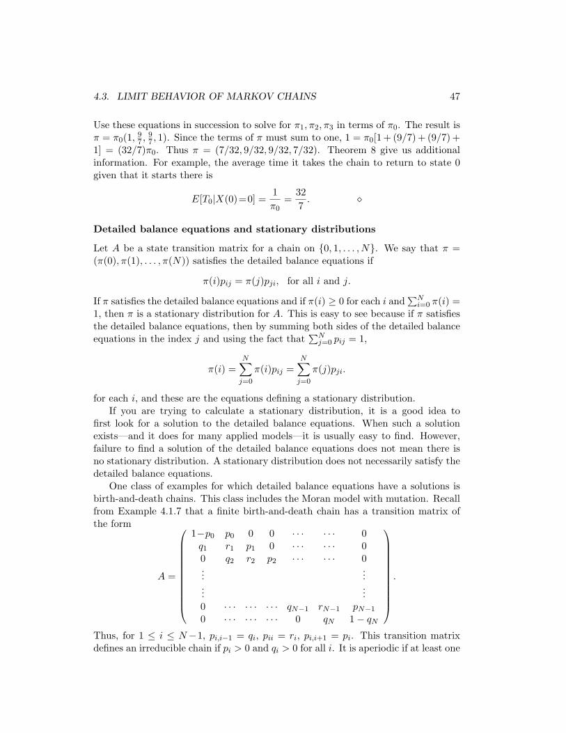
4.3. LIMIT BEHAVIOR OF MARKOV CHAINS 47
Use these equations in succession to solve for π1, π2, π3 in terms of π0. The result isπ = π0(1, 9
7 , 97 , 1). Since the terms of π must sum to one, 1 = π0[1 + (9/7) + (9/7) +
1] = (32/7)π0. Thus π = (7/32, 9/32, 9/32, 7/32). Theorem 8 give us additionalinformation. For example, the average time it takes the chain to return to state 0given that it starts there is
E[T0|X(0)=0] =1π0
=327
. �
Detailed balance equations and stationary distributions
Let A be a state transition matrix for a chain on {0, 1, . . . , N}. We say that π =(π(0), π(1), . . . , π(N)) satisfies the detailed balance equations if
π(i)pij = π(j)pji, for all i and j.
If π satisfies the detailed balance equations and if π(i) ≥ 0 for each i and∑N
i=0 π(i) =1, then π is a stationary distribution for A. This is easy to see because if π satisfiesthe detailed balance equations, then by summing both sides of the detailed balanceequations in the index j and using the fact that
∑Nj=0 pij = 1,
π(i) =N∑
j=0
π(i)pij =N∑
j=0
π(j)pji.
for each i, and these are the equations defining a stationary distribution.If you are trying to calculate a stationary distribution, it is a good idea to
first look for a solution to the detailed balance equations. When such a solutionexists—and it does for many applied models—it is usually easy to find. However,failure to find a solution of the detailed balance equations does not mean there isno stationary distribution. A stationary distribution does not necessarily satisfy thedetailed balance equations.
One class of examples for which detailed balance equations have a solutions isbirth-and-death chains. This class includes the Moran model with mutation. Recallfrom Example 4.1.7 that a finite birth-and-death chain has a transition matrix ofthe form
A =
1−p0 p0 0 0 · · · · · · 0q1 r1 p1 0 · · · · · · 00 q2 r2 p2 · · · · · · 0...
......
...0 · · · · · · · · · qN−1 rN−1 pN−1
0 · · · · · · · · · 0 qN 1− qN
.
Thus, for 1 ≤ i ≤ N−1, pi,i−1 = qi, pii = ri, pi,i+1 = pi. This transition matrixdefines an irreducible chain if pi > 0 and qi > 0 for all i. It is aperiodic if at least one
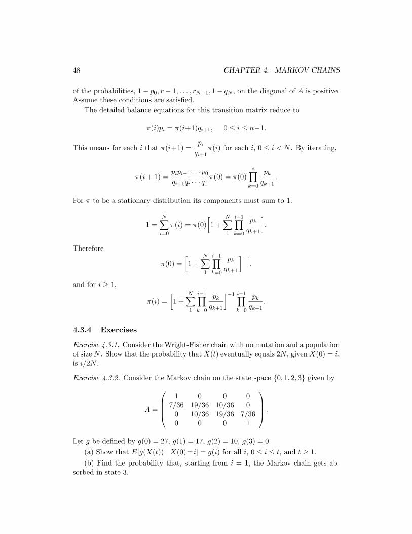
48 CHAPTER 4. MARKOV CHAINS
of the probabilities, 1− p0, r− 1, . . . , rN−1, 1− qN , on the diagonal of A is positive.Assume these conditions are satisfied.
The detailed balance equations for this transition matrix reduce to
π(i)pi = π(i+1)qi+1, 0 ≤ i ≤ n−1.
This means for each i that π(i+1) =pi
qi+1π(i) for each i, 0 ≤ i < N . By iterating,
π(i + 1) =pipi−1 · · · p0
qi+1qi · · · q1π(0) = π(0)
i∏k=0
pk
qk+1.
For π to be a stationary distribution its components must sum to 1:
1 =N∑
i=0
π(i) = π(0)[1 +
N∑1
i−1∏k=0
pk
qk+1
].
Therefore
π(0) =[1 +
N∑1
i−1∏k=0
pk
qk+1
]−1
.
and for i ≥ 1,
π(i) =[1 +
N∑1
i−1∏k=0
pk
qk+1
]−1 i−1∏k=0
pk
qk+1.
4.3.4 Exercises
Exercise 4.3.1. Consider the Wright-Fisher chain with no mutation and a populationof size N . Show that the probability that X(t) eventually equals 2N , given X(0) = i,is i/2N .
Exercise 4.3.2. Consider the Markov chain on the state space {0, 1, 2, 3} given by
A =
1 0 0 0
7/36 19/36 10/36 00 10/36 19/36 7/360 0 0 1
.
Let g be defined by g(0) = 27, g(1) = 17, g(2) = 10, g(3) = 0.(a) Show that E[g(X(t))
∣∣∣ X(0)= i] = g(i) for all i, 0 ≤ i ≤ t, and t ≥ 1.(b) Find the probability that, starting from i = 1, the Markov chain gets ab-
sorbed in state 3.
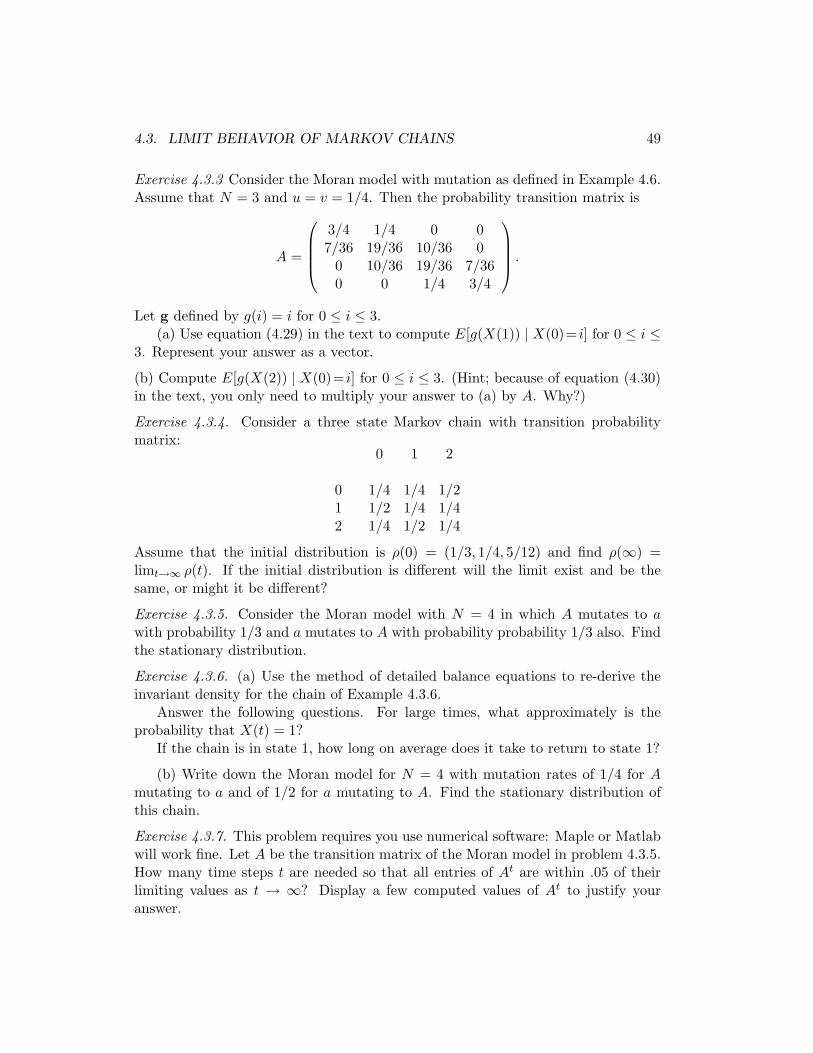
4.3. LIMIT BEHAVIOR OF MARKOV CHAINS 49
Exercise 4.3.3 Consider the Moran model with mutation as defined in Example 4.6.Assume that N = 3 and u = v = 1/4. Then the probability transition matrix is
A =
3/4 1/4 0 07/36 19/36 10/36 0
0 10/36 19/36 7/360 0 1/4 3/4
.
Let g defined by g(i) = i for 0 ≤ i ≤ 3.(a) Use equation (4.29) in the text to compute E[g(X(1)) | X(0)= i] for 0 ≤ i ≤
3. Represent your answer as a vector.
(b) Compute E[g(X(2)) | X(0)= i] for 0 ≤ i ≤ 3. (Hint; because of equation (4.30)in the text, you only need to multiply your answer to (a) by A. Why?)
Exercise 4.3.4. Consider a three state Markov chain with transition probabilitymatrix:
0 1 2
0 1/4 1/4 1/21 1/2 1/4 1/42 1/4 1/2 1/4
Assume that the initial distribution is ρ(0) = (1/3, 1/4, 5/12) and find ρ(∞) =limt→∞ ρ(t). If the initial distribution is different will the limit exist and be thesame, or might it be different?
Exercise 4.3.5. Consider the Moran model with N = 4 in which A mutates to awith probability 1/3 and a mutates to A with probability probability 1/3 also. Findthe stationary distribution.
Exercise 4.3.6. (a) Use the method of detailed balance equations to re-derive theinvariant density for the chain of Example 4.3.6.
Answer the following questions. For large times, what approximately is theprobability that X(t) = 1?
If the chain is in state 1, how long on average does it take to return to state 1?
(b) Write down the Moran model for N = 4 with mutation rates of 1/4 for Amutating to a and of 1/2 for a mutating to A. Find the stationary distribution ofthis chain.
Exercise 4.3.7. This problem requires you use numerical software: Maple or Matlabwill work fine. Let A be the transition matrix of the Moran model in problem 4.3.5.How many time steps t are needed so that all entries of At are within .05 of theirlimiting values as t → ∞? Display a few computed values of At to justify youranswer.