Embed Size (px)
Citation preview
Embedding discrete- into continuous-time Markov chains
Bachelor thesis
submitted by Leon V. S. Roschig to the
Department of Mathematics and Computer Science
Philipps-University Marburg
September 28, 2015
Supervised by
Prof. Dr. Hajo Holzmann
Contents
Introduction (English) 3
Introduction (German) 5
1 Holomorphic functional calculus 7
1.1 Preliminaries . . . . . . . . . . . . . . . . . . . . . . . . . . . . . . . . . . . . . . . . . . . 7
1.2 Integration in Banach spaces and algebras . . . . . . . . . . . . . . . . . . . . . . . . . . . 12
1.3 Holomorphic functional calculus . . . . . . . . . . . . . . . . . . . . . . . . . . . . . . . . . 26
2 Theoretical results 35
2.1 Preliminaries . . . . . . . . . . . . . . . . . . . . . . . . . . . . . . . . . . . . . . . . . . . 35
2.2 Embedding problem . . . . . . . . . . . . . . . . . . . . . . . . . . . . . . . . . . . . . . . 38
2.3 Identification problem . . . . . . . . . . . . . . . . . . . . . . . . . . . . . . . . . . . . . . 45
3 Algorithms and numerical examples 49
3.1 Algorithms to search for a generator . . . . . . . . . . . . . . . . . . . . . . . . . . . . . . 49
3.2 Numerical examples . . . . . . . . . . . . . . . . . . . . . . . . . . . . . . . . . . . . . . . 52
Bibliography 59
List of Figures 62
Introduction (English)
Markov chains are stochastic processes with certain distribution characteristics, that are used in various
fields of research and modeling. Applications include automatic speech recognition, valuation of web
pages by search engines, algorithmic music composition and, as will be discussed more intensively in this
bachelor thesis, forecasting of the credit-worthiness of a debtor.
Markov chains operate on spaces of so-called states. In this thesis, only processes with finitely many
states will be discussed. Markov chains can be divided into processes in discrete and continuous time.
The defining characteristic of a discrete-time Markov chain is its transition matrix P , which specifies the
probability of changing between the states of the process in a given time unit. The natural powers of P
allow prediction of the behavior of the chain over integer multiples of this time unit. The construction of a
continuous-time Markov chain is based on a so-called generator matrix Q. Using power series expansions,
we can generalize the exponential function to matrices and make sense of the expression P (t) := exp(tQ)
for t ≥ 0. This notion will be used to define the transition probabilities of a Markov chain in continuous
time.
Hence, sufficient knowledge of the generator Q enables us to forecast the course of the process over any
given time horizon. The resulting increase in flexibility of prediction is highly valuable to many practical
applications. To profit from this advantage, one tries to embed a discrete- into a continuous-time Markov
chain. This means that we assume a given transition matrix P of a process in discrete time to be P (1)
in a continuous-time model. We will then have to solve the central equation
P = exp(Q) ,
where P and Q are matrices with certain properties.
This identity motivates us to search for an inverse to the matrix exponential, a matrix logarithm. We
approach this task by drawing on the theory of the real and complex logarithm function. The naive
technique of substituting a matrix symbolically for a complex variable does not provide a suitable frame-
work for this idea. Therefore, we will resort to a concept of greater scope, the so-called holomorphic
functional calculus. Briefly worded, we will explain the application of functions to matrices by following
the well-known Cauchy integral formula from complex analysis, which states that
f(z) =
∫Γ
f(ζ)
ζ − zdζ
for a holomorphic function f , a complex argument z, an appropriately defined line integral and a suitable
cycle Γ.
3

Introduction (English)
It is a priori not clear, whether the central equation will be solvable at all. Hence, we will concern
ourselves with the task of finding necessary and sufficient conditions for the existence of an exact or
approximate solution, which became known as the embedding problem. Furthermore, we do not know
from the outset, if a solution to the identity will be unique. Thus, in case multiple different solutions
exist, we will have to discuss which is the ”correct” one for our application. This question is commonly
referred to as the identification problem.
We will use the results of these investigations to formulate algorithms for solving the above equation
exactly or approximately. In the end, the developed methods will be tested and compared with the help
of numerical examples from the real credit rating process.
The main source for this thesis is the paper [IRW], where certain results about the holomorphic functional
calculus are assumed to be known and, building on this, a great part of the theory for the subsequent
chapters is developed.
4
Introduction (German)
Markov-Ketten sind stochastische Prozesse mit bestimmten Verteilungseigenschaften, die in verschiedenen
Gebieten der Forschung und Modellierung verwendet werden. Anwendungsbeispiele umfassen automatis-
che Spracherkennung, Bewertung von Internetseiten durch Suchmaschinen, algorithmische Musikkompo-
sition und, wie in dieser Bachelorarbeit intensiv diskutiert wird, Prognostizierung der Kreditwurdigkeit
eines Schuldners.
Markov-Ketten operieren auf sogenannten Zustandsraumen. In dieser Arbeit werden nur Prozesse mit
endlichem Zustandsraum betrachtet. Markov-Ketten konnen in Prozesse in diskreter und stetiger Zeit un-
terteilt werden. Das definierende Charakteristikum einer zeitdiskreten Markov-Kette ist ihre Ubergangs-
matrix P , welche die Wahrscheinlichkeit angibt, innerhalb einer gegebenen Zeiteinheit zwischen den
Zustanden des Prozesses zu wechseln. Die naturlichen Potenzen von P erlauben eine Vorhersage der Ent-
wicklung des Prozesses uber ganzzahlige Vielfache der Zeiteinheit. Die Konstruktion einer zeitstetigen
Markov-Kette basiert auf einer sogenannten Erzeugermatrix Q. Mithilfe von Potenzreihendarstellungen
lasst sich die Exponentialfunktion auf Matrizen verallgemeinern und daher sinnvoll von dem Ausdruck
P (t) := exp(tQ) fur t ≥ 0 sprechen. Dieser kann dann verwendet werden, um die Ubergangswahrschein-
lichkeiten einer Markov-Kette in stetiger Zeit zu definieren.
Somit gestattet uns eine hinreichende Kenntnis des Erzeugers Q, den Verlauf des Prozesses uber einen
beliebigen Zeithorizont vorauszusagen. Die dadurch gesteigerte Flexibilitat bei der Vorhersage stellt fur
viele praktische Anwendungen eine wertvolle Bereicherung dar. Um von diesem Vorteil zu profitieren,
versucht man die zeitdiskrete in eine zeitstetige Markov-Kette einzubetten. Dies bedeutet, dass man die
Ubergangsmatrix P eines Prozesses in diskreter Zeit als P (1) in einem zeitstetigen Modell annimmt. Es
gilt dann, die zentrale Gleichung
P = exp(Q)
zu losen, wobei P und Q Matrizen mit bestimmten Eigenschaften bezeichnen.
Das motiviert uns, nach einer Umkehrfunktion zum Matrixexponential zu suchen, einem Matrixlogarith-
mus. Wir wollen diese Aufgabe dadurch angehen, dass wir auf die Theorie der reellen und komplexen Log-
arithmusfunktion zuruckgreifen. Die naive Technik, eine Matrix symbolisch fur eine komplexe Variable zu
substituieren, bietet keinen geeigneten Rahmen fur diese Idee. Deshalb bedienen wir uns eines Konzeptes
mit weitreichenderer Anwendungsmoglichkeit, des sogenannten holomorphen Funktionalkalkuls. Kurz ge-
fasst werden wir die Anwendung von Funktionen auf Matrizen in Anlehnung an die bekannte Cauchy’sche
Integralformel aus der Funktionentheorie erklaren, welche besagt, dass fur eine holomorphe Funktion f ,
ein komplexes Argument z, ein entsprechend definiertes Kurvenintegral und einen geeigneten Zyklus Γ gilt:
5
Introduction (German)
f(z) =
∫Γ
f(ζ)
ζ − zdζ .
Es ist a priori nicht klar, ob die zentrale Gleichung uberhaupt losbar sein wird. Daher werden wir
uns mit der Aufgabe beschaftigen, notwendige und hinreichende Bedingungen fur die Existenz einer
exakten oder naherungsweisen Losung zu finden, welche als Einbettungsproblem bekannt geworden ist.
Weiterhin konnen wir im Vorfeld nicht von der Eindeutigkeit einer Losung ausgehen. Daher muss im
Falle der Existenz mehrerer Losungen die Frage geklart werden, welche darunter die ”richtige” fur unsere
Anwendung ist. Diese Thematik bezeichnet man ublicherweise als Identifikationsproblem.
Die Ergebnisse unserer Nachforschungen konnen dann genutzt werden, um Algorithmen zur exakten oder
naherungsweisen Losung der obigen Gleichung zu formulieren. Zum Schluss werden wir die dort ent-
wickelten Methoden anhand von numerischen Beispielen des realen Kredit-Ratingprozesses testen und
vergleichen.
Die Hauptquelle fur diese Bachelorarbeit ist die Publikation [IRW], in der bestimmte Resultate uber den
holomorphen Funktionalkalkul als bekannt vorausgesetzt werden und darauf aufbauend ein Großteil der
Theorie der nachfolgenden Kapitel entwickelt wird.
6
Chapter 1
Holomorphic functional calculus
1.1 Preliminaries
As announced in the introduction, the first chapter will be dedicated to the holomorphic functional calcu-
lus. This is a technique of applying functions of a complex argument to other objects, namely to elements
of so-called Banach algebras. We will see later that this repertoire comprises the square matrices, which
we are interested in.
To formulate some basic definitions and results about Banach algebras, let |.| denote the complex ab-
solute value and write Br(z0) := z ∈ C | |z−z0| < r for the open ball of radius r > 0, centered at z0 ∈ C.
Definition 1.1.1 (Banach space). A C-Banach space is a complete, normed C-vector space. More
explicitly, this means that, if X is a set and + : X ×X → X, · : C ×X → X and ‖.‖X : X → [0,∞),
then we call (X,+, ·, ‖.‖X) a C-Banach space if:
(A1) Associativity : x1 + (x2 + x3) = (x1 + x2) + x3 ∀x1, x2, x3 ∈ X .
(A2) Identity element : ∃ 0X ∈ X ∀x ∈ X : x+ 0X = x = 0X + x .
(A3) Inverse element : ∀x ∈ X ∃ − x ∈ X : x+ (−x) = 0X = (−x) + x .
(A4) Commutativity : x1 + x2 = x2 + x1 ∀x1, x2 ∈ X .
(S1) Distributive law for vectors: α · (x1 + x2) = α · x1 + α · x2 ∀α ∈ C, x1, x2 ∈ X .
(S2) Distributive law for scalars: (α+ β) · x = α · x+ β · x ∀α, β ∈ C, x ∈ X .
(S3) Associativity : α · (β · x) = (αβ) · x ∀α, β ∈ C, x ∈ X .
(S4) Identity element : 1C · x = x ∀x ∈ X .
(N1) Definiteness: ‖x‖X = 0R ⇐⇒ x = 0X .
7
1.1. Preliminaries
(N2) Homogeneity : ‖α · x‖X = |α|‖x‖X ∀α ∈ C, x ∈ X .
(N3) Triangle inequality : ‖x1 + x2‖X ≤ ‖x1‖X + ‖x2‖X ∀x1, x2 ∈ X .
(N4) Completeness: Every sequence in X which is a Cauchy-sequence with respect to ‖.‖X converges.
Definition 1.1.2 (Banach algebra). A unital C-Banach algebra is a C-Banach space together with a
structure of an unital algebra over C, where the multiplication is continuous. So, if A is a set and
+ : A×A → A, · : C×A → A, : A×A → A and ‖.‖A : A → [0,∞), then we say that (A,+, ·, , ‖.‖A) is a
(unital) C-Banach algebra, if (A,+, ·, ‖.‖A) satisfies (A1)-(A4), (S1)-(S4) and (N1)-(N4) and additionally:
(M1) Associativity : (A B) C = A (B C) ∀A,B,C ∈ A .
(M2) Additivity : A (B + C) = A B +A C, (A+B) C = A C +B C ∀A,B,C ∈ A .
(M3) Homogeneity : α · (A B) = (α ·A) B = A (α ·B) ∀α ∈ C, A,B ∈ A .
(M4) Identity element : ∃ IA ∈ A ∀A ∈ A : A IA = A = IA A .
(N5) Submultiplicativity : ‖A B‖A ≤ ‖A‖A‖B‖A ∀A,B ∈ A .
(N6) Identity element : ‖IA‖A = 1 .
Since we will not be discussing Banach spaces or algebras over any other field than the complex num-
bers, we omit the prefix ”C-” most often. The same applies to the attribute ”unital” for Banach al-
gebras. For convenience, we often leave out the operators for scalar and algebra multiplication, as in
αA := α · A, AB := A B. Also, we will sometimes write the scalar multiplication with inverted order
of the arguments, i. e. Aα := αA. When the operations on the set are clear, we often refer to A as the
Banach algebra instead of (A,+, ·, , ‖.‖). Also, if we have fixed a single Banach algebra A, we write the
identity as I := IA and the norm as ‖.‖ := ‖.‖A.
Remark 1.1.3 (Operator algebra). In functional analysis, Banach algebras are typically not taken as
given, but instead, they are constructed from Banach spaces by the following means: let (X,+, ·, ‖.‖X)
be a C-Banach space. We call a linear mapping L : X → X,x 7→ Lx a linear operator on X. We say that
L is bounded, if there exists M > 0 such that
‖Lx‖X ≤M‖x‖X ∀x ∈ X . (1.1)
8
1.1. Preliminaries
Notice that a bounded linear operator is in general not a bounded function, but rather a so-called lo-
cally bounded function. Write B(X) for the set of all bounded linear operators on X become. Now,
we want to define suitable operations on B(X), so that this set becomes a Banach algebra. First, the
Banach space structure of X allows us to introduce natural pointwise addition ”⊕” and scalar multi-
plication ””, i. e. (L1 ⊕ L2)x := L1x + L2x, (α L)x := α · Lx. We define the algebra multiplication
on B(X) as the composition ”” given by (L1 L2)x := L1(L2x). Finally, we set the norm ‖.‖B(X) by
‖L‖B(X) := infM > 0 | ‖Lx‖X ≤ M‖x‖X ∀x ∈ X, where condition (1.1) ensures that ‖L‖B(X) is
finite for every L ∈ B(X). It can be shown that with these definitions, B(X) becomes a Banach algebra,
called the algebra of bounded linear operators on X or, more concisely, the operator algebra of X.
Applying this procedure to the Banach space of n-dimensional complex column vectors Cn gives rise to an
operator algebra B(Cn) which can easily be identified with the algebra of square matrices with complex
entries Cn×n, that we are interested in. To keep the theory a bit more general, however, we consider not
just operators algebras B(X) constructed from Banach spaces X, but any given Banach algebras A.
From now on for the rest of this chapter, let A be a fixed Banach algebra. The term ”invertible” shall
always be meant with respect to the algebra multiplication. The set of all invertible elements of A forms
a group and so we can import some basic results from algebra. For example, we know that, in case of
existence, the inverse is unique (we denote it by A−1 for an invertible A ∈ A) or that (AB)−1 = B−1A−1
if A,B ∈ A are invertible. As long as we de not violate non-commutativity of the algebra multiplication,
we can also conveniently write 1A for the inverse of A.
Definition 1.1.4 (Spectrum and resolvent). Let A ∈ A. The set σ(A) := λ ∈ C | (λI − A) is
not invertible is called the spectrum of A. The complement ρ(A) := C \ σ(A) of the spectrum is re-
ferred to as the resolvent set of A. For z ∈ ρ(A), we call (zI − A)−1 the resolvent of A at z and
RA : ρ(A)→ A, z → (zI −A)−1 the resolvent mapping of A.
For operator algebras B(X) of finite-dimensional vector spaces X, the spectrum of an element coincides
with the set of eigenvalues of that element according to the definition of classical linear algebra (i. e. λ ∈ C
is an eigenvalue of L ∈ B(X), if there exists an eigenvector x 6= 0X such that Lx = λx). In the
infinite-dimensional case, we still find that every eigenvalue is an element of the spectrum, but the
converse may become false. The most commonly given counterexample for this (see e. g. [Swan]) is
the Banach-space `1 of sequences whose series converge absolutely together with the right-shift operator
R : `1 → `1, (x1, x2, . . .) 7→ (0, x1, x2, . . .) and the complex number 0.
9
1.1. Preliminaries
Lemma 1.1.5 (First resolvent identity). For every A ∈ A and z1, z2 ∈ ρ(A)
(z1I −A)−1 − (z2I −A)−1 = (z1I −A)−1(z2 − z1)(z2I −A)−1 .
Proof. Multiply both sides of (z2I − A) − (z1I − A) = (z2I − z1I) with (z1I − A)−1 from the left and
(z2I −A)−1 from the right.
Definition 1.1.6 (Holomorphy and analyticity). Let Df ⊆ C and f : Df → A. We call f holomorphic
on an open set U ⊂ Df , if the limit
f ′(z0) := limz→z0
(z − z0)−1(f(z)− f(z0))
exists (with respect to ‖.‖) for every z0 ∈ U . We say that f is holomorphic at z0 ∈ Df , if there exists an
open neighborhood V ⊆ Df of z0 such that f is holomorphic on V .
We call f analytic at z0 ∈ Df , if there exists an open neighborhood V ⊆ Df of z0 and a sequence of
elements of the Banach Algebra (an)n∈N0⊆ A such that
∑∞n=0 an(z−z0)n converges to f(z) (with respect
to ‖.‖) for every z ∈ V . We say that f is analytic on an open set U ⊆ Df , if f is analytic at every z0 ∈ U .
We will refer to functions taking values in a Banach space or algebra as vector-valued functions. Just like
in the complex case, every vector-valued holomorphic function is continuous. Similarly, a generalization
of the well-known Cauchy’s integral formula can be used to show that a vector valued function is holo-
morphic on an open set if and only if it is analytic on that set and that the coefficients for the power
series expansion are given by Taylor’s theorem.
To prepare for the next proposition, acknowledge this short definition: for A ∈ A, the term∑∞n=0A
n
(note that this expression makes sense in a Banach algebra) is called the Neumann series of A. The
properties of this series resemble those of the geometric series for real numbers closely in terms of the
symbolism: it can be shown that∑∞n=0A
n converges, if ‖A‖ < 1, and that, in case of convergence, the
limit is (I −A)−1. It has also been found out that for ‖A‖ < 1
‖(I −A)−1‖ ≤ 1
1− ‖A‖. (1.2)
Proposition 1.1.7 (Properties of spectrum and resolvent). Let A ∈ A.
(i) The resolvent set ρ(A) is open and the resolvent mapping RA is holomorphic on ρ(A).
(ii) The spectrum σ(A) is a non-empty, compact subset of the complex plane C.
10
1.1. Preliminaries
Proof. We follow the standard proof of this result in functional analysis (see e. g. [Garr]):
(i): Fix z0 ∈ ρ(A) and let z ∈ C. We set an := (−1)n((z0I −A)−1)n+1 ∈ A and consider the series
∞∑n=0
an(z − z0)n = (z0I −A)−1∞∑n=0
((z0 − z)(z0I −A)−1)n .
If |z− z0| < 1/‖(z0I −A)−1‖ =: ε, then (N2) implies ‖(z0− z)(z0I −A)−1‖ < 1 and thus, the right-hand
side converges to
(z0I −A)−1(I − (z0 − z)(z0I −A)−1)−1 = ((I − (z0 − z)(z0I −A)−1)(z0I −A))−1 = (zI −A)−1 .
This implies that Bε(z0) ⊆ ρ(A), so ρ(A) is open, and RA(z) =∑∞n=0 an(z − z0)n for every z ∈ Bε(z0),
so RA is holomorphic on ρ(A).
(ii): Because of the Heine-Borel theorem, we can prove compactness by showing that σ(A) is bounded
and closed. The latter follows from (i), since σ(A) = C \ ρ(A). To see that σ(A) is bounded by ‖A‖,
notice that |z| > ‖A‖ implies ‖Az−1‖ < 1 and thus
z−1∞∑n=0
(Az−1)n = z−1(I −Az−1)−1 = ((I −Az−1)z)−1 = (zI −A)−1 ,
meaning z /∈ σ(A). Finally, if σ(A) was empty, then RA would be holomorphic on C, a so-called entire
function. Furthermore, RA is bounded, as it is continuous wherever |z| ≤ ‖A‖, and, for |z| > ‖A‖, (M5)
and the inequality (1.2) yield
‖RA(z)‖ = ‖z−1(I −Az−1)−1‖ = |z|−1‖(I −Az−1)−1‖
≤ |z|−1
1− ‖A‖|z|−1=
1
|z| − ‖A‖→ 0, |z| → ∞ .
But then, the vector-valued version of Liouville’s theorem says that RA must be constant and, as RA(z)→
0A, |z| → ∞, even RA ≡ 0A, which obviously is a contradiction.
11
1.2. Integration in Banach spaces and algebras
1.2 Integration in Banach spaces and algebras
It was mentioned in the introduction that the formulation of the holomorphic functional calculus will
involve a notion of a line integral for vector-valued functions. There are many different methods for
constructing such an integral; most of them involve mechanisms which we already know from the real- or
complex-valued case. For this thesis, I chose a generalization of the Riemann-Stieltjes integral, because
it is intuitive to handle and allows easy proofs of the important results. The following definitions lay the
groundwork for this theory:
Let A be a given C-Banach algebra with norm ‖.‖. If not declared otherwise, assume m,n,M,N ∈
N, a, b, c, d ∈ R, a < b, c < d,D,D′ ⊆ C, let |.| denote the complex absolute value and write dist(D,D′) :=
infz∈D,z′∈D′ |z − z′| for the distance of D and D′.
Definition 1.2.1 (Partition). An (n+ 1)-tuple P = (t0, . . . , tn) is called a partition of the interval [a, b]
if a = t0 < t1 < . . . < tn = b. If P = (t0, . . . , tn) and Q = (s0, . . . , sm) are partitions of the same interval,
and for every i ∈ 1, . . . , n there exists ji ∈ 1, . . . ,m such that ti = sji , then Q is called a refinement
of the partition P . Using the same notation as above, we understand the union P ∪Q of two partitions P
and Q as the tuple obtained from ordering the elements of the set t0, . . . , tn∪s0, . . . , sn (the essential
aspect here is that elements which are found in both P and Q, only appear once in P ∪ Q). The tuple
P ∪ Q is always a partition as well as a refinement of both P and Q and is referred to as the common
refinement of P and Q. We set the norm of a partition P as ‖P‖ := maxi=1,...,n ti − ti−1.
We call an n-tuple T = (τ1, . . . , τn) tags for the partition P , if ti−1 ≤ τi ≤ ti, i = 1, . . . , n. We
will sometimes rephrase this by saying that T tags P . We name T (P ) := (τ1(P ), . . . , τn(P )), where
τi(P ) := (ti−1 + ti)/2, i = 1, . . . , n, the centered tags for the partition P .
We call a sequence of partitions (Pn)n∈N of the same interval admissible, if ‖Pn‖ → 0, n→∞. We refer
to (Tn)n∈N as corresponding tags for (Pn)n∈N, if Tn tags Pn for every n ∈ N.
Finally, for functions g : [a, b] → A, γ : [a, b] → C, a partition P = (t0, . . . , tn) and tags T = (τ1, . . . , τn)
for P , we define the corresponding Riemann-Stieltjes sum as
S(g, γ, P, T ) :=
n∑i=1
g(τi)(γ(ti−1)− γ(ti)) . (1.3)
12
1.2. Integration in Banach spaces and algebras
Definition 1.2.2 (Riemann-Stieltjes integral). Let γ : [a, b] → C. We call a function g : [a, b] → A
Riemann-Stieltjes integrable with respect to γ if there exists an element I(g, γ) ∈ A of the Banach algebra
satisfying the following condition: for every ε > 0 there exists a partition Pε such that for every refinement
P of Pε and any tags T for P we find
‖S(g, γ, P, T )− I(g, γ)‖ < ε .
If g is Riemann-Stieltjes integrable with respect to γ, we write
∫ b
a
g(t) dγ(t) := I(g, γ) .
To see that the Riemann-Stieltjes integral is well-defined, assume I(g, γ), J(g, γ) ∈ A, any ε > 0 and
partitions Pε/2, Qε/2 satisfying the criterion of the definition. Then, Pε/2 ∪Qε/2 is a refinement of Pε/2
and hence ‖S(g, γ, Pε/2 ∪ Qε/2, T (Pε/2 ∪ Qε/2)) − I(g, γ)‖ < ε/2. Apply the same reasoning to J(g, γ)
and Qε/2 and find ‖I(g, γ)− J(g, γ)‖ < ε.
Definition 1.2.3 (Curve). We call a continuous function γ : [a, b]→ D a curve (in D). We denote the
image of a curve γ as [γ]. If γ : [a, b] → D is a curve, φ : [c, d] → [a, b] is a strictly increasing, surjective
function (note that such a mapping is automatically continuous and bijective) and γ′ = γ φ : [c, d]→ D,
then we call γ′ a reparameterization of γ to the interval [c, d]. Every curve γ : [a, b] → D can always be
reparameterized to any interval [c, d] by means of
φ : [c, d]→ [a, b], t 7→ (b− a)t+ ad− bcd− c
.
When speaking about a curve γ : [a, b]→ D, we refer to γ(a) as the initial and γ(b) as the terminal point.
If γ1 : [a, b]→ D and γ2 : [b, c]→ D are two curves such that the terminal point of γ1 coincides with the
initial point of γ2, we can define a curve γ1 + γ2 called the sum of γ1 and γ2 by setting
γ1 + γ2 : [a, c]→ D, t 7→
γ1(t), a ≤ t ≤ b
γ2(t), b < t ≤ c.
If b 6= c, γ2 : [c, d]→ D and γ1(b) = γ2(c), set γ1 + γ2 := γ1 + γ′2, where γ′2 is a reparameterization of γ2
to the interval [b, c]. Also, we define inverse of a curve γ : [a, b]→ D as
−γ : [a, b]→ D, t 7→ γ(a+ b− t) .
13
1.2. Integration in Banach spaces and algebras
We say that a curve γ is piecewise continuously differentiable (or piecewise C1), if there exists a finite
number of points a = a0 < a1 < . . . < an = b such that γ|[ai−1,ai] is continuously differentiable for every
i ∈ 1, . . . , n. We define the length of a curve γ as
L(γ) := supa=t0<t1<...<tn=b
n∑i=1
|γ(ti)− γ(ti−1)| ∈ [0,∞]
and call γ rectifiable if L(γ) <∞.
A curve γ is said to be simple if for all s, t ∈ [a, b] the conditions γ(s) = γ(t) and (s, t) /∈ (a, b), (b, a)
together imply s = t and closed if γ(a) = γ(b). A simple, closed curve is called a Jordan curve.
It can be shown that every piecewise C1 curve is rectifiable.
Definition 1.2.4 (Chain). If γ1, . . . , γn are a finite number of curves in D and k1, . . . , kn ∈ N, we call a
formal linear combination
Γ = k1γ1 ⊕ . . .⊕ knγn
a chain (in D). The image of a chain Γ is given by [Γ] :=⋃ni=1[γi]. We understand an addition ”⊕” on
the set of chains in D as the addition of the coefficients of the linear combinations, inserting zeros, where
necessary. The inverse of a chain Γ is defined as −Γ := k1(−γ1) ⊕ . . . ⊕ kn(−γn). Set the length of a
chain Γ to be
L(Γ) =
n∑i=1
kiL(γi) .
When γ1, . . . , γn are closed, we call Γ a cycle (in D).
I remark that in the algebraic field of homology theory, chains are usually defined a little differently, allow-
ing the coefficients to be negative integers as well in order to generate a group structure. However, this
would have not provided any additional value for our theory and could have led to ambiguous notation,
which justifies the choice of the above definition. We can now establish one of the main results of this
section:
Theorem & Definition 1.2.5 (Line integral). Assume Df ⊆ C, a continuous function f : Df → A and
a rectifiable curve γ : [a, b] → Df in Df . Then, the function g := f γ : [a, b] → A is Riemann-Stieltjes
integrable with respect to γ and
14
1.2. Integration in Banach spaces and algebras
∫ b
a
g(t) dγ(t) = limn→∞
S(g, γ, Pn, Tn) (1.4)
for every admissible sequence of partitions (Pn)n∈N and any corresponding tags (Tn)n∈N. In this case, we
define the line integral of f along γ as
∫γ
f(z)dz :=
∫ b
a
(f γ)(t) dγ(t) .
We generalize the line integral to chains Γ = k1γ1 ⊕ . . .⊕ knγn of rectifiable curves by
∫Γ
f(z) dz :=
n∑i=1
ki
∫γi
f(z) dz .
Proof. We follow the approach seen in [Bals, p. 16f.]. First, let us do some preliminary calculations:
Assume ε > 0. As f : D → A and γ : [a, b] → D are continuous, so is f γ : [a, b] → A. By virtue of a
slight generalization of Heine’s theorem, we find that f γ is even uniformly continuous. As γ is rectifiable,
we obtain a real number δ such that σ, τ ∈ [a, b], |τ − σ| < δ =⇒ ‖f(γ(τ))− f(γ(σ))‖ < ε/(2L(γ)). Let
Pε = (t0, . . . , tn) be any partition of [a, b] such that ‖Pε‖ < δ and write Tε = (τ1, . . . , τn) for arbitrary tags
corresponding to Pε. Assume additionally a refinement P = (s0, . . . , sm) of Pε and tags T = (σ1, . . . , σm)
for P . For every i ∈ 1, . . . , n we find ji, ki ∈ 1, . . . ,m such that ti−1 = sj−1 < sj < . . . < sk = ti.
We obtain∥∥∥∥∥∥f(γ(τi)(γ(ti)− γ(ti−1))−ki∑l=ji
f(γ(σl)(γ(sl)− γ(sl−1))
∥∥∥∥∥∥ =
∥∥∥∥∥∥ki∑l=ji
(f(γ(τi))− f(γ(σl))(γ(sl)− γ(sl−1))
∥∥∥∥∥∥≤
ki∑l=ji
‖(f(γ(τi))− f(γ(σl))‖ |(γ(sl)− γ(sl−1))|
<ε
2L(γ)L(γ|[ti−1,ti]) .
Convince yourself that the curve length is additive and deduce
‖S(f γ, γ, P, T )− S(f γ, γ, Pε, Tε)‖ ≤n∑i=1
∥∥∥∥∥∥f(γ(τi)(γ(ti)− γ(ti−1))−ki∑l=ji
f(γ(σl)(γ(sl)− γ(sl−1))
∥∥∥∥∥∥<
ε
2L(γ)
(L(γ|[t0,t1]) + . . .+ L(γ|[tn−1,tn])
)=ε
2.
Now, we can establish convergence of each sequence of Riemann-Stieltjes sums:
To this end, let (Pn)n∈N be any admissible sequence of partitions and (Tn)n∈N any corresponding tags.
Since A is complete, it suffices to show that (S(f γ, γ, Pn, Tn))n∈N ⊆ A is a Cauchy sequence. To do
15
1.2. Integration in Banach spaces and algebras
so, choose n0 ∈ N such that ‖Pn‖ < δ ∀n ≥ n0 and assume m,n ≥ n0. Since Pm ∪ Pn is a refinement of
both Pm and Pn, the above calculations yield
‖S(f γ, γ, Pm, Tm)− S(f γ, γ, Pm ∪ Pn, T (Pm ∪ Pn))‖ < ε
2,
‖S(f γ, γ, Pm ∪ Pn, T (Pm ∪ Pn))− S(f γ, γ, Pn, Tn)‖ < ε
2.
Thus, we can conclude
‖S(f γ, γ, Pm, Tm)− S(f γ, γ, Pn, Tn)‖ ≤ ‖S(f γ, γ, Pn, Tn)− S(f γ, γ, Pm ∪ Pn, T (Pm ∪ Pn))‖
+ ‖S(f γ, γ, Pm ∪ Pn, T (Pm ∪ Pn))− S(f γ, γ, Pm, Tm)‖
<ε
2+ε
2= ε .
We finish the proof by deducing Riemann-Stieltjes integrability of f γ:
Assume ε, δ, (Pn)n∈N, n0 and (Tn)n∈N as above. Write I(f γ, γ) for the limit of (S(f γ, γ, Pn, Tn))n∈N,
choose n1 ∈ N such that ‖S(f γ, γ, Pn, Tn) − I(f γ, γ)‖ < ε/2 ∀n ≥ n1 and set Pε := Pmaxn0,n1.
Finally, it follows that for any refinement P of Pε and any tags T for P
‖S(f γ, γ, P, T )− I(f γ, γ)‖ ≤ ‖S(f γ, γ, P, T )− S(f γ, γ, Pε, Tε)‖
+ ‖S(f γ, γ, Pε, Tε)− I(f γ, γ)‖
<ε
2+ε
2= ε .
Remark 1.2.6 (Line integral). We will see later that, in the situation of the holomorphic functional
calculus, we will always integrate along piecewise C1 curves. Hence, we could have chosen a different
approach to the above definition that looks more familiar: we could have set the line integral along a
continuously differentiable curve γ as∫γf(z) dz :=
∫ baf(γ(t))γ′(t) dt, where the right-hand side denotes
the Riemann-Stieltjes integral with respect to the identity id[a,b] on [a, b], or, more simply, the Riemann
integral of (f γ) · γ′. A more general definition for piecewise C1 curves could then have been obtained
by linear extension. As outlined in [Bals, p. 17], however, this would have led to the exact same notion
of a line integral. Therefore, I chose the more universal definition for this thesis, which also allows easier
proofs of the important properties of the integral.
16
1.2. Integration in Banach spaces and algebras
Proposition 1.2.7 (Properties of line integral concerning curve).
Assume Df ⊆ C, a continuous function f : Df → A and a rectifiable curve γ : [a, b]→ Df .
(i) Invariance to reparameterization: If γ′ : [c, d]→ Df is a reparameterization of γ, then
∫γ
f(z) dz =
∫γ′f(z) dz .
(ii) Additivity : If γ1 : [a, b]→ Df and γ2 : [c, d]→ Df are rectifiable curves such that γ1(b) = γ2(c), then
γ1 + γ2 is a rectifiable curve in Df and
∫γ1+γ2
f(z) dz =
∫γ1
f(z) dz +
∫γ2
f(z) dz .
(iii) Inversion: −γ : [a, b]→ Df is a rectifiable curve in Df and
∫−γ
f(z) dz = −∫γ
f(z) dz .
Proof. (i): Let γ′ = γ φ for a strictly increasing, surjective function φ : [c, d]→ [a, b]. Since γ and φ are
continuous, so is γ′ = γ φ and hence γ′ is a curve. Monotonicity of φ gives
c = t0 < t1 < . . . < tn = d
=⇒ a = φ(t0) < φ(t1) < . . . < φ(tn) = b .
Deduce that γ′ is rectifiable.
Now, let (Pn)n∈N be an admissible sequence of partitions of [c, d] and let (Tn)n∈N be any corresponding
tags. Interpreted in a slightly different way, the above results say that, if Pn = (t0, . . . , tN ), then
(φ(Pn))n∈N with φ(Pn) := (φ(t0), . . . , φ(tN )) is a sequence of partitions of [a, b]. Uniform continuity of φ
ensures that ‖φ(Pn)‖ → 0, n → ∞, so (φ(Pn))n∈N is admissible. If Tn = (τ1, . . . , τN ), then (φ(Tn))n∈N
with φ(Tn) := (φ(τ1), . . . , φ(τN )) corresponds to (φ(Pn))n∈N. Verify that
S(f γ, γ, φ(Pn), φ(Tn)) = S(f γ′, γ′, Pn, Tn) .
The assertion then follows from the definition, when letting n→∞.
(ii): By virtue of (i), it suffices to prove the results in the case, where γ2 : [b, c] → Df . As the curve
length is additive, we find L(γ1 + γ2) = L(γ1) + L(γ2) <∞ and γ1 + γ2 is rectifiable.
Now, let (Pn)n∈N, (Qn)n∈N be admissible sequences of partitions of [a, b] and [b, c] with corresponding
tags (Tn)n∈N, (Sn)n∈N. Then, similar to (i), (Pn ∪ Qn)n∈N is a sequence of partitions of [a, c] and since
17
1.2. Integration in Banach spaces and algebras
‖Pn ∪Qn‖ = max‖Pn‖, ‖Qn‖ → 0, n→∞, we find that (Pn ∪Qn)n∈N is admissible. Define the union
of Tn = (τ1, . . . , τN ) and Sn = (σ1, . . . , σM ) as the (N + M)-tuple Tn ∪ Sn := (τ1, . . . , τN , σ1, . . . , σM )
(i. e. keeping the possible doubling τN = σ1, unlike what we specified for partitions). Then, (Tn ∪Sn)n∈N
corresponds to (Pn ∪Qn)n∈N. Convince yourself that
S(f (γ1 + γ2), γ1 + γ2, Pn ∪Qn, Tn ∪ Sn) = S(f γ1, γ1, Pn, Tn) + S(f γ2, γ2, Qn, Sn)
and let n→∞.
(iii): As [−γ] = [γ] and L(−γ) = L(γ), we find that −γ is a rectifiable curve in Df .
Now, fix n ∈ N. The definition of the integral allows us to specifically choose the equidistant partition
Pn := (t0, . . . , tN ), where ti := a + i/N (b − a), i = 0, . . . , N . Again, set Tn := T (Pn) and write Tn =
(τ1, . . . , τn). Verify elementarily that a+b−ti = tN−i, i = 0, . . . , N and a+b−τi = τN−i+1, i = 1, . . . , N .
The axiom (A4) allows us to perform an index transformation, yielding
S(f (−γ),−γ, Pn, Tn) =
N∑i=1
f(γ(a+ b− τi))(γ(a+ b− ti)− γ(a+ b− ti−1))
=
N∑i=1
f(γ(τN−i+1))(γ(tN−i)− γ(tN−i+1))
= −N∑i=1
f(γ(τN−i+1))(γ(tN−i+1)− γ(t(N−i+1)−1))
= −N∑i=1
f(γ(τi))(γ(ti)− γ(ti−1)) = −S(f γ, γ, Pn, Tn) .
Letting n→∞ finishes the proof.
Remark 1.2.8 (Addition operators). The last proposition implies that the two operators ”+” and ”⊕”
for adding curves defined in this thesis are to some extent compatible: if γ1 : [a, b]→ D and γ2 : [c, d]→ D
are two rectifiable curves such that γ1(b) = γ2(c), then γ1 + γ2 and γ1 ⊕ γ2 are equivalent in the sense
that ∫γ1+γ2
f(z) dz =
∫γ1⊕γ2
f(z) dz
for every function f which is continuous on [γ1+γ2] = [γ1⊕γ2]. It is, however, not redundant to introduce
both concepts, as the result of ”+” is a function and thus can be handled more intuitively, but ”⊕” is the
more general operator, that can be applied to any two curves, not just to the ones satisfying the above
condition.
18
1.2. Integration in Banach spaces and algebras
Proposition 1.2.9 (Properties of line integral concerning integrand). Throughout this proposition,
assume Df ⊆ C and f : Df → A continuous.
(i) Linearity : If Dg ⊆ C, g : Dg → A continuous and Γ = k1γ1 ⊕ . . . ⊕ knγn is a chain of rectifiable
curves in Df ∩Dg, defining f + g : Df ∩Dg → A, z 7→ f(z) + g(z) gives us a continuous function
satisfying ∫Γ
f(z) + g(z) dz =
∫Γ
f(z) dz +
∫Γ
g(z) dz .
Similarly, if α ∈ C and Γ = k1γ1 ⊕ . . . ⊕ knγn is a chain of rectifiable curves in Df , we set
αf : Df → A, z 7→ αf(z) and obtain
∫Γ
αf(z) dz = α
∫Γ
f(z) dz .
From now on, additionally let Γ = k1γ1 ⊕ . . .⊕ knγn be a chain of rectifiable curves in Df .
(ii) Estimation lemma: ∥∥∥∥∫Γ
f(z) dz
∥∥∥∥ ≤ML(Γ) ,
where M := maxz∈[Γ] ‖f(z)‖.
(iii) Compatibility with multiplication: For every A ∈ A, the functions Af : Df → A, z 7→ Af(z) and
fA : Df → A, z 7→ f(z)A are continuous and we find
∫Γ
Af(z) dz = A
(∫Γ
f(z) dz
),∫
Γ
f(z)A dz =
(∫Γ
f(z) dz
)A .
The result also holds verbatim for continuous, complex-valued functions f : Df → C, where the
right-hand side is explained by applying the theory of this section to the Banach algebra C.
(iv) Compatibility with dual space: We call A′ := ϕ : A → C | ϕ continuous, C-linear the continuous
dual space of A. For every ϕ ∈ A′
ϕ
(∫Γ
f(z) dz
)=
∫Γ
ϕ(f(z)) dz ,
where the right-hand side is meant as in the complex-valued case of (iii).
(v) Continuity with respect to compact convergence: Let (fn)n∈N be a sequence of functions which are
continuous on D ⊆ C and let fn → f uniformly over compact subsets of D. Then, f is continuous
on D and for every chain Γ of rectifiable curves in D
19
1.2. Integration in Banach spaces and algebras
∫Γ
fn(z) dz →∫
Γ
f(z) dz .
Proof. All the results are established only for a single rectifiable curve γ : [a, b]→ Df . The generalization
to chains Γ = k1γ1 ⊕ . . . ⊕ knγn then always follows by invoking axioms of the Banach algebra or other
assumptions as mentioned in the respective parts of the proof.
Throughout, let (Pn)n∈N be any admissible sequence of partitions of [a, b] and write Tn := T (Pn).
(i): By virtue of the axiom (S1) for every n ∈ N
S((f + g) γ, γ, Pn, Tn) = S(f γ, γ, Pn, Tn) + S(g γ, γ, Pn, Tn) .
Letting n → ∞ yields the desired equation. The same idea works for homogeneity with (S1) and (S3).
Transfer the results to chains using (A4), (S1) and (S2).
(ii): Following the proof in [Berg], we observe that the function ‖.‖ f γ : [a, b] → R is continuous
and hence, the maximum in maxz∈[γ] ‖f(z)‖ = maxt∈[a,b] (‖.‖ f γ) (t) is attained. For n ∈ N, we write
Pn = (t0, . . . , tN ), Tn = (τ1, . . . , τN ) and obtain
‖S(f γ, γ, Pn, Tn)‖ ≤N∑i=1
‖f(γ(τi))‖|γ(ti)− γ(ti−1)| ≤MN∑i=1
|γ(ti)− γ(ti−1)| ≤ML(γ) .
Extend this to chains by invoking the triangle inequality and homogeneity of ‖.‖ as well as the distributive
law for R.
(iii): Continuity of Af and fA follows from continuity of f with the help of axioms (M1) and (N5). In
the same way as in (i), deduce from (M1) that for every n ∈ N
S((Af) γ, γ, Pn, Tn) = A S(f γ, γ, Pn, Tn) ,
S((fA) γ, γ, Pn, Tn) = S(f γ, γ, Pn, Tn) A
and let n → ∞. The result for general chains follows with the help of (M1). The proof in the complex-
valued case is analogous with (S2) and (N2) playing the role of (M1) and (N5).
(iv): Using the notation of (ii), linearity of ϕ ∈ A′ gives
ϕ(S(f γ, γ, Pn, Tn)) =
N∑i=1
ϕ(f(γ(τi)))(γ(ti)− γ(ti−1)) .
20
1.2. Integration in Banach spaces and algebras
We identify the right-hand side as a Riemann-Stieltjes-sum which can be used to define the line integral of
ϕf along γ in the sense of theorem & definition 1.2.5 for A = C. Hence, as n→∞, this term converges
to∫γϕ(f(z)) dz in the sense of the proposition. Continuity of ϕ makes the left-hand side converge to
ϕ(∫
γf(z) dz
)and we obtain the desired equation. Reduce the case of chains to the one of a single curve
by linearity of ϕ.
(v): From topology and calculus we know that the limit function f in this setting has to be continuous.
[Γ] is a finite union of images of compact intervals under continuous function and is thus a compact subset
of D. Apply (i) and (ii) to find
∥∥∥∥∫Γ
fn(z) dz −∫
Γ
f(z) dz
∥∥∥∥ =
∥∥∥∥∫Γ
fn(z)− f(z) dz
∥∥∥∥ ≤ L(Γ) maxz∈[Γ]
‖fn(z)− f(z)‖ → 0, n→∞ .
Next, we want to prove that there always exists a suitable cycle for the definition of our future calculus.
To do so, we need to shed some light on the assumptions of Cauchy’s integral formula mentioned in the
introduction:
Definition 1.2.10 (Winding number and admissible cycle). Let γ : [a, b]→ C\0 be a closed curve. As
seen in [Down, p. 4f.], we can always find a continuous function θ : [a, b]→ R, such that γ(t) = |γ(t)| eiθ(t)
for every t ∈ [a, b]. We define the winding number of γ about the origin as
indγ(0) :=θ(b)− θ(a)
2π.
Well-definedness of this notion follows from the fact that any two choices for θ can only differ by a constant
integer multiple of 2π (see [Down, p. 1ff.] for the proof). Note that since γ is closed, θ(b) − θ(a) ∈ 2πZ
and hence, indγ(0) ∈ Z. We generalize this to z ∈ C \ [γ] by setting indγ(z) = indγ−z(0), where
γ − z : [a, b]→ C \ 0, t 7→ γ(t)− z. It is shown in [Down, p. 7f.] that for a closed piecewise C1 curve γ
the winding number can be computed more easily by
indγ(z) =1
2πi
∫γ
dζ
ζ − z,
where the right-hand side again denotes the line integral of the complex-valued function f(ζ) := (ζ−z)−1
along γ, explained by applying the theory of this section to the Banach algebra C. For a cycle Γ =
k1γ1 ⊕ . . .⊕ knγn and z ∈ C \ [Γ], we set the winding number of Γ about z as
21
1.2. Integration in Banach spaces and algebras
indΓ(z) :=
n∑i=1
ki indγi(z) .
If γ1, . . . , γn are piecewise C1 this coincides with
indΓ(z) =1
2πi
∫Γ
dζ
ζ − z.
With these definitions we can restate Cauchy’s integral formula precisely as
f(z) =
∫Γ
f(ζ)
ζ − zdζ
for a function f which is holomorphic on an open set U ⊆ C, a complex argument z ∈ U and a cycle Γ
consisting of finitely many rectifiable Jordan curves in U \ z such that indΓ(z) = 1 and indΓ(ζ) = 0 for
every ζ ∈ C \ U . This motivates the following definition:
If K 6= ∅ is a non-empty, compact subset of an open set U ⊆ C, we call a cycle Γ admissible for K and
U , if Γ consists of finitely many rectifiable Jordan curves in U \ K such that indΓ(z) = 1 ∀z ∈ K and
indΓ(z) = 0 ∀z ∈ C \ U .
As seen in [Born, p. 63], using the estimation lemma 1.2.9 (ii) for a cycle Γ of piecewise C1 curves and
z, z′ ∈ C \ [Γ] yields
| indΓ(z)− indΓ(z′)| = 1
2π
∣∣∣∣∫Γ
z − z′
(ζ − z)(ζ − z′)dζ
∣∣∣∣ ≤ |z − z′] L(Γ)
2π dist(z, z′, [Γ])2,
so indΓ : C \ [Γ]→ Z is continuous.
Lemma 1.2.11 (Saks-Zygmund). Let K 6= ∅ be a non-empty, compact subset of an open set U ⊆ C.
Then, there always exists an admissible cycle Γ for K and U . In fact, we can even assume the curves
appearing in Γ to be piecewise C1.
Proof. We elaborate on the sketch of the proof given in [Born, p. 76]:
From topology we know that the distance dist(K,C \ U) of the compact set K and the closed set C \ U
is positive. We cover the complex plane with a grid of width δ := dist(K,C \ U)/2 > 0 by setting
zj,k := δ (j + ik), j, k ∈ Z. Write
22
1.2. Integration in Banach spaces and algebras
Sj,k := z ∈ C | jδ ≤ Re(z) ≤ (j + 1)δ, kδ ≤ Im(z) ≤ (k + 1)δ, j, k ∈ Z
for the square with the vertices zj,k, zj+1,k, zj+1,k+1 and zj,k+1.
Since K is non-empty and bounded, finitely many squares, but at least one, intersect with K. More
precisely, if |z| ≤ M ∀ z ∈ K, then K ∩ Sj,k 6= ∅ for no more than 4(dM/δe)2 distinct pairs (j, k) ∈
Z × Z. Rename the corresponding squares as S1, . . . , S`. To see that⋃`i=1 Si ⊆ U , verify that for every
i ∈ 1, . . . , `, z ∈ Si there exists z′ ∈ K ∩ Si satisfying |z − z′| ≤√
2δ < dist(K,C \ U) =⇒ z /∈ C \ U .
Now, for z, w ∈ C, let −→zw denote the oriented line segment with initial point z and terminal point w, so
−→zw : [0, 1]→ C, t 7→ (1− t)z + tw .
Define ∂Si as the boundary curve of the square Si, oriented in the positive sense (i. e. counter-clockwise).
This means, if Si = Sj,k, then
∂Si := −−−−−−→zj,kzj+1,k +−−−−−−−−−−→zj+1,kzj+1,k+1 +−−−−−−−−−−→zj+1,k+1zj,k+1 +−−−−−−→zj,k+1zj,k .
We denote those oriented line segments appearing in ∂S1⊕. . .⊕∂S`, whose images are edges of exactly one
Si, by γ1, . . . , γm,m ≤ 4l. These are curves in U \K, since for every γh we find [γh] ⊆ [∂Si⊕ . . .⊕∂S`] =⋃`i=1[∂Si] ⊆
⋃`i=1 Si ⊆ U , but also K ∩ [γh] = ∅, because otherwise K ∩ [−γh] = K ∩ [γh] 6= ∅ and so
K would also intersect with the square that has −γh in its boundary and [γh] would be an edge of two
distinct squares, which contradicts the choice of γh.
Now, fix h ∈ 1, . . . ,m and consider γh. We claim that there always has to be an h′ ∈ 1, . . . ,m such
that the initial point of γh′ is the terminal point z of γh. To see this, note that for the structure of ∂Si,
you can always ”turn left” at z and find another curve that appears in ∂Si. If this line segment equals
γh′ for some h′ ∈ 1, . . . ,m, we are done. Otherwise, the image of this curve has to be an edge of two
squares Si and Si′ and there exists a line segment in ∂Si′ ”straight ahead” of z. Again, check if this curve
appears in γ1, . . . , γm and if not, then for the same reasons as above, there exists an option ”to the right”
of z. If we have not found a suitable line segment before, then this last curve has to be γh′ for some
h′ ∈ 1, . . . ,m, because otherwise [γh] was an edge of two distinct squares. If the choice at z should ever
not be unique, go for the option ”most to the left”, i. e. if available, the curve ”to the left” and if not, the
one ”straight ahead”, but never the line segment ”to the right”. This way you avoid self-intersections in
the curve. Following this procedure, we can always connect the curves in γ1, . . . , γm and, as there are
only finitely many of them, we will eventually return to the initial point of γh. By adding all the line
23
1.2. Integration in Banach spaces and algebras
segments that occurred in this process by ”+”, we obtain an obviously rectifiable and even piecewise C1
Jordan curve, which we denote by γ1. If there are line segments left in γ1, . . . , γm, repeat the process and
obtain further piecewise C1 Jordan curves γ2, . . . , γn. Set
Γ := γ1 ⊕ . . .⊕ γn .
By definition, with every γ that appears in ∂S1⊕. . .⊕∂S`, but not in Γ, also −γ is a part of ∂S1⊕. . .⊕∂S`,
but not of Γ. Proposition 1.2.7 (iii) implies that for every function f that is continuous on [γ]
∫γ⊕(−γ)
f(z) dz =
∫γ
f(z) dz −∫γ
f(z) dz = 0A .
For every z ∈ C \ [∂S1 ⊕ . . .⊕ ∂S`], the function f(ζ) = (ζ − z)−1 is continuous on the image of all such
γ and thus, it follows that
indΓ(z) = ind∂S1⊕...⊕∂S`(z) .
By construction
ind∂S1⊕...⊕∂S`(z) = 1 ∀ z ∈ K \ [∂S1 ⊕ . . .⊕ ∂S`] ,
ind∂S1⊕...⊕∂S`(z) = 0 ∀ z ∈ C \ (U ∪ [∂S1 ⊕ . . .⊕ ∂S`]) .
Continuity of indΓ makes these properties hold for all z ∈ K and z ∈ C \ U , respectively.
As a last part of this section, we want to foreshadow well-definedness of our future calculus. We do so
by generalizing the well-known Cauchy integral theorem from complex analysis to Banach space-valued
functions. More precisely, we will use the so-called homologous version of this result, which involves the
notion of the interior of a cycle Γ defined by Int(Γ) := z ∈ C \ [Γ] | indΓ(z) 6= 0 and reads as follows:
If U ⊆ C is open, f : U → C is holomorphic and Γ is a cycle in U , that is homologous to zero,
i. e. Int(Γ) ⊆ U , then ∫Γ
f(z) dz = 0C .
A proof of this result for the complex case can be seen in [Bals, p. 21f.]. In this thesis, I will only render
the idea from [Bals, p.22] on how this result can be extended (as could be many others) to functions
taking values in a general Banach space.
24
1.2. Integration in Banach spaces and algebras
Theorem 1.2.12 (Cauchy’s integral theorem). If U ⊆ C is open, f : U → A is holomorphic, and Γ is a
cycle in U , that is homologous to zero, then
∫Γ
f(z) dz = 0A .
Proof. By virtue of the well-known Hahn-Banach theorem from functional analysis, it suffices to show
ϕ(∫
Γf(z) dz) = 0C for all ϕ ∈ A′ = ϕ : A → C | ϕ continuous, C-linear (see [Bals, p. 63]). Now, to
prove that this condition is satisfied, invoke proposition 1.2.9 (iv) and find that for every ϕ ∈ A′
ϕ
(∫Γ
f(z) dz
)=
∫Γ
ϕ(f(z)) dz .
Because ϕ is continuous and linear, the function ϕf : U → C is holomorphic and so the complex version
Cauchy’s integral theorem says that the right-hand side equals 0C,
Corollary 1.2.13 (Well-definedness). Let K 6= ∅ be a non-empty, compact subset of an open set U ⊆ C
and let Γ,Γ′ be two admissible cycles for U and K. Then, for every f that is holomorphic in U
∫Γ
f(z) dz =
∫Γ′f(z) dz .
Proof. The sets U and C \K are open and so is U ∩ (C \K) = U \K. Γ⊕ (−Γ) is a cycle in U \K and
the conditions of the Saks-Zygmund lemma give
indΓ⊕(−Γ′)(z) = 1 + (−1) = 0 ∀z ∈ K ,
indΓ⊕(−Γ′)(z) = 0 + 0 = 0 z ∈ C \ U .
so IntΓ⊕(−Γ′) ⊆ U \K and Γ ⊕ (−Γ′) is homologous to zero. Thus, the generalized version of Cauchy’s
integral theorem in 1.2.12 states that
∫Γ⊕(−Γ′)
f(z) dz = 0A ,
which, by virtue of proposition 1.2.7 (iii), is equivalent to
∫Γ
f(z) dz =
∫Γ′f(z) dz .
25
1.3. Holomorphic functional calculus
1.3 Holomorphic functional calculus
Still, let A be a Banach algebra with multiplicative identity I and norm ‖.‖ and fix A ∈ A.
Definition 1.3.1 (Algebra of holomorphic functions). Write H(A) for the set of all complex-valued
functions f : Df → C, Df ⊆ C that are holomorphic in an open neighborhood Uf ⊆ Df of the spec-
trum σ(A) of A. We establish the structure of a C-algebra on H(A) as follows: if f : Df → C,
g : Dg → C are holomorphic on the open neighborhoods Uf ⊆ Df , Ug ⊆ Dg of σ(A), respectively, then
f + g : Df ∩Dg → C, z 7→ f(z) + g(z) and f · g : Df ∩Dg → C, z 7→ f(z) · g(z) are holomorphic on the
open neighborhood Uf ∩ Ug of σ(A). Similarly, αf : Df → C, z 7→ αf(z) is holomorphic on the open
neighborhood Df of σ(A) for every α ∈ C.
Proposition 1.1.7, the Saks-Zygmund lemma, corollary 1.2.13 and the above definition have paved the
way, so that we can now finally formulate the holomorphic functional calculus:
Definition 1.3.2 (Holomorphic functional calculus). The holomorphic functional calculus for A is the
mapping
ΦA : H(A)→ A ,
f 7→ 1
2πi
∫Γ
f(ζ)
ζI −Adζ ,
where Γ is an admissible cycle for σ(A) and the open set Uf , on which f is holomorphic. Typically, we
write f(A) := ΦA(f).
Theorem 1.3.3 (General properties of the calculus).
(i) Homomorphism property : ΦA is an algebra homomorphism from H(A) onto A, i. e. for every α ∈ C,
f, g ∈ H(A)
(f + g)(A) = f(A) + g(A) ,
(αf)(A) = αf(A) ,
(f · g)(A) = f(A) · g(A) .
26
1.3. Holomorphic functional calculus
(ii) Preserving commutativity : Every element B ∈ A that commutes with A, meaning that AB = BA,
also commutes with f(A) for every f ∈ H(A).
(iii) Continuity with respect to compact convergence: let (fn)n∈N be a sequence of functions which are
holomorphic on an open neighborhood U of σ(A), and let fn → f, n→∞ uniformly over compact
subsets of U . Then, f ∈ H(A) and
fn(A)→ f(A), n→∞ .
Proof. (i): Compatibility with addition and scalar multiplication follows directly from Proposition 1.2.9
(i) with the help of (M1) and (S3). For the result concerning multiplication, we follow [Neun, p. 8f.]: let
f : Df → C and g : Dg → C be holomorphic on the open neighborhoods Uf ⊆ Df , Ug ⊆ Dg of σ(A). The
Saks-Zygmund lemma gives us an admissible cycle Γ1 for σ(A) and Uf ∩Ug. Now, [Γ1] is a finite union of
images of compact intervals under continuous functions and thus, also σ(A) ∪ [Γ1] compact. Because of
this, we can also choose an admissible cycle Γ2 for σ(A)∪ [Γ1] and Uf ∩Ug (the need for this will become
clear later on). Use the first resolvent identity 1.1.5 and proposition 1.2.9 (iii) to deduce
f(A) · g(A) =
(1
2πi
∫Γ1
f(ζ)
ζI −Adζ
)(1
2πi
∫Γ2
g(ω)
ωI −Adω
)=
1
(2πi)2
∫Γ1
∫Γ2
f(ζ)g(ω)
(ζI −A)(ωI −A)dω dζ
=1
(2πi)2
∫Γ1
∫Γ2
f(ζ)g(ω)
((ζI −A)−1 − (ωI −A)−1
ω − ζ
)dω dζ
=1
(2πi)2
∫Γ1
f(ζ)
ζI −A
(∫Γ2
g(ω)
ω − ζdω
)dζ − 1
(2πi)2
∫Γ2
g(ω)
ωI −A
(∫Γ1
f(ζ)
ω − ζdζ
)dω .
Now, the second term vanishes by virtue of Cauchy’s integral theorem for complex-valued functions,
because we have constructed the cycles to satisfy [Γ1] ∩ [Γ2] = ∅ and thus, ζ 7→ f(ζ)(ω − ζ)−1 is
holomorphic in an open neighborhood of [Γ1], that does not intersect with [Γ2]. Therefore, the complex
version of Cauchy’s integral formula lets us complete the argument by
f(A) · g(A) =1
2πi
∫Γ1
f(ζ)
ζI −A
(1
2πi
∫Γ2
g(ω)
ω − ζdω
)dζ
=1
2πi
∫Γ1
f(ζ)g(ζ)
ζI −Adζ = (f · g)(A) .
(ii): Verify with plain algebra that every element which commutes with A, also commutes with (ζI−A)−1
for every ζ ∈ ρ(A). Apply Proposition 1.2.9 (iii) and (S3) to finish the proof.
(iii): It is a standard result from complex analysis that the limit function f in this setting is holomorphic
on U and hence an element of H(A). Because RA is bounded, the assumption implies that fnRA/(2πi)→
fRA/(2πi) uniformly over compact subsets of U . Close by applying proposition 1.2.9 (v).
27
1.3. Holomorphic functional calculus
Proposition 1.3.4 (Extension of polynomial and power series calculi). Adopt the convention A0 := I.
(i) Polynomial case: If f(z) =∑Nn=0 anz
n, N ≥ 0, a1, . . . , aN ∈ C, then f ∈ H(A) and
f(A) =
N∑n=0
anAn .
(ii) Power series case: If f ∈ H(A) and there exists z0 such that f(z) =∑∞n=0 an(z− z0)n, (an)n∈N ⊆ C
for every z in an open neighborhood U of σ(A), then
f(A) =
∞∑n=0
an(A− z0I)n .
Proof. (i): I furnish the standard proof of this result in functional analysis as seen in [Schn]: by virtue
of theorem 1.3.3 (i), it suffices to prove that f(z) = zk, k ≥ 0 implies f(A) = Ak. Verify that Γ : [0, 1]→
C, t 7→ r exp(2πit), r > ‖A‖, is an admissible cycle for σ(A) and Uf = C, using the proof of proposition
1.1.7 (ii). Rearrange in the way that can be seen at the same place to find
f(A) =1
2πi
∫Γ
ζk
ζI −Adζ =
1
2πi
∫Γ
∞∑n=0
An
ζn+1−k dζ .
Because a power series converges uniformly to its limit over compact subsets of its disc of convergence,
we can use proposition 1.2.9 (iii) and (v) to find
1
2πi
∫Γ
∞∑n=0
An
ζn+1−k dζ =
∞∑n=0
An(
1
2πi
∫Γ
1
ζn+1−k dζ
).
To show that this last term equals Ak, evaluate the complex-valued integral in the last line directly using
the idea outlined in remark 1.2.6:
1
2πi
∫Γ
1
ζn+1−k dζ =1
2πi
∫ 1
0
1
(r exp(2πit))n+1−k 2πir exp(2πit) dt
=
∫ 1
0
(r exp(2πit))k−n dt =
t|10 = 1, n = k
rk−n
2πi(k−n) exp(2πi(k − n)t)|10 = 0, n 6= k
.
(ii): First, we want to show that f(z) = (z − z0)n implies f(A) = (A − z0I)n for every n ∈ N. Let
Zk : C → C, z 7→ zk denote the k-th monomial for k ∈ N and, only for this occasion identify zn−k0
with the function defined by multiplying an element of A with this number for k, n ∈ N. Use (i), the
homomorphism property and the binomial theorem (first for H(A), then for the commuting elements A
and z0I of A) to deduce
28
1.3. Holomorphic functional calculus
f(A) = (
n∑k=0
Zkzn−k0 )(A)
=
n∑k=0
Zk(A)zn−k0
=
n∑k=0
Ak(z0I)n−k = (A− z0I)n .
The assertion now follows from additivity and theorem 1.3.3 (iii) with the help of the above mentioned
uniform convergence argument for power series.
Theorem 1.3.5 (Spectral mapping theorem & composition identity).
(i) Spectral mapping theorem: For every f ∈ H(A)
σ(f(A)) = f(σ(A)) .
(ii) Composition identity : If f ∈ H(A) and g ∈ H(f(A)), then
(g f)(A) = g(f(A)) .
Proof. (i): The idea for this part of the proof is taken from [Neun, p. 10f.]. ”⊆”: we prove the equivalent
contrapositive. Let z /∈ f(σ(A)). Then, the function g(ζ) := (z − f(ζ))−1 is holomorphic on the open
neighborhood C \ f−1(z) of σ(A). As g(ζ)(z− f(ζ)) = 1, the homomorphism property and proposition
1.3.4 give g(A)(zI − f(A)) = I, so z /∈ σ(f(A)).
”⊇”: let f : Df → C be holomorphic on Uf and fix z ∈ Df . Define g : Df → C by
g(ζ) :=
f(z)−f(ζ)
z−ζ , ζ 6= z
f ′(ζ), ζ = z
.
Then, g is holomorphic on Uf and f(z) − f(ζ) = (z − ζ)g(ζ) for every ζ ∈ C. So again, the previous
results yield f(z)I − f(A) = (zI −A)g(A). Now, if f(z) /∈ σ(f(A)), then zI −A is invertible with inverse
(f(z)I − f(A))−1g(A) by virtue the above equation and commutativity of the multiplication in H(A).
29
1.3. Holomorphic functional calculus
(ii): We elaborate on the proof from [Tayl]. Let f : Df → C be holomorphic in an open neighborhood Uf
of σ(A) and let g : Dg → C be holomorphic in an open neighborhood Ug of σ(f(A)). The set f−1(Ug) is
open and, as f(σ(A))(i)= σ(f(A)) ⊆ Ug, contains σ(A). Because of this, we can define U ′f := Uf ∩f−1(Ug)
to get an open neighborhood of σ(A), on which f is holomorphic, satisfying f(U ′f ) ⊆ Ug (see the rest
of the proof for the use of this). Choose admissible cycles Γ1 for σ(A) and U ′f and Γ2 for the compact
set f([Γ1]) and Ug. Now, Cauchy’s integral formula for complex-valued functions states that for every
ζ ∈ [Γ1]
(g f)(ζ) = g(f(ζ)) =1
2πi
∫Γ2
g(ω)
ω − f(ζ)dω .
Insert this into the definition
(g f)(A) =1
2πi
∫Γ1
(g f)(ζ)(ζI −A)−1 dζ
=1
(2πi)2
∫Γ1
(∫Γ2
g(ω)
ω − f(ζ)dω
)(ζI −A)−1 dζ .
Again, use proposition 1.2.9 (iii), reverse the order of integration (boundedness of the involved functions
allows application of a generalized version of the Fubini-Tonelli theorem) and appeal to the proof of part
(i) of this theorem to get
(g f)(A) =1
(2πi)2
∫Γ1
(∫Γ2
g(ω)
ω − f(ζ)dω
)(ζI −A)−1 dζ
=1
2πi
∫Γ2
g(ω)
(1
2πi
∫Γ1
1
ω − f(ζ)(ζI −A)−1 dζ
)dω
=1
2πi
∫Γ2
g(ω)(ωI − f(A))−1 dω = g(f(A)) .
Corollary 1.3.6 (Spectral radius formula). We call the real number r(A) := sup|λ| | λ ∈ σ(A) the
spectral radius of A. The following identity holds:
r(A) = limn→∞
‖An‖1/n = infn≥1‖An‖1/n .
Notice that the left-hand side does not depend on the norm of the Banach algebra, whereas the terms in
the middle and on the right do.
Proof. This proof is due to [Rud]. Fix r > r(A) and write Γ : [0, 1] → C, t 7→ r exp(2πit). Then,
proposition 1.3.4 and the estimation lemma 1.2.9 (ii) give for every n ∈ N
30
1.3. Holomorphic functional calculus
‖An‖ =1
2π
∥∥∥∥∫Γ
ζn
ζI −Adζ
∥∥∥∥ ≤ 1
2πL(Γ) max
ζ∈[Γ]‖ζn(ζI −A)−1‖ = rn+1M .
where M := maxζ∈[Γ] ‖(ζI −A)−1‖ <∞. Deduce lim supn→∞ ‖An‖1/n ≤ r for every r > r(A), so that
lim supn→∞
‖An‖1/n ≤ r(A) .
But on the other hand, by virtue of the spectral mapping theorem, λ ∈ σ(A) implies λn ∈ σ(An) for
every n ∈ N. As seen in the proof of proposition 1.1.7 (ii), this means that |λn| ≤ ‖An‖. Finish the proof
by deducing
r(A) ≤ infn≥1‖An‖1/n ≤ lim inf
n→∞‖An‖1/n .
The last result of this chapter involves some notions that cannot be defined in every Banach algebra,
but only in operator algebras of finite-dimensional Banach spaces. We know that every n-dimensional
C-vector space is isomorphic to Cn. As discussed before, the corresponding operator algebra B(Cn) can
be identified with the matrix algebra Cn×n. For this reason, let us directly formulate this proposition in
terms of matrices:
Proposition 1.3.7 (Specific properties of the calculus for matrices). Let A ∈ Cn×n.
(i) Identity criterion using divisibility : f(A) = g(A) if f − g is divisible (as a member of H(A)) by the
characteristic polynomial χA of A.
(ii) Identity criterion using eigenvalues: If A has distinct eigenvalues, then f(A) = g(A) if and only if
f(λ) = g(λ) for every eigenvalue λ of A.
(iii) Surjectivity concerning commuting matrices: If A has distinct eigenvalues, then every n× n matrix
that commutes with A is f(A) for some f .
(iv) Real matrices: If A is a real matrix and f(z) = f(z) in a neighborhood of σ(A), then f(A) is real.
(v) Eigenvectors: If v is an eigenvector of A for eigenvalue λ, then f(A)v = f(λ)v.
Proof. (i): The Cayley-Hamilton theorem from linear algebra states that χA(A) = 0Cn×n . Thus, if
f − g = χA · q for some q ∈ H(A), then the homomorphism property gives f(A)− g(A) = (f − g)(A) =
(χA · q)(A) = χA(A) q(A) = 0Cn×n , which is equivalent to f(A) = g(A).
31
1.3. Holomorphic functional calculus
(ii): We know from linear algebra that a matrix with distinct eigenvalues is diagonalizable, i. e. A =
SΛS−1, where S ∈ Cn×n is invertible and Λ = diag(λ1, . . . , λn) (a matrix, where all entries are zero,
except for the diagonal entries, which are filled with the eigenvalues λ1, . . . , λn of A).
Now, we prove that f(A) = f(SΛS−1) = Sf(Λ)S−1 for every f ∈ H(A) = H(Λ) (notice that σ(A) =
σ(Λ)). To do so, we verify that, if ζI−Λ is invertible, then so is ζI−SΛS−1 with inverse S(ζI−Λ)−1S−1,
and apply proposition 1.2.9 (iii). Multiplication with S and S−1 yields the intermediate result
f(A) = g(A) ⇐⇒ f(Λ) = g(Λ) .
Next, we show that f(Λ) = diag(f(λ1), . . . , f(λn)) for every f ∈ H(Λ) = H(A). Choose an admissible
cycle Γ for σ(Λ) and Uf and write Ei for the diagonal matrix, where the i-th entry equals 1 and all
others are zero. Then, use the fact that σ(Λ) ∩ [Γ] = ∅, proposition 1.2.9 (i) and (iii) as well as the
complex-valued version of Cauchy’s integral formula to deduce
f(Λ) =1
2πi
∫Γ
f(ζ)(ζI − Λ)−1 dζ
=1
2πi
∫Γ
f(ζ)
(n∑i=1
(ζ − λi)−1Ei
)dζ
=
n∑i=1
(1
2πi
∫Γ
f(ζ)(ζ − λi)−1 dζ
)Ei
=
n∑i=1
f(λi)Ei = diag(f(λ1), . . . , f(λn)) .
Summarizing:
f(A) = g(A) ⇐⇒ diag(f(λ1), . . . , f(λn)) = diag(g(λ1), . . . , g(λn)) ⇐⇒ f(λi) = g(λi), i = 1, . . . , n .
(iii): Let B ∈ Cn×n commute with A. Write λ1, . . . , λn for the distinct eigenvalues of A and µ1, . . . , µn
for the not necessarily distinct eigenvalues of B. We know from numerical mathematics that there exists
a so-called interpolation polynomial f for the distinct data points (λ1, µ1), . . . , (λn, µn), meaning that
f(λi) = µi, i = 1, . . . , n. We will prove that B = f(A) for this f ∈ H(A).
First, we show that, if A has distinct eigenvalues and B commutes with A, then B is diagonalizable. To
see this, let v ∈ Cn \ 0Cn be an eigenvector of A for the eigenvalue λ. Since A and B commute,
Av = λv =⇒ BAv = Bλv =⇒ A(Bv) = λ(Bv) .
Thus, Bv is an element of the eigenspace ker(λI −A). As the eigenvalues of A are distinct, ker(λI −A)
is a one-dimensional subspace of Cn, so Bv = µv for some µ ∈ C, meaning that v is an eigenvector for B.
32
1.3. Holomorphic functional calculus
Deduce from this that B is diagonalizable, using the classical characterization from linear algebra that
an n × n matrix is diagonalizable if and only if Cn possesses a basis consisting only of eigenvectors of
that matrix.
Another result from linear algebra now tells us that A and B are in fact simultaneously diagonalizable,
meaning that there exists a common invertible S ∈ Cn×n, such that A = SΛS−1 and B = SMS−1,
where Λ = diag(λ1, . . . , λn) and M = diag(µ1, . . . , µn). Thus finally, by virtue of the proof of (ii) and
the choice of f ,
f(A) = S diag(f(λ1), . . . , f(λn))S−1 = SMS−1 = B .
(iv): Let f : Df → C be holomorphic on an open neighborhood Uf of σ(A). Write U ′f for the set, where
f(z) = f(z) holds. Then, by assumption, U ′′f := Uf ∩ U ′f is also an open neighborhood of σ(A). Before
we proceed, let us do a little symmetrization trick:
For every D ⊆ C, write D := z | z ∈ D. The set U ′′f is open and by construction σ(A) ⊆ U ′′f . But
we know from linear algebra that σ(A) = σ(A), so U ′′f is also an open neighborhood of σ(A). Because
of this, U ′′′f := U ′′f ∩ U ′′f is an open neighborhood of σ(A), on which the two properties of f mentioned
above remain to hold and which is additionally symmetric in the sense that
U ′′′f = U ′′f ∩ U ′′f = U ′′f ∩ U ′′f = U ′′f ∩ U′′f = U ′′′f . (1.5)
Now, choose an admissible cycle Γ for σ(A) and U ′′′f . For every curve γ : [a, b] → D and every chain
Γ = γ1 ⊕ . . . ⊕ γn, set γ : [a, b] → D, t 7→ γ(t) and Γ := γ1 ⊕ . . . ⊕ γn, respectively. −Γ is a cycle of
rectifiable Jordan curves in U ′′′f \ σ(A)(1.5)= U ′′′f \ σ(A). Use the definition and proposition 1.2.7 (iii) to
show that the winding numbers behave accordingly for −Γ to be admissible for σ(A) and U ′′′f . Verify
elementarily that, if ζI −A is invertible, then so is ζI −A with inverse (ζI −A)−1. Now, use this result,
the linearity of the complex conjugation as well as the properties f(z) = f(z) and A = A to show that
for every curve γi : [ai, bi]→ C appearing in Γ, every admissible sequence of partitions (Pn)n∈N of [ai, bi]
and every corresponding tags (Tn)n∈N
−S((f Γ) · ((Γ · I)−A)−1,Γ, Pn, Tn) = S((f −Γ) · ((−Γ · I)−A)−1,−Γ, Pn, Tn) .
Let n→∞, use the arguments given above and multiply both sides with 1/(2πi) to find
f(A) =1
2πi
∫Γ
f(ζ)
ζI −Adζ =
1
2πi
∫−Γ
f(ζ)
ζI −Adζ = f(A) .
(v): Use the distributive law for matrix-vector multiplication to obtain a compatibility statement similar
to proposition 1.2.9 (iii) with a vector v ∈ Cn playing the role of the element of the Banach algebra. Use
33
1.3. Holomorphic functional calculus
the matrix-valued version of this result and verify that (ζI − A)−1v = (ζ − λ)−1v for every eigenvector
v ∈ Cn \ 0Cn of A for the eigenvalue λ and every ζ ∈ ρ(A). Finish by applying the complex-valued
version of the argument.
34
Chapter 2
Theoretical results
2.1 Preliminaries
Before we establish and discuss the actual results about generators for continuous-time Markov chains,
let us quickly recapitulate some basic definitions. This part of the section mostly follows [Norr]. For the
definition of a discrete-time Markov chain, let (Ω,F ,P) be a probability space and let I be a finite set of
cardinality d ∈ N. Additionally, assume λ = (λi)1≤i≤d to be a distribution on I and P = (pij)1≤i,j≤d to
be a stochastic matrix, meaning that every entry of P is a non-negative real number and P has row-sums
one, i. e.∑dj=1 pij = 1 for every i ∈ 1, . . . , d.
Definition 2.1.1 (Discrete-time Markov chain). A stochastic process (Xn)n∈N0from Ω to I is called a
discrete-time Markov chain on the state space I with initial distribution λ and transition matrix P , if for
every n ∈ N0 and every i0, . . . , in+1 ∈ I
(i)P(X0 = i0) = λi0 ,
(ii)P(Xn+1 = in+1 | X0 = i0, . . . , Xn = in) = pinin+1 .
In this case, we write (Xn)n∈N0 ∼Markov(λ, P ).
To be able to define continuous-time Markov chains, we need to establish a few more concepts: for any
complex square matrix A, the holomorphic functional calculus gives rise to the expression
exp(A) =
∞∑n=0
An
n!,
which we shall call the matrix exponential of A from now on. Assume Q to be a Q-matrix, meaning that
every off-diagonal entry is a non-negative real number and Q has row-sums zero. To avoid measurability
problems, we consider only right-continuous stochastic processes (Xt)t∈[0,∞) from Ω to I, i. e. for every
ω ∈ Ω and every t ≥ 0 there shall always exist ε > 0 such that Xs(ω) = Xt(ω) for every t ≤ s ≤ t+ ε.
35
2.1. Preliminaries
We implicitly sum up a few results from Markov chain theory by making the following definition:
Definition 2.1.2 (Continuous-time Markov chain). A right-continuous stochastic process (Xt)t∈[0,∞)
from Ω to I is called a continuous-time Markov chain on the state space I with initial distribution λ and
generator matrix Q, if for every n ∈ N0, 0 ≤ t0 ≤ t1 ≤ . . . ≤ tn+1 and every i0, . . . , in+1 ∈ I
(i)P(X0 = i0) = λi0 ,
(ii)P(Xtn+1= in+1 | Xt0 = i0, . . . , Xtn = in) = pinin+1
(tn+1 − tn) .
where (pij(t))1≤i,j≤d := P (t) := exp(tQ). In this case, we write (Xn)n∈N0 ∼Markov(λ,Q).
With these definitions, we can discuss the ideas given in the introduction more meaningfully: since in
reality we rarely ever observe the course of events from the very start, the initial distributions are mostly
negligible for us.
Now, if we want to understand and eventually forecast the behavior of a real process, then an intuitive
approach, which is also followed by Israel et al., would be to determine or rather estimate a corresponding
transition matrix P for a fixed time span like one year. This matrix will only give rise to a discrete-time
model, which we subsequently wish to embed into a continuous-time Markov chain. Hence, we assume
P to be P (1) of a continuous-time Markov chain and try to find a generator Q for (P (t))t∈[0,∞). This
means, our central equation reads precisely as
exp(Q) = P , (2.1)
where P is a stochastic and Q is a Q-matrix. A possible alternative to the above procedure could be to
limit our estimation to those transition matrices P that are exp(Q) for some Q-matrix Q. This technique,
however, will not be discussed in more detail in this thesis.
As indicated in the introduction, we will use the holomorphic functional calculus to try and define a
matrix logarithm to solve this equation. Since such an approach is based on complex functions, we lastly
want to take a closer look at the difficulties that arise, when trying to generalize the logarithm function
from the real line to the complex plane:
If z ∈ C \0 is any non-zero complex number, than there exist infinitely many logarithms of z, i. e. com-
plex numbers (zk)k∈Z such that ezk = z ∀ k ∈ Z. Namely, let z be given in polar coordinates as reiθ. This
representation is unique, if we require r > 0 and θ ∈ (−π, π], which we shall do throughout this thesis.
The logarithms of z can then be described as zk := ln(r) + i(θ + 2πk), k ∈ Z, where ”ln” denotes the
36
2.1. Preliminaries
real logarithm function. Thus, if we tried to define a logarithm function on the complex plane, we would
have infinitely many possible output values to choose from for every single input argument. To recover
a proper functional structure, one makes the following definition:
Definition 2.1.3 (Branches of the complex logarithm). Let U ⊆ C be an open, connected set. We call
a function f : U → C a branch of the complex logarithm on U , if f is continuous and ef(z) = z ∀ z ∈ U .
It is a standard result from complex analysis that for every open connected set U ⊆ C \ 0, there exists
exactly one branch f of the complex logarithm such that Im(f(z)) ∈ (−π, π] for every z ∈ U . We call this
function the principal branch of the complex logarithm on U and denote it by ”Log”. The other branches
of the complex logarithm on U are then given by fk := Log +2πki for k ∈ Z.
37
2.2. Embedding problem
2.2 Embedding problem
Before we start with actual existence results, we notice the following observation by Israel et al. [IRW,
p. 9]: it suffices to judge embeddability of a discrete- into a continuous-time Markov chain based on
the transition matrix P ; no other powers of this matrix need to be considered. To see this, let P be a
stochastic matrix and fix a positive integer n. Now, if P has a generator Q, then exp(nQ) = exp(Q)n by
virtue of the composition identity, and so nQ is a generator for Pn. Conversely, if Pn has a generator
Q, then analogously Q/n is a generator for P . Hence, Pn is embeddable, if and only if P is embeddable.
Let us now take a look at a first existence result from [IRW, p. 4]:
Theorem 2.2.1 (Mercator series). Let P be a stochastic matrix and let ‖.‖ denote an arbitrary matrix
norm. If S := r(P − I) < 1, then the Mercator series
Q :=
∞∑n=1
(−1)n+1(P − I)n/n (2.2)
converges geometrically quickly, i. e. supN≥1 |aN/qN | <∞ for some 0 ≤ q < 1, where
aN :=∥∥∑∞
n=N+1(−1)n+1(P − I)n/n∥∥. The limit Q satisfies exp(Q) = P and has row-sums zero. If
S ≥ 1, then the series fails to converge.
Proof. Assume S < 1. Choose q := S1/2 < 1 and use the norm axioms for ‖.‖ to show
∣∣∣∣aNqN∣∣∣∣ ≤ ∞∑
n=N+1
‖(P − I)n‖nSN/2
≤∞∑
n=N+1
‖(P − I)n‖nSn/2
≤∞∑n=1
‖(P − I)n‖nSn/2
.
Now, the series on the far right converges by virtue of the root test :
∣∣∣∣‖(P − I)n‖nSn/2
∣∣∣∣1/n =1
n1/n
‖(P − I)n‖1/n
SS1/2 → S1/2 < 1 ,
where the asymptotic statement follows from the spectral radius formula. Hence, supN≥1 |aN/qN | ≤∑∞n=1 ‖(P − I)n‖/(nSn/2) <∞ and we have established the geometric rate of convergence.
Next, use the complex version of the fundamental theorem of calculus and term by term differentiation
to show that the complex series∑∞n=1(−1)n+1(z − 1)n/n converges to Log(z) for every z ∈ B1(1). The
condition S < 1 implies that σ(P ) ⊆ B1(1). Thus, Q = Log(P ) by virtue of proposition 1.3.4 (ii). The
composition identity now gives
38
2.2. Embedding problem
exp(Q) = exp(Log(P )) = (exp Log)(P ) = P .
To prove that Q has row-sums zero, notice the following little auxiliary result:
If d× d matrices A and B have row-sums α and β, respectively, then
d∑j=1
d∑k=1
aikbkj =
d∑k=1
aik
d∑j=1
bkj
=
d∑k=1
aik(β) = β
(d∑k=1
aik
)= β(α) (2.3)
and so AB has row-sums αβ.
Hence, as (P − I) has row-sums zero, so does (P − I)n for every n ∈ N and thus also Q.
Now, suppose S ≥ 1. It can be shown (see [deBo]) that a matrix satisfies An → 0 as n→∞, if and only
if r(A) < 1. Thus, in this case, some coordinate of the powers of P − I does not converge to zero, which
violates the necessary condition for series convergence in that coordinate.
The next lemma by Israel et al. [IRW, p. 5] gives a sufficient condition for the above theorem to hold,
which is considerably easier to verify and, in fact, is fulfilled by almost all matrices that we encounter in
the credit rating context:
Lemma 2.2.2 (Diagonal dominance). Suppose that P is strictly diagonal dominant, i. e. pii > 1/2, i =
1, . . . , d. Then, S < 1 and the series in (2.2) converges.
Proof. Write m := min1≤i≤d pii. Without loss of generality, we can assume m < 1, because otherwise P
was the identity matrix and the assertion would follow immediately. Now, R := 1/(1−m)(P −mI) is a
stochastic matrix satisfying
P − I = (1−m)(R− I) . (2.4)
Let ‖.‖ := ‖.‖∞ denote the ∞-norm given by ‖A‖∞ := max1≤i≤d∑dj=1 |aij |. It follows directly from the
definition that every stochastic matrix has an ∞-norm of one, so ‖R‖ = 1. By the triangle inequality,
‖R−I‖ ≤ 2 and reinserting from (2.4), ‖P−I‖ ≤ 2−2m. Use submultiplicativity of the norm inductively
to find ‖(P − I)n‖ ≤ (2− 2m)n, so that ‖(P − I)n‖1/n ≤ 2− 2m. Now, the spectral radius formula gives
S = limn→∞
‖(P − I)n‖1/n ≤ 2− 2m
and, as m > 1/2, the right hand-side is less than one.
39
2.2. Embedding problem
It is shown in [Cuth] that under the condition of the last lemma, the limit matrix Q from theorem
2.2.1 is actually the only possible generator. Notice that Q is not automatically a Q-matrix, as negative
off-diagonal entries might arise. We will take a look at two simple methods for fixing this problem due
to Israel et al. in the next chapter. Let us now consider an example which shows that our search for a
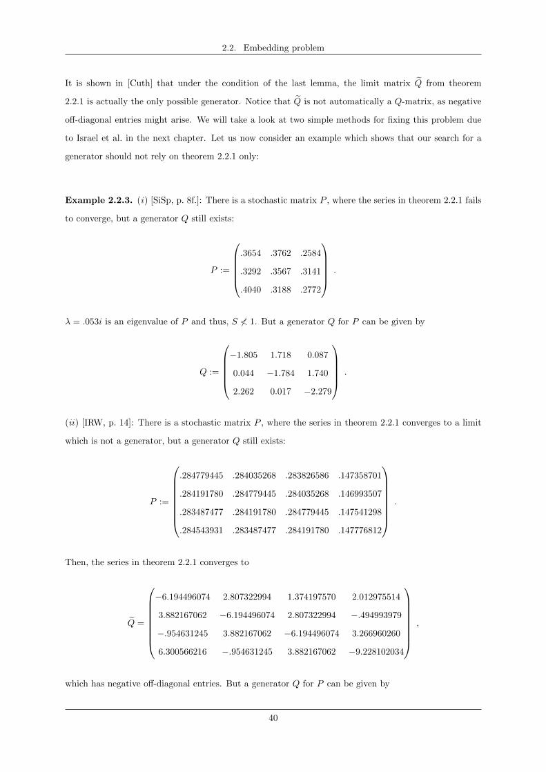
generator should not rely on theorem 2.2.1 only:
Example 2.2.3. (i) [SiSp, p. 8f.]: There is a stochastic matrix P , where the series in theorem 2.2.1 fails
to converge, but a generator Q still exists:
P :=
.3654 .3762 .2584
.3292 .3567 .3141
.4040 .3188 .2772
.
λ = .053i is an eigenvalue of P and thus, S 6< 1. But a generator Q for P can be given by
Q :=
−1.805 1.718 0.087
0.044 −1.784 1.740
2.262 0.017 −2.279
.
(ii) [IRW, p. 14]: There is a stochastic matrix P , where the series in theorem 2.2.1 converges to a limit
which is not a generator, but a generator Q still exists:
P :=
.284779445 .284035268 .283826586 .147358701
.284191780 .284779445 .284035268 .146993507
.283487477 .284191780 .284779445 .147541298
.284543931 .283487477 .284191780 .147776812
.
Then, the series in theorem 2.2.1 converges to
Q =
−6.194496074 2.807322994 1.374197570 2.012975514
3.882167062 −6.194496074 2.807322994 −.494993979
−.954631245 3.882167062 −6.194496074 3.266960260
6.300566216 −.954631245 3.882167062 −9.228102034
,
which has negative off-diagonal entries. But a generator Q for P can be given by
40
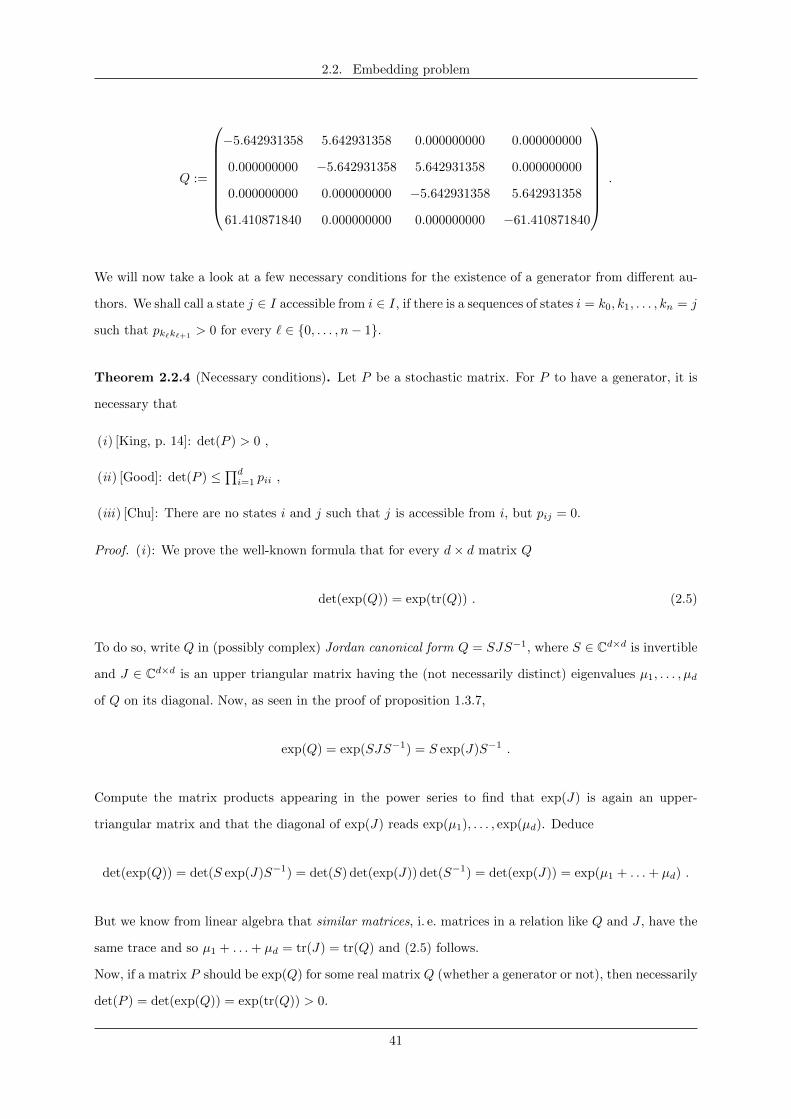
2.2. Embedding problem
Q :=
−5.642931358 5.642931358 0.000000000 0.000000000
0.000000000 −5.642931358 5.642931358 0.000000000
0.000000000 0.000000000 −5.642931358 5.642931358
61.410871840 0.000000000 0.000000000 −61.410871840
.
We will now take a look at a few necessary conditions for the existence of a generator from different au-
thors. We shall call a state j ∈ I accessible from i ∈ I, if there is a sequences of states i = k0, k1, . . . , kn = j
such that pk`k`+1> 0 for every ` ∈ 0, . . . , n− 1.
Theorem 2.2.4 (Necessary conditions). Let P be a stochastic matrix. For P to have a generator, it is
necessary that
(i) [King, p. 14]: det(P ) > 0 ,
(ii) [Good]: det(P ) ≤∏di=1 pii ,
(iii) [Chu]: There are no states i and j such that j is accessible from i, but pij = 0.
Proof. (i): We prove the well-known formula that for every d× d matrix Q
det(exp(Q)) = exp(tr(Q)) . (2.5)
To do so, write Q in (possibly complex) Jordan canonical form Q = SJS−1, where S ∈ Cd×d is invertible
and J ∈ Cd×d is an upper triangular matrix having the (not necessarily distinct) eigenvalues µ1, . . . , µd
of Q on its diagonal. Now, as seen in the proof of proposition 1.3.7,
exp(Q) = exp(SJS−1) = S exp(J)S−1 .
Compute the matrix products appearing in the power series to find that exp(J) is again an upper-
triangular matrix and that the diagonal of exp(J) reads exp(µ1), . . . , exp(µd). Deduce
det(exp(Q)) = det(S exp(J)S−1) = det(S) det(exp(J)) det(S−1) = det(exp(J)) = exp(µ1 + . . .+ µd) .
But we know from linear algebra that similar matrices, i. e. matrices in a relation like Q and J , have the
same trace and so µ1 + . . .+ µd = tr(J) = tr(Q) and (2.5) follows.
Now, if a matrix P should be exp(Q) for some real matrix Q (whether a generator or not), then necessarily
det(P ) = det(exp(Q)) = exp(tr(Q)) > 0.
41
2.2. Embedding problem
(ii): Let P have a generator Q and write P (t) := exp(tQ) for t ≥ 0. We consider the real-valued function
pii(t) := (P (t))ii. This mapping is represented everywhere by a convergent power series, since
pii(t) =
( ∞∑n=0
(tQ)n
n!
)ii
=
∞∑n=0
(Qn)iitn
n!.
Thus, pii(t) is differentiable and we can use term by term differentiation to find
p′ii(t) =
∞∑n=0
(Qn)iintn−1
n!
=
( ∞∑n=1
Qntn−1
(n− 1)!
)ii
=
(Q
∞∑n=1
(tQ)n−1
(n− 1)!
)ii
= (Q exp(tQ))ii .
Since Q has non-negative off-diagonal entries and P (t) = exp(tQ) is a stochastic matrix, for every t ≥ 0
p′ii(t) = (Q exp(tQ))ii =
d∑j=1
qij(P (t))ji ≥ qii(P (t))ii = qiipii(t) .
We follow [Zhao] and deduce
d
dt
(pii(t) exp(−tqii)
)=(p′ii(t)− qiipii(t)
)exp(−tqii) ≥ 0 .
This means that pii(t) exp(−tqii) ≥ pii(0) exp(−0 qii) = 1, which is equivalent to pii(t) ≥ exp(tqii) and
especially implies pii ≥ exp(qii). Thus, using (2.5),
d∏i=1
pii ≥d∏i=1
exp(qii) = exp(tr(Q)) = det(P ) .
(iii): We prove the Levy dichotomy, which states the following: if (pij(t))1≤i,j≤d := P (t) := exp(tQ) with
some generator Q, then for every two states i, j ∈ I we find either pij(t) > 0 ∀ t > 0 or pij(t) = 0 ∀ t > 0.
Assume pij(t) = 0 for some t > 0. Since pjj(s)→ 1 as s→ 0, there has to be s∗ > 0 such that pjj(s) > 0
for every s < s∗. Thus, pij(t/n) > 0 for sufficiently large n ∈ N. Using a generalization of the Cauchy
product theorem, we can show that
exp(A+B) = exp(A) exp(B) (2.6)
for commuting matrices A,B. This gives P (t) = P (t/n)(P (t/n))n−1 and especially pij(t) ≥ pij(t/n) ·
(pjj(t/n))n−1. Hence, pij(t/n) = 0 for all sufficiently large n ∈ N. But a standard result from complex
42
2.2. Embedding problem
analysis says that the zeros of an entire function, like pij(s), can only have an accumulation point (here
0), if the function is identical to zero. This means pij(s) = 0 ∀ s > 0, which proves the assertion.
Let us rephrase part (iii) of the last theorem in a more explicit version due to Israel et al. [IRW, p. 17]:
Lemma 2.2.5 (Quantitative Levy dichotomy). If P has a generator, then the entries of P must satisfy
pij ≥ mmrr(m+ r)−(m+r)d∑k=1
(pik − bm)(pkj − br)1pik>bm,pkj>br
for all positive integers m and r. Here, bm := 1 −∑m`=0 e
−λλ`/`!, which equals the probability that a
Poisson random variable with mean λ := max 1 ≤ i ≤ d(−qii) takes a value greater than m. Additionally,
1A denotes the indicator function of the event A.
Proof. See [IRW, p. 26].
To finish this section, I want to quote a few more existence results by different authors. The proofs can
be found in the respective sources:
Proposition 2.2.6 (Additional results). Let P be a d× d transition matrix.
(i) [Elf]: If any eigenvalues λ 6= 1 of P satisfies |λ| = 1, then no generator for P exists.
(ii) [Elf]: If any negative eigenvalue of P has odd algebraic multiplicity, then no generator for P exists.
(iii) [King, p. 16]: The set of all embeddable matrices is relatively closed inside the set of all matrices
with positive determinant.
(iv) [King, p. 22]: A regular matrix P is embeddable, if and only if for every n ∈ N there exists a
stochastic matrix P1/n such that (P1/n)n = P .
(v) [Runn]: For P to be embeddable, all eigenvalues of P have to lie in D ∪D, where D is the region of
the complex plane bounded by the curve
(exp
(−t+t cos(2π/d)
)cos(t sin(2π/d)
), exp
(−t+t cos(2π/d)
)sin(t sin(2π/d)
))| 0 ≤ t ≤ π/ sin(2π/d)
.
43
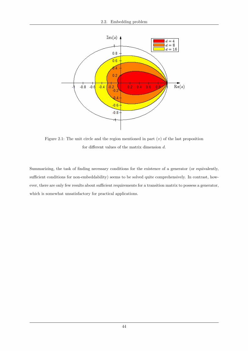
2.2. Embedding problem
Figure 2.1: The unit circle and the region mentioned in part (v) of the last proposition
for different values of the matrix dimension d.
Summarizing, the task of finding necessary conditions for the existence of a generator (or equivalently,
sufficient conditions for non-embeddability) seems to be solved quite comprehensively. In contrast, how-
ever, there are only few results about sufficient requirements for a transition matrix to possess a generator,
which is somewhat unsatisfactory for practical applications.
44
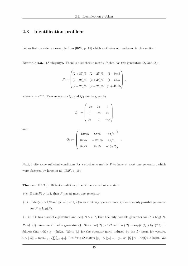
2.3. Identification problem
2.3 Identification problem
Let us first consider an example from [IRW, p. 15] which motivates our endeavor in this section:
Example 2.3.1 (Ambiguity). There is a stochastic matrix P that has two generators Q1 and Q2:
P :=
(2 + 3b)/5 (2− 2b)/5 (1− b)/5
(2− 2b)/5 (2 + 3b)/5 (1− b)/5
(2− 2b)/5 (2− 2b)/5 (1 + 4b)/5
,
where b := e−4π. Two generators Q1 and Q2 can be given by
Q1 :=
−2π 2π 0
0 −2π 2π
4π 0 −4π
and
Q2 :=
−12π/5 8π/5 4π/5
8π/5 −12π/5 4π/5
8π/5 8π/5 −16π/5
.
Next, I cite some sufficient conditions for a stochastic matrix P to have at most one generator, which
were observed by Israel et al. [IRW, p. 16]:
Theorem 2.3.2 (Sufficient conditions). Let P be a stochastic matrix.
(i) : If det(P ) > 1/2, then P has at most one generator.
(ii) : If det(P ) > 1/2 and ‖P−I‖ < 1/2 (in an arbitrary operator norm), then the only possible generator
for P is Log(P ).
(iii) : If P has distinct eigenvalues and det(P ) > e−π, then the only possible generator for P is Log(P ).
Proof. (i): Assume P had a generator Q. Since det(P ) > 1/2 and det(P ) = exp(tr(Q)) by (2.5), it
follows that tr(Q) > − ln(2). Write ‖.‖ for the operator norm induced by the L1 norm for vectors,
i. e. ‖Q‖ = max1≤j≤d∑di=1 |qij |. But for a Q-matrix |qij | ≤ |qii| = −qii, so ‖Q‖ ≤ − tr(Q) < ln(2). We
45

2.3. Identification problem
finish the proof by showing that the matrix exponential is one-to-one on Q ∈ Cd×d | ‖Q‖ < ln(2):
Therefore, let Q1, Q2 be two complex d × d matrices such that ‖Q1‖, ‖Q2‖ < r for some 0 ≤ r < ln(2)
and Q1 6= Q2, which is equivalent to ‖Q1−Q2‖ > 0. Then, using the triangle inequality and the formula
An − Bn =∑n−1k=0 A
k(A − B)Bn−1−k for matrices A,B, which is a generalization of the well-known
identity xn − yn =∑n−1k=0 x
k(x− y)yn−1−k for numbers x, y, deduce
‖ exp(Q1)− exp(Q2)− (Q1 −Q2)‖ ≤∞∑n=2
‖Qn1 −Qn2‖/n!
≤∞∑n=2
n−1∑k=0
‖Qk1(Q1 −Q2)Qn−1−k2 ‖/n!
≤ ‖Q1 −Q2‖∞∑n=2
nrn−1/n!
= ‖Q1 −Q2‖(er − 1) < ‖Q1 −Q2‖ .
This means that exp(Q1)− exp(Q2) 6= 0, which is equivalent to exp(Q1) 6= exp(Q1).
(ii): Let ‖.‖ denote any operator norm such that ‖P − I‖ =: r < 1/2. As a corollary of the spectral
radius formula, S = r(P − I) ≤ ‖P − I‖ = r < 1/2, so the series in theorem 2.2.1 converges. Use the
triangle inequality and the power series expansion of the real logarithm ln in (−1, 1] to deduce
‖Log(P )‖ ≤∞∑n=0
rn/n = −∞∑n=0
(−1)n+1(−r)n/n = − ln(1− r) < ln(2) .
The assertion now follows from the proof of (i).
(iii): Again, assume P had a generator Q. Since P has distinct eigenvalues and Q commutes with
exp(Q) = P , we know from proposition 1.3.7 (iii) that Q has to be g(P ) for some g ∈ H(P ). Use part
(ii) of the same proposition and the composition identity to deduce that g has to satisfy eg(λ) = λ for
every eigenvalue λ of P . This means g(λ) is one of the logarithms of λ for every eigenvalue λ of P .
Since det(P ) > e−π, the complex number 0 can not be an eigenvalue of P and so we know from complex
analysis that there always exists a branch f of the complex logarithm which is holomorphic in an open
neighborhood of σ(P ) and satisfies f(λ) = g(λ) for every λ. This means that Q = g(P ) = f(P ). We will
show that necessarily f = Log: it follows from det(P ) > e−π that 0 ≥ tr(Q) > −π. Write r := − tr(Q).
Now, Q+rI is a matrix that has only non-negative entries. By virtue of proposition 1.3.4 and the spectral
mapping theorem, σ(Q+ rI) = σ(Q) + r. Since Q is a generator, σ(Q)∩ (0,∞) = ∅ and so the maximum
non-negative eigenvalue of Q + rI is r. The well-known Perron-Frobenius theorem now says that the
absolute value of every element of σ(Q+ rI) can not be greater than r. In particular, the imaginary part
of every eigenvalue of Q has to lie in [−r, r]. But Log is the only branch of the complex logarithm, whose
imaginary part lies in (−π, π), so f can only be Log.
46
2.3. Identification problem
Existence and uniqueness of a generator for a stochastic matrix with only real distinct eigenvalues can
be evaluated easily using the following criterion from [IRW, p. 16]:
Proposition 2.3.3 (Real distinct eigenvalues). Let P be a stochastic matrix with only real distinct
eigenvalues.
(i) If all eigenvalues of P are positive, then Log(P ) is the only possible generator for P .
(ii) If P has any negative eigenvalues, then there is no generator for P .
Proof. (i): Suppose Q is a generator for P . First we show that, in this situation, the eigenvalues of Q
have to be real. Since P = exp(Q) has distinct eigenvalues and σ(exp(Q)) = exp(σ(Q)) by virtue of the
spectral mapping theorem, exp is one-to-one on σ(Q). Now, if we assumed an eigenvalue λ ∈ C \R of Q,
then λ 6= λ would also be in σ(Q), because Q is a real matrix. But as the eigenvalues of P = exp(Q) are
real, it would follow that exp(λ) = exp(λ) = exp(λ), which contradicts injectivity of exp on σ(Q).
Since the matrix P has distinct eigenvalues, we know from the proof of the last theorem that Q = f(P ),
where f is some branch of the complex logarithm. Now, the above arguments force f(λ) to be real for
every λ ∈ σ(Q). Thus, the principal branch Log is the only possible candidate for f , so Q = Log(P ).
(ii): If P has any negative eigenvalues, then Log can not be defined in an open neighborhood of σ(Q)
and thus, by virtue of the proof of (i), no generator exists.
The last result due to Israel et al. [IRW, p. 18] is very useful for making an algorithmic approach to
finding generators for continuous-time Markov chains:
Theorem 2.3.4 (Limiting the possible branches). Let P be a stochastic matrix with distinct eigenvalues.
If Q is a generator for P , then every eigenvalue λ of Q satisfies | Im(λ)| ≤ − ln(det(P )) (necessarily
det(P ) > 0 by virtue of theorem 2.2.4 (i)). In particular, only finitely many branches of the complex
logarithm could possibly give rise to a generator for P .
Proof. We follow the proof of theorem 2.3.2 (i) closely. If P has a generator Q, then again exp(tr(Q)) =
det(P ), so tr(Q) = ln(det(P )). Write r := − tr(Q). Then, as argued before, Q + rI is a matrix with
non-negative entries and maximum non-negative eigenvalue r. Deduce with the Perron-Frobenius theorem
that | Im(λ)| ≤ |λ| ≤ r = − ln(det(P )) for every eigenvalue λ of Q.
47
2.3. Identification problem
We draw the conclusion that the identification problem has been solved a bit more gratifyingly in the
literature than the embedding problem of the last section. A lot of easy-to-check sufficient conditions
involving only the determinant of the matrix were found. Necessary requirements for uniqueness of a
generator would have been of no great value, anyway.
48
Chapter 3
Algorithms and numerical examples
3.1 Algorithms to search for a generator
Let us first consider the case where the transition matrix P has distinct eigenvalues. In [IRW, p. 18f.],
the following algorithm to search for a generator in this situation was proposed:
We have argued in the last section that a possible generator for a stochastic matrix P with distinct
eigenvalues can only have the form Q = f(P ), where f is some branch of the complex logarithm which is
analytic in a neighborhood of the spectrum of P . Furthermore, we have discussed that such a function f
has to satisfy f(λj) = ln(rj) + i(θj + 2πkj), where λ1 = r1eiθ1 , . . . , λd = rde
iθd are the eigenvalues of P in
unique polar coordinate representation with rj > 0, θj ∈ (−π, π], j = 1, . . . , d and k1, . . . , kd are integers.
Theorem 2.3.4 gives an additional bound on the imaginary part of the values of f , which ensures that
only finitely many branches need to be considered. Thus, we could simply search for a generator for P
by computing f(P ) for each branch f in question and check, if f(P ) is a generator. But proposition 1.3.7
(ii) tells us that f(P ) = g(P ) for any other function g satisfying f(λ) = g(λ) for every eigenvalue λ of
P . Hence, the possible candidates can be computed more easily using an interpolation polynomial g from
numerical mathematics. The complete algorithm reads as follows:
Algorithm 3.1.1 (Distinct eigenvalues). Let P be a stochastic matrix.
(i) Compute the eigenvalues λ1, . . . , λd of P and validate that they are distinct.
(ii) For each eigenvalue λj = rjeiθj , rj > 0, θj ∈ (−π, π] choose an integer kj , such that f(λj) :=
ln(rj) + i(θj + 2πkj) satisfies | Im(f(λj))| = |θj + 2πkj | ≤ − ln(det(P )).
(iii) Write g for the Lagrange interpolation polynomial for the data points (λ1, f(λ1)), . . . , (λd, f(λd)),
which is given for λ ∈ C by
g(λ) :=
d∑j=1
d∏k=1k 6=j
λ− λkλj − λk
f(λj) .
49
3.1. Algorithms to search for a generator
(iv) Compute the matrix g(P ) for this g and check, if it is a generator for P .
(v) Repeat from (ii) with a different choice for the integers k1, . . . , kd. Continue until all admissible
constellations have been considered.
Remark 3.1.2 (Modifications of the above algorithm). A very similar algorithm to the one presented
above already appeared earlier in [SiSp, pp. 16-19, 25-26]. The only real difference was the bounding result
for the eigenvalues of the generator which was invoked to limit the number of possible branches of the
complex logarithm. As seen above, Israel et al. used theorem 2.3.4, whereas Singer and Spilerman relied
on proposition 2.2.6 (v). [SiSp, pp. 19-25, 26-29] also contains an adaption of the above algorithm to the
case, where the eigenvalues of P are not distinct. The essential idea is to require certain derivatives of
the interpolation polynomial and the branches of the complex logarithm to agree at repeated eigenvalues.
However, since in practice most transition matrices seem to have distinct eigenvalues, this method is not
discussed in more detail here.
If an exact generator could not be found, the following modification techniques from [IRW, p. 6] at least
allows us to determine reasonable approximations based on theorem 2.2.1:
Algorithm 3.1.3 (Non-negativity modifications). Empirically, if negative off-diagonal entries arise in
the matrix Q from theorem 2.2.1, then they will usually be quite small. A naive approach would be to
change all negative off-diagonal entries to zero and adjust the diagonal entries accordingly to ensure that
the new matrix still has row-sums zero. This means, we would modify Q to Q by setting
qij := max(qij , 0), i 6= j; qii := qii +
d∑j=1j 6=i
min(qij , 0) . (3.1)
A more refined method is to distribute the negative excess over the diagonal entry and all non-negative
entries of a row, proportional to their size. We can leave rows that are identical to zero as they are, since
they need no modification. For each other row i we could write
Gi := |qii|+d∑j=1j 6=i
max(qij , 0); Bi :=
d∑j=1j 6=i
min(qij , 0) .
for the ”good” and ”bad” totals and find Gi > 0.
50
3.1. Algorithms to search for a generator
We would then set
qij :=
0, i 6= j and qij < 0
qij −Bi|qij |/Gi, otherwise
. (3.2)
When the diagonal entries of Q have a large absolute and the negative off-diagonal entries remain com-
paratively small, the two modifications will lead to very similar results.
The next algorithm is taken from [JLT, p. 504f.]. It was deduced in an economic model of greater scope
with an underlying assumption that the probability of a debtor’s credit rating changing more than once
in a year is negligible.
Algorithm 3.1.4 (Explicit construction). Let P be a d × dtransition matrix. For i = 1, . . . , d − 1 and
j = 1, . . . , d set
qii := ln(pii); qij := pij ln(pii)/(pii − 1), i 6= j . (3.3)
Treat the case i = d by qdj := 0 for j = 1, . . . , d.
To finish this section, we take a look at a simple rule from [IRW, p. 15], which allows substantiated choice
of a generator, if there are multiple options:
Algorithm 3.1.5 (Selection rule). If a stochastic matrix P possesses multiple generators, then choose
the one which minimizes the quantity
J =
d∑i,j=1
|i− j| qij
This way, you ensure that jumping to a remote rating is not too likely, which is adequate for credit
transition matrices.
51
3.2. Numerical examples
3.2 Numerical examples
Let us now try to apply the developed theory to some real examples. It has to be said in advance that,
up to today, this unfortunately does not work as expected for credit rating transition matrices. This is
due to the fact that, so far, such matrices never pass the test of the Levy dichotomy. Hence, an exact
generator will never exist and most of the results become obsolete. If we consider the developments of
rating transition matrices until today, we can at least hope that with an increasing number of observa-
tions, this problem could disappear. Also, the situation might already be more favorable these days in
other fields of research, where Markov chain models are used.
In the following, let us ”at least” try to find approximate generators for some real credit rating matri-
ces. We will have to make up more or less heuristic rules and hypotheses to guide our search. Despite
the adverse circumstances, we shall try to investigate, if one of the methods from the previous section is
superior to the others and, if there are factors in the underlying data which influence the outcome notably.
Example 3.2.1 (Standard & Poor’s 1981-2013). Our starting point shall be the average annual transition
matrix for the years 1981− 2013 provided by the credit rating agency ”Standard & Poor’s” in their 2013
corporate default and rating transition study [SnP1]. We reallocate the share of the transitions to the
status ”Not rated” using the intuitive equation (31) from [JLT, p. 506]. A representation of the resulting
matrix P with four decimal places reads
P ≈
0.9004 0.0918 0.0055 0.0005 0.0008 0.0003 0.0005 0.0000
0.0057 0.9006 0.0861 0.0058 0.0006 0.0007 0.0002 0.0002
0.0003 0.0196 0.9164 0.0575 0.0037 0.0015 0.0002 0.0007
0.0001 0.0013 0.0383 0.9096 0.0408 0.0063 0.0014 0.0022
0.0002 0.0004 0.0017 0.0576 0.8451 0.0786 0.0076 0.0089
0.0000 0.0003 0.0012 0.0025 0.0621 0.8368 0.0505 0.0465
0.0000 0.0000 0.0018 0.0027 0.0081 0.1583 0.5140 0.3152
0.0000 0.0000 0.0000 0.0000 0.0000 0.0000 0.0000 1.0000
.
The eight rows and columns represent, in order, the credit ratings AAA, AA, A, BBB, BB, B, CCC/C
and Default. As already announced, P does not satisfy the Levy Dichotomy so an exact generator does
not exist. We observe that the eigenvalues of P are distinct and positive, so proposition 2.3.3 (i) would
have ruled out all branches of the complex logarithm but the principal one for our search anyway.
52
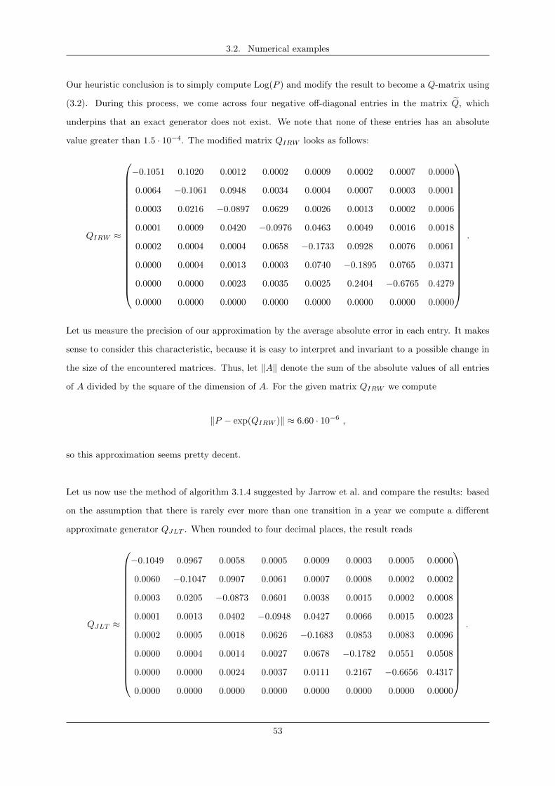
3.2. Numerical examples
Our heuristic conclusion is to simply compute Log(P ) and modify the result to become a Q-matrix using
(3.2). During this process, we come across four negative off-diagonal entries in the matrix Q, which
underpins that an exact generator does not exist. We note that none of these entries has an absolute
value greater than 1.5 · 10−4. The modified matrix QIRW looks as follows:
QIRW ≈
−0.1051 0.1020 0.0012 0.0002 0.0009 0.0002 0.0007 0.0000
0.0064 −0.1061 0.0948 0.0034 0.0004 0.0007 0.0003 0.0001
0.0003 0.0216 −0.0897 0.0629 0.0026 0.0013 0.0002 0.0006
0.0001 0.0009 0.0420 −0.0976 0.0463 0.0049 0.0016 0.0018
0.0002 0.0004 0.0004 0.0658 −0.1733 0.0928 0.0076 0.0061
0.0000 0.0004 0.0013 0.0003 0.0740 −0.1895 0.0765 0.0371
0.0000 0.0000 0.0023 0.0035 0.0025 0.2404 −0.6765 0.4279
0.0000 0.0000 0.0000 0.0000 0.0000 0.0000 0.0000 0.0000
.
Let us measure the precision of our approximation by the average absolute error in each entry. It makes
sense to consider this characteristic, because it is easy to interpret and invariant to a possible change in
the size of the encountered matrices. Thus, let ‖A‖ denote the sum of the absolute values of all entries
of A divided by the square of the dimension of A. For the given matrix QIRW we compute
‖P − exp(QIRW )‖ ≈ 6.60 · 10−6 ,
so this approximation seems pretty decent.
Let us now use the method of algorithm 3.1.4 suggested by Jarrow et al. and compare the results: based
on the assumption that there is rarely ever more than one transition in a year we compute a different
approximate generator QJLT . When rounded to four decimal places, the result reads
QJLT ≈
−0.1049 0.0967 0.0058 0.0005 0.0009 0.0003 0.0005 0.0000
0.0060 −0.1047 0.0907 0.0061 0.0007 0.0008 0.0002 0.0002
0.0003 0.0205 −0.0873 0.0601 0.0038 0.0015 0.0002 0.0008
0.0001 0.0013 0.0402 −0.0948 0.0427 0.0066 0.0015 0.0023
0.0002 0.0005 0.0018 0.0626 −0.1683 0.0853 0.0083 0.0096
0.0000 0.0004 0.0014 0.0027 0.0678 −0.1782 0.0551 0.0508
0.0000 0.0000 0.0024 0.0037 0.0111 0.2167 −0.6656 0.4317
0.0000 0.0000 0.0000 0.0000 0.0000 0.0000 0.0000 0.0000
.
53
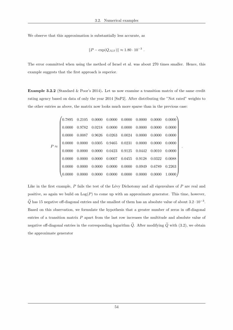
3.2. Numerical examples
We observe that this approximation is substantially less accurate, as
‖P − exp(QJLT )‖ ≈ 1.80 · 10−3 .
The error committed when using the method of Israel et al. was about 270 times smaller. Hence, this
example suggests that the first approach is superior.
Example 3.2.2 (Standard & Poor’s 2014). Let us now examine a transition matrix of the same credit
rating agency based on data of only the year 2014 [SnP2]. After distributing the ”Not rated” weights to
the other entries as above, the matrix now looks much more sparse than in the previous case:
P ≈
0.7895 0.2105 0.0000 0.0000 0.0000 0.0000 0.0000 0.0000
0.0000 0.9782 0.0218 0.0000 0.0000 0.0000 0.0000 0.0000
0.0000 0.0087 0.9626 0.0263 0.0024 0.0000 0.0000 0.0000
0.0000 0.0000 0.0305 0.9465 0.0231 0.0000 0.0000 0.0000
0.0000 0.0000 0.0000 0.0423 0.9125 0.0442 0.0010 0.0000
0.0000 0.0000 0.0000 0.0007 0.0455 0.9128 0.0322 0.0088
0.0000 0.0000 0.0000 0.0000 0.0000 0.0949 0.6789 0.2263
0.0000 0.0000 0.0000 0.0000 0.0000 0.0000 0.0000 1.0000
.
Like in the first example, P fails the test of the Levy Dichotomy and all eigenvalues of P are real and
positive, so again we build on Log(P ) to come up with an approximate generator. This time, however,
Q has 15 negative off-diagonal entries and the smallest of them has an absolute value of about 3.2 · 10−3.
Based on this observation, we formulate the hypothesis that a greater number of zeros in off-diagonal
entries of a transition matrix P apart from the last row increases the multitude and absolute value of
negative off-diagonal entries in the corresponding logarithm Q. After modifying Q with (3.2), we obtain
the approximate generator
54
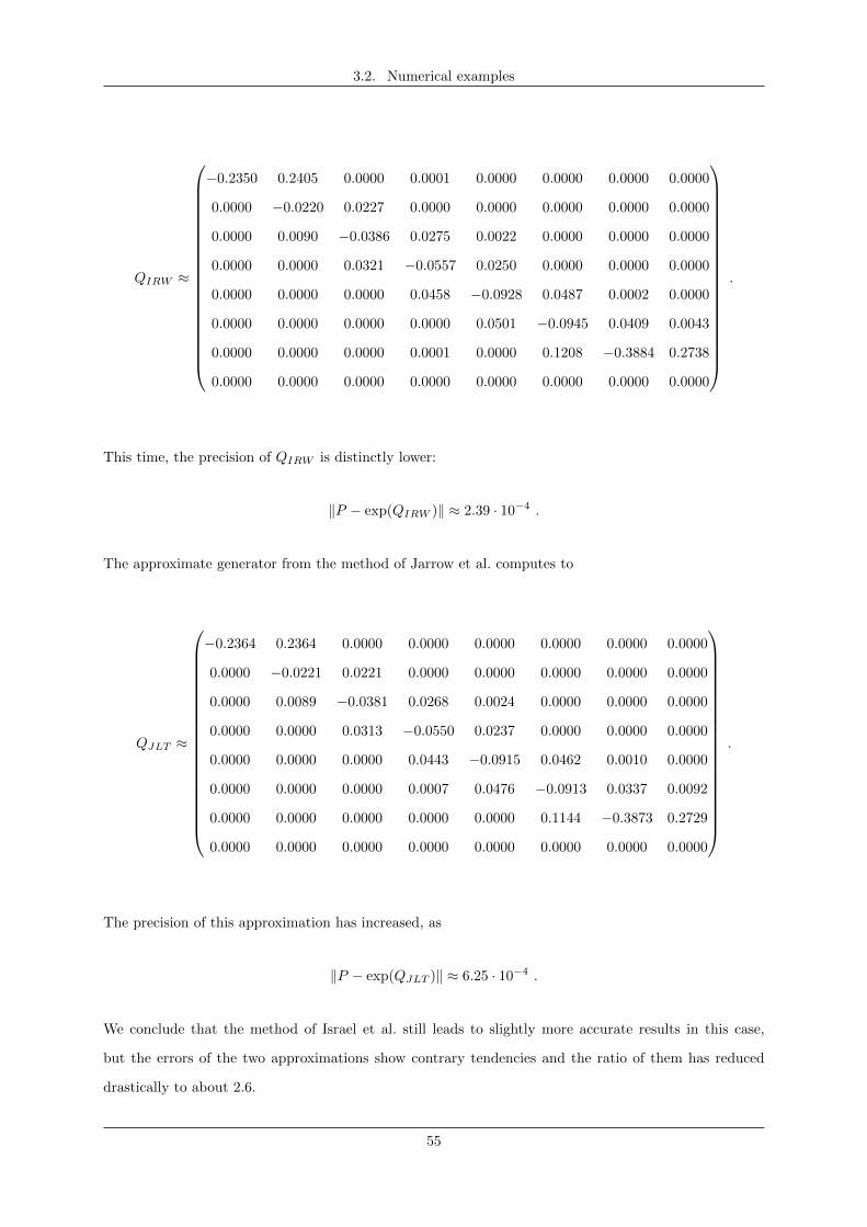
3.2. Numerical examples
QIRW ≈
−0.2350 0.2405 0.0000 0.0001 0.0000 0.0000 0.0000 0.0000
0.0000 −0.0220 0.0227 0.0000 0.0000 0.0000 0.0000 0.0000
0.0000 0.0090 −0.0386 0.0275 0.0022 0.0000 0.0000 0.0000
0.0000 0.0000 0.0321 −0.0557 0.0250 0.0000 0.0000 0.0000
0.0000 0.0000 0.0000 0.0458 −0.0928 0.0487 0.0002 0.0000
0.0000 0.0000 0.0000 0.0000 0.0501 −0.0945 0.0409 0.0043
0.0000 0.0000 0.0000 0.0001 0.0000 0.1208 −0.3884 0.2738
0.0000 0.0000 0.0000 0.0000 0.0000 0.0000 0.0000 0.0000
.
This time, the precision of QIRW is distinctly lower:
‖P − exp(QIRW )‖ ≈ 2.39 · 10−4 .
The approximate generator from the method of Jarrow et al. computes to
QJLT ≈
−0.2364 0.2364 0.0000 0.0000 0.0000 0.0000 0.0000 0.0000
0.0000 −0.0221 0.0221 0.0000 0.0000 0.0000 0.0000 0.0000
0.0000 0.0089 −0.0381 0.0268 0.0024 0.0000 0.0000 0.0000
0.0000 0.0000 0.0313 −0.0550 0.0237 0.0000 0.0000 0.0000
0.0000 0.0000 0.0000 0.0443 −0.0915 0.0462 0.0010 0.0000
0.0000 0.0000 0.0000 0.0007 0.0476 −0.0913 0.0337 0.0092
0.0000 0.0000 0.0000 0.0000 0.0000 0.1144 −0.3873 0.2729
0.0000 0.0000 0.0000 0.0000 0.0000 0.0000 0.0000 0.0000
.
The precision of this approximation has increased, as
‖P − exp(QJLT )‖ ≈ 6.25 · 10−4 .
We conclude that the method of Israel et al. still leads to slightly more accurate results in this case,
but the errors of the two approximations show contrary tendencies and the ratio of them has reduced
drastically to about 2.6.
55
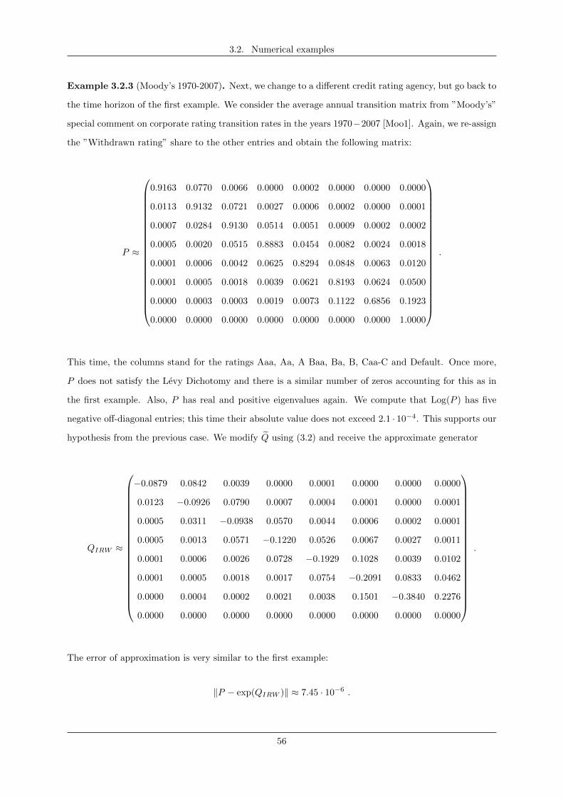
3.2. Numerical examples
Example 3.2.3 (Moody’s 1970-2007). Next, we change to a different credit rating agency, but go back to
the time horizon of the first example. We consider the average annual transition matrix from ”Moody’s”
special comment on corporate rating transition rates in the years 1970−2007 [Moo1]. Again, we re-assign
the ”Withdrawn rating” share to the other entries and obtain the following matrix:
P ≈
0.9163 0.0770 0.0066 0.0000 0.0002 0.0000 0.0000 0.0000
0.0113 0.9132 0.0721 0.0027 0.0006 0.0002 0.0000 0.0001
0.0007 0.0284 0.9130 0.0514 0.0051 0.0009 0.0002 0.0002
0.0005 0.0020 0.0515 0.8883 0.0454 0.0082 0.0024 0.0018
0.0001 0.0006 0.0042 0.0625 0.8294 0.0848 0.0063 0.0120
0.0001 0.0005 0.0018 0.0039 0.0621 0.8193 0.0624 0.0500
0.0000 0.0003 0.0003 0.0019 0.0073 0.1122 0.6856 0.1923
0.0000 0.0000 0.0000 0.0000 0.0000 0.0000 0.0000 1.0000
.
This time, the columns stand for the ratings Aaa, Aa, A Baa, Ba, B, Caa-C and Default. Once more,
P does not satisfy the Levy Dichotomy and there is a similar number of zeros accounting for this as in
the first example. Also, P has real and positive eigenvalues again. We compute that Log(P ) has five
negative off-diagonal entries; this time their absolute value does not exceed 2.1 · 10−4. This supports our
hypothesis from the previous case. We modify Q using (3.2) and receive the approximate generator
QIRW ≈
−0.0879 0.0842 0.0039 0.0000 0.0001 0.0000 0.0000 0.0000
0.0123 −0.0926 0.0790 0.0007 0.0004 0.0001 0.0000 0.0001
0.0005 0.0311 −0.0938 0.0570 0.0044 0.0006 0.0002 0.0001
0.0005 0.0013 0.0571 −0.1220 0.0526 0.0067 0.0027 0.0011
0.0001 0.0006 0.0026 0.0728 −0.1929 0.1028 0.0039 0.0102
0.0001 0.0005 0.0018 0.0017 0.0754 −0.2091 0.0833 0.0462
0.0000 0.0004 0.0002 0.0021 0.0038 0.1501 −0.3840 0.2276
0.0000 0.0000 0.0000 0.0000 0.0000 0.0000 0.0000 0.0000
.
The error of approximation is very similar to the first example:
‖P − exp(QIRW )‖ ≈ 7.45 · 10−6 .
56
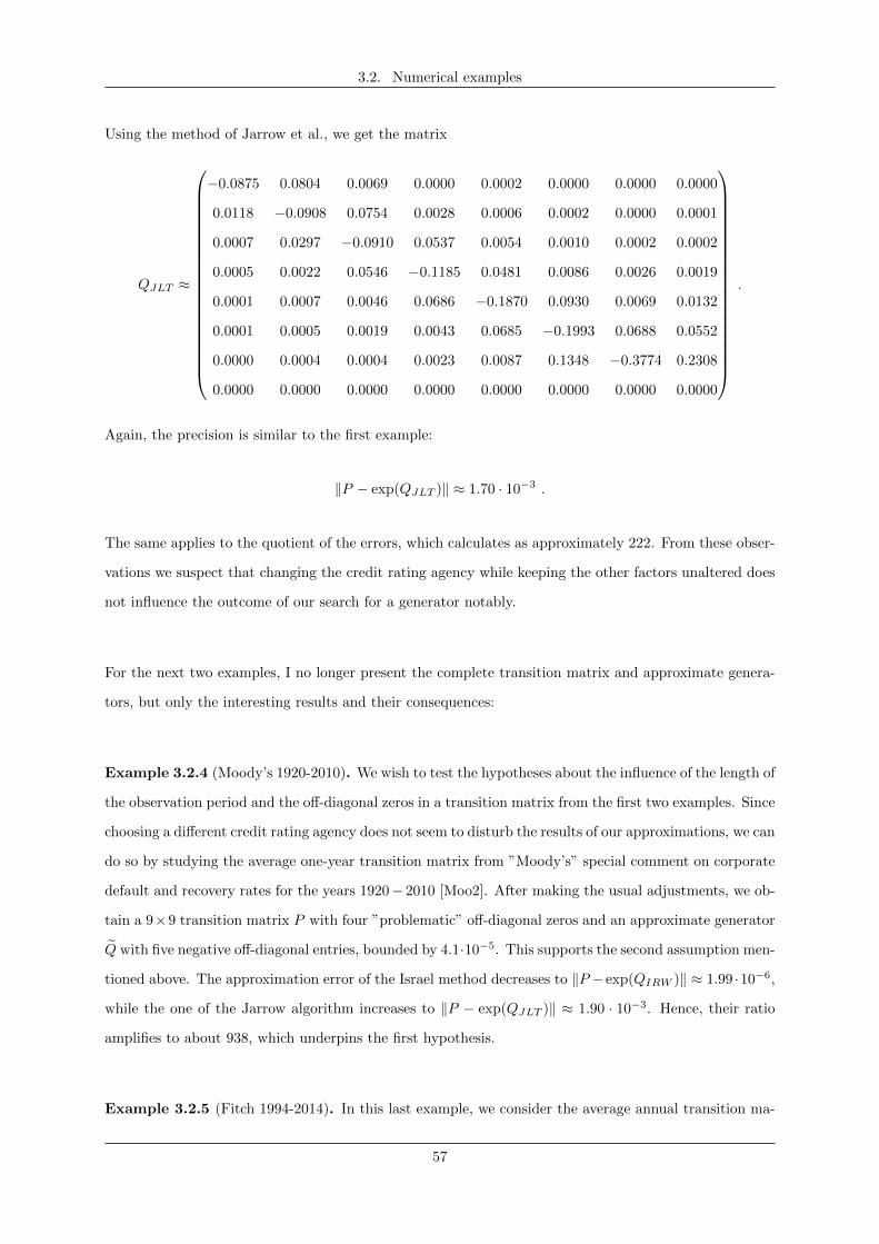
3.2. Numerical examples
Using the method of Jarrow et al., we get the matrix
QJLT ≈
−0.0875 0.0804 0.0069 0.0000 0.0002 0.0000 0.0000 0.0000
0.0118 −0.0908 0.0754 0.0028 0.0006 0.0002 0.0000 0.0001
0.0007 0.0297 −0.0910 0.0537 0.0054 0.0010 0.0002 0.0002
0.0005 0.0022 0.0546 −0.1185 0.0481 0.0086 0.0026 0.0019
0.0001 0.0007 0.0046 0.0686 −0.1870 0.0930 0.0069 0.0132
0.0001 0.0005 0.0019 0.0043 0.0685 −0.1993 0.0688 0.0552
0.0000 0.0004 0.0004 0.0023 0.0087 0.1348 −0.3774 0.2308
0.0000 0.0000 0.0000 0.0000 0.0000 0.0000 0.0000 0.0000
.
Again, the precision is similar to the first example:
‖P − exp(QJLT )‖ ≈ 1.70 · 10−3 .
The same applies to the quotient of the errors, which calculates as approximately 222. From these obser-
vations we suspect that changing the credit rating agency while keeping the other factors unaltered does
not influence the outcome of our search for a generator notably.
For the next two examples, I no longer present the complete transition matrix and approximate genera-
tors, but only the interesting results and their consequences:
Example 3.2.4 (Moody’s 1920-2010). We wish to test the hypotheses about the influence of the length of
the observation period and the off-diagonal zeros in a transition matrix from the first two examples. Since
choosing a different credit rating agency does not seem to disturb the results of our approximations, we can
do so by studying the average one-year transition matrix from ”Moody’s” special comment on corporate
default and recovery rates for the years 1920− 2010 [Moo2]. After making the usual adjustments, we ob-
tain a 9×9 transition matrix P with four ”problematic” off-diagonal zeros and an approximate generator
Q with five negative off-diagonal entries, bounded by 4.1·10−5. This supports the second assumption men-
tioned above. The approximation error of the Israel method decreases to ‖P −exp(QIRW )‖ ≈ 1.99 ·10−6,
while the one of the Jarrow algorithm increases to ‖P − exp(QJLT )‖ ≈ 1.90 · 10−3. Hence, their ratio
amplifies to about 938, which underpins the first hypothesis.
Example 3.2.5 (Fitch 1994-2014). In this last example, we consider the average annual transition ma-
57
3.2. Numerical examples
trix for the years 1994− 2014 from the 2014 global corporate finance transition and default study by the
credit rating agency ”Fitch” [Fit]. Here, the ratings are finely subdivided into 18 categories, giving a much
larger transition matrix than in all the previous examples. Additionally, for the first time, eigenvalues in
C \ R occur and π < − ln(det(P )) ≈ 7.80 < 3π, so hypothetically we can no longer rely on the principal
branch Log of the complex logarithm for our search only. Nevertheless, the results of our investigation are
not very different from the previous examples. We consider both adding and subtracting 2πi in the loga-
rithms of the six eigenvalues in C \R, in all 36 possible constellations. Out of all approximate generators
arising from these combinations, Log(P ) is still the most precise one. Due to the extensive computation
time needed, I was not able to test all 318 variations of allowing a modification in the logarithms of every
eigenvalue, also the real ones. I can only suspect that this would not have changed the outcome. The
approximation errors amount to ‖P − exp(QIRW )‖ ≈ 9.83 · 10−5 and ‖P − exp(QJLT )‖ ≈ 3.30 · 10−3 and
their ratio is about 34, which matches our hypothesis about the influence of the observation period length.
Conclusion 3.2.6. Since the five examples in this section all contribute to a considerably harmonic
overall picture, I dare to make some tentative conclusions: in practice, it seems to work best to simply
compute Log(P ) for a transition matrix and then modify the result to become a Q-matrix. This can
be realized efficiently using interpolation polynomials as suggested by Israel. Applying the logarithm
directly to the diagonal matrix in a Jordan decomposition takes much longer run time and is said to be
numerically unstable. The negative off-diagonal entries in Q always stayed comparatively small and I
would regard the average approximation error in each entry as tolerable. We could observe the tendency
that the two methods seem to react contrarily to an increase in the length of the observation period.
This could be due to Jarrow’s assumption that there rarely ever is more than one transition per year,
which perhaps is not applicable to the real credit rating process and causes even stronger discrepancies
in the long run. Furthermore, the minimum approximation error was larger for more sparse matrices,
which could be interpreted as meaning that the represented processes are less typically Markovian in the
sense of the Levy dichotomy. I also remark that I consider the idea of modifying a transition matrix
beforehand to avoid this problem mentioned in [IRW, p. 20] unfavorable. One would have to make
arbitrary judgments concerning which value the zeros on the off-diagonal should be raised to. I have
tested that making only slight modifications in these entries (of the order 10−4), still did not make any
of the transition matrices embeddable (recall that the Levy dichotomy is only a necessary condition for
the existence of a generator). But altering the values of the problematic entries any greater, would be
all the more discretionary. Lastly, I comment that it might be possible to find a rule for reallocating the
”Not rated” weights which does more justice to the real credit rating process than Jarrow’s guideline, if
one analyzed, what are typically the reasons for such a transition to happen.
58

Bibliography
[Bals] Balser, W. (2010): Vorlesungsmanuskript zur Funktionentheorie; retrieved September 28,
2015 from
http://www.mathematik.uni-ulm.de/m5/balser/Skripten/Funktionentheorie-Master.pdf
[Berg] Berg, C. (2012): Complex Analysis, p. 40f.; retrieved September 28, 2015 from
http://www.math.ku.dk/noter/filer/koman-12.pdf
[Born] Bornemann, F. (2013): Funktionentheorie, Springer Basel
[Chu] Chung, K. L. (1967): Markov chains with stationary transition probabilities, Springer New York
[Cuth] Cuthbert, J. R. (1972): On uniqueness of the logarithm for Markov semi-groups. J. London Math-
ematical Society 4, p. 629
[deBo] de Boor, C. (2013): Linear Algebra, p. 171f.; retrieved September 28, 2015 from
http://pages.cs.wisc.edu/~deboor/443/book.pdf
[Down] Down, A. (2005): Winding Number ; retrived September 28, 2015 from
http://people.duke.edu/~ad159/files/m185/11.pdf
[Elf] Elfving, G. (1937): Zur Theorie der Markoffschen Ketten, Acta Social Science Fennicae n., series
A.2, no. 8, 1-17
[Fit] Fitch Ratings (2015): Global Corporate Finance 2014 Transition and Default Study, p. 23; retrieved
September 28, 2015 from
https://www.fitchratings.com/web_content/nrsro/nav/NRSRO_Exhibit-1.pdf
[Garr] Garrett, P. (2014): Examples of operators and spectra, p. 1f.; retrieved September 28, 2015 from
http://www.math.umn.edu/~garrett/m/fun/notes_2012-13/06b_examples_spectra.pdf
[Good] Goodman, G. S. (1970): An intrinsic time for non-stationary finite Markov chains, Zeitschrift
fur Wahrscheinlichkeitstheorie 16, pp. 165-180
[IRW] Israel, R. B.; Rosenthal, J. S.; Wei, J. Z. (2000): Finding Generators for Markov Chains via Em-
pirical Transition Matrices, with Applications to Credit Ratings
[JLT] Jarrow, R. A.; Lando, D.; Turnbull, S. M. (1997): A Markov model for the term structure of credit
risk spreads, Review of Financial Studies 10, pp. 481-523. ; retrieved September 28, 2015 from
59
Bibliography
http://forum.johnson.cornell.edu/faculty/jarrow/055%20Markov%20Model%20Credit%
20Risk%20RFS%201997.pdf
[King] Kingman, J. F. C. (1962): The imbedding problem for finite Markov chains, Zeitschrift fur
Wahrscheinlichkeitstheorie 1
[Moo1] Moody’s Investor Services (2008): Corporate One-to-Five-Year Rating Transition Rates, p. 2;
retrieved September 28, 2015 from
https://www.moodys.com/sites/products/DefaultResearch/2007100000486361.pdf
[Moo2] Moody’s Inverstor Services (2011): Corporate Default and Recovery Rates, 1920-2010, p. 23;
retrieved September 28, 2015 from
http://efinance.org.cn/cn/FEben/Corporate%20Default%20and%20Recovery%20Rates,
1920-2010.pdf
[Neun] Neuner, C. (2010): Der Riesz-Dunford’sche Funktionalkalkul ; retrieved September 28, 2015 from
http://www.asc.tuwien.ac.at/~funkana/downloads_general/sem_neuner.pdf
[Norr] Norris, J. R. (1998): Markov chains, Cambridge University Press, pp. 1-105
[Rud] Rudin, W. (1991): Functional Analysis, McGraw-Hill Singapore, second edition, p. 253ff.
[Runn] Runnenberg, J. Th. (1962): On Elfving’s problem of imbedding a time-discrete Markov chain in
a continuous time one for finitely many states, Proceedings, Koninklijke Nederlandse Akademie van
Wetenschappen 28 series A, Mathematical Sciences 65 (5), pp. 536-541
[Schn] Schnaubelt, R. (2012): Lecture notes spectral theory, p. 77ff.; retrieved September 28, 2015 from
http://www.math.kit.edu/iana3/~schnaubelt/media/st-skript.pdf
[SiSp] Singer, B.; Spilerman, S. (1976): The Representation of Social Processes by Markov Models; re-
trieved September 28, 2015 from
http://www.stat.cmu.edu/~fienberg/Stat36-835/SingerSpilerman-AJS-1976.pdf
[SnP1] Standard & Poor’s Financial Services (2014): Default, Transition, and Recovery: 2013 Annual
Global Corporate Default Study And Rating Transitions, p. 52; retrieved September 28, 2015 from
http://www.maalot.co.il/publications/fts20140324161422.pdf
[SnP2] Standard & Poor’s Financial Services (2015): Default, Transition, and Recovery: 2014 Annual
Global Corporate Default Study And Rating Transitions, p. 51; retrieved September 28, 2015 from
http://www.nact.org/resources/2014_SP_Global_Corporate_Default_Study.pdf
60
Bibliography
[Swan] Swanson, H. (2015): Why isn’t every element of the spectrum an eigenvalue? (Where is the error
in my proof?); retrieved September 28, 2015 from
http://math.stackexchange.com/questions/1373884/why-isnt-every-element-of-the-\
spectrum-an-eigenvalue-where-is-the-error-in-my
[Tayl] Taylor, M. (year unknown): Banach algebras - Bare Bones Basics, p. 24; retrieved September 28,
2015 from
http://www.unc.edu/math/Faculty/met/banalg.pdf
[Zhao] Zhao, M. (2011): The Gronwall’s Inequality, p. 1; retrieved September 28, 2015 from
http://www.math.ubc.ca/~mingfeng/Talks%20and%20Notes/The%20Gronwall’s%
20inequality.pdf
61

List of Figures
[1] Coat of arms of the Philipps-University Marburg on the title page: retrieved September 28, 2015 from
http://www.online.uni-marburg.de/hrz/stadt/bilder/philtra.gif
62

Declaration
I hereby declare that I have written this bachelor thesis completely on my own and that I have not used
any other sources than the ones listed in the bibliography to do so. This bachelor thesis was not used in
the same or a similar version to achieve an academic grading or is being published elsewhere.
Marburg, September 28, 2015
(Leon Roschig, author)
63


![Option Pricing Under a Discrete-Time Markov Switching ... · arXiv:2006.15054v1 [q-fin.PR] 26 Jun 2020 Option Pricing Under a Discrete-Time Markov Switching Stochastic Volatility](https://img.dokumen.tips/doc/110x75/5fc5bcca12dd631bfe463aea/option-pricing-under-a-discrete-time-markov-switching-arxiv200615054v1-q-finpr.jpg)