Markov Chains: Introductionstat455/lecturenotes/set2.pdf · 72 9. MARKOV CHAINS: INTRODUCTION Markov Chains: A discrete-time stochastic process Xis said to be a Markov Chain if it

9

Markov Chains: Introduction

We now start looking at the material in Chapter 4 of the text. As we

go through Chapter 4 we’ll be more rigorous with some of the theory

that is presented either in an intuitive fashion or simply without proof

in the text.

Our focus is on a class of discrete-time stochastic processes. Recall

that a discrete-time stochastic process is a sequence of random vari-

ables X = {Xn : n ∈ I}, where I is a discrete index set. Unless

otherwise stated, we’ll take the index set I to be the set of nonnegative

integers I = {0, 1, 2, . . .}, so

X = {Xn : n = 0, 1, 2, . . .}.

We’ll denote the state space of X by S (recall that the state space

is the set of all possible values of any of the Xi’s). The state space

is also assumed to be discrete (but otherwise general), and we let |S|denote the number of elements in S (called the cardinality of S). So

|S| could be ∞ or some finite positive integer.

We’ll start by looking at some of the basic structure of Markov chains.

71

72 9. MARKOV CHAINS: INTRODUCTION

Markov Chains:

A discrete-time stochastic process X is said to be a Markov Chain if

it has the Markov Property:

Markov Property (version 1):

For any s, i0, . . . , in−1 ∈ S and any n ≥ 1,

P (Xn = s|X0 = i0, . . . , Xn−1 = in−1) = P (Xn = s|Xn−1 = in−1).

In words, we say that the distribution of Xn given the entire past of

the process only depends on the immediate past. Note that we are not

saying that, for example X10 and X1 are independent. They are not.

However, given X9, for example, X10 is conditionally independent of

X1. Graphically, we may imagine being on a particle jumping around in

the state space as time goes on to form a (random) sample path. The

Markov property is that the distribution of where I go to next depends

only on where I am now, not on where I’ve been. This property is a

reasonable assumption for many (though certainly not all) real-world

processes. Here are a couple of examples.

Example: Suppose we check our inventory once a week and replen-

ish if necessary according to some schedule which depends on the level

of the stock when we check it. Let Xn be the level of the stock at the

beginning of week n. The Markov property for the sequence {Xn}should be reasonable if it is reasonable that the distribution of the

(random) stock level at the beginning of the following week depends

on the stock level now (and the replenishing rule, which we assume

depends only on the current stock level), but not on the stock level

from previous weeks. This assumption would be true if it were true

that demands for the stock for the coming week do not depend on the

past stock levels. �

73

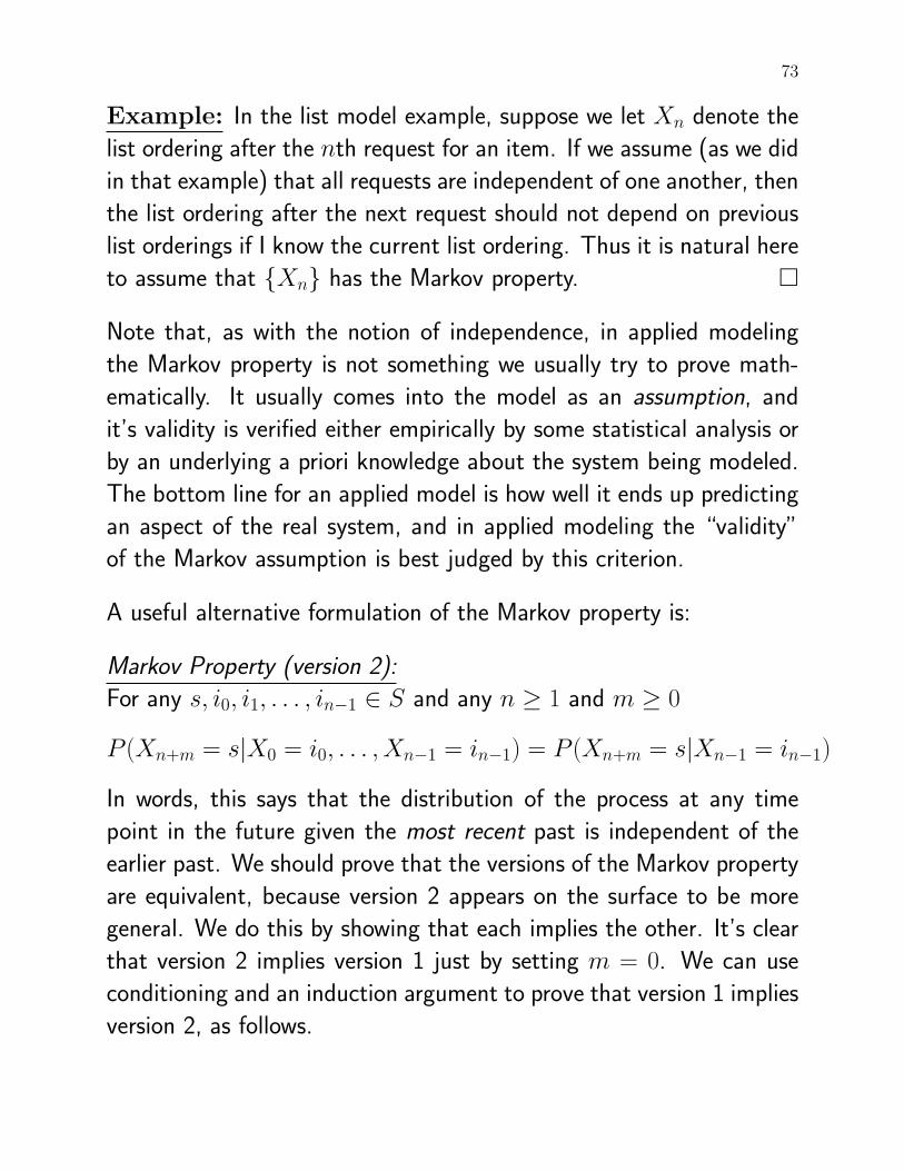
Example: In the list model example, suppose we let Xn denote the

list ordering after the nth request for an item. If we assume (as we did

in that example) that all requests are independent of one another, then

the list ordering after the next request should not depend on previous

list orderings if I know the current list ordering. Thus it is natural here

to assume that {Xn} has the Markov property. �

Note that, as with the notion of independence, in applied modeling

the Markov property is not something we usually try to prove math-

ematically. It usually comes into the model as an assumption, and

it’s validity is verified either empirically by some statistical analysis or

by an underlying a priori knowledge about the system being modeled.

The bottom line for an applied model is how well it ends up predicting

an aspect of the real system, and in applied modeling the “validity”

of the Markov assumption is best judged by this criterion.

A useful alternative formulation of the Markov property is:

Markov Property (version 2):

For any s, i0, i1, . . . , in−1 ∈ S and any n ≥ 1 and m ≥ 0

P (Xn+m = s|X0 = i0, . . . , Xn−1 = in−1) = P (Xn+m = s|Xn−1 = in−1)

In words, this says that the distribution of the process at any time

point in the future given the most recent past is independent of the

earlier past. We should prove that the versions of the Markov property

are equivalent, because version 2 appears on the surface to be more

general. We do this by showing that each implies the other. It’s clear

that version 2 implies version 1 just by setting m = 0. We can use

conditioning and an induction argument to prove that version 1 implies

version 2, as follows.


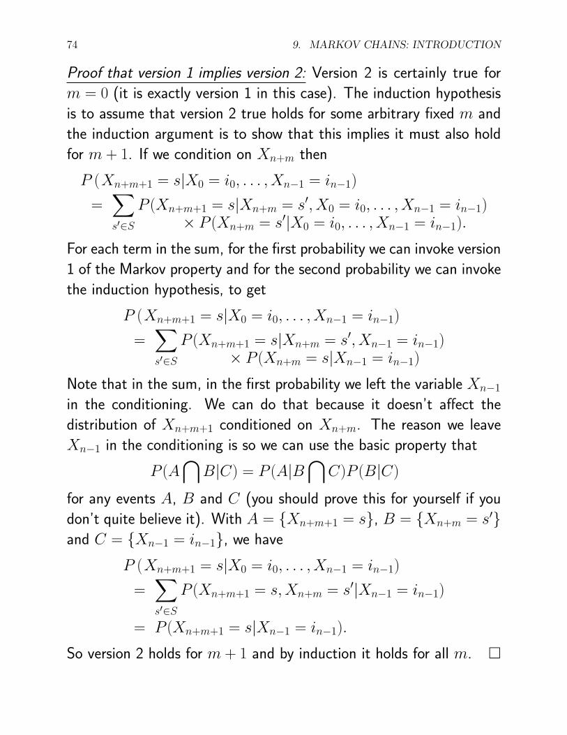
Proof that version 1 implies version 2: Version 2 is certainly true for

m = 0 (it is exactly version 1 in this case). The induction hypothesis

is to assume that version 2 true holds for some arbitrary fixed m and

the induction argument is to show that this implies it must also hold

for m + 1. If we condition on Xn+m then

P (Xn+m+1 = s|X0 = i0, . . . , Xn−1 = in−1)

=∑s′∈S

P (Xn+m+1 = s|Xn+m = s′, X0 = i0, . . . , Xn−1 = in−1)× P (Xn+m = s′|X0 = i0, . . . , Xn−1 = in−1).

For each term in the sum, for the first probability we can invoke version

1 of the Markov property and for the second probability we can invoke

the induction hypothesis, to get

P (Xn+m+1 = s|X0 = i0, . . . , Xn−1 = in−1)

=∑s′∈S

P (Xn+m+1 = s|Xn+m = s′, Xn−1 = in−1)× P (Xn+m = s|Xn−1 = in−1)

Note that in the sum, in the first probability we left the variable Xn−1

in the conditioning. We can do that because it doesn’t affect the

distribution of Xn+m+1 conditioned on Xn+m. The reason we leave

Xn−1 in the conditioning is so we can use the basic property that

P (A⋂

B|C) = P (A|B⋂

C)P (B|C)

for any events A, B and C (you should prove this for yourself if you

don’t quite believe it). With A = {Xn+m+1 = s}, B = {Xn+m = s′}and C = {Xn−1 = in−1}, we have

P (Xn+m+1 = s|X0 = i0, . . . , Xn−1 = in−1)

=∑s′∈S

P (Xn+m+1 = s,Xn+m = s′|Xn−1 = in−1)

= P (Xn+m+1 = s|Xn−1 = in−1).

So version 2 holds for m + 1 and by induction it holds for all m. �

75

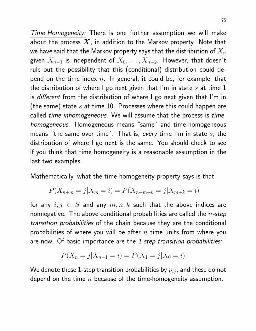
Time Homogeneity: There is one further assumption we will make

about the process X, in addition to the Markov property. Note that

we have said that the Markov property says that the distribution of Xn

given Xn−1 is independent of X0, . . . , Xn−2. However, that doesn’t

rule out the possibility that this (conditional) distribution could de-

pend on the time index n. In general, it could be, for example, that

the distribution of where I go next given that I’m in state s at time 1

is different from the distribution of where I go next given that I’m in

(the same) state s at time 10. Processes where this could happen are

called time-inhomogeneous. We will assume that the process is time-

homogeneous. Homogeneous means “same” and time-homogeneous

means “the same over time”. That is, every time I’m in state s, the

distribution of where I go next is the same. You should check to see

if you think that time homogeneity is a reasonable assumption in the

last two examples.

Mathematically, what the time homogeneity property says is that

P (Xn+m = j|Xm = i) = P (Xn+m+k = j|Xm+k = i)

for any i, j ∈ S and any m,n, k such that the above indices are

nonnegative. The above conditional probabilities are called the n-step

transition probabilities of the chain because they are the conditional

probabilities of where you will be after n time units from where you

are now. Of basic importance are the 1-step transition probabilities:

P (Xn = j|Xn−1 = i) = P (X1 = j|X0 = i).

We denote these 1-step transition probabilities by pij, and these do not

depend on the time n because of the time-homogeneity assumption.


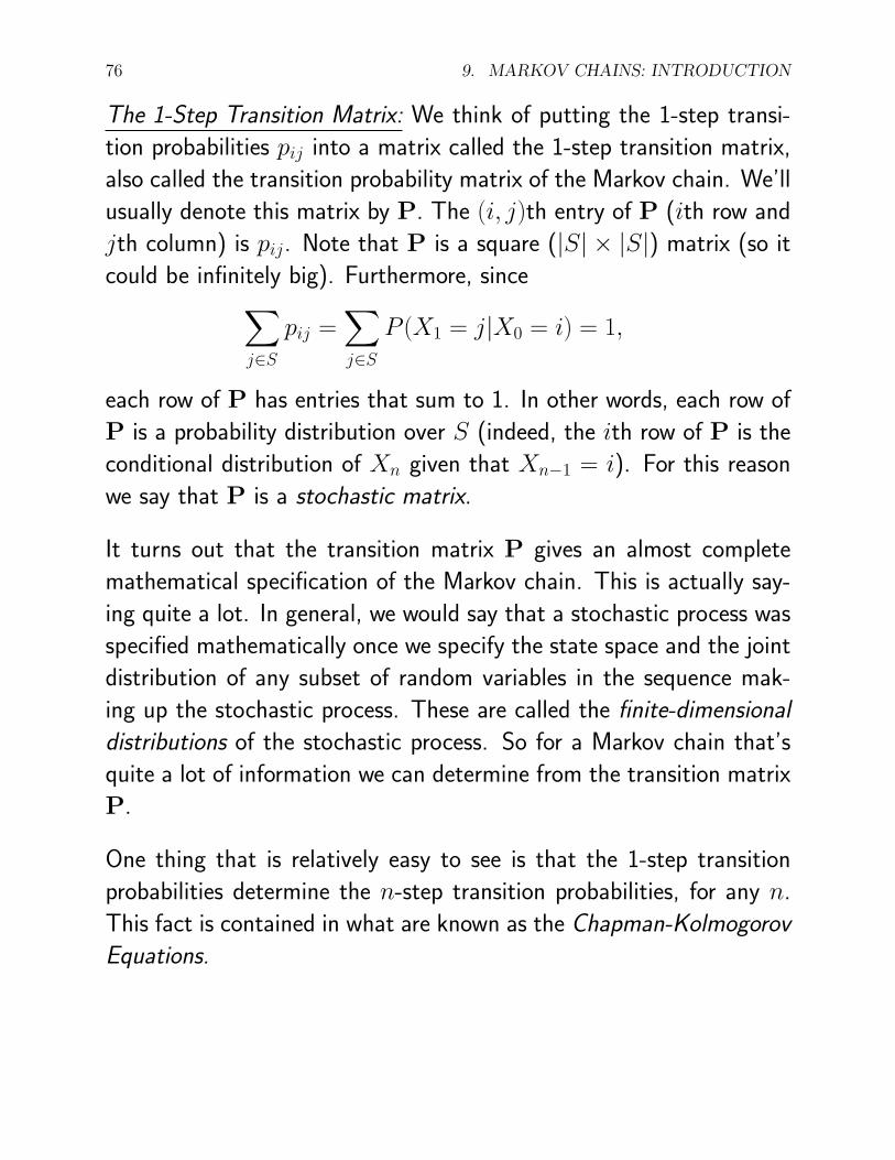
The 1-Step Transition Matrix: We think of putting the 1-step transi-

tion probabilities pij into a matrix called the 1-step transition matrix,

also called the transition probability matrix of the Markov chain. We’ll

usually denote this matrix by P. The (i, j)th entry of P (ith row and

jth column) is pij. Note that P is a square (|S| × |S|) matrix (so it

could be infinitely big). Furthermore, since∑j∈S

pij =∑j∈S

P (X1 = j|X0 = i) = 1,

each row of P has entries that sum to 1. In other words, each row of

P is a probability distribution over S (indeed, the ith row of P is the

conditional distribution of Xn given that Xn−1 = i). For this reason

we say that P is a stochastic matrix.

It turns out that the transition matrix P gives an almost complete

mathematical specification of the Markov chain. This is actually say-

ing quite a lot. In general, we would say that a stochastic process was

specified mathematically once we specify the state space and the joint

distribution of any subset of random variables in the sequence mak-

ing up the stochastic process. These are called the finite-dimensional

distributions of the stochastic process. So for a Markov chain that’s

quite a lot of information we can determine from the transition matrix

P.

One thing that is relatively easy to see is that the 1-step transition

probabilities determine the n-step transition probabilities, for any n.

This fact is contained in what are known as the Chapman-Kolmogorov

Equations.

77

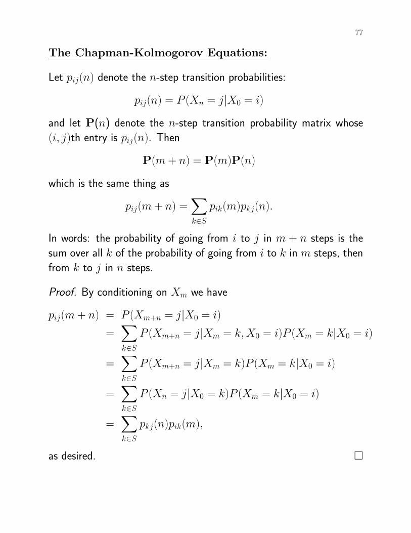
The Chapman-Kolmogorov Equations:

Let pij(n) denote the n-step transition probabilities:

pij(n) = P (Xn = j|X0 = i)

and let P(n) denote the n-step transition probability matrix whose

(i, j)th entry is pij(n). Then

P(m + n) = P(m)P(n)

which is the same thing as

pij(m + n) =∑k∈S

pik(m)pkj(n).

In words: the probability of going from i to j in m + n steps is the

sum over all k of the probability of going from i to k in m steps, then

from k to j in n steps.

Proof. By conditioning on Xm we have

pij(m + n) = P (Xm+n = j|X0 = i)

=∑k∈S

P (Xm+n = j|Xm = k,X0 = i)P (Xm = k|X0 = i)

=∑k∈S

P (Xm+n = j|Xm = k)P (Xm = k|X0 = i)

=∑k∈S

P (Xn = j|X0 = k)P (Xm = k|X0 = i)

=∑k∈S

pkj(n)pik(m),

as desired. �


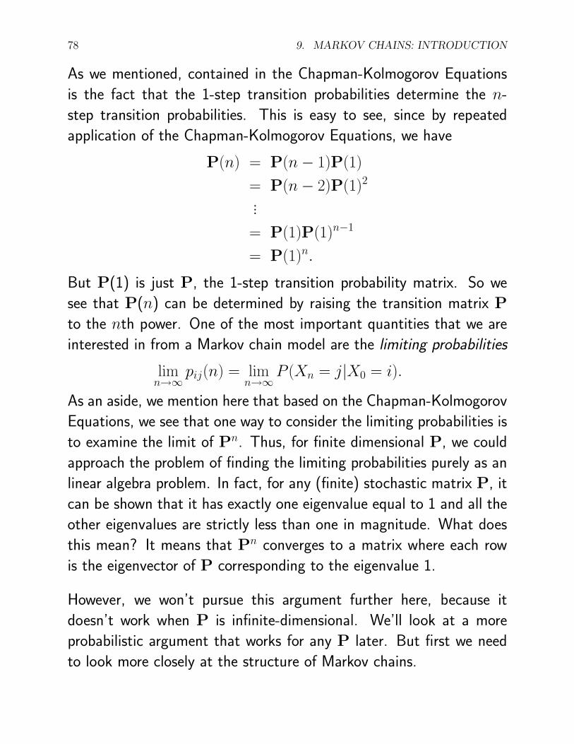
As we mentioned, contained in the Chapman-Kolmogorov Equations

is the fact that the 1-step transition probabilities determine the n-

step transition probabilities. This is easy to see, since by repeated

application of the Chapman-Kolmogorov Equations, we have

P(n) = P(n− 1)P(1)

= P(n− 2)P(1)2

...

= P(1)P(1)n−1

= P(1)n.

But P(1) is just P, the 1-step transition probability matrix. So we

see that P(n) can be determined by raising the transition matrix P

to the nth power. One of the most important quantities that we are

interested in from a Markov chain model are the limiting probabilities

limn→∞

pij(n) = limn→∞

P (Xn = j|X0 = i).

As an aside, we mention here that based on the Chapman-Kolmogorov

Equations, we see that one way to consider the limiting probabilities is

to examine the limit of Pn. Thus, for finite dimensional P, we could

approach the problem of finding the limiting probabilities purely as an

linear algebra problem. In fact, for any (finite) stochastic matrix P, it

can be shown that it has exactly one eigenvalue equal to 1 and all the

other eigenvalues are strictly less than one in magnitude. What does

this mean? It means that Pn converges to a matrix where each row

is the eigenvector of P corresponding to the eigenvalue 1.

However, we won’t pursue this argument further here, because it

doesn’t work when P is infinite-dimensional. We’ll look at a more

probabilistic argument that works for any P later. But first we need

to look more closely at the structure of Markov chains.

10

Classification of States

Let us consider a fairly general version of a Markov chain called the

random walk.

Example: Random Walk. Consider a Markov chain X with transi-

tion probabilities

pi,i+1 = pi,

pi,i = ri,

pi,i−1 = qi and

pij = 0 for all j 6= i− 1, i, i + 1,

for any integer i, where pi + ri + qi = 1. A Markov chain like this,

which can only stay where it is or move either one step up or one

step down from its current state, is called a random walk. Random

walks have applications in several areas, including modeling of stock

prices and modeling of occupancy in service systems. The random

walk is also a great process to study because it is relatively simple to

think about yet it can display all sorts of interesting behaviour that is

illustrative of the kinds of things that can happen in Markov Chains

in general.

79

80 10. CLASSIFICATION OF STATES

To illustrate some of this behaviour, we’ll look now at two special cases

of the random walk. The first is the following

Example: Random Walk with Absorbing Barriers. Let N be some

fixed positive integer. In the random walk, let

p00 = pNN = 1,

pi,i+1 = p for i = 1, . . . , N − 1,

pi,i−1 = q = 1− p for i = 1, . . . , N − 1, and

pij = 0 otherwise.

We can take the state space to be S = {0, 1, . . . , N}. The states 0

and N are called absorbing barriers, because if the process ever enters

in either of these states, the process will stay there forever after. �

This example illustrates the four possible relationships that can exist

between any pair of states i and j in any Markov chain.

1. State j is accessible from state i but state i is not accessible from

state j. This means that, starting in state i, there is a positive

probability that we will eventually go to state j, but starting in

state j the probability that we will ever go to state i is 0. In the

random walk with absorbing barriers, state N is accessible from

state 1, but state 1 is not accessible from state N .

2. State j is not accessible from state i but i is accessible from j.

3. Neither states i nor j are accessible from the other. In the random

walk with absorbing barriers, states 0 and N are like this.

4. States i and j are accessible from each other. In the random walk

with absorbing barriers, i and j are accessible from each other

for i, j = 1, . . . , N − 1. In this case we say that states i and j

communicate.

81

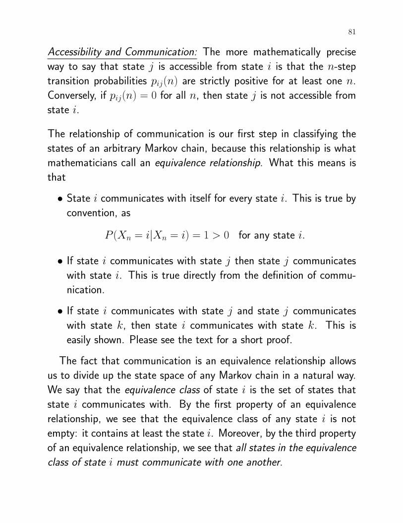
Accessibility and Communication: The more mathematically precise

way to say that state j is accessible from state i is that the n-step

transition probabilities pij(n) are strictly positive for at least one n.

Conversely, if pij(n) = 0 for all n, then state j is not accessible from

state i.

The relationship of communication is our first step in classifying the

states of an arbitrary Markov chain, because this relationship is what

mathematicians call an equivalence relationship. What this means is

that

• State i communicates with itself for every state i. This is true by

convention, as

P (Xn = i|Xn = i) = 1 > 0 for any state i.

• If state i communicates with state j then state j communicates

with state i. This is true directly from the definition of commu-

nication.

• If state i communicates with state j and state j communicates

with state k, then state i communicates with state k. This is

easily shown. Please see the text for a short proof.

The fact that communication is an equivalence relationship allows

us to divide up the state space of any Markov chain in a natural way.

We say that the equivalence class of state i is the set of states that

state i communicates with. By the first property of an equivalence

relationship, we see that the equivalence class of any state i is not

empty: it contains at least the state i. Moreover, by the third property

of an equivalence relationship, we see that all states in the equivalence

class of state i must communicate with one another.


More than that, if j is any state in the equivalence class of state i,

then states i and j have the same equivalence class. You cannot, for

example, have a state k that is in the equivalence class of j but not

in the equivalence class of i because that means k communicates with

j, and j communicates with i, but k does not communicate with i,

and this contradicts the third property of an equivalence relationship.

So that means we can talk about the equivalence class of states that

communicate with one another, as opposed to the equivalence class of

any particular state i. Now the state space of any Markov chain could

have just one equivalence class (if all states communicate with one

another) or it could have more than one equivalence class (you may

check that in the random walk with absorbing barriers example there

are three equivalence classes). But two different equivalence classes

must be disjoint because if, say, state i belonged to both equivalence

class 1 and to equivalence class 2, then again by the third property of

an equivalence relationship, every state in class 1 must communicate

with every state in class 2 (through communication with state i), and

so every state in class 2 belongs to class 1 (by definition), and vice

versa. In other words, class 1 and class 2 cannot be different unless

they are disjoint.

Thus we see that the equivalence relationship of communication di-

vides up the state space of a Markov chain into disjoint sets of equiva-

lence classes. You may wish to go over Examples 4.11 and 4.12 in the

text at this point. In the case when all the states of a Markov chain

communicate with one another, we say that the state space is irre-

ducible. We also say in this case that the Markov chain is irreducible.

More generally, we say that the equivalence relation of communication

partitions the state space of a Markov chain into disjoint, irreducible,

equivalence classes.

83

Classification of States

In addition to classifying the relationships between pairs of states,

we also can classify each individual states into one of three mutually

disjoint categories. Let us first look at another special case of the

random walk before defining these categories.

Example: Simple Random Walk. In the random walk model, if we

let

pi = p,

ri = 0, and

qi = q = 1− p

for all i, then we say that the random walk is a simple random walk.

In this case the state space is the set of all integers,

S = {. . . ,−1, 0, 1, . . .}.

That is, every time we make a jump we move up with probability p

and move down with probability 1 − p, regardless of where we are in

the state space when we jump. Suppose the process starts off in state

0. If p > 1/2, your intuition might tell you that the process will, with

probability 1, eventually venture off to +∞, never to return to the

0 state. In this case we would say that state 0 is transient, because

there is a positive probability that if we start in state 0 then we will

never return to it.

Suppose now that p = 1/2. Now would you say that state 0 is

transient? If it’s not, that is, if we start out in state 0 and it will

eventually return to state 0 with probability 1, then we say that state

0 is recurrent.


Transient and Recurrent States: In any Markov chain, define

fi = P (Eventually return to state i|X0 = i)

= P (Xn = i for some n ≥ 1|X0 = i).

If fi = 1, then we say that state i is recurrent. Otherwise, if fi < 1,

then we say that state i is transient. Note that every state in a Markov

chain must be either transient or recurrent.

There is a pretty important applied reason why we care whether a state

is transient or recurrent. Whether a state is transient or recurrent de-

termines the kinds of questions we ask about the process. I mentioned

once that the limiting probabilities limn→∞ pij(n) are very important

because these will tell us about the “long-run” or “steady-state” be-

haviour of the process, and so give us a way to predict how the system

our process is modeling will tend to behave on average. However, if

state j is transient then this limiting probability is the wrong thing to

ask about because, as we’ll see, this limit will be 0.

For example, in the random walk with absorbing barriers, it is clear

that every state is transient except for states 0 and N (why?). What

we should be asking about is not whether we’ll be in state i, say,

where 1 ≤ i ≤ N − 1, at some time point far into the future, but

other things, like, given that we start in state i, where 1 ≤ i ≤ N−1,

a) will we eventually end up in state 0 or in state N? or b) what’s the

expected time before we end up in state 0 or state N?

As another example, in the symmetric random walk with p < 1/2,

suppose we start in state B, where B is some large integer. If B is

a transient state, then the question to ask is not about the likelihood

of being in state B in the long run, but, for example, how long before

we can expect to be in state 0.

85

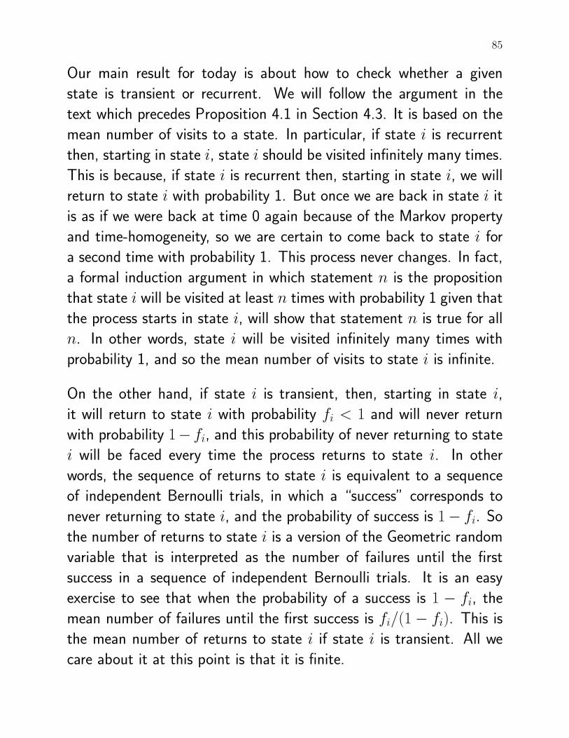
Our main result for today is about how to check whether a given

state is transient or recurrent. We will follow the argument in the

text which precedes Proposition 4.1 in Section 4.3. It is based on the

mean number of visits to a state. In particular, if state i is recurrent

then, starting in state i, state i should be visited infinitely many times.

This is because, if state i is recurrent then, starting in state i, we will

return to state i with probability 1. But once we are back in state i it

is as if we were back at time 0 again because of the Markov property

and time-homogeneity, so we are certain to come back to state i for

a second time with probability 1. This process never changes. In fact,

a formal induction argument in which statement n is the proposition

that state i will be visited at least n times with probability 1 given that

the process starts in state i, will show that statement n is true for all

n. In other words, state i will be visited infinitely many times with

probability 1, and so the mean number of visits to state i is infinite.

On the other hand, if state i is transient, then, starting in state i,

it will return to state i with probability fi < 1 and will never return

with probability 1− fi, and this probability of never returning to state

i will be faced every time the process returns to state i. In other

words, the sequence of returns to state i is equivalent to a sequence

of independent Bernoulli trials, in which a “success” corresponds to

never returning to state i, and the probability of success is 1− fi. So

the number of returns to state i is a version of the Geometric random

variable that is interpreted as the number of failures until the first

success in a sequence of independent Bernoulli trials. It is an easy

exercise to see that when the probability of a success is 1 − fi, the

mean number of failures until the first success is fi/(1− fi). This is

the mean number of returns to state i if state i is transient. All we

care about it at this point is that it is finite.


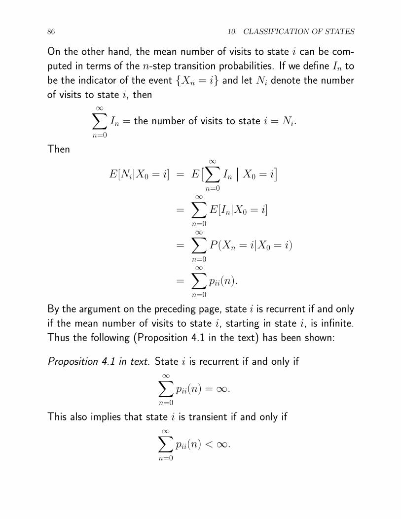
On the other hand, the mean number of visits to state i can be com-

puted in terms of the n-step transition probabilities. If we define In to

be the indicator of the event {Xn = i} and let Ni denote the number

of visits to state i, then∞∑n=0

In = the number of visits to state i = Ni.

Then

E[Ni|X0 = i] = E[ ∞∑n=0

In∣∣ X0 = i

]=

∞∑n=0

E[In|X0 = i]

=

∞∑n=0

P (Xn = i|X0 = i)

=

∞∑n=0

pii(n).

By the argument on the preceding page, state i is recurrent if and only

if the mean number of visits to state i, starting in state i, is infinite.

Thus the following (Proposition 4.1 in the text) has been shown:

Proposition 4.1 in text. State i is recurrent if and only if∞∑n=0

pii(n) = ∞.

This also implies that state i is transient if and only if∞∑n=0

pii(n) <∞.

87

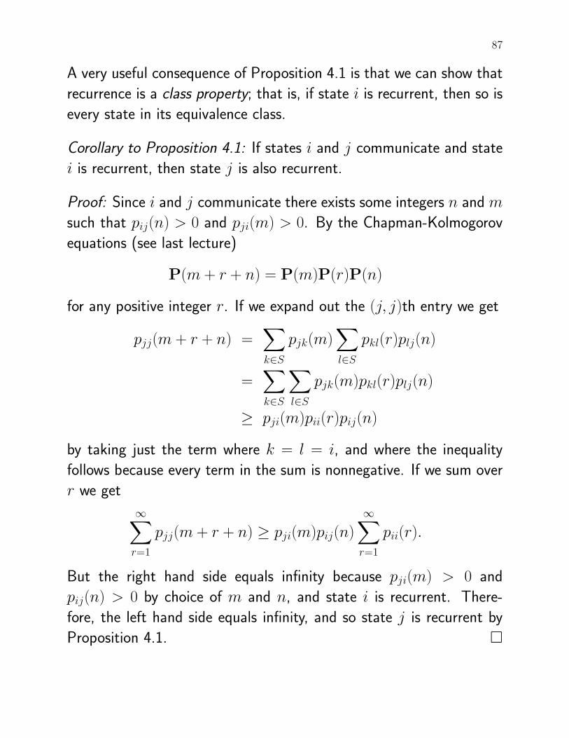
A very useful consequence of Proposition 4.1 is that we can show that

recurrence is a class property; that is, if state i is recurrent, then so is

every state in its equivalence class.

Corollary to Proposition 4.1: If states i and j communicate and state

i is recurrent, then state j is also recurrent.

Proof: Since i and j communicate there exists some integers n and m

such that pij(n) > 0 and pji(m) > 0. By the Chapman-Kolmogorov

equations (see last lecture)

P(m + r + n) = P(m)P(r)P(n)

for any positive integer r. If we expand out the (j, j)th entry we get

pjj(m + r + n) =∑k∈S

pjk(m)∑l∈S

pkl(r)plj(n)

=∑k∈S

∑l∈S

pjk(m)pkl(r)plj(n)

≥ pji(m)pii(r)pij(n)

by taking just the term where k = l = i, and where the inequality

follows because every term in the sum is nonnegative. If we sum over

r we get

∞∑r=1

pjj(m + r + n) ≥ pji(m)pij(n)

∞∑r=1

pii(r).

But the right hand side equals infinity because pji(m) > 0 and

pij(n) > 0 by choice of m and n, and state i is recurrent. There-

fore, the left hand side equals infinity, and so state j is recurrent by

Proposition 4.1. �


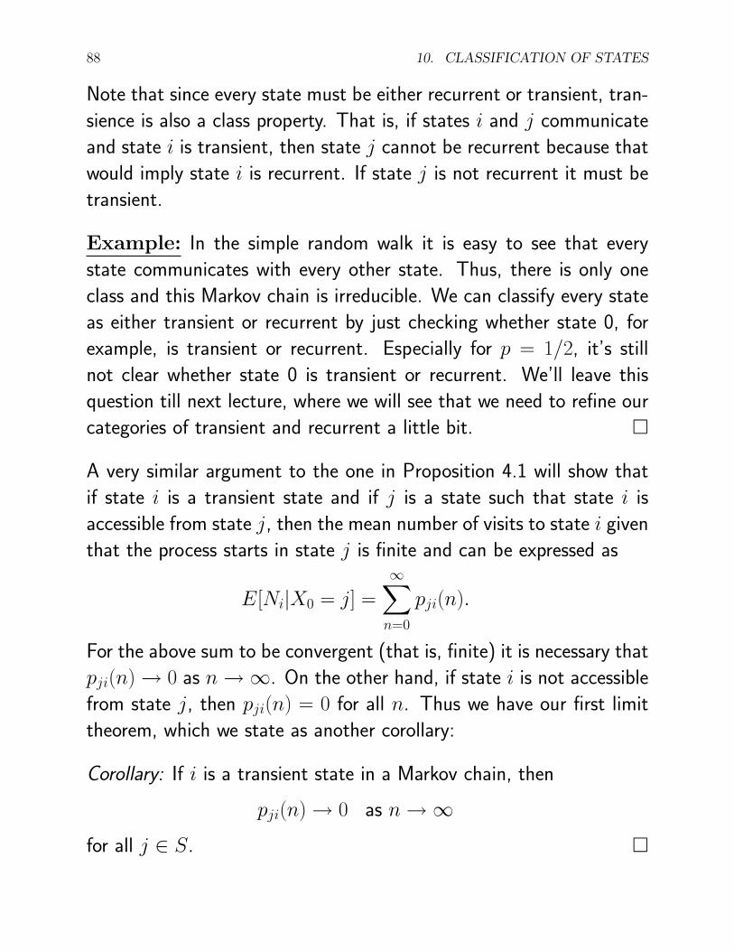
Note that since every state must be either recurrent or transient, tran-

sience is also a class property. That is, if states i and j communicate

and state i is transient, then state j cannot be recurrent because that

would imply state i is recurrent. If state j is not recurrent it must be

transient.

Example: In the simple random walk it is easy to see that every

state communicates with every other state. Thus, there is only one

class and this Markov chain is irreducible. We can classify every state

as either transient or recurrent by just checking whether state 0, for

example, is transient or recurrent. Especially for p = 1/2, it’s still

not clear whether state 0 is transient or recurrent. We’ll leave this

question till next lecture, where we will see that we need to refine our

categories of transient and recurrent a little bit. �

A very similar argument to the one in Proposition 4.1 will show that

if state i is a transient state and if j is a state such that state i is

accessible from state j, then the mean number of visits to state i given

that the process starts in state j is finite and can be expressed as

E[Ni|X0 = j] =

∞∑n=0

pji(n).

For the above sum to be convergent (that is, finite) it is necessary that

pji(n) → 0 as n→∞. On the other hand, if state i is not accessible

from state j, then pji(n) = 0 for all n. Thus we have our first limit

theorem, which we state as another corollary:

Corollary: If i is a transient state in a Markov chain, then

pji(n) → 0 as n→∞

for all j ∈ S. �

89

Since we’ve just had a number of new definitions and results, it’s

prudent at this time to recap what we have done. To summarize,

we categorized the relationship between any pair of states by defining

the (asymmetric) notion of accessibility and the (symmetric) notion

of communication. We saw that communication is an equivalence

relationship and so divides up the state space of any Markov chain

into equivalence classes. Next, we categorized the individual states

by defining the concepts of transient and recurrent. These are funda-

mental definitions in the language of Markov chain theory, and should

be memorized. A recurrent state is one that the chain will return

to with probability 1 and a transient state is one that the chain may

never return to with positive probability. Next, we proved the use-

ful Proposition 4.1 which says that state i is recurrent if and only if∑∞n=0 pii(n) is equal to infinity. Otherwise, if the sum is finite, then

state i is transient. Finally, we looked at two consequences of this

result. The first is that recurrence and transience are class properties,

and the second is that limn→∞ pji(n) = 0 if i is any transient state.

We also considered two special cases of the random walk, the random

walk with absorbing barriers and the simple random walk. The random

walk with absorbing barriers has three equivalence classes {0}, {N}and {1, . . . , N−1}. States 0 and N are recurrent states, while states

1, . . . , N − 1 are transient.

The simple random walk has just one equivalence class, so all states

are either all transient or all recurrent. However, we have not yet

determined which. Intuitively, if p < 1/2 or p > 1/2, one would guess

that all states are transient. If p = 1/2, it’s not as intuitive. What do

you think? In the next lecture we will consider this problem, and also

introduce the use of generating functions.


11

Generating Functions and the Random Walk

Today we will detour a bit from the text to look more closely at the

simple random walk discussed in the last lecture. In the process I

wish to introduce the notion and use of Generating Functions, which

are similar to Moment Generating Functions, which you may have

encountered in a previous course.

For a sequence of numbers a0, a1, a2, . . ., we define the generating

function of this sequence to be

G(s) =

∞∑n=0

snan.

This brings the sequence into another domain (where s is the argu-

ment) that is analogous to the spectral frequency domain that may

be familiar to engineers. If the sequence {an} is the probability mass

function of a random variable X on the nonnegative integers (i.e.

P (X = n) = an), then we call the generating function the probability

generating function of X, and we can write it as

G(s) = E[sX ].

91

92 11. GENERATING FUNCTIONS AND THE RANDOM WALK

Generating functions have many useful properties. Here we will briefly

go over two properties that will be used when we look at the random

walk. The first key property is how the generating function decom-

poses when applied to a convolution. If {a0, a1, . . .} and {b0, b1, . . .}are two sequences then we define their convolution by the sequence

{c0, c1, . . .}, where

cn = a0bn + a1bn−1 + . . . + anb0 =

n∑i=0

aibn−i.

The generating function of the convolution is

Gc(s) =

∞∑n=0

cnsn =

∞∑n=0

n∑i=0

aibn−isn

=

∞∑i=0

∞∑n=i

aibn−isn =

∞∑i=0

aisi∞∑n=i

bn−isn−i

= Ga(s)Gb(s),

where Ga(s) is the generating function of {an} and Gb(s) is the gen-

erating function of {bn}.

In the case when {an} and {bn} are probability distributions andX and

Y are two independent random variables on the nonnegative integers

with P (X = n) = an and P (Y = n) = bn, we see that the convolu-

tion {cn} is just the distribution of X+Y (i.e. P (X+Y = n = cn)).

In this case the decomposition above can be written as

GX+Y (s) = E[sX+Y ] = E[sXsY ] = E[sX ]E[sY ] = GX(s)GY (s),

where the factoring of the expectation follows from the independence

of X and Y . In words, the generating function of the sum of inde-

pendent random variables is the product of the individual generating

functions of the random variables.

93

The second important property that we need for now is that if GX(s)

is the generating function of a random variable X, then

G′X(1) = E[X ]

This is straightforward to see because

G′(s) =d

ds(a0 + a1s + a2s

2 + . . .)

= a1 + 2a2s + 3a3s2 + . . .

so that

G′(1) = a1 + 2a2 + 3a3 + . . . = E[X ],

assuming an = P (X = n).

In addition, one can also easily verify that if G(s) is the generating

function of an arbitrary sequence {an}, then the nth derivative of

G(s) evaluated at s = 0 is equal to n!an. That is,

G(n)(0) = n!an

and so

an =1

n!G(n)(0).

In other words, the generating function of a sequence determines the

sequence. As a special case, the probability generating function of

a random variable X determines the distribution of X. This can

sometimes be used in conjunction with the property on the previous

page to determine the distribution of a sum of independent random

variables. For example, we can use this method to show that the

sum of two independent Poisson random variables again has a Poisson

distribution. Now let’s consider the simple random walk.


Firstly, we discuss an important property of the simple random walk

process that is not shared by most Markov chains. In addition to be-

ing time homogeneous, the simple random walk has a property called

spatial homogeneity. In words, this means that if I take a portion of

a sample path (imagine a graph of the sample path with the state on

the vertical axis and time on the horizontal axis) and then displace it

vertically by any integer amount, that displaced sample path, condi-

tioned on my starting value, has the same probability as the original

sample path, conditioned on its starting value. Another way to say

this is analogous to one way that time homogeneity was explained.

That is, a Markov chain is time homogeneous because, for any state

i, every time we go into state i, the probabilities of where we go next

depend only on the state i and not on the time that we went into

state i. For a time homogeneous process that is also spatially homo-

geneous, not only do the probabilities of where we go next not depend

on the time we entered state i, but also do not depend on the state.

For the simple random walk, no matter where we are and no matter

what the time is, we always move up with probability p and down with

probability q = 1 − p. Mathematically, we say that a (discrete-time)

process is spatially homogeneous if for any times n,m ≥ 0 and any

displacement k,

P (Xn+m = b|Xn = a) = P (Xn+m = b + k|Xn = a + k).

For example, in the simple random walk the probability that we are in

state 5 at time 10 given that we are in state 0 at time 0 is the same

as the probability that we are in state 10 at time 10 given that we are

in state 5 at time 0. Together with time homogeneity, we can assert,

as another example, that the probability that we ever reach state 1

given we start in state 0 at time 0 is the same as the probability that

we ever reach state 2 given that we start in state 1 at time 1.

95

Our goal is to determine whether state 0 in a simple random walk

is transient or recurrent. Since all states communicate in a simple

random walk, determining whether state 0 is transient or recurrent

tells us whether all states are transient or recurrent. Let us suppose

that the random walk starts in state 0 at time 0. Define

Tr = time that the walk first reaches state r, for r ≥ 1

T0 = time that the walk first returns to state 0.

Also define

fr(n) = P (Tr = n|X0 = 0)

for r ≥ 0 and n ≥ 0 (noting that fr(0) = 0 for all r), and let

Gr(s) =

∞∑n=0

snfr(n)

be the generating function of the sequence {fr(n)}, for r ≥ 0. Note

that G0(1) =∑∞

n=0 f0(n) is the probability that the walk ever returns

to state 0, so this will tell us directly whether state 0 is transient or

recurrent. State 0 is transient if G0(1) < 1 and state 0 is recurrent if

G0(1) = 1. We will proceed now by first considering Gr(s), for r > 1,

then considering G1(s). We will consider G0(s) later.

To approach the evaluation of Gr(s), for r > 1, we consider the

probability fr(n) = P (Tr = n|X0 = 0) and condition on T1, the time

the walk first reaches state 1, to obtain via the Markov property that

fr(n) =

∞∑k=0

P (Tr = n|T1 = k)f1(k)

=

n∑k=0

P (Tr = n|T1 = k)f1(k),


where we can truncate the sum at n because P (Tr = n|T1 = k) = 0

for k > n (this should be clear from the definitions of Tr and T1).

Now we may apply the time and spatial homogeneity of the random

walk to consider the conditional probability P (Tr = n|T1 = k). By

temporal and spatial homogeneity, this is the same as the probability

that the first time we reach state r− 1 is at time n− k given that we

start in state 0 at time 0. That is,

P (Tr = n|T1 = k) = fr−1(n− k),

and so

fr(n) =

n∑k=0

fr−1(n− k)f1(k).

So we see that the sequence {fr(n)} is the convolution of the two

sequences {fr−1(n)} and {f1(n)}. Therefore, by the first property of

generating functions that we considered, we have

Gr(s) = Gr−1(s)G1(s).

But by applying this decomposition to Gr−1(s), and so on, we arrive

at the conclusion that

Gr(s) = G1(s)r,

for r > 1. Now we will use this result to approach G1(s). This time

we condition on X1, the first step of the random walk, to write, for

n > 1,

f1(n) = P (T1 = n|X1 = 1)p + P (T1 = n|X1 = −1)q.

Now if n > 1, then P (T1 = n|X1 = 1) = 0 because if X1 = 1 then

that implies T1 = 1 also, so that T1 = n is impossible. Also, again by

97

the time and spatial homogeneity of the random walk, we may assert

that P (T1 = n|X1 = −1) is the same as the probability that the first

time the walk reaches state 2 is at time n − 1 given that the walk

starts in state 0 at time 0. That is

P (T1 = n|X1 = −1) = f2(n− 1).

Therefore,

f1(n) = qf2(n− 1),

for n > 1. For n = 1, f1(1) is just the probability that the first

thing the random walk does is move up to state 1, so f1(1) = p. We

now have enough to write out an equation for the generating function

G1(s). Keeping in mind that f1(0) = 0, we have

G1(s) =

∞∑n=0

snf1(n)

= sf1(1) +

∞∑n=2

snf1(n)

= ps +

∞∑n=2

snqf2(n− 1)

= ps + qs

∞∑n=2

sn−1f2(n− 1)

= ps + qs

∞∑n=1

snf2(n)

= ps + qsG2(s),

since f2(0) = 0 as well.


But by our previous result we know that G2(s) = G1(s)2, so that

G1(s) = ps + qsG1(s)2,

and so we have a quadratic equation for G1(s). We may write it in

the more usual form

qsG1(s)2 −G1(s) + ps = 0.

Using the quadratic formula, the two roots of this equation are

G1(s) =1±

√1− 4pqs2

2qs.

Only one of these two roots is the correct answer. A boundary con-

dition for G1(s) is that G1(0) = f1(0) = 0. You can check (using

L’Hospital’s rule) that only the solution

G1(s) =1−

√1− 4pqs2

2qs

satisfies this boundary condition.

Let us pause for a moment to consider what we have done. We

have seen a fairly typical way in which generating functions are used

with discrete time processes, especially Markov chains. A generating

function can be defined for any sequence indexed by the nonnegative

integers. This sequence is often a set of probabilities defined on the

nonnegative integers, and obtaining the generating function of this

sequence can tell us useful information about this set of probabilities.

In fact, theoretically at least, the generating function tells us everything

about this set of probabilities, since the generating function determines

these probabilities. In our current work with the random walk, we have

defined probabilities fr(n) over the times n = 0, 1, 2, . . . at which

99

an event of interest first occurs. We may also work with generating

functions when the state space of our Markov chain is the set of

nonnegative integers and we define probabilities over the set of states.

Many practical systems of interest are modeled with a state space

that is the set of nonnegative integers, including service systems in

which the state is the number of customers/jobs/tasks in the system.

We will consider the use of generating functions again when we look

at queueing systems in Chapter 8 of the text. Note also that when

the sequence is a sequence of probabilities, a typical way that we

try to determine the generating function of the sequence is to use

a conditioning argument to express the probabilities in the sequence

in terms of related probabilites. As we have seen before, when we

do this right we set up a system of equations for the probabilites,

and as we have just seen now, this can be turned into an equation

for the generating function of the sequence. One of the advantages

of using generating functions is when we are able to compress many

(usually infinitely many) equations for the probabilities into just a single

equation for the generating function, as we did for G1(s).

So G1(s) can tell us something about the probabilities f1(n), for n ≥1. In particular

G1(1) =

∞∑n=1

P (T1 = n|X0 = 0)

= P (the walk ever reaches 1|X0 = 0)

Setting s = 1, we see that

G1(1) =1−

√1− 4pq

2q.


We can simplify this by replacing p with 1 − q in 1 − 4pq to get

1 − 4pq = 1 − 4(1 − q)q = 1 − 4q + 4q2 = (1 − 2q)2. Since√(1− 2q)2 = |1− 2q|, we have that

G1(1) =1− |1− 2q|

2q.

If q ≤ 1/2 then |1 − 2q| = 1 − 2q and G1(1) = 2q/2q = 1. On

the other hand, if q > 1/2 then |1 − 2q| = 2q − 1 and G1(1) =

(2 − 2q)/2q = 2p/2q = p/q, which is less than 1 if q > 1/2. So we

see that

G1(1) =

{1 if q ≤ 1/2

p/q < 1 if q > 1/2..

In other words, the probability that the random walk ever reaches 1 is

1 if p ≥ 1/2 and is less than 1 if p < 1/2.

Next we will finish off our look at generating functions and the random

walk by evaluating G0(s), which will tell us whether state 0 is transient

or recurrent.

12

More on Classification

Today’s lecture starts off with finishing up our analysis of the simple

random walk using generating functions that was started last lecture.

We wish to consider G0(s), the generating function of the sequence

f0(n), for n ≥ 0, where

f0(n) = P (T0 = n|X0 = 0)

= P (walk first returns to 0 at time n|X0 = 0).

We condition on X1, the first step of the random walk, to obtain via

the Markov property that

f0(n) = P (T0 = n|X1 = 1)p + P (T0 = n|X0 = −1)q.

We follow similar arguments as those in the last lecture to evaluate

the conditional probabilities. For P (T0 = n|X0 = −1), we may say

that by the time and spatial homogeneity of the random walk, this is

the same as the probability that we first reach state 1 at time n − 1

given that we start in state 0 at time 0. That is,

P (T0 = n|X0 = −1) = P (T1 = n− 1|X0 = 0) = f1(n− 1).

101

102 12. MORE ON CLASSIFICATION

By a similar reasoning, if we define T−1 to be the first time the walk

reaches state -1 and define f−1(n) = P (T−1 = n|X0 = 0), then

P (T0 = n|X1 = 1) = P (T−1 = n− 1|X0 = 0) = f−1(n− 1),

so we have so far that

f0(n) = f−1(n− 1)p + f1(n− 1)q.

Now if we had p = q = 1/2, so that on each step the walk was

equally likely to move up or down, reasoning by symmetry tells us that

P (T−1 = n − 1|X0 = 0) = P (T1 = n − 1|X0 = 0). For general p,

we can also see by symmetry that, given that we start in state 0 at

time 0, the distribution of T−1 is the same as the distribution of T1

in a “reflected” random walk in which we interchange p and q. That

is, if we let f ?1 (n) denote the probability that the first time we reach

state 1 is at time n given that we start in state 0 at time 0, but in a

random walk with p and q interchanged, then what we are saying is

that

f ?1 (n) = f−1(n)

So, keeping in mind what the ? means, we have

f0(n) = f ?1 (n− 1)p + f1(n− 1)q.

Therefore (since f0(0) = 0),

G0(s) =

∞∑n=1

snf0(n) =

∞∑n=1

snf ?1 (n− 1)p +

∞∑n=1

snf1(n− 1)q

= ps∞∑n=1

sn−1f ?1 (n− 1) + qs∞∑n=1

sn−1f1(n− 1)

= psG?1(s) + qsG1(s),

where G?1(s) is the same function as G1(s) except with p and q inter-

changed.

103

Now, recalling from the last lecture that

G1(s) =1−

√1− 4pqs2

2qs,

we see that

G?1(s) =

1−√

1− 4pqs2

2ps,

and so

G0(s) = psG?1(s) + qsG1(s)

= ps1−

√1− 4pqs2

2ps+ qs

1−√

1− 4pqs2

2qs

= 1−√

1− 4pqs2

Well, that took a bit of maneuvering, but we’ve ended up with quite

a simple form for G0(s). Now using this, it is easy to look at

G0(1) =

∞∑n=1

f0(n) = P (walk ever returns to 0|X0 = 0).

Plugging in s = 1, we get

G0(1) = 1−√

1− 4pq.

As we did before, we can simplify this by writing 1− 4pq = 1− 4(1−q)q = 1− 4q + 4q2 = (1− 2q)2, so that

G0(1) = 1− |1− 2q|.

Now we can see that if q ≤ 1/2 then G0(1) = 1 − (1 − 2q) = 2q.

This equals one if q = 1/2 and is less than one if q < 1/2. On the

other hand, if q > 1/2 then G0(1) = 1 − (2q − 1) = 2 − 2q = 2p,

and this is less than one when q > 1/2.


So we see that G0(1) is less than one if q 6= 1/2 and is equal to one if

q = 1/2. In other words, state 0 is transient if q 6= 1/2 and is recurrent

if q = 1/2. Furthermore, since all states in the simple random walk

communicate with one another, there is only one equivalence class, so

that if state 0 is transient then all states are transient and if state 0 is

recurrent then all states are recurrent. This should also be intuitively

clear by the spatial homogeneity of the random walk. In any case, it

makes sense to say that the random walk is transient if q 6= 1/2 and

is recurrent if q = 1/2.

Now we remark here that we have just seen that the “random vari-

ables”, Tr, in some cases had distributions that did not sum up to one.

For example, as we have just seen∞∑n=1

P (T0 = n|X0 = 0) < 1

if q 6= 1/2. This is because, for q 6= 1/2, it is the case that P (T0 =

∞|X0 = 0) > 0. In words, T0 equals infinity with positive probability.

According to what you should have learned in a previous probability

probability course, this disqualifies T0 to be called a random variable

when q 6= 1/2. In fact, we say in this case that T0 is a defective random

variable. Defective random variables can arise sometimes in the study

of stochastic processes, especially when the random quantity, let’s call

it, denotes a time until the process first does something, like reach a

certain state or set of states, because it may be that the process will

never reach that set of states with some positive probability. In fact,

knowing that a process may never reach a state or set of states with

some positive probability is of central interest for some systems, such

as population models where we want to know if the population will

ever die out.

105

In the case where q = 1/2, of course, T0 is a proper random variable.

Here let us go back to the second property of generating functions

that we covered last lecture, which is that for a random variable X

with probability generating function GX(s), the expected value of X

is given by

E[X ] = G′X(1).

When q = 1/2, the random variable T0 has probability generating

function

G0(s) = 1−√

1− s2,

so that taking the derivative we get

G′0(s) =

s√1− s2

.

Setting s = 1 we see that G′0(1) = +∞. That is, E[T0] = +∞ when

q = 1/2. So even though state 0 is recurrent when q = 1/2, we have

here an illustration of a very special kind of recurrent state. Starting

in state 0, we will return to state 0 with probability one, and so state

0 is recurrent. But the expected time to return to state 0 is +∞. In

such a case we call the recurrent state a null recurrent state. This is

another important classification of a state which we discuss next.

Remark: The text uses a more direct approach, using Proposition 4.1,

to determine the conditions under which a simple random walk is tran-

sient or recurrent. Please read Example 4.13 to see this solution. Our

approach using generating functions was chosen in part to introduce

generating functions, which have uses much beyond analysing the sim-

ple random walk. We were also able to obtain more information about

the random walk using generating functions.


Null Recurrent and Positive Recurrent States. Recurrent states in a

Markov chain can be further categorized as null recurrent and positive

recurrent, depending on the expected time to return to the state. If

µi denotes the expected time to return to state i given that the chain

starts in state i, then we say that state i is null recurrent if it is

recurrent (i.e. P (eventually return to state i|X0 = i) = 1) but the

expected time to return is infinite:

State i is null recurrent if µi = ∞.

Otherwise, we say that state i is positive recurrent if it is recurrent

and the mean time to return is finite:

State i is positive recurrent if µi <∞.

A null recurrent state i is, like any recurrent state, returned to infinitely

many times with probability 1. Even so, the probability of being in a

null recurrent state is 0 in the limit:

limn→∞

pji(n) = 0,

for any starting state j. This interesting fact is something we’ll prove

later. A very useful fact, that we’ll also prove later, is that null recur-

rence is a class property. We’ve already seen that recurrence is a class

property. This is stronger. Not only do all states in an equivalence

class have to be recurrent if one of them is, they all have to be null

recurrent if one of them is. This also implies that they all have to be

positive recurrent if one of them is.

So we see that the equivalence relationship of communication divides

up any state space into disjoint equivalence classes, and each equiva-

lence class has “similar” members, in that they are either all transient,

all null recurrent, or all positive recurrent.

107

A finite Markov chain has at least one positive recurrent state: The

text (on p.192) argues that a Markov chain with finitely many states

must have at least one recurrent state. The argument is basically that

not all states can be transient because if this were so then eventually

we would run out of states to “never return to” if there are only finitely

many states. We can also show that a Markov chain with finitely many

states must have at least one positive recurrent state, which is slightly

stronger. In particular, this implies that any finite Markov chain

that has only one equivalence class has all states being

positive recurrent.

Since we must be somewhere at time n, we must have∑

j∈S pij(n) =

1 for any starting state i. That is, each n-step transition matrix P(n)

is a stochastic matrix (the ith row is the distribution of where the

process will be n steps later, starting in state i). This is true for every

n, so we can take the limit as n→∞ and get

limn→∞

∑j∈S

pij(n) = 1.

But if S is finite, we can take the limit inside to get

1 =∑j∈S

limn→∞

pij(n).

But if every state were transient or null recurrent we would have

limn→∞ pij = 0 for every i and j. Thus we would get the contra-

diction that 1=0. Thus, there must be at least one positive recurrent

state. Keep in mind that limits cannot in general be taken inside sum-

mations if it is an infinite sum. For example, limn→∞∑∞

j=1 1/n 6=∑∞j=1 limn→∞ 1/n. The LHS is +∞ and the RHS is 0.


Recurrent Classes are Closed. Now, in general, the state space of a

Markov chain could have 1 or more transient classes, 1 or more null

recurrent classes, and 1 or more positive recurrent classes. While state

spaces with both transient and recurrent states are of great practical

use (and we’ll look at these in Section 4.6), many practical systems

of interest are modeled by Markov chains for which all states are re-

current, and usually all positive recurrent. Even in this case, one can

imagine that there could be 2 or more disjoint classes of recurrent

states. The following Lemma says that when all states are recurrent

we might as well assume that there is only one class because if we are

in a recurrent class we will never leave it. In other words, we say that

a recurrent class is closed.

Lemma: Any recurrent class is closed. That is, if state i is recurrent,

and state j is not in the equivalence class containing state i, then

pij = 0.

Proof. Suppose we start the chain in state i. If pij were postive, then

with positive probability we could go to state j. But once in state j we

could never go back to state i because if we could then i and j would

communicate. This is impossible because j is not in the equivalence

class containing i, by assumption. But never going back to state i is

also impossible because state i is recurrent by assumption. Therefore,

it must be that pij = 0. �

Therefore, if all states are recurrent (null or positive recurrent) and

there is more than one equivalence class, we may as well assume that

the state space consists of just the equivalence class that the chain

starts in.

109

Period of a State:

There is one more property of a state that we need to define, and that

is the period of a state. In words, the period of a state i is the largest

integer that evenly divides all the possible times that we could return

to state i given that we start in state i. If we let di denote the period

of state i, then mathematically we write this as

di = Period of state i = gcd{n : pii(n) > 0},

where “gcd” stands for “greatest common divisor”. Another way to

say this is that if we start in state i, then we cannot return to state i

at any time that is not a multiple of di.

Example: For the simple random walk, if we start in state 0, then

we can only return to state 0 with a positive probability at times

2, 4, 6, . . .; that is, only at even times. The greatest divisor of this set

of times is 2, so the period of state 0 is 2. �

If a state i is positive recurrent, then we will be interested in the

limiting probability limn→∞ pii(n). But before we do so we need to

know the period of state i. This is because if di ≥ 2 then pii(n) = 0

for any n that is not a multiple of di. But then this limit will not exist

unless it is 0 because the sequence {pii(n)} has infinitely many 0’s

in it. It turns out that the subsequence {pii(din)} will converge to a

nonzero limiting value.

If the period of state i is 1, then we are fine. The sequence {pii(n)}will have a proper limiting value. We call a state that has period 1

aperiodic.


Period is a Class Property. As we might have come to expect and

certainly hope for, our last result for today is to show that all states

in an equivalence class have the same period.

Lemma: If states i and j communicate they have the same period.

Proof. Let di be the period of state i and dj be the period of state j.

Since i and j communicate, there is somem and n such that pij(m) >

0 and pji(n) > 0. Using the Chapman-Kolmogorov equations again

as we did on Monday, we have that

pii(m + r + n) ≥ pij(m)pjj(r)pji(n),

for any r ≥ 0, and the right hand side is strictly positive for any r such

that pjj(r) > 0 (because pij(m) and pji(n) are both strictly positive.

Setting r = 0, we have pjj(0) = 1 > 0, so pii(m+n) > 0. Therefore,

di divides m + n. But since pii(m + r + n) > 0 for any r such that

pjj(r) > 0 we have that di divides m+r+n for any such r. But since

di divides m+ n it must also divide r. That is, di divides and r such

that pjj(r) > 0. In other words, di is a divisor of {r : pjj(r) > 0}.Since dj is, by definition, the greatest common divisor of the above set

of r values, we must have di ≤ dj. Now repeat the same argument

but interchange i and j, to get dj ≥ di. Therefore, di = dj. �

By the above lemma, we can speak of the period of a class, and if

a Markov chain has just one class, then we can speak of the period

of the Markov chain. In particular, we will be interested for the next

little while in Markov chains that are irreducible (one class), aperiodic

(period 1) and positive recurrent. It is these Markov chains for which

the limiting probabilities both exist and are not zero. We call such

Markov chains ergodic.

Documents

Markov Chains: Introductionstat455/lecturenotes/set2.pdf · 72 9. MARKOV CHAINS: INTRODUCTION Markov Chains: A discrete-time stochastic process Xis said to be a Markov Chain if it