Markov Chains on Countable State Space

1 Markov Chains Introduction

1. Consider a discrete time Markov chain {Xi, i = 1, 2, ...} that takes values on a countable(finite or infinite) set S = {x1, x2, ...}, where xi is the i-th state, the state of thestochastic process at time i.

Examples of countable S are:

• Zd, d dimensional integers lattice

• set of all partitions of {1, 2, ..., n}• set of all configurations of magnetic spins (-1 or 1) of a n × n lattice grid (Ising

model)

• set of possible moves of a king on a chess board

• set of possible route of visitation of n cities (traveling salesman problem)

• set of all length d vectors of 0’s and 1’s

• any finite set

It can be viewed as a stochastic process Xi indexed over time i = 1, 2, .... It is calleda Markov chain if it satisfies the Markov property: the next state Xi+1 depends onlyon the current state Xi (memoryless property), i.e.

P (Xi+1 = xj|Xi = xi, · · · , X0 = x0)

= P (Xi+1 = xj|Xi = xi).

The probability Pij = P (Xi+1 = xj|Xi = xi) is called the transition matrix. Any rowof a transition matrix will sum to one, i.e.,

∑j Pij = 1 for all i. The initial distribution

for X0 determine the distribution for any n-th state.

2. Random walk. You play a coin tossing game. You win $1 if a head appears and lose $1if a tail appears. Let Xi be your total gain after i tosses. Assume the coin is unbiased,then the transition matrix is given by

P (Xi+1 = x + 1|Xi = x) =1

2,

P (Xi+1 = x− 1|Xi = x) =1

2.

We can model the coin tossing a simple random walk Xi+1 = Xi + εi, with P (εi =1) = 1

2and P (εi = −1) = 1

2. The expected pay off does not change over time, i.e.

EXi+1 = EXi.

In this case, Xi+1 =∑n

j=0 εj + X0. Then P (Xn+1 = x|X0 = 0) = P (∑n

j=0 εj = x).Please compute this probability.

1

3. Chapman-Kolmogorov equation. Let P nxy be the transition kernel from x to y in n-steps,

i.e. P nxy = P (Xi+n = y|Xi = x). Then we have

Pm+nxy =

∑z

PmxzP

nzy.

The the probability of reaching y from x in n-steps is the sum of all probabilities goingfrom x to y through an intermediate point z.

Let Pn = (P nij) be a matrix.

Then in terms of matrix, Chapman-Kolomogorov equation can be trivially written asPm+n = PmPn.

4. Example. A rat became insane and moves back and forth between position 1 and2. Let Xi be the position of the rat at the i-th move. Suppose that the transitionprobability is given by

P =

[12

12

1 0

].

On a finite state space, a state i is called recurrent if the Markov chain returns to iwith probability 1 in a finite number of steps otherwise the state is transient. Therecurrent of a state is equivalent to a guarantee of a sure return. Is the state 1 and 2recurrent? ∞∑

i=2

P (Xi = j|X0 = j, X1 6= j, · · ·Xi−1, 6= j)

=1

2+

1

22+ · · · = 1

for j = 1, 2. So the state 1 and 2 are recurrent.

5. Let us find P (Xn = 1|X0 = 2). Note that this is n step transition probability denotedby P n

12. It is computed by the Chapman-Kolmogorov equation. For this we needto compute Pn. In general there are theorems to do this. We are glad to do thiscomputationally for now and find out that

P = 0.5 0.5

1 0

P^2 = 0.75000 0.25000

0.50000 0.50000

P^5 = 0.65625 0.34375

0.68750 0.31250

P^100 = 0.66667 0.33333

0.66667 0.33333

So we can see that the transition probabilities converge: limn→∞ P nij = πj. π1 = 2

3and

π2 = 13.

2

6. Suppose we have a probability distribution π defined on a state space S = {x1, x2, ...}such that πj = P (X = xj). We have

∑j∈S πj = 1. Then π is a stationary distribution

for the Markov chain with transition probability P if π′ = π′P.

An interesting property on πj is that it is the expected number of states a Markovchain should take to return to the original state j.

In our crazy rat example, the rat will return to position 2 in average 3 steps if it wasat the position 2 initially.

7. An increased stability for a Markov chain can be achieved if we let X0 ∼ π, i.e.P (X0 = j) = πj. We have X1 ∼ π′P = π′. Similarly Xi ∼ π.

Note that π is the eigenvector corresponding to the eigenvalue 1 for thematrix P.

Actually you don’t need to have X0 ∼ π to have a stable chain. If X0 ∼ µ for anyprobability distribution, µ′Pn → π′ as n →∞.

8. In general, the Markov chain is completely specified in terms of the distribution of theinitial state X0 ∼ µ and the transition probability matrix P

9. This is the basis of MCMC. Given probability distribution π, we want to estimate somefunctions of π, e.g., Eπg(X). The idea is to construct a Markov chain Xi and let thechain run a long time (burn in stage) so that it will converge to its stationary distrib-ution π. We then sample from an dependent sample from this stationary distributionand use it to estimate the integral function.

The difference between MCMC and a simple Monte-Carlo method is that MCMCsample are dependent and and simple Monte Carlo sample are independent.

2 Markov Chains Concepts

We want to know:Under what conditions will the chain will converge?What is the stationary distribution it converges to?We will talk about finite state space first, then extend it to infinite countable space

2.1 Markov Chains on Finite S

One way to check for convergence and stationarity is given by the following theorem:

Peron-Frobenius Theorem If there exists a positive integer n such that P nij > 0,∀i, j (i.e.,

all the elements of P n are strictly positive), then the chain will converge to the stationarydistribution π.

3

Although the condition required in Peron-Frobenious theorem is easy to state, sometimesit is difficult to establish for a given transition matrix P . Therefore, we seek another way tocharacterize the convergence of a Markov chain with conditions that may be easier to check.

For finite state space, the transition matrix needs to satisfy only two properties for theMarkov chain to converge. They are: ireducibility and aperiodicity.

Irreducibility implies that it is possible to visit from any state to any state in a finitenumber of steps. In other words, the chain is able to visit the entire S from any startingpoint X0.

Aperiodicity implies that the Markov chain does not cycle around in the states with afinite period. The problem with periodicity is limiting the chain to return to certain statesat some constant time intervals.

Some definitions:

1. Two states are said to communicate if it is possible to go from one to another in a finitenumber of steps. In other words, xi and xj are said to communicate if there exists apositive integer such that P n

ij > 0.

2. A Markov chain is said to be irreducible if all states communicate with each other forthe corresponding transition matrix.

For the above example, the Markov chain resulting from the first transition matrix willbe irreducible while the chain resulting from the second matrix will be reducible intotwo clusters: one including states x1 and x2, and the other including the states x3 andx4.

3. For a state xi and a given transition matrix Pij, define the period of xi as d(xi) =GCD{n : P n

i,i > 0}, where GCD implies the greatest common divisor.

4. If two states communicate, then it can proved that their periods are the same.

Thus, in an irreducible Markov chain where all the states communicate, they all havethe same period. This is called the period of an irreducible Markov chain.

5. An irreducible Markov chain is called aperiodic if its period is one.

6. (Theorem) For a irreducible and aperiodic Markov chain on a finite state space,it can be shown that the chain will converge to a stationary distribution.

If we let the chain run for long time, then the chain can be view as a sample from its(unique) stationary probability distribution.

These two conditions also imply: that all the entries of P nij are positive for some positive

integer n. The requirement needed for the Peron-Frobenius Theorem.

4

2.2 Markov Chains on Infinite but countable S

1. In case of infinite but countable state space, the Markov chain convergence requires anadditional concept — positive recurrence — to ensure that the chain has a uniquestationary probability.

2. The state xi is recurrent iff P (the chain starting from xi returns to xi infinitely often)= 1. A state is said to be transient if it is not recurrent.

3. It can be shown that a state is recurrent iff

∞∑n=0

P nii = ∞

4. Another way to look at recurrent/transient: A state i is said to be transient if, giventhat we start in state i, there is a non-zero probability that we will never return backto i. Formally, let the random variable Ti be the next return time to state i

Ti = min{n : Xn = i|X0 = i)

Then, state i is transient if Ti is not finite with some probability, i.e., P (Ti < ∞) < 1.

If a state i is not transient, i.e., P (Ti < ∞) = 1 (it has finite hitting time withprobability 1), then it is said to be recurrent.

Although the hitting time is finite, it need not have a finite average. Let Mi be theexpected (average) return time, state i is said to be positive recurrent if Mi is finite;otherwise, state i is null recurrent.

5. If two states xi and xj communicate, and xi is (positive) recurrent, then xj is also(positive) recurrent.

6. (Theorem) For a irreducible, aperiodic, and positive recurrent Markov chainon a countably infinite state space, it can be shown that the chain will converge toa stationary distribution. This chain is said to be ergodic.

3 Markov Chains Examples

1. Let P

P =

12

12

014

12

14

0 13

23

The eigenvector corresponding to the eigenvalue 1 for the matrix P is the stationarydistribution

5

π = (2

9

4

9

3

9)

2. Consider a Markov chain with the following transition probability matrix

P =

0 1 0 0 0

0.5 0 0.5 0 00 0.5 0 0.5 00 0 0.5 0 0.50 0 0 1 0

Calculate: Pn

if n is even:

Pn =

0.25 0 0.50 0 0.250 0.50 0 0.50 0

0.25 0 0.50 0 0.250 0.50 0 0.50 0

0.25 0 0.50 0 0.25

and if n is odd:

Pn =

0 0.50 0 0.50 0

0.25 0 0.50 0 0.250 0.50 0 0.50 0

0.25 0 0.50 0 0.250 0.50 0 0.50 0

The Markov chain is irreducible because there exists a n such that P n

ij > 0 for all i, j

Periodic with period d = 2

It means that starting in state 1, for example, P n1,1 > 0 at times n = 2, 4, 6, 8, .... and

the greatest common divisor of the values that n can take is 2.

The unique stationary distribution is

π = limn−→∞

1

2(π(n) + π(n+1))

= (0.125 0.25 0.25 0.25 0.125)

we can verify that the eigenvalues of P are −1, 0, 1,−1/√

2, 1/√

2

and there are d = 2 eigenvalues with absolute value 1

6

3. Let

P =

1 0 0 0 0

0.5 0 0.5 0 00 0.5 0 0.5 00 0 0.5 0 0.50 0 0 0 1

this system has 5 different stationary distributions for large n :

Calculate Pn

limn−→∞

Pn =

1 0 0 0 0

0.75 0 0 0 0.250.50 0 0 0 0.500.25 0 0 0 0.750 0 0 0 1

The rows of Pn represent the five stationary distributions, and each of these satisfyπ′ = π′P

4. Let

P =

12

12

0 0 016

16

0 0 00 0 3

414

00 0 3

241624

524

0 0 0 16

56

limn−→∞

Pn =

0.25 0.75 0 0 00.25 0.75 0 0 00 0 0.182 0.364 0.4550 0 0.182 0.364 0.4550 0 0.182 0.364 0.455

The chain splits into two sub-chain, each converges to a stationary distribution andone can not move from state spaces {0, 1} to states {2, 3, 4}. The resulting stationarydistribution depends on the starting point X0.

5. Ehrenfest Model

The general model will be easily extended. For now, consider two urns that, betweenthem, contain four balls. At each step, one of the four balls is chosen at random and

7

moved from the urn that it is in into the other urn. We choose, as states, the numberof balls in the first urn.

The transition matrix is

P =

0 1 0 0 014

0 34

0 00 1

20 1

20

0 0 34

0 14

0 0 0 1 0

The stationary distribution is π = (.0625, .2500, .3750, .2500, .0625).

Meaning: we can interpret πi as the proportion of times the process is in each of thestates in the long run. For example, the proportion of times in state 0 is .0625 and theproportion of times in state 1 is .375.

Note that these numbers are the binomial distribution 1/16, 4/16, 6/16, 4/16, 1/16.We could have guessed this answer as follows: If we consider a particular ball, itsimply moves randomly back and forth between the two urns. This suggests that theequilibrium state should be just as if we randomly distributed the four balls in the twourns. If we did this, the probability that there would be exactly j balls in one urnwould be given by the binomial distribution Binomial(n, p) with n = 4 and p = .5.

Let us consider the Ehrenfest model for gas diffusion for the general case of 2n balls.Every second, one of the 2n balls is chosen at random and moved from the urn it wasin to the other urn.

What is the transition matrix?

What is the stationary distribution π?

What is the mean recurrence time for state i?

6. Stepping Stone Model

This model is often used as an illustration in the study of genetics. In this modelwe have an n × n array of squares, and each square is initially any one of k differentcolors. For each step, a square is chosen at random. This square then chooses one of itseight neighbors at random and assumes the color of that neighbor. To avoid boundaryproblems, we assume that if a square s is on the left-hand boundary, say, but not at acorner, it is adjacent to the square t on the right-hand boundary in the same row as s,and s is also adjacent to the squares just above and below t. A similar assumption ismade about squares on the upper and lower boundaries. (These adjacencies are mucheasier to understand if one imagines making the array into a cylinder by gluing the topand bottom edge together, and then making the cylinder into a doughnut by gluing thetwo circular boundaries together.) With these adjacencies, each square in the array isadjacent to exactly eight other squares.

8

A state in this Markov chain is a configuration of the k colors on each square of then× n array. Thus, the Markov chain has a total of kn2

possible states.

What is the long term behavior of this chain?

What are the two absorbing states? What is the probability that eventually the chainwill stop at one absorbing state?

What is the mean number of steps for the chain to stop eventually?

7. Random Walk Model on Integers Consider the random walk on the real line ofintegers

P (Xi+1 = x + 1|Xi = x) = p

P (Xi+1 = x− 1|Xi = x) = 1− p

with X0 = 0?

It can be shown that the chain is null recurrent when p = .5 (symmetric randomwalk), and transient when p 6= .5.

8. Symmetric Random Walk on Integers on k-dimension

For k = 1, the mean distance between start and finish points in n steps is of the orderof√

n.

Every integer point will be visited infinitely often, but the expected return time isinfinite (null recurrent).

This property has many names: the level-crossing problem, the recurrence problem, orthe gambler’s ruin problem. The interpretation of the last name is as follows: if youare a gambler with a finite amount of money playing a fair game against a bank withan infinite amount of money, you will surely lose.

For k = 2, it can be shown that a symmetric random walk in two dimension is alsonull recurrent.

For k ≥ 3, the symmetric random walk is transient! Too many rooms to ”get lost”forever!

The trajectory of a random walk is the collection of integer points the chain visited,regardless of visit orders at the point. In one dimension, the trajectory is simply allpoints between the minimum and the maximum visits. In higher dimensions the sethas interesting geometric properties. In fact, one gets a discrete fractal, that is a setwhich exhibits stochastic self-similarity on large scales, but on small scales one canobserve ”jugginess” resulting from the grid on which the walk is performed. (cf. Afamous fractal is the Mandelbrot Set)

9. Random Walk Model on Non-negative Integers Consider the random walk onthe real line of non-negative integers. With X0 = 0, let the transition matrix of thechain be

P (Xi+1 = x + 1|Xi = x) = p

9

Mandelbrot Set.png

P (Xi+1 = x− 1|Xi = x) = 1− p

∀x > 0. When x = 0,P (Xi+1 = 1|Xi = 0) = p

P (Xi+1 = 0|Xi = 0) = 1− p

It can be shown that the chain is

• positive recurrent when p < .5

• null recurrent when p = .5

• transient when p > .5

10

4 Reversible Markov chain

Consider a Markov chain with state space S that converges to a stationary distribution π.Let x ∈ S denote the current state of the system.Let y ∈ S denote the current state at the next step.

Let p(x, y) denote the probability of a transition from x to yThus p(y, x) is the probability of a transition from y to x.

A Markov chain is said to be reversible if it satisfies the detail balance condition:

π(x)p(x, y) = π(y)p(y, x)

Note:

π(x)p(x, y) = P (Xn = x)P (Xn+1 = y|Xn = x) (1)

= P (Xn = x, Xn+1 = y), ∀x, y ∈ S. (2)

So the reversibility condition can also be written as

P (Xn = x, Xn+1 = y) = P (Xn = y, Xn+1 = x), ∀x, y ∈ S.

As seen later, the reversibility condition will be important in deriving the appropriatetransition kernels function for the Metropolis algorithm or other Markov chain.

5 Historical Remarks

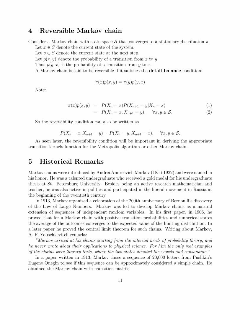
Markov chains were introduced by Andrei Andreevich Markov (1856-1922) and were named inhis honor. He was a talented undergraduate who received a gold medal for his undergraduatethesis at St. Petersburg University. Besides being an active research mathematician andteacher, he was also active in politics and participated in the liberal movement in Russia atthe beginning of the twentieth century.

In 1913, Markov organized a celebration of the 200th anniversary of Bernoulli’s discoveryof the Law of Large Numbers. Markov was led to develop Markov chains as a naturalextension of sequences of independent random variables. In his first paper, in 1906, heproved that for a Markov chain with positive transition probabilities and numerical statesthe average of the outcomes converges to the expected value of the limiting distribution. Ina later paper he proved the central limit theorem for such chains. Writing about Markov,A. P. Youschkevitch remarks:

”Markov arrived at his chains starting from the internal needs of probability theory, andhe never wrote about their applications to physical science. For him the only real examplesof the chains were literary texts, where the two states denoted the vowels and consonants.”

In a paper written in 1913, Markov chose a sequence of 20,000 letters from Pushkin’sEugene Onegin to see if this sequence can be approximately considered a simple chain. Heobtained the Markov chain with transition matrix

11

vowel consonant

vowel .128 .872

consonant .663 .337

The limiting distribution for this chain is (.432, .568), indicating that we should expectabout 43.2 percent vowels and 56.8 percent consonants in the novel, which was borne out bythe actual count.

Claude Shannon considered an interesting extension of this idea in his book The Mathe-matical Theory of Communication, in which he developed the information theoretic conceptof entropy. Shannon considers a series of Markov chain approximations to English prose.He does this first by chains in which the states are letters and then by chains in which thestates are words. For example, for the case of words he presents first a simulation where thewords are chosen independently but with appropriate frequencies.

REPRESENTING AND SPEEDILY IS AN GOOD APT OR COME CAN DIFFERENTNATURAL HERE HE THE A IN CAME THE TO OF TO EXPERT GRAY COME TOFURNISHES THE LINE MESSAGE HAD BE THESE.

He then notes the increased resemblance to ordinary English text when the words arechosen as a Markov chain, in which case he obtains

THE HEAD AND IN FRONTAL ATTACK ON AN ENGLISH WRITER THAT THECHARACTER OF THIS POINT IS THEREFORE ANOTHER METHOD FOR THE LET-TERS THAT THE TIME OF WHO EVER TOLD THE PROBLEM FOR AN UNEX-PECTED.

A simulation like the last one is carried out by opening a book and choosing the firstword, say it is the. Then the book is read until the word the appears again and the wordafter this is chosen as the second word, which turned out to be head. The book is then readuntil the word head appears again and the next word, and, is chosen, and so on.

Other early examples of the use of Markov chains occurred in Galton’s study of theproblem of survival of family names in 1889 and in the Markov chain introduced by P. andT. Ehrenfest in 1907 for diffusion. Poincare in 1912 discussed card shuffling in terms of anergodic Markov chain defined on a permutation group. Brownian motion, a continuous timeversion of random walk, was introduced in 1900-1901 by L. Bachelier in his study of thestock market, and in 1905-1907 in the works of A. Einstein and M. Smoluchowsky in theirstudy of physical processes.

12

Fractal Mandelbrot Set.jpg

13