Discrete numerical modeling of loose soil with spherical

Noname manuscript No.(will be inserted by the editor)

Discrete numerical modeling of loose soil with sphericalparticles and interparticle rolling friction

Rodaina Aboul Hosn · Luc Sibille · Nadia Benahmed · Bruno Chareyre

Published as Aboul Hosn, R., Sibille, L., Benahmed, N. and Chareyre, B. Granular Matter (2017) 19: 4.https://doi.org/10.1007/s10035-016-0687-0

Abstract Discrete numerical simulations were carried

out to reproduce experimental results obtained on loose

cohesionless soil samples subjected to triaxial tests. Pe-

riodic boundary conditions were adopted and 3D spher-

ical discrete elements were chosen. However, to over-

come excessive rolling of such an oversimplified parti-

cle’s shape, contact rolling resistance was taken into

consideration. The influence of both the elastic and the

plastic local parameters is discussed. It is shown that

the plastic macroscopic behavior of the granular assem-

bly depends only on the plastic parameters at the mi-

croscopic scale, and mainly on the plastic rolling mo-

ment reflecting the particle’s shape. Moreover, a proce-

dure to obtain an initial density, ranging from loose to

dense samples, is proposed by adding adhesion at con-

tacts during the preparation phase. Finally, a calibra-

tion procedure is proposed to reproduce experimental

results and the limitations of the model are discussed.

Keywords Discrete element method · Rolling friction ·Calibration · Compaction technique

R. Aboul HosnUniversity Grenoble Alpes, 3SR, F-38000 Grenoble, FranceCNRS, 3SR, F-38000 Grenoble, FranceTel.: +33 0 4 56 52 86 38E-mail: [email protected]

L. SibilleUniversity Grenoble Alpes, 3SR, F-38000 Grenoble, FranceCNRS, 3SR, F-38000 Grenoble, France

N. BenahmedIRSTEA, Research Unit Recover, 13182 Aix-en-Provencecedex 5, France

B. ChareyreUniversity Grenoble Alpes, 3SR, F-38000 Grenoble, FranceCNRS, 3SR, F-38000 Grenoble, France

1 Introduction

Most studies based on the discrete (or distinct) ele-

ment method, pioneered by Cundall and Strack [8],

use simplified particle shapes as disks (in 2D) [32] or

spheres (in 3D) [31]. Yet, such shapes lead to excessive

rolling as compared to real granular materials [15,1,

17]. To overcome this setback, complex shapes as poly-

gons [30] and polyhedrons can be used [19]. In fact,

such shapes can be complicated and computationally

expensive in detecting contacts and calculating forces

and torques [24]. Another alternative solution is to use

aggregates or clumps of disks or spheres [27]. However,

this requires a larger number of spheres and the contri-

bution of the non-convex surface of clumps becomes dif-ficult to evaluate. Thus, one solution is to fix the parti-

cle’s rotation [4] or to take into account the transfer of a

moment between elements in the local constitutive law

as pioneered by Iwashita and Oda [22,15,21], or more

recently by Estrada [10] to reflect the grain’s angular-

ity. In 3D, moment transfer laws can be defined with

respect to both twisting (around the contact normal)

and rolling (orthogonal to the contact normal) inter-

particle relative rotation. Only the transfer of rolling

moment is addressed in this paper.

Previous studies investigated the influence of the con-

tact rolling resistance properties on the macroscopic

behavior [23,36,35,18]. All the results showed that in-

creasing the rolling elastic stiffness causes an increase in

the macroscopic internal friction angle, but has little in-

fluence on the dilatancy [23,36]. On the other hand, [35]

showed that when the rolling stiffness is high enough,

its influence on both the peak friction angle and the di-

latancy angle becomes negligible. However, in all cases,

2 Rodaina Aboul Hosn et al.

it is suggested to calibrate the contact rolling stiffness

(in addition to the plastic rolling moment) to match the

macroscopic internal friction angle. This leads to a sur-

prising cross dependency of microscopic elastic param-

eters and macroscopic plastic ones. Thereby, the first

objective of this paper is to show that such a cross de-

pendency can be avoided.

In addition to the particle’s shape and the contact law,

the mechanical behavior of a granular material is highly

dependent on its initial density. This latter is often

reached numerically by playing with the contact fric-

tion angle during the compaction phase which proves to

be powerful in preparing medium dense to dense sam-

ples [33,6,28], but not very loose ones. Indeed, discrete

numerical models of loose soils are quite rare in the lit-

erature. Hence, the second objective of the paper is to

address this issue by adding contact adhesion during

the compaction phase of the numerical sample. In this

way, we mimic the moist tamping technique used in the

laboratory to reconstitute loose soil samples.

Before dealing with these objectives, the contact law

including rolling resistance is presented, and the depen-

dency of the stability of explicit numerical integration

scheme on the rolling stiffness is defined. Then, a cal-

ibration procedure is proposed in the last section by

comparing numerical simulations to experimental re-

sults of triaxial tests performed on Camargue sandy

soil [20,2]. Finally, the limitations of the defined model

in reproducing the dependency of the volumetric strains

on the mean pressure are discussed.

Note that the effects of some parameters as damping,

strain rate or inertial number and tangential stiffness

are already known from previous works [9,7] and are

not addressed in this paper.

2 The discrete numerical model

2.1 Inter-particle contact law

Let us consider two spheres in contact with radii R1 and

R2. In the normal and tangential directions to the con-

tact plane, the interaction law is very classical and char-

acterized by constant normal and tangential (or shear)

stiffnesses, Kn and Ks, respectively, and a contact fric-

tion angle, ϕc, such that:

~Fn = Kn δn ~n (1)

∆~Fs = −Ks∆~Us with ||~Fs|| ≤ ||~Fn|| tanϕc (2)

where ~n is the normal to the contact plane, δn, the over-

lapping distance between spheres, and ~Us, the relative

tangential (or shear) displacement at the contact point.

Only compressive normal forces are modeled, and the

contact is lost as soon as the overlap, δn, vanishes.

The rolling resistance at the contact is defined by the

rolling stiffness, Kr, and the coefficient of rolling fric-

tion, ηr (it is commonly called friction because of the

mathematical form it takes although it doesn’t directly

involve the friction between two surfaces). Thus, the

rolling moment, ~Mr, acting against the relative rolling

rotation of particles, ~θr, is expressed as:

∆ ~Mr = −Kr∆~θr with || ~Mr|| ≤ ||~Fn|| ηr min(R1, R2)

(3)

∆~θr is computed as the tangential component of the in-

cremental relative rotation,∆~θ, of the contacting spheres.

For spheres with incremental rotations, ∆~ω1 and ∆~ω2

respectively, ∆~θ = ∆~ω2 −∆~ω1 and:

∆~θr = ∆~θ − (∆~θ . ~n)~n (4)

Note that Equation (3) defining the contact resistance

to rolling is similar to Equation (2) representing the

sliding resistance due to dry friction. Therefore, con-

tact resistance to rolling can be interpreted as a rolling

friction.

To avoid any dependency of macroscopic elastic proper-

ties on particle size, contact stiffnesses are defined from

a stiffness modulus, Ec, and dimensionless shear and

rolling coefficients, αs and αr, respectively:

Kn = 2EcR1R2

R1 +R2; Ks = αsKn; Kr = αr R1R2Ks.

(5)

Finally, adhesive normal and tangential forces, FAn and

FAs , can be added to the contact law (used here dur-

ing the sample compaction only) and defined from an

adhesive stress σA such that:

FAn = FAs = σA [min(R1, R2)]2

(6)

Then, the contact presents a resistance to a tensile nor-

mal force as long as:

~Fn . ~n > −FAn , (7)

and a maximum shear force against sliding is given as:

||~Fs|| ≤ ||~Fn|| tanϕc + FAs . (8)

Discrete numerical modeling of loose soil with spherical particles and interparticle rolling friction 3

2.2 Stability condition of the explicit integration

scheme

The stability condition of the explicit centered finite

difference scheme, integrating motion equations of par-

ticles, can be derived by determining a stiffness matrix

K, linking displacement and rotation of an inertial par-

ticle to force and torque [12,6]. K refers to a particular

contact network, thus changes during the simulation.

The full details of the derivations are given in the Ap-

pendix. In order to understand the role of each stiff-

ness in the stability condition, we consider the following

simplifying assumptions (not assumed in the numerical

model):

1. all spheres are identical (same size and same inertia)

2. all contacts have the same stiffness values

3. the stiffness tensors are isotropic.

The small movements ~u and ~θ, in translation and in ro-

tation, respectively, of a particle relative to an initially

stable configuration are described by (see Appendix):

~u = −NcKn(1 + 2αs)

M~u, (9)

~θ = −NcKn(5αs + 5αrn + 2.5αtw)

M~θ (10)

where αrn and αtw are respectively the rolling and

twisting coefficients (defined in Appendix), Kn is the

normal stiffness, M is the mass of the particle and Ncis the number of contacts formed by the particle. Nu-

merators in the right hand sides of the uncoupled equa-

tions of motion 9 and 10 represent the global stiffnesses

of the particle in translation and rotation respectively.

The critical time step will be fixed by the highest global

stiffness. So how the different kinds of contact stiffnesses

can affect the order of magnitude of the timestep?

– if the normal stiffness is dominant (αk � 1 for all

k), the stability condition is controlled by the trans-

lational motion (eq. (9));

– if αs is not negligible, precisely as soon as αs ≥ 1/3,

the rotational motion governs the stability condition

(eq. (10));

– if αrn ≥ 1/3 or αtw ≥ 2/3 (even if αs remains

small), the rotational motion governs the stability

condition;

– if αk ≈ 1 for all k, the timestep imposed by the

rotational motion is less than half of the one corre-

sponding to translational motion

– if αk > 1 for at least one k, estimating the timestep

from kn alone leads to overestimate the maximum

allowed timestep significantly.

When the numerical scheme is unstable due to the trans-

lational motion, particles are usually ejected away from

the granular mass after few timesteps. In most cases it

cannot remain unnoticed by the user, so that mistakes

on the timestep are immediately detected. On the other

hand, preliminary numerical experiments (not reported

here) showed that the consequences of numerical in-

stabilities for rotational modes may not be obvious at

the macroscale. Only more detailed examinations may

reveal spurious relative motion at some contacts and

high angular velocities of few particles. It is thus highly

required to use a robust and validated procedure for

choosing the timestep in the general case. The numer-

ical results may otherwise suffer from (apparently) un-

explained bugs. The fact that this problem has not been

clearly described previously may explain why the stiff

limit for contact moments was not shown by most pre-

vious authors.

3 Macroscopic constitutive behaviour

Numerical triaxial compression tests were performed

using YADE software [34] to investigate the effects of

some local mechanical parameters on the constitutive

behavior of the model. It was made up of 10,000 spheri-

cal discrete particles whose radius is equal to 0.014 and

0.026 to avoid crystallization. Periodic boundary con-

ditions were adopted. The periodic cell was formed as a

parallelepipedic block filled with a cloud of spheres (i.e.

assembly of nonoverlapping particles). The non-overlap

constraint necessarily leads to rather loose clouds. Since

this is only the starting point of the compaction, it has

no consequences on the equilibrium state after com-paction. Then, isotropic compaction was applied until

reaching the required confining pressure Pc. Finally, the

triaxial compression was performed. During the com-

paction phase, the stress is controlled to reach a con-

fined pressure of 80 kPa. In the triaxial compression

phase, the inertia number is chosen 1.65 x10−4 to avoid

inertial effects. In this work, the timestep was chosen to

be 80% of the maximum value defined by the stability

condition (eq. 20 in appendix). Moreover, no damping

is considered in the triaxial phase. Typical simulated

responses can be seen in Figures 3 and 5. Table 1 sum-

marizes the parameters used for these studies.

3.1 Elastic local parameters and plastic macroscopic

properties

In this section, the influence of elastic local parame-

ters, such as the normal and the rolling stiffnesses, on

the macroscopic shear strength will be examined. Shear


Pc Ec κ αs ϕc αr ηrσA (for com-paction only)

(kPa) (kPa) (deg) (kPa)

Case 1 80 8 102-8 107 50-5 105 0.8 30 - - -

Case 2 80 3 105 1875 0.8 30 0.025-2.5 0.01-5 -

Case 3 80 3 105 1875 0.8 5-40 1.25 0.1 -

Case 4 80 3 105 1875 0.2 30 5 0.1 0-200

Table 1: Summary of the parameters used in each case of the parametric studies.

strength at failure is characterized by the peak friction

angle, ϕp, reached at the peak of the deviator stress, q,

along a drained compression (constant effective confin-

ing stress), while, ϕ0, characterizes the shear strength

at the residual state (or the critical state).

We investigate first the effect of the normal contact

stiffness represented via the dimensionless stiffness κ:

κ =Ec2Pc

(11)

The response shown in Figure 1, where no rolling re-

sistance was introduced (case 1 in Table 1), demon-

strates that the peak friction angle, ϕp, decreases with

the normal contact stiffness particularly for κ < 50.

Similar results appear in [25,26]. This is a remarkable

disagreement with the experimental results on sand, in

which the peak friction angle decreases for decreasing

κ (i.e. for increasing the contact stiffness). This exper-

imental trend may result simply from the dependency

of the contact friction on the normal force [29]. In nu-

merical models, the contact friction coefficient is usu-

ally constant. Thus the decreasing trend of the internal

friction is explained by the decreasing number of con-

tacts. Moreover, Figure 1 shows that for a higher di-

mensionless stiffness, where the overlap becomes negli-

gible, there is still a scattering among the values of ϕp,

but quite low (about ±0.5◦ around the mean value).

Thereby, for ϕc = 30◦, plastic failure seems not signif-

icantly dependent of the contact normal stiffness for a

value of κ greater than 50.

A more extended parametric study was performed con-

cerning the parameters involved in the contact resis-

tance to rolling. The values of the parameters defined

in Table 1, case 2, were chosen in order to test different

pairs of αr and ηr (note that for isotropic shape parti-

cles, ηr should be ≤ 1 [15]. However, ηr >1 are inves-

tigated in this preliminary section). Macroscopic shear

strength in terms of peak, ϕp, and residual, ϕ0, fric-

tion angles is shown in Figure 2. Note that the residual

Fig. 1: The influence of the reduced contact stiffness κ

on the peak friction angle (case 1 in Table 1).

friction angle is calculated from the average of stresses

corresponding to εa >25%. The results demonstrate

that for a rolling stiffness, αr, sufficiently high (here for

αr ≥ 1.25), the macroscopic plastic parameters reach

constant values which depend only on ηr [35].

Thus, if the contacts are sufficiently stiff, then the micro-

elastic parameters, including rolling stiffness, have no

influence on macro-plastic parameters. Approaching these

normal and rolling stiff limits, should always be pre-

ferred to avoid cross dependencies between macroscopic

plastic properties and elastic local parameters, in con-

trast with what was suggested in [23,36].

3.2 Plastic local parameters and plastic macroscopic

properties

The influence of the plastic local parameters, ηr and

ϕc, on the plastic macroscopic properties can be ana-

lyzed independently from the local elastic stiffnesses (as


(a)

(b)

Fig. 2: The variation of (a) peak friction angle, ϕp, and

(b) residual friction angle, ϕ0, with respect to αr for

different values of ηr (case 2 in Table 1).

long as the elastic stiffnesses are beyond the stiff lim-

its). Therefore, Ec is set in the following to 3 105 kPa

(κ = 1875) and αr to 1.25. In addition, only cases for ηr≤ 1 are considered. Figure 3 shows the variation of the

stress ratio ( qp ) and porosity (n=VvVt

, where Vv is the vol-

ume of voids and Vt is the total volume of the sample)

versus axial deformation during a triaxial compression

for different ηr values. As can be seen, both peak and

residual shear strengths depend on ηr, as well as on the

dilatancy. The contact resistance to rolling increases

with ηr, mimicking more and more angular particles,

leading to higher peak and residual friction angles and

to more dilatant behaviors. This is also shown in Fig-

ure 4 where the peak shear strength and the residual

shear strength depend only on rolling friction, ηr, for

sufficiently high values of αr (i.e. without the effect of

an elastic parameter).

On the other hand, a series of triaxial compressions

were simulated with different values of the contact fric-

tion angle (Table 1, case 3). The response of the model

is illustrated in Figure 5. It is shown that this parameter

has a strong effect on the peak strength and dilatancy.

However, for the initial porosity considered, only di-

latant behaviors are observed, and purely contractant

responses are not reproduced even for low values of

ϕc. Finally, for ϕc > 15◦, its influence on the resid-

ual shear strength becomes insignificant, as observed

similarly by [14].

Thus, for ϕc > 15◦, the residual shear strength is gov-

erned only by ηr, whereas the peak strength can be

fine tuned by ϕc for a fixed value of ηr. Volumetric

strain cannot be adjusted with ϕc and/or ηr alone since,

for instance, it was not possible to reach a contrac-

tant behavior during the parametric studies displayed

in Figures 3 and 5. Nevertheless, the volumetric strain

is also strongly dependent on the initial density, and a

purely contractant behavior may be observed for loose

or very loose granular materials. Consequently, a nu-

merical preparation methodology allowing to reach a

wide range of the initial porosity of the model is pre-

sented in the next section.

3.3 Preparation methodology for a large range of

initial density

In the literature, several techniques to generate numeri-

cal discrete samples are suggested. They mainly include

the isotropic-compression method [8] and the particle

expansion method [23,35]. Both methods can be com-

bined with a progressive lubrication of contacts consist-

ing in decreasing the inter-particle friction until reach-

ing the target porosity (as proposed for instance in [5,

33]). Such methods are efficient means to produce dense

samples but they fail in repoducing very loose ones.

Alternatively, the multi-layer with under-compaction

method proposed in [16] is capable of generating ho-

mogeneous samples with a variety of density conditions

ranging from very loose to dense states. It is based on

dividing evenly the sample into several layers, each com-

pacted to a state looser that the upper one. However,

little studies as the latter have been done on loose sam-

ples.

We propose thereafter a new method for that purpose.


(a)

(b)

Fig. 3: The variation of (a) the stress ratio and (b)

porosity during triaxial drained compressions under dif-

ferent values of ηr (case 2 in Table 1 for αr=1.25).

It imitates numerically the experimental reconstitution

technique of soil samples by the moist tamping method

where a low moist content (about 2 to 3 %) intro-

duces adhesion between particles allowing to reach even

higher void ratios from the ones corresponding to the

loosest state achieved by [16]. Moreover, as explained

in [11], introducing cohesion in the model, in the pres-

ence of rolling resistance, stabilizes looser and less co-

ordinated samples leading to a reduction in the solid

fraction and coordination number.

The methodology comprises three steps as follows:

Fig. 4: The variation of peak and residual friction angles

with respect to ηr for different values of αr (case 2 in

Table 1 for αr=1.25 and 2.5).

1. Random generation of a very loose cloud of non-

overlapping particles.

2. Isotropic compaction until a target confining pres-

sure is performed with the presence of an adhesive

contact stress, σA (Eq. 6) and keeping the normal

contact friction angle (i.e. the same value used later

for compression tests), first at a high strain rate to

save computational time, then slower when contacts

start to percolate, until equilibrium is achieved (see

Figure 6).

3. Removal of the contact adhesion (σA = 0) and wait-

ing for a new equilibrium to be attained.

Figure 6 shows the evolution of the porosity and the

unbalanced forces in each step. It can be seen that dur-

ing the compaction process that the porosity decreases

until an equilibrium state is reached. Equilibrium is as-

sessed from the dimensenionless unbalanced force, Uf .

It is computed as the ratio of the mean resultant parti-

cle force to the mean contact force. Uf tends to zero for

a perfect static equilibrium and a value of Uf = 10−3

was considered here as representative of a state suffi-

ciently close to this limit (Figure 6). Notice that during

the last step where contact adhesion is removed, the

sample experiences a slight additional compaction (see

Figure 6), as observed experimentally with the moist

tamping technique during the saturation stage of the

soil sample.

Following the proposed procedure, the accessible den-

sities reached by this method are shown in Figure 7. It

can be noticed that as the contact adhesion, σA, in-


(a)

(b)

Fig. 5: The variation of (a) the stress ratio and (b)

porosity during triaxial compressions under different

values of ϕc (case 3 in Table 1).

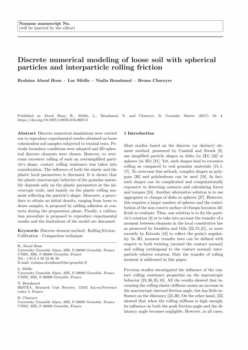
creases, the initial porosity after compaction increases

too, and the sample shows more and more an obvious

contractive behavior as shown in Figure 8. This hap-

pens up to a threshold adhesion value (here equal to

σA = 80 kPa or σAPc

=1), beyond which the numeri-

cal sample strongly collapses during the third step of

the compaction method leading to lower porosities and

more dilatant behavior (see the results for σAPc

=1.25 andσAPc

=2.5 in Figures 7 and 8). Figure 8 shows the triax-

ial compressions simulated from the accessible densities

reached by this method. It can be observed that re-

moving completely the adhesion during the compaction

phase is not enough to reach dense samples presenting

a strong dilatant behavior. For that, contacts need to

Fig. 6: Evolution of the porosity and the dimensionless

unbalanced force during the three steps of compaction.

be lubricated during the compaction phase by fixing a

low friction angle, as described for instance in [33], and

illustrated in Figures 7 and 8 for a lower values of the

contact friction angle during compaction. Hence, a large

range of initial density can be reached by assigning dur-

ing compaction either an artificial contact adhesion or

a reduced contact friction.

4 Modelling of the soil mechanical behaviour

In this section, a calibration procedure is defined and

then applied to reproduce the experimental data ob-

tained from drained triaxial compression tests with Pc =

200 kPa (i.e. constant effective confining stress). More-

over, to validate our model, it was tested with the data

obtained from: triaxial compression tests with differ-

ent confining pressures, undrained triaxial test (i.e. no

volume change) as well as constant deviator stress test

(constant q) [20].

4.1 Calibration process

After studying the influence of different parameters in-

corporated in our DEM model, a calibration procedure

based on the simulated response to a triaxial compres-

sion was defined as follows:

1. As the residual shear strength is independent of

the initial porosity and of the contact friction for

ϕc > 15◦, then ηr can be first calibrated by re-

producing the experimental residual friction angle

while ϕc is set arbitrarily (let’s say for instance 30◦


(a)

(b)

Fig. 7: Range of porosity reached after compaction for:

(a) introduction of contact adhesion σa during com-

paction (with (φc)comp=30 ◦), and (b) reduction of con-

tact friction angle, (φc)comp, during compaction.

as a first approximation of the contact friction be-

tween two silica particles). For this step, the numer-

ical sample may be compacted without the addition

of contact adhesion or contact lubrication in order

to start from a medium dense material.

2. Volumetric strain (i.e. dilatancy / contractancy) and

peak stress (if any) are approached as close as pos-

sible by fine tuning the initial sample density. To

get a looser material, adhesion is introduced during

the compaction phase, while contacts are lubricated

during the latter phase to reach a denser assembly,

as described in the previous section.

(a)

(b)

Fig. 8: Effect of adhesion, σA, during compaction, on

(a) the stress-strain response to a triaxial compression

and (b) porosity (case 4 in Table 1).

3. Contact friction angle ϕc is calibrated (if necessary)

to improve the reproduction of the volumetric strain

and the peak stress. Knowing that a change of ϕccan affect the initial porosity reached after the com-

paction phase, it may be necessary to reiterate steps

2 and 3 until a satisfying calibration of both the ini-

tial porosity and ϕc is achieved.

Calibration of elastic parameters, contact elastic mod-

ulus, Ec, and shear factor, αs, appears secondary to

plastic parameters (as long as they are beyond the stiff


limit), with respect to their effects on the macroscopic

mechanical behavior. They can be adjusted if neces-

sary to better reproduce the macroscopic initial Young

modulus and Poisson ratio as discussed in [23]. Rolling

stiffness, αr, is just kept close to the rigidity limit, not

lower to avoid any impact on plastic macroscopic prop-

erties, but not higher to avoid possible reduction of the

critical time step as discussed in section 2.2.

It is worth noting that this proposed calibration pro-

cedure stresses more on the rolling friction than on the

contact friction angle. Indeed, one can expect the con-

tact friction angle not to be very different for different

granular soils since grains are generally made with sim-

ilar constituents (silica and alumine), whereas particle

shapes, reflected by the rolling friction, may change a

lot and directly impact the soil mechanical behavior.

4.2 Validation on laboratory triaxial compression

paths

The calibration procedure is applied to calibrate the

numerical model on experimental data obtained from

drained triaxial compression tests on a Camargue sandy

soil. Laboratory triaxial compression results are pre-

sented in [20,2]. The triaxial tests were performed on

very loose Camargue sand samples prepared with an

initial (i.e. before isotropic compression) relative den-

sity of 20%. The particle size distribution of the nu-

merical model partially follows the one of the sand as

presented in Figure 9. It has been simplified by remov-

ing 3% of the largest particles and 3% of the smallest

ones to limit the total number of discrete elements andso to reduce the computational cost.

Fig. 9: The gradation curve of the Camargue sand.

The model has been calibrated from a drained triaxial

compression with a confining pressure, Pc = 200 kPa

(Figure 10), leading to the parameters shown in Ta-

ble 2.

(a)

(b)

Fig. 10: Comparison between experimental drained tri-

axial compression tests and DEM simulations on loose

Camargue sand. (a) deviator stress, (b) volumetric

strain.

When applied to compressions with different confining

pressures than the one used for calibration (Figure 10),

the model succeeded to describe the shear strength but

partially failed in reproducing quantitatively the depen-

dence of the volumetric strain on the confining pressure.

The important reduction of contractancy of the sand

obtained experimentally for Pc = 100 kPa, with respect


Pc Ec αs ϕc αr ηrσA (for com-paction only)

(kPa) (kPa) (deg) (kPa)

200 2 105 0.2 25 7.5 0.22 200

Table 2: Summary of the parameters calibrated on the loose Camargue sand.

to Pc = 200 kPa and 400 kPa, is underestimated by the

model.

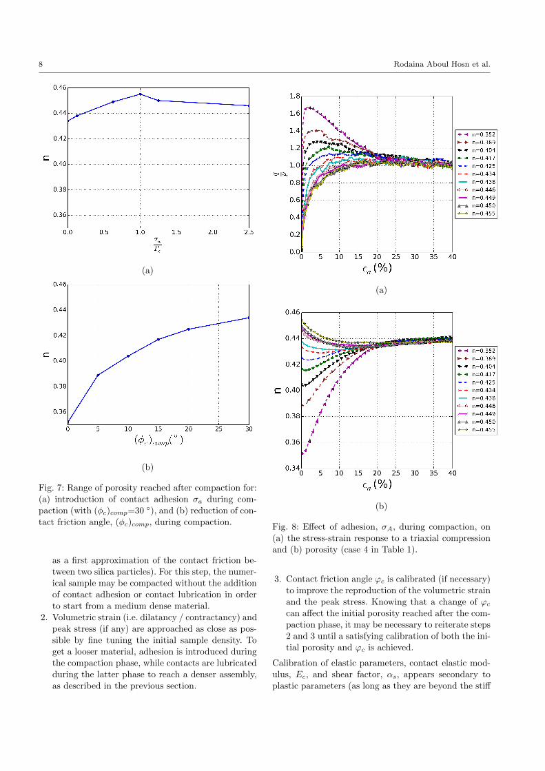
Responses of the calibrated model and of the sand sub-

jected to an undrained compression, after an initial

isotropic compression, Pc = 200 kPa, are compared in

Figure 11. The model exhibits sudden and total lique-

faction at very low axial strain which was not the case

experimentally for the sand, as if the ability of the nu-

merical model to contract was more important than for

the sandy sample. Responses were also compared to a

constant deviator stress loading path performed after

an initial drained compression. Stress and strain paths

are displayed in Figure 12. The numerical model cor-

rectly describes the stress state at failure occurrence but

predicts a much more contractant response than the ex-

perimental data. The constant shear drained path, such

as the q-constant path, lead to a reduction of the mean

pressure p. Consequently, the overestimation of contrac-

tancy along these loading paths is in agreement with the

results obtained from the drained compressions (Fig-

ure 10). In the latter case, we showed that the model

underestimates the reduction of contractancy with the

decrease of the mean pressure.

The observed difference of the dependency of volumet-

ric strain on mean pressure can be related to different

factors that differ between experimental and numerical

tests:

1. Difference of the compressibility behavior induced

by the isotropic compression: for the numerical sam-

ple, the relative variations of porosity after com-

paction when confining pressure is increased from

Pc = 100 kPa to 200 kPa, and up to Pc = 400

kPa, are -0.09 % and -0.81 % respectively, whereas

experimentally the sand sample presents a more im-

portant compressibility with relative porosity varia-

tions equal to -0.82 % and -2.22 % (always with re-

spect to the state for Pc=100 kPa). This difference

is particularly important in the range of confining

pressure 100 kPa- 200 kPa where the relative reduc-

tion of porosity for the numerical model is about 9

times smaller than what is found experimentally.

This may contribute to the discrepancy between

numerical and experimental volumetric strains ob-

served, especially for the compression at Pc = 100

kPa.

2. Different particle shapes: this is related to the abil-

ity for angular or elongated particles to untangle. A

reduction of the mean pressure, allowing more flex-

ibility for angular or elongated particles to rotate,

can promote their disentanglement, and thus a lower

contractive behavior. In addition, even without any

translation motion of particles, new contacts may be

formed with elongated particles in rotation, limiting

further compaction of the granular assembly. Such

mechanisms are not reproduced with the numerical

model made of spheres, even with the introduction

of a contact resistance to rolling, and apparently,

constitutes a limitation of the model.

5 Conclusion

This paper presented the DEM modeling of the soil

mechanical behaviors by using spherical particles and

contact rolling resistance. It was demonstrated that the

macroscopic behavior of the granular assembly mainly

depends, on one hand, on the initial packing density

and, on the other hand, on the model parameter fixingthe plastic rolling moment at contacts. Other parame-

ters as normal contact stiffness or contact friction angle

prove to play a secondary role (bearing in mind that the

contacts should be sufficiently stiff and based on a given

particle gradation). This is consistent with the fact that

the shear strength in cohesionless soil is more strongly

related to particle shape (presented here by the plastic

rolling moment) than to the inter-particle friction an-

gle, as shown previously by [10]. Moreover, it is greatly

affected, together with dilatancy, by the initial density.

Consequently, a new numerical method of compaction

was proposed, involving either the introduction of inter-

particle adhesion forces or the lubrication of contacts,

to reach a wide range of initial density of granular as-

semblies, from very loose to very dense. However, it was

shown that even if our model succeeds in reproducing

the experimental data, there are some limitations to be

taken into account related to the description of the de-

pendency of volumetric strains on the mean pressure.

This is due to the difference in the relative variation of


Fig. 11: Comparison between experimental and numer-

ical responses under undrained triaxial compression.

initial porosity after compaction between experimental

and numerical tests as well as due to the different par-

ticle shapes. Such marked differences may be partially

due to the very loose state of the tested sample.

Despite the latter limitation, one should keep in mind

the little number of parameters involved in such a model.

In total five parameters are involved, among which three

elastic parameters are secondary if sufficiently close to

the stiff limit, compared to a basic phenomenological

elasto-plastic constitutive relation (without any hard-

ening mechanisms) involving a minimum of four param-

eters (Young modulus, Poisson ratio, internal friction

angle, and dilatancy angle). Moreover, the dependency

of the dilatancy angle or the friction angle on the mean

pressure for such elasto-plastic constitutive relation re-

quires some additional empirical laws coming with ad-

ditional parameters.

Fig. 12: Comparison between experimental and numer-

ical responses under constant deviator stress loading

path just up to failure point.

Acknowledgements

The environment and support provided by the French

research group GDR MeGe 3176 is gratefully acknowl-

edged.

Laboratory 3SR is part of the LabEx Tec 21 (Investisse-

ments d’Avenir - grant agreement n◦ANR-11-LABX-

0030)

Appendix

Let ~u, ~θ define small movements of a particle relative to an ini-tially stable configuration in which the total force and torqueon the particle are ~F = ~T = ~0. If the particle is involved in Nccontacts and every contact remains elastic (worst case), the


new force and torque induced by ~u and ~θ can be expressed asfollows, in which the translational and the rotational degreesof freedom are uncoupled (this uncoupling assumption is alsofound in [12]): (Note that since ~F = ~T = ~0, then we can write∆~F = ~F and ∆~T = ~T ):

~F ' −

(Nc∑c=1

(Kn −Ks)(~n⊗ ~n) +KsI

)~u (12)

~T ' −r2Nc∑c=1

Ks(I− ~n⊗ ~n)~θ (13)

I being the inertia tensor of the particle and r its radius.These forces are given by neglecting the rotational term inequation 12 and the translational term in equation 13.

If contact moments ( ~Mr and ~Mtw) are present, the moments(initially null) induced at each contact (remaining elastic) by~u and ~θ are:

~Mtw = −Ktw(~θ · ~n)~n

= −Ktw(~n⊗ ~n)~θ, (14)

~Mr = −Kr(~θ − (~θ · ~n)~n)

= −Kr(I− ~n⊗ ~n)~θ. (15)

where Kr and Ktw are the rolling and twisting stiffnesses, re-spectively. Note that, in our study, only the rolling momentwas taken into consideration. However, for generalization, weadded the twisting moment here.

Adding these contributions (eq. 14 and 15) to the global ro-tational stiffness (eq. 13) yields

~T ' −Nc∑c=1

{r2Ks(I− ~n⊗ ~n) +Ktw~n⊗ ~n+Kr(I− ~n⊗ ~n)}~θ (16)

The uncoupled equations of motion for the particle can beexpressed as:

~u = −Ku

M~u, (17)

~θ = −

Kθ

J~θ, (18)

where Ku and Kθ are the tensors defined by equations 12and 16 respectively, M is the mass of the particle, and J isthe moment of inertia (equal to 2

5r2M for a sphere).

KuM

and KθJ

are symmetric positive definite tensors from whichsix eigen values can be calculated, corresponding to six nat-ural frequencies of the particle. The explicit centered finitedifference scheme is stable for the above equations - for asingle particle b - as long as ∆t is less than 2/

√λbmax, λbmax

being the maximum eigenvalue of the particle.

A multi-body system as a whole may have natural oscilla-tion modes combining the motion of multiple particles, withfrequencies higher than the maximum frequency found for in-dividual particles. An accurate determination of the criticaltimestep would thus need to consider the stiffness matrix of

the system as a whole where the motion of two particles incontact would be included. For Nb particles it would lead to amatrix of size (6Nb)2 from which eigenvalues would have to beextracted. It can be avoided by remarking that this large as-sembled matrix would have every contact stiffness appearingtwice in each row (once in the diagonal term and once in thecolumn whose index corresponds to the other particle formingthe contact). Since the absolute row-sum of the componentscan be used as an upper bound of the maximum eigenvalue(Perron-Froebenius theorem [3]) an upper bound is obtainedsimply by multiplying every stiffness by two when calculat-ing the frequencies of one single particle. Equivalently, wecan keep the stiffness unchanged and define the upper boundusing the eigenvalues associated to individual particles as

λmax < 2 maxb

(λbmax). (19)

[13] suggested a similar inequality without proof. Finally, asufficient condition of stability is:

∆t <

√2

maxb(λbmax). (20)

The equations of motion for a particle, 17 and 18, can bewritten in a simplified way considering the following assump-tions:

1. all spheres are identical (same size and same inertia)2. all contacts have the same stiffness values3. the stiffness tensors, defined by equations 12 and 16, are

isotropic.

We note also that Kr = αrnr2Kn and K − tw = αtwr2Kn.Then the uncoupled equations of motion read:

~u = −NcKn(1 + 2αs)

M~u, (21)

~θ = −

NcKn(5αs + 5αrn + 2.5αtw)

M~θ (22)

References

1. J.P Bardet. Observations on the effects of particle rota-tions on the failure of idealized granular materials. Me-

chanics of Materials, 18(2):159–182, 1994.2. N. Benahmed, T.K. Nguyen, P.Y. Hicher, and M. Nicolas.

An experimental investigation into the effects of low plas-tic fines content on the behaviour of sand/silt mixtures.European Journal of environmental and civil engineering,19(1):109–128, 2015.

3. A. Brauer and A.C. Mewborn. The greatest distancebetween two characteristic roots of a matrix. Duke Math.J., 26(4):653–661, 1959.

4. F. Calvetti, G. Viggiani, and C. Tamagnini. A numeri-cal investigation of the incremental behavior of granularsoils. Riv.Ital.Geotech, 3:11–29, 2003.

5. B. Chareyre, L. Briancon, and P. Villard. Theoreticalversus experimental modeling of the anchorage capacityof geotextiles in trenches. Geosynth. Int., 9(2):97–123,2002.

6. B. Chareyre and P. Villard. Dynamic spar elements anddiscrete element methods in two dimensions for the mod-eling of soil-inclusion problems. Journal of Engineering

Mechanics, 131(7):689–698, 2005.


7. G. Combe. Origines geometrique du comportement quasi-statique des assemblages granulaires denses: etude par simu-

lations numeriques. PhD thesis, Ecole nationale des pontset chaussees, 2001.

8. P.A. Cundall and O.D.L. Strack. A discrete numericalmodel for granular assemblies. Geotechnique, 29(1):47–65, 1979.

9. F. da Cruz, S. Emam, M. Prochnow, J-N. Roux, andF. Chevoir. Rheophysics of dense granular materials: Dis-crete simulation of plane shear flows. Physical review E,72, 021309, 2005.

10. N. Estrada, E. Azema, F. Radjaı, and A. Taboada. Com-parison of the effects of rolling resistance and angular-ity in sheared granular media. Powder and grains, hal-00842799:891–894, 2013.

11. F. Gilabert, J.-N. Roux, and A. Castellanos. Computersimulation of model cohesive powders: Influence of assem-bling procedure and contact laws on low consolidationstates. Physical Review E, 75, 011303, 2007.

12. Itasca Consulting Group. PFC3D theory and backgroundmanual, version 3.0, 2003.

13. R. Hart, P.A. Cundall, and J. Lemos. Formulation ofa three-dimensional distinct element model-part II. me-chanical calculations for motion and interaction of a sys-tem composed of many polyhedral blocks. International

Journal of Rock Mechanics and Mining Sciences & Geome-chanics Abstracts, 25(3):117–125, 1988.

14. X. Huang, K.J. Hanley, C. O’Sullivan, and C.K. Kwok.Exploring the influence of interparticle friction on criticalstate behavior using DEM. Int. J. Numer. Anal. Meth.Geomech, 38(12):1276–1297, 2014.

15. K. Iwashita and M. Oda. Micro-deformation mecha-nism of shear banding process based on modified distinctelement method. Powder Technology, 109(1-3):192–205,2000.

16. M.J. Jiang, J.M. Konrad, and S. Leroueil. An effi-cient technique for generating homogeneous specimensfor DEM studies. Computers and Geotechnics, 30(7):579–597, 2003.

17. J. Kozicki and J. Tejchman. Numerical simulations ofsand behaviour using DEM with two different descrip-tions of grain roughness. In II International Conference on

Particle-based Methods – Fundamentals and Applications,Particles, 2011.

18. J. Kozicki, J. Tejchman, and D. Lesniewska. Studyof some micro-structural phenomena in granular shearzones. In Powder and Grains, AIP Conference proceeding,volume 1542, 2013.

19. S.J. Lee, Y.M.A. Hashash, and E.G. Nezami. Simulationof triaxial compression tests with polyhedral discrete el-ements. Computers and Geotechnics, 43:92–100, 2012.

20. T.K. Nguyen. Etude experimentale du comportement insta-ble d’un sable silteux: Application aux digues de protection.PhD thesis, Universite d’Aix-Marseille, 2014.

21. M. Oda and K. Iwashita. Study on couple stress and shearband development in granular media based on numericalsimulation analyses. International Journal of EngineeringSciences, 38(15):1713–1740, 2000.

22. M. Oda, J. Konishi, and S. Nemat-Nasser. Experimentalmicromechanical evaluation of strength of granular ma-terials: Effects of particle rolling. Mechanics of Materials,1(4):269–283, 1982.

23. J.-P. Plassiard, N. Belheine, and F.-V. Donze. A sphericaldiscrete element model: calibration procedure and incre-mental response. Granular Matter, 11(5):293–306, 2009.

24. F. Radjaı and F. Dubois. Discrete-element modeling ofgranular materials. ISTE Ltd and John Wiley & Sons,2011.

25. J-N. Roux and F. Chevoir. Discrete numerical simula-tion and the mechanical behavior of granular materials.Bulletin des laboratoires des ponts et chaussees – n 254,2005.

26. J-N. Roux and G. Combe. How granular materials de-form in quasistatic conditions. In IUTAM-ISIMM Sym-

posium on Mathematical Modeling and Physical Instancesof Granular Flow. AIP publishing., volume 1227(1), pages260–270, 2010.

27. C. Salot, P. Gotteland, and P. Villard. Influence of rela-tive density on granular materials behavior: DEM simu-lations of triaxial tests. Granular Matter, 11(4):221–236,2009.

28. L. Scholtes, B. Chareyre, F. Nicot, and F. Darve. Mi-cromechanics of granular materials with capillary ef-fects. International Journal of Engineering Science, 47(11-12):1460–1471, 2009.

29. B. Suhr and K. Six. On the effect of stress dependentinterparticle friction in direct shear tests. Powder Tech-

nology, 294:211–220, 2016.30. K. Szarf, G. Combe, and P. Villard. Polygons vs. clumps

of discs: A numerical study of the influence of grain shapeon the mechanical behaviour of granular materials. Pow-

der Technology, 208(2):279–288, 2011.31. C. Thornton. Numerical simulations of deviatoric shear

deformation of granular media. Geotechnique, 50(1):43–53, 2000.

32. JM. Ting, BT. Corkum, CR. Kauffman, and C. Greco.Discrete numerical model for soil mechanics. J GeotechEng, 115(3):379–398, 1989.

33. A.-T. Tong, E. Catalano, and B. Chareyre. Pore-scaleflow simulations: Model predictions compared with ex-periments on bi-dispersed granular assemblies. Oil & Gas

Science and Technology – Revue IFP Energies nouvelles,67(5):743–752, 2012.

34. V. Smilauer et al. Yade Documentation 2nd ed. The YadeProject, 2015. http://yade-dem.org/doc/.

35. X. Wang and Li J. Simulation of triaxial response of gran-ular materials by modified DEM. Science China: Physics,

Mechanics and Astronomy., 57(12):2297–2308, 2014.36. L. Widulinski, J. Kozicki, and J. Tejchman. Numeri-

cal simulations of triaxial test with sand using DEM.Archives of Hydro-Engineering and Environmental Mechan-ics, 56(3-4):149–171, 2009.

Documents

Discrete numerical modeling of loose soil with spherical