Direct Transpiration and Naphthalene Uptake Rates for a Hybrid Poplar Based Phytoremediation System

Michael J. Nelson

Thesis submitted to the faculty of the Virginia Polytechnic Institute and State University in partial fulfillment of the requirements for the degree of

Master of Science

In Environmental Engineering

Committee: Mark A. Widdowson, Chairman

John T. Novak Linsey Marr

February 10, 2005 Blacksburg, Virginia

Keywords: Transpiration, Evapotranspiration, Phytoremediation, Hybrid Poplar,

Naphthalene, Plant Uptake

Copyright 2005, Michael J. Nelson

Direct Transpiration and Naphthalene Uptake Rates for Hybrid Poplar Based Phytoremediation System

Michael J. Nelson

ABSTRACT

Direct transpiration rates and plant uptake of naphthalene by a hybrid poplar

phytoremediation system located in Oneida, Tennessee were determined using hydrologic

and groundwater concentration data. Water table recession analysis techniques were

employed to determine direct transpiration rates from the saturated zone of the shallow,

unconfined aquifer underlying the site. Direct transpiration rates varied over the growing

season (late March to mid-October), with a maximum and mean daily direct transpiration

of 0.0100 and 0.0048 feet/day, respectively. During 2004, the maximum direct

transpiration rate was observed in May, and rates declined starting in June due to an

associated decline in the water table. A technique was developed to estimate the

volumetric transpiration rate of each tree based on the breast-height diameters and

seasonally variable direct transpiration rates. During peak transpiration, the larger trees

at the study site were estimated to directly transpire 4 to 13 gallons per day per tree.

Plant uptake rates of naphthalene were estimated by superimposing spatial data

(volumetric transpiration rates and naphthalene concentration in groundwater). The mass

loss rate of naphthalene from the aquifer as a result of plant uptake during July 2004 was

335 mg/day which only represents 0.117% of the aqueous mass plume. Monthly

groundwater profiles showed a decrease of the saturated thickness beneath the system of

hybrid poplars between the dormant and active season. This study suggests direct

transpiration rates and plant uptake of naphthalene are dependent on variables including

climatic parameters, magnitude of the saturated thickness, and the concentration of

naphthalene in groundwater.

iii

TABLE OF CONTENTS

1 INTRODUCTION ...................................................................................................... 1

1.1 Phytoremediation Overview ............................................................................... 1 1.2 Objectives ........................................................................................................... 3 1.3 Approach............................................................................................................. 3

2 LITERATURE REVIEW ........................................................................................... 5

2.1 Transpiration and Evapotranspiration................................................................. 5 2.2 Water Table Fluctuations in an Unconfined Aquifer.......................................... 8

2.2.1 Water Table Fluctuation Due to Recharge & Air Entrapment ................... 8 2.2.2 Water Table Fluctuations Due to Evapotranspiration/Transpiration .......... 9 2.2.3 Water Table Fluctuations Due to Atmospheric Pressure Changes ........... 10

2.3 Hybrid Poplar Trees and Water Use ................................................................. 10 2.4 Relationship between Transpiration and Tree Size .......................................... 12 2.5 Phytoremediation and Plant Uptake of Contaminants ...................................... 13

3 SITE DESCRIPTION ............................................................................................... 15

3.1 Site History ....................................................................................................... 15 3.2 Site Hydrology & Hydrogeology...................................................................... 15 3.3 Contaminant Location....................................................................................... 17

4 MATERIALS AND METHODS.............................................................................. 18

4.1 Phytoremediation System & Monitoring Location Overview.......................... 18 4.2 Field Methods ................................................................................................... 21

4.2.1 Groundwater Level Monitoring ................................................................ 21 4.2.2 Hydrologic Monitoring ............................................................................. 24 4.2.3 Tree Growth Monitoring........................................................................... 24

4.3 Data Techniques to Quantify Transpiration Rates............................................ 25 4.3.1 Groundwater Recession Comparison Method .......................................... 26 4.3.2 White’s Equation ...................................................................................... 28

4.4 Determination of Direct Transpiration Flow Rates .......................................... 29 4.5 Determination of the Direct Uptake of Naphthalene ........................................ 34

4.5.1 Naphthalene Concentration Data .............................................................. 35 4.5.2 Spatial Distribution of Naphthalene.......................................................... 36 4.5.3 Calculation of Mass Removal of Naphthalene via Plant Uptake.............. 37 4.5.4 Plot of Discrete Water Level Measurements ............................................ 38 4.5.5 Groundwater Contours.............................................................................. 38 4.5.6 Water Table Profiles ................................................................................. 39

5 RESULTS AND DISCUSSION............................................................................... 41

5.1 Summary of Data Utilized for this Study ......................................................... 41 5.1.1 Oneida Rainfall Data................................................................................. 41 5.1.2 Continuously Recorded Water Table Elevations...................................... 44 5.1.3 Discrete Water Level Data........................................................................ 47 5.1.4 Tree Growth .............................................................................................. 49

5.2 Quantification of Direct Transpiration Rates.................................................... 51 5.2.1 Results of Groundwater Recession Comparison Method ......................... 51

iv

5.2.2 Results of White’s Equation ..................................................................... 54 5.2.3 Saturated Thickness Estimation................................................................ 55 5.2.4 Time Trend of Direct Transpiration Rates and Saturated Thickness........ 56 5.2.5 Comparison of Direct Transpiration Rates to Past Results....................... 58 5.2.6 Comparison of Direct Transpiration at Oneida to Other Sites.................. 61

5.3 Estimation of Volumetric Direct Transpiration Rates ...................................... 61 5.3.1 Results of Individual Tree Volumetric Transpiration Rates ..................... 61 5.3.2 Variation of the k-value ............................................................................ 62 5.3.3 Application of the k-value to Study Site Poplar Trees ............................. 66 5.3.4 Comparison of Volumetric Direct Transpiration to Past Results ............. 67 5.3.5 Comparison of Volumetric Direct Transpiration at Oneida to Other Sites 67

5.4 Plant Uptake Rates of Naphthalene .................................................................. 68 5.4.1 Time Trend of Groundwater Concentrations of Naphthalene .................. 68 5.4.2 Mass Rate of Plant Uptake of Naphthalene .............................................. 77 5.4.3 Estimated Time Trend of Plant Uptake of Naphthalene for Oneida Site . 78

5.5 Plans and Profiles of Water Table Elevation Data............................................ 79 5.5.1 Cone of Depression................................................................................... 79 5.5.2 Change of Hydraulic Profile over Time.................................................... 80

6 SUMMARY AND CONCLUSIONS ....................................................................... 84

6.1 Summary of Findings........................................................................................ 84 6.1.1 Quantification of Direct Transpiration Rates............................................ 84 6.1.2 Estimation of Volumetric Transpiration ................................................... 85 6.1.3 Quantification of Naphthalene Removal via Direct Transpiration ........... 87

6.2 Conclusions....................................................................................................... 87 6.3 Future Considerations ....................................................................................... 89

7 REFERENCES ......................................................................................................... 90

Appendix A Water Table Elevation and Rainfall Data…………………………..........93

Appendix B Groundwater Recession Comparisons…………………………………...99

Appendix C Water Table Contours and Profiles……………………………………..124

Appendix D Tree Data………………………………………………………………..149

Appendix E Direct Transpiration Distribution Plots…………………………………168

Appendix F Naphthalene Concentration Contours…………………………………..194

VITA……………………………………………………………………………………214

v

LIST OF FIGURES: Figure 2.1 Example of diurnal fluctuations in shallow observation wells in Canada

(Freeze & Cherry, 1979 p.231). .................................................................................. 6

Figure 2.2 Hybrid poplar tree, Populus deltoides x Populus trichocarpa ........................ 11

Figure 3.1 Oneida Tie Yard Site Plan (ARCADIS Geraghty & Miller, 2000)................. 17

Figure 4.1 2004 Site Plan of Oneida phytoremediation site. ............................................ 19

Figure 4.2 Monitoring System for Oneida Phytoremediation Site ................................... 21

Figure 4.3 Schematic of piezometer/monitoring well illustrating top of casing (TOC),

water table (WT), base of transducer (BOT), transducer depth (TD)....................... 22

Figure 4.4 Locations and identification numbers of hybrid poplars as of June 2004....... 25

Figure 4.5 Example of water table recession comparison between two dormant season

durations.................................................................................................................... 26

Figure 4.6 Groundwater Recession Comparison: dormant versus active durations. ........ 28

Figure 4.7 Example of White’s Equation applied to August, 2004 MW6 data. ............... 29

Figure 4.8 Division of phytoremediation system into 10 x 10 foot cells.......................... 30

Figure 4.9 Representative 900 square-foot area around each observation point. ............. 31

Figure 4.10 Representative 2500 square-foot area around each observation point. ......... 31

Figure 4.11 Range of per tree direct transpiration rates around MW6 for May 6, 2004

duration. .................................................................................................................... 34

Figure 4.12 Location of multilevel samplers at the Oneida phytoremediation site. ......... 35

Figure 4.13 Average naphthalene concentrations derived from the upper two ports of

multilevel samplers at the Oneida phytoremediation site in June 1999.................... 36

Figure 4.14 Oneida phytoremediation system naphthalene concentration contours

interpolated from point measurements taken in June 1999 ...................................... 37

Figure 4.15 Groundwater contours interpolated from discrete water level measurements

taken on March 6, 2004. ........................................................................................... 39

Figure 4.16 Water table profile and groundwater contours for March 6, 2004. The profile

line with station labels 0+00 to 2+63 intersects P3 and P9. ..................................... 40

Figure 5.1 Comparison of monthly rainfall totals from 1999 to 2004 and 100-year

average. ..................................................................................................................... 42

Figure 5.2 Rainfall recorded by weather station at phytoremediation site, 2004. ............ 44

vi

Figure 5.3 Continuous water table elevation and rainfall data from 2004........................ 45

Figure 5.4Continuous water table elevation and rainfall data, 2000-2003 ....................... 45

Figure 5.5 Running average of continuous water table elevation and daily rainfall data

from 2004 and 2001. ................................................................................................. 47

Figure 5.6 Hybrid poplar growth and survival at Oneida site between 1999 and 2004 ... 49

Figure 5.7 Range of tree diameters found at Oneida site (Total = 693), June 2004......... 50

Figure 5.8 Groundwater Recession Comparison method series for MW6. ...................... 52

Figure 5.9 White’s Equation applied to diurnal data from May and August 2004........... 54

Figure 5.10 Time trend of 2004 direct transpiration rates and average saturated thickness

(H) for observation points MW6, P4, and P25. ........................................................ 56

Figure 5.11 September 23, 2004 TDT comparison. ........................................................... 58

Figure 5.12 2004 TDT versus 1999 TDT............................................................................. 58

Figure 5.13 Comparison of 2004 TDT to 1999 ET ............................................................ 59

Figure 5.14 Series of per tree volumetric direct transpiration versus tree diameter plots of

trees within 900 ft2 area surrounding MW6.............................................................. 62

Figure 5.15 Time trend of k-values from all observation points during 2004.................. 65

Figure 5.16 Distribution of volumetric direct transpiration over time based on DBH. .... 66

Figure 5.17 Concentrations determined by averaging concentrations measured from the

top 2 ports of each multilevel sampler. ..................................................................... 69

Figure 5.18 Concentrations measured from top port of each multilevel samplers. .......... 70

Figure 5.19 Comparison of the average of the top two ports versus the top port only..... 71

Figure 5.20 Dormant season naphthalene mass compared with average saturated

thickness.................................................................................................................... 72

Figure 5.21 Active season naphthalene mass compared with average saturated thickness.

................................................................................................................................... 73

Figure 5.22 Time trend of dormant season naphthalene mass and yearly rainfall. .......... 75

Figure 5.23 Time trend of dormant season naphthalene mass and yearly rainfall. .......... 75

Figure 5.24 Mass of Naphthalene versus saturated thickness, H...................................... 76

Figure 5.25 Mass of naphthalene versus yearly rainfall totals.......................................... 76

Figure 5.26 Interpolation of k-value for July 6, 2004....................................................... 77

Figure 5.27 Time trend of plant uptake assuming a “typical” mid-summer k-value........ 78

vii

Figure 5.28 Plan view of water table contours for data measured on July 6, 2004. ......... 80

Figure 5.29 Comparison of water table profiles for March, April, and May.................... 81

Figure 5.30 Comparison of water table profiles for June, July, and August. ................... 82

Figure 5.31 Water table profiles for September and October. .......................................... 83

LIST OF TABLES: Table 3.1 Average Climatological Observations for Oneida, TN .................................... 16

Table 4.1 Piezometer and monitoring well construction summary. ................................. 20

Table 4.2 Installation measurements for each pressure transducer................................... 23

Table 4.3 Sample calculation for estimating the volumetric transpiration rates of trees

within a nine-cell (900 ft2) area surrounding the observation point (MW6). ........... 33

Table 5.1 Precipitation record for Oneida, Tennessee. Rain gauge located at Oneida

wastewater treatment plant (WWTP). Data Source: National Climatic Data Center.

................................................................................................................................... 42

Table 5.2 Discrete water level measurement results for 2004. ......................................... 48

Table 5.3 Direct transpiration rates, TDT (feet/day) calculated for 2004 from observation

points MW6, P4, and P25. ........................................................................................ 53

Table 5.4 Results of White’s Equation at Oneida phytoremediation site, 2004. .............. 54

Table 5.5 Saturated thicknesses at MW6, P4, and P25 at varying points in time............. 55

Table 5.6 Tabulated k-values resulting from the application of direct transpiration rates to

trees within representative areas surrounding observation points MW6, P4, and P25.

................................................................................................................................... 63

Table 5.7 Number of trees per square foot within representative areas surrounding each

observation point....................................................................................................... 64

1

1 INTRODUCTION

1.1 Phytoremediation Overview

Remediation of contaminated soil and groundwater has undergone significant

improvements since the introduction of conventional pump-and-treat. Phytoremediation

is an innovative in-situ technique that utilizes plants for enhancing the attenuation rate of

contaminated soil and groundwater (U.S. EPA, 2000). An array of mechanisms is

employed to remediate various contaminants from subsurface media depending on the

contamination and type of plants (Pivetz, 2001).

Studies indicate that phytoremediation influences the fate of contaminants found

in soil, sediments, and groundwater by degradation, removal, and immobilization (Pivetz,

2001). Though effective, these remediation mechanisms tend to occur simultaneously,

making them difficult to differentiate. While immobilization (removing the means for

transport) can in part be accomplished utilizing plants which reduce recharge via

interception, hydraulic control can best be accomplished by phreatophytic consumption

because it slows the migration of contaminant plumes by providing a sink for

groundwater flow (U.S. EPA, 2000). For a phytoremediation system, phreatophytic

consumption use is the single-most influential factor on hydraulic control (Vose et al,

2003).

Plant water use is driven by evaporative loss, or evapotranspiration.

Evapotranspiration from a land area can be divided into two components:

1) transpiration of water from the subsurface through plants leaves, and 2) the

evaporation of water from soils and water bodies (Viessman & Lewis, 2003).

Transpiration is the uptake of water by plants through soil, roots, and stems followed by

the subsequent release to the atmosphere via evaporation across the leaf surface (Noggle,

1976). Water loss from an aquifer is best described by direct transpiration since it does

not include water loss from the land surface. Direct transpiration refers to transpiration

which removes groundwater directly from the saturated zone of an aquifer. Success of a

phytoremediation system is dependent on transpiration because plants must consume

enough groundwater to influence the fate of subsurface contaminants (Vose et al, 2003).

2

Transpiration rates are influenced by a variety of factors including climate, soil-

water availability, and time of season (Hopkins et al, 2004). Transpiration is a seasonal

process which occurs during spring and summer, or when the trees are leafed (Fitter et al,

1981). During fall and winter trees are not active and the transpiration process becomes

dormant.

Since plant water use is significant to the success of a phytoremediation system to

control groundwater flow, it is desirable to utilize a plant that has a large capacity for

transpiration. Due to their high water use, it has become a common practice to use

phreatophytes for phytoremediation. Phreatophytes are deep-rooted plants that seek

water in the saturated zone (Jordahl et al, 1996). A commonly used phreatophyte is the

hybrid poplar. Long-lived, perennial, and tolerant, hybrid poplars utilize copious

amounts of groundwater drawing from aquifers at depths upwards of fifteen feet (Freeze

& Cherry, 1979; Viessman & Lewis, 2003). A stand of poplar trees can create a

significant groundwater sink during the growing season, with the potential of inducing

groundwater flow towards the center of the poplar grove (Schneider, 2000).

Plant uptake is another important phytoremediation mechanism which refers to

the ability of plants to remove contaminants from an aquifer through transpiration. The

fate of contaminants interacting with a plant is dependent on the physical properties of

the contaminant and the type of plant. For instance, phytoextraction refers to the uptake

and accumulation of metals by plants via transpiration (Schnoor, 2002).

Phytovolatilization refers to the transport of volatile organic compounds (VOCs) from the

subsurface to the atmosphere via plant transpiration (U.S. EPA, 2000). Studies show that

hybrid poplars are capable of removing VOCs from contaminated aquifers and

discharging them through tree tissue into the atmosphere as a gaseous product

(Schneider, 2000). The uptake and subsequent metabolism of organic contaminants from

the subsurface is known as phytotransformation (Schnoor, 2002).

A phytoremediation project at Oneida, Tennessee has been underway for several

years. At its inception in 1997, 1,036 hybrid poplar trees were planted as a long-term

solution to hydraulically contain and remediate creosote-based contaminants in-situ.

Groundwater level monitoring at the Oneida site has provided hydrologic data indicating

the poplar trees directly transpire measurable amounts of water from the saturated zone of

3

the underlying shallow, unconfined aquifer (Panhorst, 2000). Recent tree tissue analysis

in conjunction with measurement of PAH concentrations in groundwater indicates poplar

trees are extracting and volatilizing contaminant mass from the subsurface (R. Anderson,

personal communication). The combination of these data indicates the phytoremediation

system at Oneida influences both plume migration and reduction of polycyclic aromatic

hydrocarbon (PAH) concentrations (Widdowson et al, in press).

1.2 Objectives

Two principal remedial goals at the Oneida phytoremediation site were to use the

system of poplar trees to hydraulically control the contaminant plume in the shallow

aquifer and to reduce the concentration of PAH compounds. The objectives of this study

were: 1) quantify the rate of groundwater directly transpired from the saturated zone

(TDT) using hydrologic data, 2) estimate volumetric direct transpiration rates across the

site on a per tree basis (QTDT), and 3) quantify the naphthalene mass removal rate by the

system of poplar trees.

1.3 Approach

The quantification of direct transpiration from the saturated zone of the aquifer

underlying the Oneida site is based on long-term hydrological and groundwater level

monitoring. Utilizing continuous water table elevation data within the phytoremediation

system, groundwater recession trends are established and used to calculate direct

transpiration via two techniques: 1) Groundwater Recession Comparison method and (2)

White’s Equation. Each of these methods results in a rate of direct transpiration in units

of feet/day.

Upon calculating direct transpiration in feet/day, the values are converted to

volumetric flowrate by multiplying by the land surface area. This value is then

distributed among the poplar trees growing within the land area, taking into account tree

mass. This in turn provides an estimate of the volumetric rate of direct transpiration on a

per tree basis.

The final step of this analysis is to spatially correlate the per tree volumetric

transpiration rates to concentration data of the contaminated plume. The volumetric rate

4

of direct transpiration for each tree is then multiplied by the local naphthalene

concentration and the Transpiration Stream Concentration Factor (TSCF) to quantify the

mass of contaminants leaving the aquifer via plant uptake.

5

2 LITERATURE REVIEW

2.1 Transpiration and Evapotranspiration

Transpiration is the evaporation of water from plant leaves (Fitter et al, 1981).

Transpiration primarily occurs at the leaf surface while the stomata are open for the

passage for CO2 and O2 during photosynthesis (Noggle, 1976). Also termed ‘active

transpiration,’ it is the component of water lost from the subsurface through live plants

(Mieresonne et al, 1999). Transpiration is influenced by the following factors: climate

(precipitation, temperature, vapor pressure, solar radiation, wind speed, humidity, and

barometric pressure), soil water availability, groundwater depth, leaf area, stomatal

functions, root mass and distribution, and aquifer parameters (Hopkins et al, 2004).

Transpiration is measured by both direct and indirect methods. Sap flow analysis,

widely considered a direct measurement of tree transpiration, is a determination of the

rate of water movement through trees from both the vadose zone and the saturated zone.

Sap flow is estimated by measuring the amount of heat which is transferred vertically in

the trees xylem due to upward water flow and multiplying the measured rate by some

scaling factor to determine the rate of transpiration (Kjelgaard, 1996). Single tree

quantifications of transpiration are extrapolated to estimate the water use of entire tree

stands (Schiller et al, 2001).

An older, less direct method for estimating transpiration resulted from water table

fluctuation analysis conducted by W.N. White in the early 1930s. Located in the arid

Escalante Valley of Utah, White monitored ground water levels and observed diurnal

water table fluctuations. White observed that during the day the water table fell while

after sunset the water table would begin to get higher again until the next morning when

the sun began to rise. Overall, White observed that the net change in groundwater levels

were lower than the day before. White attributed this diurnal pattern and water loss to

phreatophytic consumption. He concluded that during the day, when the tree stomata

were open, the water table fell. At night, when the stomata closed, the process of

transpiration halted until the next day. Analyzing the water table level data, White

6

developed an equation for estimating transpiration based on the slopes of diurnal water

table fluctuations (White, 1932).

Figure 2.1 Example of diurnal fluctuations in shallow observation wells in Canada

(Freeze & Cherry, 1979 p.231).

White explained his equation, “The total quantity of groundwater withdrawn by

transpiration and evaporation during the 24-hour period can then be determined by the

formula q = y(24r ± s), in which q is the depth of water withdrawn per 24 hours, in

inches, y is the specific yield of the soil in which the daily fluctuation of the water table

takes place, r is the hourly rate of rise of the water table from midnight to 4 a.m., in

inches, and s is the net fall or rise of the water table during the 24-hour period, in inches.

In field experiments the quantities on the right hand side of the formula except specific

yield can be readily determined from the automatic records of water-table fluctuation”

(1932). White also researched the effect of direct evaporation on water table decline. He

concluded that when the depth of the water table was beyond two feet from the land

surface, evaporative influence on the water table was almost negligible (White, W.N.,

1932). Therefore, according to White, diurnal fluctuations of the water table which is

greater than 2 feet below the land surface can be attributed to transpiration.

Transpiration is a seasonal process which is dependent on the condition of the

plant and meteorological conditions (Fitter et al, 1981). White (1932) observed that

diurnal water fluctuations began at first leaf in the spring and declined with defoliation

7

until all leaves had eventually dropped. The start and end of a typical growing season is

dependent on geographic location, elevation, and weather patterns.

Evapotranspiration (ET) is the combination of evaporation from soil surfaces,

evaporation of intercepted precipitation, and transpiration from the soil by plants (Freeze

and Cherry, 1979). Many researchers object to the term evapotranspiration and refer to

all processes of vapor transfer to the atmosphere from all surfaces as evaporation

(Monteith, 1973). Evapotranspiration is driven by the same parameters as transpiration;

however ET is used to describe the bulk amount of water evaporated from an area which

includes both bare soils and vegetation. In a water budget, ET typically has units of

length (vertical drawdown) per time and generally encompasses a large land area.

Evapotranspiration is measured by a variety of methods which utilize various

spatial and meteorological parameters. The Penman-Monteith (PM) method is an energy

balance based on vapor pressure, net radiation, air temperature and soil heat flux

(Monteith, 1965). The PM method is a popular way for determining ET, though

parameters are often estimated. The eddy covariance (EC) method is used to directly

measure fluxes between the land surface and the atmospheric surface layer whose

differences can be used to estimate values of evapotranspiration representing large areas

(Garratt, 1984). Moisture fluxes within the lower reaches of the atmosphere are

calculated and used to estimate ET. The Thornthwaite Method (TM) is based on air

temperature, latitude, and season (Thornthwaite, 1948). This method emphasizes

meteorological controls and ignores soil moisture changes. Since the availability of soil

water is unaccounted for, the Thornthwaite method results in an estimation of the

potential evapotranspiration (PET) of a large area.

Evapotranspiration measurement methods do not provide or take into account

source water (aka: groundwater). Since trees often utilize rainwater stored in the vadose

zone, measured evapotranspiration rates do not correlate well with fluctuations of

groundwater levels (Davis and Peck, 1986; Cramer, 1999). For this reason, transpiration

is the most applicable process for determining the effectiveness of a phytoremediation

system since the plants must transpire enough water from the subsurface to uptake

contaminants (Vose et al, 2003). The quantification of transpiration requires

8

comprehensive evaluation of site specific data pertaining to groundwater fluctuations,

climate, and soil water availability (Vose et al, 2003).

2.2 Water Table Fluctuations in an Unconfined Aquifer

Groundwater level monitoring is an important component of many hydrologic

investigations. Fluctuations observed in wells and piezometers are good indicators of

recharge, yield, and consumptive water use, but may be skewed by other outside

influences (air entrapment, bank storage near streams, tidal effects near oceans, pumping,

artificial recharge, geotechnical drainage) (Freeze and Cherry, 1979). The elevation of

the groundwater table at a particular location rises and falls for a variety of reasons

including recharge, evapotranspiration, barometric pressure influences, and air

entrapment. The two most significant causes of water table fluctuations are recharge and

evapotranspiration (Freeze and Cherry, 1979). Both evapotranspiration and recharge

influence the water table on a short (<24 hrs) and long term (>24 hrs) basis (Freeze and

Cherry, 1979).

2.2.1 Water Table Fluctuation Due to Recharge & Air Entrapment

Precipitation across a land surface results in the recharge of underlying aquifers.

Rain infiltrates the surface and percolates downwards through the vadose zone until it

reaches the saturated zone. This effectively increases in the level of the water table.

During or just after a significantly heavy rain, uncharacteristic fluctuations of the

water table in shallow, unconfined aquifers have been observed which are considered

beyond reasonable for the particular recharge event (Freeze and Cherry, 1979). Sudden

extreme increases of the water table level are typically followed by an equally dramatic

decline of the water table which is beyond what is reasonable for drainage. This

phenomenon has been attributed to air entrapment and pressure buildup. During or after

a heavy rain, the uppermost portion of the vadose zone becomes saturated. As the layer

of water percolates downward towards the capillary fringe, the pressure of the air voids

between the traveling water front and the water table increases beyond atmospheric. This

increase of pressure pushes on the saturated zone and forces the water into the void

spaces which were previously unsaturated. The effect is a large, short-lived increase of

9

the water table level. Eventually, the air dissipates beyond the perimeter of the advancing

water front, the pressure of the subsurface air returns to atmospheric, and the water table

falls back to what is considered “normal” for the recharge event (Freeze and Cherry,

1979).

2.2.2 Water Table Fluctuations Due to Evapotranspiration/Transpiration

Both driven by some of the same climatological factors, transpiration and

evapotranspiration are closely related. Both are influenced by vapor pressure,

temperature, solar radiation, wind, and humidity. With regard to groundwater though,

transpiration and evapotranspiration differ. Transpiration is the consumption of water

found in the subsurface while evapotranspiration is the combination of transpiration and

the evaporation from all surfaces including dead plants, bare soils, and water bodies.

From a phytoremediation perspective, it is important to differentiate between

transpiration and evapotranspiration because groundwater uptake is significant to the

remediation of contaminated aquifers.

As previously mentioned, transpiration of groundwater by vegetation has been

shown to influence levels of the water table (White, 1932). White observed water table

declines during the day when the stomata of the overlying trees were open and

groundwater recoveries at night when the stomata were closed. He concluded that

transpiring vegetation had a significant influence on groundwater levels.

Evaporative loss from the soil surfaces is further diminished by the presence of

vegetation. When the canopy of a forested area is full, the effects of wind and solar

radiation on the land surface are buffered by the trees leaves. Therefore, when the land

surface is covered with vegetation, transpiration becomes the principal mechanism

driving the transfer of water from soil to air (Hillel, 1998).

With regard to the hydraulic control mechanism of a phytoremediation site, the

effectiveness of a phytoremediation system can be determined by understanding the

influence of water losses caused by transpiration. Since evaporation does not include a

significant amount of groundwater, transpiration becomes the most influential factor on

water loss from an aquifer underlying a fully developed phytoremediation system (Vose

et al, 2000).

10

2.2.3 Water Table Fluctuations Due to Atmospheric Pressure Changes

Barometric pressure is defined as atmospheric pressure exerted on a surface of

unit area caused by the weight of the air column above, normally between 950 - 1050 hPa

at sea level. It indicates the presence and movement of weather patterns and affects many

physical measurements.

Peck (1960) described the effects of barometric pressure on the water levels in

observation wells of unconfined aquifers with shallow water tables. Groundwater level

fluctuations were attributed to the presence of entrapped air both in the capillary fringe

and below the water table, with an increase in barometric pressure causing a decrease in

water levels (Hare et al, 1997). When barometric pressure increases, the pressure exerted

on the air voids in the subsurface causes a decrease in volume. As a result, more space

becomes available for water to occupy and the water table level decreases. Conversely,

when barometric pressure decreases, the air in the subsurface expands and occupies more

space. This decrease in space for water effectively causes the water table to rise. Freeze

& Cherry (1979) reported that only small fluctuations in the water table have been

observed in unconfined aquifers.

2.3 Hybrid Poplar Trees and Water Use

Hybrid poplar trees are phreatophytes which are deep rooted plants that seek

water from the saturated zone (Jordahl et al, 1996). Hybrid poplars found in the

southeastern United States are typically a cross between Populus deltoides and Populus

trichocarpa. Known for high water use, fast-growing nature, and tolerance of adverse

conditions, hybrid poplar trees thrive in moist, wet soils in temperate climates

(Meiresonne, 1999).

11

Figure 2.2 Hybrid poplar tree, Populus deltoides x Populus trichocarpa

New treatment technologies such as phytoremediation have initiated the use of

hybrid poplar trees as mechanisms which are able to move large quantities of water from

the saturated zone to the atmosphere (U.S. EPA, 2000). At a phytoremediation site in

Aberdeen, Maryland, data analysis concluded that hybrid poplar trees used to

hydraulically control the migration of TCE contaminated groundwater transpired an

average of 1.4 to 10.8 gal/day/tree during the growing season (Schneider et al, 2003). In

Flanders, Belgium sap flow studies were conducted which indicated that hybrid poplars

were directly transpiring (recession of the water table) a mean value of 0.0049 ft/day

(Meiresonne et al, 1999). In another phytoremediation site in Ogden, Utah, 3-year old

hybrid poplar trees were estimated to consume an average of 2.8 gallons/day-tree (Ferro,

et al, 2001).

The rate of transpiration in most species of vegetation is determined by soil water

availability, climatic demand, physiological response mechanisms, and environmental

conditions (Calder, 1993). Research performed by J.M. Mahoney at the University of

Lethbridge indicates a relationship between depth to groundwater and hybrid poplar

performance via a correlation between rapid water table decline and hybrid poplar stress

(1991). The study concluded that as the distance between the root mass and the water

table increases, the stress inflicted on the tree increases proportionally. Examples of

stress included reduction of transpiration, decreased leaf number, and overall decline of

plant health (Mahoney, 1991). This study suggests that even if meteorological conditions

12

are optimal for the maximization of potential transpiration, the amount of water actually

transpired will be lower than expected due to stress inflicted by water table decline.

2.4 Relationship between Transpiration and Tree Size

It stands to reason that the larger the plant, the more water it transpires. In

general, tree size is determined by trunk diameter, height, and leaf area. For a given

stand of trees, the variation of transpiration between individual trees can be attributed to

differences in the leaf area (Vose et al, 2003). Since transpiration occurs at the surface of

the leaf, and the amount of water transpired increases with the surface area of a leaf,

overall leaf area of a tree is an important factor to consider when estimating transpiration.

The problem with this parameter is the extreme difficulty of measurement. In order to

quantify the leaf surface area of a particular tree, the tree must be cut down and the leaves

harvested for measurement (Zhang et al, 1997). Though accurate, this method is neither

convenient nor efficient with regard to a long-term phytoremediation system.

According to Vose et al, much of the variation in transpiration rates of poplar

stands can also be attributed to tree diameter because larger trees have greater sapwood

area which results in more sap flow (2003). In the field of forestry the location on a tree

where the diameter is measured is known as “diameter at breast height (DBH).” More

precisely, “breast height” is equal to 1.37 meters above the land surface on the uphill side

of the slope (Husch et al, 1993). A study in Australia concluded that the DBH correlated

with transpiration, sap flow area, and leaf area (Eamus et al, 2000). In India, research

regarding transpiration from Eucalyptus plantations indicated that tree transpiration rate

is proportional to the square of the DBH (Calder, 1993). In addition, the Eucalyptus

study concluded that “for three of the four sites, encompassing ages ranging from 2 to 5

years, the simple relationship between daily transpiration rate and cross sectional area

appears to hold under non-soil moisture stress conditions and thus provides a simple rule

for estimating transpiration losses, independent of meteorological measurements”

(Calder, 1993).

13

2.5 Phytoremediation and Plant Uptake of Contaminants

In the late 1990s, Burken and Schnoor conducted laboratory studies on the uptake

of a variety of organic contaminants from water by hybrid poplar trees (1998). Hybrid

poplar cuttings were grown hydroponically in waters with known concentrations of

volatile organic chemicals. It was concluded from the studies that direct uptake of

contaminants is dependent on transpiration rate, efficiency, and the contaminant

concentration (Burken and Schnoor, 1997). This research yielded a Transpiration Stream

Concentration Factor (TSCF) equation for hybrid poplar cutting.

The “TSCF is a dimensionless ratio between the concentration of chemical in the

transpiration stream of the plant to the concentration in soil water” (Schnoor, 2002). The

TSCF is dependent on the octanol-water coefficient of the chemical compound found in

the soil water. If this value is too low, the compound will not pass through the root

surface. In contrast, if the octanol-water coefficient is too high, the compound will not

partition in to the xylem of the tree. For a phytoremediation system, the TSCF may be

applied to contaminant concentration data and transpiration rates to determine the mass of

contaminant being removed by the system. As reported by Schnoor, the equation is as

follows:

U= (TSCF) (T) (C)

Where: U = rate of contaminant uptake (mg/day),

TSCF = efficiency of uptake (unitless),

T = Transpiration rate (L/day),

C = soil water concentration of contaminant (mg/L).

The success of a phytoremediation site is driven by the effectiveness of methods

which aid the removal of contaminants from the subsurface. Driven by plant water use,

phytovolatilization is the uptake and transpiration of a contaminant by a plant. During

the active season, growing trees consume groundwater which may contain significant

amounts of dissolved contaminants (Schneider et al, 2003). As a result of the

transpiration process, contaminants or modified forms of the contaminant are volatilized

into the atmosphere (U.S. EPA, 2000). The loss of contaminants from the subsurface

through trees can occur through trunk and stem tissue as well as the leaf interface.

14

Phytovolatilization has mainly been applied to contaminated groundwater, though has

recently been applied to wastewaters, sludges, and sediments (U.S. EPA, 2000). The

measurement of contaminants emanating from tree tissue is usually performed by first

capturing contaminant mass in a TedlarTM bag which is sealed around either the trunk or

stem of a plant. At a contaminated site in Aberdeen, Maryland, “Trees tissue and

transpiration gas sampling confirm the poplar trees are withdrawing contaminant mass

from the aquifer” (Schneider et al, 2003). Using known contaminant concentration data,

per tree transpiration rates, and TSCF specific to both plant and chemical, the rate of

contaminant uptake from a system may be determined (Schnoor, 2002). Ultimately, by

evaluating the rate at which contaminants are being removed from a contaminated aquifer

by specific mechanisms, the effectiveness of a phytoremediation system may be

determined.

15

3 SITE DESCRIPTION

3.1 Site History

Located on the Cumberland Plateau in Scott County, the Town of Oneida is a

small, rural municipality in north central Tennessee. Since the 1800s, the project site has

been occupied by a railroad yard owned by various corporations. In the 1950s, the

Tennessee Railway Company began operating a railroad tie treatment facility which

underwent sporadic use until 1973 when the rail-yard was sold to the current owner.

After purchasing the property, the current owner halted cross-tie treatment and removed

the equipment from the facility.

During the operation of the treatment facility, personnel used earthen holding

ponds for capturing used creosote. Over time, this dense non-aqueous phase liquid

(DNAPL) infiltrated the subsurface and percolated downwards until settling on or near

the shale confining layer located some ten to twelve feet below land surface.

The Oneida site (Figure 3.1) is bordered to the east by Pine Creek, a small creek

usually containing low flows. In 1990, the Army Corps of Engineers discovered creosote

seeping into Pine Creek. Creosote, a wood preservative used for treating railroad ties and

telephone poles, consists of a mixture of chemicals including polycyclic aromatic

hydrocarbons (PAHs). To prevent the creosote from further contaminating Pine Creek,

an interception trench was constructed to divert contaminants to an oil-water separator

where non-aqueous phase liquids could be removed.

A phytoremediation system was designed and implemented by ARCADIS

Geraghty & Miller in conjunction with an upgrade to the interception trench as the

remedial strategy for the Oneida site. In coordination with the current owner, Virginia

Tech has been investigating the effectiveness of this strategy.

3.2 Site Hydrology & Hydrogeology

The temperate climate of Oneida, Tennessee deposits approximately 55 inches of

precipitation per year. The largest amount of precipitation occurs during the winter and

early spring while a secondary maximum tends to occur during late summer. Fall tends

16

to be dry due to slow moving, high pressure systems. Summer can be characterized as

relatively warm and humid, while winter as mild with relatively little snowfall. Table 3.1

summarizes the typical annual climate of the Oneida area.

Table 3.1 Average Climatological Observations for Oneida, TN

Jan Feb Mar Apr May Jun Jul Aug Sep Oct Nov Dec Days with precip. 12 11 13 11 11 11 12 10 8 8 10 11 Precipitation (in) 4.7 4.2 5.5 4.2 5.3 4.8 5 4.5 3.7 3.7 4.5 4.8

Average temp. (°F) 33.5 37 45.1 53.4 61.7 69.9 74 72.6 66.4 54.8 45.6 36.9Wind speed (mph) 5.2 5.4 5.7 6 4.7 4.4 4.1 3.7 3.8 3.7 4.4 4.8

Morning humidity (%) 82 80 79 81 87 89 90 92 92 89 84 83 Afternoon humidity (%) 64 59 55 51 57 59 61 60 59 56 59 64

Sunshine (%) 40 47 53 63 64 65 64 63 61 61 49 40 Days clear of clouds 7 8 8 10 9 9 8 9 10 14 9 8 Partly cloudy days 7 6 7 7 9 10 12 11 9 7 7 6

Cloudy days 17 15 16 13 13 10 11 10 11 10 14 17 Snowfall (in) 3.4 3.2 1.5 0.2 0 0 0 0 0 0 0.4 1.8

The Oneida phytoremediation site is underlain by a shallow, unconfined aquifer

with an east-southeast flow direction towards Pine Creek. The aquifer is characterized

from top-to-bottom by three layers: 1) Approximately 2-3 feet of loam with coal and

gravel, 2) 5-6 feet of silty clay, and 3) 4-6 feet of silty sand. The depth to the shale

confining layer ranges from 10 to 12 feet below land surface and has a variable saturated

thickness. In the summer of 1999, a slug test was conducted to determine the hydraulic

conductivity of the aquifer. The result of the slug test by Panhorst (2000) in 1999 yielded

a hydraulic conductivity of 0.20-0.23 feet/day, though a model calibrated by Panhorst

(2000) yielded hydraulic conductivities of 4 feet/day and 8 feet/day, respectively. Corack

(2003) also developed a model for the Oneida site. Corack’s model determined hydraulic

conductivities for specific areas within and around the Oneida phytoremediation site. For

the area which encloses the system of trees, Corack (2003) determined the hydraulic

conductivity was 20 feet/day. The specific yield (SY) of the sandy-clay aquifer is

estimated to be 0.1 (Panhorst, 2000).

The level of the water table within the unconfined aquifer at the Oneida site

remains relatively high during the winter with a depth to water level ranging from 2-4

17

feet below land surface during the dormant season and 5-11 feet during the growing

season. The growing season in northeastern Tennessee is roughly 150 days long.

3.3 Contaminant Location

Figure 3.1 illustrates the probable location of the original contaminant sources.

Contamination of groundwater at the Oneida site resulted from the utilization of an

earthen holding pond for spent creosote and possibly a leaking aboveground storage tank

(AST). Over time, the creosote percolated into the subsurface and into the groundwater.

Due to its dense nature, the DNAPL (creosote) is now located approximately 6 to12

inches above the bedrock within the silty sand layer. Over time the DNAPL source has

spread and its chemical constituents are detected in groundwater samples at a variety of

depths.

Figure 3.1 Oneida Tie Yard Site Plan (ARCADIS Geraghty & Miller, 2000).

18

4 MATERIALS AND METHODS

4.1 Phytoremediation System & Monitoring Location Overview

Monitoring of the Oneida phytoremediation site by Virginia Tech began in 1997.

Since that time, numerous studies have been conducted which focused on hydrology,

hydrogeology, and contaminant attenuation. The current study began at the beginning of

2004 and focuses on the analysis of hydrologic and contaminant concentration data to

evaluate the effectiveness of the phytoremediation system with regard to plant uptake and

hydraulic control. For the purpose of this study, hydrologic data were collected from

March to October 2004. In conjunction with data collected intermittently from 1999-

2003, hydrologic data were analyzed to determine the rate at which hybrid poplar trees

directly transpire water from the saturated zone of the aquifer and to illustrate water table

declines influenced by the phytoremediation system.

The phytoremediation system was implemented in the spring of 1997. The area

planted was selected based on the historical location of the contaminant source (see

Figure 3.1 in Site Description) and the direction of groundwater flow. The

phytoremediation system can be broken into two primary plots. Located northwest of the

oil-water separator, the first plot consists of eleven rows which are approximately parallel

to groundwater flow. The second plot consists of nine rows which are approximately

perpendicular to groundwater flow and are located east of the oil-water separator. Trees

within rows are spaced at 3 feet on-center and the distance between rows is ten feet.

Figure 4.1 illustrates the site plan and includes the locations of the trees as of June 2004.

Located far northwest from the oil-water separator is an obvious area void of trees. This

area was originally planted with poplar trees but their survival was limited due to the

presence of a coal layer located just beneath the topsoil. The perimeter of the coal layer is

also shown in Figure 4.1.

19

Figure 4.1 2004 Site Plan of Oneida phytoremediation site.

For the purpose of groundwater level monitoring there are 22 piezometers

scattered across the site property. The piezometers are composed of 1-inch diameter

PVC whose depths range from 6 to 11 feet below the land surface, each with a five-foot

screened segment. There are 6 monitoring wells across the site, however only two (MW6

& MW3) have been utilized during the course of this study. For the measurement of

groundwater contaminant concentration data, there are 30 multilevel samplers which are

used to collect groundwater samples in up to eight ports spaced at 1-foot intervals

beginning at a depth three feet below the land surface. In addition to groundwater

monitoring, hydrologic data such as precipitation, temperature, and barometric pressure

were also monitored using a weather station. Table 4.1 outlines the specifications of the

piezometers and monitoring wells used during this study. Figure 4.2 illustrates the

locations of piezometers (P), monitoring wells (MW), and the weather station.

20

Table 4.1 Piezometer and monitoring well construction summary.

Piezometer or

Monitoring Well

TOC Elevation

(feet)

Height Above

Ground (feet)

Well Depth (feet)

P1 1436.79 1.00 6.79 P2 1436.96 1.92 9.94 P3 1435.98 1.75 9.87 P4 1435.04 0.25 9.74 P5 1434.65 1.50 9.63 P6 1434.17 0.17 9.43 P7 1432.77 0.25 9.77 P8 1432.14 1.33 NM P9 1433.01 1.33 8.09 P10 1432.19 0.08 10.23 P11 1432.74 0.17 10.00 P12 1433.26 0.25 9.31 P13 1434.68 1.17 9.97 P14 1433.98 0.33 8.23 P15 1434.63 0.33 8.72 P16 1436.04 0.33 9.09 P17 1437.20 0.63 8.71 P20 1434.80 2.08 8.32 P21A 1434.37 0.75 5.64 P21B 1434.36 0.75 6.21 P21C 1434.37 0.75 8.36 P21D 1434.36 0.75 9.13 P22 1433.90 2.50 9.12 P25 1425.57 2.00 11.43 MW1 1433.64 NM NM MW2 1436.10 NM NM MW3 1437.28 NM NM MW6 1434.81 2.50 15.19 Italicized values are estimated

21

Figure 4.2 Monitoring System for Oneida Phytoremediation Site.

4.2 Field Methods

4.2.1 Groundwater Level Monitoring

Groundwater levels were monitored on a continuous basis and on a monthly basis

at selected locations. Continuous groundwater levels were recorded by recording

pressure transducers installed at three primary locations: 1) P4, 2) MW6, and 3) P25.

These locations were chosen because of their relative location within the

phytoremediation system and for their previous history of being used for this same

purpose. Water level data had been recorded with these instruments at several locations

intermittently between 1999 and 2003. Discrete water level measurements were recorded

once a month from all available piezometers and monitoring well locations using a depth-

to-water indicator fabricated by the Slope Indicator Company.

22

Continuous water level monitoring was accomplished utilizing Global Water

(Global Water Instrumentation, Inc. Gold River, Ca. USA) Level Loggers. Loggers used

for this study had an accuracy of ± 0.01 feet, though complications with sensor accuracy

did arise during the monitoring period for this study. Global Water Level Loggers are

battery powered (9-volt) and hold up to 6,000 data points before beginning to overwrite.

All loggers used at the Oneida site during the 2004 monitoring period were set to record

one value every half-hour in units of feet. Data from these loggers was downloaded in

the field to a laptop computer and then converted to spreadsheets for data analysis. The

value measured by the Global Water Level Logger is the amount of water in feet above

the sensor which is located at the base of the transducer. This value is added to the

known elevation of the base of the transducer which is calculated using the top of casing

elevation for the particular piezometer.

Figure 4.3 Schematic of piezometer/monitoring well illustrating top of casing (TOC),

water table (WT), base of transducer (BOT), transducer depth (TD).

Figure 4.3 illustrates the measurements used when installing a level logger for

groundwater monitoring. During the original installation of piezometers and monitoring

wells, the top of each casing was surveyed and its elevation recorded. This value was

then used to calculate the various elevations (Table 4.2). When each Global Water Level

TOC Elev

WT Elev

BOT Elev

TD

where: WT Elev = BOT Elev + Level Recorded by Transducer

and: BOT Elev = TOC Elev - TD

23

Logger was placed, each was positioned within a few inches from the bottom of the well.

After placing the Global Water Level Logger in the piezometer, time was allotted to

allow the water level in the particular piezometer to equalize. Upon equalization, the

laptop was connected to the transducer to continuously monitor the height of the water

column above the base of transducer (BOT). The depth to water from the TOC was then

measured and added to the measured height of the water column to yield transducer depth

(TD). The bottom of transducer elevation was recorded for P4, MW6, and P25 so that

the elevation of the water table at each location could be monitored and compared over

time.

Table 4.2 Installation measurements for each pressure transducer.

Valid Date Range

Well ID

Elev. TOC (ft)

Depth from TOC

(ft)

Elev. BOC (ft)

Device Depth from

TOC (ft)

Elev. Device

(ft)

MW6 1434.81 15.19 1419.62 11.72 1423.09P3 1435.98 9.87 1426.11 9.766 1426.21

March 6, 2004 to August 9,

2004 P4 1435.04 9.74 1425.3 9.01 1426.03P25 1433.57 9.40 1424.17 9.2 1424.37

MW6 1434.81 15.19 1419.62 12.77 1422.04August 9, 2004 to October 8,

2004 P4 1435.04 9.74 1425.3 9.01 1426.03Italicized values are estimated.

The primary purpose of continuous groundwater level monitoring is to establish a

temporal trend for the fluctuations of the water table by which direct transpiration rates

are determined. As mentioned in Chapter 2, water table fluctuations result from a variety

of phenomena which are often related to changes in the local weather. Ideally,

continuous groundwater level monitoring would occur at all piezometers and monitoring

well locations, however, due to the expensive nature of level loggers, discrete water level

measurements are used to study the water level changes across the site. The purpose of

monthly water level measurements at all monitoring locations (piezometers and wells) is

that it provides an overall understanding of the water table elevation across the entire site

area. Discrete water level measurements are the key component to creating groundwater

contours which are used to calculate parameters such as hydraulic gradient and saturated

thickness.

24

4.2.2 Hydrologic Monitoring

Local climate changes directly influence water table fluctuations. Precipitation

leads to recharge while temperature, wind, and humidity affect evapotranspiration rates.

Recharge to an aquifer and transpiration by the hybrid poplars directly affects the water

table elevation. For this reason, weather monitoring has been on-going in conjunction

with groundwater level monitoring. Weather monitoring first began in 2000 utilizing a

Davis Groweather™ weather station which recorded values for temperature, barometric

pressure, rainfall, wind speed and direction, humidity, solar radiation, and dew point.

This station operated relatively continuously from November 2000 thru May 2003.

In March 2004, a new Davis Vantage Pro™ weather station was installed and has

been running continuously recording hydrologic data every half-hour. The weather

station is located on the southwestern side of the site and is illustrated in Figure 4.2. The

primary purpose of this weather station was to record rainfall and barometric pressure so

that it could be correlated with water table fluctuations.

4.2.3 Tree Growth Monitoring

Tree circumference data was recorded in 1998, 1999, and 2001 (Lawrence, 2000,

Panhorst, 2000). Each tree on-site has been identified by row and number and each is

spatially located with regard to monitoring devices and groundwater contamination. The

identification of each tree is based on its row number and position within that row. The

assignment of row numbers is illustrated in Figure 4.4. Tree circumference data were

available in a spreadsheet.

For this study, the circumferences of the trees were measured in June 2004 at

breast height using a soft tape measure and then converted to diameter at breast height

(DBH). These data were then compared to previously recorded data to determine the

number of surviving trees and the percent increase in growth. Due to the difficulty of

measurement, the precise height of each tree was not recorded at this time.

25

Figure 4.4 Locations and identification numbers of hybrid poplars as of June 2004.

4.3 Data Techniques to Quantify Transpiration Rates

The term ‘direct transpiration’ refers to water removed from the saturated zone by

the transpiring poplar trees which results in a lowering of the water table over time. The

rate of direct transpiration is determined by the analysis of water table fluctuations and

supported by data from the weather station. The most important weather data considered

in this analysis was rainfall because it was the source of recharge for the shallow

unconfined aquifer which underlies the Oneida phytoremediation site. Two methods

used to determine direct transpiration were: 1) Groundwater Recession Comparison

method and 2) White’s Equation. Both methods utilize continuous water levels recorded

by the Global Water Level Loggers at P4, P25, and MW6. Water level data and

precipitation were analyzed in order to find water table recession durations which were

not influenced by recharge.

26

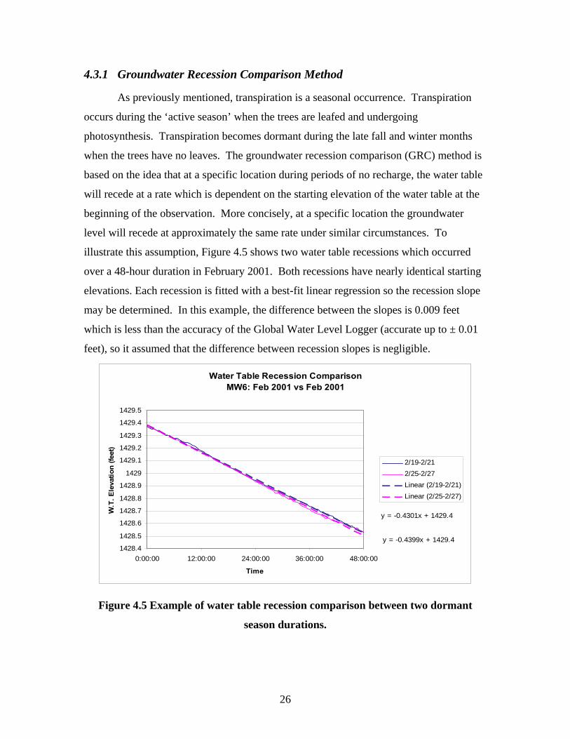
4.3.1 Groundwater Recession Comparison Method

As previously mentioned, transpiration is a seasonal occurrence. Transpiration

occurs during the ‘active season’ when the trees are leafed and undergoing

photosynthesis. Transpiration becomes dormant during the late fall and winter months

when the trees have no leaves. The groundwater recession comparison (GRC) method is

based on the idea that at a specific location during periods of no recharge, the water table

will recede at a rate which is dependent on the starting elevation of the water table at the

beginning of the observation. More concisely, at a specific location the groundwater

level will recede at approximately the same rate under similar circumstances. To

illustrate this assumption, Figure 4.5 shows two water table recessions which occurred

over a 48-hour duration in February 2001. Both recessions have nearly identical starting

elevations. Each recession is fitted with a best-fit linear regression so the recession slope

may be determined. In this example, the difference between the slopes is 0.009 feet

which is less than the accuracy of the Global Water Level Logger (accurate up to ± 0.01

feet), so it assumed that the difference between recession slopes is negligible.

Water Table Recession ComparisonMW6: Feb 2001 vs Feb 2001

y = -0.4301x + 1429.4

y = -0.4399x + 1429.41428.4

1428.5

1428.6

1428.7

1428.8

1428.9

1429

1429.1

1429.2

1429.3

1429.4

1429.5

0:00:00 12:00:00 24:00:00 36:00:00 48:00:00

Time

W.T

. Ele

vatio

n (fe

et)

2/19-2/212/25-2/27Linear (2/19-2/21)Linear (2/25-2/27)

Figure 4.5 Example of water table recession comparison between two dormant

season durations.

27

Rainfall is probably the most influential aspect of this analysis method. Recharge

resulting from rainfall events causes upward fluctuations in the water table making

recession comparisons nearly impossible. Since the GRC method is based on comparing

two recessions which start from the same elevation, it is difficult to find long durations

which are uninterrupted by rainfall. For this reason, most durations used in this study

were approximately 72 hours. Under ideal conditions however, the recession durations

would be longer.

With the observation that the water table recedes from similar starting elevations

at the same rate during time periods when the trees are inactive, it can be assumed that

the major difference between a recession rate measured during the active season and a

recession rate measured during dormant season (from similar starting elevations) is due to

evapotranspiration. If evaporation may be ruled out as a groundwater sink due to the

average depth (>2’) of the water table (White 1932, Freeze & Cherry 1979) and the

amount of vegetation and full canopy created by the hybrid poplars (Hillel 1998), the

primary difference between dormant and active season water table recessions can be

attributed to direct transpiration. An example of dormant recession (January) versus an

active recession (August) is shown in Figure 4.6. Note that each water table recession

starts at an elevation roughly equal to 1427.07 feet.

28

Water Table Recession ComparisonMW6: Jan 2002 vs August 2001

y = -0.1075x + 1427.1R2 = 0.9381

y = -0.1358x + 1427.1R2 = 0.9695

1426.60

1426.65

1426.70

1426.75

1426.80

1426.85

1426.90

1426.95

1427.00

1427.05

1427.10

0:00:00 12:00:00 24:00:00 36:00:00 48:00:00 60:00:00 72:00:00

Time

W.T

. Ele

vatio

n (fe

et)

1/15-1/188/19-8/22Linear (1/15-1/18)Linear (8/19-8/22)

Figure 4.6 Groundwater Recession Comparison: dormant versus active durations.

Transpiration, TDT (feet/day) is calculated by multiplying the difference between

the absolute values of the linear regression slopes and multiplying by specific yield,

SY = 0.1. The difference between the slopes in Figure 4.6 is 0.028; hence the direct

transpiration rate during the period between 8/19 and 8/22 is approximately 0.0028

feet/day.

4.3.2 White’s Equation

A second method for determining direct transpiration rates is White’s Equation

(White, 1932). This method focuses on diurnal water table fluctuations observed during

the active season to determine the rate of transpiration. During the day, it is expected that

the transpiring poplar trees surrounding the observation point create a groundwater sink

causing the elevation of water table to decrease. At night, the water table is expected to

recover in the absence of transpiration, so the water level in the piezometer temporarily

(until the sun rises) increases. White’s Equation uses this diurnal pattern to quantify

29

evapotranspiration. Figure 4.7 illustrates a period in August 2004 where diurnal

fluctuations were observed at the MW6 location.

Water Table Recession Analysis: White's EquationMW6: Augsust 2004

1425.90

1425.95

1426.00

1426.05

1426.10

1426.15

1426.20

1426.258/

13/0

4 0:

00

8/13

/04

12:0

0

8/14

/04

0:00

8/14

/04

12:0

0

8/15

/04

0:00

8/15

/04

12:0

0

8/16

/04

0:00

8/16

/04

12:0

0

8/17

/04

0:00

Date

W.T

. Ele

vatio

n (fe

et)

E = 0.05*Sy (24r+s)E = 0.05 (0.10+0.047)E = 0.0073 feet/day

24r = 0.10 feet

s = 0.047

Figure 4.7 Example of White’s Equation applied to August, 2004 MW6 data.

4.4 Determination of Direct Transpiration Flow Rates

Though useful, direct transpiration rates TDT (feet/day) are somewhat arbitrary

because they have no lateral boundaries. If it is assumed that the direct transpiration is

due to water consumption by the poplar trees, then it is logical to limit the extents of

these transpiration rates to the boundaries of the phytoremediation system. For this

reason, direct transpiration rates are multiplied by a representative land area in order to

calculate a volumetric direct transpiration rate, QDT (feet3/day). However, rather than

multiplying direct transpiration rates determined at each observation point by the total

area of the site, the rates were multiplied by smaller, equally-sized representative areas

surrounding each observation point. The primary reason for this was to account for

variability of direct transpiration rates due to spatial variability regarding differences in

the number of trees surrounding each point.

30

Based on the spacing of the tree rows, representative areas were created by

dividing the site into a grid containing 10 x 10 foot cells. The grid, shown in Figure 4.8,

was oriented with the direction of the tree rows and spatially located with regard to the

contaminant plume. The grid was sized large enough to contain the contaminant plume

and the trees which were available for contaminant uptake. The trees in the northwest

portion of the site were left out of the grid because there is no evidence of contamination

in that area.

Figure 4.8 Division of phytoremediation system into 10 x 10 foot cells.

To establish representative areas, a block of cells was assigned to each of the

points of observation: MW6, P4, and P25. Each block of cells contained the point of

observation within its center cell. A center cell plus the eight cells immediately adjacent

comprised a 900 square-foot area (3 cells x 3 cells) surrounding each observation point.

Next, the representative areas were increased to 5-cell x 5-cell blocks equal to 2500

square feet. This was the maximum area which could be used without overlapping

representative areas. Figures 4.9 and 4.10 illustrate both representative area sizes.

31

Figure 4.9 Representative 900 square-foot area around each observation point.

Figure 4.10 Representative 2500 square-foot area around each observation point.

32

If the volumetric rate of water leaving the representative areas can be attributed to

direct transpiration, then that rate can be divided by the number of trees within the

representative area to calculate the volumetric rate of direct transpiration in cubic feet per

day per tree. However, since it was known that the size of the trees within each area

varies and that the variability of transpiration rates between trees can be correlated to tree

diameter, the volumetric direct transpiration rate for the area was distributed amongst the

trees within that area based on tree diameter to yield per tree volumetric direct

transpiration rates, QTDT (gal/day-tree).

The first step to distributing volumetric transpiration rates to trees located within a

specific area was to determine the diameters of each tree found within that area. Calder

(1993) showed that tree transpiration is directly correlated to the square of diameter at

breast height (DBH). First the sum of the squares of the diameters within the area is

calculated. Then, the square of the DBH of each individual tree is divided by the sum of

the squares of all the tree diameters within the representative area to yield volumetric

transpiration for the individual tree. An example using a 900 square-foot area around

MW6 is shown:

dayfeetTDT 01.0= 2900 feetA =

dayfeetfeetx

dayfeetAxTQ DTDT

32

)900( 0.9)900()01.0()()( ===

⎟⎟⎟⎟

⎠

⎞

⎜⎜⎜⎜

⎝

⎛

=

∑N

i

iDTDT

Ti xQQ

1

)900( )(β

β

where: βi = (DBHi)2

DBHi = diameter at breast height of any tree, i

N = number of trees within representative area

This calculation is performed for every tree within the representative area and tabulated.

Table 4.3 illustrates this calculation and distribution.

33

Table 4.3 Sample calculation for estimating the volumetric transpiration rates of

trees within a nine-cell (900 ft2) area surrounding the observation point (MW6).

MW6-AVERAGE MONTHLY TRANSPIRATION VALUES DISTRIBUTED OVER SURROUNDING 900 SQ. FT AREA MAY 6, 2004 TRANSPIRATION RATE RECORDED AT MW6 = 0.00999 ft/day

QDTi = TDT x Acell = 0.00999 ft/day x 30' x 30' = 8.991 ft3/day βi = (DBHi)2

QTDTi = QDTi x ∑

N

i1

/ ββ

Cell # Tree Circum DBH β β/Σβ QTDTi QT

DTi i,j # (feet) (feet) (feet2) - (ft3/day-tree) (gal/day-tree)

3T4 1.21 0.39 0.1483 0.057 0.512 3.832 11,15 3T5 1.29 0.41 0.1686 0.065 0.582 4.356 3T1 1.21 0.39 0.1483 0.057 0.512 3.832 11,16 3T2 1.42 0.45 0.2043 0.078 0.706 5.278

11,17 11T1 1.58 0.50 0.2529 0.097 0.874 6.534 2T1 1.29 0.41 0.1686 0.065 0.582 4.356 2T2 0.94 0.30 0.0895 0.034 0.309 2.313 12,15

2T3 0.75 0.24 0.0570 0.022 0.197 1.472 1T12 1 0.32 0.1013 0.039 0.350 2.617 1T13 1 0.32 0.1013 0.039 0.350 2.617 1T14 1.42 0.45 0.2043 0.078 0.706 5.278

13,15

1T15 1.13 0.36 0.1294 0.050 0.447 3.342 1T8 0.75 0.24 0.0570 0.022 0.197 1.472 1T9 0.75 0.24 0.0570 0.022 0.197 1.472 13,16

1T10 1.42 0.45 0.2043 0.078 0.706 5.278 1T4 1.25 0.40 0.1583 0.061 0.547 4.090

1T5 0.67 0.21 0.0455 0.017 0.157 1.175

1T6 1.17 0.37 0.1387 0.053 0.479 3.583 13,17

1T7 1.29 0.41 0.1686 0.065 0.582 4.356

SUM 2.603 1.000 8.991 67.253 The first step of this calculation was to multiply the direct transpiration rate, TDT

(feet/day) recorded at MW6 on May 6, 2004 by the 900 square-foot representative area to

yield a volumetric transpiration rate (QDT) of 8.991 ft3/day. This value was then

distributed to the trees within the 900 square-foot area based a weighting factor which is

the square of the diameter at breast height (DBH). The volumetric direct transpiration

rate per tree is found for each tree within the representative area by multiplying QDT by

the fraction of the square of the tree diameter within the area (βi / ∑N

1βi). The result is a per

tree volumetric transpiration rate for each tree within that area. In the last step, units of

cubic feet per day-tree were converted to gallons per day-tree.

34

The calculation shown in Table 4.3 was made for each direct transpiration rate

determined by the Groundwater Recession Comparison method and by White’s Equation

for each observation point over both a 900 and 2500 square foot area. Plotting QTDT

versus DBH yields a power equation y = kx2 where k is the per tree volumetric direct

transpiration coefficient. An example is illustrated in Figure 4.11. Two k-values were

determined for each calculated transpiration (TDT ) rate: one for the 900 square-foot area

and one for the 2500 square foot area. These k-values were then used to form

relationships with other parameters such as time of year and saturated thickness.

Ultimately, k-values from each of the 3 observation locations (P4, P25, and MW6) were

applied to all of the trees on site so that a range of per tree volumetric direct transpiration

rates could be established for the entire phytoremediation system.

MW6: May 6, 2004, TDT=0.00999 ft/day, 900 sq ft Area

y = 25.833x2

0.0

1.0

2.0

3.0

4.0

5.0

6.0

7.0

0.00 0.10 0.20 0.30 0.40 0.50 0.60

DBH, Tree Diameter (feet)

QT D

T (ga

l/day

)

Figure 4.11 Range of per tree direct transpiration rates around MW6 for May 6,

2004 duration.

4.5 Determination of the Direct Uptake of Naphthalene

The final objective of this research is to determine the amount of naphthalene

mass leaving the system via direct uptake. This is accomplished by overlaying the

transpiration site grid with the naphthalene concentration data and then multiplying

35

volumetric transpiration rates by chemical concentration data and the Transpiration

Stream Coefficient Factor (TSCF) in each cell. The sum of all the cells yields a mass loss

rate of naphthalene in mg/day leaving the system.

4.5.1 Naphthalene Concentration Data

Chemical concentration data has been monitored at the Oneida phytoremediation

site since the project’s inception (Widdowson et al, 2005). Groundwater samples were

taken from the multilevel samplers which are located in the contaminant zone illustrated

in Figure 4.12. Concentrations were measured twice a year from the multilevel samplers

Figure 4.12 Location of multilevel samplers at the Oneida phytoremediation site.

and recorded in a spreadsheet. As previously mentioned, for every multilevel sampler,

there are up to eight ports from which to sample, each representing a different depth

within the subsurface (ranging from approximately 3 to 11 feet below land surface). As

observed by continuous water level records, the saturated thickness of the aquifer varies

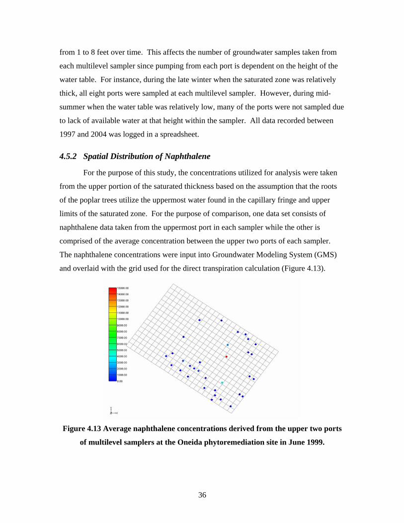
36

from 1 to 8 feet over time. This affects the number of groundwater samples taken from

each multilevel sampler since pumping from each port is dependent on the height of the

water table. For instance, during the late winter when the saturated zone was relatively

thick, all eight ports were sampled at each multilevel sampler. However, during mid-

summer when the water table was relatively low, many of the ports were not sampled due

to lack of available water at that height within the sampler. All data recorded between

1997 and 2004 was logged in a spreadsheet.

4.5.2 Spatial Distribution of Naphthalene

For the purpose of this study, the concentrations utilized for analysis were taken

from the upper portion of the saturated thickness based on the assumption that the roots

of the poplar trees utilize the uppermost water found in the capillary fringe and upper

limits of the saturated zone. For the purpose of comparison, one data set consists of

naphthalene data taken from the uppermost port in each sampler while the other is

comprised of the average concentration between the upper two ports of each sampler.

The naphthalene concentrations were input into Groundwater Modeling System (GMS)

and overlaid with the grid used for the direct transpiration calculation (Figure 4.13).

Figure 4.13 Average naphthalene concentrations derived from the upper two ports

of multilevel samplers at the Oneida phytoremediation site in June 1999.

37

Using a linear interpolation scheme within GMS, groundwater concentration contours

were generated for each of the naphthalene data sets. To better identity the lowest

naphthalene concentration, additional points were added around the periphery of the

plume boundary. The output from GMS provides the interpolated naphthalene

concentration for each cell. An example of this interpolation scheme is illustrated in

Figure 4.14.

Figure 4.14 Oneida phytoremediation system naphthalene concentration contours

interpolated from point measurements taken in June 1999.

4.5.3 Calculation of Mass Removal of Naphthalene via Plant Uptake

Using the concentration of naphthalene of each cell, the equation to calculate plant uptake

is: Ucell = (TSCF) (Tcell) (Ccell) (5.1)

where: Ucell = rate of contaminant uptake in a given cell (mg/day),

TSCF = Transpiration Stream Concentration Factor (unitless),

Tcell = sum of volumetric direct transpiration of trees within cell (L/day),

Ccell = soil water concentration of naphthalene (mg/L).

The TSCF is calculated using the following equation developed by Burken and Schnoor

(1998):

38

( )304.0

44.278.1log

784.02

)( =⎟⎟

⎠

⎞

⎜⎜

⎝

⎛ −−×= NapthaleneKow

EXPTSCF

The overall rate of removal for the site is the sum of all Ucell values. The value for Tcell is

the direct transpiration rates estimated for the particular day concentration data was

measured.

4.5.4 Plot of Discrete Water Level Measurements

Discrete water level measurements performed on a monthly basis were used to

create groundwater contours and water table profiles. To-scale mapping of the water

table at the Oneida site is useful for observing water table elevation trends across this site.

4.5.5 Groundwater Contours

Groundwater contours were created by digitizing recorded water table elevations

using AutoCAD Land Development™ software which linearly interpolated between

point elevations (discrete water level measurements). These contours were used to

establish hydraulic gradient and direction of flow. In addition, by analyzing the

groundwater contours over time (on a monthly basis), the existence of cone of depression

created by the transpiring trees could be determined. An example of groundwater

contours for the Oneida phytoremediation site for March 6, 2004 is illustrated in Figure

4.15.

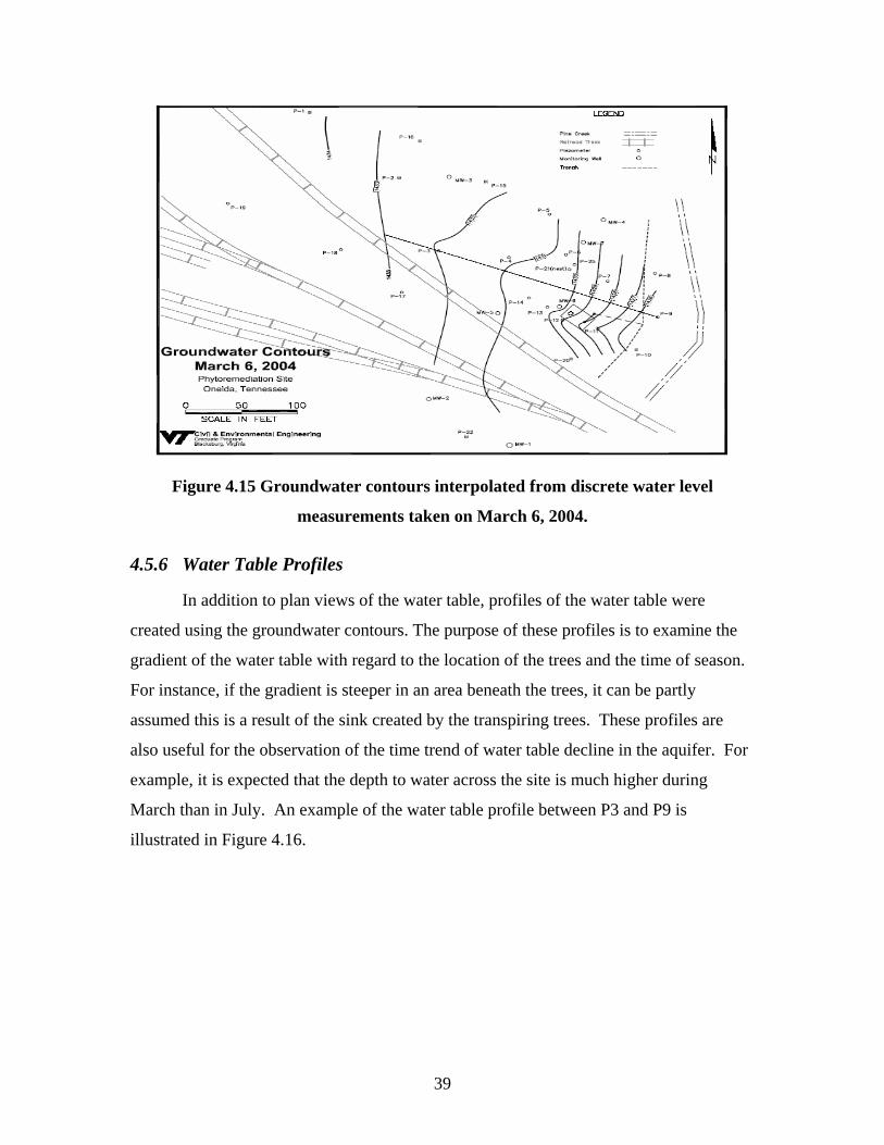
39

Figure 4.15 Groundwater contours interpolated from discrete water level

measurements taken on March 6, 2004.

4.5.6 Water Table Profiles

In addition to plan views of the water table, profiles of the water table were

created using the groundwater contours. The purpose of these profiles is to examine the

gradient of the water table with regard to the location of the trees and the time of season.

For instance, if the gradient is steeper in an area beneath the trees, it can be partly

assumed this is a result of the sink created by the transpiring trees. These profiles are

also useful for the observation of the time trend of water table decline in the aquifer. For

example, it is expected that the depth to water across the site is much higher during

March than in July. An example of the water table profile between P3 and P9 is

illustrated in Figure 4.16.

40

Figure 4.16 Water table profile and groundwater contours for March 6, 2004. The

profile line with station labels 0+00 to 2+63 intersects P3 and P9.

Ultimately, the plan and profile of a series of groundwater contours collected

between March and October was used to develop conclusions about the impact of the

phytoremediation system on the saturated thickness of the shallow aquifer underlying the

Oneida site.

41

5 RESULTS AND DISCUSSION

5.1 Summary of Data Utilized for this Study

During the course of this analysis, a variety of data sources were used to complete

the objectives of this project. To gain understanding about transpiration rates and plant

uptake of naphthalene at the Oneida phytoremediation site, continuous water level data

collected in 2004 were analyzed and compared with data previously collected by others

between 1998 and 2003. Weather data were recorded from March through October 2004

using an on-site weather station. Additional rainfall data were compiled from records by

the National Climatic Data Center (NCDC). Intermittent on-site weather data recorded

between 2000 and 2003 were collected by others. Between 1997 and 2004, naphthalene

concentration data from groundwater were collected bi-annually from multilevel

samplers. Discrete water level measurements were performed on a monthly basis for this

study between March 2004 and October 2004. Discrete water level measurements taken

by others were available for 1998 through 2001.

5.1.1 Oneida Rainfall Data

Rainfall amounts were collected intermittently on-site between 2000 and 2004. In

order to have continuous monthly and yearly rainfall amounts at Oneida, site weather

station data were subsidized with local rainfall data collected at the Oneida wastewater

treatment plant (WWTP). Besides the on-site weather station, the wastewater treatment

plant rain gauge is the closest recorded rain gauge to the phytoremediation site. All rain

data logged at the Oneida WWTP are recorded into the National Climatic Data Center

database and are available for public use online at:

http://www.ncdc.noaa.gov/oa/ncdc.html.

To make assumptions about the impacts of rainfall on groundwater levels at the

Oneida site, yearly rainfall records were compared to long-time averages. This was

important because drought years can have significant impacts on tree performance and

wet years can potentially influence the mobility of the contaminant plume. A summary

of monthly rainfall from 1999-2004 is shown in Table 5.1 and a comparison of yearly

totals (1999-2004) versus 100-year average yearly totals is illustrated in Figure 5.1.

42

Table 5.1 Precipitation record for Oneida, Tennessee. Rain gauge located at Oneida

wastewater treatment plant (WWTP). Data Source: National Climatic Data Center.

Precipitation Record for Oneida, Tennessee 2004 2003 2002 2001 2000 1999 100-Year

Observed Month

(inches) (inches) (inches) (inches) (inches) (inches) Average*J 1.82 1.83 7.26 4.09 4.14 8.03 4.7 F 4.28 9.37 2.31 5.88 4.19 4.37 4.2 M 2.82 1.46 10.23 3.94 3.24 3.85 5.5 A 4.28 9.58 3.06 2.49 6.32 4.38 4.2 M 5.89 6.28 4.68 3.46 4.54 4.29 5.5 J 3.00 8.70 4.64 3.88 6.21 7.13 4.8 J 5.00 4.19 3.47 5.99 2.39 4.53 5.0 A 5.50 4.72 2.39 2.47 2.45 2.67 4.5 S 7.52 8.89 5.73 3.77 1.74 0.6 3.7 O 3.78 2.27 3.18 3.07 0.57 2.47 3.7 N 5.74 4.77 4.10 2.88 2.53 2.62 4.5 D 4.80 3.62 6.82 4.53 2.75 2.31 4.8

Year Total 54.43 65.68 57.87 46.45 41.07 47.25 55.1

Monthly Rainfall Totals for Oneida, TN Rain Gauge Location: Oneida WWTP

0.00

2.00

4.00

6.00

8.00

10.00

12.00

J F M A M J J A S O N D

Month

Rai

nafa

ll (in

ches

) 200420032002200120001999Average

Figure 5.1 Comparison of monthly rainfall totals from 1999 to 2004 and 100-year

average.

43

Rainfall, the source of recharge, is a significant parameter with regard to

groundwater levels and direct transpiration. Due to its consistency, rainfall data recorded

from 1999-2004 at the Oneida WWTP were used to determine yearly and monthly trends.

In general, yearly rainfall values were used to determine if a particular year was above or

below average. Table 5.1 shows that during 2004, Oneida received an average amount of

rainfall, 2003 was a relatively ‘wet’ year, 2002 was about average, and 2001, 2000, and

1999 were probably considered drought years. For a phytoremediation system, however,

it is equally important to observe monthly rainfall trends. Monthly rainfall averages are

important since a phytoremediation system only impacts groundwater levels between

March and October. For instance, though 2004 as a whole appeared average, June was

relatively dry compared to the average (3.0 versus 4.8 inches). September 2004 was

significantly above average with 7.58 inches versus the average 3.70 inches. Though not

considered a drought year by yearly averages, 2002 received below average rainfall from

April through October; months when the phytoremediation system was considered to be

active.

During 2004, the weather station at the Oneida phytoremediation site operated

continuously from March 6th to October 8th and recorded on a half-hour interval. This

relatively short interval indicated precise occurrences of rainfall on-site. For the purpose

of determining direct transpiration rates, it was important to know exactly when rainfall

occurred at the Oneida phytoremediation site because the Groundwater Recession

Comparison method and White’s Equation must be performed during periods which were

not immediately influenced by rainfall. Figure 5.3 illustrates the rainfall record from the

weather station for 2004.

44

Figure 5.2 Rainfall recorded by weather station at phytoremediation site, 2004.

The values reported from the phytoremediation site weather station during August

2004 were skewed by a weather station malfunction which occurred between August 20th

and September 3rd. During that time, the Oneida WWTP indicated that it rained a total of

2.26 inches.

5.1.2 Continuously Recorded Water Table Elevations

The type of groundwater data primarily used for the quantification of direct

transpiration rates were water level data which were continuously recorded from

observation points MW6, P4, and P25. For the 2004 season, three Global Level Loggers

were utilized to collect water level data from piezometers MW6, P4, and P25. These

observation points were chosen for two reasons: 1) All were close to or within the

contaminant plume area and 2) previous data existed from these locations which were

used for comparison. The transducers were set on March 6, 2004. In April 2004 a

fourth Global Level Logger was placed in P3. A summary of water level data (with

rainfall data) from MW6, P4, P25, and P3 is illustrated in Figures 5.3-5.4.

45

W.T. Elevation & Rainfall 2004

1423

1425

1427

1429

1431

1433

J F M A M J J A S O N D

Date

W.T

. Ele

vatio

n (fe

et)

0

1

2

3

4

5

6

7

8

9

10

Rai

nfal

l (in

ches

)

P4

MW6

P3

P25

Rain

Figure 5.3 Continuous water table elevation and rainfall data from 2004.

W.T. Elevation & Rainfall 2003

1423

1425

1427

1429

1431

1433

J F M A M J J A S O N D

Date

W.T

. Ele

vatio

n (fe

et)

0

1

2

3

4

5

6

7

8

9

10

Rai

nfal

l (in

ches

)

MW6

P25

Rain

W.T. Elevation & Rainfall 2002

1423

1425

1427

1429

1431

1433

J F M A M J J A S O N D

Date

W.T

. Ele

vatio

n (fe

et)

0

1

2

3

4

5

6

7

8

9

10

Rai

nfal

l (in

ches

)

MW6

Rain

W.T. Elevation & Rainfall

2001

1423

1425

1427

1429

1431

1433

J F M A M J J A S O N D

Date

W.T

. Ele

vatio

n (fe

et)

0

1

2

3

4

5

6

7

8

9

10

Rai

nfal

l (in

ches

)

MW6

P4

Rain

W.T. Elevation & Rainfall 2000

1423

1425

1427

1429

1431

1433

J F M A M J J A S O N D

Date

W.T

. Ele

vatio

n (fe

et)

0

1

2

3

4

5

6

7

8

9

10

Rai

nfal

l (in

ches

)

P4

MW6

Rain

Figure 5.4Continuous water table elevation and rainfall data, 2000-2003.

46

It is evident from Figures 5.3 – 5.4 that precipitation influences water levels at the Oneida

phytoremediation site. During times of significant rainfall (long durations of light

rainfall, short durations of intense rainfall, or both), the elevation of the water table at the

three observation points increased, sometimes dramatically. The magnitude of

fluctuations tends to change over the course of one year depending on the season. During

the first part of the year (winter and early spring), precipitation caused the water levels in

the piezometers to increase dramatically. Depending on the nature of the rain event, this

tendency was subject to variance. During the late spring through mid to late summer,

rainfall of similar quantities tended to cause fluctuations of the water table of a magnitude

which was smaller than that seen during the first part of the year. A return to greater

fluctuations occurred at the beginning of the fall season and continues through winter.

This trend can be observed during 2004, 2002, 2001, and 2000. This trend is observed to

a lesser degree during 2003 due to large amounts of consistent rainfall which fell during

that year. In addition, P3 data illustrated in Figure 5.3 exhibited greater fluctuations in

water levels resulting from rain events during the late spring and summer than MW6, P4,

and P25. It should be noted that P3 is not found within the dense area of trees, but rather

in an open area with less than 10 poplar trees within a 50-foot radius. This suggests that

transpiring trees influence the recession of the water table.

The relationship between rainfall and water levels was most apparent at MW6 due

to consistent data which were collected there between 2001 and 2004. With regard to

rainfall, 2004 was relatively average while 2001 was considered a drought year. This

difference is evident when comparing water table elevations observed at MW6 during

2004 and 2001 (Figures 5.5). For simplicity, a 15-day running average for MW6 data was

employed in order to better illustrate groundwater trends. As a result of average rainfall

during summer 2004, the water table elevation at MW6 remained consistently near1426

feet. As a result of below average rainfall during summer 2001, the water table elevation

at MW6 remained below 1426 feet for a relatively long duration. The elevation dipped

below 1425 feet in July 2001.

47

MW6 W.T. Elevation and Rainfall

1424

1425

1426

1427

1428

1429

1430

M A M J J A S O

Month (2004)

W.T

. Ele

vatio

n (fe

et)

0.0

0.3

0.7

1.0

1.3

1.7

2.0

Rai

nfal

l (in

ches

)

MW6-W.T. Elev Rainfall

MW6 W.T. Elevation and Rainfall

1424

1425

1426

1427

1428

1429

1430

J F M A M J J A S

Date (2001)

W.T

. Ele

vatio

n (fe

et)

0.0

0.3

0.7

1.0

1.3

1.7

2.0

Rai

nfal

l (in

ches

)

MW6 W.T. Elev Rainfall Figure 5.5 Running average of continuous water table elevation and daily rainfall

data from 2004 and 2001.

5.1.3 Discrete Water Level Data

The overall trend of groundwater levels indicated a noticeable decrease between

spring and summer. Measurements were performed once a month through October and

are shown in Table 5.2. The first round of discrete water level measurements occurred on

March 6, 2004.

Water levels decreased relatively significantly between March 6, 2004 and April 24,

2004. During the period, the trees on-site became leafed and began the seasonal

transpiration process. From April 24th through October 8th while the trees were leafed,

groundwater levels at the Oneida phytoremediation remained relatively low. With

respect to the recording location, no water level recorded between April and October

(active season) exceeded the water levels recorded during March (dormant season). In

addition, water table elevations in some piezometers were not detected because the

elevation of the water table was below the bottom of casing of the piezometer (indicated

by “dry” in Table 5.2). This was evident in P4, P8, P20, P21A, P21B, and P21C in

August and early September.

Rainfall amounts recorded between March and October 2004 (Table 5.1 and

Figure 5.2) indicate that March received the least rainfall of all the months during which

discrete water level measurements were performed in 2004. This indicates between

March 6th and April 24th an additional sink for groundwater was created by the hybrid

poplars and continued into early October.

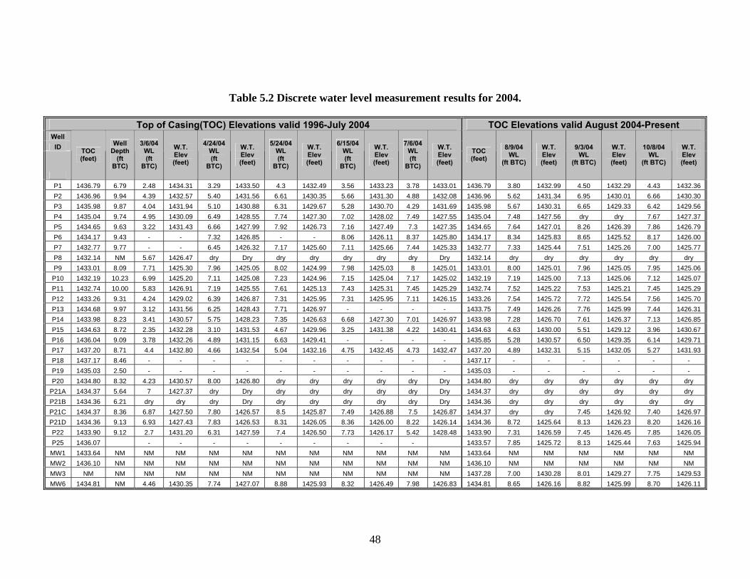
48

Table 5.2 Discrete water level measurement results for 2004.

Top of Casing(TOC) Elevations valid 1996-July 2004 TOC Elevations valid August 2004-Present Well ID

TOC (feet)

Well Depth

(ft BTC)

3/6/04 WL (ft

BTC)

W.T. Elev (feet)

4/24/04 WL (ft

BTC)

W.T. Elev (feet)

5/24/04 WL (ft

BTC)

W.T. Elev (feet)

6/15/04 WL (ft

BTC)

W.T. Elev (feet)

7/6/04 WL (ft

BTC)

W.T. Elev (feet)

TOC (feet)

8/9/04 WL

(ft BTC)

W.T. Elev (feet)

9/3/04 WL

(ft BTC)

W.T. Elev (feet)

10/8/04 WL

(ft BTC)

W.T. Elev (feet)

P1 1436.79 6.79 2.48 1434.31 3.29 1433.50 4.3 1432.49 3.56 1433.23 3.78 1433.01 1436.79 3.80 1432.99 4.50 1432.29 4.43 1432.36 P2 1436.96 9.94 4.39 1432.57 5.40 1431.56 6.61 1430.35 5.66 1431.30 4.88 1432.08 1436.96 5.62 1431.34 6.95 1430.01 6.66 1430.30 P3 1435.98 9.87 4.04 1431.94 5.10 1430.88 6.31 1429.67 5.28 1430.70 4.29 1431.69 1435.98 5.67 1430.31 6.65 1429.33 6.42 1429.56 P4 1435.04 9.74 4.95 1430.09 6.49 1428.55 7.74 1427.30 7.02 1428.02 7.49 1427.55 1435.04 7.48 1427.56 dry dry 7.67 1427.37 P5 1434.65 9.63 3.22 1431.43 6.66 1427.99 7.92 1426.73 7.16 1427.49 7.3 1427.35 1434.65 7.64 1427.01 8.26 1426.39 7.86 1426.79 P6 1434.17 9.43 - - 7.32 1426.85 - - 8.06 1426.11 8.37 1425.80 1434.17 8.34 1425.83 8.65 1425.52 8.17 1426.00 P7 1432.77 9.77 - - 6.45 1426.32 7.17 1425.60 7.11 1425.66 7.44 1425.33 1432.77 7.33 1425.44 7.51 1425.26 7.00 1425.77 P8 1432.14 NM 5.67 1426.47 dry Dry dry dry dry dry dry Dry 1432.14 dry dry dry dry dry dry P9 1433.01 8.09 7.71 1425.30 7.96 1425.05 8.02 1424.99 7.98 1425.03 8 1425.01 1433.01 8.00 1425.01 7.96 1425.05 7.95 1425.06

P10 1432.19 10.23 6.99 1425.20 7.11 1425.08 7.23 1424.96 7.15 1425.04 7.17 1425.02 1432.19 7.19 1425.00 7.13 1425.06 7.12 1425.07 P11 1432.74 10.00 5.83 1426.91 7.19 1425.55 7.61 1425.13 7.43 1425.31 7.45 1425.29 1432.74 7.52 1425.22 7.53 1425.21 7.45 1425.29 P12 1433.26 9.31 4.24 1429.02 6.39 1426.87 7.31 1425.95 7.31 1425.95 7.11 1426.15 1433.26 7.54 1425.72 7.72 1425.54 7.56 1425.70 P13 1434.68 9.97 3.12 1431.56 6.25 1428.43 7.71 1426.97 - - - - 1433.75 7.49 1426.26 7.76 1425.99 7.44 1426.31 P14 1433.98 8.23 3.41 1430.57 5.75 1428.23 7.35 1426.63 6.68 1427.30 7.01 1426.97 1433.98 7.28 1426.70 7.61 1426.37 7.13 1426.85 P15 1434.63 8.72 2.35 1432.28 3.10 1431.53 4.67 1429.96 3.25 1431.38 4.22 1430.41 1434.63 4.63 1430.00 5.51 1429.12 3.96 1430.67 P16 1436.04 9.09 3.78 1432.26 4.89 1431.15 6.63 1429.41 - - - - 1435.85 5.28 1430.57 6.50 1429.35 6.14 1429.71 P17 1437.20 8.71 4.4 1432.80 4.66 1432.54 5.04 1432.16 4.75 1432.45 4.73 1432.47 1437.20 4.89 1432.31 5.15 1432.05 5.27 1431.93 P18 1437.17 8.46 - - - - - - - - - - 1437.17 - - - - - - P19 1435.03 2.50 - - - - - - - - - - 1435.03 - - - - - - P20 1434.80 8.32 4.23 1430.57 8.00 1426.80 dry dry dry dry dry Dry 1434.80 dry dry dry dry dry dry

P21A 1434.37 5.64 7 1427.37 dry Dry dry dry dry dry dry Dry 1434.37 dry dry dry dry dry dry P21B 1434.36 6.21 dry dry dry Dry dry dry dry dry dry Dry 1434.36 dry dry dry dry dry dry P21C 1434.37 8.36 6.87 1427.50 7.80 1426.57 8.5 1425.87 7.49 1426.88 7.5 1426.87 1434.37 dry dry 7.45 1426.92 7.40 1426.97 P21D 1434.36 9.13 6.93 1427.43 7.83 1426.53 8.31 1426.05 8.36 1426.00 8.22 1426.14 1434.36 8.72 1425.64 8.13 1426.23 8.20 1426.16 P22 1433.90 9.12 2.7 1431.20 6.31 1427.59 7.4 1426.50 7.73 1426.17 5.42 1428.48 1433.90 7.31 1426.59 7.45 1426.45 7.85 1426.05 P25 1436.07 - - - - - - - - - 1433.57 7.85 1425.72 8.13 1425.44 7.63 1425.94 MW1 1433.64 NM NM NM NM NM NM NM NM NM NM NM 1433.64 NM NM NM NM NM NM MW2 1436.10 NM NM NM NM NM NM NM NM NM NM NM 1436.10 NM NM NM NM NM NM MW3 NM NM NM NM NM NM NM NM NM NM NM NM 1437.28 7.00 1430.28 8.01 1429.27 7.75 1429.53 MW6 1434.81 NM 4.46 1430.35 7.74 1427.07 8.88 1425.93 8.32 1426.49 7.98 1426.83 1434.81 8.65 1426.16 8.82 1425.99 8.70 1426.11

49

5.1.4 Tree Growth

As of the last count in June 2004, the Oneida phytoremediation system had 693

live hybrid poplar trees whose diameters ranged from 0.5 to 7.5 inches. Based on tree

circumference, surviving trees grew approximately 16% between June 1998 and June

1999, 46 % between June 1999 and January 2001, and approximately 44% between June

2001 and June 2004. Between June 1998 and June 2004, the amount of live trees on-site

diminished from 1,036 to 693. Figure 5.6 illustrates overall tree growth and the decrease

in the number of trees between 1998 and 2004.

0

100

200

300

400

500

600

700

800

900

1000

1100

June 98 June 99 January 01 June 04

Num

ber o

f Liv

e Tr

ees

0

0.2

0.4

0.6

0.8

1

Ave

rage

Tre

e C

ircum

fere

nce

(feet

)

No. of Trees Avg Tree Circumference

Figure 5.6 Hybrid poplar growth and survival at Oneida site between 1999 and

2004.

With respect to tree diameter, the distribution of hybrid poplar trees on-site is

illustrated by Figure 5.7. Approximately 38% of the trees are between 0.20 and 0.29 feet

followed by 31.3 % between 0.10 and 0.19 feet. 6.35 % of the trees are between 0.40 and

0.49 feet in diameter and 3% of the trees on-site are below 0.10 feet in diameter. 1.87%

of the trees on-site are between 0.5 and 0.64 feet in diameter.

50

The average diameter within the 9-year old hybrid poplar stand at Oneida in June

2004 was 0.25 feet. At a 13-year old hybrid poplar stand in Flanders, Belgium, the

average diameter was 1.37 feet (Meiresonne et al, 1999). Though there is an age

difference, even if the size of the trees at Oneida increased 50% each year, the average

diameter would still be less than observed in Belgium. This relatively significant

difference indicates the trees at Oneida have not grown to their potential. The most

apparent indicator of this is the existence of trees on-site which are greater than 0.6 feet

in diameter. If some trees at the Oneida site were capable of growing to this size, then it

is logical that all of the trees could have grown to this size under the right circumstances.

The most noticeable difference between the two poplar stands (Oneida, TN and Flanders,

Belgium) is tree spacing. At Oneida, the trees are spaced 3 feet apart within rows which

are 10 feet apart. In Belgium, the trees were spaced 21 feet apart within rows which were

approximately 25 feet apart (Meiresonne et al, 1999). If variability of transpiration rates

between trees can be correlated to tree diameter, then tree spacing is a crucial component

to maximizing the volume of water directly transpired from the saturated zone (Vose et

al, 2003).

0

50

100

150

200

250

300

0.00-0.09 0.10-0.19 0.20-0.29 0.30-0.39 0.40-0.49 0.50-0.59 0.60-0.69

DBH, Tree Diameter (feet)

Num

ber o

f Tre

es (2

004)

Figure 5.7 Range of tree diameters found at Oneida site (Total = 693), June 2004.

51

5.2 Quantification of Direct Transpiration Rates

5.2.1 Results of Groundwater Recession Comparison Method

To quantify direct transpiration TDT (feet/day) using the Groundwater Recession

Comparison (GRC) method, two groundwater recessions of similar time lengths and

starting elevations from the same observation point are necessary. One groundwater

recession duration must be from the dormant season when the trees are not active and the

other from the active season when the trees are leafed. For the purpose of this study,

active durations were chosen from the 2004 season only while dormant durations were

chosen from both 2004 and previous years. The dormant season was considered to be

from mid-October to mid-March and the active season from mid-to-late March to mid-

October. This is approximately equivalent to the average 150-day growing season for the

Oneida area. This determination of the dormant and active seasons was substantiated by

observations of leaf quantity on trees at the Oneida site. The trees first began to be

foliated at the end of March, were significantly leafed by mid-April, and were completely

leafed by mid-May. Leaves began to fall very early (early July) but the trees still had

significant leaf coverage through August. By early September, approximately 50% of the

leaves had fallen and by October 8th nearly all of the leaves had fallen.

Examples of the Groundwater Recession Comparison method for MW6 are

shown in Figure 5.8. This sequence was used to calculate direct transpiration rates from

nearly the beginning of the active season until nearly the end. The durations used for the

GRC method were limited to 72 hours since rainfall usually occurred within one to two

days of the time of observation. All groundwater recessions were fitted with a ‘best-fit’

linear regression so that slopes could be determined. It was desired that R2 values for the

linear regression remain above 0.9, though this was not the case for both July and

October. During periods when the water table elevations were relatively and consistently

low, data recorded by the transducer at MW6 exhibited irregular fluctuations referred to

as “noise”. This can be observed in Figures 5.3-5.4 when the water table elevation gets

below 1426 feet. This problem was attributed to an aging sensor which was eventually

replaced in August 2004. For the July regression data set, a 10-value running average

was implemented to cut down on “noise” and achieve a linear regression. No other direct

52

transpiration rates could be determined during for July due to a lack of data which could

be used for comparison. In July 2004, the elevation of the water table falls below 1426

feet. Besides January 2001, no other dormant water table elevation data between 1426

and 1425.5 feet existed which was not interrupted by a rain event. In addition, a

malfunction occurred on July 19, 2004 which caused the level logger to stop recording

data. No water level data was recorded at MW6 between July 19th and August 9th during

2004.

Water Table Recession ComparisonMW6: March 2004 vs April 2004

y = -0.1515x + 1427.9R2 = 0.9928

y = -0.1946x + 1427.9R2 = 0.99321427.30

1427.40

1427.50

1427.60

1427.70

1427.80

1427.90

1428.00

0:00:00 12:00:00 24:00:00 36:00:00 48:00:00 60:00:00 72:00:00

Duration (hours)

W.T

. Ele

vatio

n (fe

et)

3/12-3/154/18-4/21Linear (3/12-3/15)Linear (4/18-4/21)

Water Table Recession ComparisonMW6: January 2002 vs May 2004

y = -0.0963x + 1427R2 = 0.9551

y = -0.1962x + 1427R2 = 0.9768

1426.40

1426.50

1426.60

1426.70

1426.80

1426.90

1427.00

1427.10

0:00:00 12:00:00 24:00:00 36:00:00 48:00:00 60:00:00 72:00:00

Duration (hours)

W.T

. Ele

vatio

n (fe

et)

1/15-1/175/6-5/8Lin 1/15-1/17Lin 5/6-5/8

Water Table Recession Comparison MW6: Feb 2002 vs June 2004

y = -0.0868x + 1427.4R2 = 0.9363

y = -0.1332x + 1427.4R2 = 0.9626

1426.9

1426.95

1427

1427.05

1427.1

1427.15

1427.2

1427.25

1427.3

1427.35

1427.4

0:00:00 12:00:00 24:00:00 36:00:00 48:00:00 60:00:00 72:00:00

Duration (hours)

W.T

. Ele

vatio

n (fe

et)

2/23-2/266/5-6/8Linear (2/23-2/26)Linear (6/5-6/8)

Water Table Recession Comparison MW6: January 2001 vs July 2004

y = -0.0227x + 1426.2R2 = 0.7404

y = -0.0552x + 1426.2R2 = 0.6566

1426

1426.05

1426.1

1426.15

1426.2

1426.25

1426.3

1426.35

0:00:00 12:00:00 24:00:00 36:00:00 48:00:00 60:00:00 72:00:00

Duration (hours)

W.T

. Ele

vatio

n (fe

et)

01/14-01/1707/09-07/12Linear (01/14-01/17)Linear (07/09-07/12)

Water Table Recession ComparisonMW6: Feb 02 vs Sept 04

y = -0.0868x + 1427.4R2 = 0.9363

y = -0.1508x + 1427.4R2 = 0.968

1426.8

1426.9

1427

1427.1

1427.2

1427.3

1427.4

1427.5

0:00:00 12:00:00 24:00:00 36:00:00 48:00:00 60:00:00 72:00:00

Duration (hours)

W.T

. Ele

vatio

n (fe

et)

2/23-2/269/10-9/13Linear (2/23-2/26)Linear (9/10-9/13)

Water Table Recession ComparisonMW6: Jan 2001 vs Oct 2004

y = -0.0241x + 1426.2R2 = 0.7965

y = -0.0379x + 1426.2R2 = 0.8601

1426.05

1426.1

1426.15

1426.2

1426.25

1426.3

0:00:00 12:00:00 24:00:00 36:00:00 48:00:00 60:00:00 72:00:00

Duration (hours)

W.T

. Ele

vatio

n (fe

et)

1/14-1/1710/3-10/6Linear (1/14-1/17)Linear (10/3-10/6)

Figure 5.8 Groundwater Recession Comparison method series for MW6.

53

The Groundwater Recession Comparison method yielded twenty direct

transpiration rates for the active season (Table 5.3). Direct transpiration values calculated

via the GRC method ranged from 0.0028 to 0.0100 feet/day during the active season. For

the purpose of comparison, three values were determined for the dormant season.

Ideally, dormant season direct transpiration rates would be 0.00 feet/day since

transpiration does not occur during this time when the trees have no leaves. The values

calculated for dormant dates ranged from 0.0001 to 0.001 feet/day. This indicates that

from a specific elevation, the water table does not recede at an absolutely consistent rate.

However, it should be re-stated that the accuracy of the level logger is ±0.01 feet and that

a slope difference of ±0.01 feet would result in the calculation of a direct transpiration

rate of 0.001 feet/day. Thus, direct transpiration rates are only accurate to the nearest

0.001 feet/day.

Table 5.3 Direct transpiration rates, TDT (feet/day) calculated for 2004 from

observation points MW6, P4, and P25.

GW Recession A GW Recession B TDT Well Dormant Avg Slope Active Avg Slope Sy=0.10

#

Starting W.T. Elev (feet)

Year Date (ft/d)

Year Date (ft/d)

Difference (absolute)

(feet/day) MW6 1429.38 2001 19-Feb -0.4301 2001 21-Feb -0.4399 0.0098 0.0010 MW6 1427.91 2004 12-Mar -0.1431 2004 23-Mar -0.1477 0.0046 0.0005 MW6 1427.93 2004 12-Mar -0.1515 2004 18-Apr -0.1946 0.0431 0.0043 MW6 1427.03 2002 15-Jan -0.0963 2004 6-May -0.1962 0.0999 0.0100 MW6 1427.36 2002 23-Feb -0.0868 2004 5-Jun -0.1332 0.0464 0.0046 MW6 1426.23 2001 14-Jan -0.0227 2004 9-Jul -0.0552 0.0325 0.0033 MW6 1427.05 2002 15-Jan -0.1075 2001 19-Aug -0.1358 0.0283 0.0028 MW6 1427.36 2002 23-Feb -0.0868 2004 10-Sep -0.1508 0.0640 0.0064 MW6 1427.05 2002 15-Jan -0.1075 2004 23-Sep -0.1408 0.0333 0.0033 MW6 1426.23 2001 14-Jan -0.0241 2004 3-Oct -0.0379 0.0138 0.0014 MW6 1427.50 2001 6-Jan -0.2065 2003 24-Dec -0.2056 0.0009 0.0001

P4 1428.69 2004 13-Mar -0.0508 2004 4-Apr -0.0817 0.0309 0.0031 P4 1428.69 2004 13-Mar -0.0508 2004 27-Apr -0.0927 0.0419 0.0042 P4 1428.50 2004 26-Mar -0.0640 2004 5-May -0.1308 0.0668 0.0067 P4 1428.50 2004 26-Mar -0.0617 2004 7-Jun -0.0949 0.0332 0.0033 P4 1429.85 2001 22-Jan -0.3039 2004 18-Sep -0.3488 0.0449 0.0045 P4 1428.70 2004 24-Mar -0.0720 2004 22-Sep -0.1051 0.0331 0.0033 P4 1428.50 2004 24-Mar -0.0640 2004 23-Sep -0.1030 0.0390 0.0039

P25 1427.50 2004 8-Feb -0.2013 2004 7-Mar -0.2074 0.0061 0.0006 P25 1426.75 2004 13-Feb -0.0612 2004 2-Apr -0.0899 0.0287 0.0029 P25 1426.50 2004 16-Mar -0.0255 2004 21-Apr -0.1052 0.0797 0.0080 P25 1427.23 2004 10-Feb -0.1335 2004 19-Sep -0.1682 0.0347 0.0035 P25 1426.50 2004 16-Mar -0.0255 2004 23-Sep -0.0538 0.0283 0.0028

54

5.2.2 Results of White’s Equation

The results of the application of White’s equation to 2004 continuous water level

records yielded only two values for direct transpiration. The primary reason is due to the

lack of diurnal patterns observed during the active season. It is not known why diurnal

patterns were so scarce at the Oneida site, but aquifer heterogeneity and depth to water

may be influential factors. The Oneida site aquifer contains stratified layers of course

and fine grained material. These different materials, found at different elevations within

the aquifer, probably yield groundwater at different rates. For instance, if diurnal

fluctuations were observed at a specific piezometer at an elevation where a course

grained material was found, then diurnal fluctuations might not be observed at the same

piezometer when the water table was within a layer of fine grained material. Figure 5.9

illustrate the results of applying White’s Equation to Oneida water table data and Table

5.4 tabulates the results.

Water Table Recession Analysis: White's EquationP25: May 2004

1425.75

1425.80

1425.85

1425.90

1425.95

1426.00

1426.05

1426.10

1426.15

1426.20

1426.25

5/3/

04 0

:00

5/3/

04 1

2:00

5/4/

04 0

:00

5/4/

04 1

2:00

5/5/

04 0

:00

5/5/

04 1

2:00

5/6/

04 0

:00

5/6/

04 1

2:00

5/7/

04 0

:00

Date

W.T

. Ele

vatio

n (fe

et)

E = 0.05*Sy (24r+s)E = 0.05 (0.10+0.0625)E = 0.0081 feet/day

24r = 0.10 feet

s = 0.0625 feet

Water Table Recession Analysis: White's EquationMW6: Augsust 2004

1425.90

1425.95

1426.00

1426.05

1426.10

1426.15

1426.20

1426.25

8/13

/04

0:00

8/13

/04

12:0

0

8/14

/04

0:00

8/14

/04

12:0

0

8/15

/04

0:00

8/15

/04

12:0

0

8/16

/04

0:00

8/16

/04

12:0

0

8/17

/04

0:00

Date

W.T

. Ele

vatio

n (fe

et)

E = 0.05*Sy (24r+s)E = 0.05 (0.10+0.047)E = 0.0073 feet/day

24r = 0.10 feet

s = 0.047

Figure 5.9 White’s Equation applied to diurnal data from May and August 2004.

Table 5.4 Results of White’s Equation at Oneida phytoremediation site, 2004.

Well 0.5*Sy 24r s TDT

#

Year Day-Month

(feet/day) MW6 2004 14-Aug 0.05 0.1000 0.0467 0.0073 P25 2004 4-May 0.05 0.1000 0.0625 0.0081

55

5.2.3 Saturated Thickness Estimation

It is widely recognized that transpiration’s impact on the saturated zone of an

aquifer is dependent on the availability of water to plant roots (Vose 2003, Davis & Peck

1986). For this reason, the time trend of the saturated thickness of the aquifer underlying

the study site was considered. Saturated thickness estimation is derived from monthly

discrete water table elevation measurements (Table 5.2), average water table elevations

recorded during each GRC method duration, and multilevel sampler data. The saturated

thickness was determined by subtracting the estimated elevation of the confining layer of

the aquifer from the average water table elevation at the same observation point. For this

study, the elevation of the confining layer was considered to be equal to the recorded

elevation for the base of the borehole of the closest multilevel sampler. It should be

noted that the elevation of the confining layer at MW6 was estimated to be 1421.87’

which is higher than the elevation of the bottom of the well casing (1419.62’). It is

thought that the depth of MW6 penetrates the confining layer. A summary of saturated

thicknesses from varying times and observation points is summarized in Table 5.5.

Table 5.5 Saturated thicknesses at MW6, P4, and P25 at varying points in time.

MW6 – 2003 P4 - 2003 P25 - 2004 Bedrock Elev. = 1421.87 feet Bedrock Elev. = 1422.90 feet Bedrock Elev. = 1420.66 feet

WT Elev Sat Thick

WT Elev Sat Thick

WT Elev Sat Thick Date

(feet) (feet) Date

(feet) (feet) Date

(feet) (feet) 3/6/2004 1430.35 8.48 3/6/2004 1430.09 7.19 3/7/04 1427.20 6.54 3/23/2004 1427.91 6.04 4/4/2004 1428.53 5.63 4/2/04 1426.61 5.95

4/18/2004 1427.93 6.06 4/24/2004 1428.55 5.65 4/21/04 1426.34 5.68 4/24/2004 1427.07 5.20 4/27/2004 1428.52 5.62 4/28/04 1426.27 5.61 5/6/2004 1427.03 5.16 5/5/2004 1428.32 5.42 5/7/04 1425.89 5.23 5/24/2004 1426.93 5.06 5/24/2004 1427.30 4.40 8/9/04 1425.44 4.78 6/6/2004 1427.08 5.21 6/7/2004 1428.35 5.45 8/29/04 1425.53 4.87 6/15/2004 1426.49 4.62 6/15/2004 1428.02 5.12 9/23/04 1426.40 5.74 7/10/2004 1426.16 4.29 7/6/2004 1427.55 4.65 8/9/2004 1426.16 4.29 8/9/2004 1427.56 4.66 8/19/2004 1426.81 4.94 9/3/2004 1427.00 4.10 9/3/2004 1425.99 4.12 9/18/2004 1429.30 6.40 9/10/2004 1427.16 5.29 9/22/2004 1428.40 5.50 9/23/2004 1426.85 4.98 10/8/2004 1427.34 4.44

10/8/2004 1426.16 4.29

56

5.2.4 Time Trend of Direct Transpiration Rates and Saturated Thickness

The values for direct transpiration determined by the GRC method and White’s

equation from each observation point show similar trends between March and October

2004. The first three graphs in Figure 5.10 illustrate the time trend of direct transpiration

rates and saturated thickness using data from each observation point. The last graph

compares the time trend of direct transpiration rates recorded at all three observation

points.

MW6: Direct Transpriation & Saturated Thickness2004

0.0000

0.0020

0.0040

0.0060

0.0080

0.0100

1-Jan 15-Feb 31-Mar 15-May 29-Jun 13-Aug 27-Sep 11-Nov 26-Dec

Day-Month

Dire

ct T

rans

pira

tion

(feet

/day

)

0.0

2.0

4.0

6.0

8.0

10.0

Sat

. Thi

ckne

ss (f

eet)

Transpiration Sat. Thick

P4: Direct Transpriation & Saturated Thickness2004

0.0000

0.0020

0.0040

0.0060

0.0080

0.0100

1-Jan 15-Feb 31-Mar 15-May 29-Jun 13-Aug 27-Sep 11-Nov 26-Dec

Day-Month

Dire

ct T

rans

pira

tion

(feet

/day

)0.0

2.0

4.0

6.0

8.0

10.0

Sat.

Thic

knes

s (fe

et)

Transpiration Sat. Thick P25: Direct Transpriation & Saturated Thickness

2004

0.0000

0.0020

0.0040

0.0060

0.0080

0.0100

1-Jan 15-Feb 31-Mar 15-May 29-Jun 13-Aug 27-Sep 11-Nov 26-Dec

Day-Month

Dire

ct T

rans

pira

tion

(feet

/day

)

0.0

2.0

4.0

6.0

8.0

10.0

Sat.

Thic

knes

s (fe

et)

Transpiration Sat. Thickness

Direct Transpiration Rates for all Observation Points2004

0.0000

0.0020

0.0040

0.0060

0.0080

0.0100

0.0120

1-Jan 15-Feb 31-Mar 15-May 29-Jun 13-Aug 27-Sep 11-Nov 26-Dec

Day-Month

Dire

ct T

rans

pira

tion

(feet

/day

)

MW6 P4 P25 Series4 Series5

Figure 5.10 Time trend of 2004 direct transpiration rates and average saturated thickness (H) for observation points MW6, P4, and P25.

As shown in Figure 5.10, direct transpiration rates are relatively low during the

early spring but then begin to increase through late spring. This is logical considering the

trees were barely leafed at the start of spring. Conversely, the saturated thickness starts

relatively high in the early spring but then begins to decrease. During that period, the

trees become foliated and cause the seasonal sink for groundwater which in turn causes

the increased rate of recession of the water table. During early and mid-summer,

transpiration rates decrease and the saturated thickness remains relatively low and steady.

57

It is not known exactly why there is downward trend in direct transpiration at a time

when it seems like it would be at its peak (mid-summer). One explanation is the

decreasing thickness of the saturated zone and the increasing depth to the water table

impedes the ability of the hybrid poplar trees to utilize groundwater from the saturated

zone. This explanation is supported by observations made regarding tree stress. As

mentioned in Chapter 2, tree stress may be inflicted by groundwater level decline and is

exhibited by a decrease in leaf area (aka: loss of leaves). This loss of leaves is a response

to the inability of the leaves to transpire the amount driven by the vapor pressure deficit.

Field observations from July 7, 2004 note that the poplar trees at Oneida had already

begun to lose many leaves. Though the canopy still appeared relatively full, there were a

significant number of leaves accumulated on the land surface. During August and/or

September, both transpiration rates and the saturated thickness increase for observation

made at MW6, P4, and P25. This dual increase suggests that saturated thickness

influences direct transpiration rates. Toward the tail end of summer and the beginning of

fall, direct transpiration and saturated thickness appear to be less related; perhaps due the

observed loss of leaves by October 8, 2004 (nearly 90% of leaves had fallen). Overall,

direct transpiration rates at the Oneida phytoremediation site were highest in late spring

with a maximum rate of 0.010 feet/day at MW6.

Direct transpiration rates vary with time for a variety of reasons including local

weather changes, time of season, and depth to groundwater or saturated thickness. It

seems logical that when conditions are the same, transpiration rates across the site are

also similar. Since site conditions are time dependent, comparisons of direct transpiration

rates between different points of observation can only occur on the same day. At the

Oneida site, September 23, 2004 was the only day when direct transpiration rates were

calculated for all three observation points. On that day, direct transpiration rates which

were quantified from all three observation points did show some variability (Figure 5.11).

The direct transpiration rate recorded at P4 was the highest at 0.0039 feet/day while

MW6 and P25 were recorded to be 0.0033 and 0.0028 feet/day, respectively. The

difference between P4 and P25 direct transpiration rates on that day was 0.0011 feet/day.

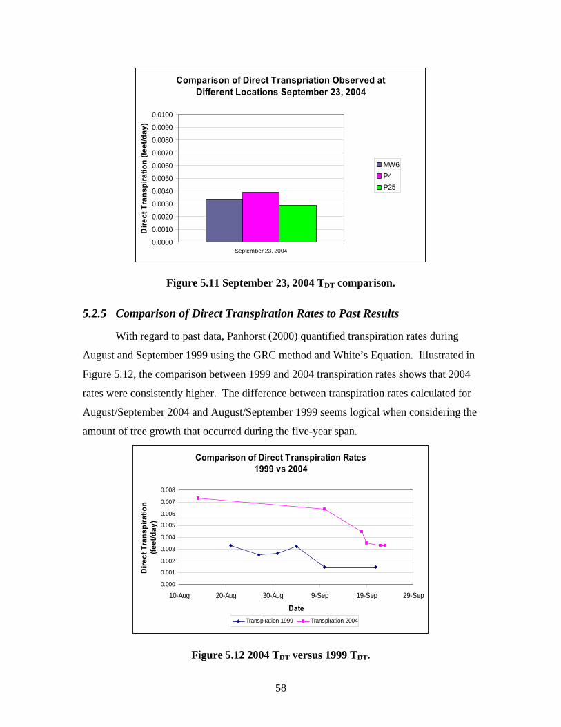
58

Comparison of Direct Transpriation Observed at Different Locations September 23, 2004

0.0000

0.0010

0.0020

0.0030

0.0040

0.0050

0.0060

0.0070

0.0080

0.0090

0.0100

September 23, 2004

Dire

ct T

rans

pira

tion

(feet

/day

)

MW6P4P25

Figure 5.11 September 23, 2004 TDT comparison.

5.2.5 Comparison of Direct Transpiration Rates to Past Results

With regard to past data, Panhorst (2000) quantified transpiration rates during

August and September 1999 using the GRC method and White’s Equation. Illustrated in

Figure 5.12, the comparison between 1999 and 2004 transpiration rates shows that 2004

rates were consistently higher. The difference between transpiration rates calculated for

August/September 2004 and August/September 1999 seems logical when considering the

amount of tree growth that occurred during the five-year span.

Comparison of Direct Transpiration Rates1999 vs 2004

0.000

0.001

0.002

0.003

0.004

0.005

0.006

0.007

0.008

10-Aug 20-Aug 30-Aug 9-Sep 19-Sep 29-Sep

Date

Dire

ct T

rans

pira

tion

(feet

/day

)

Transpiration 1999 Transpiration 2004

Figure 5.12 2004 TDT versus 1999 TDT.

59

Panhorst (2000) also performed a simple water budget for the Oneida

phytoremediation site using hydrologic data from 1998. The results of this water budget

yielded monthly volumetric evapotranspiration rates for a 1.67 acre area which comprised

the Oneida phytoremediation system and part of its surrounding area. When divided by

the area of the site (72,745.2 square feet), Panhorst’s values yield a time trend of

evapotranspiration rates which can be compared to direct transpiration rates calculated

for 2004. This comparison is illustrated in Figure 5.13.

Comparison of Direct Transpiration Values (2004) to Evapotransiration Values (1999)

0.0000

0.0020

0.0040

0.0060

0.0080

0.0100

0.0120

1-Jan 15-Feb 31-Mar 15-May 29-Jun 13-Aug 27-Sep 11-Nov 26-Dec

Day-Month

Evap

o/Tr

ansp

iratio

n (fe

et/d

ay)

MW6: Transpiration 2004 Evapotranspiration 1999

Figure 5.13 Comparison of 2004 TDT to 1999 ET.

The comparison between direct transpiration values calculated for the 2004 active

season and evapotranspiration values calculated for the 1999 season yields two primary

observations: 1) the transpiration time trends of water are similar in that there is an

increase between early spring and late spring, there is a decrease of water lost from the

site in mid-summer, an increase towards late summer, and a final decrease towards the

end of the active season; 2) the rate of water lost from the site during 1999 is consistently

lower than the rate lost from the site during 2004. With regard to first point, the time

trend of transpiration seems to agree with rainfall trends at the Oneida site. During the

early spring there are typically many rain events, during early summer there is a dry

period, there second wet period in late summer, and finally dry weather during early fall.

60

As illustrated in Figures 5.3-5.7, rainfall is directly related to saturated thickness. With

regard to the second point, if the rate of water lost is directly related to direct

transpiration by the hybrid poplar trees, it is logical that there was an increase in

[evapo]transpiration rates since there was tree growth between 1999 and 2004. Tree

diameter has been directly correlated with transpiration rates (Vose 2003, Calder 1993).

Corack (2000) also estimated the total volume of evapotranspiration from the site

using a detailed water budget analysis. Corack estimated the total volume of water lost

due to evapotranspiration from the site was equal to 141,800 ft3 during May 1999. The

area modeled was equal to 403,180 ft2. The daily evapotranspiration rate for the month

of May is determined by the following:

( ) dayft

ftdayft

ftAdayftQ

dayftET

dayft

daysft

daysftV

dayftQ

ET

May

MayETET

0113.0180,403

4.4548

4.454831

000,141#

2

3

2

3

333)(

3

==⎟⎟⎠

⎞⎜⎜⎝

⎛

=⎟⎟⎠

⎞⎜⎜⎝

⎛

===⎟⎟⎠

⎞⎜⎜⎝

⎛

The direct transpiration rates quantified for the month of May in 2004 were

determined by both the Groundwater Recession Comparison Method (MW6, P4) and

White’s Equation (P25). The direct transpiration rates determined during the month of

May for MW6, P4, and P25 are 0.0100, 0.0067, and 0.0081 feet/day, respectively. The

average of all of these values is 0.0083 feet/day. This value for direct transpiration is

slightly lower than the value of evapotranspiration determined by Corack (2000). This is

logical considering the value of evapotranspiration calculated by Corack included all

water both evaporated and transpired from the entire aquifer over the 403,180 ft3,

including both the saturated and vadose zones underlying the roughly 1-acre

phytoremediation system. This difference is logical considering the total ET should

always be greater than direct transpiration. However, it is evident from the calculation of

direct transpiration in 2004 that direct transpiration is the dominant quantity within the

ET value. It should be noted that the average value of evapotranspiration reported by

Corack for the entire growing season of 1999 was 0.0041 feet/day while for 2004 is was

61

0.0048 feet/day. This is also logical considering the trees grew significantly, thus

increasing the rate of direct transpiration, during that time period.

5.2.6 Comparison of Direct Transpiration at Oneida to Other Sites

In general, direct transpiration rates observed at the Oneida phytoremediation site

agreed with transpiration rates observed at other sites which included hybrid poplar

stands and hybrid poplar phytoremediation systems. For example, transpiration

measurements at a poplar stand in Flanders, Belgium yielded a daily maximum and mean

of 0.0164 and 0.0062 feet/day, respectively, between April 1st and October 31st

(Meiresonne et al, 1999). At the Oneida site, the daily maximum and mean observed was

0.0100 and 0.0048 feet/day, respectively. Poplar trees found at the Belgium site were 13

years old at the time of measurement, while at the Oneida site the trees were

approximately 9 years old. The majority of the trees found at the Belgium site had a

DBH of over one foot, while at Oneida the majority of the trees had a DBH between 0.10

and 0.40 feet. Trees at Oneida were spaced much closer than at the site in Belgium, 3

feet x 10 feet versus 23 feet x 24.6 feet, respectively.

Mid-summer transpiration rates for poplar based phytoremediation systems in

Texas, Colorado, and Florida were reported to be 0.0033, 0.0014, and 0.0062 feet/day

(Vose et al, 2003). At Oneida, mid-summer rates quantified from MW6 data (July and

August) were 0.0033 and 0.0073 feet/day respectively.

5.3 Estimation of Volumetric Direct Transpiration Rates

5.3.1 Results of Individual Tree Volumetric Transpiration Rates

The results of applying direct transpiration rates to representative areas

surrounding observation points MW6, P4, and P25 yielded individual volumetric direct

transpiration rates for 164 trees found within the three 900 and 2500 square-foot

representative areas. Using these volumetric direct transpiration rates from each

representative area, per tree volumetric direct transpiration rates (QTDT) were calculated

as shown in the example calculation in Table 4.3. Plots of per tree volumetric direct

transpiration for all of the 164 trees are shown in Appendix E.

62

5.3.2 Variation of the k-value

When plotted, values of per tree volumetric direct transpiration from each

representative area (900 and 2500 square-foot) versus tree diameter yield a k-value from

the power equation: QTDT = kx2 where x is the tree diameter and the units of coefficient k

are gal-ft/ft3-day so as to yield gallons/day using DBH in units of feet. A series of plots

showing the distribution of TDT values over a 900 square-foot area containing 19 trees for

MW6 from April through October 2004 is shown in Figures 5.14.

MW6: April 18, 2004, TDT=0.00431ft/day, 900 sq ft Area

y = 11.145x2

0.00

0.50

1.00

1.50

2.00

2.50

3.00

0.00 0.10 0.20 0.30 0.40 0.50 0.60

Tree Diameter (feet)

QT D

T (ga

l/day

)

MW6: May 6, 2004, TDT=0.00999 ft/day, 900 sq ft Area

y = 25.833x2

0.00

1.00

2.00

3.00

4.00

5.00

6.00

7.00

0.00 0.10 0.20 0.30 0.40 0.50 0.60

Tree Diameter (feet)

QT D

T (ga

l/day

)

MW6: June 6, 2004, TDT=0.0046 ft/day, 900 sq ft Area

y = 11.895x2

0.00

0.50

1.00

1.50

2.00

2.50

3.00

3.50

0.00 0.10 0.20 0.30 0.40 0.50 0.60

Tree Diameter (feet)

TDT (

gal/d

ay)

MW6: July 9, 2004, TDT=0.0064 ft/day, 900 sq ft Area

y = 8.5333x2

0.00

0.50

1.00

1.50

2.00

2.50

0.00 0.10 0.20 0.30 0.40 0.50 0.60

Tree Diameter (feet)

QT D

T (ga

l/day

)

MW6: August 14, 2004, TDT=0.0064 ft/day, 900 sq ft Area

y = 18.877x2

0.00

1.00

2.00

3.00

4.00

5.00

6.00

0.00 0.10 0.20 0.30 0.40 0.50 0.60

Tree Diameter (feet)

QT D

T (ga

l/day

)

MW6: September 10, 2004, TDT=0.0064 ft/day, 900 sq ft Area

y = 16.55x2

0.00

0.501.00

1.502.00

2.503.00

3.504.00

4.50

0.00 0.10 0.20 0.30 0.40 0.50 0.60

Tree Diameter (feet)

QT D

T (ga

l/day

)

Figure 5.14 Series of per tree volumetric direct transpiration versus tree diameter plots of trees within 900 ft2 area surrounding MW6.

63

The application of all direct transpiration rates from all observation points to 900 and

2500 square-foot representative areas yielded 44 k-values (Table 5.6). During 2004, k-

values ranged from 1.39 to 39.03 gal-ft/ft3-day.

Table 5.6 Tabulated k-values resulting from the application of direct transpiration rates to trees within representative areas surrounding observation points MW6, P4, and P25.

Observation Point

#

Date TDT (feet/day)

Representative Area: 900 ft2

k

Representative Area: 2500 ft2

k

MW6 3/23/04 0.0005 1.290 1.478 MW6 4/18/04 0.0043 11.145 13.850 MW6 5/6/04 0.0100 25.830 32.103 MW6 6/5/04 0.0046 11.895 14.782 MW6 7/9/04 0.0033 8.533 10.605 MW6 8/14/04 0.0073 18.877 23.459 MW6 9/10/04 0.0064 16.550 20.567 MW6 9/23/04 0.0033 8.533 10.605 MW6 10/3/04 0.0014 3.620 4.499

P4 4/4/04 0.0001 13.024 15.585 P4 4/27/04 0.0042 17.661 21.133 P4 5/5/04 0.0067 28.114 33.692 P4 6/7/04 0.0033 13.909 16.745 P4 9/18/04 0.0045 18.925 19.671 P4 9/22/04 0.0033 13.909 16.644 P4 9/23/04 0.0039 16.438 19.671

P25 3/7/04 0.0006 2.940 2.321 P25 4/2/04 0.0029 14.055 11.103 P25 4/21/04 0.0080 39.031 30.832 P25 5/4/04 0.0081 38.198 30.175 P25 9/19/04 0.0035 16.993 13.424 P25 9/23/04 0.0028 13.712 10.832

Since k-values are based on direct transpiration rates (feet/day) quantified by the

GRC method and White’s Equation, the time trend of k-values is similar to the time trend

for TDT values. Values of k were calculated at all observation points (MW6, P4, and P25)

for both 900 and 2500 square-foot representative areas. In general (73%), values of k

determined using a 2500 square-foot representative area were larger than k-values

determined using a 900 square-foot representative area. This difference can be attributed

to variation in the number of trees per unit area. As the number of trees per unit area

increases for a specified representative area, the value of k decreases. Conversely, as the

64

number of trees per unit area decreases for the same sized representative area, the value

of k increases. For instance, if the representative area was increased to 100,000 square

feet for all observation points, the representative area would contain all of the trees within

the phytoremediation system. Keeping in mind that volumetric transpiration is directly

proportional to land area (QDT = TDT x A), if the representative area continued to grow,

the number of poplar trees within the area would remain the same (finite number of

poplars), which would result in infinitely growing k-value. This leads to the question:

what representative area with what number of trees per unit area best represents the

Oneida phytoremediation site? That questioned can only be answered when the

boundaries of the phytoremediation site are determined. This study overlaid a 40,000

square foot grid to encompass the portion of the phytoremediation site which contains the

contaminant plume. Within the grid, the number of trees per square foot ranged from

approximately 0 to 0.05. The number of trees per square foot for the representative areas

used around each observation point is shown in Table 5.7.

Table 5.7 Number of trees per square foot within representative areas surrounding

each observation point.

Representative Area 900 sq-ft 2500 sq-ft Observation

Point # trees/sq-ft # trees/sq-ft

MW6 0.0211 0.0172

P4 0.0244 0.0252

P25 0.022 0.0232

The values shown in Table 5.7 are in good agreement with the average number of

trees per square foot found at the Oneida phytoremediation site, however the value for

MW6 using a 2500 square-foot area was somewhat low. This was expected because

there are fewer trees surrounding MW6. The number of trees per unit area surrounding

MW6 is lower because a portion of its 2500 square-foot area is occupied by the oil-water

separator and thus not planted.

65

With the assumption that the number of the trees found within the representative

areas surrounding each observation point are indicative of the entire site, the k-values

were lumped together so that an overall time trend of volumetric direct transpiration

could be observed. Figure 5.15 illustrates the time trend of k-values for both

representative areas using k-values calculated at all observation points during 2004. The

k-values are plotted with saturated thickness values determined from discrete water level

measurements and the average of continuous water levels observed during the calculation

of TDT.

Direct Transpiration Coefficient k Values from MW6, P4, P25 2004

0.0

5.0

10.0

15.0

20.0

25.0

30.0

35.0

40.0

M A M J J A S O

Month

QT D

T coe

ffici

ent,

k

2

3

4

5

6

7

8

9

10

k-900 sq ft k-2500 sq ft Sat Thick

Figure 5.15 Time trend of k-values from all observation points during 2004.

Since k-values are proportional to direct transpiration rates (feet/day), the time

trend is similar. Plotting k-values for both the 900 and 2500 square-foot representative

areas provided a range of k-values which can be applied to the entire phytoremediation

system to determine the volumetric direct transpiration of the system on a per tree basis.

The sum of the per tree volumetric transpiration rates will indicate the total volumetric

direct transpiration rate for the system.

66

5.3.3 Application of the k-value to Study Site Poplar Trees

Based on Figure 5.15, if the average k-value (900 and 2500 square feet) on a per

month basis is applied to all of the trees of the phytoremediation system, a range of per

tree volumetric transpiration rates on a monthly basis can be established. Figure 5.16

illustrates the distribution of volumetric transpiration over the range of tree sizes found at

the Oneida site on a monthly basis. During the month of peak transpiration (May), the

per tree volumetric direct transpiration values range from 0.26 gallons/day to just over 13

gallons/day during times of peak transpiration. During early October, the period of

lowest transpiration, the values ranged from 0.03 to 1.56 gallons/day. The large range of

per tree volumetric direct transpiration rates is attributed to the large range of tree

diameters found on-site.

0.61

-.64

0.41

-.50

0.21

-.30

0.03

-0.1

0 A M J J A S O0.00

2.00

4.00

6.00

8.00

10.00

12.00

14.00

Dire

ct T

rans

pira

tion

(gal

lons

/day

)

DBH (feet)

Month (2004)

Range of Direct Transpiration Rates Over TimeBased on Average Monthly k- coefficients

Figure 5.16 Distribution of volumetric direct transpiration over time based on DBH.

While the amount of water transpired by trees which are greater than 0.5 feet in

diameter looks significant, it should be noted that the percentage of trees within this

group is fewer than 2%. Trees which range from 0.21-0.30 feet in diameter make up

38% of this site, followed by range of 0.11-0.20 feet and 0.31-0.40 feet which make up

67

31.3% and 19.5%, respectively, of tree diameters on site. With regard to Figure 5.16, if

more of the trees were able to grow to their maximum potential, then the volumetric rate

of water directly transpired from the site would increase considerably.

5.3.4 Comparison of Volumetric Direct Transpiration to Past Results

In 2003, Corack calculated evapotranspiration for 1998 using the MODFLOW’s

ET package within GMS. Over an 8.5 day period for an area containing sixty trees

Corack calculated a minimum (based on the average of 60 trees) transpiration rate of 0.4

gallons/day-tree and a maximum rate of 5.3 gallons/day-trees. This range of per tree

transpiration rates by Corack is in good agreement with the rates determined in this study.

5.3.5 Comparison of Volumetric Direct Transpiration at Oneida to Other Sites

In general, volumetric direct transpiration rates estimated for the Oneida

phytoremediation site agreed with volumetric transpiration rates quantified at other sites.

At a phytoremediation system in Ogden, Utah, daily average volumetric transpiration

rates resulting from 3-year old hybrid poplar trees was 449 gallons/day (Ferro et al,

2001). Based on observed direct transpiration rates, the average volumetric direct

transpiration rate during 2004 at the Oneida site was estimated at 741 gallons/day.

Though the Oneida site value seems significant in comparison, the Ogden, Utah site had

only 25% as many trees as the Oneida site. Based on sap flow data, the Aberdeen,

Maryland site reported an average 1090 gallons/day an area which contained 171 hybrid

poplars. It should be noted that sap flow includes all water transpired from both the

vadose and saturated zone of an aquifer, while direct transpiration rates only pertain to

water from the saturated zone.

When the total daily volumetric transpiration rate is simply divided by the number

of living trees at the Oneida site, the average value for transpiration appears low (1.2

gallons/day-tree). However, it should be noted that many of the trees at Oneida have

very small diameters despite their age. The variation in tree diameter at Oneida ranges

from 0.03 feet to 0.64 feet, with the majority of the trees falling within the lower half of

that range. This relatively significant variation can probably be attributed to the

relatively tight spacing of the poplar trees at Oneida. Being a competitive species, the

larger poplar trees at the study site have thrived while smaller trees have grown very

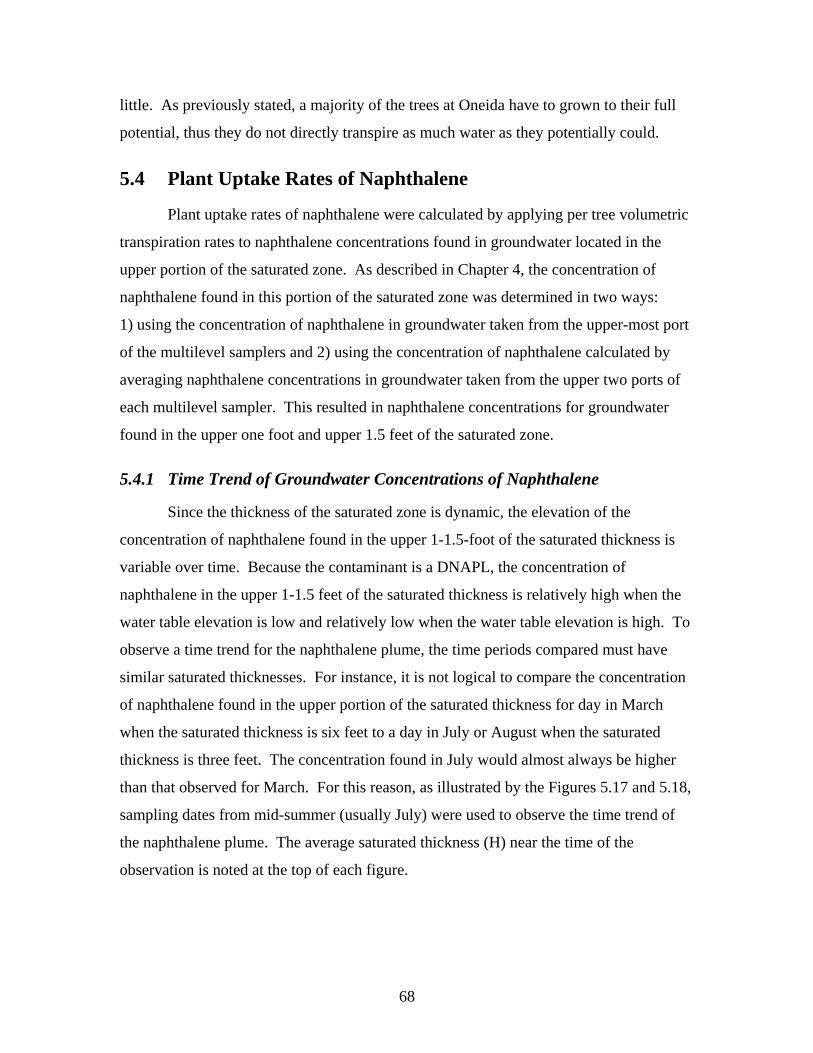
68

little. As previously stated, a majority of the trees at Oneida have to grown to their full

potential, thus they do not directly transpire as much water as they potentially could.

5.4 Plant Uptake Rates of Naphthalene

Plant uptake rates of naphthalene were calculated by applying per tree volumetric

transpiration rates to naphthalene concentrations found in groundwater located in the

upper portion of the saturated zone. As described in Chapter 4, the concentration of

naphthalene found in this portion of the saturated zone was determined in two ways:

1) using the concentration of naphthalene in groundwater taken from the upper-most port

of the multilevel samplers and 2) using the concentration of naphthalene calculated by

averaging naphthalene concentrations in groundwater taken from the upper two ports of

each multilevel sampler. This resulted in naphthalene concentrations for groundwater

found in the upper one foot and upper 1.5 feet of the saturated zone.

5.4.1 Time Trend of Groundwater Concentrations of Naphthalene

Since the thickness of the saturated zone is dynamic, the elevation of the

concentration of naphthalene found in the upper 1-1.5-foot of the saturated thickness is

variable over time. Because the contaminant is a DNAPL, the concentration of

naphthalene in the upper 1-1.5 feet of the saturated thickness is relatively high when the

water table elevation is low and relatively low when the water table elevation is high. To

observe a time trend for the naphthalene plume, the time periods compared must have

similar saturated thicknesses. For instance, it is not logical to compare the concentration

of naphthalene found in the upper portion of the saturated thickness for day in March

when the saturated thickness is six feet to a day in July or August when the saturated

thickness is three feet. The concentration found in July would almost always be higher

than that observed for March. For this reason, as illustrated by the Figures 5.17 and 5.18,

sampling dates from mid-summer (usually July) were used to observe the time trend of

the naphthalene plume. The average saturated thickness (H) near the time of the

observation is noted at the top of each figure.

69

June 1999 July 2000

July 2001 July 2002

August 2003 July 2004

Figure 5.17 Concentrations determined by averaging concentrations measured from the top 2 ports of each multilevel sampler.

H=4.45’ H=4.03’

H=3.27’

H=3.14’ H=4.45’

H=2.35’

70

June 1999 July 2000

July 2001 July 2002

August 2003 July 2004

Figure 5.18 Concentrations measured from top port of each multilevel samplers.

H=4.45’

H=2.35’

H=4.03’ H=4.45’

H=3.27’

H=3.14’

71

When the concentrations from the multilevel sampler locations were linearly

interpolated by GMS, a concentration was assigned to each cell. When averaged over the

entire grid, these concentrations were plotted to observe the time trend of naphthalene

concentrations found in the upper portion of the saturated thickness. Figure 5.19

illustrates a comparison between the average concentration of all the cells determined

from samples taken from the top port of each multilevel sampler and the average

concentration from samples derived from the top two ports of each multilevel sampler. It

can be observed from the comparisons shown in Figure 5.19 that the average of the

concentrations of naphthalene sampled from the upper two ports of the multilevel

samplers are consistently greater than the concentration of naphthalene sampled from

only the top port of the multilevel samplers. This difference is logical considering the

DNAPL, the source of the naphthalene, primarily exists on the bottom of the aquifer.

Average Concentration of Naphthalene in Upper Portion of Saturated ThicknessComparison Between Ports Sampled

0

200

400

600

800

1000

1200

1400

1999 2000 2001 2002 2003 2004

Date

Naph

thal

ene

Conc

(ug/

L)

Avg Top 2 Ports Top Port Only

Figure 5.19 Comparison of the average of the top two ports versus the top port only.

One of the objectives of this study is to determine the mass removal rate of

naphthalene from the groundwater underlying the study site. Using the concentration of

naphthalene found in each cell, the mass of naphthalene found in the upper 1-1.5 feet of

the saturated thickness was calculated by multiplying by the assumed porosity (n=0.3)

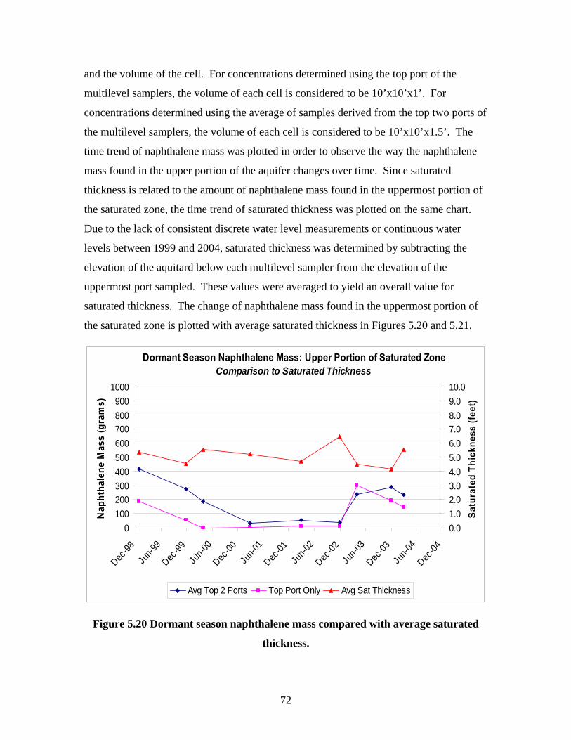
72

and the volume of the cell. For concentrations determined using the top port of the

multilevel samplers, the volume of each cell is considered to be 10’x10’x1’. For

concentrations determined using the average of samples derived from the top two ports of

the multilevel samplers, the volume of each cell is considered to be 10’x10’x1.5’. The

time trend of naphthalene mass was plotted in order to observe the way the naphthalene

mass found in the upper portion of the aquifer changes over time. Since saturated

thickness is related to the amount of naphthalene mass found in the uppermost portion of

the saturated zone, the time trend of saturated thickness was plotted on the same chart.

Due to the lack of consistent discrete water level measurements or continuous water

levels between 1999 and 2004, saturated thickness was determined by subtracting the

elevation of the aquitard below each multilevel sampler from the elevation of the

uppermost port sampled. These values were averaged to yield an overall value for

saturated thickness. The change of naphthalene mass found in the uppermost portion of

the saturated zone is plotted with average saturated thickness in Figures 5.20 and 5.21.

Dormant Season Naphthalene Mass: Upper Portion of Saturated ZoneComparison to Saturated Thickness

0100200300400500600700800900

1000

Dec-98

Jun-9

9Dec

-99Ju

n-00

Dec-00

Jun-0

1Dec

-01Ju

n-02

Dec-02

Jun-0

3Dec

-03Ju

n-04

Dec-04

Nap

htha

lene

Mas

s (g

ram

s)

0.01.02.03.04.05.06.07.08.09.010.0

Satu

rate

d Th

ickn

ess

(feet

)

Avg Top 2 Ports Top Port Only Avg Sat Thickness

Figure 5.20 Dormant season naphthalene mass compared with average saturated

thickness.

73

Active Season Naphthalene Mass: Upper Portion of Saturated ZoneComparison to Saturated Thickness

0100200300400500600700800900

1000

Dec-98

Jun-9

9

Dec-99

Jun-0

0

Dec-00

Jun-0

1

Dec-01

Jun-0

2

Dec-02

Jun-0

3

Dec-03

Jun-0

4

Dec-04

Nap

htha

lene

Mas

s (g

ram

s)

0.01.02.03.04.05.06.07.08.09.010.0

Satu

rate

d Th

ickn

ess

(feet

)

Avg Top 2 Ports Top Port Only Avg Sat Thickness

Figure 5.21 Active season naphthalene mass compared with average saturated

thickness.

Figures 5.20 suggests that during dormant months, when the water table is presumably

high due to recharge and lack of transpiration, the mass of naphthalene observed in the

uppermost portion of the saturated zone is relatively low. Conversely, during the active

months shown in Figure 5.21, when the water table is generally lower than in dormant

months, the concentration in the upper portion of the saturated zone is relatively high. It

is logical that the amount of naphthalene present in groundwater is higher when the water

table is lower since the source of the contaminant is closer to the bottom of the aquifer.

However, when observing summer months, Figure 5.21 show that naphthalene mass

found in the upper portion of the aquifer increases over time. This variation could be

attributed to an increase in direct transpiration over time. The effect of direct

transpiration from the saturated zone could create an upward flux of naphthalene towards

the upper portion of the aquifer. If this is true, then it seems logical that the rate of

naphthalene mass removal increase over time.

74

Depending on one’s perspective, an increase in naphthalene mass within the upper

portion of the saturated zone over time is not necessarily a desired trend with regard to

contaminant attenuation. However, if trees on site are directly transpiring contaminated

groundwater from upper portion of the saturate thickness and the mass of naphthalene

within that portion of the saturated thickness is increasing, then the mass removal of

naphthalene is increasing over time. This indicates an increased attenuation rate for

naphthalene removal from the subsurface.

With regard to this study, one problem with time trends is that they do not always

portray an accurate picture of what might actually be happening. For instance,

concentration data were generally measured on a bi-annual basis. Since determination of

the average saturated thickness is dependent on the elevation of the uppermost port

sampled from each multilevel sampler, the only “snapshots” in time for which saturated

thickness data are the same days which groundwater was sampled. It can be assumed that

the dissolution of naphthalene from the DNAPL to groundwater does not happen all at

once, but over time period during which the magnitude of the saturated thickness often

changes. It can be observed from groundwater data that the saturated thickness is subject

to numerous fluctuations due to recharge events. During these recharge events the

groundwater table rises and subsequently falls. These fluctuations assumedly change the

spatial location of naphthalene mass to some degree. Since recharge to the aquifer is a

direct result of rainfall events, the mass of naphthalene was compared to yearly rainfall

totals in Figures 5.22 and 5.23.

It can be observed in Figure 5.22 that the trend of yearly rainfall and naphthalene

mass in the upper portion of the saturated thickness both decrease over time. The mass of

naphthalene then remains relatively constant until 2003 when an increase occurs. During

the same time period, below average rainfall gradually returns to average in 2002 and

then exceeds average in 2003. Figure 5.23 suggests similar trends, but the correlation

between the mass of naphthalene found in the upper portion of the saturated thickness

and yearly rainfall totals is much more pronounced. It can be assumed that the more

often rain events occur, the more water fluctuations occur. This increase in water

fluctuations may increase the dissolution rate of naphthalene from the DNAPL to

groundwater. In addition, the increase of direct transpiration due to the growth of trees

75

and increased saturated zone availability may increase the upward flux of naphthalene

toward the upper portion of the saturated zone.

Dormant Season Naphthalene Mass: Upper Portion of Saturated ZoneComparison to Yearly Rainfall Totals

0100200300400500600700800900

1000

Dec-98

Jun-9

9Dec

-99Ju

n-00

Dec-00

Jun-0

1Dec

-01Ju

n-02

Dec-02

Jun-0

3Dec

-03Ju

n-04

Dec-04

Nap

htha

lene

Mas

s (g

ram

s)

30

40

50

60

70

80

Year

ly R

ainf

all T

otal

(inc

hes)

Avg Top 2 Ports Top Port Only Yearly Rainfall

Figure 5.22 Time trend of dormant season naphthalene mass and yearly rainfall.

Active Season Naphthalene Mass: Upper Portion of Saturated ZoneComparison to Yearly Rainfall Totals

0100200300400500600700800900

1000

Dec-98

Jun-9

9

Dec-99

Jun-0

0

Dec-00

Jun-0

1

Dec-01

Jun-0

2

Dec-02

Jun-0

3

Dec-03

Jun-0

4

Dec-04

Nap

htha

lene

Mas

s (g

ram

s)

30

40

50

60

70

80

Year

ly R

ainf

all T

otal

(inc

hes)

Avg Top 2 Ports Top Port Only Yearly Rainfall

Figure 5.23 Time trend of dormant season naphthalene mass and yearly rainfall.

76

Since plant uptake is dependent on the amount naphthalene found in the

groundwater and the amount of naphthalene found in the upper portion of the saturated

thickness is presumably dependent on the magnitude of the saturated thickness, then it

was logical to correlate the two. However, since the saturated thickness at the time of the

measurement of naphthalene concentrations was not precisely indicative of the trend of

the saturated thickness, it was also logical to correlate the amount of naphthalene found

in groundwater to yearly rainfall totals. Figures 5.24 and 5.25 illustrate these

correlations, respectively.

y = -88.993x + 647.85R2 = 0.3745

y = -67.785x + 496.23R2 = 0.1945

0

100

200

300

400

500

600

0.00 2.00 4.00 6.00 8.00 10.00

Saturated Thickness, H (feet)

Mas

sNap

htha

lene

, Upp

er P

ortio

n of

H,

(gra

ms) Active Season

Dormant SeasonLinear (Active)Linear (Dormant)

Figure 5.24 Mass of Naphthalene versus saturated thickness, H.

y = 9.0921x - 144.78R2 = 0.4915

y = 3.4711x - 37.329R2 = 0.0763

0

100

200

300

400

500

600

30 40 50 60 70 80

Yearly Rainfall (inches)

Mas

s N

apht

hale

ne, U

pper

Por

tion

of H

, (g

ram

s) Active SeasonDormant SeasonLinear(Active)Linear (Dormant)

Figure 5.25 Mass of naphthalene versus yearly rainfall totals.

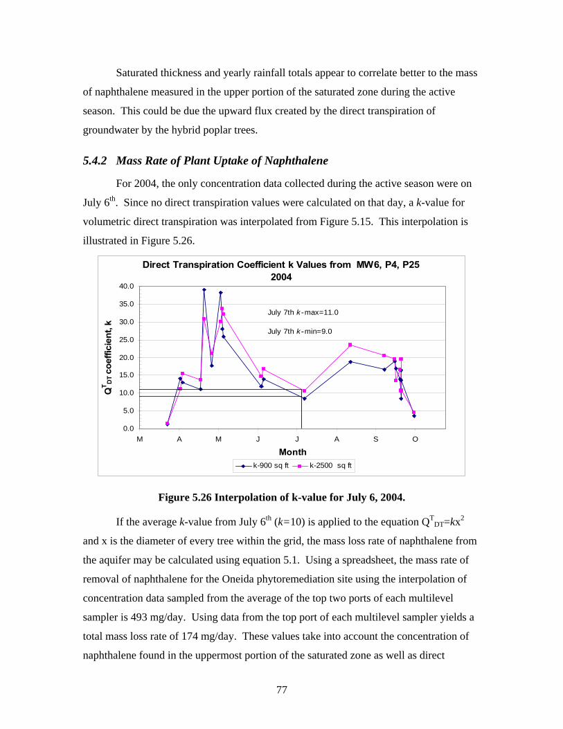
77

Saturated thickness and yearly rainfall totals appear to correlate better to the mass

of naphthalene measured in the upper portion of the saturated zone during the active

season. This could be due the upward flux created by the direct transpiration of

groundwater by the hybrid poplar trees.

5.4.2 Mass Rate of Plant Uptake of Naphthalene

For 2004, the only concentration data collected during the active season were on

July 6th. Since no direct transpiration values were calculated on that day, a k-value for

volumetric direct transpiration was interpolated from Figure 5.15. This interpolation is

illustrated in Figure 5.26.

Direct Transpiration Coefficient k Values from MW6, P4, P25 2004

0.0

5.0

10.0

15.0

20.0

25.0

30.0

35.0

40.0

M A M J J A S O

Month

QT D

T coe

ffici

ent,

k

k-900 sq ft k-2500 sq ft

July 7th k-max=11.0

July 7th k-min=9.0

Figure 5.26 Interpolation of k-value for July 6, 2004.

If the average k-value from July 6th (k=10) is applied to the equation QTDT=kx2

and x is the diameter of every tree within the grid, the mass loss rate of naphthalene from

the aquifer may be calculated using equation 5.1. Using a spreadsheet, the mass rate of

removal of naphthalene for the Oneida phytoremediation site using the interpolation of

concentration data sampled from the average of the top two ports of each multilevel

sampler is 493 mg/day. Using data from the top port of each multilevel sampler yields a

total mass loss rate of 174 mg/day. These values take into account the concentration of

naphthalene found in the uppermost portion of the saturated zone as well as direct

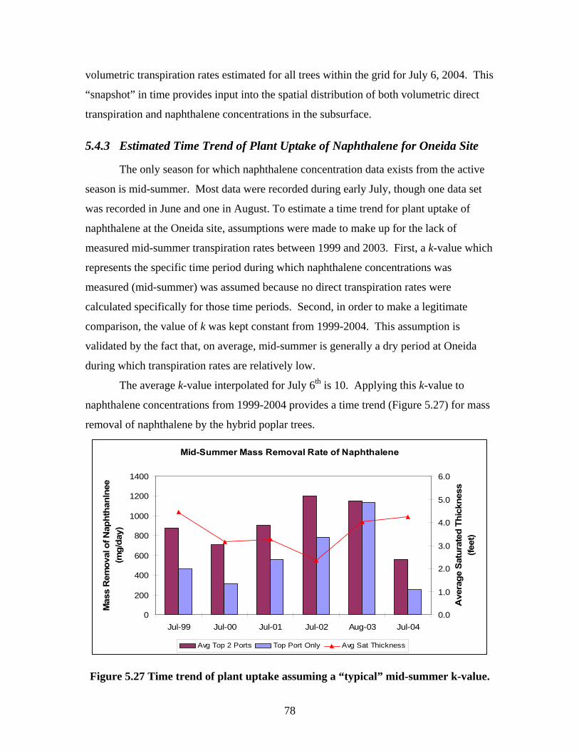
78

volumetric transpiration rates estimated for all trees within the grid for July 6, 2004. This

“snapshot” in time provides input into the spatial distribution of both volumetric direct

transpiration and naphthalene concentrations in the subsurface.

5.4.3 Estimated Time Trend of Plant Uptake of Naphthalene for Oneida Site

The only season for which naphthalene concentration data exists from the active

season is mid-summer. Most data were recorded during early July, though one data set

was recorded in June and one in August. To estimate a time trend for plant uptake of

naphthalene at the Oneida site, assumptions were made to make up for the lack of

measured mid-summer transpiration rates between 1999 and 2003. First, a k-value which

represents the specific time period during which naphthalene concentrations was

measured (mid-summer) was assumed because no direct transpiration rates were

calculated specifically for those time periods. Second, in order to make a legitimate

comparison, the value of k was kept constant from 1999-2004. This assumption is

validated by the fact that, on average, mid-summer is generally a dry period at Oneida

during which transpiration rates are relatively low.

The average k-value interpolated for July 6th is 10. Applying this k-value to

naphthalene concentrations from 1999-2004 provides a time trend (Figure 5.27) for mass

removal of naphthalene by the hybrid poplar trees.

Mid-Summer Mass Removal Rate of Naphthalene

0

200

400

600

800

1000

1200

1400

Jul-99 Jul-00 Jul-01 Jul-02 Aug-03 Jul-04

Mas

s R

emov

al o

f Nap

htha

nlne

e (m

g/da

y)

0.0

1.0

2.0

3.0

4.0

5.0

6.0

Ave

rage

Sat

urat

ed T

hick

ness

(fe

et)

Avg Top 2 Ports Top Port Only Avg Sat Thickness

Figure 5.27 Time trend of plant uptake assuming a “typical” mid-summer k-value.

79

Perhaps the most apparent trend observed in Figure 5.27 is the increase of

naphthalene mass removal over time. Keeping the volumetric direct transpiration rate

constant illustrates that rate of removal is dependent on the naphthalene concentration

found in the uppermost portion of the saturated thickness. As previously mentioned, the

concentration of naphthalene found in the uppermost portion of the saturated thickness

could be due to increased water table fluctuations caused by increased recharge events

and/or by an upward flux of naphthalene caused by the increased direct transpiration of

water from the saturated zone.

5.5 Plans and Profiles of Water Table Elevation Data

Using AutoCAD, plans and profiles of water table elevation data calculated using

discrete water level measurements were plotted so that the water table elevation and

saturated thickness could be compared on a month-to-month basis. The purpose of these

plots was to observe the time trend of the entire water table surface beneath the

phytoremediation system.

5.5.1 Cone of Depression

At other phytoremediation sites such as the one at Aberdeen, Maryland, a cone of

depression has been observed when examining groundwater contours during the active

season. At the Oneida site, a cone of depression was not apparent. One reason is due to

the number and placement of the piezometers which are used to measure the elevation of

the water table. All of the piezometers associated with the phytoremediation system are

relatively close to or within the system of trees. In order to observe a cone of depression,

the water table would have to be mapped well beyond the boundary of the

phytoremediation system. The inability to determine a cone of depression is illustrated

by contours for July 6th in Figure 5.28.

80

Figure 5.28 Plan view of water table contours for data measured on July 6, 2004.

5.5.2 Change of Hydraulic Profile over Time

In order to better determine the hydraulic nature of the aquifer underlying the

phytoremediation system, monthly profiles of the water table are compared. Earlier in

this study, it was observed from Figure 5.3 that groundwater fluctuations due to rain

events at P3 had a greater magnitude because there were hardly any trees surrounding

that location, thus there was less direct transpiration occurring in that area. Figures 5.29-

5.31 illustrate comparisons of the water table profile between different months during

2004. It should be noted that the left-hand side of the water table profiles begins

northwest of P3 in an area with no trees. The profile enters the treed area at station 00+75

and continues underneath the trees until intersecting P9.

81

Figure 5.29 Comparison of water table profiles for March, April, and May.

In Figure 5.29 the profile from March is the only observed profile from the

dormant season. The profile exhibits an entirely different character than the profiles

observed during the active season. During the active season, there is an obvious dip

beneath the area of the phytoremediation system which contains trees. This dip is

observed throughout the entire course of the active season (April through September).

In the final comparison between September and October (Figure 5.31), the

October profile is observed to be slightly higher than that observed for September. It

should be noted that September 2004 exhibited twice as much rainfall than October 2004,

7.58 inches versus 3.56 inches, respectively, but also had significantly higher direct

transpiration rates. The higher level of the groundwater table in October, the month

which received significantly less rain, suggests that the area beneath the trees is

influenced by the hybrid poplars more than the area just outside the area beneath the

82

trees. This is due to the fact that in October, the trees were hardly transpiring due to lack

of foliage.

Figure 5.30 Comparison of water table profiles for June, July, and August.

83

Figure 5.31 Water table profiles for September and October.

84

6 SUMMARY AND CONCLUSIONS Several studies have been conducted by Virginia Tech to evaluate the various

contaminant attenuation mechanisms of the Oneida phytoremediation system. One

mechanism, plant uptake, refers to the “root sorption, uptake, translocation, metabolic

transformation, and/or phytovolatilization” of organic chemicals from groundwater

(Schnoor, 2002). Plant uptake is a process known to remove contaminant mass from the

subsurface. Two significant components of plant uptake are direct transpiration of

groundwater and the aqueous concentration of contaminants in groundwater (Vose et al,

2003). Assessment of the seasonal and spatial variability of these components provides

an understanding of the plant uptake process which in turn can be used to more

thoroughly evaluate the effectiveness of the phytoremediation system.

The primary objectives of this research were: 1) to determine direct transpiration

rates (TDT) at the phytoremediation study site, 2) to estimate per tree volumetric direct

transpiration rates (QTDT), and 3) apply per tree volumetric direct transpiration rates to

concentration data to quantify the mass removal rate of naphthalene. Direct transpiration

rates were calculated for the 2004 growing season by analyzing water table recessions

and were validated by comparison to values of evapotranspiration and transpiration

calculated during previous site studies between 1999 and 2002 (Panhorst, 2000, Corack,

2003). Utilizing direct transpiration rates, per tree volumetric direct transpiration rates

were estimated under the assumption that variability in transpiration rates between trees

is directly correlated to tree diameter (Calder, 1993, Vose et al, 2003). Determination of

plant uptake rates of naphthalene was accomplished by applying per tree volumetric

direct transpiration rates and naphthalene concentration data to the equation for plant

uptake of organic chemicals by hybrid poplars (Briggs et al, 1983, Burken and Schnoor,

1998).

6.1 Summary of Findings

6.1.1 Quantification of Direct Transpiration Rates

Direct transpiration rates were quantified from three observation points within the

phytoremediation system at various times during the 2004 growing season. In all, 22

85

values of direct transpiration were calculated between March and October 2004. The

daily maximum and mean values for direct transpiration at the study site were 0.0100 and

0.0048 feet/day, respectively. Direct transpiration rates determined for the Oneida

phytoremediation site were in good agreement with transpiration rates determined at

other sites which utilized hydrologic, groundwater, and sap flow analysis (Meiresonne et

al, 1999, Schneider et al, 2002, Vose et al, 2003). Direct transpiration rates increased

between early spring and mid-spring in conjunction with an increase in tree foliation. As

shown by continuous groundwater level monitoring and water table profiles, the saturated

thickness, which was relatively high prior to the active season, decreased with the arrival

of spring and remained relatively low and steady throughout the active season. The

relatively and consistently low water table throughout the active season was attributed to

direct transpiration as well as interception resulting from transpiration of recharge water

in the vadose zone. Direct transpiration decreased during early summer. Though

assumed to be the peak of the growing season, an unexpected decrease in direct

transpiration was observed during early and mid-summer. This decrease was attributed

to below average rainfall observed in June which resulted in a relatively long period of

decline of the water table. Studies indicate that poplar trees may experience stress as a

result of water table decline (Mahoney, 1991). Symptoms of tree stress include a loss of

leaves and decreased transpiration rates, both of which were observed during mid-

summer. Direct transpiration rates and saturated thickness increased during August and

September in conjunction with rainfall events which occurred during that time period.

By early October nearly all of the leaves had fallen from the trees, the magnitude of the

saturated thickness had begun to increase, and direct transpiration rates had declined

considerably.

6.1.2 Estimation of Volumetric Transpiration

Per tree volumetric transpiration rates were estimated by multiplying observed

direct transpiration rates by representative areas around each observation point and

distributing that quantity amongst the trees found within the representative areas.

Plotting per tree volumetric direct transpiration (gallons/day-tree) versus tree diameter

(feet) yielded the power equation QTDT=kx2 where k was the volumetric direct

86

transpiration coefficient (gal-ft/ft3) and x was the tree diameter. Since the number of

trees within representative areas surrounding each observation point was determined to

correspond with phytoremediation system as a whole, values of k were applied to all trees

found on-site and summed to calculate total volumetric direct transpiration for the

phytoremediation system. The peak and average volumetric direct transpiration rates

during 2004 were 1750 and 750 gallons/day, respectively. These volumetric direct

transpiration rates were in good agreement with evapotranspiration and transpiration rates

quantified during previous Oneida phytoremediation site studies (Panhorst, 2000; Corack,

2003).

Estimation of per tree volumetric direct transpiration was based on the assumption

that variation in these rates is due to variation of the square of the tree diameter. Trees

which were all planted over the course of 1997 ranged from 0.03 to 0.64 feet in diameter.

This relatively large variation in diameter of trees which were approximately the same

age accounted for the variability of per tree direct transpiration rates. The maximum and

average tree diameter observed in 2004 was 0.64 and 0.25 feet, respectively. The daily

maximum and mean volumetric direct transpiration rate for average sized trees was 2.48

and 1.05 gallons/day, respectively. The daily maximum and mean volumetric

transpiration rate for the maximum sized trees was 15.81 and 6.69 gallons/day,

respectively. Direct transpiration rates were in good agreement with transpiration rates of

the Aberdeen, Maryland phytoremediation site which were reported to range from 1.4 to

10.8 gallons/day-tree over the course of the season (Schneider et al, 2003). Per tree

estimates of volumetric direct transpiration calculated for the Oneida site were also in

good agreement with sap flow rates measured at other phytoremediation sites located in

Texas, Colorado, and Florida (Vose et al, 2003).

Hinckley reported that 4-year old poplar trees transpire between 5.3 and 6.9

gallon/day based on sap flow measurements (1994). In January 2001, when the trees at

the Oneida study site were roughly 4 years old, the maximum tree diameter was 0.41 ft.

From direct transpiration rates calculated during 2004, the average and maximum daily

volumetric transpiration rate for a tree of this size was 2.79 and 6.59 gallons/day.

Considering Hinckley measured sap flow, the amount water transpired from both the

87

vadose zone and the saturated zone, values calculated in this study appear to agree

favorably.

6.1.3 Quantification of Naphthalene Removal via Direct Transpiration

The mass removal rate of naphthalene from the aquifer underlying the Oneida

phytoremediation site was calculated by applying per tree volumetric direct transpiration

rates to local naphthalene concentrations sampled July 6, 2004. The mass removal of

naphthalene calculated for the entire plume area ranged from 174 to 493 mg/day on the

specified date. If the mass of naphthalene found in the upper portion of the aquifer

represents the amount of naphthalene found in the aqueous plume, then the amount of

naphthalene removed on July 6, 2004 constitutes from 0.06 to 0.17 percent of the

aqueous plume mass. When the per tree volumetric transpiration rates estimated for July

6, 2004 were applied to mid-summer naphthalene concentrations from previous years, the

time trend indicated that mass removal rate of naphthalene was generally increasing over

time. This increase was in conjunction with an increase in yearly rainfall totals.

Due to dependence on groundwater concentration, mass removal rates of

naphthalene vary over the course of the active season due to variation of direct

transpiration rates and concentrations of naphthalene in the upper portion of the saturated

thickness. Though the concentration of naphthalene found in the upper portion of the

saturated zone varies with the magnitude of the saturated thickness, it is expected that

other variables such as direct transpiration also influence the variability of naphthalene

concentrations.

6.2 Conclusions

Transpiration, a significant component of plant uptake at phytoremediation

systems, refers to water removed from the subsurface (vadose zone and saturated zone)

through live plants, while the term direct transpiration refers to water specifically from

the saturated zone. This study indicates the Groundwater Recession Comparison method

may be used to quantify the rate of direct transpiration from the saturated zone of a

shallow, unconfined aquifer which underlies a developed stand of phreatophytes.

White’s Equation may be utilized for the same purpose since evaporation may be ruled a

88

minor component of evapotranspiration when the canopy of the tree stand is full and the

depth to water from the land surface exceeds two feet (White, 1932, Freeze and Cherry,

1979, Vose and Swank, 1992). As opposed to evapotranspiration or total transpiration

from both the vadose zone and the saturated zone, direct transpiration from the saturated

zone plays an important role when evaluating the effectiveness of a DNAPL-

contaminated phytoremediation system since the trees “must transpire enough water from

the groundwater layer containing the pollutant to control the transport or decrease the

mass of the contaminant” (Vose et al, 2003). The results of this study showed that direct

transpiration rates varied considerably over the course of the growing season in response

to changes in climatic parameters, leaf area, and depth to water.

To quantify the mass removal rate of aqueous naphthalene, the spatial variability

of direct transpiration rates must be carefully considered. Variation in per tree direct

transpiration rates was attributed to differences in tree diameter (Vose et al, 2003). Direct

transpiration rates were distributed amongst trees within representative areas based on the

square of the diameter at breast height and extrapolated to the entire stand of hybrid

poplars (Calder, 1993). Accounting for variations in tree diameter proved to be

significant due to the wide range of tree diameters found within the phytoremediation

system.

Spatial variation in the concentration of contaminants in groundwater was also

considered. Naphthalene concentrations in the upper portion of the saturated zone varied

over time space due to changes in the magnitude of the saturated thickness. By

superimposing per tree volumetric direct transpiration rates over the aqueous naphthalene

plume and applying the equation for plant uptake for hybrid poplars by Burken and

Schnoor, the mass removal of naphthalene from the aquifer was calculated. The single

day mass removal estimate constituted approximately 0.12 % of the aqueous plume mass.

If the volumetric direct transpiration rate and the concentration of naphthalene remained

constant over time, the time to complete attenuation of naphthalene by plant uptake

would be approximately 833 days. Since plant uptake only occurs during the growing

season (generally considered 150 days), this would equate to roughly 5.5 years.

The effectiveness of plant uptake is limited by the relationship of direct

transpiration and naphthalene concentrations to the magnitude of the saturated thickness.

89

When the saturated thickness is great enough for direct transpiration to be maximized, the

concentration of naphthalene found in the uppermost portion of the saturated zone is

usually relatively low. Conversely, when the saturated thickness is in a state of decline

and the naphthalene concentrations are relatively high, direct transpiration is generally

minimized. This inversely proportional relationship suggests the efficiency plant uptake

of is not ideal at the phytoremediation site.

6.3 Future Considerations

In order to help substantiate per tree volumetric direct transpiration rates

estimated for the Oneida study site, sap flow analysis should be performed on some of the

hybrid poplars. Ideally, sap flow analysis would occur on trees found within a specific

representative area surrounding one of the piezometers used for direct transpiration rate

calculation. It would be interesting to observe how sap flow correlates to direct

transpiration and compare those results with the time trend of direct transpiration rates,

saturated thickness, and recharge events.

In order to predict the time to attenuation for naphthalene contamination, GMS

should be used to estimate the entire mass of naphthalene found within the saturated

thickness. Only by observing the decrease in mass found in the entire saturated thickness

can a determination be made regarding the effectiveness of the phytoremediation system

with regard to attenuation of contaminants.

Consideration should be given to the spacing of the hybrid poplar trees at the

Oneida phytoremediation site. If the trees were thinned, many more trees would be able

to grow to their maximum potential. The resulting increased root depth would allow more

direct transpiration of groundwater containing higher concentrations of naphthalene.

This would effectively increase the rate at which naphthalene mass is being removed.

90

7 REFERENCES Burken, J.G., J.L. Schnoor. Predictive Relationships for Uptake of Organic Contaminants

by Hybrid Poplar Trees. Environmental Science Technology. 32:3379-3385 (1998).

Briggs, G.G.; Bromilow, R.H.; Evans, A.A.; Williams, M. Relationships Between

Lipophilicity and the Distribution of Non-ionised Chemicals in Barley Shoots Following Uptake by the Roots. Pestic. Sci. 14 (1983).

Calder, I.R., M.H. Swaminath, G.S. Kariyappa, N.V. Srinivasalu, J. Mumtaz.1992.

Measurement of Transpiration from Eucalyptus Plantations, India, Using Deuterium Tracing. Growth and Water Use of Forest Plantations. John Wiley & Sons, New York, 1992.

Corack, E.J. 2003. Impact of Phytoremediation System on Groundwater Flow in a

Shallow Aquifer. Master’s Thesis. Virginia Polytechnic Institute and State University.

Cramer, V.A., P.J. Thorburn, G.W. Fraser. 1999. Transpiration and groundwater uptake

from forest plots of Casuarina glauca and Eucalyptus camaldulensis in saline areas of southeast Queensland, Australia. Agricultural Water Management, 39 (1999) 187-204.

Davis, G.B. and A.J. Peck.1986. Estimating evapotranspiration by analysis of bore

hydrographs. IAHS Publ. 156, 313-321. Eamus, D., A.P. O’Grady, L. Hutley. 2000. Dry season conditions determine wet season

water use in the wet–tropical savannas of northern Australia. Tree Physiology, 20: 1219-1236.

Ferro, A., J. Chard, R. Kjelgren, B. Chard, D. Turner, and T. Montague. 2001.

Groundwater Capture Using Hybrid Poplar Trees: Evaluation of a System in Ogden, Utah. Int. J. Phytoremediation. Vol. 3, no. 1, pp. 87-104. 2001.

Freeze, R.A. and J.A. Cherry. 1979. Groundwater. Prentice-Hall, New Jersey. Fitter, A.H. and R.K.M. Hay. 1981. Environmental Physiology of Plants. Academic

Prees, New York.

Garratt, J.R. 1984. The Measurement of Evaporation by Meteorological Methods. Agricultural Waste Management, 8 (1984) 99-117.

91

Hare, P.W. and R.E. Morse. 1997. Water-level fluctuations due to barometric pressure changes in an isolated portion of an unconfined aquifer. Ground Water, July 01, 1997.

Hillel, D. 1982. Hillel Introduction to Soil Physics, Academic Press, New York (1982). Hinckley, T.M., Brooks, J.R., Cermak, J., Ceulemans, R., Kucera, J., Meinzer, F.C.,

Roberts, D.A., 1994. Water Flux in a Hybrid Poplar Stand. Tree Physiology. 14, 1005-1018.

Hopkins, W.G. and N.P. Huner. 2004. Introduction to Plant Physiology, 3rd Ed. Wiley &

Sons, Inc., New York.

Husch, B., C. I. Miller and T. W. Beers. 1993. Forest Mensuration. Third Edition. Krieger Publishing Co., Malabar, Florida 402 p.

Jordahl, J.L., Foster, L., Schnoor, J.L., Alvarez, P.J.J., 1997.

Effect of hybrid poplar trees on microbial populations important to hazardous waste bioremediation. Environ.Toxicol. Chem. 16, 1318–1321.

Kjelgaard, J.F., 1996. Measuring sap flow with the heat balance approach using

constant and variable heat inputs. Agricultural and Forest Meteorology. 85 (1997) 239-250.

Lawrence, Matthew S. Spatial and Temporal Growth Trends of Poplar Trees Planted for

the Purpose of PAH Remediation. M.S. Thesis, Virginia Tech, June 2000.

Mahoney, J.M. and S.M. Brood. 1991. Response of a hybrid poplar to water table decline in different substrates. Department of Biological Sciences, University of Lethbridge, Lethbridge, Alta. T1K 3M4, Canada.

Meiresonne, L., N. Nadezhdin, J. Cermak, J.V. Slycken, and R. Ceulemans. 1999.

Measured sap flow and simulated transpiration from a poplar stand in Flanders (Belgium). Agricultural and Forest Meteorology. 96 (1999) 165-199.

Monteith, J.L., 1965. Evaporation and environment. In: Fogg, G. (Ed.), The State and Movement of Water in Living Organisms. Proceedings of the XIXth Symposium on the Society of Experimental Biology, Cambridge University Press, Cambridge, UK, pp. 205–234.

Noggle, R.G. and J.F. Fritz. 1976. Introduction to Plant Physiology. Prentice-Hall, Inc.,

New Jersey. Panhorst, E.M. 2000. Evapotranspiration Measurement and Simulation due to Poplar

Trees at a Phytoremediation Site. Master’s Thesis. Virginia Polytechnic Institute and State University.

92

Pivetz, B.C., 2001. Phytoremediation of contaminated soil and ground water at

hazardous waste sites. Office of Research and Development, US-EPA, EPA/540/S-01/500.

Schiller, G., 2001. Estimating the water use of sclerophyllous species under and East

Mediterranean climate. Forest and Ecology Management. 170 (2002) 117-126. Schneider, W.H., R.F. Weston, S.R. Hirsh, H.R. Compton. 2002. Analysis of Hydrologic

Data to Evaluate Phytoremediation System Performance. Journal of Phytoremediation.

Schnoor, J.L., 2002. Phytoremediation of Soil and Groundwater. Technology Evaluation

Report TE-02-01. Prepared for Ground-Water Remediation Technologies Analysis Center, Pittsburgh, PA.

Thornthwaite, C.W., 1948. An approach toward a rational classification of climate.

Geogr. Rev. 38, 55–94. Viessman W.and G.L. Lewis. 2003. Introduction to Hydrology, 5th ed. Harper-Collins,

New York. U.S. Environmental Protection Agency (EPA). 2000. Introduction to Phytoremediation.

Office of Research and Development Technical Report, EPA 1600/R-99/i 07, National Risk Management Laboratory, Cincinnati, OH.

Vose, J.M., G. Harvey, K. Elliot, B. Clinton. 2003. Measuring and Modeling Stand Level

Transpiration. Phytoremediation: Transformation and Control of Contaminants, Wiley & Sons, Inc., New York, pp.263-281.

Vose, J.M. and W.T. Swank. 1992. Water Balances. In: Atmospheric Deposition and

Forest Nutrient Cycling: A Synthesis of the Integrated Forest Study. D.W. Johnson and S.E. Lindberg, Ecological Studies 91, Springer-Verlag, New York, 27-49.

White, W.N. 1932. A Method of Estimating Ground-Water Supplies Based on Discharge

by Plants and Evaporation from Soil, Results of Investigations in Escalante Valley, Utah. U.S. Geological Survey Water-Supply Paper 659-A, 165p.

Zhang, H.and L.P. Simmonds.1997. Estimation of transpiration by single trees:

comparison of sap flow measurements with a combination equation. Agricultural and Forest Meteorology 87 (1997) 155-169.