Sains Malaysiana 46(10)(2017): 2007–2017 http://dx.doi.org/10.17576/jsm-2017-4610-40

Differential Transformation Method (DTM) for Solving SIS and SI Epidemic Models(Kaedah Transformasi Pembezaan (DTM) untuk Menyelesaikan Model Epidemik SIS dan SI)

M.Z. AHMAD*, D. ALSARAYREH, A. ALSARAYREH & I. QARALLEH

ABSTRACT

In this paper, the differential transformation method (DTM) is employed to find the semi-analytical solutions of SIS and SI epidemic models for constant population. Firstly, the theoretical background of DTM is studied and followed by constructing the solutions of SIS and SI epidemic models. Furthermore, the convergence analysis of DTM is proven by proposing two theorems. Finally, numerical computations are made and compared with the exact solutions. From the numerical results, the solutions produced by DTM approach the exact solutions which agreed with the proposed theorems. It can be seen that the DTM is an alternative technique to be considered in solving many practical problems involving differential equations.

Keywords: Differential transformation method (DTM); exact solution; semi-analytical solution; SIS model; SI model

ABSTRAK

Dalam kajian ini, kaedah transformasi pembezaan (DTM) telah digunakan untuk mencari penyelesaian separuh-analisis bagi model epidemik SIS dan SI untuk populasi malar. Pertama, latar belakang teori DTM telah dikaji dan diikuti dengan membina penyelesaian bagi model epidemik SIS dan SI. Selain itu, analisis konvergensi DTM telah dibuktikan melalui cadangan dua teorem. Akhir sekali, pengiraan berangka dibuat dan dibandingkan dengan penyelesaian tepat. Daripada keputusan berangka, penyelesaian yang diperoleh melalui DTM adalah hampir sama dengan penyelesaian tepat yang bersetuju dengan teorem yang dicadangkan. Boleh dikatakan bahawa DTM adalah satu teknik alternatif yang boleh dipertimbangkan untuk menyelesaikan banyak masalah praktikal yang melibatkan persamaan pembezaan.

Kata kunci: Kaedah transformasi pembezaan (DTM); model SIS; model SI; penyelesaian tepat; penyelesaian separuh-analitik

INTRODUCTION

There are many methods to solve differential equations. One of them is the Taylor series. The Taylor series, however, requires huge effort in order to find the derivatives of function. Moreover, it is very complicated to find the higher order derivatives of function. Due to these reasons, Zhou (1986) had proposed a new form of the Taylor series called the differential transformation method (DTM) and applied it to solve mathematical problems in electrical circuit analysis. The idea of the DTM is to determine the coefficients of the Taylor series of a function by solving the induced recursive equation from the given differential equation. The emergence of DTM has motivated many researchers to solve different types of differential equation. Chen and Ho (1996) had used it to construct the solution of partial differential equations while Jang and Chen (1997) had used the DTM to solve initial and boundary value problems. Later, Chen and Liu (1998) had employed this method to find the solution of two point boundary value problems. Next, Ayaz (2004) had constructed the solution of system of differential equations using DTM. In 2005, Abbasov and Bahadir (2005) had obtained semi-analytical solutions of linear and non-linear problems in engineering using the DTM. Hassan and Ertürk (2007) had used DTM to solve an

elliptic partial differential equation. Later, Hassan (2008) had used this method to solve linear and non-linear system of differential equations. Due to its popularity in solving various types of equation, many authors had used the DTM to solve difference equations (Arikoglu & Ozkol 2006), fractional differential equations (Arikoglu & Ozkol 2007; Momani et al. 2008), volterra integral equations (Odibat 2008; Tari et al. 2009), integro-differential equations of fractional order (Nazari & Shahmorad 2010), Burgers and Schrödinger equations (Abazari & Borhanifar 2010; Borhanifar & Abazari 2011), fractional chaotic dynamical systems (Alomari 2011) and partial differential equations of order four (Soltanalizadeh & Branch 2012). These contributions showed that the DTM is widely used to solve many types of differential equation as stated. In finding the solutions of SIS and SIR epidemic models (Kermack & McKendrick 1927), many studies have been attempted. Nucci and Leach (2004) had used Lie group to present the explicit solution of SIS epidemic model while Khan et al. (2009) had solved SIS and SIR epidemic models by means of homotopy analysis method (HAM). Later, Shabir et al. (2010) had proposed exact solutions of SIR and SIS epidemic models. In 2013, Abubakar et al. had obtained approximate solution of SIR model using homotopy perturbation method (HPM). Many efforts have

2008

been given to solve the SIS and SIR epidemic models by several researchers (Jing & Zhu 2005; Korobeinikov & Wake 2002; Pietro 2007; Yicang & Liu 2003; Zhien et al. 2003). Certain epidemiology models have been solved by DTM (Akinboro et al. 2014; Batiha & Batiha 2011). Batiha and Batiha (2011) considered the numerical solution of SIR model without vital dynamics using DTM, meanwhile Akinboro et al. (2014) considered the numerical solution of SIR model with vital dynamics using DTM. However, to the best of our knowledge, SIS model without vital dynamics and SI model with vital dynamics are not solved by DTM yet. Therefore, this paper focused on finding semi-analytical solutions of the SIS model without vital dynamics and SI model with vital dynamics using DTM. This paper is organized in the following sequence. Next, some basic definitions and fundamental properties of the DTM are introduced, followed by constructing semi-analytical solutions of the SIS model without vital dynamics and SI model with vital dynamics using DTM. Convergence analysis of DTM is provided in the following section for both models. After that, numerical examples are given to show the usability of the DTM and finally in the last section, some conclusions are drawn.

BASIC DEFINITIONS

The DTM is developed based on the Taylor series expansion. This method constructs an analytical or semi-analytical solution in the form of polynomial. The following basic definitions and fundamental properties are adopted from Hasan (2008).

Definition 2.1 A Taylor polynomial of degree is defined as follows:

(1)

Theorem 2.1 Suppose that the function f has (n+1) derivatives on the interval (c – r, c + r), for some r > 0 and

, for all where Rn(x) is the error between pn(x) and the approximated function f(x), then the Taylor series expanded about x = c converges to f(x) that is:

(2)

for all x ∈ (c – r, c + r).

Definition 2.2 The differential transformation of the function f(x) for the k-th derivative is defined as follows:

(3)

where f(x) is the original function and F(k) is the transformed function.

Definition 2.3 The inverse differential transformation of F(k) is defined as follows:

(4)

Substituting (3) into (4) yields:

(5)

Note that, this is the Taylor series of f(x) at x = x0. The basic operations of DTM can be deduced from (4) and (5) as listed in Table 1.

SIS AND SI EPIDEMIC MODELS

SOLUTION OF SIS MODEL WITHOUT VITAL DYNAMICS USING DTM

SIS model without vital dynamics returns the infective to the susceptible class on recovery because the diseases confer no immunity against reinfection. The SIS model without vital dynamics is as follows (Shabbir et al. 2010):

(6)

subject to initial conditions:

i(0) = I0, s(0) = S0, (7)

where s is the susceptible fraction of the population; i is the infected fraction of the population; r is the infectivity coefficient; and α is the recovery coefficient, while I0 > 0, r > 0, α > 0, S0 > 0. By applying the DTM to (6), we obtained the following recurrence relations:

(8)

(9)

From (8) and (9) with initial conditions (7), we have:

S(0) = S0, I(0) = I0.

k = 0,

S(1) = αI0 – rI0S0, I(1) = –αI0 + rI0S0

k = 1,

2009

k = 2,

We define the general solution of SIS model as follows:

(10)

(11)

In this manner, s(t) and i(t) for k ≥ 2 can be easily obtained. Therefore, from (10) and (11), the first four terms of the series solutions are as follows:

Theorem 3.1 Suppose that s(t) and i(t) are the exact solutions of the SIS model given by (6) and (7). Let sn(t) and in(t) be the numerical solutions of order n by DTM, then

. (12)

Proof The SIS model given by (6) is as follows:

subject to the initial conditions given by (7):

s(0) = S0, i(0) = I0,

where I0 > 0, and S0 > 0. If we add the first equation to the second equation in (6) we get:

(13)

TABLE 1. The fundamental operations of DTM (Batiha & Batiha 2011)

Original functions Transformed functions

y(x) = u(x) ± m(x) Y(k) = U(k) ± M(k)

y(x) = αm(x) Y(k) = αM(k)

Y(k) = (k + 1) U (k + 1)

Y(k) = (k + 1) (k + 2) U (k + 2)

Y(k) = (k + 1) (k + 2) K (k + n) U (k + n)

y(x) = 1 Y (k) = δ(k)

y(x) = x Y(k) = δ(k –1)

y(x) = xm

y(x) = g(x) h(x)

y(x) = eλx

y(x) = (1 + x)m

2010

By the linearity property, (13) can be written as:

(14)

On integrating both sides of (14), we get:

s(t) + i(t) = A,

where A is arbitrary constant. By the initial conditions at t = 0, then s(0) + i(0) = A; S0 + I0 = A. In other words, we have s(t) + i(t) = A, and S0 + I0 = A. The numerical solutions (of order n by DTM) of the SIS model are:

Now we want to show that [(sn(t) + in(t)) – (s(t) + i(t))] = 0. From the L.H.S of (12):

From (8) and (9), we know that:

If we replaced k+1 by k in (8) and (9), we obtained

We can easily see that S(k) + I(k) = 0, for all k = 1, …, n . Therefore, we have

= [A + 0 – A] = 0. The proof is complete.

From Theorem 3.1, we can see that the numerical solution (sn(t) + in(t)) by DTM converges to the exact solution (s(t) + i(t)) when n approaches infinity.

SOLUTION OF SI MODEL WITH VITAL DYNAMICS USING DTM

Considered the SI model as follows (Shabbir et al. 2010):

(15)

subject to initial conditions,

s(0) = S0, i(0) = I0, (16)

where β is the infectivity coefficient; μ is the death rate constant, for β, S0, I0 ; and μ are positive constant. By applying the DTM to (15), we obtained the following recurrence relations:

(17)

(18)

From the (17) and (18) with the initial conditions (16), we have:

S(0) = S0, I(0) = I0

k = 0,

S(1) = μ – μS0 – βI0S0, I(1) = – μI0 + βI0S0.

k = 1,

2011

k = 2,

We defined the general solutions of SI model by DTM as follows:

(19)

(20)

In this manner, and for can be easily obtained. Therefore, from (19) and (20), the first four terms of the series solutions are as follows:

Theorem 3.2 Suppose that s(t) and i(t) are the exact solutions of the SI model given by (15) and (16). Let sn(t) and in(t) be the numerical solutions of order n by DTM, then

. (21)

Proof The SI model given by (15) is as follows:

subject to the initial conditions given by (16):

s(0) = S0, i(0) = I0,

where I0 > 0 and S0 > 0. If we add the first equation to the second equation in (15) we get:

s'(t) + i'(t) = –μ(s(t) + i(t)) + μ. (22)

By the linearity property, (22) can be written as follows:

(s(t) + i(t))' + μ(s(t) + i(t)) + μ, (23)

Since (23) is a linear differential equation, we used the integrating factor (I.F) to solve this equation. The integrating factor (I.F) is:

I.F. = e∫μ.dt = eμt.

Hence, by multipling I.F on both sides of (23) and integrating yield:

(s(t) + i(t))(IF) = ∫ (IF)(μ)dt + c

(s(t) + i(t))(eμt) = ∫ (eμt)(μ).dt + c

(s(t) + i(t))(eμt) = eμt + c

(s(t) + i(t)) = (eμt + c) (e–μt)

(s(t) + i(t)) = 1 + ce–μt

where c is an arbitrary constant. By using initial conditions, we can find the value of c as follows:

(s(0) + i(0)) = 1 + c

S0 + I0 = 1 + c

c = S0 + I0 – 1

So, the general solution is:

(s(t) + i(t)) = 1 + (S0 + I0 – 1) e–μt. (24)

The numerical solutions (of order n by DTM) of the SI model are:

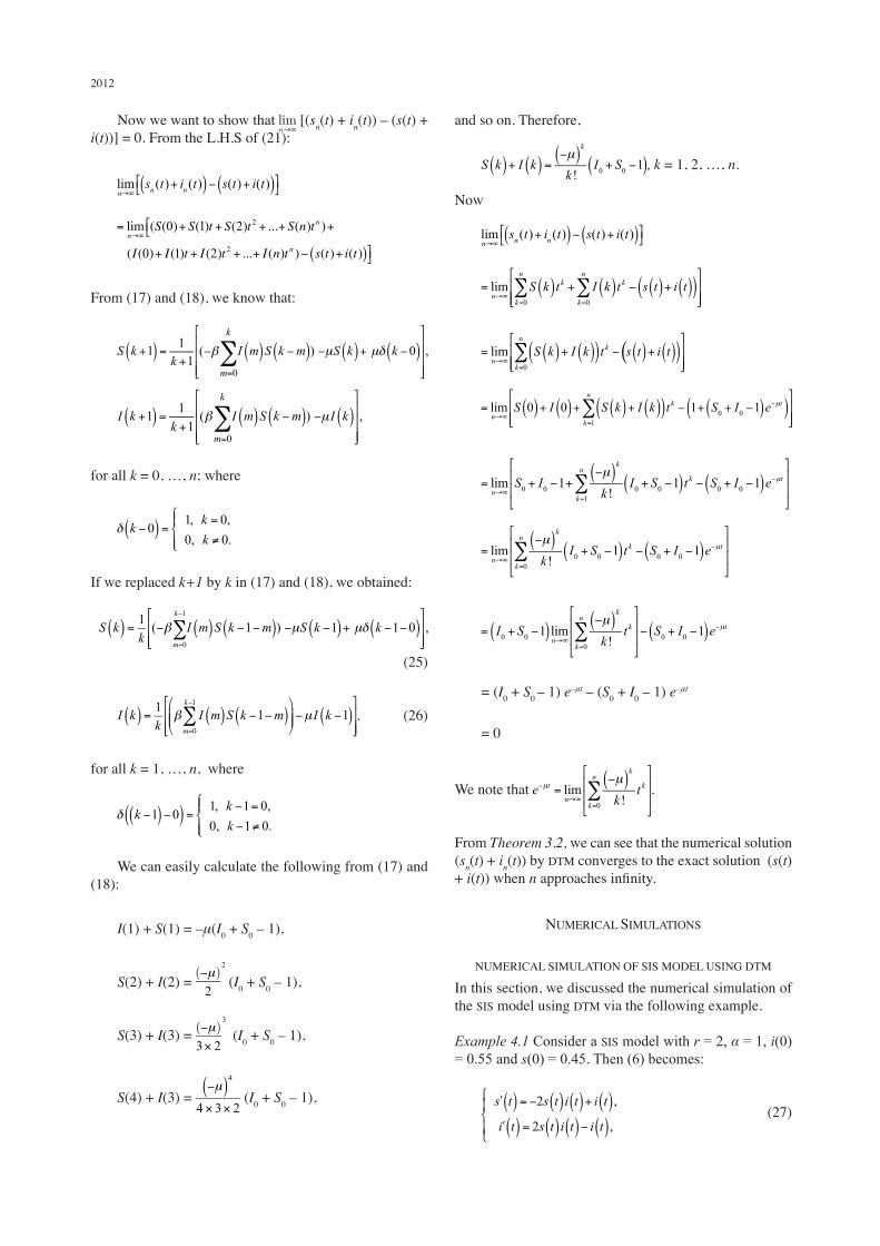
2012

Now we want to show that [(sn(t) + in(t)) – (s(t) + i(t))] = 0. From the L.H.S of (21):

From (17) and (18), we know that:

for all k = 0, …, n; where

If we replaced k+1 by k in (17) and (18), we obtained:

(25)

. (26)

for all k = 1, …, n, where

We can easily calculate the following from (17) and (18):

I(1) + S(1) = –μ(I0 + S0 – 1),

S(2) + I(2) = (I0 + S0 – 1),

S(3) + I(3) = (I0 + S0 – 1),

S(4) + I(3) = (I0 + S0 – 1),

and so on. Therefore,

, k = 1, 2, …, n.

Now

= (I0 + S0 – 1) e–μt – (S0 + I0 – 1) e–μt

= 0

We note that .

From Theorem 3.2, we can see that the numerical solution (sn(t) + in(t)) by DTM converges to the exact solution (s(t) + i(t)) when n approaches infinity.

NUMERICAL SIMULATIONS

NUMERICAL SIMULATION OF SIS MODEL USING DTM

In this section, we discussed the numerical simulation of the SIS model using DTM via the following example.

Example 4.1 Consider a SIS model with r = 2, α = 1, i(0) = 0.55 and s(0) = 0.45. Then (6) becomes:

(27)

2013

subject to the initial conditions:

i(0) = 0.55, s(0) = 0.45. (28)

Solution By applying the differential transformation method to (27), the following recurrence relations can be obtained:

(29)

(30)

I(0) = 0.55, S(0) = 0.45. (31)

In this example, we consider k from 0 to 11, and the results are listed in Tables 2 and 3. The accuracy of the solutions is illustrated in Figures 1 and 2.

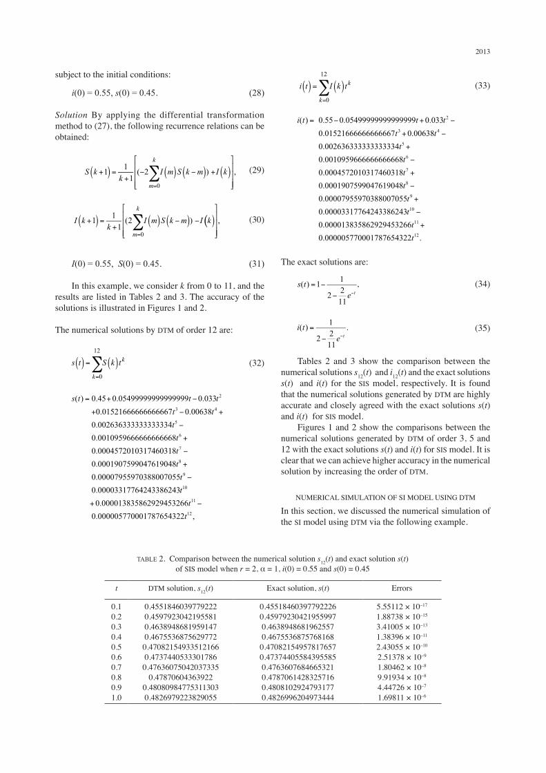
The numerical solutions by DTM of order 12 are:

(32)

(33)

The exact solutions are:

, (34)

(35)

Tables 2 and 3 show the comparison between the numerical solutions s12(t) and i12(t) and the exact solutions s(t) and i(t) for the SIS model, respectively. It is found that the numerical solutions generated by DTM are highly accurate and closely agreed with the exact solutions s(t) and i(t) for SIS model. Figures 1 and 2 show the comparisons between the numerical solutions generated by DTM of order 3, 5 and 12 with the exact solutions s(t) and i(t) for SIS model. It is clear that we can achieve higher accuracy in the numerical solution by increasing the order of DTM.

NUMERICAL SIMULATION OF SI MODEL USING DTM

In this section, we discussed the numerical simulation of the SI model using DTM via the following example.

TABLE 2. Comparison between the numerical solution s12(t) and exact solution s(t) of SIS model when r = 2, α = 1, i(0) = 0.55 and s(0) = 0.45

ErrorsExact solution, s(t)DTM solution, s12(t)t

5.55112 × 10–17

1.88738 × 10–15

3.41005 × 10–13

1.38396 × 10–11

2.43055 × 10–10

2.51378 × 10–9

1.80462 × 10–8

9.91934 × 10–8

4.44726 × 10–7

1.69811 × 10–6

0.455184603977922260.459792304219559970.46389486819625570.46755368757681680.470821549578176570.473744055843955850.47636076846653210.47870614283257160.48081029247931770.4826996204973444

0.45518460397792220.45979230421955810.46389486819591470.46755368756297720.470821549335121660.47374405333017860.47636075042037335

0.478706043639220.480809847753113030.4826979223829055

0.10.20.30.40.50.60.70.80.91.0

2014

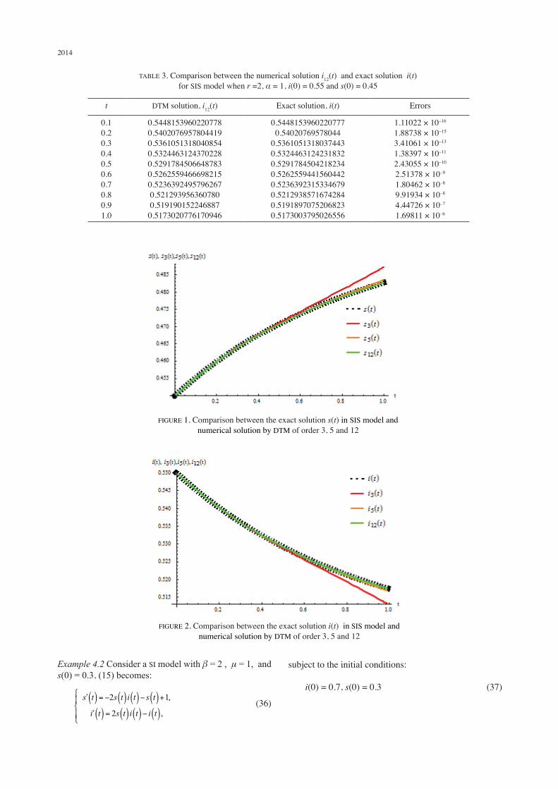
FIGURE 1. Comparison between the exact solution s(t) in SIS model and numerical solution by DTM of order 3, 5 and 12

FIGURE 2. Comparison between the exact solution i(t) in SIS model and numerical solution by DTM of order 3, 5 and 12

TABLE 3. Comparison between the numerical solution i12(t) and exact solution i(t) for SIS model when r =2, α = 1, i(0) = 0.55 and s(0) = 0.45

ErrorsExact solution, i(t)DTM solution, i12(t)t

1.11022 × 10–16

1.88738 × 10–15

3.41061 × 10–13

1.38397 × 10–11

2.43055 × 10–10

2.51378 × 10–9

1.80462 × 10–8

9.91934 × 10–8

4.44726 × 10–7

1.69811 × 10–6

0.54481539602207770.54020769578044

0.53610513180374430.53244631242318320.52917845042182340.52625594415604420.52363923153346790.52129385716742840.51918970752068230.5173003795026556

0.54481539602207780.54020769578044190.53610513180408540.53244631243702280.52917845066487830.52625594666982150.52363924957962670.5212939563607800.5191901522468870.5173020776170946

0.10.20.30.40.50.60.70.80.91.0

Example 4.2 Consider a SI model with β = 2 , μ = 1, and s(0) = 0.3, (15) becomes:

(36)

subject to the initial conditions:

i(0) = 0.7, s(0) = 0.3 (37)

2015

Solution By applying the differential transformation method to (36), the following recurrence relation can be obtained:

(38)

(39)

In this example, we consider k from 0 to 19 and the results are listed in Tables 4 and 5. The accuracy of the solutions is illustrated in Figures 3 and 4.

The numerical solutions by DTM of order 20 are:

(40)

(41)

The exact solutions are:

(42)

(43)

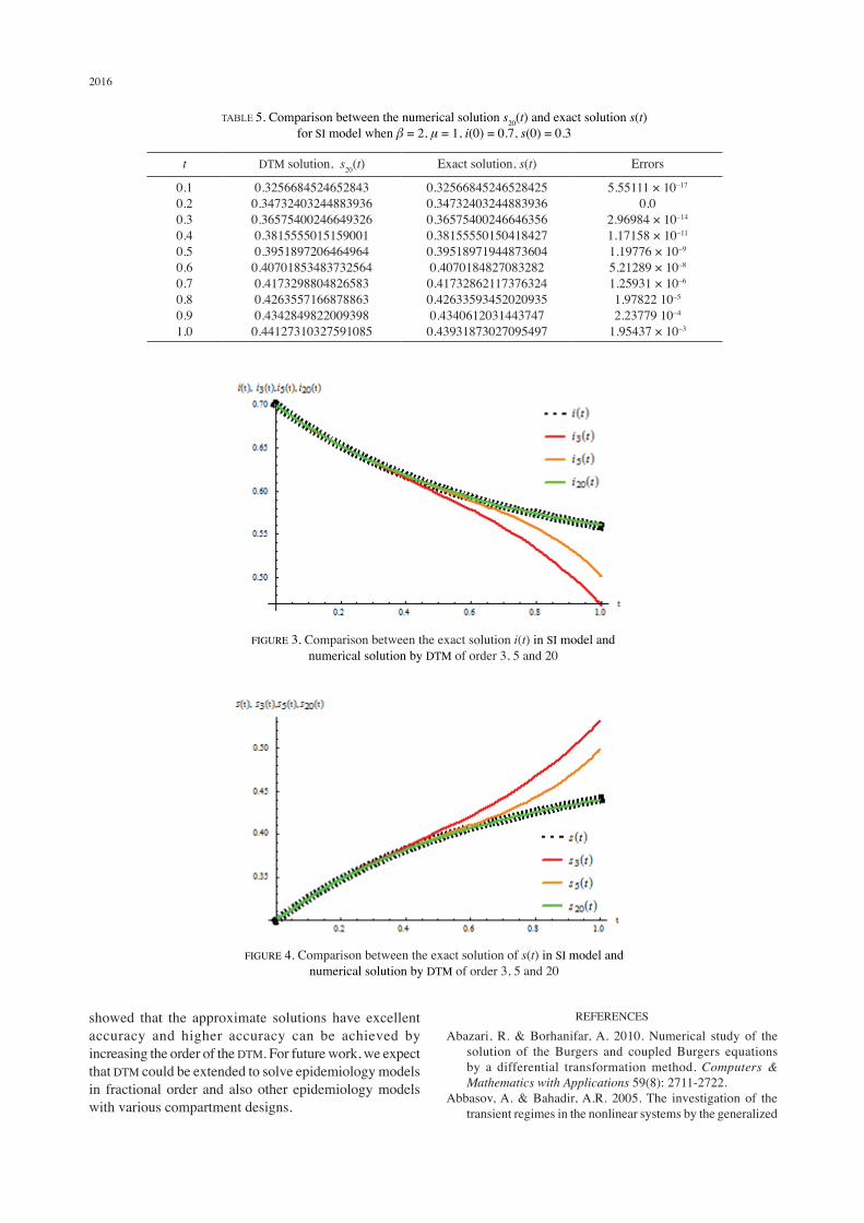
Figures 3 and 4 show the comparisons between the numerical solutions generated by DTM of order 3, 5 and 20 with the exact solutions s(t) and i(t) for SI model. It is clear that we can achieve higher accuracy in the numerical solution by increasing the order of DTM.

CONCLUSION

In this paper, we solved epidemic models of SIS without vital dynamics and SI with vital dynamics by the differential transformation method (DTM). Numerical experimentations

TABLE 4. Comparison between the numerical solution i20(t) and exact solution i(t) for SI model when β = 2, μ = 1, i(0) = 0.7 and s(0) = 0.3

ErrorsExact solution, i(t)DTM solution, i20(t)t

0.01.11022 × 10–16

2.97539 × 10–14

1.17157 × 10–11

1.19776 × 10–9

5.2129 × 10–81.25931 × 10–6

1.97822 × 10–5

2.23779 × 10–4

1.954373 × 10–3

0.67433154753471570.65267596755116060.63424599753350670.61844449848409990.60481027935350360.59298146516267440.58267011951734170.57364428331211370.56571501779906020.5587268967240892

0.67433154753471570.6526759675662220.63424599753350670.61844449848409990.60481027935350360.59298146516267440.58267011951734170.57364428331211370.56571501779906020.5587268967240892

0.10.20.30.40.50.60.70.80.91.0

2016

TABLE 5. Comparison between the numerical solution s20(t) and exact solution s(t) for SI model when β = 2, μ = 1, i(0) = 0.7, s(0) = 0.3

t DTM solution, s20(t) Exact solution, s(t) Errors

0.10.20.30.40.50.60.70.80.91.0

0.32566845246528430.347324032448839360.365754002466493260.38155550151590010.39518972064649640.407018534837325640.41732988048265830.42635571668788630.43428498220093980.44127310327591085

0.325668452465284250.347324032448839360.365754002466463560.381555501504184270.395189719448736040.40701848270832820.417328621173763240.426335934520209350.43406120314437470.43931873027095497

5.55111 × 10–17

0.02.96984 × 10–14

1.17158 × 10–11

1.19776 × 10–9

5.21289 × 10–8

1.25931 × 10–6

1.97822 10–5

2.23779 10–4

1.95437 × 10–3

FIGURE 3. Comparison between the exact solution i(t) in SI model and numerical solution by DTM of order 3, 5 and 20

FIGURE 4. Comparison between the exact solution of s(t) in SI model and numerical solution by DTM of order 3, 5 and 20

showed that the approximate solutions have excellent accuracy and higher accuracy can be achieved by increasing the order of the DTM. For future work, we expect that DTM could be extended to solve epidemiology models in fractional order and also other epidemiology models with various compartment designs.

REFERENCES

Abazari, R. & Borhanifar, A. 2010. Numerical study of the solution of the Burgers and coupled Burgers equations by a differential transformation method. Computers & Mathematics with Applications 59(8): 2711-2722.

Abbasov, A. & Bahadir, A.R. 2005. The investigation of the transient regimes in the nonlinear systems by the generalized

2017

classical method. Mathematical Problems in Engineering 2005(5): 503-519.

Abubakar, S., Akinwande, N.I., Jimoh, O.R., Oguntolu, F.A. & Ogwumu, O.D. 2013. Approximate solution of SIR infectious disease model using homotopy perturbation kethod (HPM). The Pacific Journal of Science & Technology 14(2): 163-169.

Akinboro, F.S., Alao, S. & Akinpelu, F.O. 2014. Numerical solution of SIR model using differential transformation method and variational iteration method. General Mathematics Notes 22(2): 82-92.

Alomari, A.K. 2011. New analytical solution for fractional chaotic dynamical systems using the differential transformation method. Computer and Mathematics with Applications 61(9): 2528-2534.

Arikoglu, A. & Ozkol, I. 2007. Solution of fractional differential equations by using differential transformation method. Chaos, Solitons & Fractals 34(5): 1473-1481.

Arikoglu, A. & Ozkol, I. 2006. Solution of difference equations by using differential transformation method. Applied Mathematics & Computation 174(2): 1216-1228.

Ayaz, A. 2004. Solutions of the systems of differential equations by differential transform method. Applied Mathematics & Computation 147(2): 547-567.

Batiha, K. & Batiha, B. 2011. A new algorithm for solving linear ordinary differential equations. World Applied Sciences Journal 15(12): 1774-1779.

Borhanifar, A. & Abazari, R. 2011. Exact solutions for non-linear Schrödinger equations by differential transformation method. Journal of Applied Mathematics & Computing 35(1): 37-51.

Chen, C.L. & Liu, Y.C. 1998. Solution of two point boundary value problems using the differential transformation method. Journal of Optimization Theory & Applications 99(1): 23-35.

Chen, C.K. & Ho, S.H. 1996. Application of differential transformation to eigenvalue problems. Applied Mathematics & Computation 79(2-3): 173-188.

Hassan, I.A.H. 2008. Application to differential transformation method for solving systems of differential equations. Applied Mathematical Modelling 32(12): 2552-2559.

Hassan, I.A.H. & Ertürk, V.S. 2007. Applying differential transformation method to the one-dimensional planar bratu problem. Contemporary Engineering Sciences 2(30): 1493-1504.

Jang, M.J. & Chen, C.L. 1997. Analysis of the response of a strongly nonlinear damped system using a differential transformation technique. Applied Mathematics & Computation 88(2-3): 137-151.

Jing, H. & Zhu, D. 2005. Global stability and periodicity on SIS epidemic models with backward bifurcation. Computers & Mathematics with Applications 50(8-9): 1271-1290.

Kermack, W.O. & McKendrick, A.G. 1927. A contribution to the mathematical theory of epidemics. In Proceedings of the Royal Society of London A: Mathematical, Physical & Engineering Sciences 115(772): 700-721.

Khan, H., Mohapatra, R.N., Vajravelu, K. & Liao, S.J. 2009. The explicit series solution of SIR and SIS epidemic models. Applied Mathematics & Computation 215(2): 653-669.

Korobeinikov, A. & Wake, G.C. 2002. Lyapunov functions and global stability for SIR, SIRS and SIS epidemiological models. Applied Mathematics Letter 15(8): 955-960.

Momani, S., Odibat, Z. & Hashim, I. 2008. Algorithms for nonlinear fractional partial differantial equations: A selection of numerical methods. Topological Method in Nonlinear Analysis 31: 211-226.

Nazari, D. & Shahmorad, S. 2010. Application of the fractional differential transform method to fractional order integro-differential equations with nonlocal boundary conditions. Journal of Computational & Applied Mathematics 234(3): 883-891.

Nucci, M.C. & Leach, P.G.L. 2004. An integrable SIS model. Journal of Mathematical Anaysis & Appication 290(2): 506-518.

Odibat, Z.M. 2008. Differential transformation method for solving Volterra integral equations with separable kernels. Mathematical & Computational Modelling 48(7-8): 1144-1149.

Pietro, G.C. 2007. How mathematical models have helped to improve understanding the epidemiology of infection. Early Human Development 83(3): 141-148.

Shabbir, G., Khan, H. & Sadiq, M.A. 2010. A note on exact solution of SIR and SIS epidemic models. arXiv preprint arXiv: 1012.5035.

Soltanalizadeh, B. & Branch, S. 2012. Application of differential transformation method for solving a fourth-order parabolic partial differential equations. International Journal of Pure & Applied Mathematics 78(3): 299-308.

Tari, A., Rahimi, M.Y., Shahmorad, S. & Talati, F. 2009. Solving a class of two-dimensional linear and nonlinear Volterra integral equations by the differential transform method. Journal of Computational & Applied Mathematics 228(1): 70-76.

Yicang, Z. & Liu, H. 2003. Stability of periodic solutions for an SIS model with pulse vaccination. Mathematical & Computational Modelling 38(3-4): 299-308.

Zhien, M., Liu, J. & Li, J. 2003. Stability analysis for differential infectivity epidemic models. Nonlinear Analysis: Real World Applications 4(5): 841-856.

Zhou, J.K. 1986. Differential transformation and its applications for electrical circuits. Huazhong University Press, Wuhan, China.

M.Z. Ahmad*, D. Alsarayreh & A. Alsarayreh Institute of Engineering Mathematics Universiti Malaysia Perlis, Pauh Putra Main Campus02600 Arau, Perlis Indera KayanganMalaysia

I. QarallehDepartment of MathematicsTafila Technical UniversityTafila 66110Jordan

*Corresponding author; email: mzaini.imk@gmail.com

Received: 23 May 2016Accepted: 13 February 2017