HAL Id: tel-01668439https://tel.archives-ouvertes.fr/tel-01668439

Submitted on 20 Dec 2017

HAL is a multi-disciplinary open accessarchive for the deposit and dissemination of sci-entific research documents, whether they are pub-lished or not. The documents may come fromteaching and research institutions in France orabroad, or from public or private research centers.

L’archive ouverte pluridisciplinaire HAL, estdestinée au dépôt et à la diffusion de documentsscientifiques de niveau recherche, publiés ou non,émanant des établissements d’enseignement et derecherche français ou étrangers, des laboratoirespublics ou privés.

Development of time-dependent characterisation factorsfor life cycle impact assessment of road traffic noise on

human health.Rodolphe Meyer

To cite this version:Rodolphe Meyer. Development of time-dependent characterisation factors for life cycle impact as-sessment of road traffic noise on human health.. Human health and pathology. Université de CergyPontoise, 2017. English. �NNT : 2017CERG0879�. �tel-01668439�

Université de Cergy-Pontoise

École doctorale sciences et ingénierie

Thèse

Development of time-dependent characterisation

factors for life cycle impact assessment of road traffic

noise on human health

Présentée par Rodolphe Meyer

Pour obtenir le grade de Docteur de l’Université de Cergy-Pontoise en sciences et technologies de l'information et de la communication

Spécialité : Sciences de l'environnement

Soutenue le 10 novembre 2017

Membres du jury :

Catherine Lavandier, Directeur de thèse

Rosario Vidal, Rapporteur

Manuele Margni, Rapporteur

Enrico Benetto, Examinateur

Dick Botteldooren, Examinateur

Maarten Messagie, Examinateur

Benoit Gauvreau, Examinateur

Frédéric Mauny, Examinateur et président du jury

Bruno Vincent, Invité

i

“Soon silence will have passed into legend. Man has turned his back on silence. Day after day he invents machines and devices that increase noise and distract humanity from the essence of life, contemplation,

meditation...tooting, howling, screeching, booming, crashing, whistling, grinding, and trilling bolster his ego. His anxiety subsides. His inhuman void spreads monstrously like a gray vegetation.”

― Jean Arp

Even if my PhD thesis only addresses environmental noise impact on human health, I want to put it in a wider context, the context of our era, our epoch: the Anthropocene. This term is not yet officially accepted by the geological community as a geological period. However, to anybody acknowledging the state of our common spaceship Earth, this word has a clear meaning. It is the epoch where the consequences of human activities are visible everywhere. Human activities have halved the world’s animal population. The climate, and thus the physical condition of life on our planet, is changing at an unprecedented speed. Oceans are acidifying to the point of putting in danger the life it contains, especially the unique coral reef ecosystems. New minerals are created and major substance cycles, such as nitrogen and phosphorus, are visibly modified. Wherever we look, the impacts of human activities dominate natural variations. The lights of the city replace the fireflies. Concrete spreads over the fields of past generations covering productive soils and pushing agricultural activities further away, leaving less and less space for wildlife. Noise is not an exception in the great picture of the Anthropocene. Soundscape ecologists have found human noise everywhere; anthropophony is taking over biophony and geophony. Chain saws and car alarms are more and more common in the songs of the lyrebirds.

The environmental conditions are changing for the worse. We are not only damaging ecosystems, but we are also damaging the ability of our planet to support our species. The Anthropocene is the epoch where a single species is crossing the planetary boundaries. In a few decades, humanity has passed from a world where the limits were so far that they were imperceptible to a world where the limits are so close that they define the possible space, narrower every day, in which our societies can move if they want to keep what is perceived as civilized state. The Anthropocene is about a world with physical limits, and for humanity, it is something new.

Despite scientific facts, neither societies, nor populations, nor economic thinking has yet to successfully grasp the multiple implications of this drastic change of perspective. Modern societies rely heavily on non-renewable resources and produce more pollution than the environment is able to absorb. For a large part, today’s thinkers are still using old models to think about the future or are taking refuge in the faith of an hypothetic technologic rescue. If scientists and facts are not able to weigh in the way we think and build the future, my generation will quickly face the unthought of, or worse, the unthinkable. The last generations, despite the efforts of many, did not drastically change the way humanity considers itself and its environment. We will not have the same luxury. The decades to come may be the most important in the evolutionary process of our civilization.

ii

Table of Contents 1 Introduction .................................................................................................................................................... 3

1.1 Life cycle assessment (LCA) ................................................................................................................ 3

1.2 Environmental noise.............................................................................................................................. 5

1.3 Main research questions ........................................................................................................................ 6

1.4 Structure of this PhD thesis ................................................................................................................... 6

2 Acoustical knowledge allowing integration in LCA....................................................................................... 8

2.1 DALY ................................................................................................................................................... 8

2.2 General consideration about noise and noise indicators ........................................................................ 9

2.3 Health impairments ............................................................................................................................. 11

2.3.1 Noise annoyance ............................................................................................................................. 11

2.3.2 Sleep disturbance ............................................................................................................................ 12

2.3.3 Cardiovascular disease .................................................................................................................... 12

2.3.4 Cognitive impairment in children ................................................................................................... 13

2.3.5 Tinnitus ........................................................................................................................................... 13

2.4 Conclusion .......................................................................................................................................... 13

3 Existing methods to include noise in LCA ................................................................................................... 15

3.1 Overview of the literature ................................................................................................................... 15

3.2 Methods ............................................................................................................................................... 16

3.3 Results ................................................................................................................................................. 16

4 Noise prediction model ................................................................................................................................. 18

4.1 Required data ...................................................................................................................................... 18

4.2 From noise emission to population exposure ...................................................................................... 18

4.2.1 Noise emission model ..................................................................................................................... 19

4.2.2 Noise propagation model ................................................................................................................ 20

4.2.3 Population exposure ........................................................................................................................ 21

4.3 Maximum search radius ...................................................................................................................... 22

4.3.1 Introduction..................................................................................................................................... 22

4.3.2 Methods .......................................................................................................................................... 23

4.3.3 Results ............................................................................................................................................ 23

4.4 Conclusion .......................................................................................................................................... 24

iii

5 Proposed method to develop CFs for environmental noise impact on human health ................................... 26

5.1 Selecting midpoints for this impact category. ..................................................................................... 26

5.2 Calculating a set of CFs for LCIA ...................................................................................................... 27

5.2.1 Inventory ......................................................................................................................................... 27

5.2.2 The development of CFs ................................................................................................................. 29

5.2.3 Health impairment and time periods ............................................................................................... 31

5.2.4 Geographical area ........................................................................................................................... 33

5.2.5 Practical considerations for the marginal approach ........................................................................ 37

5.3 Conclusion .......................................................................................................................................... 38

6 Results .......................................................................................................................................................... 40

6.1 Number of experiments and IRIS choice ............................................................................................ 40

6.2 Spatial variability of the raw results .................................................................................................... 43

6.2.1 Qualitative approach of the spatial variability of CFs for annoyance ............................................. 43

6.2.2 Understanding the key variables behind the spatial variability of CFmgn,HAP,LV,J ............................ 46

6.2.3 How to take into account the spatial variability .............................................................................. 51

6.2.4 Spatial variability of CFmgn,HAP,HGV,J ............................................................................................... 52

6.2.5 Spatial variability of the average CFs for annoyance. .................................................................... 53

6.2.6 Spatial variability of CFs for sleep disturbance .............................................................................. 56

6.2.7 Use of these surrogate models and generalisation .......................................................................... 58

6.2.8 Use of the uncertainty distributions and evaluation for the whole set of CFs. ................................ 58

6.3 Weighted mean of the CFs over the whole tested sample ................................................................... 61

6.3.1 Average approach ........................................................................................................................... 61

6.3.2 Marginal approach .......................................................................................................................... 63

6.3.3 Comparison between average and marginal approaches................................................................. 65

6.4 Influence of other sources of uncertainty ............................................................................................ 66

6.4.1 Influence of a systematic error on noise exposure levels ................................................................ 66

6.4.2 Influence of a random error on noise exposure levels .................................................................... 67

6.4.3 Influence of a higher error on lower noise exposure levels ............................................................ 67

6.4.4 Influence of an error on the noise emission level ........................................................................... 68

6.4.5 Sensitivity analysis ......................................................................................................................... 70

6.4.6 Influence of other sources of uncertainty for an average CF, CFavg,day,IRIS ...................................... 71

iv

6.5 Comparison to previous literature ....................................................................................................... 74

6.5.1 Environmental noise impacts on human health .............................................................................. 74

6.5.2 Distance-based CFs in the LCA literature ...................................................................................... 75

6.5.3 The specific case of Cucurachi ....................................................................................................... 77

6.6 Connecting to the inventory ................................................................................................................ 78

6.6.1 Reference vehicle used ................................................................................................................... 78

6.6.2 New elementary flows .................................................................................................................... 78

6.6.3 Calculating the output of the processes........................................................................................... 79

6.7 Practical use of the CFs ....................................................................................................................... 81

6.7.1 In existing road transportation processes ........................................................................................ 81

6.7.2 In the foreground ............................................................................................................................ 82

6.8 Conclusion .......................................................................................................................................... 84

7 Discussion ..................................................................................................................................................... 86

7.1 Applying this methodology to other noise sources ............................................................................. 86

7.2 Possible use of these factors outside road transportation .................................................................... 87

7.3 Limits .................................................................................................................................................. 87

7.3.1 Representativeness of the sample ................................................................................................... 87

7.3.2 Noise prediction model and dose-response relationships ............................................................... 90

7.3.3 Population location ......................................................................................................................... 91

7.3.4 Incomplete uncertainty quantification ............................................................................................ 92

7.4 Using the IRIS division of the territory as basis for the calculation .................................................... 92

7.5 Pertinence of spatialized CFs for the environmental noise question ................................................... 93

7.6 Distance-based approach and vehicle categories ................................................................................ 94

7.7 Use of marginal and average CFs ....................................................................................................... 95

7.8 Temporal differentiation of environmental noise impact on human health......................................... 96

7.9 Uncertainty of environmental noise impact ........................................................................................ 97

8 Conclusion and outlook ................................................................................................................................ 98

9 References .................................................................................................................................................. 100

10 Annex I .................................................................................................................................................. 105

11 Annex II ................................................................................................................................................. 120

v

Figures

Figure 1: Simplified cause-effect chain. _________________________________________________________ 29

Figure 2: Schematic representation of both marginal and average approaches. _________________________ 31

Figure 3: Health impairments considered and their link with noise indicators. __________________________ 31

Figure 4: Representation of the building point of view. _____________________________________________ 35

Figure 5: Representation of the road point of view. _______________________________________________ 36

Figure 6: The additional number of HAP for five different geographical areas __________________________ 38

Figure 7: Geographical areas considered. _______________________________________________________ 41

Figure 8: Schematic representation of the IRIS and the two buffers. __________________________________ 41

Figure 9: The 67 IRIS are represented in blue and their internal buffer in grey. __________________________ 42

Figure 10: Summary of the CFs notation. ________________________________________________________ 43

Figure 11: Weighted histograms of the CFs at midpoint level for annoyance. ___________________________ 44

Figure 12: Weighted histograms of the CFs at midpoint level for annoyance on a logarithmic scale. ________ 45

Figure 13: SM-based and NEPM-based CFmgn,HAP,LV,J________________________________________________ 48

Figure 14: CFmgn,HAP,LV,J plotted against the population density _______________________________________ 49

Figure 15: Geographical representation of the 67 IRIS and associated CFmgn,HAP,LV,J value. _________________ 50

Figure 16: Cumulative distribution function for the NEPM-based CFs and the fitted uncertainty distribution (line)

of CFmgn,HAP,LV,J. _____________________________________________________________________________ 52

Figure 17: SM-based and NEPM-based CFmgn,HAP,HGV,J with a linear (a) or logarithmic scale (b). _____________ 53

Figure 18: Cumulative distribution function for the NEPM-based and the fitted uncertainty distribution (line) of

CFmgn,HAP,HGV,J. ______________________________________________________________________________ 53

Figure 19: SM-based and NEPM-based CFavg,HAP,IRIS with a linear (a) or logarithmic scale (b). _______________ 54

Figure 20: SM-based and NEPM-based CFavg,HAP,extended with a linear (a) or logarithmic scale (b). ____________ 55

Figure 21: SM-based CFavg,HAP,IRIS obtained with (25) (a and b) and CFavg,HAP,extended obtained with (40) (c and d)

plotted against NEPM-based with a linear _______________________________________________________ 56

Figure 22: SM-based and NEPM-based CFmgn,HSDP,LV,J (a and b), CFmgn,HSDP,HGV,J (c and d) and CFavg,HSDP,extended (e

and f) ____________________________________________________________________________________ 57

Figure 23: Cumulative distribution function for the NEPM-based CFs and the fitted uncertainty distribution (line)

of CFmgn,HAP,extended. __________________________________________________________________________ 59

Figure 24: Influence of a systematic error on the noise exposure levels for the weighted mean of CFmgn,day,LV,J. 66

Figure 25: Influence of a systematic error on the sound emission levels for the weighted mean of CFmgn,day,LV,J. 69

Figure 26: Influence of a systematic error on both the sound emission level Lw and the noise exposure level Lden

for the weighted mean of CFmgn,day,LV,J. __________________________________________________________ 69

Figure 27: Influence of a systematic error on the noise exposure levels for the weighted mean of CFavg,day,IRIS. _ 72

Figure 28: Influence of a systematic error on both the sound emission level Lw and the noise exposure level Lden

for the weighted mean of CFavg,day,IRIS. __________________________________________________________ 73

Figure 29: Population exposure of major French cities _____________________________________________ 88

Figure 30: Density probability histogram of the population _________________________________________ 89

vi

Tables

Table 1: Disability weight and relative importance of the different types of health impairments _____________ 9

Table 2: DALY score and uncertainty for the two methods for one tire over one vkm. ____________________ 17

Table 3: Main characteristics of selected geographical areas. _______________________________________ 23

Table 4: Percentage of HAP, HSDP, and DALY explained by the change in the search radius. _______________ 23

Table 5: Ratio of the bounds of the 95-percentile confidence interval for all the CFs concerning the annoyance

midpoint indicator. _________________________________________________________________________ 46

Table 6: Weighted mean, minimum, maximum and parameters of the lognormal uncertainty distribution fitting

for all of the average CFs calculated in the IRIS or extended area. ____________________________________ 59

Table 7: Weighted mean, minimum, maximum and parameters of the lognormal uncertainty distribution fitting

for all of the marginal energy-based CFs. ________________________________________________________ 60

Table 8: Weighted mean, minimum, maximum and parameters of the lognormal uncertainty distribution fitting

for all of the marginal distance-based CFs. ______________________________________________________ 61

Table 9: Weighted mean of CFavg,HAP, CFavg,HSDP, CFavg,day and CFavg,night _________________________________ 62

Table 10: Distance-based and energy-based CFmgn at midpoint and endpoint levels for LVs, HGVs and

unspecified. _______________________________________________________________________________ 64

Table 11: Mean number of joules per vkm calculated from the weighted mean of the marginal CFs. ________ 65

Table 12: Comparing average and marginal CFs at the midpoint and endpoint level. _____________________ 65

Table 13: First order and total-effect Sobol indices of the considered uncertainties. ______________________ 70

Table 14: First order and total-effect Sobol indices of the considered uncertainties. ______________________ 74

Table 15: Comparison of the results of Müller-Wenk (2002) and the present work. ______________________ 75

Table 16: CFs calculated with the approach proposed by Cucurachi and CFs ____________________________ 78

Table 17: New elementary flows for distance-based CFs. ___________________________________________ 79

Table 18: Mean speed in km/h of LVs and HGVs for the weighted mean of marginal CFs. _________________ 81

Table 19: Human health impacts for one vkm. ___________________________________________________ 81

Table 20: Uncertainty distributions for the different parameters _____________________________________ 83

Table 21: Results of the uncertainty analysis. ____________________________________________________ 84

Table 22: Total-effect Sobol index for the five most important variables. ______________________________ 84

vii

Recurring acronyms

CF

DALY*

DW

EF

GIS

HAP*

HGV

HSDP*

IRIS

LCA

LCI

LCIA

LV

NEPM

pkm

SM

tkm

vkm

WHO

Characterisation factor

Disability-adjusted life year

Disability weight

Elementary flow

Geographical information system

Highly annoyed person

Heavy goods vehicle

Highly sleep disturbed person

Ilots Regroupés pour l'Information Statistique (Aggregated Units for Statistical Information)

Life cycle assessment

Life cycle inventory

Life cycle impact assessment

Light vehicle

Noise emission and propagation models

Passenger-kilometre

Surrogate model

Tonne-kilometre

Vehicle-kilometre

World Health Organization

*DALY, HAP and HSDP are acronyms. However, they are also used in this work as units for convenience and consistency. Therefore, it has been chosen not to agree these nouns in number as if they were unit symbols.

viii

Publications

Articles

Meyer, R., Benetto, E., Igos, E., Lavandier, C., 2016. Analysis of the different techniques to include noise damage

in life cycle assessment. A case study for car tires. Int. J. Life Cycle Assess. 1–14.

Meyer, R., Lavandier, C., Gauvreau, B., Benetto, E., 2017. Influence of the search radius in a noise prediction

software on population exposure and human health impact assessments. Appl. Acoust. 127, 63–73.

Oral presentations

Meyer, R., Igos, E., Benetto, E., 2016. Analysis of the different technique to include noise damage in life cycle

assessment. A case study for car tires. Presented at the SETAC Europe 26th Annual Meeting, Nantes, France.

Meyer, R., Lavandier, C., Gauvreau, B., Vincent, B., 2016. Intégration du bruit de trafic routier dans l’analyse du

cycle de vie: influence de la distance de propagation entre sources et habitations sur l’évaluation des populations

exposées, in: CFA 2016, Congrès Français D’acoustique. Université du Maine, le Mans, p. pp–2077.

Posters

Meyer, R., Benetto, E., 2015. Towards a new midpoint indicator for including noise impacts from mobility in

LCA. Presented at the 9th International Conference on Society & Materials (SAM9), Luxembourg.

Meyer, R., Benetto, E., Lavandier, C., 2016. Towards a new midpoint indicator for including noise impacts from

mobility in life cycle assessment. Presented at the SETAC Europe 26th Annual Meeting, Nantes, France.

Meyer, R., Benetto, E., Lavandier, C., 2017. A new method to integrate noise impact from road mobility in life

cycle assessment - preliminary results. Presented at the SETAC Europe 27th Annual Meeting, Brussels, Belgium.

MT180

I have participated to MT180, the French adaptation of Three Minute Thesis (3MT®), a competition where PhD

students have to effectively explain their research in three minutes. My presentation occurred on 25 th May 2017

and I won the public price. Video is available at https://www.youtube.com/watch?v=JKYUAKQ_k_g (first three

minutes).

Videos

Even if it is not directly linked to my PhD thesis, I have realised multiple videos on a Youtube channel Le

Réveilleur. The main discussed topic is environment (climate change, pollution, resource depletion…). In two

years, I have realised more than thirty videos and reached 10k subscribers. I consider that scientific dissemination

is a vital part of my job as a researcher in the environmental field since research in the environmental field has,

by nature, political implications. https://www.youtube.com/c/LeR%C3%A9veilleur.

ix

Abstract

Noise affects human health, causing annoyance, sleep disturbance and increasing the risk of cardiovascular

disease. The quantification of noise impacts highlights it as a public health problem for which road traffic is

mainly responsible. Life cycle assessment (LCA) is a technique to assess the environmental impacts of a product,

a service or a process. Despite taking into account many environmental problems, the impact of noise on human

health is not yet properly taken into account in LCA. The aim of this PhD thesis is to integrate the impact of traffic

noise on human health in the LCA framework.

The scientific elements of acoustics and epidemiology that allow this integration are presented. An analysis of the

existing methods is conducted by applying them to a case study. This helps to understand the advantages and

drawbacks of the different approaches while comparing the results they provide. A method to integrate the impact

of road traffic noise on human health in the LCA framework is then proposed. The method is based on noise

prediction software and data made available by the Directive 2002/49/EC. This makes it possible to establish,

with great precision, characterisation factors (CFs) connecting elementary flows of the LCA inventory with an

impact on human health.

The method is then applied to a sample of small geographic areas selected in the region surrounding the city of

Lyon (France). The application of the method and the analysis of the results provides a multitude of information

regarding the potential existence of a typology for spatial differentiation, the best form for the collection of noise

information at the LCA inventory level, the spatial variability of the CFs and the uncertainties that may be

associated with them. The CFs obtained show that integrating the impact of noise into LCA could double the

impact of road transport on human health. This PhD thesis also identifies further potential research topics. Similar

work needs to be done for other transport modes (mainly trains and airplanes) to allow for a fair comparison of

different transport modes in LCA studies. Repeating this method in other geographical areas with other acoustic

emission and propagation models and/or other noise prediction software would also help the generalisation of this

work and the assessment of possible sources of uncertainties.

x

Résumé court

Le bruit affecte la santé humaine, provoquant de la gêne, des troubles du sommeil et augmentant le risque de crise

cardiaque. Les quantifications de l’impact du bruit montrent que c’est un problème de santé publique et que le

trafic routier en est majoritairement responsable. L’analyse du cycle de vie (ACV) est une méthode d’évaluation

globale des impacts environnementaux d’un produit, d’un service ou d’un processus. Malgré la prise en compte

de nombreux problèmes environnementaux, l’impact du bruit sur la santé humaine n’est pas encore correctement

pris en compte dans l’ACV. L’objet de ce doctorat est d’intégrer dans l’ACV l’impact du bruit du trafic routier

sur la santé humaine.

Les différents éléments d’acoustique et d’épidémiologie qui permettent cette intégration sont présentés. Une

analyse des méthodes existantes est conduite en les appliquant à un cas d’étude. Cela permet de comprendre les

avantages et inconvénients des différentes approches tout en comparant les résultats qu’elles fournissent. Une

méthode pour intégrer l’impact du bruit du trafic routier sur la santé humaine dans l’ACV est ensuite proposée.

Cette méthode repose sur les logiciels de prédiction acoustique et les données rendues disponibles par la directive

2002/49/CE. Elle permet d’établir, avec une grande précision, des facteurs de caractérisations (CFs) reliant des

flux élémentaires de l’inventaire ACV à un impact sur la santé humaine.

La méthode est ensuite appliquée sur un échantillon de petites zones géographiques sélectionnées dans la région

lyonnaise. L’application de la méthode et l’analyse des résultats apportent de nombreux enseignements sur

l’existence potentielle d’une typologie pour la différentiation géographique, la meilleure forme pour la collecte

d’information sur le bruit au niveau de l’inventaire ACV, la variabilité spatiale des CFs ou encore l’incertitude

qui peut leur être associée. Les CFs obtenus montrent que l’intégration de l’impact du bruit en ACV pourrait

doubler l’impact du transport routier sur la santé humaine. Ce doctorat identifie également des pistes de recherche.

Des travaux similaires doivent être menés pour les autres moyens de transport (principalement trains et avions)

pour permettre une comparaison équitable des études ACV les impliquant. Répéter la méthode dans d’autres zones

géographiques, avec d’autres modèles d’émission et de propagation acoustique et/ou d’autres logiciels de

propagation acoustique apporterait également des éléments intéressants.

xi

Résumé long

Le bruit affecte la santé humaine, provoquant de la gêne, des troubles du sommeil et augmentant le risque de

risque cardiaque. Les quantifications de ce phénomène montrent qu’une large partie de la population est touchée

et l’Organisation Mondiale de la Santé (OMS) considère le bruit environnemental comme un problème de santé

publique. Lorsque l’on compare les différentes sources de bruit, on se rend compte que le trafic routier est

responsable de la majeure partie des impacts sur la santé humaine.

L’analyse du cycle de vie (ACV) est une technique d’évaluation globale des impacts environnementaux d’un

produit, d’un service ou d’un processus. Cette évaluation se fait sur l’ensemble du cycle de vie d’un produit, de

l’extraction des matières premières à la fin de vie. Malgré la prise en compte de nombreux problèmes

environnementaux, l’impact du bruit sur la santé humaine n’est pas encore correctement pris en compte par

l’ACV. L’objet de ce doctorat est de permettre l’intégration dans l’ACV de l’impact du bruit du trafic routier sur

la santé humaine.

Les différents éléments d’acoustique et d’épidémiologie qui permettent cette intégration sont d’abord présentés.

Une analyse des méthodes existantes pour intégrer le bruit dans l’ACV est conduite en les appliquant à un cas

d’étude. Cela permet de comprendre les avantages et inconvénients des différentes approches tout en comparant

les résultats qu’elles fournissent. Une méthode pour intégrer l’impact du bruit du trafic routier sur la santé humaine

dans l’ACV est ensuite proposée. Cette méthode repose sur les logiciels de prédiction acoustique et les données

rendues disponibles par la directive 2002/49/CE.

L’impact sur la santé humaine peut être calculé en termes de personnes fortement gênées et de personnes ayant

un sommeil très perturbé comme c’est traditionnellement le cas dans la majorité des études qui concernent

l’impact sanitaire du bruit environnemental. L’impact peut également être quantifié en DALY. Le DALY

(Disability Adjusted Life Years) est une unité de mesure communément utilisée par l’OMS et l’ACV pour

quantifier les impacts sur la santé humaine. Il permet d’agréger en une seule mesure des impacts sévères, allant

jusqu’à la mort prématurée d’un individu, avec des impacts bénins en utilisant un système de pondération. Cette

unité est donc très pratique pour comparer différents problèmes sanitaires entre eux. Cependant, la quantification

en DALY s’accompagne d’une plus grande incertitude que la quantification en termes de personnes fortement

gênées ou de personnes ayant un sommeil très perturbé. C’est pourquoi il est utile de garder tous ces indicateurs.

Les différents impacts environnementaux sont obtenus lors du calcul d’une ACV en multipliant les flux

élémentaires de l’inventaire par des facteurs de caractérisation (CFs). Un flux élémentaire est défini comme de la

matière ou de l’énergie entrant dans le système étudié provenant de l’environnement ou comme de la matière ou

de l’énergie libérée dans l’environnement par le système étudié. Il n’existe pas encore, dans la majorité des

inventaires du cycle de vie, de flux élémentaires permettant l’intégration de l’impact du bruit sur la santé humaine.

Une première possibilité est de se baser sur un flux élémentaire en véhicule-kilomètre (vkm) où un vkm est une

unité de mesure correspondant au mouvement d’un véhicule sur un kilomètre. La deuxième approche est

énergétique : au lieu de se concentrer sur la distance parcourue, on regarde l’énergie acoustique émise pendant ce

parcours (en joules).

xii

La méthode développée dans cette thèse repose sur l’utilisation du logiciel de prédiction acoustique CadnaA

(http://www.datakustik.com/en/products/cadnaa/) et des données spatiales et géographiques fournies par Acoucité

(http://www.acoucite.org/). Lesdites données couvrent la région du Grand Lyon (France) et contiennent des

informations sur la topographie, les bâtiments, la répartition de la population, la géométrie des routes et le trafic

routier. En utilisant ces données dans un logiciel de prédiction acoustique, il est possible de simuler

approximativement l’émission et la propagation du son et d’obtenir l’exposition de la population sur différentes

périodes de la journée : jour, soirée et nuit. Cette exposition au bruit sert de base au calcul des impacts du bruit

sur la santé.

La philosophie générale de la méthode proposée dans ce doctorat est de calculer l’impact du bruit du trafic routier

dans une zone clairement définie, puis d’augmenter le trafic et de refaire le même calcul. L’augmentation de

l’impact du bruit sur la santé est ensuite divisée par l’augmentation de trafic pour obtenir des CFs. Cette

augmentation de trafic est effectuée séparément pour les véhicules légers (LVs) et pour les véhicules lourds

(HGVs). Suivant le choix du flux élémentaire (en vkm ou en joule), la normalisation se fait avec l’augmentation

de trafic calculé en vkm ou en joule. L’impact sur la santé en termes de personnes fortement gênées est calculé à

partir d’un indicateur acoustique intégrant l’exposition au bruit sur les trois périodes : jour, soirée et nuit. L’impact

sur la santé en termes de personnes ayant un sommeil très perturbé est calculé sur l’exposition pendant la seule

période de nuit. Les CFs rendant compte de la gêne s’applique donc sur l’ensemble de la journée alors que les

CFs pour les troubles du sommeil ne s’appliquent que la nuit. Cela entraine une différentiation temporelle des CFs

en DALY mais uniquement sur deux périodes : jour & soirée et nuit. Les impacts sur la santé considérés ne

permettent pas de produire des CFs différenciés temporellement pour le jour et la soirée. Dans la suite du texte,

jour fait référence à jour & soirée puisqu’il n’est pas possible de les différencier.

Des CFs sont donc obtenus pour les LVs et les HGVs. Ils sont calculés en termes de personnes fortement gênées,

de personnes ayant un sommeil très perturbé ou de DALY. Les CFs en DALY sont calculés pour le jour, la nuit

et une période temporelle indifférenciée obtenue en faisant la moyenne pondérée des deux autres périodes. Enfin,

les CFS sont calculés en se basant sur un flux élémentaire en vkm ou en joule.

En supplément des CFs marginaux (dus à une augmentation marginale de trafic), des CFs moyens ont aussi été

calculés en divisant simplement l’impact sur la santé, sans aucune augmentation de trafic, par tout le trafic

responsable de cet impact. Pour pouvoir agréger ensemble les LVs et les HGVs, ces CFs moyens ne sont

calculables que par joule. En effet, agréger des LVs et des HGVs sur la base des vkm n’aurait pas de sens puisque

l’émission sonore par vkm de ces deux types de véhicule est très différente.

La méthode proposée est ensuite appliquée sur un échantillon de petites zones géographiques sélectionnées dans

la région lyonnaise (France). Un des buts de ce travail de thèse était d’identifier une éventuelle typologie. Les

zones géographiques ont été sélectionnées sur la base d’un découpage territorial existant, utilisé par l’INSEE, les

IRIS (îlots regroupés pour l’information statistique). Les IRIS sont construits pour être homogènes en termes de

démographie et de géographie. Utiliser ce découpage pour identifier les zones de calcul avait pour but de faciliter

l’identification d’une typologie.

xiii

À cause de la longueur des calculs, il n’a pas été possible de calculer les CFs sur l’ensemble des données fournies

par Acoucité. Un sous-échantillon d’IRIS a été sélectionné en les espaçant le plus possible pour couvrir les

situations géographiques et démographiques les plus différentes possibles. Au final, tous les CFs ont été calculés

dans 67 IRIS différents.

L’analyse des résultats a été très riche en information. Une première approche est d’observer la moyenne pondérée

des différents CFs sur les 67 IRIS dans lesquels les calculs ont été effectués, ladite pondération se faisant sur le

trafic présent dans l’IRIS. D’un point de vue statistique, un véhicule a beaucoup plus de chances d’être présent

dans un IRIS avec un fort trafic, il est donc important de faire une moyenne pondérée. L’analyse des moyennes

pondérées des CFs permet de voir que :

Les CFs calculés pour la nuit sont significativement plus élevés que ceux pour le jour. Cette différence vient

du plus fort impact sur la santé du bruit la nuit (puisqu’il affecte le sommeil) mais également du plus faible

trafic. Moins de trafic causant plus d’impact mène mécaniquement à des CFs plus élevés. La prise en compte

de cette différence peut-être compliquée dans la pratique actuelle de l’ACV puisque cela demande une

différentiation temporelle fine, en dessous de la journée. L’impact du bruit est donc un argument pour le

développement d’une différentiation temporelle fine dans le cadre de l’ACV.

Les CFs calculés par joule se montrent plus pratiques et plus fiables que les CFs calculés par vkm. Cela est

dû au fait que l’énergie acoustique dégagée par un vkm dépend de nombreux paramètres comme les

caractéristiques techniques du véhicule et de la chaussée, mais aussi de la vitesse du véhicule. Utiliser le vkm

entraîne donc une perte d’information par rapport à l’utilisation de l’énergie acoustique qui quantifie bien

plus précisément l’émission acoustique. L’approche par joule est donc préférée et permet un calcul des CFs,

probablement plus représentatif de la réalité. L’approche par joule facilite également la différentiation de

l’inventaire puisqu’il suffit d’ajouter à chaque procédé de transports routiers un flux élémentaire en joules

correspondant à l’émission sonore du véhicule concerné pour détailler très finement l’ensemble de

l’inventaire ACV.

Les CFs moyens ne sont que légèrement plus élevés que les CFs marginaux ce qui indiquerait une certaine

robustesse de la valeur des CFs par rapport à la situation dans laquelle ils ont été calculés. Ces CFs moyens

peuvent être utilisés dans un certain nombre de situation comme l’élaboration d’une empreinte bruit, similaire

aux différentes empreintes existantes comme l’empreinte carbone.

En comparant les CFs pour LVs et HGVs calculés par joule ou par vkm, on observe que les CFs pour HGVs

sont plus élevés par vkm mais deux fois plus faibles par joule. Considérant la différence d’émission sonore

entre un HGV et un LV, il est normal de trouver des CFs pour HGVs plus élevés par vkm. Mais, trouver des

CFs pour HGVs plus faibles par joule est une conséquence de la différence de répartition sur le réseau routier.

Les HGVs sont souvent plus concentrés sur les grands axes et moins présents dans les agglomérations. Un

joule d’HGV affecte donc moins la population. Cette différence va à l’encontre de ce qui est pratiqué dans la

littérature ACV où plusieurs méthodes considèrent que l’effet d’un HGV sur la santé humaine est 10 fois plus

xiv

important en se basant exclusivement sur la différence de puissance d’émission sans prendre en compte l’effet

de la différence de répartition.

L’analyse partielle de la sensibilité conduite pendant ce travail a montré une grande robustesse de la moyenne

pondérée des CFs marginaux par rapport à une potentielle erreur systématique sur la propagation, les CFs

moyens y étant plus sensible. Par contre, les CFs moyens et marginaux restent sensibles aux erreurs sur le

calcul de l’émission sonore puisque l’énergie acoustique dégagée par le trafic sert à normaliser l’impact qui

en résulte. Une analyse de la sensibilité des différents paramètres incertains montre la forte influence de

l’incertitude sur les facteurs utilisés pour convertir la gêne ou les troubles du sommeil en DALY.

En comparant les CFs trouvés dans ce travail avec des valeurs provenant de la littérature, on trouve que, dans

la majorité des cas les résultats, sont dans le même ordre de grandeur. Ce qui peut être surprenant quand on

considère la simplicité des premières approches et le peu de données disponibles alors.

En comparant ces CFs avec les autres catégories d’impact, on se rend compte que l’intégration de l’impact

du bruit pourrait doubler l’impact du transport routier sur la santé humaine tel que calculé par l’ACV. La

quantification de l’impact du bruit sur la santé humaine montre que cette catégorie d’impact n’est pas du tout

négligeable comparée à celles qui sont déjà bien intégrées dans l’ACV. Cela pourrait pousser à davantage de

travaux de recherche sur cette question.

Comme les CFs ont été calculés dans 67 zones géographiques différentes, on dispose de plus d’information que

la moyenne pondérée. On peut, en particulier, s’intéresser à la variabilité spatiale de ces CFs. Étudier cet aspect

permet également de tirer plusieurs enseignements :

L’analyse de la variabilité spatiale a permis de comprendre quelles étaient les principales variables expliquant

cette variabilité. La densité de population et la densité d’énergie sonore expliquent à elles seules une grande

partie de la variabilité spatiale observée sur nos 67 points. Il est même possible de proposer un modèle pour

chacun des CFs calculés en joules qui prédit les résultats avec une bonne précision. Ces modèles peuvent être

utilisés par un praticien connaissant bien la zone géographique dans lequel un transport a lieu pour calculer

des CFs personnalisés pour ladite zone.

Malgré la compréhension des principales variables à l’origine de la variabilité spatiale et le choix d’utiliser

un découpage en zones ayant des caractéristiques démographiques et géographiques homogènes (les IRIS),

il n’a pas été possible d’établir une typologie. De plus, la valeur des CFs peut évoluer très vite sur de courtes

distances. Or, la source du bruit dont on étudie l’impact est un véhicule routier. Cette source va se déplacer

sur une grande distance comparée à celle sur laquelle les CFs changent de valeur. Il paraît donc plus juste

d’utiliser une moyenne pondérée des CFs obtenues sur les 67 points, la pondération se faisant sur le trafic

contenu dans les différentes zones géographiques étudiées. La variabilité spatiale peut toujours être prise en

compte en proposant une distribution d’incertitude en plus de la moyenne pondérée. L’utilisateur de ces CFs

qui voudrait prendre en compte la variabilité trouvée dans nos résultats pourrait utiliser, par exemple, une

xv

analyse Monte-Carlo et les distributions d’incertitude fournies. Les résultats trouvés lors de ces travaux

rendent cette solution préférable à celle d’une typologie.

Cependant il est possible qu’une typologie existante n’ait pas été détectée et il serait intéressant de conduire des

expériences similaires en modifiant légèrement la méthode ou/et en l’appliquant ailleurs. Utiliser une grille

normalisée pour le découpage géographique peut être une meilleure approche comparée à l’utilisation des IRIS.

Ce choix initial affecte probablement peu le résultat. Mais, puisqu’il n’a pas été possible d’identifier une typologie

en utilisant les IRIS, il n’y a plus d’arguments pour supporter ce choix. La taille de la maille de la grille normalisée

est également une question importante. Le mieux serait d’utiliser une grille relativement petite (500m par

exemple) quitte à agréger ensemble plusieurs mailles si une typologie n’apparaît qu’à une plus large échelle.

Répéter cette approche dans d’autres zones géographiques pour voir si les mêmes résultats sont obtenus serait

également très intéressant. Cela permettrait d’avoir une meilleure idée de la variabilité qu’il peut exister entre

différentes villes et/ou différents pays. Quitte à répéter la méthode, il serait également intéressant de changer les

modèles d’émission, de propagation et/ou le logiciel utilisé pour voir si cela influe sur le résultat. L’utilisation de

logiciels libres pour la prédication acoustique serait également une grande avancée puisque cela permettrait un

meilleur contrôle des résultats et faciliterait la réplication par différents acteurs. Nous avons bon espoir que des

outils libres et efficaces soient développés dans les années à venir.

Appliquer cette méthode dans des zones à faible densité serait aussi un excellent complément aux travaux

développés ici qui concernent majoritairement du tissu urbain ou péri-urbain. Ces zones ne sont pas encore

beaucoup étudiées parce qu’elles ne sont pas concernées par la Directive 2002/49/CE. Il faudrait donc trouver ou

produire des données à leurs sujets avant de pouvoir les étudier. Il est difficile de prédire si les CFs calculés dans

des zones de faible densité seront différents de ceux trouvés ici.

Des travaux similaires doivent être menés pour les autres modes de transport, en particulier pour les trains et les

avions, pour permettre une comparaison équitable par les études ACV des différents modes de transports. Les

courbes de dose-réponse, reliant une exposition au bruit à un impact sur la santé, ne sont pas les mêmes pour tous

les modes de transport. De plus, pour traiter l’impact du bruit des avions et des trains qui vient généralement se

superposer au bruit routier, il faudra régler le problème de la multi-exposition.

1

Acknowledgements

First of all, my sincere gratitude goes to Prof. Catherine Lavandier and Dr. Enrico Benetto, who first believed in

me and gave me the opportunity to contribute to the world of international research. Their experience and solid

scientific knowledge has guided me through this new and challenging world. The joyful energy of Catherine

supported me throughout this work, while the expertise of Enrico oriented this work in the best direction. Both

have given me, at the same time, enough autonomy and assistance to let me express the best of myself.

I want to thank my steering committee, as these specialists from different horizons played an important role in the

success of my work. Benoit Gauvreau, a specialist of acoustic propagation, was always there to give significant

advice and support. Frédéric Mauny brought his expertise regarding the health impact of environmental noise.

Bruno Vincent provided high quality data. Integrating a new impact category in LCA should never be done

without the insight of specialists, and I am grateful to have found this insight in my steering committee.

I express my gratitude to Prof. Rosario Vidal and Prof. Manuele Margni, who generously agreed to review this

manuscript, and Prof Dick Botteldooren and Dr. Maarten Messagie who I was honoured to have as examiners.

With my supervisors and steering committee, they made sure that my defence was an enjoyable and memorable

moment with interesting discussions, comments and suggestions.

During my PhD, I started a Youtube channel, Le Réveilleur, mainly explaining environmental problems from the

scientific perspective. I consider this work of dissemination as part of my responsibility as a young researcher in

environment, even if I did it on my free time. I want to thank my community for the support and the many

encouraging messages. It has given me energy day after day during these three years. I also have to salute the

sincere involvement and the constructive criticisms of my dear friends Guillaume, Aurélien and Nicolas working

on the texts of each video and thus increasing the quality of the final product.

I want to thank Benoit and Paul, fellow PhD students. Benoit was working on characterization factors for

ecosystem services while I was working on mine on environmental noise. Even with different objects, we met

similar problems and our shared experience was very helpful. Paul worked on uncertainties and is passionate

about the philosophy of science. Since understanding uncertainty is always vital in a scientific project like mine,

his insight was useful too.

I am very thankful to Alya, who helped me so much by correcting this PhD thesis and the various articles I have

submitted. There is no point in producing knowledge if it cannot be transmitted. By improving the intelligibility

of my documents, you increased my usefulness as a researcher, and I cannot be thankful enough.

Sitting in an office all day long would have been more difficult without the laughter of Elorri, the anecdotes of

Mélanie, or the handsomeness of Thomas. Many thanks to all my colleagues for the interesting deep discussions,

the day-to-day jokes, and for being a good audience of mine. I have really appreciated the many discussions about

environment, economics, politics and the interactions in between that often occurred during coffee or lunch.

2

Finally, I want to thank Amandine. She went beyond providing me with help and support. She provided me a

small bubble where the importance of environmental problems were acknowledged as well as their implications

on our lives. In a society that seems determined to go straight to a global disaster, having someone who

understands your concerns and shares your view of the world helped a lot. Thank you for being that smart, rational

and supportive person by my side.

The research presented in this thesis was funded by the Luxembourg National Research Fund (FNR) under the

project DyPLCA (INTER/ANR/13/10/DyPLCA).

3

1 Introduction

Silent Spring (1962) is an environmental book written by marine biologist and conservationist Rachel Carson. It

played a major role in the creation of the United States Environmental Protection Agency (EPA) and is considered

by some as the starting point of the environmental movement (Hynes et al., 1989). It talks of the detrimental effect

of pesticides, especially dichlorodiphenyltrichloroethane (DDT), on the environment. The title is a reference to

the songbirds “silenced” by the extensive use of pesticides. Hearing plays a key role in the perception of threats

and opportunities in our direct environment, and it played a key role in the perception of one of the first major

environmental problems. Environmental problems have multiplied since the work of R. Carson, and both the

environmental movement and environmental science have considerably evolved and grown in importance. Among

the many developments of scientific knowledge in the environmental field, life cycle assessment could be an

effective tool to address the numerous environmental problems that modern societies are facing and help them to

become more and more sustainable.

1.1 Life cycle assessment (LCA)

LCA is a standardized technique to evaluate the potential environmental impacts generated by a product or a

system along its life cycle (ISO 14040, 2006; ISO 14044, 2006). Its standardization is one of the great strengths

of LCA, dividing it into four distinct phases. The first one, goal and scope, consists of defining the product or

service under study in the form of a functional unit, the system boundaries, and the assumptions and choices made

by the practitioner.

Once the object under study is clearly defined, the second step, life cycle inventory (LCI), consists in creating an

inventory of flows from and to nature according to the demand defined in the first step. The system under study

is separated in two parts: the foreground system and the background system. In the foreground system, the

processes are specifically modelled using primary data from the producer and secondary data from suppliers and

downstream users. The background is constituted by background processes usually representing the average

market consumption mix. These processes are not modelled by the practitioner. LCI is simply an accounting of

everything involved in the system under study: all the flows of materials, energy, emissions, etc. This inventory

is developed as a flow model of the technical system using data on inputs and outputs. Each of the processes in

this inventory is connected with other processes and/or elementary flows (EFs). EFs are specifically defined as

material or energy entering the system being studied that has been drawn from the environment without previous

human transformation, or as material or energy leaving the system being studied that is released into the

environment without subsequent human transformation (ISO 14040, 2006). Compiling an LCI can be a long and

complex task, and the quality of the data plays a crucial role in the accuracy of the results.

The results of the LCI provide a quantification of all inputs and outputs to and from the environment from all the

unit processes involved to respond to the functional unit under study in the form of EFs. This long list of substances

is difficult to interpret. This list of EFs still need to be converted into impacts, and this is done in the life cycle

impact assessment (LCIA) step. An impact category is a class representing an environmental issue of concern,

e.g. climate change, acidification, or ecotoxicity. For the impact categories already well-integrated in LCA, the

link between the LCI results and the impact takes the form of a characterisation factor (CF). A CF is a factor

4

derived from a characterisation model which is applied to convert an assigned life cycle inventory analysis result

to the common unit of the impact category indicator (ISO 14040, 2006). During the LCIA, each LCI EF is

multiplied by the relevant CFs to assess the impact of this EF per impact category. The result for a given impact

category is provided in (1), where s denotes the LCI EF, and CFs is the CF associated to this inventory flow

(Pennington et al., 2004).

= ∑ ∗ � (1)

Environmental impacts can be evaluated at a midpoint or endpoint level. A midpoint indicator can be defined as

a parameter in a cause-effect chain or network (environmental mechanism) for a particular impact category that

is between the inventory data and the category endpoint (Bare et al., 2000). For example, the effects on the

stratospheric ozone layer of all the stratospheric ozone depleting compounds accounted in a LCI will be grouped

in the midpoint impact category ozone depletion. The corresponding midpoint indicator is ozone depletion

potential (ODP) where the ODP of various substances is quantified based on the ozone depletion potential of 1 kg

of CFC-11, the reference substance.

Endpoint methods adhere to a damage-oriented approach and quantify environmental impacts on issues of

concern, such as ecosystem impacts, natural resources or human health. Endpoint method (or damage

approach)/model is a characterisation method/model that provides indicators at the level of Areas of Protection

(natural environment's ecosystems, human health, resource availability) or at a level close to the Areas of

Protection level (European Commission, 2011). An endpoint damage category such as human health will quantify

all the damage on human health by using CFs directly to the EFs of the LCI (1) or, more commonly, by multiplying

and aggregating the calculated midpoint categories (summing human health damage from climate change, ozone

depletion, etc.).

Several impact assessment methods proposing sets of CFs for multiple impact categories at midpoint and/or

endpoint levels already exist. Methodologies commonly used, include, among others: ReCiPe (Goedkoop et al.,

2009), Impact 2002+ (Jolliet et al., 2003) and ILCD handbook (European Commission, 2011). Some indicators

are assessed similarly between methodologies (for example, CFs for global warming potential), while others, such

as toxicity indicators, can be quite different between methodologies. Optionally, the results of the LCIA can be

normalized, grouped and weighted depending on the goal and scope of the LCA study.

The last step of an LCA, interpretation, draws conclusions and recommendations out of the study. Uncertainty

and sensitivity analyses should be conducted at this step to assess the reliability and identify possible issues.

Contribution analysis can also be conducted in order to determine which processes are most responsible for the

different environmental impacts.

Two different approaches can be identified in LCA: attributional and consequential. Definitions of these two

approaches can be slightly different between authors (Curran et al., 2005; Ekvall et al., 2016; European

Commission, 2011; Finnveden et al., 2009; Sonnemann et al., 2011). Attributional LCA aims at analysing an

object as it is in a static economy at a given time. Consequential LCA evaluates the consequences of a change in

a system under study. The difference between attributional and consequential concerns mainly the LCI. When

5

doing a consequential LCA, the practitioner has to include activities that are affected by the change under

consideration. An attributional LCA of an electric car will consider the life cycle impacts of its construction, use

phase and end-of-life in a given static background while a consequential LCA of a fleet of electric cars in a given

region over the next decade accounts for the change in infrastructures (charging stations, electricity production)

that it will entail.

One of the important advantages of LCA is to consider the whole lifecycle of the object under study and thus

avoid the displacement of pollution from one lifecycle step to another, e.g. from the use phase of a product to its

production phase. Having several impact categories is another big advantage of LCA because it allows to consider

trade-offs between different environmental problems, e.g. reducing climate change while increasing resource

depletion. LCA is a powerful technique because of its holistic approach. However, there is still room for

improvements in several directions, such as the quality of the databases, spatial and temporal differentiation of

both the inventory and the LCIA methods, the improvement of the uncertainties quantification, or the inclusion

of impact categories not yet taken into account. Among, these possible improvements, this thesis will focus on an

impact category not yet properly integrated into LCA: noise impact on human health.

1.2 Environmental noise

The disappearing joyful sound of songbirds was one of the first indicators of the impact of pesticides on the

ecosystem (Carson, 1962), and soundscape ecology continues to monitor ecosystems based on the sounds emitted

by vocalizing animals. But, sound coming from our environment is not the only precious indicator. During the

last decades, unwanted sounds, i.e. noise, has become an environmental problem of its own. Our remarkable

hearing system has played a major role in our survival as a permanently alert system, but it is now under the threat

of the many noises we have created: the anthropophony.

Sound is a physical vibration that propagates through a medium as an audible, mechanical wave of pressure and

displacement (Luxon and Prasher, 2007). The only medium considered in this thesis will be air, but sounds can

also propagate in other media, such as water, where it affects other species. A noise is a sound interpreted as loud,

unpleasing, annoying or unwanted. It is important to note that the difference between noise and sound only comes

from a difference in perception of this physical vibration. Most people will perceive a bird’s song in a positive

way while road traffic sound will be perceived negatively. That is why the first is not considered as noise while

the latter is. In this document, only anthropogenic sources are considered as noise. Environmental noise is thus

defined as the summary of outside noise pollution caused by transport and industrial and recreational activities.

Environmental noise is one of the most frequent sources of complaints among the European population, especially

in big cities or near major roads, railways and airports (Flash Eurobaromètre, 2010; Fritschi et al., 2011; Ifop,

2014). In the last decades, more and more attention has been given to the impact of environmental noise on human

health since the first inquiries (Abatement and Control, 1974; Health Council of the Netherlands, 1971).

Environmental noise is now considered as a public health problem (Fritschi et al., 2011), and the European

Commission has specifically addressed this environmental problem through the directive 2002/49/EC (Directive,

2002). Road transportation is responsible of the major part of the burden of disease from environmental noise

(Fritschi et al., 2011). Moreover, acoustic literature presents different dose-response relationships for different

6

transportation modes (Miedema and Oudshoorn, 2001). These elements, developed in the first section, justify the

focus of this thesis on noise from road transportation and its impact on human health.

To integrate the impact of environmental noise from road transportation in LCA, several questions have to be

successively answered.

1.3 Main research questions

This thesis attempts to answer four research questions.

Q1 Is there a sufficient amount of elements in the acoustic literature to allow for the integration of environmental

noise impacts from road transportation in life cycle assessment?

[Hypothesis 1] A causal-effect chain can be established between noise emissions from road transportation and

impacts on human health.

Q2 What are the advantages and drawbacks of existing methodologies to integrate noise impacts in life cycle

assessment?

[Hypothesis 2] In the day-to-day practice of LCA, impacts from environmental noise are not yet taken into

account. However, there are existing methods to integrate these impacts in LCA. These methods present both

benefits and drawbacks, and analysing and comparing them allow the proposal of a new approach.

Q3 How can noise emission and propagation models be used to integrate environmental noise impacts from road

transportation in life cycle assessment?

[Hypothesis 3] Noise prediction software using noise emission and propagation models with data collected at the

city scale allows the assessment of the noise exposure of a population. Moreover, parameters such as road traffic

can be changed in the noise prediction software allowing the assessment of not only the existing situation but also

the impact of changes. Using these tools to develop CFs that model the impact of environmental noise on human

health seems promising. Additionally, the data used to assess population exposure with noise prediction software

are more and more available at the European scale. It is possible to use these tools and data to develop CFs.

Q4 Can environmental noise CFs be derived in a practical format for their integration in LCA?

[Hypothesis 4] Analysing the application of the developed method could help to define the EFs used to take into

account noise emissions and the optimal midpoint(s) for noise impacts on human health. Applying the developed

method could help to know how to differentiate CFs temporally and spatially.

1.4 Structure of this PhD thesis

Section 2 includes a presentation of the DALY indicator, a measure of human health impacts created by the World

Health Organization and used in LCIA as an endpoint for the human health damage category. Then, sound

indicators that will be used throughout this work are introduced. Finally, a summary on the health impairments

involved in the human health impacts of environmental noise is proposed as well as the dose-response

relationships between sound indicators and these health impairments. This section answers Q1.

7

Section 3 presents existing methods to include environmental noise impacts on human health in LCA. This section

relies on my first paper published (Meyer et al., 2016) where existing methods have been applied to a case study

in order to identify the advantages, drawbacks and possible improvements of existing methods. The rationale,

methodology and main findings of the methods are quickly exposed. This section answers Q2.

Section 4 details the main tool used throughout this work: noise prediction software using sound emission and

propagation models. Noise prediction software allows one to estimate noise exposure of a population. This tool is

already used by the acoustic community to assess environmental noise and identify the population undergoing

critical noise level exposure. Noise prediction software is an important part of the innovative approach taken in

this work, and its operation is shortly described. Optimization of one parameter was the object of a second

publication (Meyer et al., 2017). Rationale, methodology and main findings of this paper are also described in this

section.

In section 5, the possible midpoints are discussed. Then, a general method to establish different sets of CFs on a

well-known geographical area is detailed. Some practical aspects of the application of this methodology are also

discussed. By proposing a method to develop CFs using noise prediction software, this section answers Q3.

Section 6 presents the results obtained with the above mentioned method and a deep analysis of these results. The

spatial variability of the different CFs is studied allowing the proposition of predictive models. Uncertainty is also

discussed, and the results are compared to the existing literature. The best solutions to produce EFs for these CFs

are presented and the CFs are applied to the case study presented in Meyer et al. (2016).

In Section 7, the utility, practicality and reliability of the different CFs proposed are discussed depending on the

situation in which they are used. The limits of the method proposed, the CFs developed and the tools used are also

discussed. The question of the temporal and spatial differentiation of CFs for environmental noise is examined

and recommendations are formulated for further work. Section 6 and 7 answer Q4.

In Section 8, the main findings are quickly summarised and further potential research topics are identified.

8

2 Acoustical knowledge allowing integration in LCA

Prior to any attempt to include environmental noise impact on human health as a new impact category of LCIA,

the relevant literature had to be analysed to identify the knowledge on which this integration is built. In this first

section, the elements allowing the integration of noise impacts in LCA will be reviewed.

There is a recent review paper presenting the state-the-art on the environmental noise impacts by the World Health

Organisation (WHO) (Fritschi et al., 2011). It shows sufficient evidence of the mechanistic links between

population exposure to environmental noise and five different health impairments: cardiovascular disease,

cognitive impairment in children, sleep disturbance, tinnitus, and annoyance. More importantly, the WHO was

able to quantify the human health impact of environmental noise. Like other burdens of disease, the results are

given in disability-adjusted life years (DALY), an indicator measuring damage on human health. DALY is also

used in LCA as an endpoint indicator for human health damage.

2.1 DALY

The human health damage HH calculated in DALY combines the years of life lost due to premature death (YLL)

and the years lived with disability (YLD) (Murray, 1994) as shown in (2).

[ ��] = ��� + �� (2)

In the health impairments considered by the WHO (Fritschi et al., 2011), cardiovascular disease is the only one

that can provoke death, so it will be the only one to account for in the YLL category. The cases of non-fatal

cardiovascular diseases will be accounted in YLD. The YLL is directly taken into account as shown in (3) where

N is the number of deaths due to the studied condition, and L is the difference between the anticipated life

expectancy and the age of premature death. Considering the cardiovascular diseases in terms of YLL requires

knowing the standard life expectancy and ages of death of the fatal cases of cardiovascular disease.

��� = ∗ � (3)

Non-fatal cases of cardiovascular disease, cognitive impairment in children, sleep disturbance, tinnitus and

annoyance and will be accounted as DALY in terms of YLD, as calculated in (4). I is the number of incident cases

for the studied condition, disability weight (DW) reflects the severity of the disability on a scale from zero (no

adverse health effects) to one (equivalent to death), and D is the average duration of the disability in years. DWs

are determined by health impairment and does not vary with age. DWs cannot be measured or objectively

elaborated. DWs are mostly assessed by panel of medical experts (Haagsma et al., 2014). They are uncertain and

can evolve over time.

�� = ∗ � ∗ (4)

To integrate the five types of health impairments considered here on a temporal period, Fritschi et al. (2011) used

a duration of one year. In other words, the exposure to environmental noise during one year will induce a health

impairment only during this period of study. The total HH from environmental noise is then given by (5).

9

[ ��] = ∑ ∗ � + ∑ ∗ � (5)

The disability weights and the relative importance of one health impairment among the sum is given in Table 1.

Table 1: Disability weight and relative importance of the different types of health impairments considered by Fritschi et al.

(2011).

Health impairment Disability weight

(DW)

Relative importance among the whole

burden of disease from environmental noise

Sleep disturbance 0.07 55.9%

Annoyance 0.02 36.3%

Cardiovascular disease 0.405 3.7%

Cognitive impairment in children 0.006 2.8%

Tinnitus 0.120 1.3%

Fritschi et al. (2011) found an overall burden of disease for environmental noise ranging between 1.0 and 1.6

million DALY over 285 million people living in agglomerations with more than 50,000 inhabitants in Western

Europe. This corresponds to an impact per person ranging between 0.0035 and 0.0056 DALY/year for the studied

population. Assuming a constant impact over a lifetime of 80 years, it leads to a loss of 3-5 months of healthy life.

This amount is quite important compared to other impact categories already present in LCA. For example, van

Zelm et al. (2008) considered human health effects of ozone and fine particulate (PM10) in Europe and found an

average 0.003 DALY/person/year (or 3 months of healthy life loss over a lifetime of 80 years assuming constant

emission rates). Franco et al. (2010) also found an environmental noise impact in the same order of magnitude as

that of air pollution for the case of road transportation. This validates another decision criterion for the

development of this new impact category in LCA (Cucurachi et al., 2014): the results of the quantification

highlight the importance of the burden from environmental noise compared to other human health impact

categories. Moreover, there are no reasons to think that transportation will become less important for our global

economy in a near future.

To include environmental noise in LCA, one condition is still unanswered. Are there mechanistic links between

environmental noise and human health impacts? To present potential links and decide of their possible use in the

framework of LCA, some acoustical indicators have to be shortly presented.

2.2 General consideration about noise and noise indicators

Sound is a physical vibration that propagates through a medium, e.g. air, as an audible, mechanical wave of

pressure and displacement. It can be measured in sound pressure level, Lp, as defined in (6), where log is the

decimal logarithm, p is the sound pressure in Pascal and p0 is the reference pressure (equal to 2*10-5 Pa) (ISO

3744, 2010). For this whole document, log will always refer to the decimal logarithm while ln will refer to natural

logarithm. The logarithmic scale used to measure sound takes into account the large scale and non-linear response

10

of the human sound pressure sensitivity. The reference pressure, p0, is considered as the smallest detectable sound

pressure by humans at 1 kHz.

� = ∗ log (6)

When assessing population exposure to environmental noise, the sound pressure level at a given time, LP, is less

interesting than the equivalent A-weighted sound pressure level, LAeq. A-weighting is a frequency correction

applied to sound levels in an effort to account for the relative loudness perceived by the human ear (“International

Standard IEC 61672-1,” 2003). A-weighting is thus commonly used to assess environmental noise (Luxon and

Prasher, 2007). LAeq considers a steady sound pressure level that has the same total energy as the actual noise over

a given period of time, T. In the calculation of LAeq in (7), pA is the instantaneous A-weighted sound pressure in

pascal (ISO 3744, 2010).

�� = ∗ log ∗ ∫ � ² (7)

Because noise level is not constant throughout the entire day, and because activities, location, and even the

susceptibility of humans are modulating the potential impact of environmental noise on health, a day has to be

separated into smaller and most homogeneous periods of time. In Europe, three time periods have been defined:

day, evening and night. These time periods cover the whole day and last for 12 h, 4 h and 8 h, respectively. The

limits for these different periods are given in the European Directive 2002/49/EC relative to the assessment and

management of environmental noise. The default values are from 7 a.m. to 7 p.m. for the day, from 7 a.m. to

11 p.m. for the evening, and from 11 p.m. to 7 a.m. for the night. However, it can change from one country to

another (Directive, 2002). For example, in France, the sound emission model (SETRA Copyright (Collective),

2009a) defines the day between 6 a.m. and 6 p.m., evening between 6 p.m. and 10 p.m., and night between 10 p.m.

and 6 a.m.. The periods have the same length but not the same limits. The resulting A-weighted equivalent noise

pressure levels integrated over day, evening, and night are Lday, Levening and Lnight.

A derived sound indicator for population exposure is Lden. It is the day-evening-night equivalent sound pressure

level, Lden, recommended by the European Directive 2002/49/EC to represent environmental noise. Lden is

calculated in (8) from the A-weighted equivalent sound pressure levels of the three defined periods.

� = ∗ log ∗ � �� + ∗ � � �+ + ∗ � ��ℎ�+

(8)

In the definition of Lden, penalties of +5 dB(A) for the evening period and +10 dB(A) for the night are added to

take into account the higher sensitivity of the exposed population over these periods of the day. For example,

environmental noise at night is more disruptive since people are sleeping (Luxon and Prasher, 2007).

For the emission part, roads are modelled by succession of acoustically homogeneous sections of line-sources

distributed over the road platform. A sound emission power per metre of line-source Lw/m is associated with each

acoustically-homogeneous section (SETRA Copyright (Collective), 2009a). Lw/m is linked to the sound power per

11

metre of line-source W/m by equation (9) where W0 is the reference sound power of 10-12 watts. Calculation of Lw/m

will be further detailed in 4.2.1.

� / = ∗ log (�/� ) (9)

Lw/m, Lday, Levening, Lnight and Lden will be used throughout this thesis. Now that these indicators have been accurately

defined, the links between environmental noise exposure and human health impact can be presented in a short

review of the health impairments identified by the WHO (Fritschi et al., 2011) and their relevance for integration

in LCA.

2.3 Health impairments

2.3.1 Noise annoyance

Noise annoyance is widely used as a basis for evaluating the impact of environmental noise on the exposed

population (Directive, 2002). Annoyance may provoke a large variety of negative responses (e.g. anger,

disappointment, dissatisfaction, depression, anxiety…) and is associated with psychological syndromes, like

tiredness and stress (Fritschi et al., 2011). Since health is defined by the WHO as a state of complete physical,

mental and social well-being and not merely the absence of disease or infirmity (Berglund et al., 1999), noise-

induced annoyance is considered as an adverse effect on health.

At individual level, the variation in noise annoyance can be explained by acoustical factors only for a third, by

non-acoustical factors for another third while the last third can be attributed to measurement errors, stochastic

variations or unknown factors (Guski and others, 1999). Non-acoustical factors include noise sensitivity, fear of

harm connected with the source, ability to cope with the limitation, concerns about property devaluation, etc.

(Fyhri and Klæboe, 2009; Guski and others, 1999; Kroesen et al., 2008). But at community level, there is a direct

link between noise exposure and the percentage of highly annoyed persons (HAP).

The exposure-response relationships used by Fritschi et al. (2011) to derive the percentage of HAP is detailed in

Miedema and Oudshoorn (2001) for aircraft (10), road traffic (11) and railways (12). These relationships are given

for Lden ranging between 45 and 75 dB(A). The exposure-response relationships proposed by Miedema and

Oudshoorn (2001) are based on the analysis of a large data set linking annoyance to the exterior noise exposure

level at the most exposed face of a dwelling. These exposure-response relationships do not explicitly take into

account sound insulation (for example) but instead consider it implicitly, since they link annoyance inside a

dwelling with the noise exposure levels outside of it

Aircraft: % = − . ∗ − ∗ � − − . ∗ − ∗ � − + .∗ � −

(10)

Road traffic: % = . ∗ − ∗ � − − . ∗ − ∗ � − + .∗ � −

(11)

12

Railways: % = . ∗ − ∗ � − − . ∗ − ∗ � − + .∗ � −

(12)

Also, two important elements have to be noted. First, there are different exposure-response relationships for the

different transport modes. For the same noise exposure level, a train does not have the same effect on sleep

disturbance as noise coming from road traffic. Noise cannot be simply aggregated in terms of energy over different

transport modes! Impact from different sources must be calculated separately since there are different exposure-

response. The case of multi-exposure is even more complex and is discussed in subsection 7.1. Second, annoyance

is calculated from the exposure in Lden, annoyance is a consequence of the exposure over the whole day and is

also affecting the concerned population during the whole day.

2.3.2 Sleep disturbance

Noise affects sleep directly (e.g. awakening, sleep stage changes…) and indirectly (e.g. daytime performance,

cognitive function deterioration), with both yielding long-term effects. Acute and chronic sleep restrictions or

fragmentations have a large number of effects on human health (e.g. memory consolidation, risk of accidents…).

Fritschi et al. (2011) advise an exposure-response relationship from epidemiological studies based on Miedema

et al. (2002) detailed in (13) for aircraft, in (14) for road traffic and in (15) for railways. These relationships can

be used to obtain the number of highly sleep disturbed persons (HSDP) by knowing the population’s exposure to

road transport at night. These relationships are given for Lnight ranges between 45 and 65 dB(A). The noise

exposure level Lnight is the exterior noise exposure level at the most exposed façade during the night period.

Aircraft: % = . ∗ � ℎ − . ∗ � ℎ + . (13)

Road traffic: % = . ∗ � ℎ − . ∗ � ℎ + . (14)

Railways: % = . ∗ � ℎ − . ∗ � ℎ + . (15)

Once again, the link between a given exposure and the resulting human health impact is dependent upon the source

of the noise. On the whole range of exposure where these relationships are valid, road transportation has less

impact than planes and more impact than trains. The quantification of sleep disturbance is calculated from Lnight,

meaning that this health impairment will only occur at night and is the consequence of transportation during the

night period.

2.3.3 Cardiovascular disease

Cardiovascular disease includes ischaemic heart disease, hypertension and stroke. Ischaemic heart disease is

responsible for 12.6% of deaths worldwide (Lopez and others, 2006). A review of existing epidemiological studies

suggests a higher risk of cardiovascular diseases in people chronically exposed to high levels of road traffic

(Fritschi et al., 2011). Main sources include Van Kempen et al. (2002), Babisch and others (2008) and Babisch et

al. (2009). And this question continues to be developed (Babisch et al., 2013; Hansell et al., 2013; Sørensen et al.,

2012)

13

Among the different diseases included in ischaemic heart disease, only myocardial infarction has been linked to

environmental noise. To calculate the burden of disease from myocardial infarction (heart attack), Fritschi et al.

(2011) used an odds ratio defined by the polynomial approximation given in (16), only valid for a value of the

daytime noise indicator Lday,16h between 55 and 80 dB(A), where Lday,16h is a metric aggregating sound power level

during day and evening periods without penalties. This odds ratio refers to the odds that a myocardial infarction

is likely to occur at a particular exposure compared to the odds of this outcome occurring in the absence of

environmental noise.

= . − . ∗ � , ℎ ² + . ∗ � , ℎ (16)

The odds ratio OR is used to calculate the attributable fraction for each exposure group, and the resulting

population-attributable fraction will give the proportion of cases of myocardial infarction due to noise exposure.

The population-attributable fraction is then multiplied by the number of fatal and non-fatal myocardial infarctions

within the studied zone. Applying this methodology attributes the number of fatal and non-fatal myocardial

infarctions due to noise exposure.

To apply this method, the exposure of the population and the number of cases of myocardial infarction have to be

known. Accessing the cases of myocardial infarction can be a serious limit since this type of information may not

be available or may be difficult to obtain for confidentiality reasons. And, even if this information is available, it

has to be known in the geographical area studied.

2.3.4 Cognitive impairment in children

Fritschi et al. (2011) also calculated the cognitive impairment in children at school induced by environmental

noise. Fritschi et al. (2011) underlined that this assessment is only supported by a small number of papers, and the

link between population exposure and health impairment seems less reliable than sleep disturbance and

annoyance, although this has been further investigated by Clark et al. (2013), Pujol et al. (2015), Levain et al.

(2015) and Stansfeld and Clark (2015) among others. However, this health impairment needs specific information

about the exposure of children. Such information is difficult to access and requires a specific and separate

modelling while the noise prediction method assumes each person is located at his place of residence. Even if all

the necessary information were available, a specific modelling should be done where the children would be located

in their respective schools and considered separately for this specific health impairment. Thus, cognitive

impairment in children will not be considered in the rest of this work.

2.3.5 Tinnitus

Tinnitus is also considered in (Fritschi et al., 2011), but it only comes from leisure noise (e.g. concerts, sport

events, firecrackers) and so it is out of the scope of this thesis. Tinnitus will be excluded from the rest of this work.

2.4 Conclusion

First of all, the different elements presented here highlight the need to integrate environmental noise impacts in

LCA because of the high burden of disease found by Fritschi et al. (2011). Moreover, there is a sufficient amount

of elements in the acoustic literature to allow for this integration.

14

Sleep disturbance and annoyance account for 92.2% of the burden of disease from environmental noise, a major

part of the overall environmental noise impact. As highlighted, different transportation modes (road, plane and

train) have different exposure-response relationships for annoyance and sleep disturbance and it is an important

aspects while considering the integration of environmental noise in LCA. Taking this into account, the sound

energy coming from these different sources cannot be simply summed up prior to calculating impacts on human

health. Different noise sources would lead to separate assessments or to advance models able to deal with multi-

exposure. Since 83% of the human health damage coming from annoyance and 89% of the human health damage

coming from sleep disturbance is caused by road transportation (Fritschi et al., 2011), it has been decided to focus

exclusively on road transportation. Potential extrapolation to other transportation modes and noise sources will be

discussed in 7.1 as well as the problem of multi-exposure.

The integration of environmental noise impacts on human health in the LCA framework has already been

discussed in the scientific community and there have been several attempts to do it. Since we have a clearer view

on how environmental noise impacts human health, it will be easier to understand the earlier attempts to include

it in LCA.

15

3 Existing methods to include noise in LCA

This section is based on Meyer et al. (2016). A summary is proposed here with the most interesting outcomes of

this article but, if preferred, the reader can refer to the full article in Annex I.

Given the preceding section, the effects of noise should be reflected in the assessment of products involving

significant transportation steps as well as of large scale systems, like regional mobility. Despite this need, the

integration of traffic noise damages on human health in LCA is still debated. Several attempts to include noise

impacts on human health in LCA have already been conducted, but none of these methods have allowed systematic

integration in LCIA. Noise impact is not yet included in the day-to-day practice of LCA.

The rationale behind Meyer et al. (2016) was to put in practice the existing methodologies to include noise in

LCA. Since extensive and recent reviews on the matter were already existing (Althaus et al., 2009; Cucurachi et

al., 2012), applying the different approaches on a case study was thought as an excellent way to understand and

address the problem of noise integration in LCA. Since the noise impact category is still in development, it was

important to understand the applicability and the outcomes given by the available methodologies. The objective

of Meyer et al. (2016) was threefold:

i) to evaluate the importance of noise damage as compared to other environmental contributions on human

health (in DALY);

ii) to analyse how the different methods for noise damage assessment are sensitive to different input noise

levels;

iii) to compare the results obtained from different methods.

3.1 Overview of the literature

The first operational method was developed by Müller-Wenk (2004, 2002, 1999) to evaluate the damage on human

health due to additional noise levels generated by cars and lorries using annoyance as midpoint indicator for the

noise impact category. This method was then adapted by Doka (2003) who used the SonRoad model (Heutschi et

al., 2004) for the determination of emission levels. Later, Althaus et al. (2009) included data from SonRoad and

from Steven (2005) to better distinguish different types of vehicles and situations. Nielsen and Laursen, (2005)

defined the noise nuisance impact potential in person*seconds, but unfortunately their model does not allow

repeatability because of the lack of necessary information. The last development of the method developed by

Müller-Wenk, (2002, 2004) was achieved by Franco et al. (2010). Finally, Cucurachi et al. (2012) and Cucurachi

and Heijungs (2014) proposed a set of CFs linking any type of noise (not only due to transportation) to a midpoint

indicator in person*Pa*s (number of people exposed to a certain sound pressure for a certain time duration).

Conversion factors to reach the human health damage endpoint are also proposed. The latter two approaches had

never been applied in a case study prior to Meyer et al. (2016).

Later in my work, I found that Moliner et al. (2014) pursued the work of Franco et al. (2010), without significant

changes to the global approaches. Also, Ongel and Sezgin (2016) developed a framework to assess the reduction

in terms of human health damage for several noise abatement measures (change in road surface, change in speed

16

limit). Ongel (2016) proposed CFs for nine municipalities of Istanbul in DALY.person-1.year-1.mW-1.m. These

last works were not discussed in Meyer et al. (2016).

In most LCA studies, noise impact is not yet taken into account, even when traffic is specifically modelled in the

foreground (Althaus et al., 2009). Two LCIA methodologies Frischknecht and Büsser Knöpfel (2013) and Steen

(1999a, 1999b) provide some CFs for environmental noise and are discussed in 6.5.2.

3.2 Methods

The two methods investigated are the ones developed by Franco et al. (2010) (considered as the last improvement

of the method from Müller-Wenk (1999, 2002 and 2004) and Doka (2003)) and the one developed by Cucurachi

et al. (2012) and Cucurachi and Heijungs (2014), who took a radically different approach. These methods will be

referred as the Franco method and the Cucurachi method in the rest of this section. These methods have to be

applied at the endpoint level (results expressed in DALY) to allow a comparison.

A case study on car tires was considered as a seminal example of a functional unit to highlight and discuss the

differences between methods. The functional unit is a tire used over one km. Two products are analysed, Tire 1

and Tire 2, from the same tire manufacturer. Significant efforts were made by the manufacturer to improve the

characteristics of Tire 2. The changes in the tire structure and composition lead to a significant decrease in fuel

consumption, tire wear and noise emission. The relative difference between the two tires will be studied to estimate

the potential environmental improvement, including noise impact.

Three types of road surfaces were considered: urban roads, non-urban roads and motorways. The average speed

was defined for each road type. This case study was applied for a single country, France, as done by Müller-Wenk

(2002, 2004) for Switzerland. The traffic was also split between three periods of the day: daytime, evening and

night. First, background noise was calculated using publicly available data on traffic, vehicle type repartition and

speed. Then, the increase of noise level due to an additional tire was calculated and converted into damage on

human health. To calculate the emission levels, both from the background and the additional tire noise, the NMPB

2008 noise emission model (AFNOR, 2011; Dutilleux et al., 2010; SETRA Copyright (Collective), 2009b) was

used, which is detailed in the next section.

Sensitivity and uncertainty analyses have been applied to both approaches giving precious pieces of information

on the reliability of the results and the main sources of uncertainties. It was also a good way to learn more about

uncertainty and sensitivity methods before applying it in my own work.

3.3 Results

i) The large contribution of noise effects on overall human health results from both the Franco and

Cucurachi methods highlights the necessity to integrate noise impact on human health in LCA. More

research and efforts towards the study of noise impact, its integration in LCA and its mitigation should

be encouraged.

ii) Due to the technical characteristics of Tire 2, as compared to Tire 1, the Franco and Cucurachi methods

showed a decrease in noise damage on human health (DALY) of 60.0% and 55.4%, respectively, between

17

the two tires. The outcomes are consistent between the two methods showing the improvement efforts

made at the design phase to decrease noise emissions.

iii) The major, and surprising, result of this paper was the huge difference existing between the two

approaches: more than eight orders of magnitude between the scores in DALY. The result given by the

Cucurachi method seems to be largely overestimated with several DALY per km for one tire.

Uncertainties in the methods cannot be responsible for this important difference (Table 2). The results

obtained with the Franco method were coherent with previous studies using similar approach (Franco et

al., 2010; Müller-Wenk, 2002).

Table 2: DALY score and uncertainty for the two methods for one tire over one vkm. Uncertainty analysis was conducted on

both methods using a Monte Carlo approach with two samples of 100,000 iterations on distribution uncertainty defined for

the parameters used in the noise characterisation model of the Franco and Cucurachi models. For more detail, refer to

Meyer et al. (2016).

Without uncertainty Results of the uncertainty analysis

Method Result Median Mean Standard deviation Unit

Franco 5.00E-08 3.90E-08 5.82E-08 4.89E-08 DALY

Cucurachi 5.85 9.74 16.95 22.77 DALY

Regarding the general philosophy of these two different methodologies, they both have their pros and cons. The

Franco method used a marginal approach to assess the additional impact of a small increase of noise in a specific

situation. This methodology has been developed by several authors and seems to give reliable results, however, it

needs a specific modelling and numerous data for the considered situation. This can be time-consuming and would

not allow for a systematic integration of noise impacts in LCA. Also, the Franco method would only be possible

for the foreground system. The advantage of the Cucurachi method is the use of archetypal situations and pre-

calculated CFs, which can lead to a quick and systematic integration of noise damage on human health in both the

foreground and background of LCA studies. However, the Cucurachi method failed to give a plausible result, and

it is quite difficult to know exactly why; thus, it is hard to understand how to improve this methodology. Despite

being perceived as operational (Hellweg and Milà i Canals, 2014) and promising (Huijbregts et al., 2017), the

method developed by Cucurachi will, most likely, not allow the inclusion of noise impacts in LCA as it is and

may need further developments, improvements and/or corrections.

There may exist a way to conciliate these two different approaches: use the Franco method to generate CFs in a

given number of archetypal situations. This third way seems to be a good compromise by using the strengths of

the two studied methods. This is the general philosophy of the work developed hereafter. The best way to study

the feasibility of this path and to calculate the CFs is to use the up-to-date data on road traffic, emission and

propagation models as well as engineering tools using these data and models to predict exposure to environmental

noise, as presented in the next section.

18

4 Noise prediction model

4.1 Required data

Directives have been taken at the European scale to better understand the impact of noise and act to reduce it.

Since Directive 2002/49/EC (Directive, 2002) made noise maps and population exposure mandatory for cities

with more than 100,000 inhabitants, a lot of data have been gathered in Europe, constituting a potential goldmine

for the integration of environmental noise impacts in LCA. Among the different possibilities, the area surrounding

the city of Lyon has been chosen because the data of Acoucité (http://www.acoucite.org/), the French agency

responsible for the noise assessment of this area, covers a large territory (736 km²) including different features in

terms of geography, topography, population density and traffic density.

This data consists of several geographic information system (GIS) layers containing all the needed information to

implement the calculation in the noise prediction software. The traffic layer contains the geometry of the roads,

the hourly traffic and speed limits for the three time periods (day, evening and night) and for two different vehicle

types (further defined in subsection 4.2.1). Two separate layers are used together to model the topography - one

layer for the altitude points and another for the contour lines. The GIS layer for the buildings contains the geometry

of said buildings, the number of floors and the number of inhabitants. It has been chosen to only calculate the

noise levels in inhabited buildings, since noise maps or noise levels in non-inhabited buildings have no use in the

method developed in this thesis. Noise barriers are also modelled in a separate layer to take them into account in

the noise propagation step. Finally, an additional layer contains the characteristics of the ground in terms of

acoustic impedance and sound absorption, which is also used for the calculation of sound propagation.

The pieces of data used in this work have been built by professionals to assess the noise impact on human health

in a large area around Lyon under the Directive 2002/49/EC. It is considered as a reliable source, and the data has

not been collected or reanalysed specifically for this thesis. Only minor errors were found while working with

these data.

It must be noted that the data necessary to integrate cardiovascular diseases were not available. To assess this

specific health assessment, a GIS layer containing all known cases of myocardial infarction has to be available,

which is sensitive information to obtain. This health impairment was thus impossible to calculate in the framework

of my PhD thesis. However, existing methodologies to include noise into LCA often only take into account sleep

disturbance and noise annoyance (Franco et al., 2010; Müller-Wenk, 2004, 2002, 1999). There are no reasons

from the state-of-the-art literature to challenge these two health impairments as they account for 92% of

environmental noise impacts on human health, compared to less than 4% coming from cardiovascular disease

(Fritschi et al., 2011).

4.2 From noise emission to population exposure

The political interest in environmental noise (Directive, 2002) has boosted the development of engineering

methods and software products able to predict sound emission and propagation with a relative reliability. These

recent policy developments brought to the scientific field a large amount of data that can be treated and used in

noise prediction software to assess human exposure to environmental noise and to improve population comfort.

Directly using these tools and data to integrate the impact of road mobility on human health in LCA was a major

19

innovation in the work presented here. Among the few operational noise prediction software, CadnaA

(http://www.datakustik.com/en/products/cadnaa/) was used because the data were already formatted for this tool.

Noise prediction software used in this study allows one to successively calculate noise emission, noise propagation

and to obtain noise levels at the buildings’ façades after propagation, thus a population’s exposure.

There are various noise emission and propagation models that can be used for this step, including the ones

developed within the European projects IMAGINE or HARMONOISE and the French NMPB 2008 method

(Dutilleux et al., 2010; IMAGINE, 2007a, 2007b; van Maercke and Defrance, 2007). For the method developed

here, the NMPB 2008 method was preferred because it is more recent and more accurate than previous noise

emission methods, as explained in Ecotiere et al. (2012). The noise emission model is described in SETRA

Copyright (Collective) (2009a) while the propagation model is described in SETRA Copyright (Collective)

(2009b) and has led to the norm NF S31-133 (AFNOR, 2011). In the following subsections, the three steps (noise

emission, noise propagation and population exposure) have been detailed.

4.2.1 Noise emission model

The emission model separates traffic into two different types; light vehicles (LVs) designate the vehicles with a

gross vehicle weight rating of less than 3.5 tons while heavy goods vehicles (HGVs) designate the vehicles with

a gross vehicle weight rating larger than or equal to 3.5 tons. The sound emission power of a single vehicle on a

road section will depend of the type of vehicle (e.g. an LV has a lower sound emission power compared to a HGV

in the same situation), the speed of this vehicle, and possibly other parameters that are not always considered,

such as the slope of the road, the state of acceleration or deceleration, the road surface and its aging, etc.

The result of (17) Emission sources can be viewed as the GIS layer of localised noise sources and the associated

sound power level of emission Lw/m (in dB(A)) calculated with equations found in SETRA Copyright (Collective)

(2009a). Lw/m is a combination of the noise emission for the two vehicle types considered: LV and HGV. All the

vehicles of a given type are approximated by a reference one. For example, all the LVs are considered identical

and modelled by a representative average found during the measurements campaign (SETRA Copyright

(Collective), 2009a). The argument of the function f is a GIS layer Roads containing all the needed pieces of

information: the localisation of the roads, the mean hourly traffic for each period (e.g. day, evening, night), vehicle

types and the speed of each vehicle type for each road. The aforementioned additional parameters can also be

considered in this layer. The consideration of these optional parameters depend of the level of accuracy desired

and data availability. The type of road surface and its aging have been taken into account but not the slope of the

roads and the state of acceleration or deceleration.

� � = (17)

One has to note that knowing the traffic of each vehicle type on each road and the length of said roads allows the

practitioner to quickly assess the total amount of vehicle-kilometres (vkm) per vehicle type. The total amount of

vkm per hour is assessed by multiplying the hourly traffic by the length of the roads with which they are associated.

Then the total amount of vkm is obtained by multiplying this quantity by the amount of time under consideration.

20

4.2.2 Noise propagation model

Once the noise emission layer has been calculated, the propagation of the noise must be assessed. The way noise

propagates in its environment will depend of several parameters. The most important one in urban environment

is the geometry of the ground and obstacles (e.g. buildings, noise barriers, etc.) surrounding the noise sources

(SETRA Copyright (Collective), 2009b). Working with GIS data allows for direct and accurate access to the

different geographical information needed (e.g. noise sources position, topography, buildings…). A lot of other

physical parameters will also impact noise propagation, such as atmospheric sound absorption (depending on the

frequency of the source, the ambient temperature, pressure and humidity, the wind direction and speed, etc.) or

sound absorption by the ground and building surfaces. When using noise prediction software, the choices of the

practitioner will also play a role, such as the number of reflections considered, the maximum search radius, etc.

The influence of one of these parameters, the maximum search radius, has been closely studied by Meyer et al.

(2017), and this work is detailed in subsection 4.3.

The general philosophy of the propagation model can be shortly explained. The first stem is summarised by (18)

where Li is the sound pressure level LAeq at a receiving point R due to source Si, LAwi is the emission sound power

of a sound point source Si, Adiv is the attenuation due to the geometric divergence, Aatm is the attenuation due to

atmospheric absorption and Afront is the attenuation due to the boundary of the propagation medium (including

attenuation due to the ground, the diffraction and the reflection by buildings and built-up infrastructures). The

sound spectrum from 100 Hz to 5 kHz is then divided in 18 bands, and each term is calculated for all the third-

octave bands.

� = �� − − − (18)

In the NMPB 2008 method, meteorological conditions are taken into account. Li is calculated in homogeneous

conditions and in downward-refraction conditions (atmospheric conditions favouring sound propagation). Then

the final result is obtained by an energy accumulation of the sound levels for these two types of conditions

weighted by the probability of occurrence. The result Li,LT is the long-term sound level due to the point source Si

for a given third-octave band. The sound pressure level at the receiver for a given third-octave band Leq,LT is

obtained (19) by summing sound contributions from all the point sources Li,LT.

� ,� = ∗ log (∑ . ∗��,��) (19)

Finally, the total sound level LAeq,LT in dB(A) for a receptor point R is obtained (20) by summing levels in each

third-octave band j.

�� ,� = ∗ ∑ . ∗� �,��= (20)

The whole propagation model cannot be fully described, all the information on the propagation model can be

found in SETRA Copyright (Collective) (2009b). The function g used in (21) to model the sound propagation is

21

complex and will depend on sound physics, operator choices and software implementation (additional

approximations in order to improve calculation time). � � = � � , ℎ , � � , , , … (21)

The result of (21) can be a GIS layer where the noise levels have been calculated and extrapolated for the whole

surface of the calculation area in the case of a noise map. To integrate environmental noise impacts in LCA, only

the population exposure is needed. This is why a receiver point of view has been adopted, and the noise levels are

only calculated on all the façades of each inhabited building. With this preferred approach, the result of (21) is a

table associating a sound pressure level with each evaluated building. Emission Sources is the result of (17), as

explained earlier. Topography is composed of one or several GIS layers giving the topography of the ground from

altitude points or contour lines. Since the data used in this work contained altitude points and contour lines, these

two GIS layers have been used. An optional layer can also include sound absorption by the ground impedance. In

this work, it is the case. Buildings includes a localised geometrical representation of all buildings present in the

studied area. This layer can optionally include other various obstacles, such as external walls or noise barriers, or

another layer can contain these pieces of information per the discretion of the practitioner. Parameters represents

all the parameters that the practitioner of a noise prediction software has to fix, and this can vary between software

(e.g. number of reflexions to consider, maximum search radius, choice of the method of propagation, choice of

the emission model). Software represents the additional approximations coming from the practical implementation

of the sound emission and propagation models in the noise prediction software (e.g. CadnaA in this work). The

various choices will impact the reliability and accuracy of the results and may be conditioned by time or data

availability.

The population distribution is often an attribute of the Buildings layer. Knowing which building is inhabited is

essential to know where the sound pressure level has to be calculated and where to place the receptors; however,

even non-inhabited buildings have to be modelled since they affect noise propagation.

4.2.3 Population exposure

Once the Noise Reception has been calculated (21), the sound pressure level on the façades of each inhabited

building is known, and the population exposure can be assessed. The only supplementary information needed is

the population size and its localisation. The Population Distribution is often an attribute of the GIS layer

containing all the information about the buildings used in the previous section. With these pieces of information

and the results of the preceding steps, a simple computation will lead to the Population Exposure as shown in

(22). The Population Exposure does not need any localisation information since additional steps linking it to

human health damage are only based on the exposure of the population to environmental noise for the different

periods. The Population Exposure can be a simple array with numbers of inhabitants associated with their

exposure in terms of sound pressure level for each period considered (Lday, Levening, Lnight and Lden).

� = ℎ � � , � � � � (22)

However, the Population Exposure is dependent on the choices made while doing this allocation, and keeping

these choices in mind is important since it will be a part of the limits of this approach. The standard for calculating

population exposure is the one from the European Directive 2002/49/EC related to the assessment and

22

management of environmental noise (Directive, 2002). For each evaluated buildings, the associated noise level is

the maximum noise level found at four meters above ground and at two meters in front of the most exposed façade.

Then, all the inhabitants of a building are allocated to the maximum value found on every façade of their building.

It is important to underline that each person is assumed to be located at his residence home and the corresponding

noise level can be quite different than the one to which this person is actually exposed (e.g. at work, quiet

façades…). This aspect will be further elaborated on in the discussion, section 7.3.3.

As detailed in subsections 2.3.1 and 2.3.2, the exposure-response relationships are based on the exterior noise

exposure levels at the most exposed façade. Exterior noise exposure levels at the most exposed façade are

evaluated in Noise Reception, thus exposure-response relationships (11) and (14) could be used with the calculated

noise exposure levels to evaluate impacts on human health.

4.3 Maximum search radius

A summary of Meyer et al. (2017) is proposed here. But, if preferred, the reader can refer to the full article in

Annex II.

4.3.1 Introduction

While using noise prediction software, several parameters have to be fixed. Some of them are fixed by the methods

applied, like the receptor point parameter detailed above (Directive, 2002) and others have negligible influences

of the results. However, the maximum search radius is one of the parameters that has to be fixed in the noise

prediction software, and it needed its own specific study.

While being called “Max. Search Radius” in CadnaA, this parameter is referred to as “maximum path length” in

the NMPB 2008 methodological guide (SETRA Copyright (Collective), 2009b). For the sake of simplicity, this

search radius will be referenced as dmax. dmax defines a circle around a receiver point, where the sound sources

inside this circle will be considered in the calculation, while the sound sources outside this circle will be neglected.

It can be seen as the maximum propagation distance allowed. On the one hand, a larger value for the maximum

propagation distance implies that more sources will be considered in the calculation of the noise level on the

studied façades. If the noise propagation software works properly and the simulation is well done, a result derived

with a higher dmax will be more representative of reality. On the other hand, the number of considered sources will

grow at the same rate as the square of dmax since the number of considered sources is proportional to the surface

taken into account in the calculation (assuming a homogeneous distribution of sources). Thus, the calculation time

can quickly become unpractical.

Despite the sensitivity of dmax, there is no imposed or even recommended value for this parameter in the European

directive 2002/49/EC (Directive, 2002). In most cases, a typical value of 1000m is used

(https://www.bruitparif.fr/; http://www.acoucite.org/). According to the NMPB 2008, the method used in this

paper for the configuration of CadnaA, dmax is valid up to 2000m (SETRA Copyright (Collective), 2009b). The

value chosen for dmax can have a large impact on the noise level calculated on each building’s façade. Studying

the impact of this search radius on population exposure is the main objective of this paper.

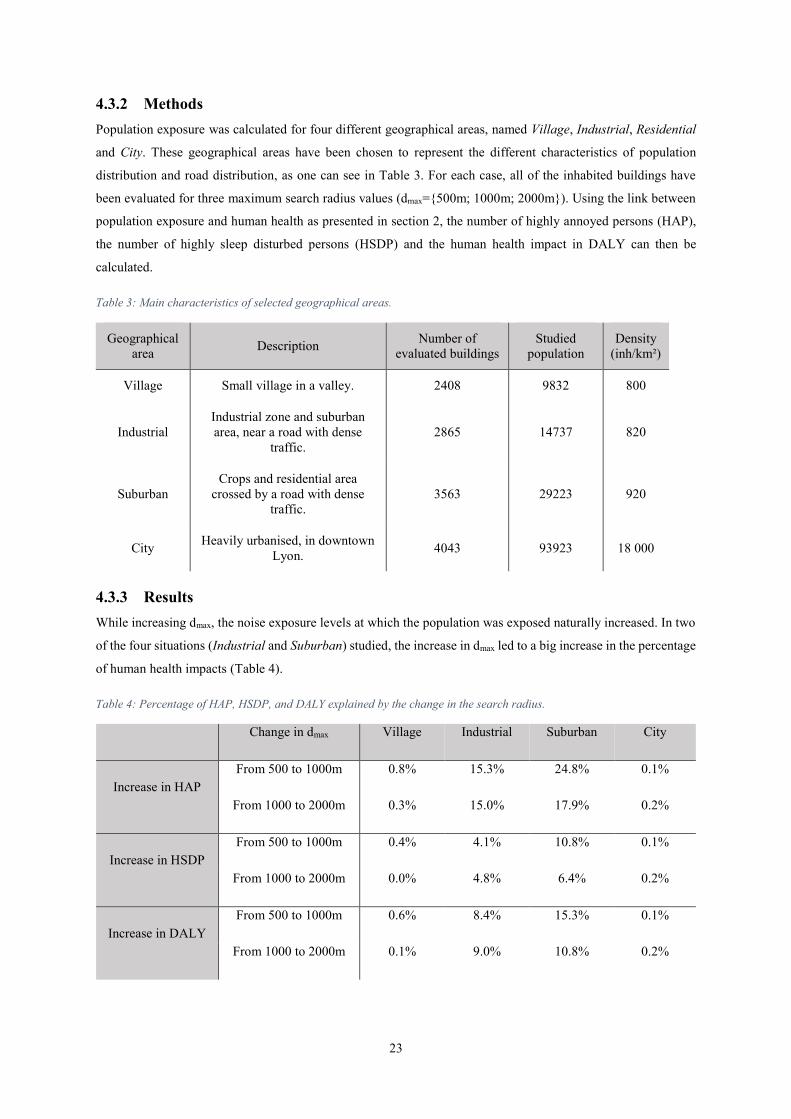
23

4.3.2 Methods

Population exposure was calculated for four different geographical areas, named Village, Industrial, Residential

and City. These geographical areas have been chosen to represent the different characteristics of population

distribution and road distribution, as one can see in Table 3. For each case, all of the inhabited buildings have

been evaluated for three maximum search radius values (dmax={500m; 1000m; 2000m}). Using the link between

population exposure and human health as presented in section 2, the number of highly annoyed persons (HAP),

the number of highly sleep disturbed persons (HSDP) and the human health impact in DALY can then be

calculated.

Table 3: Main characteristics of selected geographical areas.

Geographical area

Description Number of

evaluated buildings Studied

population Density

(inh/km²)

Village Small village in a valley. 2408 9832 800

Industrial Industrial zone and suburban area, near a road with dense

traffic. 2865 14737 820

Suburban Crops and residential area

crossed by a road with dense traffic.

3563 29223 920

City Heavily urbanised, in downtown

Lyon. 4043 93923 18 000

4.3.3 Results

While increasing dmax, the noise exposure levels at which the population was exposed naturally increased. In two

of the four situations (Industrial and Suburban) studied, the increase in dmax led to a big increase in the percentage

of human health impacts (Table 4).

Table 4: Percentage of HAP, HSDP, and DALY explained by the change in the search radius.

Change in dmax Village Industrial Suburban City

Increase in HAP From 500 to 1000m 0.8% 15.3% 24.8% 0.1%

From 1000 to 2000m 0.3% 15.0% 17.9% 0.2%

Increase in HSDP From 500 to 1000m 0.4% 4.1% 10.8% 0.1%

From 1000 to 2000m 0.0% 4.8% 6.4% 0.2%

Increase in DALY

From 500 to 1000m 0.6% 8.4% 15.3% 0.1%

From 1000 to 2000m 0.1% 9.0% 10.8% 0.2%

24

This is a major finding of this work. Despite not having any imposed or recommended value for the dmax parameter

while using noise prediction software can significantly affect the results. Users of said software must be careful

with the chosen value and specify it while communicating the results of their analysis.

Another major result is the presence of two different behaviours. Table 4 shows normalized increases between

4% and 25% for the three indicators in both Industrial and Suburban areas, whereas there is almost no increase

for Village and City areas. The study found that this difference was due to heavily trafficked roads. The presence

of a noise source stronger than the majority of the noise sources in the studied zone can significantly affect the

exposure of the evaluated buildings, particularly when a change in the search radius integrates a heavily trafficked

road in the calculation. Since there is a significant difference between a search radius of 1000m and 2000m, it is

advised to take the largest possible search radius. Although there is no theoretical reason to use 1000m for dmax

instead of 2000m, there is a practical reason. A lot of calculations are not feasible with a search radius of 2000m

because going from 1000m to 2000m multiplies the calculation time by more than 4. An elegant solution for this

particular problem could be to associate a search radius to each road, depending on the emission noise level of

this specific road in absolute terms or compared to other noise sources in the surroundings. This way, an evaluated

building will not consider all the noise sources above a given distance but only the strongest. Applying this

approach in noise prediction software could increase the accuracy of the noise exposure without increasing the

calculation time too much.

All the calculations of the results presented in the following sections have been done with a dmax of 1000m because

it was impossible to do these calculations with a dmax of 2000m. The paper, found in Annex II, goes into further

detail related to the additional calculation time when expanding dmax from 1000m to 2000m. Additionally, this

paper shows that the uncertainties regarding lower noise levels are substantially higher than the ones of higher

noise levels. Because of the logarithmic scale of the decibels, lower noise levels are naturally more sensitive.

4.4 Conclusion

These noise prediction method and software need a lot of information compared to traditional/simpler approaches,

such as the one initiated by Müller-Wenk (1999). However, noise prediction method and software are based on a

finer modelling scale and thus give more accurate and reliable results. For example, the noise exposure of the

population can be accurately assessed instead of using aggregated population data in groups of 5dB(A) ranges as

in Müller-Wenk (1999) or Franco et al. (2010). Reducing population aggregation yields a more detailed

assessment of human health damage. The increase of traffic can also be accurately localised at the road level

instead of imposing a strictly proportional increase over the considered road network as in Franco et al. (2010)

and Müller-Wenk (1999).

Two important simplifications coming from the data and tools have to be underlined. First, population is modelled

based on their place of residence. However, in reality, most of them will not be at home the whole day.

Environmental noise exposure during work, for example, will be accounted for at the residency and not at the

workplace. Secondly, the whole population of a building is constantly allocated at the receptor with the highest

noise emission level. Here, the precautionary principle is applied to avoid underestimation since the precise

location of each person in the buildings is not known. These approximations are already integrated in all other

25

methods using data on population exposure that are generated with the same biases. It does not come from the

integration in LCA but from the data and tools used in the acoustic modelling.

The acoustic knowledge underlying this work has been explained, the existing methods to integrate noise in LCA

have been compared and the principal tool on which this work relies has been explained. It is now possible to

explain in detail the proposed method to develop CFs integrating environmental noise impact on human health in

LCA. This is the objective of the next section.

26

5 Proposed method to develop CFs for environmental noise

impact on human health

Even if cardiovascular disease will not be taken into account in the results due to data limitations (section 2.3.3),

they have been integrated in the methodology. This way, if one has access to the necessary data, one could easily

include this specific health impairment in the calculation along with the other health impairments already

integrated (annoyance and sleep disturbance, section 2.3.1 and 2.3.2).

5.1 Selecting midpoints for this impact category.

As developed in Cucurachi et al. (2014), the best way to include a new impact category in LCIA is to rely on the

mechanistic approach and the indicators put in place by the specialists of this scientific field. Understanding how

environmental noise can affect human health and how this impact is calculated in the state-of-the-art literature

from the acoustician’s point of view (Fritschi et al., 2011; Miedema and Oudshoorn, 2001) allows us to propose

different possible midpoints.

Studying the link between exposure and human health damage reveals thresholds and non-linear effects (section

2). A change in exposure without information on the initial exposure of each individual of the population will lead

to approximations and mistakes. The averaged exposure over the whole population is not sufficient since an

increase in dB(A) will have a different impact depending on the initial noise level at which a population is exposed.

This aspect discourages the use of a midpoint indicator based on a change in exposure because it would not be

representative of the human health effects it intends to represent. A midpoint based on each health impairment

seems the most logical and reliable choice. Annoyance will be quantified in number of HAP and sleep disturbance

will be quantified in number of HSDP.

The logarithmic scale of the human perception level, the complexity of the propagation, the non-linear effects,

and the thresholds in the relationships linking human health and exposure to environmental noise discourages an

aggregated midpoint, such as the one proposed and only used by Cucurachi et al. (2012) in person*Pa*s (number

of people exposed to a certain sound pressure for a certain time duration). In Cucurachi et al. (2014), a framework

is proposed for the inclusion of emerging impacts in LCIA, such as noise. Cucurachi et al. (2014) state, “The

theory should allow for the definition of a clear link between the physical properties of the impact and the effect

that the impact has on the target-subject under study.” Cucurachi et al. (2014) also state that “The model developer

may not proceed any further if clear mechanisms are not yet clearly known or supported by sufficient scientific

evidence.” Yet, in the midpoint chosen by Cucurachi et al. (2012), there is no dose-response relationship between

a human health impact in terms of highly annoyed persons, highly sleep disturbed persons or DALY. An additional

amount of Pa*s would not have an effect on human health depending of:

The source type under consideration, e.g. trains, road traffic and airplanes (Miedema and Vos, 2007;

Miedema and Oudshoorn, 2001). It’s not possible, considering the cause-effect chains, to aggregate

together noise immissions coming from different sources.

The noise levels prior to this additional mount. Low noise levels would lead to no additional impacts on

human health (because of the thresholds). In the interval where the does-response relationships are valid,

impacts of an additional noise immisions decrease with the existing noise background (Miedema and

27

Vos, 2007; Miedema and Oudshoorn, 2001). Summing together Pa*s added to different noise

background will lead to the impossibility to link it correctly to an impact on human health.

This scientific evidence goes against the aggregation of noise from different sources over the whole life cycle as

proposed by Cucurachi et al. (2012). To our knowledge, there are no elements proving that person*Pa*s is a useful

or even viable midpoint. The closest existing unit of measurement is probably pascals-squared-seconds, or

pasques (Pa2*s). Pasques can be used to calculate the noise dose a person receives and can be summed over a long

period, even a lifetime, to evaluate the noise exposure of a given individual (Drott and Bruce, 2011). This metric

is not aggregated over a population, but, even if it was, it is different than the one proposed by Cucurachi et al.

(2012).

Once midpoints have been calculated for each health impairment considered, converting them to the human health

damage endpoint in DALY is a simple step (section 2.1). To do so, the practitioner must multiply each calculated

midpoint with the corresponding disability weights and then sum them together. The result of this operation is an

endpoint given in DALY. The chosen midpoints (health impairments induced by noise) may be perceived far

down in the cause-effect chain, but any aggregation prior to perception step can lead to large errors. Each noise

source type has a different impact due to a difference in interpretation by the human brain, which is why it may

be impossible to define a midpoint prior to this perception step.

As it will be discussed in the section treating the different uncertainty sources (subsection 6.3), one of the larger

uncertainty sources is the conversion from midpoint to endpoint using the disability weights from the acoustic

literature. The uncertainty related to the conversion between health impairments (annoyance and sleep

disturbance) and DALY justifies the differentiation between midpoints and endpoint.

5.2 Calculating a set of CFs for LCIA

5.2.1 Inventory

CFs link LCI EFs to impact categories, thus making LCI processes and EFs the first element to clarify. Since this

methodology focuses on road transportation, a potentially large number of LCI processes are concerned. The

vehicle-kilometre (vkm) metric is used in a lot of LCI processes for road transportation. Other metrics of

transportation found in the LCI, such as ton-kilometres (tkm) or passenger-kilometre (pkm), can be converted to

vkm if the average load is known. When looking at different LCA databases like ecoinvent, GaBi and ELCD

(Frischknecht et al., 2005; GaBi, 2015; JRC, 2016), one can find dozens of processes concerning road

transportation for passengers (e.g. Car petrol…Euro 4, passenger car[vkm]) or goods (e.g. Cargo hauled by truck

[tkm]).

Vkm is a unit of distance and thus does not exactly correspond to the definition of EF stating material or energy.

However, it was used as a proxy for the sound energy emitted by the displacement of vehicle over the quantified

distance. At least two LCIA methodologies include CFs for environmental noise: the Swiss eco-factors 2013

(Frischknecht and Büsser Knöpfel, 2013) and the EPS methodology (Steen, 1999a, 1999b). And both used vkm

as the EF on which they applied CFs for environmental noise. Using a distance-based quantification as already

used in these two methodologies is one possibility, and another option is to use an energy-based quantification.

Joule could be used as a new EF on which to build CFs for the integration of noise impact in LCA. The method

28

proposed here allows the establishment of CFs using these two possibilities for EFs. Distance-based and energy-

based CFs will be compared and the advantages and disadvantages of these EFs will be discussed.

Distance-based. Most of the existing methods (Franco et al., 2010; Moliner et al., 2014; Müller-Wenk, 1999)

calculate human health impact with a distance based approach. Building CFs using such an approach will require

LCI EFs in vkm, and doing so would be quite simple for LCI processes for road transportation. For all these

transportation processes, an output EF of one vkm per one vkm input should be created. For transportation

processes in tkm or pkm, the load factor (mean number of passengers or tons transported by said transportation

processes) has to be taken into account, thus the output EF for one tkm or pkm input would be 1/(load factor).

This additional step will also increase uncertainty since it relies on mean load factor, and that can deviate from

the reality.

Energy-based. In contrast to the distance-based approach, and as developed in (Cucurachi et al., 2012), another

EF on which a CF for noise impact can be build is the sound energy of the considered process (in joule). Sound

energy is obtained by multiplying the sound power of the source (in watts) by the duration of emission (in

seconds). Using sound energy in the LCI requires an additional EF (sound energy in joule) for each process of

road transportation in the database. The sound energy of a given vehicle will depend of various parameters (the

nature of the road surface, the slope of the road, the speed, etc.) and not only of the vehicle itself. These parameters

will unlikely be known for each vkm accounted for in the LCI of an LCA case study, and thus the calculation of

sound energy would be based on a representative average. For transportation processes willing to integrate

environmental noise impact, an output EF in joules has to be defined. Accurately evaluating the output EFs in

joule per vkm for each concerned process will play an important role in the accuracy of the results. Like with the

distance-based approach, dealing with processes in tkm or vkm will add an additional term of 1/(load factor) and

increase uncertainty.

Since LVs and HGVs are separated in the acoustical models, they have to be assessed separately when developing

noise impact CFs. With a distance-based approach, HGVs are noisier than LVs, so differentiating these two types

is a necessity. A difference between these two vehicle types can also exist with an energy-based approach. For

example, LVs and HGVs are spread differently between time periods and within the road networks. In our data,

there is a higher percentage of HGVs on motorways than in city centres and higher percentage of HGVs at night

than during the day. These differences could induce differences in the impact per joule, thus at least two EFs

would still exist: one for LV and another for HGV.

Because the sound energy induced per one vkm of a given vehicle is not constant, using vkm as an intermediary

in the calculation of impacts on human health could lead to significant errors in the assessment. In contrast, an

energy-based logic will simplify the integration among all the different processes in the inventory, conditional

only upon properly defining the EF in joules for each of the processes. An energy-based approach presents

advantages, although the characterisation framework developed here can work with energy-based and distance-

based approaches. The traffic (or its evolution) can be accounted for in vkm or joule resulting in distance-based

and energy-based CFs, and the rest of the cause-effect chain is unchanged, as shown in Figure 1. In the following

methodology, EF will be used to refer both to vkm and joules.

29

Figure 1: Simplified cause-effect chain.

5.2.2 The development of CFs

As already detailed in section 1.1, a CF links an EF to an impact category at the midpoint or endpoint level. A CF

can be calculated by dividing the effect (in our case, human health impact) in an area by the amount of the EF that

produces it (Pennington et al., 2004) (23). The CF for one unit of EF (one vkm or one joule), for one vehicle type

ref, occurring in a geographical area i, during the time period t (e.g. day/evening/night), for a specific health

impairment k (annoyance or sleep disturbance), will be the sum of the considered effect on the exposed people j,

divided by the amount of EF causing it, as stated in (23).

, , , = ∑ , , , ,, , (23)

The result of (23) will be the effect on human health for one health impairment k coming from one unit of EF (e.g.

number of HAP per joule for LVs in the geographical area i and the time period t). The CFs for the different health

impairments k can be aggregated at the endpoint level by linking the inventory item (sound energy) to an impact

on human health in terms of DALY using the disability weights (DW) presented in section 2.1. The result of (24)

is an endpoint CF in DALY per unit of EF for a vehicle type ref located in the geographical area i during the

period t.

, , = ∑ , , , ∗ � (24)

Once the CF has been calculated for a specific geographic area, vehicle type, and time period, it can be used by

any LCA practitioner without any supplementary noise emission and propagation modelling. For example,

environmental noise damage on human health is given in (25) based on (1). It is likely the most efficient way to

integrate noise impact on human health in a systematic and practical way in a classical LCA framework.

� � �� = ∑ ∑ ∑ , , ∗ , , (25)

Due to the logarithmic nature of the human perception of noise and the non-linear effects between exposure and

human health impacts, the impact of one unit of EF will be dependent upon the traffic considered (i.e. the total

amount of EF in the area). There are two possible and different approaches to build these CFs (Huijbregts et al.,

2011): a marginal approach and an average approach. The United Nations Environment Programme (UNEP, 2016)

advises method developers to provide sets of CFs corresponding to both approaches. Since data and method allow

30

it, the calculation of both of the resulting CFs will be compared. Both approaches are schematically represented

in Figure 2.

The marginal approach. The literature concerning the inclusion of noise damage on human health in LCA takes

into account the existing environmental noise, thus only considering the impact of additional traffic. The first

approach by Müller-Wenk (2004, 2002, 1999) considered an additional trip of 1000 vkm distributed over the

entire Swiss road network in proportion to the existent traffic. Franco et al. (2010) took a similar approach by

splitting 1000 vkm over their considered road network (only high-capacity roads). Moliner et al. (2014) measured

the addition of one vkm on several Spanish motorways. Finally, Cucurachi et al. (2012) calculated CFs from the

existing noise background level. To apply a marginal increase to the existing traffic, spreading the additional

traffic proportionally to the existing one is considered to be the most suitable for the inclusion of traffic noise in

LCA (Franco et al., 2010), an approach already adopted by Althaus el al. (2009), Doka (2003) and Müller-Wenk

(2004, 2002, 1999). In this approach, the presence of LVs and HGVs can be increased separately, and thus

distance-based and energy-based CFs can be determined for each vehicle type.

For instance, if an impact category has a high threshold or exponential exposure-response relationship, the last

unit of EF would have a larger environmental impact than the first one. On the contrary, if an impact category

has, for instance, a logarithmic exposure-response relationship, the last unit of EF would have a smaller

environmental impact than the first one. In situation with high environmental pressure, a marginal change is

judged to be virtually irrelevant (Huijbregts et al., 2011). This is a weakness of the marginal approach, and it can

be corrected by the use of an average approach. To our knowledge, the latter has not been developed yet in the

LCA literature for the specific case of environmental noise.

The average approach. An average approach would consist of calculating the entire environmental noise impact

on human health from road transport in a given area divided by the total amount of sound energy from road

transport causing it. Thus, LVs and HGVs cannot be differentiated, and only the total effect of both vehicle types

together is available. The results would be a set of CFs for a given geographical area, for a given time period and

for a given health impairment without the differentiation of the vehicle type. Since there is an important difference

in terms of the emission power level between LVs and HGVs, it seems illogical to aggregate LVs and HGVs with

a distance-based approach. Thus, choosing an energy-based quantification when adopting an average approach is

advised.

In the calculation of the average CFs, the total impact is divided by the total amount of noise causing it. Following

the global guidance for LCIA indicators (UNEP, 2016), the average CFs are calculated taking into account a

situation without human intervention as the reference state, i.e. without noise from road transportation. That is

why the average approach curve represented in Figure 2 starts at the origin. This is different from the so-called

“zero-effect” approach where the average approach would have started at the first detectable impact (origin of the

exposure-response curve) instead of the origin (Huijbregts et al., 2011). This aspect will be further discussed in

subsection 7.7 as well as the practical uses of both average and marginal approaches.

31

Figure 2: Schematic representation of both marginal and average approaches.

For the impact assessment researchers, both approaches are thought as complementary and will allow different

interpretations of the impact category under study. The marginal approach will give the impact for an additional

amount of EF while the average approach will give the impact per unit of EF. Moreover, comparing marginal and

average CFs can also give an idea of the sensitivity of marginal CFs to the existing state in which they have been

calculated. If there is a big difference between average and marginal CFs, a change in the reference situation in

which the marginal and average CFs were calculated would have a big impact on the value of these CFs. As a first

approximation, the lower the difference between the two, the lower the sensitivity of the amount of EF in which

the CFs were calculated.

5.2.3 Health impairment and time periods

The existing dose-response relationships link sleep disturbance to Lnight, noise annoyance to Lden and

cardiovascular disease to Lday,16h, as summarised in Figure 3. The three health impairments considered concerned

night, the whole day or the day and evening periods. Based on the health impairments considered, the CFs for the

evening and day periods cannot be differentiated, and thus the CFs will only be defined for the night period (22h

to 6h) and the day/evening period (6h to 22h).

Figure 3: Health impairments considered and their link with noise indicators.

32

Environmental noise assessment is based on hourly traffic, but the impact of environmental noise on human health

is calculated over one year. When normalizing with the marginal approach and vkm as EF, the total amount of

vkm will be the increase of vkm on the hourly scale ∆traffic multiplied by the number of hours in the daytime

period and the number of days in one year. For example, (26) shows how to calculate the marginal increase of

traffic ∆vkm(t) over one year where Hi is the number of hour in the time period i and year is the number of days

in a year. ∆ , ℎ = ∆ , + ∆ , + ∆ , ℎ= year ∗ ∑ ∆ � ∗ (26)

For sound energy, the calculation relies on the sound emission level Lw/m per metre of lane. The sound power W/m

can be calculated as show in (27) where W0 is the reference sound power of 10-12 watts.

�/ = � ∗ � / (27)

If a section of roads at a noise emission power per metre W/m is multiplied by the total length of this section, a

noise emission power is obtained in Watts. At this step, noise emission power from all the sections can be added

together, leading to a global noise emission power for the whole road network under consideration W. The last

step to obtain the sound energy is to multiply this noise emission power by the time under consideration. In (28),

the marginal increase of sound energy ∆E(t) is calculated from the increase in sound emission power ∆W(t), which

is calculated from the increase in hourly traffic (difference between W with and without an increase in traffic).

When taking an average approach, the whole sound energy in the area of study will be accounted for instead of a

marginal increase, as detailed in (29). ∆ , ℎ , ℎ = ∆ , + ∆ , + ∆ , ℎ= ∗ ∗ ∑ ∆� ∗ (28)

, ℎ , ℎ = ∗ ∗ ∑ � ∗ (29)

The resulting midpoint CFs for annoyance for all periods (day, evening and night) is seen in (30). The number of

HAP is derived from the exposure of the population (associating persons and the exterior noise exposure levels at

the most exposed façade of their dwelling) and the dose-response relationship for noise annoyance based on the

exterior noise exposure levels at the most exposed façade (Miedema and Oudshoorn, 2001). It is important to note

that this dose-response relationship is only valid for Lden ranging between 45 and 75 dB(A). Persons exposed to

levels lower than 45 dB(A) are not considered. Persons higher than 75 dB(A) are evaluated at 75 dB(A), i.e. at

the maximum of the range.

= , ℎ (30)

33

With a marginal approach the Number of HAP taken into consideration would be the additional number of HAP

due to the increase of traffic and the EF will be quantified with (26) for distance-based CFs and with (28) for

energy-based CFs. With a marginal approach the Number of HAP taken into consideration is the whole number

of HAP in a given area and the EF will be quantified with (29) in the same area.

The same logic, when applied to sleep disturbance, leads to a CF only valid at night, as expressed in (31). Here,

the additional number of HSPD is derived from the exposure of the population and the dose-response relationship

for sleep disturbance (Miedema et al., 2002). This dose-response relationship is valid for Lnight and ranges between

45 and 65 dB(A). Persons exposed to Lnight below 45 dB(A) are not considered while persons exposed to Lnight over

65 dB(A) are evaluated at 65 dB(A).

= , ℎ (31)

Doing the same for cardiovascular disease yields a CF valid for the day and evening, as expressed in (32) for non-

fatal cardiovascular disease and in (33) for fatal cardiovascular disease.

= � � � � �, + , (32)

= �� � � � � �, + , (33)

With the three health impairments considered, only two periods can be differentiated: day/evening and night. The

resulting CFs in DALY for these periods are detailed in (34) and (35), where previous CFs are multiplied by the

corresponding disability weight DW. Depending of the choice of EF, the resulting CFs are distance-based or

energy-based.

{ , } = ∗ � + ∗ � + (34)

ℎ = ∗ � + ∗ � (35)

For simplification, the day and evening periods (from 6 a.m. to 10 p.m.) will be labelled as day in the following.

Endpoint CFs for the day will stand from 6 a.m. to 10 p.m. and endpoint CFs for night will stand from 10 p.m. to

6 a.m.. For simplification and concision, midpoint CF for annoyance will be labelled as HAP and midpoint CFs

for sleep disturbance will be labelled as HSDP.

5.2.4 Geographical area

The considered geographical areas play another key role in creating a relevant CF. With the method developed

here, one can accurately calculate the marginal effect on human health due to an increase in traffic in a well-

known geographical area. If desired, the level of detail can be fixed to a single road, which is an alternative and

potentially more detailed approach than the one developed by Ongel (2016), where the CFs proposed for nine

34

Turkish municipalities were based on main arterial roads. One could also produce georeferenced CFs based on a

normalised grid of a given territory, as in Cucurachi and Heijungs (2014). Of course, such an approach will need

a huge amount of effort if the CFs have to be calculated for all the roads worldwide or even for a larger

geographical subunit (e.g. a 5×5 km² grid). For now, the available data mostly concerns big cities and calculating

CFs for a whole country or at the European level could be very difficult, if not impossible. Moreover, it can be

problematic for the practitioner to know where a given transport is occurring, and the usefulness of explicitly

georeferenced CFs is questionable. An exception to this is in specific cases, such as a comparison between two

roads. In this case, specific modelling in a noise prediction software may be the best solution. When establishing

CFs, one has to take into account that the inventory processes considered by the practitioner are not often

accurately localised.

Cucurachi et al. (2012) and Cucurachi and Heijungs (2014) propose a good compromise by using archetypical

conditions. These archetypes are predefined models judged to be representative of various situations. Cucurachi

and Heijungs (2014) used six different geographical archetypes: urban, suburban, rural, industrial, indoor and

unspecified. The authors attest to an accounting of noise emissions over the whole life cycle, and that these CFs

could be used for all kind of noise emissions and not only for road transportation. This aggregation is problematic

as discussed in 5.1 and will be further addressed in the discussion (subsection 7.1). Using archetypal conditions

is interesting because it allows one to calculate a set of CFs that can then be used easily by an LCA practitioner.

Once the CFs have been calculated, they can be used in a systematic way in the basic framework of LCA without

needing any additional modelling. For this reason, the archetypal approach seems the most appropriate to address

noise impacts if one wants to take into account the variety of effects between different geographical areas. Instead

of fixing archetypes a priori, another approach could be to calculate the proposed CFs in various situations and

then identify different types depending on the outputs’ variations, an a posteriori approach.

For this application, a division of the French territory into a set of IRIS (Ilots Regroupés pour l'Information

Statistique - Aggregated Units for Statistical Information), was chosen. IRIS is one of the levels of collection and

transmission of statistical data coming from the French National Institute of Statistics and Economic Studies

(INSEE) (Institut national de la statistique et des études économiques). These geographical areas are on the district

scale and contain between 1800 and 5000 people. They are built in a way that ensures homogeneity among

geographic and demographic criteria, which is precisely why this mapping has been chosen. Moreover, they are

small enough to allow for a lot of different calculations leading to a large amount of results that can be statistically

analysed. At the same time, they are also large enough to have hundreds of buildings evaluated for each situation

ensuring a correct “signal” and not some random statistical “noise”. Due to the way they are built, IRIS do not

have all the same form or the same surface. However, if the effects of the surroundings are correctly taken into

account, this aspect should not be problematic.

If significant differences are found while calculating the CFs among different geographical areas, it may be

possible to establish different types and to define typical CF values (and in the best case uncertainty distributions)

for each identified type. While creating geographical subunits, the IRIS cutting was preferred to ensure

homogeneity of the studied areas, but a normalised grid could also have been used. This method can be used on

any geographical area.

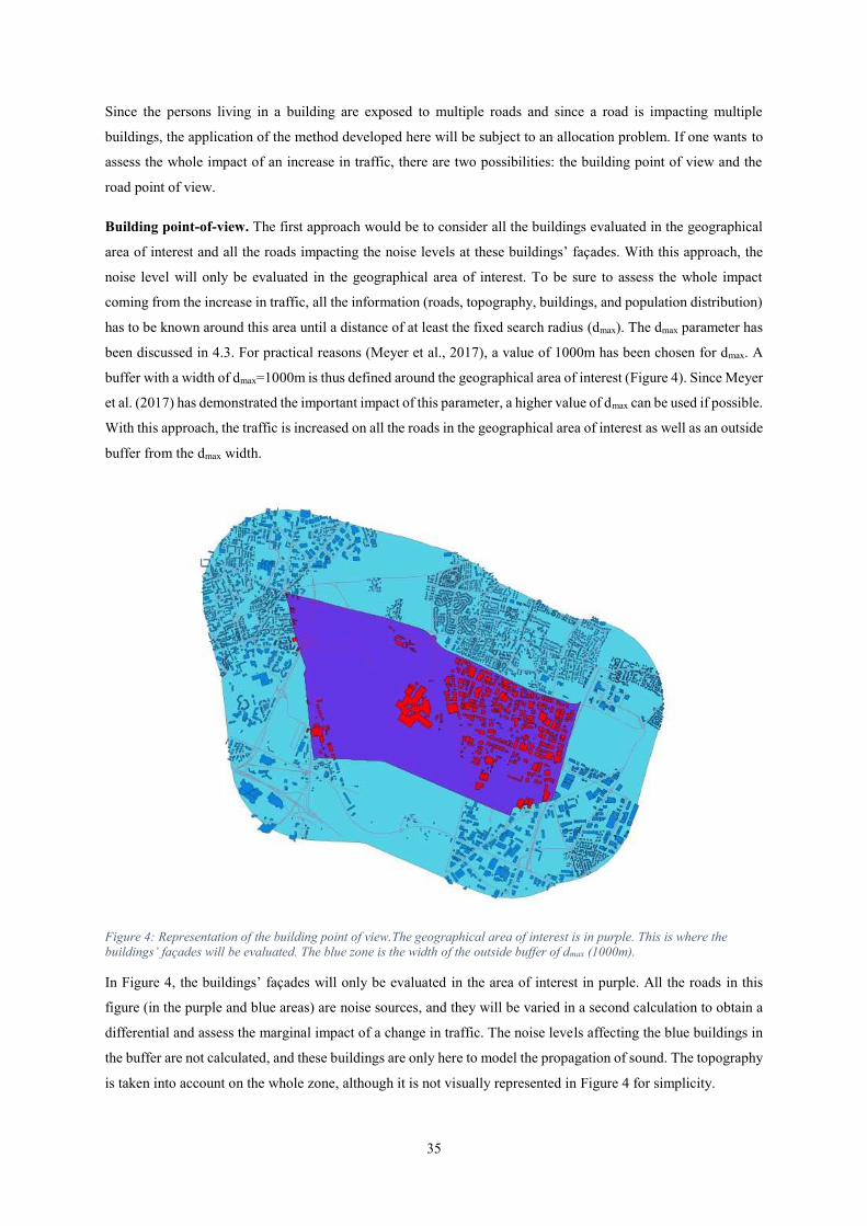
35

Since the persons living in a building are exposed to multiple roads and since a road is impacting multiple

buildings, the application of the method developed here will be subject to an allocation problem. If one wants to

assess the whole impact of an increase in traffic, there are two possibilities: the building point of view and the

road point of view.

Building point-of-view. The first approach would be to consider all the buildings evaluated in the geographical

area of interest and all the roads impacting the noise levels at these buildings’ façades. With this approach, the

noise level will only be evaluated in the geographical area of interest. To be sure to assess the whole impact

coming from the increase in traffic, all the information (roads, topography, buildings, and population distribution)

has to be known around this area until a distance of at least the fixed search radius (dmax). The dmax parameter has

been discussed in 4.3. For practical reasons (Meyer et al., 2017), a value of 1000m has been chosen for dmax. A

buffer with a width of dmax=1000m is thus defined around the geographical area of interest (Figure 4). Since Meyer

et al. (2017) has demonstrated the important impact of this parameter, a higher value of dmax can be used if possible.

With this approach, the traffic is increased on all the roads in the geographical area of interest as well as an outside

buffer from the dmax width.

Figure 4: Representation of the building point of view.The geographical area of interest is in purple. This is where the

buildings’ façades will be evaluated. The blue zone is the width of the outside buffer of dmax (1000m).

In Figure 4, the buildings’ façades will only be evaluated in the area of interest in purple. All the roads in this

figure (in the purple and blue areas) are noise sources, and they will be varied in a second calculation to obtain a

differential and assess the marginal impact of a change in traffic. The noise levels affecting the blue buildings in

the buffer are not calculated, and these buildings are only here to model the propagation of sound. The topography

is taken into account on the whole zone, although it is not visually represented in Figure 4 for simplicity.

36

The building point-of-view is simple and may appear as a viable approach to establish CFs, but there is a major

problem: to assess the human health impact per a unit of traffic, the whole human health impact calculated here

is divided by the increment in vkm. However, all the roads included in a band of ± dmax of the IRIS’ border will

be common in the calculation of several IRIS. This means that to avoid an underestimation of the midpoint CFs,

the impact of the increment of the shared roads have to be allocated between concerned IRIS. There is no easy

way to solve this allocation problem. The building point-of-view is not suitable to determinate the potential impact

of a marginal emission increase. The building point-of-view will not be used in this work since this receptor

perspective induces non-negligible errors that may be avoided from a second approach: the road point-of-view.

Road point-of-view. This approach considers the roads and not the buildings, thus varying the traffic on the roads

contained in the IRIS. The aim is to find the total impact of the roads in the IRIS and only increase the traffic on

these roads. To do this, the buildings in the IRIS, plus the ones within dmax from the border of the IRIS, have to

be evaluated because they are affected by the increase in road traffic inside the IRIS. To have a correct measure

of the buildings in the internal buffer in light blue (Figure 5), an external buffer in white is needed in order to fix

the environmental background noise of the internal buffer. Both buffers have a width of dmax.

Figure 5: Representation of the road point of view.The purple area is the one where the CFs are calculated. The area in blue

is the internal buffer. Noise exposure levels are calculated for all the buildings in red, while the road traffic is only increased

in the purple area.

37

In Figure 5, the CFs are calculated for the purple area. To assess these CFs, two calculations are needed: one with

and one without a traffic increase. With the road point-of-view, the road traffic will only be increased in the

geographical area in purple. All the buildings in red (in the central area and internal buffer) will be evaluated

because they are located less than the dmax of a road on which traffic has been increased. The road traffic in the

internal and external buffers will not be increased between the two simulations, but they have to be here as noise

sources to fix the environmental noise for a correct calculation of the noise exposure levels. The buildings in the

external buffer are only here for their impact on the sound propagation. The topography is taken into account for

the whole area, although this is not shown on the figure for simplicity.

This approach does not need any allocation. It simplifies this problem from the building point-of-view and avoids

a major source of errors. This approach only implies a small error in the calculation, and this is because the

logarithm of the sum is lower than the sum of the logarithm. The sum of the increase in noise levels found at a

building’s façades shared between several calculation areas (i.e. in a band of ± dmax of the IRIS’ border) will be a

little bit higher than the increase in noise levels found if the traffic roads are increased simultaneously in all the

IRIS. The road point-of-view is preferred to the building point-of-view. Thus, this approach should be the one

used while applying this method and is the one used in the rest of this work.

5.2.5 Practical considerations for the marginal approach

Adding only one vkm (or even 1000) in the whole studied system over a year will not affect the outputs of noise

prediction models in any measurable way; it is also not even possible since noise prediction software simulates

road traffic hourly. For example, when Franco et al. (2010) added 1000 vkm on the road network they considered,

it led to an increase of roughly 10-8 additional vehicles per hour. In the noise prediction software, even a single

increment in hourly traffic will produce several hundreds of vkm over one year. The methodology developed here

forces the practitioner to increase the traffic in a larger amount than preceding methods, but the question of the

extent of this marginal increase remains.

To answer this question, five different IRIS around Lyon have been selected, where each represents a different

situation. These geographical areas are different than the ones used to assess the maximum search radius (Section

4.3). The first area, referred to as dense urban, is in the heart of the city of Lyon and is densely populated. The

second area, referred to as urban, is partly exposed to the traffic of the ring of Lyon (more than 4000 vehicles/hour

on both sides during daytime). A small town was chosen in the periphery of Lyon as the third geographical area

to study, consisting mainly of residential buildings surrounded by fields. This area, referred to as noisy peri-urban,

is exposed to the environmental noise of motorways in the direct neighbourhood. For a fourth comparison, a

similar city in the periphery of Lyon was chosen in a more hilly landscape. This time, the area, referred to as quiet

peri-urban, is less exposed to high traffic roads, and the environmental noise is lower than in the previous case.

Finally, a geographical area was selected in the countryside. The area, named rural, contains small towns, vast

fields and roads with medium density traffic in between. These geographical areas are not thought to be

representative of all the possible situations that one can encounter when studying the marginal impact of

environmental noise. However, these geographical areas have been selected to partly analyse the existing

variability. For each geographical area, the additional number of HAP resulting from the increase in traffic were

calculated using an increase of 11%, 25%, 43% and 67% for LVs and the road point-of-view explained in the last

38

section. The multiplication factor applied on the traffic can only take discrete values (1/0.9, 1/0.8, 1/0.7… etc.)

because of constraints in the CadnaA noise prediction software.

Calculations were conducted on a server equipped with the operating system “Windows Server 2008 R2

Enterprise”, Intel® Xeon™ CPU 3.20 GHz (8 cores) processor and 34.0 GB RAM. The calculation time to

produce a CF varies between a several hours and a few days, depending on the situation.

Figure 6: The additional number of HAP for five different geographical areas (urban, noisy peri-urban, quiet peri-urban,

urban and dense urban) and linear trend line as a function of the multiplication factor applied to traffic of LVs.

In Figure 6, there is a clear linear tendency between the additional number of HAP and the increased proportions

of the studied traffic (R²>0.99 in these five geographical areas). In the range tested here, the CFs will be assumed

as independent of the choice of the multiplication factor. One can also see that the additional number of HAP is

dependent on the geographical area. This aspect will be further studied in subsection Error! Reference source

not found. examining the spatial variability of the results.

5.3 Conclusion

CFs are thought to be the most practical way to integrate environmental noise impact on human health. Here, a

full method has been developed in the case of road transportation. This method allows the derivation of CFs with

an average or marginal approach. The average approach gives CFs in HAP per joule and HSDP per joule at the

midpoint level and DALY per joule at the endpoint level. The usage of these average CFs will be further discussed

later. Marginal CFs are preferred in the LCA framework and are especially useful when looking at small changes

in an operating system. Marginal distance-based and energy-based CFs can be calculated at both midpoint and

endpoint levels. Marginal CFs can also be calculated separately for each vehicle type. These possibilities should

allow further access to interesting information.

R² = 0.9986

R² = 0.9987

R² = 0.9984

R² = 0.9999

R² = 0.9941

0

10

20

30

40

50

60

70

80

90

100

1 1.1 1.2 1.3 1.4 1.5 1.6 1.7

Add

itio

nal n

umbe

r of

hig

hly

anno

yed

pers

ons

Multiplication factor applied to the traffic of light vehicles (LVs)

urban

dense urban

rural

noisy peri-urban

quiet peri-urban

39

This method will now be applied in different geographical situations to see how the values of the CFs are evolving

and if a typology usable in an LCA framework emerges from this analysis.

40

6 Results

6.1 Number of experiments and IRIS choice

Now that the development of CFs for environmental noise impacts on human health have been methodologically

explained, the CFs can then be fully calculated for the region of the Great Lyon. As explained, two buffers are

needed to apply the developed method. An internal buffer in which noise exposure is assessed but the road traffic

is not increased and an external buffer that is only here to fix the environmental noise. In the external buffer, the

road traffic is not increased and the population exposure is not assessed. The necessity to have these two buffers

reduce the surface on which this method can be applied. Only IRIS with internal and external buffers fully

described by the data used were kept as potential candidates for the calculation. This corresponds to 435 IRIS in

the Lyon area, accounting for 339 km² of the 736 km² in the initial area considered. Among these 435 IRIS, some

of them have been selected to cover different geographical situations.

All the calculation in an IRIS take a lot of time. Due to time constraints, the calculation was only conducted on

77 IRIS among the 435 possible ones. The best way to maximise the different situations and eventual types with

a limited sample was to cover a large territory. That is why IRIS have been selected trying to maximise the distance

between them. Of the 77 IRIS calculated, 11 were taken away after the calculation. Under examination, three of

them showed incoherencies in the results and/or a problem in the inputs leading to unreliable results. One other

IRIS had no HGVs at all. In order to compare CFs on HGVs and LVs on the same sample, this IRIS was

eliminated. Six IRIS had no population, or almost no population because those IRIS corresponded to hospitals

(hospitals have specific IRIS and the population is fixed to zero since nobody is permanently living in the hospital)

or working areas (industrial areas or areas consisting only of office buildings). This is the direct consequence of

an important limit of the models and data used: all the inhabitants are located at their place of residence.

Considering unrealistic that nobody is exposed to noise in industrial areas, areas consisting only of office buildings

or hospital, these IRIS can be considered as outliers and were left out of the rest of the calculation. The place of

residence limitation and its possible consequences will be discussed in subsection 7.3.3. Figure 7 shows the total

area considered and includes all the IRIS for which data was available as well as the 435 IRIS with sufficient data

to make the application of the developed method possible. The remaining 67 IRIS that will be analysed in this

section are also presented in Figure 7. These 67 IRIS cover 38.7 km², contain 176,488 people, and over one year,

944 millions vkm of LVs, 48.2 millions vkm of HGVs or 848 millions joules (without considering the buffers).

For each of the geographical areas, a simulation was run in a first scenario (i) without any modification and in a

second scenario (ii) with an increased hourly traffic of 11.1% in LVs or 10.0% in HGVs. The values of increase

are different for LVs and HGVs due to technical constraints in the noise prediction software. These values are the

smallest ones allowing to increase one vehicle type without increasing the other. As detail in the method, the road

traffic is only increased in the IRIS itself (road-point-of-view, subsection 5.2.5). In both cases, the noise exposure

levels Lday, Levening, Lnight and Lden resulting from the whole traffic in the IRIS and the two additional buffers have

been calculated for every inhabited buildings in the IRIS and the internal buffer. The marginal CFs are obtained

by dividing the difference in human health impact between (i) and (ii) by the increase in traffic added in (ii). This

increase can be in LVs or HGVs and can be quantified in terms of energy (J) or distance (vkm) leading to energy-

based or distance-based CFs. The average CFs can directly be calculated from (i). Since we have the traffic in the

41

IRIS and the two buffers and the exposure of the population in the IRIS and the internal buffer, the average CFs

can be calculated on the IRIS alone, on the internal buffer alone, or on the IRIS and the internal buffer together

referred to as extended as show in Figure 8. To calculate these average CFs, the whole impact in an area is divided

by the whole sound energy produced in this area over a year.

Figure 7: Geographical areas considered. In dark blue are the 67 IRIS on which the CFs have been calculated. In mid-weight

blue are the 435 IRIS that could have been used to calculate CFs, and in the lightest blue are the IRIS for which data were

available but without data for the buffers, the calculation with the method developed in this work was not possible.

Figure 8: Schematic representation of the IRIS and the two buffers.

42

No IRIS area is shared with another IRIS. However, when taking into account the internal buffers, geographical

areas are shared. It is not a problem or a source of concern in the calculation of marginal CFs since the method

avoids any effect from the surroundings. However, this point will be discussed while looking at the average CFs

and thus should be underlined. Internal buffers and their superposition are represented in Figure 9.

Figure 9: The 67 IRIS are represented in blue and their internal buffer in grey.

Since many different CFs will be manipulated in the rest of this work, Figure 10 was made for disambiguation

purpose.

43

Figure 10: Summary of the CFs notation.

6.2 Spatial variability of the raw results

Since the method was successfully applied on 67 geographical areas, 67 values are available for each CF. The

resulting spatial variability will be presented and analysed in this subsection. By summing the area of all 67

calculated IRIS, a surface area of 38.7 km² is found among the 339 km² available to apply this method. It means

that a little bit more than a tenth of the potential area was effectively used due to time constraints.

6.2.1 Qualitative approach of the spatial variability of CFs for annoyance

The amount of traffic can greatly vary between IRIS. From the emission perspective, it would be misguided to

consider that all IRIS have an equal weight. To have a first idea of the spatial variability among the 67 IRIS while

taking into account the heavier importance of IRIS with more traffic, the weighted histograms of the different CFs

have been plotted (Figure 11), with the weight being the EF under study. For example, the height of a bar in Figure

11 for CFavg,HA,IRIS (e) is the part of sound energy being produced by the whole traffic during the whole day over

a year in scenario (i) in all the IRIS for which the CF values are contained in the width of said bar.

44

Figure 11: Weighted histograms of the CFs at midpoint level for annoyance.

Figure 11 shows that the major part of the traffic or sound energy is associated with lower values for all the

represented CFs. To ease the analysis of these histograms, it may be better to plot them on a logarithmic scale

instead of a linear one. To facilitate this comparison, the x-axis and the breaks of the weighted histograms are the

same for all the six sets of CFs represented in Figure 12. A decimal logarithm log has been used to quickly interpret

the order of magnitude.

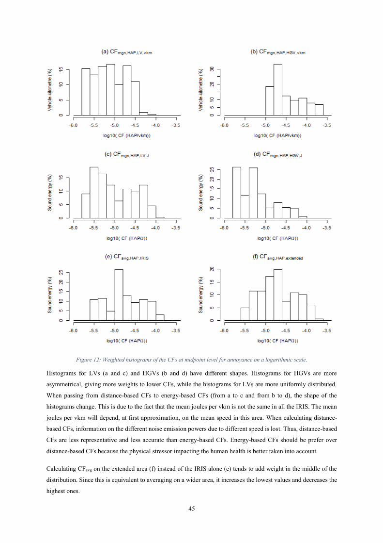
45

Figure 12: Weighted histograms of the CFs at midpoint level for annoyance on a logarithmic scale.

Histograms for LVs (a and c) and HGVs (b and d) have different shapes. Histograms for HGVs are more

asymmetrical, giving more weights to lower CFs, while the histograms for LVs are more uniformly distributed.

When passing from distance-based CFs to energy-based CFs (from a to c and from b to d), the shape of the

histograms change. This is due to the fact that the mean joules per vkm is not the same in all the IRIS. The mean

joules per vkm will depend, at first approximation, on the mean speed in this area. When calculating distance-

based CFs, information on the different noise emission powers due to different speed is lost. Thus, distance-based

CFs are less representative and less accurate than energy-based CFs. Energy-based CFs should be prefer over

distance-based CFs because the physical stressor impacting the human health is better taken into account.

Calculating CFavg on the extended area (f) instead of the IRIS alone (e) tends to add weight in the middle of the

distribution. Since this is equivalent to averaging on a wider area, it increases the lowest values and decreases the

highest ones.

46

In these six histograms, there are a less than two orders of magnitude between the minimum and maximum values

for a given CF. Looking at the ratio of the bounds of the 95-percentile confidence interval in Table 5, values

ranging from 15 to 38 are found. The calculation has been made while weighting the values found in the different

IRIS as explained before for the weighted histograms.

Table 5: Ratio of the bounds of the 95-percentile confidence interval for all the CFs concerning the annoyance midpoint

indicator.

CFmgn,HAP,LV,vkm CFmgn,HAP,HGV,vkm CFmgn,HAP,LV,J CFmgn,HAP,HGV,J CFavg,HAP,IRIS CFavg,HAP,extended . �. � 18 15 33 28 38 38

The values contained in the 95-percentile confidence interval cover between one and two orders of magnitude. It

could justify the elaboration of a typology with CFs calculated for each identified type. For example, if the CFs

calculated in the city are significantly different than the one calculated in the suburbs, different CFs could be

proposed for these two different types. To establish typology a posteriori, the key variables piloting this spatial

variability should be understood, and this is attempted in the next subsection (6.2.2). For a trial analysis, we will

focus on the CFmgn,HAP,LV,J before extending the analysis to the rest of the set of CFs.

6.2.2 Understanding the key variables behind the spatial variability of CFmgn,HAP,LV,J

The GIS layers used as inputs contain a lot of different variables. These variables can be explained explicitly (in

attributes of the layers) or implicitly (population density can be calculated from these GIS layers). By knowing

these input variables and the intended output, one can try to identify the explanatory variables for the observed

variability of the different CFs. The impact of road traffic noise on human health should, at first approximation,

be linked with two input parameters: the noise emission due to road traffic noise and the number of people exposed

to these noise sources.

The noise emission due to road traffic noise can be approximated by sound energy. Using vkm is more prone to

errors because the joules emitted per vkm vary, as observed earlier. Since all the IRIS do not have the same size,

the geographical variable of interest is not sound energy itself but rather the density of the sound energy (j/km²).

The density of sound energy is calculated by dividing the amount of sound energy emitted over a year by the area

in which it is calculated. Calculating the sound energy over a year was chosen in order to stay coherent with the

rest of this work. The second input parameter is the population density. While doing the calculation on an IRIS,

the population exposure is assessed in the IRIS itself and in the internal buffer. The roads are known in the IRIS,

in the internal buffer and in the external buffer. In other words, the population density dpop (pop/km²) can be

calculated in the IRIS and in the internal buffer while the density of sound energy dj (j/km²) can be calculated in

the IRIS, in the internal buffer and in the external buffer. These five variables have been calculated, and a first

test has been done to understand the extent to which these variables could explain the studied output: CFmgn,HAP,LV,J.

Considering the logarithmic nature of the human perception, the existence of thresholds, and the form of the

exposure-response relationship between human health and noise exposure, non-linear behaviours were expected.

The lm function in the R software (R Core Team, 2015) allow to fit linear models using the QR factorisation

47

method. Using it, a first attempt was made to create a linear model between the natural logarithm ln of the CF and

the natural logarithm of these five variables. The lm function was able to produce a linear model with an adjusted

R² value of 0.92. The adjustment of the R² value used Wherry’s formula and quantified how much the variance in

y (ln(CFmgn,HAP,LV,J) in this case) is accounted for when using a predictive model (Andy Field and Miles, 2012).

This first modelling only found three significant variables (p-value < 0.001 for these three variables): the

logarithm of the population density in the IRIS dpop,IRIS, the logarithm of the population density in the internal

buffer dpop,int buf and the logarithm of the sound energy density in the IRIS dJ,IRIS. However, the correlation

coefficient r between dpop,IRIS and dpop,int buf is 0.80, these two variables are redundant and it may be better to only

keep one out of the two. It makes more sense to keep dpop,IRIS since it is the population density in the calculation

area. Moreover, keeping dpop,IRIS lead to a better fitting. The correlation coefficient r between dpop,IRIS and dJ,IRIS is

0.24, these two variables are poorly correlated. Then the lm function was rerun with only these two variables to

obtain a simpler model. In the following these simple models would be referred as surrogate models (SMs).

Surrogate models are models that mimic the behaviour of the simulation model as closely as possible while being

computationally cheaper. An adjusted R² of 0.86 was obtained for the SM specified in (36).

ln( , ��,��, ) = − . + . ∗ ln( , ) − . ∗ ln , (36)

This equation with the logarithm of the output and the logarithm of the variables may not be simple to analyse.

To better understand what is happening, (37) is obtained by applying the exponential function to (36).

, ��,��, = . − ∗ ,.,.

(37)

Essentially, a higher population density in the area of calculation will lead to a higher CF. If one fixes the amount

of sound energy and increases the population exposed by these noise emissions, one can expect an increase in

human health damage. In (37), the relation between the CF and the population density is almost linear and it makes

sense, doubling the population, ceteris paribus, would double the human health impacts and thus the calculated

CF. However, the link between the CF and the density may have been non-linear because while increasing the

population density, other things change, such as the habitation structures (buildings next to the road instead of

houses at several meters) or the nature of the ground (more concrete and thus less sound absorbed by the ground).

Equation (37) also implies that a higher sound energy density in the area of calculation will lead to a lower CF.

Increasing sound energy density, ceteris paribus, leads to higher human health impact. However, to calculate a

CF, the amount of impact is divided by the amount of EFs causing it. Increasing the sound energy density will

then both increase the numerator and the denominator. When looking at the exponent associated with dJ,IRIS, the

normalization effect is stronger than the increase in human health impact due to an increase in the sound energy

density.

Instead of using a linear model for the logarithm of the output and inputs, a non-linear model can be used for the

data. It is possible to do so using the nls function in R. Specifying the starting estimates using the solution found

with the linear model helps to find a solution for the non-linear model. Such a model gives the equation displayed

in (38).

48

, ��,��, = . − ∗ ,.,.

(38)

The result of the non-linear model (38) is quite different from the result obtained while applying a linear model

for the logarithm of both output and variables (37). To better understand what this difference means and where it

comes from, CFs obtained with the noise emission and propagation models (NEPM), our raw results, have been

plotted against the ones obtained with the SMs (37) and (38) for both approaches (Figure 13). Since the linear

scale does not represent the range of CFs well, the logarithm of the NEPM-based CFs have also been plotted

against the logarithm of the SM-based ones for both approaches.

Figure 13: SM-based and NEPM-based CFmgn,HAP,LV,J using linear model (a) and (b) or non-linear one (c) and (d). y=x curve

has been plotted to ease visualisation.

To estimate the quality of the fit, the square of the Pearson correlation coefficient r² was used. The value of r²

between NEPM-based CFs and SM-based CFs is 0.74 for (a) and 0.84 for (c). As expected, and visible in Figure

r² = 0.74 r² = 0.86

r² = 0.84 r² = 0.73

49

13, the non-linear model applied on the raw data fits better than the linear model applied on the logarithm of the

data. The value of r² between the logarithm of the NEPM-based CFs and the logarithm of the SM-based ones is

0.86 for (b) and 0.73 for (d). The first model minimises the relative error while the second model minimises the

absolute error. The average relative error between NEPM-based and SM-based values with the first model is

28.7% while it reaches 43.0% with the second model where lower values are poorly estimated (d). It is preferable

to minimize the relative error than the absolute error because this approach treats the whole range of the CF fairly

instead of overweighting the higher values. The first approach using the linear model on the logarithm of the

variables is thus the preferred one.

The outlier in Figure 13 (a) is better explained while taking into account dpop,int buf . The inability of the SM to

predict this value is thus coming from a significant difference between the population density in the IRIS and in

its neighbourhood. However, adding another variable to the SM to better predict one outlier and have marginal

improvement on others does not seem worth it and could be a disputable choice since dpop,int buf and dpop,IRIS are

highly correlated.

When comparing the outcomes of (37) and (38) in Figure 13, one can see that the power of both dpop,IRIS and dJ,IRIS

have decreased. While it allows for a better fit of higher CF values, it also leads to poor estimations of low values

with the second SM (Figure 13 (d)). Lower values seem to be more sensitive to dpop, IRIS and dJ,IRIS than higher ones.

These two values seem to evolve together, however they are not correlated, as stated before the correlation

coefficient r between dpop,IRIS and dJ,IRIS is 0.24 (r² is 0.06).

In Figure 14, CFmgn,HAP,LV,J has been plotted against the population density calculated over the IRIS (a) and the

sound energy density calculated over the IRIS (b), since they are the two most important variables. Even if there

are visible tendencies, it is hard to identify subgroups that could correspond to a possible typology. When looking

at population density, for example, where should be the cut-off between two eventual types? Should we use the

model found above to distinguish different type? In this case, a complex ratio between the population density and

the sound energy density would not be practical for the LCA practitioner filling out an LCI because of data limits,

complexity and comprehensiveness.

Figure 14: CFmgn,HAP,LV,J plotted against the population density calculated over the IRIS (a) and the sound energy density

calculated over the IRIS (b).

50

Looking at CFmgn,HAP,LV,J shows how difficult it can be to establish a typology but, maybe, establishing such a

typology is not possible, useful or practical. In Figure 15, the value of CFmgn,HAP,LV,J is represented by shades of

grey in the IRIS in which they are calculated; darker shades of grey correspond to higher values of CFmgn,HAP,LV,J.

Figure 15: Geographical representation of the 67 IRIS and associated CFmgn,HAP,LV,J value. Darker shades of grey represent

higher values for CFmgn,HAP,LV,J.

CFmgn,HAP,LV,J ranges from 2.09E-06 to 1.16E-04 HAP/J, and it is clear in Figure 15 that the CF value can change

over a very short distance. It is unlikely that the inventory for road transportation processes can go to this level of

detail except by accurately modelling every transport activity occurring in the foreground of an LCA. If this level

of detail can be reached, one could calculate directly the noise impact from this specific travel. A significant

amount of effort, time and money would be necessary to achieve this detail of modelling. Is it worth the additional

51

information/accuracy one can expect from such spatial differentiation? Is it useful from the practitioner point of

view?

Using typology would have been a good compromise between accuracy of the result and acceptable complexity

for the collection of the inventory. However, using typology is not as promising as it seems, not only because

there is no clear typology visible, but also because the characteristic length under which the CF change is inferior

to the length of most vehicles travel. If we consider that these CFs will be applied for road transportation processes,

we have to consider a moving noise emission source (vehicle), and it is unlikely that this would be under a few

vkm. In other words, it is likely a given vehicle will travel across geographical areas with different CFs. Thus,

using a weighted mean CF is, in fact, a good approximation from a statistical point of view. The weighted mean

for all the CFs calculated in this work will be presented in 6.3.

6.2.3 How to take into account the spatial variability

From a statistical point of view, using the weighted mean CFs makes sense. However, it should be possible to

take into account the existing variability while assessing environmental noise impact on human health in LCA. If

weighted mean CFs are used, one will be confronted by uncertainties as defined by Walker et al. (2003): any

departure from the unachievable ideal of complete determinism. The uncertainty coming from reducing the

observed variability to its mean is part of the ontic uncertainty. Ontic uncertainty is associated with inherent

variability or randomness while epistemic uncertainty is coming from imperfections of knowledge which may be

reduced by further research (errors coming from models, from approximation in noise prediction software, from

errors in the data, etc.). A first, rough, approximation of the spatial variability could be to use minimum and

maximum values found for a given CF and define a possible range for the resulting impact.

However, since 67 values are available, it may be possible to fit these values with an uncertainty distribution. That

uncertainty distribution could then be used instead of single CF in an uncertainty analysis (for example using a

Monte-Carlo approach). Thus, the practitioners would have a sense of the ontic uncertainties coming from the

spatial variability of the CFs studied in this work.

The function fitdist from the fitdistrplus package (Delignette-Muller and Dutang, 2015) of the R software (R Core

Team, 2015) was used to fit uncertainty distributions on the NEPM-based values found in our 67 IRIS. This

function uses direct optimization of the log-likelihood to fit univariate distributions to the data provided. Several

form of uncertainty distributions can be chosen including: normal, beta, exponential, gamma and lognormal.

Among the uncertainty distributions that successfully fit the 67 NEPM-based values of CFmgn,HAP,LV,J, the

lognormal uncertainty distribution was the one maximising the log-likelihood. Following the same logic used in

the rest of this work, fitdist was used with a weight argument. The weights correspond to the increase in terms of

joules in each IRIS for the specific case of CFmgn,HAP,LV,J. To visualize how the uncertainty distribution fits the

CFs obtained with the noise emission and propagation models, the cumulative density function for both the fitted

uncertainty distribution and the NEPM-based CFs have been drawn in Figure 16.

52

Figure 16: Cumulative distribution function for the NEPM-based CFs and the fitted uncertainty distribution (line) of

CFmgn,HAP,LV,J.

Even if the lognormal distribution does not perfectly fit the NEPM-based points, this approximation is judged to

be more reliable and useful than relying on the minimum and maximum if one wants to take into account the ontic

uncertainties of these CFs. Similar approaches have been applied to all the CFs established in this work, and one

can refer to subsection 6.2.8 to see the values of the parameters of the different uncertainty distributions.

6.2.4 Spatial variability of CFmgn,HAP,HGV,J

The same approach can then be used for CFmgn,HAP,HGV,J. First, a linear model is produced between the logarithm

of the CF and the logarithm of the main explanatory variables. These explanatory variables are once again the

logarithm of the population density in the IRIS, the logarithm of the population density in the internal buffer and

the logarithm of the sound energy density in the IRIS. dpop,int buf is sorted out since it is correlated with dpop,IRIS as

explained before. The SM given in (39) is obtained, but the resulting adjusted r² of 0.56 is lower than in the case

of LVs.

, ��, �, = . − ∗ ,.,.

(39)

By looking at the plot between NEPM-based and SM-based CFs in Figure 17, both on linear and logarithmic

scale, one can see that CFs for HGVs are more difficult to predict than the ones for LVs. This difference may

come from the fact that there are less HGVs than LVs, even in terms of sound energy (thus accounting for the fact

than HGVs are noisier per vkm). In some IRIS, the amount of HGVs is so low that the resulting CFs are sensitive

to approximations in the calculation at various stages (e.g., emission power levels and exposure are calculated

within one decimal). HGVs are more concentrated on highly trafficked roads, and this different distribution on

the road network may explain part of the difference.

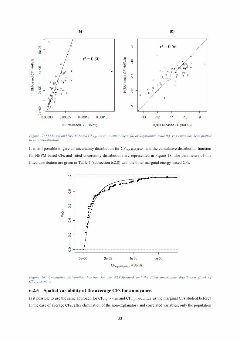
53

Figure 17: SM-based and NEPM-based CFmgn,HAP,HGV,J with a linear (a) or logarithmic scale (b). y=x curve has been plotted

to ease visualisation.

It is still possible to give an uncertainty distribution for CFmgn,HAP,HGV,J and the cumulative distribution function

for NEPM-based CFs and fitted uncertainty distributions are represented in Figure 18. The parameters of this

fitted distribution are given in Table 7 (subsection 6.2.8) with the other marginal energy-based CFs.

Figure 18: Cumulative distribution function for the NEPM-based and the fitted uncertainty distribution (line) of

CFmgn,HAP,HGV,J.

6.2.5 Spatial variability of the average CFs for annoyance.

Is it possible to use the same approach for CFavg,HAP,IRIS and CFavg,HAP,extended as the marginal CFs studied before?

In the case of average CFs, after elimination of the non-explanatory and correlated variables, only the population

r² = 0.56

r² = 0.30

54

density and the sound energy density in the area of calculation should be considered. An SM is thus established

for CFavg,HAP,IRIS using dpop,IRIS and dJ,IRIS, and another is established for CFavg,HAP,extended using dpop,extended and

dJ,extended, where extended refers to the area containing both the IRIS and its internal buffer (Figure 8).

For CFavg,HAP,IRIS, the SM (40) has been obtained with a fitted r² of 0.94 while using lm on the logarithm of the

output CF and the input variables. The r² between the NEPM-based CFs and SM-based CFs is 0.90. NEPM-based

and SM-based CFs are presented in Figure 19. The SM for CFavg,HAP,IRIS give results very close to the one

calculated with the noise prediction software and associated acoustic models.

, ��, = . − ∗ ,.,.

(40)

Figure 19: SM-based and NEPM-based CFavg,HAP,IRIS with a linear (a) or logarithmic scale (b).y=x curve has been plotted to

ease visualisation.

For CFavg,HAP,extended, the SM (41) has been obtained with a fitted R² of 0.99 (Figure 20). For the correlation between

NEPM-based and SM-based CFs, an r² of 0.98 was found. To be able to predict the results with this degree of

accuracy with only two variables is notable (Figure 20), especially since no propagation model is needed to access

these two variables, only an emission model to calculate the sound energy density from the traffic.

, ��, = . − ∗ ,.,. (41)

r² = 0.94 r² = 0.90

55

Figure 20: SM-based and NEPM-based CFavg,HAP,extended with a linear (a) or logarithmic scale (b).y=x curve has been plotted

to ease visualisation.

SMs for CFavg,HAP,IRIS (40) and CFavg,HAP,extended (41) show significant differences when looking at the power of the

population density and the sound energy density. To understand what these differences could imply, CFavg,HAP,IRIS

was predicted using (41) for dpop,IRIS and dJ,IRIS. CFavg,HAP,extended was predicted using (40) for dpop,extended and

dJ,extended. The results are displayed in Figure 21.

For both CFs, changing the SM used leads to some deviation, as one can see by comparing Figure 21 to Figure

20 or Figure 19. However, considering the differences between (40) and (41), this deviation is not as high as

expected. Applying (41) instead of (40) for CFavg,HAP,IRIS leads to less deviation than applying (40) instead of (41)

for CFavg,HAP,extended. This suggests that (41) is preferred to model average CFs, and there is a theoretical reason

that also supports this choice. When establishing an SM, the multiple sampling of shared areas between several

IRIS (Figure 9, section 6.1) while calculating CFavg,HAP,extended is not a problem since this model is only here to

predict the output from the inputs. In this case, CFavg,HAP,extended is a better candidate than CFavg,HAP,IRIS since the

wider geographical area on which it is calculated ensures lower border effects and thus a more accurate predictive

model. The SM that should be used for average CFs for annoyance is thus the one exposed in (41).

r² = 0.99 r² = 0.98

56

Figure 21: SM-based CFavg,HAP,IRIS obtained with (25) (a and b) and CFavg,HAP,extended obtained with (40) (c and d) plotted

against NEPM-based with a linear (a and c) or logarithmic scale (b and d). y=x curve has been plotted to ease visualisation.

6.2.6 Spatial variability of CFs for sleep disturbance

It is possible to establish SMs model for sleep disturbance CFs with the same approach as the ones developed for

annoyance. The only difference is that the sound energy density must only be calculated over the night period.

The sound energy density calculated over the night period dJnight is the total sound energy emitted during the night

periods over a year divided by the area in which the calculation is done. SMs for CFmgn,HSDP,LV,J, CFmgn,HSDP,HGV,J

and CFavg,HSDP,extended are presented in (42), (43) and (44). The lm function returns, respectively, R² values of 0.82,

0.65 and 0.98, corresponding to an r² 0.75, 0.41 and 0.98 on the real data. SM-based values have been plotted

against NEMP-based ones in Figure 22.

, ��,��, = . − ∗ ,.ℎ ,.

(42)

, ��, �, = . − ∗ ,.ℎ ,.

(43)

r² = 0.97

r² = 0.88

r² = 0.98

r² = 0.94

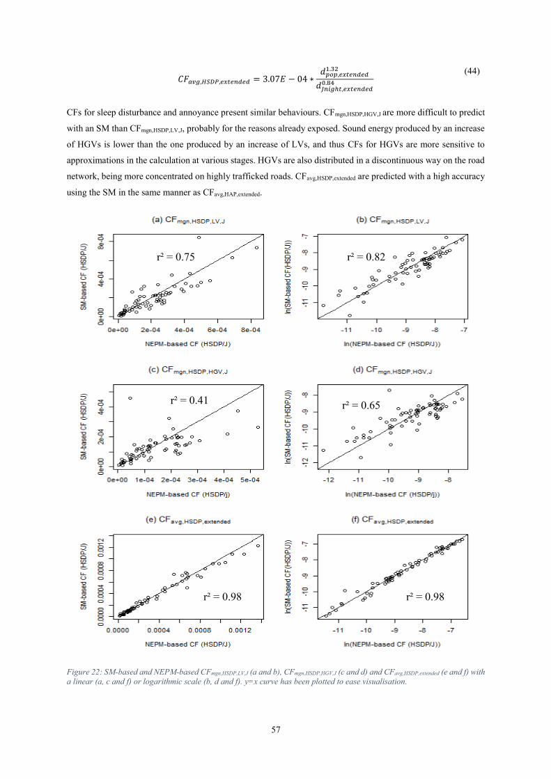
57

, ��, = . − ∗ ,.ℎ ,.

(44)

CFs for sleep disturbance and annoyance present similar behaviours. CFmgn,HSDP,HGV,J are more difficult to predict

with an SM than CFmgn,HSDP,LV,J, probably for the reasons already exposed. Sound energy produced by an increase

of HGVs is lower than the one produced by an increase of LVs, and thus CFs for HGVs are more sensitive to

approximations in the calculation at various stages. HGVs are also distributed in a discontinuous way on the road

network, being more concentrated on highly trafficked roads. CFavg,HSDP,extended are predicted with a high accuracy

using the SM in the same manner as CFavg,HAP,extended.

Figure 22: SM-based and NEPM-based CFmgn,HSDP,LV,J (a and b), CFmgn,HSDP,HGV,J (c and d) and CFavg,HSDP,extended (e and f) with

a linear (a, c and f) or logarithmic scale (b, d and f). y=x curve has been plotted to ease visualisation.

r² = 0.82

r² = 0.65

r² = 0.98

r² = 0.75

r² = 0.41

r² = 0.98

58

6.2.7 Use of these surrogate models and generalisation

SMs have been proposed for marginal and average CFs calculated on a joule basis for the midpoint level. Similar

models will not be proposed for energy-based CFs for two reasons: (1) these CFs are considered less accurate and

(2) aggregating together vkm from LVs and HGVs can lead to significant errors. Similar models for endpoint

levels will not be proposed because they can be obtained from the midpoint levels by multiplying with the

corresponding DW (see subsection 2.1). Similar models for unspecified vehicle types or unspecified time periods

will not be proposed because the practitioner calculating the different input parameters in order to use the SMs

should have access to the repartition of traffic between the different vehicle types and between the different time

periods since it is one of the mandatory parameters for the noise emission model. He can thus, if needed, calculate

more accurate CFs for unspecified vehicles and/or unspecified time periods.

Given the good predictive capacity of this SM, they are judged to be more accurate than weighted mean CFs or

uncertainty distribution if a practitioner wants to estimate CFs in a well-known situation. If a practitioner has

access to GIS data containing all the needed information to apply an emission model but does not have the time

or tools to apply a propagation model, the SMs proposed here to calculate personalised CFs may be a good option

if applied in similar conditions in term of population density and sound energy density. A personalised uncertainty

distribution could also been built by the practitioner, using a lognormal distribution. The mean of this distribution

should coincide with the personalised CF value found and the standard deviation should be estimated by the

practitioner based on its data but should be lower than the one given for the corresponding CFs in the next section

since the geographical situation is well-known.

6.2.8 Use of the uncertainty distributions and evaluation for the whole set of CFs.

As discussed in 6.2.3, an uncertainty distribution of the 67 points available for each IRIS may be the best way to

correctly render the ontic uncertainty of the proposed CFs. Said uncertainty distribution could then be used to

assess the uncertainty due to the spatial variability of the CFs. For an example of how these uncertainty

distributions could be used, please refer to 6.7.2. When plotting the cumulative distribution function of the fitted

distribution and NEPM-based CFs, figures similar to Figure 16 (section 6.2.3) and Figure 18 (section 6.2.4) are

obtained. For example, the case CFävg,HAP,extended is displayed in Figure 23. Uncertainty distributions have been

obtained for all the studied CFs to take into account the spatial variability. The lognormal distribution is the

distribution that better fits our results. The probability density function PDF of the lognormal distribution is given

in (25) where µ is the mean and σ is the standard deviation.

= ∗ � ∗ √ ∗ � ∗ − ln −� ²∗�² (45)

The weighted mean, minimum, maximum and estimates for the lognormal uncertainty distribution will be

presented in tables for all the CFs presented in this work. Table 6 shows all the results for average CFs, Table 7

does the same for the marginal energy-based CFs and Table 8 for the marginal distance-based CFs. CFs for

unspecified vehicle types have not been examined because the vehicle type is considered as known by the

practitioner in most cases. Weighted mean values for the different CFs are analysed and discussed in the next

subsection 6.3.

59

Figure 23: Cumulative distribution function for the NEPM-based CFs and the fitted uncertainty distribution (line) of

CFmgn,HAP,extended.

Table 6: Weighted mean, minimum, maximum and parameters of the lognormal uncertainty distribution fitting for all of the

average CFs calculated in the IRIS or extended area.

Parameters of the lognormal

uncertainty distribution

CFs Weighted

mean

Minimum Maximum Mean µ Standard

deviation σ

CFavg,HAP,IRIS (HAP/J) 2.59E-05 2.82E-06 1.81E-04 -11.10 1.064

CFavg,HSDP,IRIS (HSDP/J) 1.39E-04 1.62E-05 1.70E-03 -9.62 1.186

CFavg,day,IRIS (DALY/J) 5.18E-07 5.64E-08 3.61E-06 -15.01 1.064

CFavg,night,IRIS (DALY/J) 1.01E-05 1.22E-06 1.23E-04 -12.23 1.177

CFavg,uns,IRIS (DALY/J) 1.23E-06 1.50E-07 8.23E-06 -14.121 1.026

CFavg,HAP,extended (HAP/J) 3.30E-05 3.01E-06 1.76E-04 -10.85 1.041

CFavg,HSDP,extended (HSDP/J) 1.71E-04 1.62E-05 1.70E-03 -9.45 1.256

CFavg,day,extended (DALY/J) 6.61E-07 6.02E-08 3.52E-06 -14.76 1.042

CFavg,night,extended (DALY/J) 1.25E-05 8.33E-07 9.92E-05 -12.05 1.242

CFavg,uns,extended (DALY/J) 1.58E-06 1.36E-07 8.52E-06 -13.90 1.051

60

Table 7: Weighted mean, minimum, maximum and parameters of the lognormal uncertainty distribution fitting for all of the

marginal energy-based CFs.

Parameters of the lognormal

uncertainty distribution

CFs Weighted

mean

Minimum Maximum Mean µ Standard

deviation σ

CFmgn,HAP,LV,J (HAP/J) 1.81E-05 2.09E-06 1.16E-04 -11.49 1.104

CFmgn,HAP,HGV,J (HAP/J) 9.89E-06 1.75E-06 1.78E-04 -12.07 1.021

CFmgn,HSDP,LV,J (HSDP/J) 8.58E-05 7.46E-06 8.35E-04 -10.09 1.230

CFmgn,HSDP,HGV,J (HSDP/J) 3.49E-05 5.10E-06 5.28E-04 -10.97 1.177

CFmgn,day,LV,J (DALY/J) 3.62E-07 4.18E-08 2.33E-06 -15.40 1.105

CFmgn,day,HGV,J (DALY/J) 1.98E-07 3.49E-08 3.55E-06 -15.98 1.021

CFmgn,night,LV,J (DALY/J) 6.30E-06 5.64E-07 6.08E-05 -12.69 1.221

CFmgn,night,HGV,J (DALY/J) 2.58E-06 3.92E-07 4.05E-05 -13.55 1.161

CFmgn,uns,LV,J (DALY/J) 7.69E-07 9.13E-08 5.22E-06 -14.65 1.075

CFmgn,uns,HGV,J (DALY/J) 5.74E-07 1.06E-07 6.95E-06 -14.89 0.974

61

Table 8: Weighted mean, minimum, maximum and parameters of the lognormal uncertainty distribution fitting for all of the

marginal distance-based CFs.

Parameters of the lognormal

uncertainty distribution

Weighted mean Minimum Maximum Mean µ Standard

deviation σ

CFmgn,HAP,LV,vkm (HAP/vkm) 1.14E-05 1.86E-06 6.58E-05 -11.76 0.887

CFmgn,HAP,HGV,vkm (HAP/vkm) 5.10E-05 1.27E-05 2.56E-04 -10.24 0.841

CFmgn,HSDP,LV,vkm (HSDP/vkm) 6.06E-05 8.56E-06 4.89E-04 -10.17 0.967

CFmgn,HSDP,HGV,vkm (HSDP/vkm) 2.07E-04 3.87E-05 1.44E-03 -8.93 1.001

CFmgn,day,LV,vkm (HSDP/vkm) 2.28E-07 3.73E-08 1.32E-06 -15.67 0.886

CFmgn,day,HGV,vkm (DALY/vkm) 1.02E-06 2.55E-07 5.13E-06 -14.15 0.841

CFmgn,night,LV,vkm (DALY/vkm) 4.45E-06 6.39E-07 3.55E-05 -12.77 0.962

CFmgn,night,HGV,vkm (DALY/vkm) 1.54E-05 2.97E-06 1.05E-04 -11.52 0.987

CFmgn,uns,LV,vkm (DALY/vkm) 4.85E-07 7.52E-08 2.95E-06 -14.93 0.871

CFmgn,uns,HGV,vkm (DALY/vkm) 2.96E-06 7.75E-07 1.30E-05 -13.08 0.798

6.3 Weighted mean of the CFs over the whole tested sample

In subsection 6.2.2, we failed to find a typology. Moreover, it was shown, based on the calculated CFs in the 67

IRIS, that the weighted mean of CFs is the more representative choice for single values CFs. To calculate the

weighted mean value, the weight of each IRIS corresponds to its level of traffic. This approach reflects the higher

probability to be in an IRIS with heavy traffic. For example, for a marginal CF, CFmgn,HAP,LV,J the weight of each

CF is the number of joules added between scenario (i) and (ii) while increasing LVs.

6.3.1 Average approach

The weighted means of the average CFs were calculated either on the IRIS alone, the internal buffer alone or in

the IRIS and the internal buffer together, referred as extended (see Figure 8 for clarification). An additional CF

has been calculated at the endpoint level for cases where the time period would be unspecified (because

information about the time period is not available in the LCI). For example, CFavg,uns is the weighted mean of

CFavg,day and CFavg,night considering the number of joules emitted during the periods covered by these CFs (46).

, = , ∗ + + , ℎ ∗ ℎ+ + ℎ (46)

62

All of the weighted means for average CFs are presented in Table 9. The midpoint CF for annoyance is valid for

the whole day while the one for sleep disturbance only valid at night. The CFs for the day period are obtained by

multiplying the results in annoyance by the corresponding disability weight, while the CFs for the night period

are the result of both annoyance and sleep disturbance. For the night period, sleep disturbance accounts for 95%

of the result.

Table 9 shows an important difference between the CF for the day and evening and the CF for the night. A joule

of sound energy emitted at night is twenty times more impactful than a joule emitted during the day. This

difference is yet difficult to take into account in the framework of LCA where temporal differentiation at this scale

is uncommon. Environmental noise impact on human health highlights the need for a better temporal

differentiation such as the one proposed in Tiruta-Barna et al. (2016).

Table 9: Weighted mean of CFavg,HAP, CFavg,HSDP, CFavg,day and CFavg,night while calculating them on the IRIS alone, on the

internal buffer alone or extended (both areas taken together).

CF Unit IRIS Internal buffer Extended

CFavg,HAP HAP/J 2.59E-05 3.35E-05 3.30E-05

CFavg,HSDP HDSP/J 1.39E-04 1.74E-04 1.71E-04

CFavg,day DALY/J 5.18E-07 6.71E-07 6.61E-07

CFavg,night DALY/J 1.01E-05 1.28E-05 1.25E-05

CFavg,unspecified DALY/J 1.23E-06 1.60E-06 1.58E-06

The weighted mean of CFavg,uns, is two times higher than CFavg,day and twelve times lower than CFavg,night. CFs for

unspecified time periods are closer to CFs for the day period because there is more traffic during the day than the

night. Not only is the hourly volume of traffic during night lower, but the day period also lasts for sixteen hours

while the night periods only lasts for eight. The ratio between the number of joules during the day period and the

number of joules during the night period is a little bit over 11:1 when looking at the summation over the 67 IRIS.

Table 9 also shows differences in CFs depending on the area in which the average CFs are calculated. The CFs

calculated on the internal buffer are similar to the ones calculated on the extended area, while the CFs calculated

on the IRIS alone are a little bit lower. The proximity between the CFs calculated on the internal buffer alone and

the CFs calculated on the extended area is due to the area of the internal buffer being greater than the area of the

IRIS. The arithmetic mean of the ratio between the area of the internal buffer and the area of the IRIS is 20,

although this ratio ranges from 2 to 72, due to the IRIS not being of a standardised size.

If the whole area was entirely homogeneous in terms of population distribution and road network, the average

CFs would be exactly the same everywhere. The difference between CFs calculated on the IRIS and on the internal

buffer could have two possible origins. Since the IRIS do not have all the same sizes and are not evenly distributed,

this difference can come from the multiple sampling of some areas and not others while calculating CFs on the

extended areas. This was visible earlier in Figure 9, where parts of the internal buffers are shared between multiple

63

calculations. Another origin explaining the difference could come from a possible bias in the sample: selected

IRIS have higher CFavg than their surroundings. However, this possible bias does not seem critical since the CFs

calculated on internal buffer are only 25-30% higher. Considering that IRIS without populations or with only a

few were taken out of the sample, this result is not surprising, so it is more likely that the differences come from

either multiple or missed counting.

The method developed in section 5 has been optimized to be as accurate as possible while calculating marginal

CFs. With marginal CFs, influences of the surroundings are taken into account by applying the road point-of-view

(section 5.2.4). When calculating the average CFs, areas next to the main area of calculation will contribute to the

noise exposure of the area under study (like the internal buffer while calculating the CFs for the IRIS alone).

Along those same lines, traffic in the calculation area will contribute to the noise exposure outside of the area

under study but will be fully allocated to the exposure of the area under study. With the average approach, there

is no way to get away from the influence of the surroundings. Calculating an average CF in an area with heavy

traffic surrounded by inhabited buildings will lead to underestimation, while calculating an average CF in an area

heavily populated surrounded by heavy trafficked roads will lead to an overestimation. The wider the calculation

area, the less these border effects would influence the results. Likewise, CFs calculated on the extended area are

less sensitive to their surroundings, but they are also averaged over a larger area, from 4 km² to 16 km².

To compare average and marginal CFs, it is better to use average CFs calculated on the IRIS alone because the

same geographical area will be considered. To calculate a weighted mean of the average CFs, the ones calculated

on the IRIS alone make the most sense because they are calculated on exclusive geographical areas and thus avoid

multiple sampling. However, if a better estimation of an average CF is needed, using the ones calculated on the

extended area seems to be the best solution since it decreases the influence of the border effect (e.g. it was the

case in subsection 6.2.5). Depending on the context, these two sets of CFs have an interest in LCA, and that is

why both sets of average CFs (those calculated on the IRIS area and on the extended area) will be kept. CFs

calculated on the internal buffer alone do not seem to have any interest, and they will not be further studied.

6.3.2 Marginal approach

The weighted mean of the CFs obtained with a marginal approach are given in Table 10. Since the weightings are

built on the increase between scenario (i) and scenario (ii), the weightings are done on the increase in vkm when

calculating distance-based CFs and on the increase in joules for energy-based CFs. CFs have also been calculated

for unspecified vehicles by weighting the CFs for LVs and HGVs by the percentage of LVs and HGVs in the

traffic of the IRIS. CFs have also been calculated for unspecified time period by weighting the day and the night

periods by the amount of traffic occurring during these periods in a way similar to the one described in (46).

64

Table 10: Distance-based and energy-based CFmgn at midpoint and endpoint levels for LVs, HGVs and unspecified.

CFmgn

Unit

Distance-based Energy-based

LV HGV Unspecified LV HGV Unspecified

per: vkm vkm vkm J J J

CFmgn,HAP HAP 1.14E-05 5.10E-05 1.33E-05 1.81E-05 9.89E-06 1.58E-05

CFmgn,HSDP HSDP 6.06E-05 2.07E-04 7.48E-05 8.58E-05 3.49E-05 6.18E-05

CFmgn,day DALY 2.28E-07 1.02E-06 2.64E-07 3.62E-07 1.98E-07 3.16E-07

CFmgn,night DALY 4.45E-06 1.54E-05 5.54E-06 6.30E-06 2.58E-06 4.61E-06

CFmgn,uns DALY 4.85E-07 2.96E-06 5.99E-07 7.69E-07 5.74E-07 7.14E-07

Table 10 shows a factor of 13-20 between the impact of one joule of sound energy (or one vkm) emitted during

the night and the impact of one joule of sound energy (or one vkm) emitted during the day. This highlights a

significant difference in terms of impact between these two time periods. When looking at the CFs for night, more

than 94% of the impact is coming from sleep disturbance while the CFs for day and evening is only depending on

annoyance. Marginal CFs for an unspecified time period are closer to the ones from the day than to the one for

the night. This is due to the higher road traffic occurring during the day: 95% of the traffic in LVs and 88% of the

traffic in HGVs occur during the day period (between 6 a.m. and 10 p.m.).

Table 10 also shows the difference between CFs for LVs and HGVs. Since an LV is emitting less noise than an

HGV, it is logical to find lower distance-based CFs for LVs. However energy-based CFs are obtained by dividing

human health impacts by the sound energy emitted. By doing so, these CFs are shown to be not sensitive to the

differences in terms of noise emission power levels. The difference between LVs and HGVs on a distance-based

approach comes from difference in the repartition of these two types of vehicles among the road network. HGVs

are often concentrated on heavily trafficked roads further away from a heavily inhabited area. Energy-based CFs

for LVs are 1.5-2.5 times higher than CFs for HGVs. Seeing a visible effect emerge from the different repartition

of LVs and HGVs among the road network is new finding.

Energy sound summed over the 67 IRIS have been divided by the amount of vkm summed over the 67 IRIS to

estimate the mean number of joules per vkm in the studied sample. This operation has been done for the day and

night periods (Table 11). One can see that the number of joules per vkm is higher for night than for day. This

implies that the mean speed during the night period is a little bit higher than the mean speed during the day period

for both vehicle types. The calculation for the unspecified time period uns has been done by summing the EFs

over the whole day (both day and night). Since a large part of the traffic is occurring during the day, the ratio for

unspecified time is closer to the ratio for day than the ratio for night.

65

Table 11: Mean number of joules per vkm calculated from the weighted mean of the marginal CFs.Ratio of CFmgn,__,vkm by

CFmgn,__,J.

LV HGV

, , 0.62 5.03

, ℎ, ℎ 0.70 5.95

, , 0.63 5.16

6.3.3 Comparison between average and marginal approaches

Both approaches are compared at the midpoint for annoyance and sleep disturbance and endpoint level for day,

night and an unspecified time period in Table 12. The weighted means of the average CFs were calculated based

on the IRIS (and not extended). The weighted mean of energy-based marginal CFs were calculated for LVs,

HGVs, and unspecified vehicle type. The unspecified vehicle is a weighted mean of CFs for LV and HGV, the

weights being the respective amount of sound energy. CFs given in Table 12 are the ones already presented in the

two previous subsections.

Table 12: Comparing average and marginal CFs at the midpoint and endpoint level.

Marginal approach Average approach

LV HGV Unspecified

vehicle

LVs and HGVs

Annoyance (HAP/J) 1.81E-05 9.89E-06 1.58E-05 2.59E-05

Sleep disturbance (HSDP/J) 8.58E-05 3.49E-05 6.18E-05 1.39E-04

Day (DALY/J) 3.62E-07 1.98E-07 3.16E-07 5.18E-07

Night (DALY/J) 6.30E-06 2.58E-06 4.61E-06 1.01E-05

Unspecified time (DALY/J) 7.69E-07 5.74E-07 7.14E-07 1.23E-06

Table 12 shows that CFs obtained with the marginal and average approaches are close. Average CFs are less than

two times higher than marginal CFs obtained with unspecified vehicle type. Close values between CFs obtained

with marginal and average approaches imply that the marginal and average CFs are not overly sensitive to the

traffic in the reference situation in which they are calculated. This result validates the point mentioned in 5.2.5

regarding the linear tendency between the numbers of additional HAP and the increased proportions of the studied

traffic. Additionally, considering that CFavg are systematically higher than CFmgn, one can expect higher values

for CFmgn in area with lower traffic than the ones calculated here.

66

6.4 Influence of other sources of uncertainty

Studying the uncertainty of the CFs is important to evaluate their reliability and accuracy. Due to the long

calculation time, software limitations and complexity, the noise propagation software, CadnaA, is considered as

a “black box.” However, it is still possible to roughly study the sensitivity of the results’ potential errors with

simple analyses. To calculate energy-based CFs, two different elements are taken out of CadnaA:

the emission power level of the line sources, i.e. the roads and the associated Lw/m as calculated by a noise

emission model

the highest noise exposure level for each inhabited building, i.e. the exposure of the population after noise

propagation.

Modifying Lw/m or the exposure of the population (Lden in the case of annoyance) allows one to understand the

implications of potential uncertainties in the emission or propagation parts of the calculation. The investigated

output of the model is the weighted mean of CFmgn,day,LV,J.

6.4.1 Influence of a systematic error on noise exposure levels

One of the first things to test is the influence of a systematic error on the noise exposure level. For each evaluated

building, the noise exposure levels are modified by adding a given amount of dB(A) Errexposure,systematic after the

calculation by the noise prediction software, i.e. after calculation of noise emission and propagation. This relates

the influence of a systematic error on the noise exposure level obtained after the propagation in the noise prediction

software. The systematic error was tested with Errexposure,systematic varying between -10 dB(A) and +10 dB(A).

Subtracting 10 dB(A) from the noise exposure levels is equivalent to dividing the sound energy received at the

receptors by a factor ten while adding 10 dB(A) to the noise exposure levels is equivalent to multiply the sound

energy received at the receptors by a factor ten. In other words, a potentially large error is investigated here.

Results are represented in Figure 24 for the weighted mean of CFmgn,day,LV,J.

Figure 24: Influence of a systematic error on the noise exposure levels for the weighted mean of CFmgn,day,LV,J.

67

The minimum value for CFmgn,day,LV,J is 1.59E-07 DALY/J obtained for a systematic error of -10 dB(A) for all the

noise exposure levels; the maximum value is 4.42E-07 DALY/J obtained for + 5dB(A). When varying the sound

energy received at the receptor points by two orders of magnitude, the output is varied by less than a factor of

three; the result is not sensitive to systematic error in the noise exposure levels.

The maximum is reached for an error of +5 dB(A) and not as one could expect at +10 dB(A). This is because the

dose-response relationship for annoyance is only valid between 45 dB(A) and 75 dB(A). A population exposed to

noise levels below 45 dB(A) is not taken into consideration. A population exposed to noise levels above 75 dB(A)

is evaluated at 75 dB(A) for annoyance. While modifying noise exposure levels that have systematic errors,

buildings are taken out of the calculation if a decrease in the noise exposure drops below 45 dB(A) or if an increase

surpasses 75 dB(A) (in the latter case, a change in exposure does not imply a change in the share of HAP in that

building). Increasing all noise exposure levels by more than +5 dB(A) may lead to noise levels surpassing

75 dB(A) for multiple buildings which consequently reduces the weighted mean CFmgn,day,LV,J.

A systematic error can come from the propagation model or the implementation in the noise prediction software.

A wide range for this error, from -10 dB(A) to +10 dB(A) was used, although a systematic error of 10 dB(A) is

unlikely. Mioduszewski et al. (2011) showed that the deviation between the noise prediction model, and the

measurements is not constant. Thus one can ask what would be the influence of a random error on noise exposure

levels on the resulting CF?

6.4.2 Influence of a random error on noise exposure levels

When calculating the weighted average CFmgn,day,LV,J, a random error was considered for each building evaluated

in this study. For each building, the random error follows a uniform uncertainty distribution varying between

– Errexposure,random and + Errexposure,random. While analysing the influence of this parameter, Errexposure,random varied

between 0 dB(A) and +10 dB(A), thereby increasing the width of the uniform distribution from which the random

error is picked for each evaluated building. A maximum value of 3.62E-07 DALY/J is found without any random

error, and a minimum value of 3.41E-07 DALY/J is found while picking a random error in a uniform distribution

ranging from - 10 dB(A) to + 10 dB(A).

Thus, a random error, as long as it is drawn in a symmetrical uncertainty distribution, has little influence on the

output. Negative and positive errors compensate for each other. The slight decrease found while increasing the

width of the uniform distribution in which the random error is picked is probably due to the threshold effect

explained earlier. Adding a random error to the noise exposure levels has a higher chance to push buildings out

of the range in which they have influence than to bring them in.

6.4.3 Influence of a higher error on lower noise exposure levels

Meyer et al. (2017) found that lower noise exposure levels are more sensitive to a change in the search radius dmax.

Since dmax was fixed to 1000 m instead of the preferable choice of 2000 m due to technical constraints (subsection

4.3), it could be interesting to roughly evaluate the possible uncertainties induced by this choice. Fig. 5 in Meyer

et al. (2017) shows the difference in noise exposure levels between calculation with a dmax of 2000 m and

calculation with a dmax of 1000 m. To maximize the error coming from this difference, an amount of dB(A) has

68

been added to noise exposure levels following (47) giving a correction of +10 dB(A) for a noise exposure level

of 45 dB(A) and a correction of 0 dB(A) for noise exposure level of 75 dB(A)

� � = − �

(47)

The weighted mean of CFmgn,day,LV,J with this error is 4.87E-07, 35% higher than the reference value. However,

this correction is an overestimation of the potential difference of changing dmax since it is based on the maximum

difference possible in the worst situation. If all the calculations were rerun with a dmax of 2000 m, the deviation

would be lower than 35%. Considering the significance of the correction, a change of 35% is not substantial. Since

we are looking at a marginal factor, the effect of the correction is due to the shape of the dose-response relationship

(Miedema and Vos, 2007). The weighted mean of CFmgn,day,LV,J increases with an increase in the different noise

exposure levels because the derivative of the dose-response relationship is positive.

6.4.4 Influence of an error on the noise emission level

Since the emission noise levels are also taken out of the noise prediction software for the normalization in joules,

the influence of an error of these noise emission levels can also be investigated. The Figure 2.2 of the SETRA

Copyright (Collective) (2009a) show the variability of the roads measured during the measurement campaigns

used to produce the noise emission model. Based on this figure, an error was added to Lw: Erremission,systematic varying

between -3 dB(A) and +3 dB(A). It is unlikely that the same error was made for all roads while calculating Lw,

the only goal of this calculation is to give an estimation of the sensitivity of the resulting weighted mean

CFmgn,day,LV,J towards the possible sources of uncertainties.

While varying the error on the noise emission level the resulting weighted mean CFmgn,day,LV,J, shown in Figure

25, evolves proportionally to the relative change in terms of sound energy. An error of +3 dB(A) implies a

doubling of the noise emission power and thus a doubling of the sound energy. Since this amount of sound energy

is used to normalize the CFs, the weighted mean CFmgn,day,LV,J is halved. For the same reason, applying -3 dB(A)

halves the resulting sound energy and doubles the weighted mean CFmgn,day,LV,J. The resulting CF is thus sensitive

to this parameter. However, if one tests the effect of a random error for each road picked in a symmetrical

uncertainty distribution, one would probably find a lower effect.

69

Figure 25: Influence of a systematic error on the sound emission levels for the weighted mean of CFmgn,day,LV,J.

A change in the noise emissions should also affect the resulting exposure levels. Varying both Lw and Lden by the

same amount yields different results (Figure 26). Since the CF increases with an increase of exposure and

decreases with an increase of noise emission level, combining the two leads to a slightly smaller variation. The

resulting CF is still sensitive to normalization, i.e. to an error in Lw, but less sensitive to errors in the propagation

part.

Figure 26: Influence of a systematic error on both the sound emission level Lw and the noise exposure level Lden for the weighted

mean of CFmgn,day,LV,J.

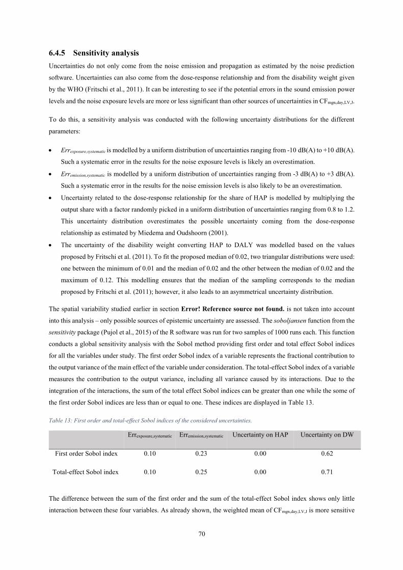
70

6.4.5 Sensitivity analysis

Uncertainties do not only come from the noise emission and propagation as estimated by the noise prediction

software. Uncertainties can also come from the dose-response relationship and from the disability weight given

by the WHO (Fritschi et al., 2011). It can be interesting to see if the potential errors in the sound emission power

levels and the noise exposure levels are more or less significant than other sources of uncertainties in CFmgn,day,LV,J.

To do this, a sensitivity analysis was conducted with the following uncertainty distributions for the different

parameters:

Errexposure,systematic is modelled by a uniform distribution of uncertainties ranging from -10 dB(A) to +10 dB(A).

Such a systematic error in the results for the noise exposure levels is likely an overestimation.

Erremission,systematic is modelled by a uniform distribution of uncertainties ranging from -3 dB(A) to +3 dB(A).

Such a systematic error in the results for the noise emission levels is also likely to be an overestimation.

Uncertainty related to the dose-response relationship for the share of HAP is modelled by multiplying the

output share with a factor randomly picked in a uniform distribution of uncertainties ranging from 0.8 to 1.2.

This uncertainty distribution overestimates the possible uncertainty coming from the dose-response

relationship as estimated by Miedema and Oudshoorn (2001).

The uncertainty of the disability weight converting HAP to DALY was modelled based on the values

proposed by Fritschi et al. (2011). To fit the proposed median of 0.02, two triangular distributions were used:

one between the minimum of 0.01 and the median of 0.02 and the other between the median of 0.02 and the

maximum of 0.12. This modelling ensures that the median of the sampling corresponds to the median

proposed by Fritschi et al. (2011); however, it also leads to an asymmetrical uncertainty distribution.

The spatial variability studied earlier in section Error! Reference source not found. is not taken into account

into this analysis – only possible sources of epistemic uncertainty are assessed. The soboljansen function from the

sensitivity package (Pujol et al., 2015) of the R software was run for two samples of 1000 runs each. This function

conducts a global sensitivity analysis with the Sobol method providing first order and total effect Sobol indices

for all the variables under study. The first order Sobol index of a variable represents the fractional contribution to

the output variance of the main effect of the variable under consideration. The total-effect Sobol index of a variable

measures the contribution to the output variance, including all variance caused by its interactions. Due to the

integration of the interactions, the sum of the total effect Sobol indices can be greater than one while the some of

the first order Sobol indices are less than or equal to one. These indices are displayed in Table 13.

Table 13: First order and total-effect Sobol indices of the considered uncertainties.

Errexposure,systematic Erremission,systematic Uncertainty on HAP Uncertainty on DW

First order Sobol index 0.10 0.23 0.00 0.62

Total-effect Sobol index 0.10 0.25 0.00 0.71

The difference between the sum of the first order and the sum of the total-effect Sobol index shows only little

interaction between these four variables. As already shown, the weighted mean of CFmgn,day,LV,J is more sensitive

71

to a systematic error in emission than to a systematic error in population exposure. The Sobol indices are higher

for error on the emission even with a narrower uncertainty distribution for Erremission,systematic than for

Errexposure,systematic. Uncertainty related to DW has a larger influence than other sources of uncertainties. Meyer

et al. (2016) found similar results when conducting sensitivity analyses for other methods that integrate

environmental noise impact in LCA. Since the HAP midpoint indicator is multiplied by DW for annoyance to

obtain the endpoint in DALY for the day period, DW is responsible for a large part of the uncertainty of the result.

Sensitivity analysis is dependent on the uncertainty distribution modelled for each variable, and since the approach

of this subsection is qualitative, results should be used with care. This first approach could be refined with a more

complete modelling of the uncertainties in both the emission and propagation steps.

6.4.6 Influence of other sources of uncertainty for an average CF, CFavg,day,IRIS

To do a similar analysis for every CF proposed in this work would be too time consuming, but it is important to

see for an average CF. Average CFs are expected to behave differently than marginal CFs. Some of the errors

incurred by the average CF could be avoided by using a marginal CF since it is calculated from a change in the

situation. If an error is the same in the reference and increased traffic situations, these errors nullify each other.

An average CF will not reduce of this type of error since it is only calculated from the reference situation. To

highlight this, an analysis of CFavg,day,IRIS will be conducted.

Influence of a systematic error on noise exposure levels

Errexposure,systematic was varied between -10 dB(A) and +10 dB(A) to obtain Figure 27. The variation of the weighed

mean of CFavg,day,IRIS while adding a systematic error on the population exposure presents a different behaviour

than the one presented in Figure 24 for CFmgn,day,LV,J. The weighted mean of CFavg,day,IRIS is 1.88E-07 DALY/J

when the population exposure is decreased by 10 dB(A) and 1.06E-06 DALY/J when the population exposure is

increased by 10 dB(A). The variation between this minimum and maximum is higher than in the case of the

marginal CF; the ratio between the minimum and maximum is 5.6 instead of 2.8. CFavg,day,IRIS is more sensitive to

an error in exposure than CFmgn,day,LV,J. The dose-response for annoyance is a monotonic function, so the average

CF can only increase with the exposure. This accounts for the gradual increase with the change in exposure

contrary to the previous case (subsection 6.4.1) where an increase of exposure led to a decrease of the marginal

CF due to threshold effects.

72

Figure 27: Influence of a systematic error on the noise exposure levels for the weighted mean of CFavg,day,IRIS.

Influence of a random error on noise exposure levels

Adding a random error for the exposure for each building evaluated in this study has minor impact for the weighted

mean of CFavg,day,IRIS similar to the one found for the marginal CF (subsection 6.4.2). The weighted mean of

CFavg,day,IRIS goes from 5.22E-07 DALY/J to 5.71E-07 DALY/J when picking a random error in a uniform

distribution ranging from - 10 dB(A) to + 10 B(A) for every buildings considered.

A random error, as long as it is drawn in a symmetrical uncertainty distribution, has little influence on the output

due to negative and positive errors compensating themselves. The slight increase that was found while increasing

the width of the uniform distribution in which the random error is picked is due to the positive derivative of the

dose-response relationship and to the fact that the threshold effects observed with the marginal CF does not apply

to average CFs.

Influence of a higher error on lower noise exposure levels

To study the influence of a higher error on lower noise exposure levels, the same approach described in section

6.4.3 was applied. To simulate the possible influence of the search radius dmax, an amount of dB(A) was added to

the noise exposure; this gave a correction of +10 dB(A) for a noise exposure level of 45 dB(A) and a correction

of 0 dB(A) for noise exposure level of 75 dB(A), as shown in (25). The resulting weighted mean of CFavg,day,IRIS

with this potential error is 7.39E-07 DALY/J, 42% higher than the reference value. The influence of a higher error

on lower noise exposure levels is slightly higher for the average CF than for the marginal one. However, this

correction is an overestimation of the potential influence of a change in dmax. Considering the importance of the

correction, the induced change is not that high. This result is similar to the one obtained for CFmgn,day,LV,J.

73

Influence of an error on the noise emission level

When looking at the influence of an error on the noise emission level alone, the effect is exactly the same between

average and marginal CFs because, in both cases, the amount of DALY is divided by the amount of joules. Thus,

multiplying or dividing this amount of joules will divide or multiply the resulting CFs in the same proportion.

Varying both the noise emission level Lw and the population exposure Lden by the same amount yields the results

presented in Figure 28. The weighed mean of CFavg,day,IRIS is still sensitive to the normalization part, i.e. to an error

in Lw. When applying -3dB(A) for both emission power levels and population exposure levels, a value of 7.90E-

07 DALY/J is found, while 3.39E-07 DALY/J is found for a change of +3dB(A). When dividing the sound

emission power and the acoustical power at which population are exposed by a factor of four, the weighted mean

of CFavg,day,IRIS is multiplied by 2.3. This is slightly lower than the ratio of 2.7 that could be found for the weighted

mean of CFmgn,day,LV,J (Figure 26). The slightly lower sensitivity of the weighted mean of CFavg,day,IRIS compared to

the weighted mean of CFmgn,day,LV,J, while modifying the noise emission level and the population exposure

simultaneously, comes from the higher sensitivity of the average CF to an error on the population exposure. A

decrease in noise emission levels increase the average CF, while a decrease in population exposure levels decrease

the CF. Since the weighted mean of CFavg,day,IRIS is more sensitive than the weighted mean of CFmgn,day,LV,J to a

change in the population exposure, it compensates for the change in noise emission levels for the average CF a

little more than for the marginal one.

Figure 28: Influence of a systematic error on both the sound emission level Lw and the noise exposure level Lden for the

weighted mean of CFavg,day,IRIS.

Sensitivity analysis

A sensitivity analysis was conducted using the same variables and uncertainty distributions as the one described

in section 6.4.5. The results are displayed in Table 14.

74

Table 14: First order and total-effect Sobol indices of the considered uncertainties.

Errexposure,systematic Erremission,systematic Uncertainty on HAP Uncertainty on DW

First order Sobol index 0.28 0.21 0.01 0.46

Total-effect Sobol index 0.33 0.22 0.02 0.68

Compared to the sensitivity analysis conducted on the weighted mean of CFmgn,day,LV,J in subsection 6.4.5, the

weighted mean of CFavg,day,IRIS is more sensitive to an error in noise exposure levels. This result validates the

assessment made earlier in this subsection where the higher sensitivity of the weighted mean of CFavg,day,IRIS was

highlighted compared to the weighted mean of CFmgn,day,LV,J. This difference decreases the importance of the

uncertainty of the DW mechanically, leading to lower Sobol index values for the average CF than for the marginal

one. Uncertainties related to DW are still responsible for a large part of the resulting CF uncertainties.

The sensitivity analyses conducted in this whole subsection must be cautiously considered because the uncertainty

distributions on which they rely were not accurately quantified. To get an accurate quantification of these

uncertainties, comparing the values found by the noise prediction software with measurements in the field may

be needed. Moreover, due to both temporal and technical constraints, it was not possible to separately assess the

influence of each input of CadnaA, such as the influence of a change in traffic, a change in the average speed, a

change in the distribution of the traffic between LVs and HGVs, etc.. However, the multiple experiments

conducted in different situations have already given an understanding of the variability what a change in all these

parameters could imply. If epistemic sources of uncertainty (uncertainty coming from approximations in the

models/software, from the DW, etc.) were correctly assessed, it would have been possible to include them in the

uncertainty quantification given in section 6.2.8, which only considers the spatial variability observed in the

calculated CFs.

It was also possible to show that average CFs are more sensitive to exposure errors than marginal CFs. This higher

sensitivity to exposure errors leads to a slightly lower sensitivity to emission errors. This subsection also highlights

the importance of the uncertainties coming from the DW compared to other possible sources of epistemic

uncertainty.

6.5 Comparison to previous literature

Comparing the results obtained with existing results from the literature allows one to detect potential errors and

to evaluate the reliability and representativeness of its finding. To be in the same order of magnitude with the

numbers found in literature is not a justification by itself, but inexplicable differences are a good indication of

something amiss. Thus, a literature comparison is a way to ensure avoidable mistakes, especially since other

approaches may not use the same data, the same geographical area and the same software.

6.5.1 Environmental noise impacts on human health

Before comparing the result with existing CFs in the LCA literature, it can be interesting to compare the human

health impacts with the one calculated by Fritschi et al. (2011). In this study, summing over all 67 experiments,

2.19E+04 HAP and 9.67E+03 HSDP were found for the entire studied population. Converting these amounts in

75

DALY (by multiplying with the corresponding DWs, subsection 2.1) and dividing by the concerned population,

2.49E-03 DALY/person was found for annoyance and 3.84E-03 DALY/person for sleep disturbance.

Using the numbers found in Fritschi et al. (2011) for 285 million of European living in cities of more than 50,000

inhabitants, 487,448 DALY were found for annoyance and 800,023 DALY for sleep disturbance. This

corresponds to an impact of 1.17E-03 DALY/person and 2.81E-0.3 DALY/person, respectively. Their estimation

of the burden of disease due to environmental noise was done on an extrapolation of available noise exposure for

cities of more than 250,000 inhabitants.

It is possible to do the same calculation with the available data collected by the European Environment Agency

in the framework of Directive 2002/49/EC (“Reported data on noise exposure covered by Directive 2002/49/EC,”

n.d.). This data covers 117 million citizens living in the European Union and relies on noise assessments produced

by cities for every European country. Using the same method to calculate the burden of disease, 1.98E-03

DALY/person is found for annoyance and 3.32E-03 DALY/person is found for sleep disturbance. These values

are more recent and do not rely on extrapolation, thus making them preferred for comparison.

Compared to the European Environment Agency, the results obtained with the 67 IRIS are 26% higher for the

case of annoyance and 16% higher for the case of sleep disturbance, and they are within the same order of

magnitude. It is difficult to know where these differences are coming from, but it may indicate a slight

overrepresentation of geographical areas with higher impacts in the studied sample. No significant errors or

deviations were found while comparing human health impacts from the studied sample with the existing numbers

calculated at a large scale (European Union).

6.5.2 Distance-based CFs in the LCA literature

The literature is dominated by the distance-based approach when it comes to integrating environmental noise

impacts on human health. Müller-Wenk (2002) already proposed an estimation in DALY for day and night and

for two categories of vehicles more than fifteen years ago. By approximating the Type 1 and Type 2 vehicles from

his study with the LVs and HGVs used in this work, Table 15 is obtained (from Figure 15 in (Müller-Wenk,

2002)).

Table 15: Comparison of the results of Müller-Wenk (2002) and the present work.

(Müller-Wenk, 2002) Present work Müller-Wenk,

CFmgn,day,LV,vkm 1.3 E-07 2.3 E-07 1.8

CFmgn,day,HGV,vkm 1.3 E-06 1.0 E-06 0.77

CFmgn,night,LV,vkm 2.7 E-06 4.5 E-06 1.7

CFmgn,night,HGV,vkm 2.6 E-05 1.6 E-05 0.62

The CFs calculated in this work are in the same order of magnitude as the values found by Müller-Wenk (2002).

This is surprising considering that their CFs were calculated fifteen years ago for the whole of Switzerland using

76

limited data as well as a simpler method compared to the one developed in this work and with different DWs

(Müller-Wenk (2002) used 0.033 for annoyance instead of 0.02 and 0.055 for sleep disturbance instead of 0.07).

In this work, a ratio of 8.1 to 8.5 is found between the mean sound emission power of HGVs and LVs (obtained

by dividing the number of joules per vkm for HGVs by the one for LVs in Table 11, subsection 6.3.2). However,

since HGVs have a lower impact per joule due to a different repartition on the road network, weighted mean CFs

for HGVs are only 3.4 to 5.5 times higher than weighted mean CFs for LVs contrasting with the hypothesis of

Müller-Wenk (2002) of HGVs being 10 times more impactful based on the noise emission levels. Results from

Müller-Wenk (2002) are covered by the minimum-maximum interval found in this work and the difference could

be easily explained by the ontic (e.g. variability) and epistemic (e.g. models and assumptions) uncertainties.

Franco et al. (2010) found 1.3E-3 additional cases of annoyance for an additional 1,000 vkm for vehicles

equivalent to HGVs on Spanish motorways. This leads to 1.3E-06 additional HAP/vkm while the CFmgn,HAP,HGV,vkm

found in this work is 5.10E-05 HAP/vkm. Moliner et al. (2014) found results ranging between 3.88E-08 and

7.63E-08 DALY/vkm for three Spanish motorways considering the addition of one HGV proportional to the

existing annual traffic on the studied road. This corresponds to CFmgn,uns,HGV,vkm, which has a value of 2.96E-06

DALY/vkm. The values found in this work are 40 times higher than the value found by Franco et al. (2010) and

39-76 times higher than the values found by Moliner et al. (2014). Moreover, the values found by Moliner et al.

(2014) and Franco et al. (2010) are lower than the minimal value found in this work for the corresponding CF.

However, most of the CFs from this work were calculated in an urban and suburban context while Moliner et al.

(2014) and Franco et al. (2010) applied their methodology on Spanish motorways. The motorways considered by

Moliner et al. (2014) and Franco et al. (2010) are areas with lower population densities and higher sound energy

densities, thus lower CFs if the SMs hold true (subsections 6.2.3 to 6.2.6). Motorways may be the situation

presenting the lowest CFs.

The LCIA methodology Swiss eco-factors 2013 (Frischknecht and Büsser Knöpfel, 2013) already provides CFs

to integrate environmental noise impact in LCA. They use an average approach to determine the HAP per total

vkm over a given year. By doing this, the vkm of people and freight (considered equivalent to the LVs and HGVs

used in this method) have to be aggregated together. LVs and HGVs have different emission power levels, so to

solve this, Frischknecht and Büsser Knöpfel (2005) multiplied the number of freight (HGVs) by 10. Considering

that freight emits ten times more sound energy (10 dB higher in terms of), this assumption could have been used

to produce average distance-based CFs. However, since the aggregation between LVs and HGVs is done on a

sound energy logic, it has been preferred to only do it, in our work, on an exact quantification of the sound energy

produced (relying on the emission model (SETRA Copyright (Collective), 2009a)). And, as detailed above, this

work does not confirm a ratio of 10 between the impact of LVs and HGVs (subsection 6.3).

Frischknecht and Büsser Knöpfel (2005) found 6.25E-06 HAP/vkm for LVs and 6.25E-05 HAP/vkm for HGVs.

Applying the same methodology to the studied sample leads to 2.47E-06 HAP/vkm and 2.47E-05 HAP/vkm.

Using their method for the studied sample led to the same order of magnitude in the result. It should be noted that

Frischknecht and Büsser Knöpfel (2013) used annoyance as a midpoint (HAP) and proposed separate CFs for

road traffic, rail traffic and air traffic. Different noise sources are only aggregated at the midpoint level and not

earlier at the noise emission level.

77

The environmental priority strategies (EPS) LCIA method (Steen, 1999a, 1999b) uses an approach too different

to allow for comparisons. Impacts from environmental noise were estimated by considering 25% of the global

population is exposed to noise levels above 65 dB(A). They then assumed that the amount of nuisance mainly

occurred during rush hours, which comprises a sixth of the day, and this was divided by an estimate of the total

mileage of the world fleet based on numbers from 1990. This CF does not seem reliable due to the numerous

questionable assumptions on which it is built.

6.5.3 The specific case of Cucurachi

The results obtained by Meyer et al. (2016) at the endpoint level using the CFs and conversion factor proposed by

Cucurachi et Heijungs (2014) were criticized. At the endpoint level, the results from Cucurachi et Heijungs (2014)

were 100,000,000 times higher than the ones obtained with the approach from Franco et al. (2010). However,

Cucurachi et Heijungs (2014) warn about the use of potentially malfunctioning conversion factor between

midpoint and endpoint: “The assumption of linearity allowed for the quantification of a conversion factor, but

may introduce uncertainty that needs to be further investigated into the calculations.”. Thus, the method

developed by Cucurachi and his co-authors (Cucurachi et al., 2012; Cucurachi and Heijungs, 2014) could still

lead to a correct calculation at the midpoint level even if theoretical arguments could be opposed to this midpoint

indicator, such as the aggregation of the emission levels of different noise source types. However, with the data

used in this work and the results obtained, CFs similar to the one proposed by Cucurachi and Heijungs (2014)

could be calculated. The CFs from their work are given in person*Pa/W where person*Pa can be interpreted as

“the number of people that are exposed to a certain sound pressure” (Cucurachi et al., 2012). These CFs are

calculated by assessing the marginal change of person-Pa for a marginal change in the acoustical power in which

the studied population is exposed. This is a marginal approach that considers the background noise existing prior

to the change.

In the data used for this work, the Lday, Levening, Lnight and Lden are available for each inhabited building with the

associated number of persons. Assuming that the sound pressure is constant over each time period (day, evening

and night), these levels can be converted into a long term average sound pressure pt, using (48), that can be

deducted from (6). p0 is the reference pressure (equal to 2*10-5 Pa) (ISO 3744, 2010), t refers to the time period

(t = {day,evening,night}) and βt is the weighting of the periods as used by Cucurahi et al. (2012) (βday=0, βevening=5,

βnight=10).

= √ ∗ ��+�� = ∗ ��+��

(48)

Considering these pressures before pt and after pt’ an increase in traffic of vehicle type j converted in sound

emission power ∆Wt,J, similar CFs to the one from Cucurahi et al. (2012) can be calculated by (49). i refers to a

building.

ℎ , , = ∑ , ,′ − , ∗∆� , (49)

The results from calculating this over the different time periods and using a weighted mean for the sample of 67

different geographical areas are presented in Table 16.

78

Table 16: CFs calculated with the approach proposed by Cucurachi and CFsgiven by Cucurachi and Heijungs (2014).

CFs calculated with the Cucurachi

approach on our data (person*Pa/W)

CFs from Cucurachi and Heijungs (2014)

(person*Pa/W)

Time period LV HGV Urban Suburban Rural Industrial

Day 103 58 4.48E+05 5.63E+05 2.04E+04 1.00E+05

Evening 199 91 8.42E+05 1.01E+06 3.66E+04 1.68E+05

Night 930 466 1.43E+06 1.79E+06 6.49E+04 3.16E+05

Despite using accurate data coming from noise prediction software, we were unable to reproduce the results found

by Cucurachi and Heijungs (2014). The CFs calculated with the method developed by Cucurachi et al. (2012) are

at least 70 times higher (the minimum is found with the CF for rural archetypes during the night period). However,

urban and suburban archetypes are dominating the studied sample and thus the difference is even higher (a factor

around 400). Interpretation of these results are difficult because of the chosen midpoint: what does person*Pa/W

represent? These CFs represent the change in exposure to an acoustical pressure normalised by the change in

sound emission power producing it. In our experiments, the population is fixed over the different time periods, so

this parameter is fixed.

Data gathered to establish CFs do not validate the CFs found by Cucurachi and Heijungs (2014) but rather seem

to highlight errors in the orders of magnitude of these CFs. Finding errors at the midpoint level could, partly,

explain the high results found in Meyer et al. (2016) for the Cucurachi method where the difference in errors was

of eight orders of magnitude. Beyond the quantitative critique of the methods developed by Cucurachi et al.

(2012), there are also theoretical critiques; these will be discussed in section 7.1.

6.6 Connecting to the inventory

For a best use of the CFs developed here, the link between these CFs and the existing LCI processes have to be

detailed. This link will be different if one wants to use the distance-based or energy-based CFs.

6.6.1 Reference vehicle used

A more accurate description of the vehicles used in the noise prediction software is needed. As stated before, the

noise prediction software only have two vehicles of reference: LV and HGV. These reference vehicles have been

built to be representative of the mean vehicle for each category. Lw is calculated in the noise prediction software

used throughout this work following the SETRA Copyright (Collective) (2009a) methods, in particular Table

D.12, D.13, D.14 and D.17. In the data used for this work, all the roads have a surfacing category R2 and an age

of seven years. Without extensive knowledge of said roads, it is not possible to judge the validity of this aspect.

6.6.2 New elementary flows

Most of the road transportation processes in the LCI do not take into account the temporal occurrence of the

operation (e.g. day and night). These processes can then only give an output in an EF where the temporal

79

dimension is unspecified. Given the important difference between the day and night periods, it is advised to take

into account the temporal occurrence of the transportation if possible. To do so, each road transportation process

should be subdivided into day, night and unspecified.

Distance-based

An EF is defined as the material or energy entering the system being studied that has been drawn from the

environment without previous human transformation, or material or energy leaving the system being studied that

is released into the environment without subsequent human transformation (ISO 14040, 2006). As such, an EF in

vkm is not covered by this definition, even if this unit is used as a proxy for sound energy and its impact. However,

several non-material emissions EFs already exist in some LCIA methods (Frischknecht and Büsser Knöpfel,

2013), and the proposed EFs can be added into this category.

LVs and HGVs should be considered separately because there is not only a large difference between these two

vehicle categories on the distance-based CFs but also they are, in most cases, separated in the LCI. Ideally, six

EFs should be created, as shown in Table 17.

Table 17: New elementary flows for distance-based CFs.

Period LVs HGVs

Day Noise, light vehicles, day Noise, heavy goods vehicles, day

Night Noise, light vehicles, night Noise, heavy goods vehicles, night

Unspecified Noise, light vehicles, unspecified Noise, heavy goods vehicles, unspecified

Energy-based

To use the energy-based CFs, several additional EFs have to be created. This time, these EFs are expressed in

joule. These flows would be the same as in Table 17, but the unit would be joule. The differentiation between LVs

and HGVs does not come from the difference in terms of noise emission level, since the energy-based approach

is normalised by the emitted sound energy. The difference stems from the change in distribution over the road

network for these two vehicle types. CFs for HGVs are more representative of freight, while CFs for LVs are

more representative of light vehicles, i.e. passenger transportation.

6.6.3 Calculating the output of the processes

For each existing road transportation process that considers the noise impact on human health, an output to the

corresponding EF has to be created. Using the EFs for LVs or HGVs would depend on the weight of the vehicle

under consideration. A vehicle is considered an LV if the gross vehicle weight rating is under 3.5 tons and an

HGV if it is larger than or equal to 3.5 tons (SETRA Copyright (Collective), 2009a). This broader typology can

be refined to better cover the whole spectra of possible road transportation vehicles.

80

Distance-based

If one wants to consider the difference between the vehicle under consideration and the one used as reference,

Frischknecht and Büsser Knöpfel (2013) proposed factors in Tab. 113 based on the difference in the noise

emission level. For example, if a vehicle under consideration is 5 dB(A) higher than the reference vehicle, the

factor provided is 3.16. Said factors will be applied to the output EF of select transportation processes to take into

account the difference in terms of average noise emission levels between the considered vehicle and the reference

one used to develop the distance-based CFs. However, if a practitioner wants to adapt environmental noise impacts

for vehicles more or less noisy than the reference ones used for LVs and HGVs, it is advised to take the energy-

based approach described hereafter.

Energy-based

The energy-based approach allows for a more refined quantification on the sound emission, since sound emission

power per vkm is not constant. Thus, energy-based CFs are more reliable. And average CFs have been calculated

only using an energy-based approach. This approach allows for a better differentiation of the road transportation

processes. To integrate environmental noise impacts using an energy-based approach, a road transportation

process should have an output EF in joules. If the vehicle under considerations is not well known, one way to use

this approach is to use the number of joules per vkm, as detailed in Table 11. However, this will have the same

benefits and limitations as the distance-based approach.

To have a more detailed differentiation of the inventory processes, the sound emission power level of the vehicle

under consideration should be well known. If the sound emission power level is entirely defined on travel, the

sound energy produced can be precisely calculated and then multiplied by the corresponding CFs. Although, a

more common case would be to have access to a noise emission model for the vehicle under consideration. In that

case, the sound emission power level is dependent upon the speed, road surface, road gradient, etc. Road gradient,

impact of traffic lights or other road infrastructures on the traffic fluidity and other aspects were not considered in

the application of the method but these aspects may be considered in the chosen noise emission model (SETRA

Copyright (Collective), 2009a) or in others. If road parameters are unknown, it is advised to use the same ones

used in the data from which the CFs were produced (i.e. an R2 road surface built seven years ago). The question

remains, what speed should be used to obtain the amount of joules per vkm? From Table 11 (section 6.3.3)

displaying the mean number of joules per vkm, a mean speed can be deduced using the SETRA Copyright

(Collective) (2009a) noise emission model and is displayed in Table 18.

Practitioners elaborating EF outputs for road transportation processes can use this table. For example, for Sound

energy, light vehicles, day, the sound emission power should be calculated for a speed of 67 km/h. If the vehicle

under study is driven in specific conditions, for example only in city centres at a mean speed of 50 km/h, it is

advised to calculate sound energy emitted per vkm under these specific conditions. This is of particular importance

since the uncertainty and sensitivity analyses underlined the importance of the noise emission modelling part

towards the reliability of the result.

81

Table 18: Mean speed in km/h of LVs and HGVs for the weighted mean of marginal CFs.

Mean speed (km/h) LV HGV

Day 66 65

Night 70 72

Unspecified 66 66

6.7 Practical use of the CFs

6.7.1 In existing road transportation processes

Examining an existing LCA process provides an idea of the order of magnitude of the different sources of human

health damage, and one can compare this with human health damage due to environmental noise. For example,

the obtained human health impacts unrelated to noise are displayed in Table 19 for one vkm when looking at the

Transport, passenger car, medium size, petrol, EURO 5 process from the ecoinvent version 3 database (Wernet

et al., 2016) and using the method ReCiPe Endpoint (H) (Goedkoop et al., 2009).

Table 19: Human health impacts for one vkm.

Impact Category Unit Amount

Climate change Human Health DALY 3.43E-07

Ozone depletion DALY 1.15E-10

Human toxicity DALY 1.07E-08

Photochemical oxidant formation DALY 1.48E-11

Particulate matter formation DALY 3.43E-08

Ionising radiation DALY 2.69E-10

Total DALY 3.88E-07

To include noise impacts among the other impacts, the road transportation process under consideration should

have an additional EF (emission occurring in the use phase). The process under consideration would have an

output of one vkm to Noise, light vehicles, unspecified (if using a distance-based approach). If the CFs developed

in this work to assess environmental noise impact on human health are included in the LCIA method used, the CF

corresponding to the EF is used. Thus, the EF Noise, light vehicles, unspecified is multiplied by CFmgn,uns,LV,vkm,

resulting in 4.85E-07 DALY. If the noise impact is integrated with the other human health impacts over the

vehicle’s life cycle, it accounts for 56% of the total amount of DALY produced. Using the maximum value for

CFmgn,uns,LV,vkm leads to noise impact being responsible of 88% of the total impact on human health while using

minimum value leads to 16%. The noise impact is in the same order of magnitude as all the other human health

impacts, thus the contribution of noise among other impact categories is sensitive to errors and uncertainties.

82

This result is consistent with what is found in comparable literature. Most of the existing studies found a

substantial human health damage from noise compared to other sources and are in the same order of magnitude.

Moliner et al. (2013) found 2.5% to 5% noise impact among the total human health while looking at the health

impacts caused by an additional vkm on three Spanish motorways. The values of Moliner et al. (2013) are the

lowest in the literature and is likely due to the analysis being limited to motorways.

If the results found in this work are representative of the overall road transportation, including noise impacts on

human health would double the human health impact of this road transportation process. Noise is far from being

negligible, despite being still a marginal research question in LCA.

Considering a diesel instead of petrol vehicle, like Transport, passenger car, medium size, diesel, EURO 5,

produces a slightly higher noise contribution since the total human health damage is lower for diesel rather than

petrol vehicles (3.62E-07 DALY instead of 3.88E-07 DALY, respectively). A comprehensive assessment of every

road transportation process in the datasets would require the use of noise emission models and data for each

concerned vehicle type to establish EFs in terms of sound energy. This work has not been done during this PhD

thesis due to time constraints.

6.7.2 In the foreground

The CFs developed in this work were applied to the case study developed before (Meyer et al., 2016) with the

goal to evaluate environmental noise impacts of two different tires and to compare it with other impact categories.

Assessing the noise impact of tires is only possible using energy-based CFs since the two tires are differentiated

by their noise emission power.

The emitted sound energy is calculated with the same approach as the one developed to apply the Cucurachi

method (section 2.3 of (Meyer et al., 2016)). A noise emission model (SETRA Copyright (Collective), 2009a) is

used to calculate the sound energy emitted by one vehicle rolling one vkm. This vkm is distributed on the road

network in proportion to the existing traffic among three different road types (motorways, non-urban roads, urban

roads) and three time periods (day, evening and night). Sound energy emissions occurring during the day and the

evening are multiplied by CFmgn,day,LV,J and emissions occurring during the night are multiplied by CFmgn,night,LV,J.

Human health impacts from environmental noise for one vkm of Tire 1 results in 1.59E-07 DALY. Applying the

method proposed by Franco et al. (2010) for the same tire led to 5.00E-08 DALY (Meyer et al., 2016); however,

only annoyance was taken into account by Franco et al. (2010). When only considering HAP, similar results are

obtained: 7.33E-08 DALY. This result is interesting because, for the practitioner, the Franco method is more

complicated (section 2.2 of (Meyer et al., 2016)) than simply using a noise emission model and multiplying the

resulting sound energy by the CFs developed in this work. Finding similar results validates the hypothesis

proposed in section 6.6.2: the difference between the values found in this work and the ones found by Franco et

al. (2010) is coming from the assessment of different situations. Attaining similar results highlights the practicality

of the CFs and the reliability of the results compared to the one obtained with existing method. As a result, the

83

CFs developed in this work seems to be adapted to this case, i.e. representative of the average French network,

even if additional work is needed to support this claim.

The tire case study is also be a good example of how to deal with the uncertainty coming from spatial variability

and taking into account the uncertainty distribution proposed for the different CFs. An uncertainty analysis is

conducted using a Monte-Carlo approach with two samples of 100,000 iterations each. Most of the uncertainty

distributions for the different parameters displayed in Table 20 are the same ones used in Meyer et al. (2016) (see

annex I). CFmgn,HAP,LV,J and CFmgn,HSDP,LV,J were chosen so the uncertainty of the DW can be assessed separately.

The uncertainty distributions for these two CFs are taken from Table 7. Modelling uncertainty distributions for

CFmgn,HAP,LV,J and CFmgn,HSDP,LV,J would be better for a specific location, but doing so for the whole French road

network may be questionable. When looking at an average value (like a national network), the uncertainties are

likely to be smaller. However, it is difficult to estimate this with our limited data, and it is preferable to

overestimate the uncertainties.

Table 20: Uncertainty distributions for the different parametersused in the calculation of the human health impacts from

environmental noise for Tire 1.

Parameter Mean

(Baseline) Standard deviation Distribution used

Motorways' average speed of LVs 115 15 Normal(115., 15.)

Non-urban roads' average speed of LVs 80 10 Normal(80., 10.)

Urban roads' average speed of LVs 50 5 Normal(50., 5.)

Percentage of traffic on motorways 23.0% 9.2% Dirichlet(4.6, 9.4, 6.0)

Percentage of traffic on non-urban roads 47.0% 10.9% Dirichlet(4.6, 9.4, 6.0)

Percentage of traffic on urban roads 30.0% 10.0% Dirichlet(4.6, 9.4, 6.0)

Percentage of traffic during the day of LVs 72.0% 4.5% Dirichlet(72,21,7)

Percentage of traffic during the evening of LVs 21.0% 4.1% Dirichlet(72,21,7)

Percentage of traffic during the night of LVs 7.0% 2.5% Dirichlet(72,21,7)

Uncertainty on the noise emission model (dB) 0 1.25 Normal(0,1.25)

Uncertainty on the measurement of Tire 1 (dB) 0 1.30 Normal(0,1.3)

CFmgn,HAP,LV,J 1.81E-05 LogNormal(-11.49, 1.104)

CFmgn,HSDP,LV,J 8.58E-05 LogNormal(-10.09, 1.230)

DW for HAP 0.02 1/2 Triangular(0.01, 0.02, 0.02) 1/2 Triangular(0.02, 0.02, 0.12)

DW for HSDP 0.07 1/2 Triangular(0.04, 0.07, 0.07) 1/2 Triangular(0.07, 0.10, 0.07)

The results of the Monte-Carlo over 200,000 iterations are summarised in Table 21. Calculation was made in R

using the triangle and gtools packages (Carnell, 2016; Warnes et al., 2015). The resulting mean is higher than

median because of the asymmetrical nature of several uncertainty distributions used in this uncertainty analysis,

in particular the DW for HAP. The minimum and maximum values are separated by four orders of magnitude.

However, the first and third quartiles are only separated by a factor of four. Half of the resulting values stand

between 6.20E-08 DALY and 2.72E-07 DALY.

84

Table 21: Results of the uncertainty analysis.

Unit Minimum First quartile Median Mean Third quartile Maximum

DALY 1.72E-09 6.20E-08 1.29E-07 2.46E-07 2.72E-07 1.81E-05

Uncertainty analysis is a good way to understand the reliability of the results found. However, it does not give

any information about the uncertainties of the parameters that are responsible for the largest share of the

uncertainties of the results. To obtain this information, a sensitivity analysis has to be conducted. Using the

sensitivity package of the R software and the soboljansen function, it was possible to conduct a global sensitivity

analysis using the Sobol method on the two samples of 100,000 iterations. The total-effect Sobol indices are

displayed for the five most important variables, as shown in Table 22.

It is interesting to note that the DW for HAP has an important effect on the results’ uncertainties while the DW

for HSDP has less (0.01). This is due to the greater uncertainty distribution of the DW for HAP compared to the

one for HSDP. This difference also explains why the total-effect Sobol index is higher for CFmgn,HAP,LV,J than for

CFmgn,HSDP,LV,J.

Table 22: Total-effect Sobol index for the five most important variables.

Parameter Total-effect Sobol index

Uncertainty on the noise emission model 0.11

Uncertainty on the measurement of Tire 1 0.12

CFmgn,HAP,LV,J 0.57

CFmgn,HSDP,LV,J 0.29

DW for HAP 0.28

Among the different identified and modelled sources of uncertainties, the spatial variability of the CFs is

responsible for a larger part of the results’ uncertainty. This result shows the importance of quantifying the

uncertainties coming from the stochastic variability of the CFs since they have a major contribution on the results’

uncertainties. Despite its likely overestimation, this application is a practical demonstration of how to use the CFs

developed in this work and their associated uncertainty distribution.

6.8 Conclusion

The proposed method was applied to different geographical areas, and 67 different points were retained for further

analysis. A typology for CFs integrating environmental noise impacts on human health was not found during this

work. However, studying the spatial variability allows the development of a SMs for energy-based CFs by only

knowing the population density and the sound energy density in an area.

Energy-based CFs are more reliable than distance-based CFs because they take into account the change in sound

emission power while different parameters, such as the speed, is modified. Moreover, energy-based CFs allow the

85

aggregation of vkm coming from different vehicle types and could lead to an accurate integration of the numerous

inventory processes for road transportation.

The weighted mean, minimum, maximum and lognormal uncertainty distribution to model the ontic uncertainty

of the studied sample has been given and are usable by LCA practitioners and in LCIA methodologies.

86

7 Discussion

7.1 Applying this methodology to other noise sources

This study focuses on road transportation and the LCA processes composing it. In theory, the same method could

be used for trains and planes. Noise emission and propagation are already modelled for trains and planes, and

dose-response relationships exist for annoyance and sleep disturbance (Miedema and Vos, 2007; Miedema and

Oudshoorn, 2001). In this PhD thesis, other noise sources have not been modelled because their contribution to

human health damage is considered negligible in most geographical areas. When calculating the human health

impact of train and plane transportation, one still has to take into account the environmental noise coming from

road transportation since it is the major contributor to environmental noise. Neglecting road transportation while

calculating additional sources of environmental noise could lead to significant errors. If one wants to develop sets

of CFs for other transportation modes, this multi-exposure problem has to be solved.

The acoustic scientific community has already proposed several methods to solve this problem; a synthesis of the

different approaches to solve multi-exposure can be found in Marquis-Favre et al. (2005), and they are discussed

in Alayrac (2009). One of the simplest approaches could be to use a dominant source model (Berglund et al.,

1981; Botteldooren and Verkeyn, 2002; Ronnebaum et al., 1996; Solberg, 1996). With this approach, only the

dominant sound source is taken into account in case of multi-exposure. This simple approach allows the use of

existing exposure-response relationships for road transportation, trains and planes (Miedema and Vos, 2007;

Miedema and Oudshoorn, 2001). More complex approaches based on combinations of the different source types

will lead to two additional problems:

The exposure-response relationships between multi-exposure and human health will probably differ from the

relationship existing for a single source type. Since perception, and thus human health damage, is dependent

on the nature of the source, obtaining an exposure-response relationship for multi-exposure can be

problematic.

To build the corresponding CFs, this human health impact should then be allocated between the different

noise sources.

For other transportation modes, industrial, commercial or leisure activities, emission and propagation could be

modelled. But the link between exposure and human health impacts needs additional research before inclusion in

LCA. Following the guidelines from Cucurachi et al. (2014), the inclusion of noise impact on human health from

sources for which there are no clear guidelines from the specialists in this field is not advised. Furthermore, sources

that have been widely studied by acousticians (road transportation, trains and planes) showed that the impact is

source dependent. In some cases, such as voices, birds, fountains or other water sounds, the sound energy can

even have a positive impact (Aumond et al., 2017; Galbrun and Ali, 2013; Watts et al., 2009). Thus, sound energy

cannot be aggregated between different sources over the whole life cycle without major errors. It is advisable to

only consider road transportation and to conduct a separate assessment (and thus have a separate EF) for each

noise source type as identified by acousticians. These elements are the theoretical reasons that challenge the

methodology developed by Cucurachi et al. (2012), in addition to the unrealistic results found at the endpoint

level (Meyer et al., 2016) and the inability to reproduce the calculation at the midpoint level (subsection 6.5.3).

87

7.2 Possible use of these factors outside road transportation

The CFs developed in this work have been developed specifically for the LCI processes modelling road

transportation. Distance-based CFs are limited to transportation processes; however, energy-based CFs could be

used in cases where the noise emission power of a given road is modified, even if this adjustment is not due to a

change in traffic. For example, if a change in road surface modifies the noise emission power of a given road,

energy-based CFs could be applied. Another example could be an LCA of tires, as in Meyer et al. (2016). Only

energy-based CFs can be used since a change in noise emission is assessed and not a change in vkm.

However, sound propagation is dependent of the sound frequency. Thus, to apply energy-based CFs developed

for road traffic in other cases, one has to make the assumption that the change in sound energy under investigation

does not affect significantly the frequency spectrum of said emission. If a change of tires reduce the noise emission

power level without changing the frequency spectrum of this emission, using energy-based CFs developed in this

work is possible. If the frequency spectrum is significantly affected, using the CFs developed in this work is not

advised.

7.3 Limits

7.3.1 Representativeness of the sample

Since this work has been built on a defined sample in a precise area (the French city of Lyon and its surrounding),

is it only representative of this specific geographic context? Or can the CFs developed here can be applied

elsewhere? Since data on population exposure exists for European cities, it is possible to compare the population

exposure found in this work with the ones found in other French cities. It is preferable to look at data from French

cities because they have been obtained with the same emission and propagation models and thus should be

relatively homogeneous in terms of tools and methods. Differences between countries at the European scale can

come from differences in terms of tools, acoustic models or methodological choices (King et al., 2011; Murphy

and King, 2010). In Figure 29, the share of the population in each dB-range have been represented for all the

French cities that have calculated exposure data compliant with Directive 2002/49/EC (“Reported data on noise

exposure covered by Directive 2002/49/EC,”). On the top of Figure 29, population exposure is displayed for the

sample used in this work, and a weighted mean of these French cities was calculated – the weights correspond to

the population of each city.

The sample used here presents a different population exposure than the city of Lyon and covers a little more than

a tenth of what was available for the calculation. Acoucité (http://www.acoucite.org/) has calculated population

exposure on a large territory for the city of Lyon. Thus, the difference between this study’s sample and their

calculation is not surprising. However, the sample used in this work presents a population exposure similar to the

one presented by the weighted mean of the French cities’ exposure. Since populations exposure to more than

75 dB(A) have a share of HAP and HSDP fixed at the maximum value of the dose-response relationship, a

marginal change of exposure over 75 dB(A) will not induce an increase of HAP and HSDP. This upper category

has thus no impact on the calculation of the marginal CFs.

The share of the population exposed to noise levels between 55 dB(A) and 75 dB(A) are similar between the

studied sample and the weighted mean of the French cities. Therefore, this work seems representative of the noise

88

exposure in French cities. French cities present similar profiles in terms of population exposure with the

remarkable exception of Avignon, where a large part of the city is pedestrian.

Figure 29: Population exposure of major French cities , their weighted average and population exposure of the studied sample.

Population exposure is also available for other European cities. However, it is impossible to know if differences

between countries are coming from real difference in the population exposure or from differences in terms of

acoustic models and methodological choices. Since these differences can induce important differences on the

results (King et al., 2011; Meyer et al., 2017), comparisons between different countries have not been made based

on the data collected in the framework of Directive 2002/49/EC (“Reported data on noise exposure covered by

Directive 2002/49/EC,” n.d.). The ultimate goal of the CNOSSOS-EU framework “is to have the common noise

assessment methodology operational for the next round of strategic noise mapping in the European Union,

foreseen for 2017” (Kephalopoulos et al., 2012). The CNOSSOS-EU framework and the next round of strategic

noise mapping should then solve a large part of these problems and allow for better and easier comparison between

different European countries.

In addition to differences in population exposure, important differences can exist between different places in terms

of noise sensitivity. Identical population exposures can lead to different human health impacts. High annoyance,

0.00 10.00 20.00 30.00 40.00 50.00 60.00 70.00 80.00 90.00 100.00

Avignon

Bethune

Bordeaux

Clermont-Ferrand

Douai - Lens

Grenoble

Lille

Lyon

Marseille

Metz

Montpellier

Nancy

Nantes

Nice

Orleans

Paris

Rennes

Rouen

Saint-Étienne

Strasbourg

Toulon

Toulouse

Tours

Valenciennes

Weighted mean

Sample

Percentage of the population in each dB-range

Fren

ch c

itie

s

55-59 60-64 65-69 70-74 >75

89

for example, is not only linked with acoustic factors (Fyhri and Klæboe, 2009; Kroesen et al., 2008). The non-

acoustical factors are not identical among different communities, and noise tolerance can greatly vary between

populations of different cities and countries (Fidell et al., 2011). This aspect is statistically sorted out while

modelling human health impact with dose-response relationships based on a mean over all existing studies

(Miedema and Oudshoorn, 2001). If one is interested in the annoyance of a specific community, the dose-response

relationship may differ from the one found on a large sample and used in this work (Miedema and Oudshoorn,

2001).

Analysis of the spatial variability in the sample has identified two key parameters: the population density and the

sound energy density. Sound energy density is proportional to the sound emission density and, thus, is linked to

traffic density. It is difficult to compare the studied sample in terms of sound energy density with other areas.

However, population density is an easier parameter to find. The population density was calculated based on the

IRIS information (and not on a km² basis). Having known the population and surface of all IRIS, it was possible

to calculate the number of people living in a given density. By dividing the number of people living in a given

density range by the whole population under study, it was possible to obtain a probability density histogram for

France, for the whole area for which data was available in Lyon and its surroundings, and for the sample (presented

in Figure 30).

Figure 30: Density probability histogram of the population by range of the decimal logarithm of the population density for

France, Lyon metropolis and the studied sample.

The studied sample is almost entirely composed of IRIS where the population density is greater than 1000

inhabitants per km². In France, around half of the population is living in area where the population density is under

1000 inhabitants by km². The studied sample cannot be representative of the whole French population, but it may

90

represent the condition of the populations living areas with a population density over 1000 inhabitants/km². The

data for Lyon contains a larger share of the French population living in high density than in France on the whole.

However, the data used here also contains several IRIS where the population density is under 1000

inhabitants/km². Parts of these IRIS were sorted out of our analysis because the low density found in them is an

artefact of the assumption that population is always located home. Results for industrial areas, office complexes

or hospitals were thus considered to be non-representative of the exposure in these areas. A large part of IRIS with

realistic low population density are located far away from Lyon. In this case, calculations with the method

developed here were impossible because information about traffic, buildings, topography, etc… were not available

for the two necessary buffers. These areas were then excluded of the selection before any calculation.

In general, since the noise exposure assessment focused on cities with more than 50,000 inhabitants, there is little

to no information about areas with low population density. It is then difficult to calculate CFs corresponding to

rural conditions. Elaborating accurate CFs for low density areas may need the collection of data in these areas.

Low density areas are out of the scope of Directive 2002/49/EC (Directive, 2002) and are, to my knowledge,

poorly covered by noise exposure assessment.

The CFs developed here may be used to estimate environmental noise impacts on human health in an urban or

suburban context. Repetitions of this method in other urban context may be preferable to be sure of the

representativeness of the developed factors. Considering the elements developed section 6 and in this discussion,

these CFs seem more reliable than existing ones to assess human health impacts from environmental noise in an

urban or suburban context.

7.3.2 Noise prediction model and dose-response relationships

Even if the question of the noise prediction software reliability has not been widely investigated, Mioduszewski

et al. (2011) showed that measured values were, on average, 2.4 dB(A) higher than the one calculated with

CadnaA when looking at the Lden indicator. It is impossible to know if the results of a single study can be

generalized and thus to estimate the difference between the measured values and the simulated ones.

Several propositions have already been made to improve the accuracy and reliability of noise prediction software.

For example, using a combination of noise monitoring networks to correct traditional long-term average noise

map leads to significant improvements of the exposure assessment (De Coensel et al., 2015; Wei et al., 2014).

Participative measurements using smartphones are also investigated (Guillaume et al., 2016; Picaut et al., 2017)

and may lead to more accurate assessment of noise exposure. However, the obtained noise exposure levels would

be the result of a multi-exposure from different sources and thus may not be practical to integrate environmental

noise impact in LCA.

Any improvement of the noise emission and propagation models and their implementation in noise prediction

software, leading to a noise exposure assessment that is a better representation of the reality it intends to model,

would improve the CFs calculated with it. Given the political interest at national and European level and the

ongoing work of acoustic researchers, there is no doubt that emission models, propagation models and their

implementation in noise prediction software will continue to improve in future years. These improvements may

significantly change the resulting CFs.

91

From a scientific point of view, it would be more practical to work with open-source software. It would allow to

better understand how the noise prediction software is operating, to modify the code if wanted (either for test or

corrections) and to interface it with other software to do, for example, extensive uncertainty and sensitivity

analyses or automated calculations over large area. Using open-source solutions is preferred. For example,

NoiseModelling (http://noise-planet.org/fr/noisemodelling.html) seems to be a promising project.

Some limits are also associated with the use of dose-response relationships. The dose-response relationships used

in this work link annoyance and sleep disturbance to the exterior noise exposure levels at the most exposed façade.

These dose-response relationships implicitly consider the effects of noise insulation and the presence of quiet

façades. Miedema and Oudshoorn (2001) mention that an elaboration of their model could be to take these two

elements explicitly into account.

This aspect may be problematic. For example, if the average dwelling noise insulation has been improved since

the elaboration of the dose-response relationships (Miedema et al., 2002; Miedema and Oudshoorn, 2001), it

would affect the link between exterior exposure noise levels and annoyance. However, it will not affect the human

health impact assessment of environmental noise as calculated for now. Despite these limits, it is still logical to

consider only the exterior exposure noise levels since it’s easier to measure and control than the interior noise

exposure levels. One could also argue that the population has the possibility to open their windows, thus

measurements, simulation and political controls have to be made on the exterior noise exposure levels.

7.3.3 Population location

Considering environmental noise impacts on human health, hypothesis and approximations are present in the way

noise emission and propagation are modelled and calculated. Once the noise levels are calculated, the population

location is necessary to access population exposure. With this additional aspect comes another set of hypotheses,

methodological choices and/or modelling simplifications.

In particular, in the noise exposure assessment, and thus in all the calculation made during this work, the

population is located as its residential address over the whole day. This hypothesis has been made to simplify the

situation and make this whole modelling possible. However, the real-life situation may significantly differ from

this hypothesis. For example, workers spend a large part of the day period of their week-time at work where their

exposure can be totally different. This assumption makes more sense during the night period where most of the

population stays at home. Correcting this assumption with a better modelling of the population’s location should

affect more the annoyance estimates than sleep disturbance ones.

Tenailleau et al. (2015) showed significant differences in terms of population exposure if the weighted sound level

LAeq,24H was calculated on the façade or on a buffer surrounding the address point. The larger the buffer, the higher

the population exposure. Since a given inhabitant is moving within his neighbourhood, this approach could give

a better idea of the noise at which he is exposed. Moreover, this approach could be implemented in this method

without many complications.

Kaddoura et al. (2017) used an activity-based dynamic approach to analyse population exposure to road traffic

noise using the activity-based open-source simulation framework MATSim (http://www.matsim.org/). Daily

travel plans were generated for each agent, and noise emissions and immissions were calculated per hour.

92

Population exposure was calculated under two different assumptions. In the first case, damage costs are only

incurred for residents who are at home, and the noise to which individuals are exposed while performing another

activity type is assumed not to cause any damages. In a second case, noise damage costs are incurred for residents

being at home, at work or at their place of education. The difference between these two assumptions can be high

(> +100% during daytime). However, to understand the implication of assuming population at home during the

whole day, it would be more informative to first perform a noise damage assessment assuming that the whole

population was at their residence address compared to the second case of Kaddoura et al. (2017), where other

activity types are considered. Kaddoura et al. (2017) do not quantify the possible errors in the noise exposure

assessment induced by the assumption of locating the entire population at home during the whole day. Kaddoura

et al. (2017) also demonstrated the power of an activity-based approach to assess population exposure, especially

if one wants to assess the within-day dynamics of noise exposure and population density within the city.

Another possibility, simpler to implement, could be to allocate the population at their workplace or place of

education during a percentage of the day period.

Any attempt to better model the population location could significantly modified the CFs produced with this

method, increasing their representativeness, accuracy and reliability. These limits and warnings are not specific

to this work since all methods relying on population exposure data rely indirectly on the same assumptions.

7.3.4 Incomplete uncertainty quantification

The spatial variability (part of the ontic uncertainties, i.e. the inherent variability of the studied phenomenon) was

analysed in this work, and a quantification has been given for the sample used in this work. For the epistemic

uncertainties (coming from errors and approximations in the models, in the noise prediction software and input

data), only a rough qualitative sensitivity analysis have been done to understand the potential impact of different

error sources. Several points have not been evaluated: the difference between emission and propagation models

existing in the acoustic world and thus the uncertainty coming with the choice of one of this model; or the

uncertainty coming from the implementation in the noise prediction software used in this work. For example,

uncertainty coming with the assumption discussed before (7.3.3) has not been quantified and this quantification

may be difficult. A systematic uncertainty quantification would need further work, repetitions of the method with

other approaches, models and tools. It may be possible that a good understanding of all sources of uncertainties

need the development of an open-source software. The inability to correctly assess all sources of uncertainties is

a limit of this work.

Uncertainty quantification has been provided for the spatial variability of the sample used in this work. It is already

an improvement compared to existing works which integrate environmental noise impacts on human health that

offer no uncertainty quantification, or at best, few values calculated in different situations.

7.4 Using the IRIS division of the territory as basis for the calculation

This work used an existing geographical division: the IRIS used by the French National Institute of Statistics and

Economic Studies (INSEE). This geographical division ensures homogeneity among geographic and demographic

criteria. Thus, this choice of geographical division should have made the identification of the potential typology

easier. However, it was not possible to establish a typology in the studied sample. The only reason to use the IRIS

93

geographical division then fades away. The methodology was thought to avoid mistakes while assessing the

marginal CFs, so these should not have been impacted by the varying size of the IRIS. In contrast, average CFs

are sensitive to the surroundings of the area in which they are calculated, and using geographical subunits of

different size and shape may affect average CFs. From a methodological point of view, practitioners could use a

normalized grid to calculate CFs. Doing so would randomize the division in geographical subunits to analyse and

avoid unpredictable effects coming from existing geographical subunits.

7.5 Pertinence of spatialized CFs for the environmental noise question

Noise is a peculiar impact category for LCA because of its physical nature and its localisation in both time and

space. Noise fades away in seconds and propagates at several kilometres in the extreme cases. To overcome some

of these problems, environmental noise assessment considers noise emission and propagation as averages over

long periods. CFs calculated in two different areas, separated by several hundred of meters, can change by an

order of magnitude. Since the object under study is a vehicle, it is safe to assume that the emission point of the

sound energy will travel in areas with different CF values. Considering both the specific physical nature of sound

and the moving point of the emission, it makes more sense to use weighted mean CFs than to spatially differentiate

it. This is the proposed approach in this work since we were not able to produce a clear, usable and statistically

justifiable typology.

Despite not finding one here, a typology can still exist. First, the studied sample is almost entirely constituted by

IRIS with a density greater than 1000 inhabitants per km². If a typology exists for low density areas or between

high density areas and the low density areas, which are not considered in this work, it was missed because of the

sampling. It is difficult to guess what would be the CFs for low density areas. If the SMs found in this work still

apply in low density areas, a decrease in population density can be compensated by a decrease in sound energy

density. Additionally, average CFs are higher than marginal CFs. If marginal and average CFs are correctly

evaluated, CFs in low density areas can thus be higher than the ones found in this work for higher density. It is

important to note that this is purely speculative, and additional work should focus on low density areas to have a

clear view of what happens to the CFs in such an environment.

A typology may also exist based on the driving behaviours. Energy-based CFs for LVs and HGVs present

differences because of differences of the repartition of these two vehicle types on the road network. Since the

amount of traffic existing on a road is a key parameter for the marginal CFs. It may be interesting to evaluate CFs

for different road types and then establish behavioural profile for different types of transportation (at least for

freight and passenger). Since Franco et al. (2010) and Moliner et al. (2014) found low values while looking at

motorways, this may likely be a specific case for the environmental noise impact of road transportation (since low

population density and high traffic leads both to lower CFs).

Finally, typology can still exist on a wider scale. Doing a series of calculations on normalized grid of different

sizes may reveal a typology at one scale while it was impossible to detect one at smaller or higher scale. A practical

way to do this experiment would be (if possible in terms of time and calculation) to calculate all the variables on

a small grid (500m x 500m for example) and then to calculate CFs by aggregating more and more subunits. CFs

would be calculated on 500m x 500m, then 1km x 1km, then 2km x 2km, etc… A typology may appear for a

94

given size of the calculation area if the averaging on a higher surface masks the spatial variability over short

distances found in this work.

7.6 Distance-based approach and vehicle categories

The multiple CFs calculated in this work helped us to better understand the environmental noise impacts on human

health and the best way to integrate it in LCA. Marginal CFs were calculated with both distance-based and energy-

based approaches. A distance-based approach was the natural way to follow previous work aiming to integrate

noise impacts in LCA (Franco et al., 2010; Moliner et al., 2014; Müller-Wenk, 2004) and existing LCIA

methodologies (Frischknecht and Büsser Knöpfel, 2013; Steen, 1999a). Calculating these CFs allowed the

comparison of values found in this work with existing ones. An energy-based approach fits better with the general

LCA philosophy by relying on an EF in terms of energy, and this was already proposed by Cucurachi et al.(2012).

Examining both marginal and average CFs allows to compare these approaches and to have a clearer view of

advantages and drawbacks coming with the choice of the EF. At the term of this work, energy-based CFs seem

more logical and more reliable to quantify more accurately the sound energy and thus the physical stressor behind

environmental noise impacts on human health. Energy-based CFs fit better in the LCA framework and allow the

aggregation of traffic from different vehicle types. Since noise emission power must be calculated for each process

in order to quantify the outgoing EF in joule, it may be more challenging to develop the LCI processes. However,

a more refined distinction of noise emission in the LCI would lead to a more accurate LCIA.

The CNOSSOS-EU noise assessment method (Kephalopoulos et al., 2012) is the common method to be used by

EU Members to apply the Environmental Noise Directive 2002/49/EC (Directive, 2002). For the propagation part,

this method is mostly based on, and is similar to, the NMPB 2008 method (SETRA Copyright (Collective), 2009b)

used in this work. However, the emission part takes into consideration more vehicle categories: it divides the

traffic in at least four categories: light motor vehicles, medium heavy vehicles, heavy vehicles and powered two-

wheelers. This subdivision allows a more accurate calculation of the noise emission. In the available data, there

were only two vehicle categories, as described in SETRA Copyright (Collective) (2009a). Noise mapping on the

European scale should apply the CNOSSOS-EU model. Cities calculating noise maps should then collect data

corresponding to the four vehicle categories listed above if they are not already doing so.

Distance-based CFs should be elaborated for each new vehicle type since there is a significant difference in terms

of emission. On the other hand, if two different vehicle types are distributed in a similar way over the road network,

and if they are considered equivalent sources for assessing damage to human health (i.e. have the same dose-

response relationships), the energy-based CFs should be identical. Energy-based CFs can then be a simple solution

to avoid complications while refining the emission model by adding new vehicle types. Since the emission part is

integrated in the LCI process (when calculating the noise emission power to establish the output EF in joule),

energy-based CFs are not dependent on the difference in terms of emissions of the different vehicle types. Energy-

based CFs can thus considerably simplify the integration of noise impacts on human health for all the

transportation processes in LCA.

Moliner et al. (2013) proposed a method to calculate the external costs of road traffic noise in which the noise

cost allocation between different vehicle categories is based on the noise emission power. This approach is similar

95

to the one proposed to refine the inventory by differentiating the inventory based on the noise emission power of

the different vehicles.

7.7 Use of marginal and average CFs

Average CFs were calculated here, not only because it was possible and advised by UNEP (2016) but also because

it is thought to be informative. In particular, comparing average CFs to marginal ones provided several pieces of

information. Marginal and average CFs close in value indicate a low sensitivity to the traffic in the reference

situation in which they are calculated and thus a possibility to use them for a large range of traffic variations. But,

under which conditions could these average CFs related to noise be used in an LCA? As a first approximation,

differentiating between the use of marginal CFs or average CFs is dependent on the question one wants to answer:

If one wants to know what will be the consequences of a policy, a choice or a change, marginal CFs are

advised.

If one wants to know what is the impact of an existing product, service or process in the ongoing economy,

average CFs should be used.

A special case is the assessment of a significant change where marginal CFs may not be valid anymore. In this

case, it would be better to specifically calculate the impact resulting from this change without using CFs, especially

if the impact category under consideration presents thresholds and/or non-linear behaviour. Having marginal and

average CFs significantly different for a given impact category can be a good indication that said impact category

needs a specific modelling when a large change is occurring.

For noise impacts of road transportation on human health, in case of a significant decrease in the road

transportation noise, using average CFs instead of marginal ones can be preferred. For example, to evaluate the

following policy “reducing road traffic by 90% in a given area”, even if a change is under study, using average

CFs would provide more reliable results because this change is far from being marginal. This specific case is thus

an exception of the rules given above (assessing a consequence with marginal CFs) because the average CFs are,

in this case, a better proxy for the change. However, the best solution for assessing non-marginal change will

always be a specific modelling of the situation since the calculated CFs do not apply.

Consideration between attributional and consequential LCI does not superpose the consideration of marginal or

average CFs, and various combinations can be thought of:

An assessment of a significant reduction change would preferentially use a consequential LCI, because said

change is most likely affecting other economic activities and average CFs, as explained before. This case is

the most disputable one because the average CFs are considered to be more representative than marginal CFs

for a large change. A specific modelling and personalised CFs would be preferred.

An assessment of a marginal change could use a consequential LCI and marginal CFs. For example, adding

additional electric vehicles on the road network would imply changes in the economy, such as an increased

demand for electricity or new infrastructure to recharge the electric cars (consequential LCI). In this case,

additional noise emissions are added to the existing situation (marginal CFs for environmental noise).

96

An environmental product declaration (EPD) could use attributional LCA to simplify the collection of the

inventory for a product that has minor effects on the rest of the economy or is already being produced. This

EPD should use marginal CFs because it aims to inform the consumer of the impact of his choice and thus of

the consequence of his action.

Calculation of a footprint should use an attributional LCI and average CFs, such as if one wants to develop a

noise footprint for a given population. The rationale should be to allocate the overall noise emissions

(preferentially quantified on an energy basis) to the concerned population, and then to multiply the found

amounts by average CFs. Using marginal CFs to establish a footprint could lead to uninterpretable results,

like the sum of all the footprints not being equal to the overall impact. Using marginal CFs instead of average

ones to establish footprints would lead to an overestimation if the marginal CFs are higher than the average

ones, or an underestimation otherwise.

The example of the footprint and the importance of having a sum corresponding to the overall impact justifies the

average approach considering the whole impact in opposition to the “zero-effect” approach (section 5.2.2 and

Figure 2). Using the “zero-effect” approach would lead to errors.

Marginal CFs are preferred in most cases in LCA, since most LCAs study a marginal change in an ongoing

economy. However, in some specific cases, it is advised to use average CFs. This particularly holds for a

significant change (since, in this case, average CFs may be more representative of the change than the marginal

ones) and for accounting (noise footprint, reporting on prior policies).

In addition, the average CFs developed in this work must be used cautiously; they are more uncertain than the

marginal ones for two reasons. First, contrary to marginal CFs, they are subject to some biases in the calculation

(influence of the surroundings) that are not avoided by the method developed in this work. This method focuses

on minimizing errors while calculating marginal CFs. Second, average CFs are more sensitive to potential errors

related to the population exposure assessment and are thus more uncertain.

7.8 Temporal differentiation of environmental noise impact on human health

There are significant differences between CFs for day and for night. However, it may be difficult to temporally

differentiate the LCI at such a small scale. A temporal differentiation of the LCI should be possible by proposing

different EFs for the night and day periods for each road transportation process as proposed in this work.

Temporal differentiation of the impacts would show weekly and monthly pattern since the traffic between

workday and week-end, and it could be really useful to determine traffic between seasons, especially in seasonal

touristic areas. This aspect is out of the scope of this work since noise exposure assessment is based on an average

traffic and thus exposure over a year. Each day is considered identical, so weekly and monthly pattern are thus

masked. Temporal variation among a given period (day or night) also exists. This is evident when considering the

congestion in major cities that coincides with rush hours. Studying these questions may be difficult if the

knowledge and tools from the acoustic world are not yet available. These refinements in the noise exposure

assessment seem out of the reach of LCA with the exception of a specific modelling of traffic in the foreground.

Temporally differentiating the LCI by proposing new EFs for every hour, every week or month, etc. would be

impractical. However, if the occurrence of a given transport is accurately defined in time with an approach like

97

the one developed by Tiruta-Barna et al. (2016), it may be possible to define a temporal function that adjusts the

CFs to integrate monthly, weekly or hourly patterns.

7.9 Uncertainty of environmental noise impact

The quantification of environmental noise impacts is uncertain. Means are used throughout the quantification

process: when calculating the sound energy EF in the LCI; applying CFs; considering environmental noise

exposure as an average level over given periods; etc… The acoustic and epidemiologic knowledge on which this

work is built is also full of uncertainties, from the differences between real-life noise characteristics (emission and

propagation) and the ones modelled to the large uncertainties related to DWs.

Using a holistic approach such as LCA for an instantaneous and short-distance phenomenon such as noise will

inevitably include a certain level of uncertainty. The problem of this uncertainty occurs when aggregating together

damage coming from impact categories with different uncertainties at the endpoint level. Different impact

categories (e.g. climate change or ozone depletion) have different cause-effect chains and thus different

uncertainties. It would be better to quantify uncertainties of the different impact categories prior to aggregation to

better assess the reliability of the results. Saying that the impacts of environmental noise on human health is higher

than the ones coming from climate change for a given product or process may be a disputable statement without

uncertainty quantification of these two different impact categories.

The choice of modelling spatial variability with an uncertainty distribution is scientifically sound, but the effort

may be futile if other CF developers do not do the same. The result of an LCA should always provide uncertainty

quantification since LCA results are nearly impossible to verify in practice. However, not all CFs for the various

impact categories are given with uncertainty quantification, and LCA software does not always allow the

conduction of an uncertainty analysis that includes the uncertainty distribution for the CFs. The integration of

impacts tainted with high uncertainties into LCIA, such as environmental noise impact on human health, relies on

a more accurate assessment of the uncertainties in the LCA framework.

98

8 Conclusion and outlook

There are sufficient elements in the acoustic and epidemiologic literature to calculate the impacts of noise from

road transportation on human health. Not only do these elements exist, but they are also available in a suitable

format to allow for their integration into LCA. Several attempts to solve this question already existed in the LCA

literature prior to this thesis. Applying these existing methods on a case study allowed the understanding of the

pros and cons as well as the reliability of existing approaches. This thesis adopts a third approach that conceptually

fits between the two main existing ones. This third approach consists of using noise emission and propagation

models to accurately assess the road transportation noise impacts on human health and, in turn, to generate CFs

that could be systematically and straightforwardly used in LCIA.

An EF in joules is more natural for the LCA framework, fitting well the definition of EF and the general approach

used in the LCI. Since the noise emission power level per vkm is not constant and varies with different parameters,

such as the speed, a distance-based approach poorly approximates the physical stressor causing human health

damage, i.e. sound energy. Energy-based CFs facilitate a finer characterisation at the LCI stage, leading to a more

accurate and reliable quantification of environmental noise impacts on human health. This work advocates for the

use of sound energy as an EF.

Significant differences were found between CFs for the day period, related to annoyance, and CFs for the night

period, mostly related to sleep disturbance. Temporal variation on increments shorter than a day may be difficult

to assess in LCA, a discipline wherein a fine temporal differentiation is not common. The difference between CFs

for the day and night periods may justify the additional effort to produce a temporal differentiation in the LCI.

Establishing a typology and elaborating CFs for this typology was perceived as the best way to take into account

the spatial variability that potentially exists between different geographical situations. However, it was not

possible to identify a typology in this work. It was found that CFs vary over a small distance. The source under

consideration, a vehicle, is a moving source, and the average travel distance is substantial in comparison to the

distance under which CFs vary. A statistical approach approximating the noise impact of a given vehicle with an

uncertainty distribution taking into account the spatial variability is thus a more logical, reliable and practical

approach. These uncertainty distributions could be used by practitioners to propagate uncertainty and take into

account the inherent ontic uncertainties of the environmental noise impact on human health. A practical use of

these uncertainty distributions were proposed, and it demonstrated the feasibility and the utility of this approach.

These uncertainty distributions allow to take into account the inherent variability of this impact due to the physical

characteristics of noise. Noise will always be localised in both time and space at a scale smaller than the majority

of other impacts integrated in LCA. The inability to reduce the ontic uncertainty of noise impacts advocates for a

better integration of uncertainty in the whole LCA framework, especially in LCIA where it is still far from

common practice.

Average CFs can be useful in specific and limited situations, such as a significant reduction in road traffic or the

elaboration of a noise footprint. Producing average CFs in this work allowed for a comparison with marginal CFs,

which showed a low sensitivity of the CFs towards the traffic in the reference situation in which they were

calculated. Producing average and marginal CFs was shown to be useful from the modeller perspective.

99

This work proves the utility of existing noise emission and propagation models as powerful tools to produce CFs.

Noise prediction software, acoustic models and availability of the data will continue to improve. The development

of emission and propagation models, their implementation in noise prediction software and the studies of

environmental noise impact on human health are still open and very active research questions. Developments in

the upcoming years will improve the tools and knowledge underlying both the method developed here and the

integration of environmental noise in LCA in general. Open-source noise prediction software could offer good

opportunities for systematic and streamlined calculations of CFs in a near future. This would allow a better

mastery of the different calculation aspects, thereby improving uncertainty estimation.

It is imbalanced to produce CFs for road transportation processes while not doing it for other transportation

processes. This work focuses on road transportation processes, but the method and approaches produced here

could be reproduced for other transportation means, especially for trains and planes where both data and dose-

response relationships already exist. Other transportation processes may bring new challenges, but the results

would yield a fairer LCA outcome for the different transportation modes.

Integrating the CFs found in this work in existing road transportation processes could show a doubling of the

damage on human health. This high human health damage is aligned with the existing literature, even if this

magnitude of damage can be surprising. This underlines the necessity to integrate environmental noise impacts

on human health in LCIA. A holistic approach cannot neglect an impact of this importance without raising

criticism and without leading to potentially large errors. This result should also bring interest and further research

effort in the modelling of this impact category.

To a large extent, results of this work are dependent on the initial choice to involve, via the steering committee,

experts both from the LCA and acoustic communities. Integration of a new impact in LCIA may only be done

properly with the help of experts of the field under consideration. It is not always easy for two different worlds

with different thinking, approaches and lexicons to talk to each other, but this work proves the dialogue is possible.

It was rewarding, and it produced the foundation of this work. Here is to hoping that similar multidisciplinary

approaches will continue to be investigated, either for further work on environmental noise, or for the integrations

of other impacts in general.

100

9 References Abatement, U.S.O. of N., Control, 1974. Information on levels of environmental noise requisite to protect public

health and welfare with an adequate margin of safety. for sale by the Supt. of Docs., US Govt. Print. Off. AFNOR, 2011. Norme NF S31-133, Acoustique des milieux extérieurs - Calcul des niveaux sonores. ALAYRAC, M., 2009. Indicateurs de gêne sonore pour l’étude d’impact du bruit d’un site industriel:

caractérisation physique et perceptive. Ecole Nationale des Travaux Publics de l’Etat. Althaus, H.-J., Haan, P. de, Scholz, R.W., 2009. Traffic noise in LCA. Int. J. Life Cycle Assess. 14, 560–570.

https://doi.org/10.1007/s11367-009-0116-2 Andy Field, Z., Miles, J., 2012. Discovering statistics using R. Sage, Thousand Oaks. Aumond, P., Can, A., De Coensel, B., Botteldooren, D., Ribeiro, C., Lavandier, C., 2017. Modeling Soundscape

Pleasantness Using perceptual Assessments and Acoustic Measurements Along Paths in Urban Context. Acta Acust. United Acust. 103, 430–443.

Babisch, W., others, 2008. Road traffic noise and cardiovascular risk. Noise Health 10, 27. Babisch, W., Pershagen, G., Selander, J., Houthuijs, D., Breugelmans, O., Cadum, E., Vigna-Taglianti, F.,

Katsouyanni, K., Haralabidis, A.S., Dimakopoulou, K., Sourtzi, P., Floud, S., Hansell, A.L., 2013. Noise annoyance — A modifier of the association between noise level and cardiovascular health? Sci. Total Environ. 452, 50–57. https://doi.org/10.1016/j.scitotenv.2013.02.034

Babisch, W., Van Kamp, I., others, 2009. Exposure-response relationship of the association between aircraft noise and the risk of hypertension. Noise Health 11, 161.

Bare, J.C., Hofstetter, P., Pennington, D.W., Haes, H.A.U. de, 2000. Midpoints versus endpoints: The sacrifices and benefits. Int. J. Life Cycle Assess. 5, 319. https://doi.org/10.1007/BF02978665

Berglund, B., Berglund, U., Goldstein, M., Lindvall, T., 1981. Loudness (or annoyance) summation of combined community noises. J. Acoust. Soc. Am. 70, 1628–1634.

Berglund, B., Lindvall, T., Schwela, D.H., others, 1999. Guidelines for community noise, in: Guidelines for Community Noise. OMS.

Botteldooren, D., Verkeyn, A., 2002. Fuzzy models for accumulation of reported community noise annoyance from combined sources. J. Acoust. Soc. Am. 112, 1496–1508. https://doi.org/10.1121/1.1506366

Carnell, R., 2016. triangle: Provides the Standard Distribution Functions for the Triangle Distribution. Carson, R., 1962. Silent spring. Houghton Mifflin Harcourt. Clark, C., Head, J., Stansfeld, S.A., 2013. Longitudinal effects of aircraft noise exposure on children’s health and

cognition: A six-year follow-up of the UK RANCH cohort. J. Environ. Psychol. 35, 1–9. https://doi.org/10.1016/j.jenvp.2013.03.002

Cucurachi, S., Heijungs, R., 2014. Characterisation factors for life cycle impact assessment of sound emissions. Sci. Total Environ. 468–469, 280–291. https://doi.org/10.1016/j.scitotenv.2013.07.080

Cucurachi, S., Heijungs, R., Ohlau, K., 2012. Towards a general framework for including noise impacts in LCA. Int. J. Life Cycle Assess. 17, 471–487. https://doi.org/10.1007/s11367-011-0377-4

Cucurachi, S., Heijungs, R., Peijnenburg, W.J.G.M., Bolte, J.F.B., de Snoo, G.R., 2014. A framework for deciding on the inclusion of emerging impacts in life cycle impact assessment. J. Clean. Prod. 78, 152–163. https://doi.org/10.1016/j.jclepro.2014.05.010

Curran, M.A., Mann, M., Norris, G., 2005. The international workshop on electricity data for life cycle inventories. J. Clean. Prod. 13, 853–862.

De Coensel, B., Sun, K., Wei, W., Van Renterghem, T., Sineau, M., Ribeiro, C., Can, A., Aumond, P., Lavandier, C., Botteldooren, D., 2015. Dynamic noise mapping based on fixed and mobile sound measurements, in: EURONOISE 2015. p. 6p.

Delignette-Muller, M.L., Dutang, C., 2015. fitdistrplus: An R Package for Fitting Distributions. J. Stat. Softw. 64, 1–34.

Directive, E., 2002. Directive 2002/49/EC of the European parliament and the Council of 25 June 2002 relating to the assessment and management of environmental noise. Off. J. Eur. Communities 189.

Doka, G., 2003. Ergänzung der Gewichtungsmethode für Ökobilanzen Umweltbelastungspunkte’ 97 zu Mobilitäts-UBP’ 97. Doka Ökobilanzen Zurich.

Drott, E., Bruce, R., 2011. A different look at noise exposure, hearing loss, and time limits. Hear Rev 18, 34–36. Dutilleux, G., Defrance, J., Ecotière, D., Gauvreau, B., Bérengier, M., Besnard, F., Duc, E.L., 2010. NMPB-

Routes-2008: The Revision of the French Method for Road Traffic Noise Prediction. Acta Acust. United Acust. 96, 452–462. https://doi.org/10.3813/AAA.918298

Ecotiere, D., Foy, C., Dutilleux, G., 2012. Comparison of engineering models of outdoor sound propagation: NMPB2008 and Harmonoise-Imagine, in: Acoustics 2012.

Ekvall, T., Azapagic, A., Finnveden, G., Rydberg, T., Weidema, B.P., Zamagni, A., 2016. Attributional and consequential LCA in the ILCD handbook. Int. J. Life Cycle Assess. 21, 293–296. https://doi.org/10.1007/s11367-015-1026-0

101

European Commission, 2011. European Commission - Joint Research Centre - Institute for Environment and Sustainability: International Reference Life Cycle Data System (ILCD) Handbook – Recommendations for Life Cycle Impact Assessment in the European context – based on existing environmental impact assessment models and factors., First edition. ed. Luxembourg. Publications Office of the European Union.

Fidell, S., Mestre, V., Schomer, P., Berry, B., Gjestland, T., Vallet, M., Reid, T., 2011. A first-principles model for estimating the prevalence of annoyance with aircraft noise exposure. J. Acoust. Soc. Am. 130, 791–806.

Finnveden, G., Hauschild, M.Z., Ekvall, T., Guinée, J., Heijungs, R., Hellweg, S., Koehler, A., Pennington, D., Suh, S., 2009. Recent developments in life cycle assessment. J. Environ. Manage. 91, 1–21.

Flash Eurobaromètre, 2010. Enquête d’opinion sur la qualité de la vie dans 75 villes européennes. Franco, V., Garraín, D., Vidal, R., 2010. Methodological proposals for improved assessments of the impact of

traffic noise upon human health. Int. J. Life Cycle Assess. 15, 869–882. https://doi.org/10.1007/s11367-010-0213-2

Frischknecht, R., Büsser Knöpfel, S., 2013. Swiss eco-factors 2013 according to the ecological scarcity method. Methodol. Fundam. Their Appl. Switz. Environ. Stud. 254.

Frischknecht, R., Jungbluth, N., Althaus, H.-J., Doka, G., Dones, R., Heck, T., Hellweg, S., Hischier, R., Nemecek, T., Rebitzer, G., others, 2005. The ecoinvent database: Overview and methodological framework (7 pp). Int. J. Life Cycle Assess. 10, 3–9.

Fritschi, L., Brown, L., Kim, R., Schwela, D., Kephalopolous, S., 2011. Conclusions [Burden of disease from environmental noise: Quantification of healthy years life lost in Europe]. World Health Organisation.

Fyhri, A., Klæboe, R., 2009. Road traffic noise, sensitivity, annoyance and self-reported health—A structural equation model exercise. Environ. Int. 35, 91–97.

GaBi, 2015. Life Cycle Engineering software and database. LBP, University of Stuttgart and thinkstep. Galbrun, L., Ali, T.T., 2013. Acoustical and perceptual assessment of water sounds and their use over road traffic

noise. J. Acoust. Soc. Am. 133, 227–237. https://doi.org/10.1121/1.4770242 Goedkoop, M., Heijungs, R., Huijbregts, M., De Schryver, A., Struijs, J., van Zelm, R., 2009. ReCiPe 2008. Life

Cycle Impact Assess. Method Which Comprises Harmon. Categ. Indic. Midpoint Endpoint Level 1. Guillaume, G., Can, A., Petit, G., Fortin, N., Palominos, S., Gauvreau, B., Bocher, E., Picaut, J., 2016. Noise

mapping based on participative measurements. Noise Mapp 3, 140–156. Guski, R., others, 1999. Personal and social variables as co-determinants of noise annoyance. Noise Health 1, 45. Haagsma, J.A., Polinder, S., Cassini, A., Colzani, E., Havelaar, A.H., 2014. Review of disability weight studies:

comparison of methodological choices and values. Popul. Health Metr. 12, 20. https://doi.org/10.1186/s12963-014-0020-2

Hansell, A.L., Blangiardo, M., Fortunato, L., Floud, S., de Hoogh, K., Fecht, D., Ghosh, R.E., Laszlo, H.E., Pearson, C., Beale, L., others, 2013. Aircraft noise and cardiovascular disease near Heathrow airport in London: small area study. Bmj 347, f5432.

Health Council of the Netherlands, 1971. Committee on Noise Annoyance and noise abatement. Geluidhinder [Noise annoyance, in Dutch].

Hellweg, S., Milà i Canals, L., 2014. Emerging approaches, challenges and opportunities in life cycle assessment. Science 344, 1109–1113.

Heutschi, K., des forêts et du paysage Suisse. Office fédéral de l’environnement, Eidgenössische Materialprüfungs-und Forschungsanstalt. Akustik, Geinoz, D., Liengme, J.-D., 2004. SonRoad: modèle de calcul du trafic routier. OFEFP.

http://noise-planet.org/fr/noisemodelling.html, n.d. Noise-Planet - Scientific tools for environmental noise assessment [WWW Document]. URL (accessed 7.6.17).

https://www.bruitparif.fr/, n.d. Bruitparif, l’observatoire du bruit en Ile-de-France. [WWW Document]. URL (accessed 8.26.17).

http://www.acoucite.org/, n.d. Acoucité - Observatoire de l’environnement sonore de la Métropole de Lyon [WWW Document]. URL (accessed 7.4.16).

http://www.datakustik.com/en/products/cadnaa/, n.d. CadnaA - Computer Aided Noise Abatement. DataKustik, Greifenberg, Germany.

http://www.matsim.org/, n.d. MATSim - Multi-Agent Transport Simulation. Huijbregts, M.A., Hellweg, S., Hertwich, E., 2011. Do we need a paradigm shift in life cycle impact assessment?

Environ. Sci. Technol.-Columb. 45, 3833. Huijbregts, M.A.J., Steinmann, Z.J.N., Elshout, P.M.F., Stam, G., Verones, F., Vieira, M., Zijp, M., Hollander,

A., Zelm, R. van, 2017. ReCiPe2016: a harmonised life cycle impact assessment method at midpoint and endpoint level. Int. J. Life Cycle Assess. 22, 138–147. https://doi.org/10.1007/s11367-016-1246-y

Hynes, H.P., Carson, R., others, 1989. recurring silent spring. Pergamon Press.

102

Ifop, 2014. Les français et les nuisances sonores [WWW Document]. URL http://www.bruit.fr/images/stories/pdf/sondage-ifop-2014-synthese.pdf (accessed 8.8.17).

IMAGINE, 2007a. Guidelines for the use of traffic models for noise mapping and noise action planning. Deliverable 7 of the IMAGINE (Improved methods for the assessment of the generic impact of noise in the environment) Project, TNO Technical Report, Delft, The Netherlands.

IMAGINE, 2007b. The noise emission model for European road traffic. Deliverable 11 of the IMAGINE (Improved methods for the assessment of the generic impact of noise in the environment) Project, M+P—Consulting Engineers Technical Report, Vught, The Netherlands.

Institut national de la statistique et des études économiques (INSEE) [WWW Document], n.d. URL http://www.insee.fr/fr/ (accessed 2.26.16).

International Standard IEC 61672-1, 2003. Electroacoustics – Sound level meters – Part 1: Specifications. ISO 3744, 2010. Acoustics — Determination of sound power levels and sound energy levels of noise sources

using sound pressure — Engineering methods for an essentially free field over a reflecting plane [WWW Document]. URL https://www.iso.org/obp/ui/#iso:std:iso:3744:ed-3:v1:en (accessed 10.11.16).

ISO 14040, 2006. Environmental management -- Life cycle assessment -- Principles and framework. Environ. Manag.-Life Cycle Assess.-Requir. Guidel. Eur. Comm. Stand.

ISO 14044, 2006. Environmental management -- Life cycle assessment -- Requirements and guidelines. Environ. Manag.-Life Cycle Assess.-Requir. Guidel. Eur. Comm. Stand.

Jolliet, O., Margni, M., Charles, R., Humbert, S., Payet, J., Rebitzer, G., Rosenbaum, R., 2003. IMPACT 2002+: a new life cycle impact assessment methodology. Int. J. Life Cycle Assess. 8, 324–330.

JRC, 2016. European Life Cycle Database. European Comission. Kaddoura, I., Kröger, L., Nagel, K., 2017. An activity-based and dynamic approach to calculate road traffic noise

damages. Transp. Res. Part Transp. Environ. 54, 335–347. Kephalopoulos, S., Paviotti, M., Ledee, F.A., 2012. Common noise assessment methods in Europe (CNOSSOS-

EU). Publications Office of the European Union. King, E.A., Murphy, E., Rice, H.J., 2011. Implementation of the EU environmental noise directive: Lessons from

the first phase of strategic noise mapping and action planning in Ireland. J. Environ. Manage. 92, 756–764.

Kroesen, M., Molin, E.J., van Wee, B., 2008. Testing a theory of aircraft noise annoyance: A structural equation analysis. J. Acoust. Soc. Am. 123, 4250–4260.

Levain, J.-P., Mauny, F., Pujol, S., Petit, R., Houot, H., Defrance, J., Lardies, J., Berthillier, M., 2015. Exposition au bruit et performance scolaire des élèves de CE2. Psychol. Fr. 60, 35–49. https://doi.org/10.1016/j.psfr.2014.07.001

Lopez, A.D., others, 2006. Global burden of disease and risk factors. World Bank Publications. Luxon, L.M., Prasher, D., 2007. Noise and its effects. John Wiley & Sons. Marquis-Favre, C., Premat, E., Aubrée, D., 2005. Noise and its effects–a review on qualitative aspects of sound.

Part II: Noise and annoyance. Acta Acust. United Acust. 91, 626–642. Meyer, R., Benetto, E., Igos, E., Lavandier, C., 2016. Analysis of the different techniques to include noise damage

in life cycle assessment. A case study for car tires. Int. J. Life Cycle Assess. 1–14. Meyer, R., Lavandier, C., Gauvreau, B., Benetto, E., 2017. Influence of the search radius in a noise prediction

software on population exposure and human health impact assessments. Appl. Acoust. 127, 63–73. Miedema, H.M.E., Vos, H., 2007. Associations between self-reported sleep disturbance and environmental noise

based on reanalyses of pooled data from 24 studies. Behav. Sleep. Med. 5, 1–20. Miedema, H.M., Oudshoorn, C.G., 2001. Annoyance from transportation noise: relationships with exposure

metrics DNL and DENL and their confidence intervals. Environ. Health Perspect. 109, 409. Miedema, H.M., Passchier-Vermeer, W., Vos, H., 2002. Elements for a position paper on night-time

transportation noise and sleep disturbance. TNO Inro. Mioduszewski, P., Ejsmont, J.A., Grabowski, J., Karpiński, D., 2011. Noise map validation by continuous noise

monitoring. Appl. Acoust., Noise Mapping 72, 582–589. https://doi.org/10.1016/j.apacoust.2011.01.012 Moliner, E., Vidal, R., Franco, V., 2013. A fair method for the calculation of the external costs of road traffic

noise according to the Eurovignette Directive. Transp. Res. Part Transp. Environ. 24, 52–61. https://doi.org/10.1016/j.trd.2013.05.007

Moliner, E., Vidal, R., Franco, V., Garraín, D., 2014. Método para evaluar el impacto del ruido del transporte rodado en el marco del análisis del ciclo de vida. DYNA-Ing. E Ind. 89.

Müller-Wenk, R., 2004. A method to include in lca road traffic noise and its health effects. Int. J. Life Cycle Assess. 9, 76–85. https://doi.org/10.1007/BF02978566

Müller-Wenk, R., 2002. Attribution to road traffic of the impact of noise on health environmental series No. 339: Noise. Int. J. Life Cycle Assess. 7, 376–376. https://doi.org/10.1007/BF02978688

Müller-Wenk, R., 1999. Life-cycle impact assessment of road transport noise. Institut für Wirtschaft und Ökologie, Universität St. Gallen (IWÖ-HSG).

103

Murphy, E., King, E.A., 2010. Strategic environmental noise mapping: Methodological issues concerning the implementation of the EU Environmental Noise Directive and their policy implications. Environ. Int. 36, 290–298.

Murray, C.J., 1994. Quantifying the burden of disease: the technical basis for disability-adjusted life years. Bull. World Health Organ. 72, 429–445.

Nielsen, P., Laursen, J., 2005. Integration of external noise nuisance from road and rail transportation in lifecycle assessment. Dan. Environ. Prot. Agency Cph.

Ongel, A., 2016. Inclusion of Noise in Environmental Assessment of Road Transportation. Environ. Model. Assess. 21, 181–192.

Ongel, A., Sezgin, F., 2016. Assessing the effects of noise abatement measures on health risks: A case study in Istanbul. Environ. Impact Assess. Rev. 56, 180–187.

Pennington, D.W., Potting, J., Finnveden, G., Lindeijer, E., Jolliet, O., Rydberg, T., Rebitzer, G., 2004. Life cycle assessment Part 2: Current impact assessment practice. Environ. Int. 30, 721–739. https://doi.org/10.1016/j.envint.2003.12.009

Picaut, J., Aumond, P., Can, A., Fortin, N., Gauvreau, B., Bocher, E., Palominos, S., Petit, G., Guillaume, G., 2017. Noise mapping based on participative measurements with a smartphone. J. Acoust. Soc. Am. 141, 3808–3808.

Pujol, G., Iooss, B., Veiga, A.J. with contributions from S.D., Fruth, J., Gilquin, L., Guillaume, J., Gratiet, L.L., Lemaitre, P., Ramos, B., Touati, T., 2015. sensitivity: Sensitivity Analysis.

R Core Team, 2015. R: A Language and Environment for Statistical Computing. R Foundation for Statistical Computing, Vienna, Austria.

Reported data on noise exposure covered by Directive 2002/49/EC [WWW Document], n.d. . Eur. Environ. Agency. URL https://www.eea.europa.eu/data-and-maps/data/data-on-noise-exposure-2 (accessed 7.6.17).

Ronnebaum, T., Schulte-Fortkamp, B., Weber, R., 1996. Synergetic effects of noise from different sources: a literature study, in: International Congress on Noise Control Engineering. pp. 2241–2246.

SETRA Copyright (Collective), 2009a. Road noise prediction 1 - Calculating sound emissions from road traffic (Methodological guide).

SETRA Copyright (Collective), 2009b. Road noise prediction 2 - Noise propagation computation method including meteorological effects (NMPB 2008) (Methodological guide).

Solberg, S., 1996. Total noise rating at Oslo airport Gardermoen, in: International Congress on Noise Control Engineering. pp. 2501–2504.

Sonnemann, G., Vigon, B., others, 2011. Global guidance principles for Life Cycle Assessment (LCA) databases: a basis for greener processes and products.

Sørensen, M., Andersen, Z.J., Nordsborg, R.B., Jensen, S.S., Lillelund, K.G., Beelen, R., Schmidt, E.B., Tjønneland, A., Overvad, K., Raaschou-Nielsen, O., 2012. Road Traffic Noise and Incident Myocardial Infarction: A Prospective Cohort Study. PLOS ONE 7, e39283. https://doi.org/10.1371/journal.pone.0039283

Stansfeld, S., Clark, C., 2015. Health Effects of Noise Exposure in Children. https://doi.org/10.1007/s40572-015-0044-1

Steen, B., 1999a. A systematic approach to environmental priority strategies in product development (EPS): version 2000-general system characteristics. Centre for Environmental Assessment of Products and Material Systems Gothenburg.

Steen, B., 1999b. A systematic approach to environmental priority strategies in product development (EPS): version 2000-Models and data of the default method. Chalmers tekniska högsk.

Steven, H., 2005. Ermittlung der Geräuschemission von Kfz im Straßenverkehr. TÜV Nord Würselen. Tenailleau, Q.M., Bernard, N., Pujol, S., Houot, H., Joly, D., Mauny, F., 2015. Assessing residential exposure to

urban noise using environmental models: does the size of the local living neighborhood matter? J. Expo. Sci. Environ. Epidemiol. 25, 89.

Tiruta-Barna, L., Pigné, Y., Navarrete Gutiérrez, T., Benetto, E., 2016. Framework and computational tool for the consideration of time dependency in Life Cycle Inventory: proof of concept. J. Clean. Prod. 116, 198–206. https://doi.org/10.1016/j.jclepro.2015.12.049

UNEP, 2016. Global Guidance for Life Cycle Impact Assessment Indicators. United Nations Environment Programme.

Van Kempen, E.E., Kruize, H., Boshuizen, H.C., Ameling, C.B., Staatsen, B.A., de Hollander, A.E., 2002. The association between noise exposure and blood pressure and ischemic heart disease: a meta-analysis. Environ. Health Perspect. 110, 307.

Van Maercke, D., Defrance, J., 2007. Development of an Analytical Model for Outdoor Sound Propagation Within the Harmonoise Project. Acta Acust. United Acust. 93, 201–212.

104

Van Zelm, R., Huijbregts, M.A.J., den Hollander, H.A., van Jaarsveld, H.A., Sauter, F.J., Struijs, J., van Wijnen, H.J., van de Meent, D., 2008. European characterization factors for human health damage of PM10 and ozone in life cycle impact assessment. Atmos. Environ. 42, 441–453. https://doi.org/10.1016/j.atmosenv.2007.09.072

Walker, W.E., Harremoës, P., Rotmans, J., van der Sluijs, J.P., van Asselt, M.B., Janssen, P., Krayer von Krauss, M.P., 2003. Defining uncertainty: a conceptual basis for uncertainty management in model-based decision support. Integr. Assess. 4, 5–17.

Warnes, G.R., Bolker, B., Lumley, T., 2015. gtools: Various R Programming Tools. Watts, G.R., Pheasant, R.J., Horoshenkov, K.V., Ragonesi, L., 2009. Measurement and Subjective Assessment of

Water Generated Sounds. Acta Acust. United Acust. 95, 1032–1039. https://doi.org/10.3813/AAA.918235

Wei, W., Botteldooren, D., Van Renterghem, T., 2014. Monitoring sound exposure by real time measurement and dynamic noise map, in: Forum Acusticum 2014.

Wernet, G., Bauer, C., Steubing, B., Reinhard, J., Moreno-Ruiz, E., Weidema, B., 2016. The ecoinvent database version 3 (part I): overview and methodology. Int. J. Life Cycle Assess. 21, 1218–1230.

105

10 Annex I

Paper I

Meyer, R., Benetto, E., Igos, E., Lavandier, C., 2016. Analysis of the different techniques to include noise damage

in life cycle assessment. A case study for car tires. Int. J. Life Cycle Assess. 1–14.

DOI: https://doi.org/10.1007/s11367-016-1188-4

LCIA OF IMPACTS ON HUMAN HEALTH AND ECOSYSTEMS

Analysis of the different techniques to include noise damagein life cycle assessment. A case study for car tires

Rodolphe Meyer1 & Enrico Benetto1 & Elorri Igos1 & Catherine Lavandier2

Received: 3 June 2016 /Accepted: 23 August 2016# Springer-Verlag Berlin Heidelberg 2016

Abstract

Purpose Despite that different methods for the inclusion oftransport noise in life cycle assessment (LCA) have been pro-posed, none of them has become consensual. Leveraging acase study on car tires, this paper aims at comparing twoamong these characterization approaches to identify strengthsand weaknesses and to investigate the relative contribution ofnoise to human health (in disability-adjusted life years(DALYs)) as compared to other environmental stressors.Methods The case study analyzed two tires showing differentacoustical properties. The two methods applied are the onedeveloped by Müller-Wenk and further improved by otherauthors and the recent one proposed by Cucurachi. Thesetwo methods were adapted to the case study, and a full LCAstudy of the car tires was carried out. Both uncertainty andsensitivity analyses were performed.Results and discussion Both methods highlight the potentialhigh contribution of noise damage to the DALYs generated bycar tires, even considering parameters’ uncertainties. Thisstudy shows therefore the necessity to integrate noise impactin LCA in a broader way. Both methods present coherentresults regarding the environmental performance differencesbetween the two products. However, the absolute DALYscores differ by eight orders of magnitude, probably because

Cucurachi’s methods overestimate the damages. The analysisof modeling choices and parameter uncertainties could notexplain this difference.Conclusions Noise impact on human health has to be includ-ed in LCA, and additional efforts should focus on the charac-terization modeling since there is not yet a consensual methodfor a systematic integration. The case study shows that theimprovement of tire design can efficiently reduce noise impacton human health. Both methods have advantages and incon-veniences. We think that it is possible to elaborate a methodcombining the strengths of both approaches. An incrementalapproach used on accurate localized and temporalized dataprocessed with noise propagation software could providecharacterization factors for a set of archetypes. This shouldbe a good compromise for a method allowing systematic in-tegration of noise impact in LCA.

Keywords DALY . LCA . Noise impact assessment . Roadtraffic noise . Tire

1 Introduction

Life cycle assessment (LCA) is a standardized methodologyto evaluate the potential environmental impacts generated by aproduct or a system along its life cycle (ISO 2006). Mainfeatures are to avoid the displacement of pollution (from onelife cycle step to another) and to consider possible trade-offsamong impact categories (e.g., reducing climate change im-pacts while increasing eutrophication effects).

The World Health Organization (Fritschi et al. 2011) report-ed very comprehensively on the burden of disease from envi-ronmental noise, highlighting noise as a public health problem.As a result, the effects of noise should be reflected in the assess-ment of products involving significant transportation steps as

Responsible editor: Hans-Joerg Althaus

* Rodolphe Meyerrodolphe.meyer@list.lu

1 Luxembourg Institute of Science and Technology (LIST), 5, avenuedes Hauts-Fourneaux, 4362 Esch-sur-Alzette, Luxembourg

2 Université de Cergy-Pontoise, Laboratoire MRTE, 5 mailGay-Lussac, Neuville-sur-Oise, 95031 Cergy-PontoiseCedex, France

Int J Life Cycle Assess

DOI 10.1007/s11367-016-1188-4

well as of large-scale systems like regional mobility. Despitethis need, the integration of traffic noise damages on humanhealth in LCA is still debated. Although several methodolog-ical attempts were advanced to fill in this gap, none of themhave become consensual so far. The first operational methodwas developed by (Müller-Wenk 2002, 2004) to evaluate thedisability-adjusted life years (DALYs) on human health due toadditional noise levels generated by cars and lorries, usingannoyance as midpoint. This method was then adapted byDoka (2003) who used the SonRoad model (Heutschi 2004)for the determination of emission levels. Later, Althaus et al.(2009) included data from SonRoad and from Steven (2005)to better distinguish different types of vehicles and situations.Nielsen and Laursen (2005) defined the noise nuisance impactpotential in person-seconds, but unfortunately, their modeldoes not allow repeatability because of the lack of necessaryinformation. The last development of the method developedby Müller-Wenk (2002, 2004) was achieved by Franco et al.(2010). Finally, Cucurachi et al. (2012) and Cucurachi andHeijungs (2014) developed a method to characterize any typeof noise (not only due to transportation), expressed in person-Pa*s (number of people exposed to a certain sound pressurefor a certain time duration). The latter two approaches havenever been applied on a case study and will be analyzed in thispaper. Concerning the application of noise characterization toLCA case studies, several examples related to roadtransportation are available in literature. PRé Consultants(2001) carried out an LCA of tires with data from nineEuropean manufacturers which integrated noise potential ef-fects but only qualitatively. Hofstetter and Müller-Wenk(2005) studied the possibility of monetization with five differ-ent approaches, showing a large variation of outcomes de-pending on the method chosen. Finally, Huijbregts et al.(2006) included traffic noise impacts into LCA of dwellingsby elaborating three possible traffic scenarios and calculatingthe resulting noise exposure, before linking it to DALYs usinga linear relationship between noise level in decibels (dB) andhuman health impact in DALYs.

The different methods still lead to significant variations inthe assessment of noise damage, thus making the contributionof noise to the overall environmental impacts of a functionalunit rather variable and finally very uncertain. As a conse-quence, it remains difficult to derive from the assessment con-crete improvement actions and opportunities for the productsconcerned and large-scale systems. The use of the DALYunitto assess noise damage to human health is multifold. First, itallows to compare methods with different midpoints, by scal-ing them to a common unit. Second, a midpoint approach canbe very practical but in order to compare the damage on hu-man health from different sources, the use of endpoint is man-datory. In the case of noise damage, we claim that stopping ata midpoint indicator will probably lead to neglecting of thisimpact category as it is often attributed to a lower importance

as compared to other impact categories like greenhouse effect.This does not entail that the endpoint level of characterizationshall be systematically preferred to the midpoint one for allimpact categories.

The objective of this study is threefold: (i) to analyze howthe different methods for noise damage assessment are sensi-tive to different input noise levels; (ii) to compare the resultsobtained from different methods; and (iii) to evaluate the im-portance of noise damage as compared to other environmentalcontributions on human health (in DALYs). The first part ofthe paper explains the different methods used to assess theimpact of noise; the second part briefly describes the conven-tional LCA of the tires. The results are then interpreted, com-paring the conclusions from different noise characterizationmethods. In a third part, the models will be analyzed usinguncertainty and sensitivity analyses. Finally, limits and furtherdevelopment of these methods will be addressed.

2 Critical review of noise assessment methods

The two methods investigated are the one developed byFranco et al. (2010), considered as the last improvement ofthe method from Müller-Wenk (1999, 2002, 2004) and Doka(2003), and the one developed by Cucurachi et al. (2012) andCucurachi and Heijungs (2014) who took a radically differentapproach. A case study on car tires is considered as a seminalexample of a functional unit to highlight and discuss the dif-ferences between methods. The necessary adaptations to eachstep of the cause-effect chain for the case of tire noise aredescribed in the following sections.

The functional unit is a tire used over 1 km. Two productsare analyzed: tire 1 and tire 2, from the same tire manufacturer,being summer tires with a size of 195/65R15 and a speedindex H. Significant efforts were made by the manufacturerto improve the characteristics of tire 2 (weight, oil content, androlling resistance). The changes in the tire structure and com-position lead to a significant decrease in fuel consumption, tirewear, and noise emission, as detailed later in Sects. 2.1 and3.2. The relative difference between the two tires will be stud-ied to estimate the potential environmental improvement, in-cluding noise impact.

Three types of roads are considered: urban roads, non-urban roads, and motorways. The average speed has beendefined for each road type. National traffic statistics from dif-ferent countries show important differences in traffic, roaddistribution, and population density, influencing noise levels.While the question of regionalization in noise impact assess-ment will be discussed further, this study focuses, as a firststep, on a single country, France, as done by Müller-Wenk(2002, 2004) for Switzerland, de Hollander et al. (1999) forthe Netherlands, and Franco et al. (2010) for Spain. The trafficis also split between three periods of the day: daytime,

Int J Life Cycle Assess

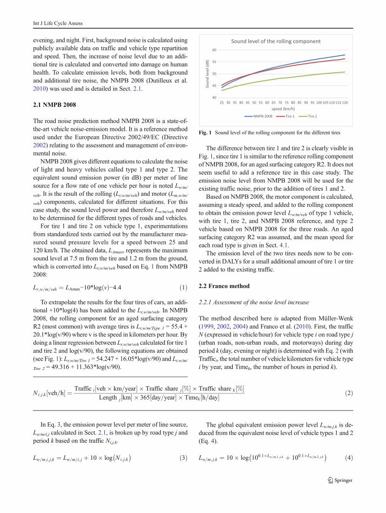
evening, and night. First, background noise is calculated usingpublicly available data on traffic and vehicle type repartitionand speed. Then, the increase of noise level due to an addi-tional tire is calculated and converted into damage on humanhealth. To calculate emission levels, both from backgroundand additional tire noise, the NMPB 2008 (Dutilleux et al.2010) was used and is detailed in Sect. 2.1.

2.1 NMPB 2008

The road noise prediction method NMPB 2008 is a state-of-the-art vehicle noise-emission model. It is a reference methodused under the European Directive 2002/49/EC (Directive2002) relating to the assessment and management of environ-mental noise.

NMPB 2008 gives different equations to calculate the noiseof light and heavy vehicles called type 1 and type 2. Theequivalent sound emission power (in dB) per meter of linesource for a flow rate of one vehicle per hour is noted Lw/m/

veh. It is the result of the rolling (Lr,w/m/veh) and motor (Lm,w/m/veh) components, calculated for different situations. For thiscase study, the sound level power and therefore Lw/m/veh needto be determined for the different types of roads and vehicles.

For tire 1 and tire 2 on vehicle type 1, experimentationsfrom standardized tests carried out by the manufacturer mea-sured sound pressure levels for a speed between 25 and120 km/h. The obtained data, LAmax, represents the maximumsound level at 7.5 m from the tire and 1.2 m from the ground,which is converted into Lr,w/m/veh based on Eq. 1 from NMPB2008:

Lr;w=m=veh ¼ LAmax−10*log vð Þ−4:4 ð1Þ

To extrapolate the results for the four tires of cars, an addi-tional +10*log(4) has been added to the Lr,w/m/veh. In NMPB2008, the rolling component for an aged surfacing categoryR2 (most common) with average tires is Lr,w/m/Type 1 = 55.4 +20.1*log(v/90) where v is the speed in kilometers per hour. Bydoing a linear regression between Lr,w/m/veh calculated for tire 1and tire 2 and log(v/90), the following equations are obtained(see Fig. 1): Lr,w/m/Tire 1 = 54.247 + 16.05*log(v/90) and Lr,w/m/Tire 2 = 49.316 + 11.363*log(v/90).

The difference between tire 1 and tire 2 is clearly visible inFig. 1, since tire 1 is similar to the reference rolling componentof NMPB 2008, for an aged surfacing category R2. It does notseem useful to add a reference tire in this case study. Theemission noise level from NMPB 2008 will be used for theexisting traffic noise, prior to the addition of tires 1 and 2.

Based on NMPB 2008, the motor component is calculated,assuming a steady speed, and added to the rolling componentto obtain the emission power level Lw/m/veh of type 1 vehicle,with tire 1, tire 2, and NMPB 2008 reference, and type 2vehicle based on NMPB 2008 for the three roads. An agedsurfacing category R2 was assumed, and the mean speed foreach road type is given in Sect. 4.1.

The emission level of the two tires needs now to be con-verted in DALYs for a small additional amount of tire 1 or tire2 added to the existing traffic.

2.2 Franco method

2.2.1 Assessment of the noise level increase

The method described here is adapted from Müller-Wenk(1999, 2002, 2004) and Franco et al. (2010). First, the trafficN (expressed in vehicle/hour) for vehicle type i on road type j(urban roads, non-urban roads, and motorways) during dayperiod k (day, evening or night) is determined with Eq. 2 (withTraffici, the total number of vehicle kilometers for vehicle typei by year, and Timek, the number of hours in period k).

N i; j;k veh=h½ � ¼Traffic i veh� km=year½ � � Traffic share j %½ � � Traffic share k %½ �

Length j km½ � � 365 day=year½ � � Timek h=day½ �ð2Þ

In Eq. 3, the emission power level per meter of line source,Lw/m/i,j calculated in Sect. 2.1, is broken up by road type j andperiod k based on the traffic Ni,j,k.

Lw=m;i; j;k ¼ Lw=m=i; j þ 10� log N i; j;k

� �

ð3Þ

The global equivalent emission power level Lw/m,j,k is de-duced from the equivalent noise level of vehicle types 1 and 2(Eq. 4).

Lw=m; j;k ¼ 10� log 100:1�Lw=m;1; j;k þ 100:1�Lw=m;2; j;k� �

ð4Þ

40

45

50

55

60

25 30 35 40 45 50 55 60 65 70 75 80 85 90 95 100 105 110 115 120

So

un

d le

vel

(dB

)

speed (km/h)

Sound level of the rolling component

NMPB 2008 Tire 1 Tire 2

Fig. 1 Sound level of the rolling component for the different tires

Int J Life Cycle Assess

The aim is now to evaluate the effect on this global soundemission power of additional vehicles equipped with the tiresstudied. An increase of 0.01 vehicle-kilometers from vehicletype 1 (adapted for tires 1 and 2) was considered, while trafficfor vehicles of type 2 stays identical. Only the rolling compo-nent Lr,w/m was added since the additional impact of the tirenoise is analyzed and not of the whole vehicle (excluding themotor component Lm,w/m). But even taking it into accountwould not have made a big difference because at the speedsused in this case study, the motor component is negligiblecompared to the rolling component. The rationale of settingsuch a marginal increase (0.01 vehicle-kilometers) is to assurelinearity between vehicle amount and sound power level. Theadditional sound power relative to the traffic increase is cal-culated in Eq. 5 and used to determine the equivalent soundemission power level L’w/m,j,k (as in Eq. 4).

L0w=m;TireX; j;k

¼ 10�log N 1; j;k � 100:1�Lw=m;1;i; j þ 0:01� 100:1�Lw=m;TireX;i; j� �

ð5Þ

The difference ΔLw/m,TireX,j,k between L’w/m,j,k and Lw/m,j,krepresents the marginal increase of noise level due to the ad-dition of 0.01 vehicle-kilometers of the rolling component oftype 1 vehicle equipped with four tires BTire X^ (X = {1,2})on each type of road j during each time period k. To obtain theimpact of 1 km driven, ΔLw/m,TireX,j,k is first divided by∆Vkmj,k, amount of vehicle-kilometers responsible for the ad-ditional 0.01 vehicle-kilometers of the rolling component oftype 1 vehicle for road j during period k (Eq. 6). The resultrepresents the increment in emission power level due to onevehicle-kilometer driven on road j during period k, which can

be distributed for the whole network and day period based ontraffic shares (δLw/m,TireX,j,k calculated with Eq. 7).

ΔVkm j;k veh� km=year½ � ¼ 0:01 veh=h½ �

� 365 day=year½ �

� Timek h=day½ �

� Length j km½ � ð6Þ

δLw=m;TireX; j;k

¼ΔLw=m;TireX; j;k � Traffic share j � Traffic sharek

ΔVkm j;kð7Þ

Franco et al. (2010) used Lden (day-evening-night equiva-lent level, based on Eq. 8) as the primary indicator for theevaluation of environmental noise.

Lden ¼ 10�log12

24�10

Lday10 þ

4

24� 10

Leveningþ5ð Þ10 þ

8

24� 10

Lnightþ10ð Þ10

!

ð8Þ

The factors represent period durations, with a poten-tial penalty (5 dB for evening and 10 dB for night) toreflect their importance to human perception. The dif-ference between sound emission power level Lw/m,k andLk (Eq. 8) for period k depends only on the geometryconsidered and is named A, for the sake of simplicity.

Calculating the Lden by road type j, Eq. 9 is obtained:

Lden; j ¼ 10� log12

24�10

Lwm; j;dayþA

10 þ4

24� 10

L wmj

;eveningþAþ5

� �

10 þ8

24� 10

Lwm; j;nightþAþ10ð Þ

10

0

B

@

1

C

A

¼ 10� log12

24�10

Lw=m; j;day10 þ

4

24� 10

Lw=mj;eveningþ5ð Þ10 þ

8

24� 10

Lw=m; j;nightþ10ð Þ10

!

þ A ð9Þ

L’den,j, the day-evening-night equivalent level obtained af-ter the addition of one vehicle-kilometer over the whole net-work and the whole day, is described in Eq. 10.

L0den;TireX; j ¼ 10� log12

24�10

Lw=m; j;dayþδLw=m;TireX; j;day10 þ

4

24� 10

Lw=mj;eveningþδLw=m;TireX; j;eveningþ5ð Þ10 þ

8

24� 10

Lw=m; j;nightþδLw=m;TireX; j;nightþ10ð Þ10

!

þ A ð10Þ

Subtracting Lden,j to L’den,TireX,j, the increment in day-evening-night equivalent level on road type j due to the

addition of one vehicle-kilometer over the whole networkand the whole day is obtained. Doing this, one can then

Int J Life Cycle Assess

observe that the term A has absolutely no importance since thesubtraction cancels it. The last step to obtain the increment inday-evening-night equivalent levels due to one vehicle-kilometer over the whole network and the whole day is asummation on j as shown in Eq. 11. Since the normalizationhas been done before, this is basically an averaging of ∆Lden,jover the different type of roads respecting the traffic sharebetween these roads.

δLden;TireX ¼ ∑j

L0den;TireX; j−Lden; j� �

ð11Þ

2.2.2 Assessment of the additional number of highly annoyed

people

The assessment of the additional number of highly annoyedpeople is one of the improvements of Franco et al. (2010)compared to Müller-Wenk (1999, 2002, 2004) and Doka(2003). It is based on the work of Miedema and Oudshoorn(2001) giving the polynomial approximations of the dose re-sponse curves relating Lden levels at the most exposed façadeof dwellings and self-reported annoyance. The exposure of thepopulation in Lden has been extracted from the strategic noisemap, calculated by different cities under the EuropeanDirective 2002/49/EC, and given in a number of peopleNp(g) exposed to noise level in decibel range g of 5 dB.

Franco et al. (2010) differentiated the polynomial approx-imation from Miedema and Oudshoorn (2001) for the centerof each decibel range. The result ∆%HA/∆Lden is the addition-al percentage of highly annoyed people by additional numberof decibels around this point. Doing this for each decibel rangeg, the additional number of highly annoyed people is deter-mined (Eq. 12).

ΔHATireX ¼ ∑g

N p gð Þ �Δ%HA=ΔLden gð Þ � δLden;TireX ð12Þ

Franco et al. (2010) considered the additional number ofhighly annoyed people to be a good midpoint for the integra-tion of noise in LCA. However, to compare this method withthe one developed in Cucurachi et al. (2012) and Cucurachiand Heijungs (2014), this result needs to be converted inDALYs.

2.2.3 Assessment of the DALYs per additional highly annoyed

people

The World Health Organization (Fritschi et al. 2011) made areview of the studies linking health impact and annoyance(highly annoyed people calculated from Lden level) and rec-ommended a disability weight (DW) factor of 0.02 DALY/highly annoyed people (uncertainty range 0.01–0.12), whichis therefore used in this study.

2.3 Cucurachi method

The methodology translates sound powers (in Joules) into thenumber of people that are exposed to a certain sound pressurefor a certain period of time (in person-Pa*s). The characteri-zation factors (in Person-Pa*W) related to elementary flows(in J) are calculated for archetypal situations depending ontheir frequency (eight octave bands), their time period (day,evening, and night), and their place (urban, suburban, rural,industrial, indoor). Cucurachi and Heijungs (2014) also pro-posed an Excel sheet to develop user-defined characterizationfactors, which could not be used due to the lack of availableinput parameters (e.g., temperature, relative humidity, distancefrom source to receiver, background noise). Regarding thearchetypal characterization factors, the measurements of thetire manufacturer are given in dB(A) (dB values aggregatedand weighted across frequency range) and only factors forunspecified frequency (calculated with central frequency of1000 Hz) could be applied.

The NMPB 2008 methodology determines the sound pow-er level of a source Lw from the emission power level permeter of line source for a flow rate of 1 vehicle per hourLw/m/veh using Eq. 13.

Lw;TireX ¼ Lr;w=m=TireX þ 10*log10 vð Þ þ 30 ð13Þ

Based on the speed and the Lw/m on the different roads, thesound power level of the rolling component (due to tires) canbe calculated for each road. The sound power level differen-tiated per type of road j in dB(A) can be converted into soundpower in Watts via Eq. 14 where Wref = 1 pW (ISO 9613-2,1996).

W TireX; j ¼ W ref � 10Lw;TireX; j=10 ð14Þ

To express sound power valuesWj for the functional unit inJoules, one vehicle-kilometer is split between the differentroad types and time thanks to the traffic share values, and thendivided by the mean speed. The obtained time Tj,k representsthe time one vehicle should spend on each road type j duringeach period k to create this additional one vehicle-kilometer inthe system. In other words, Eq. 15 represents the time ofemission of the corresponding source.

T j;k s½ � ¼1 km½ � � Traffic share k %½ � � Traffic share j %½ � � 3600

s

h

h i

speed j

km

h

� �

ð15Þ

The sound energy Ej,k (in Joules), product of Tj,k andWj, ismultiplied by the corresponding characterization factor de-fined by Cucurachi and Heijungs (2014), depending on geo-graphical (rural conditions considered for motorways andnon-urban paths) and temporal contexts (day period).

Int J Life Cycle Assess

The classification of the roads defined in this study doesnot fit the predefined situations from Cucurachi (e.g., Bnon-urban road^ includes suburban and rural locations); this willbe discussed later. The differentiated impacts obtained (in per-son-Pa*s) are summed up at the midpoint. In the last step, theimpacts obtained in person-Pa*s are converted to DALYswithone of the two mid_to_end conversion factors proposed byCucurachi and Heijungs (2014) based on de Hollander et al.(1999) and the WHO study (Fritschi et al. 2011). As stated bythe authors, these factors may be used to provide a measure ofthe noise impacts at the endpoint level. However, the authorsalso warned against uncertainties due to the assumption oflinearity. Comparing the results obtained from these factorswith the ones calculated with another method can be a goodway to assess the reliability of the factors.

3 LCA of tires without noise consideration

3.1 Goal and scope definition

Since the aim of the study is also to evaluate the contributionof noise to human health damage as compared to other envi-ronmental burdens, a comprehensive LCAwas carried out fortire 1 and tire 2. The LCA included the production of rawmaterials, car tire production, retailing, use of the tire, andseveral end-of-life pathways, for a functional unit defined asthe use of one tire over 1 km. The corresponding inventorydata is described in the next paragraphs.

3.2 Life cycle inventory

Inventory data for tire 1 was taken from PRé Consultants(2001) and further updated to reflect the current backgroundprocesses and use situations (e.g., share of end-of-life routes).For tire 2, representative data for the year 2010 was collectedfrom the tire manufacturer. In order to express the inventoryflows according to the functional unit, an average mileageduring the lifetime of the tire is considered, respectively40,000 and 46,000 km for tire 1 and tire 2.

3.2.1 Raw materials and tire production

The consumption and transport of raw materials were basedon the composition of the tires. Some simplifications werenecessary because of the lack of inventory data for a fewraw materials and for confidentiality reasons. Firstly, all thetypes of synthetic rubber were merged into only one category,as well as for accelerators, anti-degradant, textile, and wires.The type of resin was unspecified, and therefore, phenolicresin was considered as a proxy. Finally, no specific data couldbe gathered for the retarder, adhesion promoter, co-salt, andpeptizer, which were therefore excluded from the life cycle

inventory (LCI). These materials represent less than0.16 % of the tire mass, and therefore, their contributionto the overall environmental impact of the tire is likelyto be negligible. For the production of tires, energyconsumption (electricity and natural gas) and relatedemissions were estimated according to data from the tiremanufacturer, completed by information from ecoinvent2.2 (Frischknecht et al. 2005; PRé Consultants 2001).

3.2.2 Use phase

Two parameters were taken into account for the use phase: tiredebris emissions and fuel consumption. The total amount oftire debris was retrieved from PRé Consultants (2001) and isequal to 30 mg/km. The composition of tire debris was basedon measurements by the tire manufacturer and from literaturedata (ETRMA 2010; Ntziachristos and Boulter 2009; Null1999; PRé Consultants 2001; Rauterberg-Wulff 2003; TenBroeke et al. 2008), including particulate matter (with a diam-eter equal or lower than 10 and 2.5 μm), polycyclic aromatichydrocarbons, distillate aromatic extract (treated or not), andoil and zinc emissions.

To calculate the fuel consumption linked to the tire, theaverage car fuel consumption was estimated and allocated tothe tire. From PRé Consultants (2001), the average consump-tion for a car is 7.5 L/100 km with a share of 50/50 betweengasoline and diesel cars. Considering the mean sensitivityfriction coefficient, the authors estimated a consumption of1.2 L/100 km for the four tires. This data was taken intoaccount for tire 1 while the consumption of tire 2 was basedon the gain of rolling resistance (7.8 kg/kg instead of 10.5 kg/kg for the tire 1). Based on literature (ChemRisk 2009; Evanset al. 2009; Krzyżanowski et al. 2005; Weissman et al. 2003),0.26 % of fuel reduction is obtained per 1 % of rolling resis-tance reduction. The fuel consumption is therefore 0.7 L/100 km for four tires in the case of tire 2.

3.2.3 End-of-life of tires

The end-of-life route data was provided by the tire manufac-turer and taken into account retreading (8 %), direct reuse/export (10 %), material recovery (40 %), energy recoveryvia incineration in cement kilns and power plants (38 %),and landfill (4 %).

3.3 Life cycle impact assessment

The ReCiPe (Goedkoop et al. 2009) method, following thehierarchist perspective and average weighting set (H, A),was chosen for the assessment at endpoint level (impacts onhuman health, ecosystems, and resources expressed inDALYs, species, year and dollars, respectively). The integra-tion of noise impacts in DALYs is therefore possible and can

Int J Life Cycle Assess

be compared with other impacts on human health such asclimate change, ozone depletion, or human toxicity.

4 Evaluation of the reliability of the noise impact

assessment

4.1 Data inventory

This part concerns the collection of data (related uncertaintiesdetailed in Sect. 4.2). The lengths of each road type are issuedfrom the Trade Union of French Road Industry (USIRF©,n.d.), relative to 2009, and were found similar to the ones fromUNECE database and European statistics database (BEurostat,European Commission [WWWDocument], n.d.^). The aver-age speed on each type of road is taken from the French RoadSafety organization (French Road Safety reports, ObservatoireNational Interministériel de la Sécurité Routière (ONISR)[WWW Document] (n.d.)). These parameters are listed inTable 1.

The road traffic was obtained by averaging several sourcesand time series from the UNECE database (Lacour andJoumard 2002) and the French Road Safety organization(French Road Safety reports, Observatoire NationalInterministériel de la Sécurité Routière (ONISR) [WWWDocument] (n.d.): 430 billions of vehicle-kilometers for cars(type 1) and 29 billions of vehicle-kilometers for trucks.

Finding relevant data for the traffic distribution among thetime periods is not trivial. The data listed in Table 2 is issuedfrom a vast area around Lyon (France) and were provided byAcoucité (BObservatoire de l’environnement sonore de laMétropole de Lyon [WWW Document], n.d.^) who realizedthe noise maps for the Lyon area.

The corresponding area represents 2.1 and 2.4 % of thetotal French traffic for vehicle types 1 and 2, respectively,and covers different situations (from urban to rural). It canbe therefore considered as a good representation for the wholecountry. Also, these values are similar to ones from Müller-Wenk (2002, 2004), i.e., 86.9 % during daytime and 13.1 %during nighttime.

French population equals to 64.5 million individuals at thebeginning of 2016 according to the French National Institute

of Statistics and Economic Studies (Institut national de lastatistique et des études économiques, INSEE [WWWDocument], n.d.). To apply the Franco method, the noise ex-posure of the population is also needed. No specific data isavailable covering the whole French population. However, theEuropeanDirective 2002/49/EC requires cities withmore than100,000 inhabitants to elaborate noise maps and calculate theexposure to noise of their population. The data has been col-lected for 2007 and 2012 (Noise Observation and InformationService for Europe, NOISE [WWWDocument], n.d., NOISEplatform, available at http://noise.eionet.europa.eu/). In thecase of France, the dataset for 2007 is more complete andtherefore used in this case study (Table 3).

The population exposed to more than 75 dB is excludedfrom the case study since the polynomial approximations fromMiedema and Oudshoorn (2001) are not verified after 75 dB.However, this limitation concerns only a very small percent-age of the population. The population under 55 dB is consid-ered as non-affected. It would have been better to know thepercentage of population in the 50–55-dB range, but there isno data available for this range. The population covered bythis study is around 22 million, i.e., 34 % of the whole popu-lation considered. The availability of accurate data for onlyone third of the considered population is a significant short-coming of the study. Moreover, data are concerned mostlywith cities with a population of more than 100,000 inhabi-tants, and one can expect a different exposure for smaller citiesand rural area.

The number of additional people highly annoyed by oneadditional decibel has been calculated for each middledecibel-range of exposure (Table 4). These coefficients aredifferent from the one of Franco et al. (2010). Despite theauthors’ claim, the factors used do not come from the polyno-mial approximation of the synthesis annoyance curves extract-ed from Miedema and Oudshoorn (2001) for percentage ofhighly annoyed people but from the one for lowly annoyedpeople. As a result, different coefficients are obtained which

Table 1 Traffic data inventoried

Roadtype

Length(km)

Average speedtype 1 (km/h)

Average speedtype 2 (km/h)

Percentage oftraffic (%)

Motorway 11,243 115 90 23

Non-urbanroad

387,018 80 75 47

Urbanroad

630,000 50 50 30

Table 2 Traffic distribution among the different periods of the day

Time period Percentage of type 1traffic (%)

Percentage of type 2traffic (%)

Day 72 70

Evening 21 15

Night 7 15

Table 3 French population’s exposure coming from the NOISEplatform

dB range 55–59 60–64 65–69 70–74 >75

Percentage of the population 22.9 % 21.3 % 15.7 % 9.0 % 1.6 %

Int J Life Cycle Assess

increase with the decibel-range instead of being relativelyconstant in the case of the equation for lowly annoyed people.

The collection of data shows that assessing the noise im-pact on a whole country leads to significant approximations,due to lack of data but also to the modeling approach. Forexample, assuming an average speed for a whole road net-work or uniform traffic over a whole country is not represen-tative of the reality. Noise varies quickly in space and time andcan only be assessed accurately over a specific location and ona short time scale. Studying noise impact over a large territoryforces the practitioner to make unrealistic assumptions, andthe result can only give a very approximate picture of reality.In order to achieve more accurate results, a smaller scale needsto be focused upon. Section 4.2 focuses on data uncertainty,whereas the pertinence of the approximations due to the modelitself is not considered.

4.2 Uncertainty distributions of models’ parameters

Uncertainty distributions were defined for all the parametersof the models. For most of them, only a few values wereavailable and therefore normal distributions were assumed,using the mean and standard deviation of the values to setthe distributions.

The mean and standard deviation of the Total number

of vehicle-km of type 1 and the Total number of vehicle-kmof type 2 were derived from UNECE database (Lacourand Joumard 2002) and the French Road Safety organiza-tion (French Road Safety reports, Observatoire NationalInterministériel de la Sécurité Routière (ONISR) [WWWDocument] (n.d.). For the length of the three types ofroad, it is considered as a reliable value, assuming a stan-dard deviation of 5 %. For the different average speeds,the distributions have been estimated with yearly datafrom the French national road safety website (ONISR).For the repartition of the traffic between the differenttypes of roads, data from Lacour and Joumard (2002)were taken (similar data for motorways found in aFrench national road safety website). The resulting distri-bution of traffic between road types based on thesesources is very different from the one considered byMüller-Wenk (2004), mostly due to national differencesin both road network and usage. To model uncertaintieson percentage data, a Dirichlet distribution was used (toensure a sum of 1), with assumed standard deviation

around 10 %. For the percentage of traffic between thedifferent periods of the day, the data used is consideredrepresentative of the French territory, therefore assuminga standard deviation around 4 %.

For the emission power level of tire 1 and tire 2, two typesof uncertainty have been defined. The first uncertainty, calleddBNMPB, comes from NMPB 2008, which gives a 95 % con-fidence interval of ±2.5 dB(A) for the rolling component, witha distribution similar to the Gaussian form. Therefore, a nor-mal distribution with a standard deviation of ±1.25 dB(A) waschosen for all the type 1 vehicles. NMPB 2008 gives a 95 %confidence interval of ±3.2 dB(A) for the rolling componentof type 2 vehicles. Calculating independently the uncertaintyof type 2 vehicles would not be correct, so the uncertainty fortype 2 is equal to dBNMPB/2.5*3.2.

The second source of uncertainty for the emission powerlevel of tire 1 and tire 2, called dBexp, comes from the mea-surements. dBexp has been defined as the minimum level ofdecibel required to envelop every measurement points withinLr,w/m/Tire x ± dBexp,Tire x. This error is dependent on the tire:±1.3 dB for tire 1 and ±1.8 dB for tire 2. These values havebeen set as the standard deviation of a normal distributioncentered on 0.

A standard deviation of 2 % was set for the populationnumber to represent the good quality of data from INSEE.

For the exposure of the population to Lden, extrapolation ofdata covering only a third of the total population can lead toimportant mistakes. To avoid additional hypothesis, the max-imum value for each decibel-range is the one from the NOISEplatform (big cities most exposed to environmental noise) andis multiplied by the percentage of concerned population toobtain the minimum value (i.e., no exposition for the popula-tion not covered by the NOISE platform). A uniform uncer-tainty distribution was set between this minimum and maxi-mum for the exposure in each decibel-range.

Concerning the number of additional people highlyannoyed by the additional decibels of Lden, uncertainties comefrom the exact position in a given decibel range because thiscoefficient is lower in the lower part of a given decibel rangethan in the upper part. A uniform distribution is defined basedon coefficients in both extremities.

The weighting factor linking additional highly annoyedpeople to DALYs have been modeled from Fritschi et al.(2011) values. To fit the median given by the WHO, twotriangular distributions have been used, one between the min-imum and the median and the other between the median andthe maximum. Then, when using these distributions, for asample of size N, N/2 elements are coming from eachdistribution.

Regarding the characterization factors for theCucurachi model, the author suggested an uncertainty oftwo orders of magnitude above and below the valuesspecified in Cucurachi and Heijungs (2014). A triangular

Table 4 Additional percentage of highly annoyed people by Lden at agiven exposure

dB 55 57.5 60 62.5 65 67.5 70

Δ%HA/ΔLden 0.64 0.78 0.95 1.17 1.42 1.71 2.03

Int J Life Cycle Assess

distribution has been chosen with a logarithmic base of10, where the median equals the characterization factorsby Cucurachi. As only two values for the Mid_to_end

factor are available, a uniform distribution has been setbetween these two values (as conservative hypothesis).

The different parameters, their mean, standard deviation,and distribution are given in Tables 5 and 6.

4.3 Sensitivity and uncertainty analysis methods

Sensitivity analysis is a recommended step by the ISO standards14040-14044 (ISO 2006) to observe the influence of the assump-tions and choices made during the LCI and LCIA phases. Withthe set of uncertainties described above, uncertainty and sensitiv-ity analyses have been made using the R software.

Table 5 Parameters and their uncertainty distribution for the Franco model

Franco model: parameters and their uncertainties

Parameter Mean(Baseline)

Standarddeviation

Distribution used

Total number of vehicle-km of type 1 4.30E+11 3.25E+10 Normal (429580500000., 32537748003.2381)

Total number of vehicle-km of type 2 2.90E+10 7.11E+9 Normal (28990750000., 7109647384.26396)

Motorways’ length 11,243 562 Normal (11243., 562.)

Non-urban roads’ length 387,018 19,351 Normal (387018., 19351.)

Urban roads’ length 630,000 31,500 Normal (630000., 31500.)

Motorways’ average speed of type 1 115 15 Normal (115., 15.)

Non-urban roads’ average speed of type 1 80 10 Normal (80., 10.)

Urban roads’ average speed of type 1 50 5 Normal (50., 5.)

Motorways’ average speed of type 2 90 8 Normal (90., 8.)

Non-urban roads’ average speed of type 2 75 5 Normal (75., 5.)

Urban roads’ average speed of type 2 50 5 Normal (50., 5.)

Percentage of traffic on motorways 23.0 % 9.2 % Dirichlet (4.6, 9.4, 6.0)

Percentage of traffic on non-urban roads 47.0 % 10.9 % Dirichlet (4.6, 9.4, 6.0)

Percentage of traffic on urban roads 30.0 % 10.0 % Dirichlet (4.6, 9.4, 6.0)

Percentage of traffic during the day of type 1 72.0 % 4.5 % Dirichlet (72, 21, 7)

Percentage of traffic during the evening of type 1 21.0 % 4.1 % Dirichlet (72, 21, 7)

Percentage of traffic during the night of type 1 7.0 % 2.5 % Dirichlet (72, 21, 7)

Percentage of traffic during the day of type 2 70.0 % 4.6 % Dirichlet (70, 15, 15)

Percentage of traffic during the evening of type 2 15.0 % 3.6 % Dirichlet(70, 15, 15)

Percentage of traffic during the night of type 2 15.0 % 3.6 % Dirichlet (70, 15, 15)

dBNMPB 0 1.25 Normal (0, 1.25)

dBexp,Tire 1 0 1.30 Normal (0, 1.3)

dBexp,Tire 2 0 1.80 Normal (0, 1.8)

Population 6.45E+7 1.29E+6 Normal (64500000, 1290000)

Percentage of exposed population 55–60 dB 22.90 % Uniform (0.229/3, 0.229)

Percentage of exposed population 60–65 dB 21.30 % Uniform (0.213/3, 0.213)

Percentage of exposed population 65–70 dB 15.70 % Uniform (0.157/3, 0.157)

Percentage of exposed population 70–75 dB 9.00 % Uniform(0.090/3, 0.090)

Additional percentage of highly annoyed per additional Lden55–60 dB

0.81 % Uniform (0.00639, 0.00954)

Additional percentage of highly annoyed per additional Lden60–65 dB

1.21 % Uniform (0.00954, 0.01418)

Additional percentage of highly annoyed per additional Lden65–70 dB

1.77 % Uniform (0.01418, .02029)

Additional percentage of highly annoyed per additional Lden70–75 dB

2.47 % Uniform (0.02029, .02789)

Weighting factor converting highly annoyed in DALYs 0.02 1/2 Triangular (0.01, 0.02, 0.02) 1/2 Triangular (0.02,0.02, 0.12)

In bold: target parameter in the multivariate distribution

Int J Life Cycle Assess

For the uncertainty analyses, a Monte Carlo approachwith two samples of 100,000 iterations was adopted.Regarding global sensitivity analysis, Sobol indices ofeach parameter were calculated using the soboljansen

function from the R package sensitivity, the samplesgenerated with Monte Carlo approach, 500 bootstrapreplicates, and a level for bootstrap confidence intervalsof 0.95. The first-order Sobol index Si represents thecontribution to the output variance of the main effectof parameter i, standardized by the total variance toprovide a fractional contribution. The total-effect Sobolindex STi measures the contribution to the output vari-ance, including all variance caused by its interactions,of any order, with any other input variables. The differ-ence between these two indices provides information onthe level of interaction in the system.

5 Results interpretation

5.1 Integration with other impact categories

When integrating noise impacts into the overall life cy-cle impacts of the tire, its contribution is 8.1 % for tire1 and 76.7 % for tire 2 with the Franco model. Thiscan be a surprising result because tire 1 produces morenoise than tire 2. However, other sources of DALYshave been considerably reduced between the two tires,in a bigger proportion than noise. This is because, de-spite the decrease in absolute value, the importance ofnoise between the different sources of DALYs has in-creased in tire 2 compared with tire 1. In the case ofthe Cucurachi model, the impact of noise is so high thatit accounts for almost 100 % for both tires.

Table 6 Parameters and theiruncertainties’ distribution for theCucurachi model

Cucurachi model: parameters and their uncertainties

Parameter Mean(baseline)

Standarddeviation

Distribution used

Motorways’ average speed of type 1 115 15 Normal (115., 15.)Non-urban roads’ average speed of

type 180 10 Normal (80., 10.)

Urban roads’ average speed of type 1 50 5 Normal (50., 5.)Percentage of traffic on motorways 23.0 % 9.2 % Dirichlet (4.6, 9.4, 6.0)Percentage of traffic on non-urban

roads47.0 % 10.9 % Dirichlet (4.6, 9.4, 6.0)

Percentage of traffic on urban roads 30.0 % 10.0 % Dirichlet (4.6, 9.4, 6.0)Percentage of traffic during the day of

type 172.0 % 4.5 % Dirichlet (72, 21, 7)

Percentage of traffic during theevening of type 1

21.0 % 4.1 % Dirichlet (72, 21, 7)

Percentage of traffic during the nightof type 1

7.0 % 2.5 % Dirichlet (72, 21, 7)

dB (NMPB) 0 1.25 Normal (0, 1.25)dB (exp ; tire 1) 0 1.30 Normal (0, 1.3)dB (exp ; tire 2) 0 1.80 Normal (0, 1.8)Characterization factor, motorways,

day32,500 Triangular (325, 32500, 3250000,

logbase = 10)Characterization factor, non-urban

roads, day32,500 Triangular (325, 32500, 3250000,

logbase = 10)Characterization factor, urban roads,

day448,000 Triangular (4480, 448000, 44800000,

logbase = 10)Characterization factor, motorways,

evening120,000 Triangular (1200, 120000, 12000000,

logbase = 10)Characterization factor, non-urban

roads, evening120,000 Triangular (1200, 120000, 12000000,

logbase = 10)Characterization factor, urban roads,

evening842,000 Triangular (8420, 842000, 84200000,

logbase = 10)Characterization factor, motorways,

night182,000 Triangular (1820, 182000, 18200000,

logbase = 10)Characterization factor, non-urban

roads, night182,000 Triangular (1820, 182000, 18200000,

logbase = 10)Characterization factor, urban roads,

night1,430,000 Triangular (14300, 1430000, 143000000,

logbase = 10)Mid to end factor 0.000213 Uniform (0.000029061, 0.000213)

In bold: target parameter in the multivariate distribution

Int J Life Cycle Assess

In most of the LCA studies, the impact of noise is not takeninto account. The results obtained in our case study show thatthe impact of noise can be the most important among thedifferent impacts on human health caused by a tire. This resultinvokes that more effort is needed toward the systematic inte-gration of noise into LCA. It however also raises many ques-tions. Are the noise assessment models representativeenough? Are they robust? Can they be improved? In theSect. 5.2, we will analyze in more detail the two studies andtry to shed light on weaknesses of the existing model.

5.2 Relative change

The first aspect when analyzing a noise impact assessmentmethod is how it reacts to noise differences in the inputs. Tocalculate the impact between the two tires on human health,the relative change calculated as in Eq. 16 must be analyzed.

Relative change ¼DALYTire 1−DALYTire 2

max DALYTire 1;DALYTire 2ð Þð16Þ

Using the baseline values, the Franco method gives arelative change of 64.8 % between the two tires. TheMonte Carlo sampling with 200,000 iterations gives, forthe relative change, a mean of 60.0 %, a median of64.7 %, and a standard deviation of 21.3 %. The relativechange in the Franco method seems reliable. This methodvalidates the improvement between tire 1 and tire 2, eventaking into account the important uncertainties, if they havebeen modeled appropriately.

The sensitivity analysis on the Franco method shows thattwo parameters, dBexp,Tire1 and dBexp,Tire2, account for 84 % ofthe sum of the first-order Sobol indices and 99.6 % of the sumof total-order Sobol indices. It means that the uncertainties ofthe noise emission levels of the two tires are responsible for avery large part of the uncertainty about the relative change inDALYs between tire 1 and tire 2. More precise measurementsof the noise emission levels of the different tires coupled withwell-defined and narrower uncertainty and better fitting ofmeasurement curves will lead to smaller uncertainty on therelative change. The difference between the Sobol indices ofdBexp,Tire1 (S = 0.33, ST = 0.36) and dBexp,Tire2 (S = 0.63,ST = 0.67) is probably due to the difference in the standarddeviation of these two parameters. The difference between thefirst-order and total-order Sobol indices indicates that there areonly a few interactions in this model.

Regarding the Cucurachi method, the baseline valuegives a relative change of 56.0 % between the two tires,while the uncertainty analysis leads to a mean of 55.4 %,a median of 63.0 %, and a standard deviation of 32.2 %.This method also validates the improvement between tire

1 and tire 2, even if it is slightly lower than that with theFranco method.

Based on the total-order Sobol indices for the Cucurachimethod, dBexp for tire 1 and tire 2, explaining 46.9 % of theoutput variance, and the characterization factors, 50.9 % ofoutput variance, are responsible for most of the result uncer-tainty. As for the Francomethod, the contribution of dBexp,Tire1is approximately half of the contribution of dBexp,Tire2.Looking into detail into the characterization factors, the onesfor urban roads have a higher contribution, probably becauseof the larger part of the population impacted. Concerning thetemporal period, day characterization factors are higher thanthose during evening and night, probably because most of thetraffic occurred during the day. Characterization factors have alarge contribution on the uncertainty of the relative changebecause they have wide uncertainty distribution, roughly de-termined from suggestion from Cucurachi. Developers ofcharacterization factors should provide detailed uncertaintydistributions in order to allow proper uncertainties and sensi-tivity analyses.

The two methods do not show big differences whenassessing the relative change between tire 1 and tire 2. In bothcases, tire 2 is better and the reduction in DALYs issignificant.

5.3 DALY score

To analyze the score in DALYs resulting from the twomethods, it has been chosen to focus on tire 1 as analyzingtire 2 would naturally give similar results.

The obtained values were compared to the ones of Müller-Wenk (2002) and Franco et al. (2010) to check their validity.The level increase for 1000 vehicle-kilometers was 5.00e-7dBA (measured as LAeq) for Müller-Wenk (2002) and 3.80e-7 dBA in Lden for Franco et al. (2010), compared to 1.64e-8dBAwith the base values of this study. This lower value canbe explained by the longer road network (1,028,261 km in-stead of 13,872 km in Franco et al. 2010). On the other hand,the traffic on non-urban and urban roads is lower, so theresulting background noise is lower, which explains the small-er difference in Lden than in road length. Concerning the an-noyance, Müller-Wenk (2002) found 3.8e-2 cases of commu-nication disturbance and Franco et al. (2010) found 1.3e-3additional cases of annoyance. This study identified 1.0e-2additional cases of annoyance for tire 1. Differences can beexplained by the lower Lden increase, counterbalanced by apopulation 20 times bigger. Despite the differences betweenthe models used, the results obtained here are in the sameorder of magnitude than the ones from these two studies. Itdoes not seem to have major errors in the adaptation andapplication of the chosen methodology.

In the case of the Franco method, a value of 5.00e-8DALYs has been found for 1 vehicle-kilometer for tire 1 using

Int J Life Cycle Assess

the base values. A Monte Carlo run with 200,000 iterationsgives a median of 3.90e-8 DALYs, a mean of 5.82e-8 DALYs,and a standard deviation of 4.89e-8 DALYs. Uncertainties donot radically change the mean value but show an importantstandard deviation. Based on the sensitivity analysis onMonteCarlo samples, two parameters, dBexp,Tire1 and disability

weight, account for 84.0 % of the sum of the first-orderSobol indices and 99.6 % of the sum of the total-order Sobolindices. The first one, dBexp,Tire1, was already discussed be-fore. The second one, disability weight, is based on theFritschi et al. (2011) with S = 0.71 and ST = 0.81. In the caseof the Franco method, to achieve a better accuracy of theresult, it seems that the focus has to be put on diminishinguncertainties to link annoyance and human health. This resultis coherent with the Fritschi et al. (2011) presenting this link asvery uncertain due to the intrinsic difficulty of assessing noiseimpact and shows the importance of refining it to improveassessment reliability.

In the case of the Cucurachi method, a value of 5.85DALYs (based on the mid_to_end factor calculated byCucurachi from the WHO study) has been found for 1vehicle-kilometer for tire 1 using the base values. A MonteCarlo run with 200,000 iterations gives a median of 9.74DALYs, a mean of 16.95 DALYs, and a standard deviationof 22.77 DALYs. The difference between the median and themean is probably coming from the form of uncertainties cho-sen for the characterization factors.

The Cucurachi method has never been applied, to ourbest knowledge, to any case study. This means that thereis no other point of reference to check the result validity.However, we will compare the values coming from thetwo different methods summarized in Table 7. Takingthe mean, the Franco method gives 5.82e-8 DALYs andthe Cucurachi method gives 16.95 DALYs. There aremore than eight orders of magnitudes between the twomethods! This is a huge difference even for LCA. Evenif noise impact can be seen as difficult to assess and mea-sure, it is improbable that the damage on human healthdue to 1 vehicle-kilometer driven by one tire is anythingnear unity. Between these two results, the one fromFranco seems more realistic and reliable. Moreover, theconsideration of uncertainties in the case of the Cucurachimethod leads to a range of possible results whose averageis increased by a factor 3 compared to the case of basevalues. This means that the uncertainties are not

responsible for the very significant difference observedon the results obtained from the two methods.

For the Cucurachi method, the sensitivity analysesshow a significant difference between the sum of thefirst-order Sobol indices 0.72 and the sum of the total-order Sobol indices 1.42. It indicates strong interactionsin the model. Looking at the total-order Sobol indices,uncertainties on the input parameters dBexp,Tire1 explains9.3 % of the output variance and uncertainties about theemission dBNMPB explains an additional 8.6 %. Thehighest contribution comes from the characterization fac-tors accounting for 53.0 % of the output variance (higherfor urban roads and daytime). Impact on the uncertaintyof one characterization factor among others is directlylinked to the contribution of this road/period into thewhole DALY score. The contribution to the output varianceof themid_to_end factor is 17.7 % despite a very conservativeassumption of a uniform distribution between the two valuesgiven in Cucurachi and Heijungs (2014). Diminishing theuncertainties on the output implies refining the characteriza-tion factors and the link between the midpoint chosen byCucurachi, person-Pa*s, and the endpoint in DALYs.However, taking into account the really high result inDALYs, there are probably other problems to treat beforelooking at the uncertainty of the output.

6 Discussion

The impact of an additional amount of sound power is verydependent on the geographical situation because it depends onthe affected population (thus density), the existing sound lev-el, the topography, the absorption characteristics of the envi-ronment, etc. A lot of different parameters play a role in theimpact of an additional noise; consequently, it can be difficultto elaborate generic characterization factors. However, a re-gionalization of the life cycle impact assessment is not veryuseful if there is not a similar regionalization of the life cycleinventory. In the methods applied here, the inventory is doneat the national scale and it does not fit the predefined arche-types from Cucurachi and Heijungs (2014). The motorwaysand non-urban roads of our study can be used with the arche-types of unspecified location (chosen for this study), of rurallocation, or of suburban location. To evaluate the impact of

Table 7 DALY score and uncertainty for the two methods

Base Median Mean Standard deviation

Franco 5.00E−08 3.90E−08 5.82E−08 4.89E−08

Cucurachi 5.85 9.74 16.95 22.77

Table 8 Different location used for the characterization factors

Cucurachi Unspecified Rural Suburban

Tire 1 5.85 0.63 4.23

Tire 2 2.57 0.36 2.20

Relative change 0.56 0.42 0.48

Int J Life Cycle Assess

this choice, we calculated the DALY score and relative changewith three different possibilities for the location of motorwaysand non-urban roads. Table 8 shows the importance of thischoice.

Our incapacity to fit the inventory into the predefined ar-chetypes does not explain the high result coming from theCucurachi method. Looking at Cucurachi and Heijungs(2014), it is possible that these mid_to_end factors have beenoverestimated. To calculate it, the L95 value, noise level (dB)exceeding 95 % of time, was used coming from the fullBANOERAC report (EASA 2009). Even without lookingmore into details into the methodology, it is understandablethat a noise level exceeding 95 % of the time can be verydifferent from the equivalent noise level of the same area(equivalent noise level often chosen as a measure of the envi-ronmental noise). It means that Cucurachi and Heijungs(2014) may have underestimated the background noise andthus the calculation of the midpoint for the studied zone.Consequently, the mid_to_end factors can be largelyoverestimated.

Moreover, Cucurachi and Heijungs (2014) calculate themid_to_end factors in two studies accounting for the totalimpact on noise damage on human health. This approach doesnot take into account the possible non-linearity of the problemas already stated by the authors. In order to have a betterestimation of the mid_to_end factors, we advise to use anincremental approach. LCA considers, in most cases, smallvariations around a base scenario assumed to be representativeof the current conditions. An incremental approach wouldgive a mid_to_end factor closer to the modeled situation andthus would allow decreasing the uncertainty from non-linearity.

Regarding the general philosophy of these two differentmethodologies, they have both their pros and cons. TheFranco method used an incremental approach to assess theadditional impact of noise of a small increment in a specificsituation. This methodology has been developed by severalauthors and seems to give reliable results. However, it needsa specific modeling numerous data on the considered situa-tion. This can be time-consuming and would not allow sys-tematic integration of noise impact in LCA. Also, it wouldonly be possible for the foreground system.

On the other hand, the advantage of the Cucurachi methodto use archetypal situations and precalculated characterizationfactors can lead to a quick and systematic integration of noisedamage on human health in both foreground and backgroundof LCA studies. Of course, this exercise remains very difficult,considering that the characterization factors should show suf-ficiently low variability within an archetype and should beeasily understandable and applicable. However, theCucurachi method failed to give a plausible result and it isquite difficult to know why and how to improve thismethodology.

We think that there may exist a way to conciliate these twodifferent approaches: use the first approach to generate char-acterization factors in a given number of archetypal situations.This third way may be a good compromise, using the strengthof the two studied methods. The best way to study the feasi-bility of such characterization factors and to calculate themseems to use up-to-date data and tools. The EuropeanDirective 2002/49/EC forces European cities of more than100,000 inhabitants to generate noise maps and to collectthe needed data. This data could be used with up-to-date noisepropagation software to study the change in exposure due toincrement in existing traffic in a large panel of situations.Using such GIS software and data can allow the elaborationof spatialized and temporalized characterization factors. Thispossibility will be studied in future work.

7 Conclusions

This study aimed to compare the noise impact on humanhealth of two different tires, based on existing LCA method-ology. The noise characterization is still marginal in LCAstudies, and the present paper compares two very differentavailable methodologies, allowing the comparison of theirresults. Since noise impact category is still in development,it was important to understand the applicability and the out-comes given by the available methodologies. The large con-tribution of noise effects on overall human health results withFranco and Cucurachi methods highlights the necessity tointegrate noise impact on human health in LCA. More re-search and efforts should be encouraged, toward the study ofnoise impact, its integration in LCA, and its mitigation.

Franco and Cucurachi results showed an impact decreaseof 60.0 and 55.4 %, respectively, thanks to the technical char-acteristics of tire 2, as compared to tire 1. The outcomes areconsistent between the two methods because they are of thesame order of magnitude and they also show the improvementefforts made at the design phase to decrease the noise emis-sions. A good way to significantly reduce impact from noiseemissions seems to work on the design of the tires. The twomethods give a very different result in terms of DALY scoreswith more than eight orders of magnitudes between them. Theresult given by the Cucurachi method seems to beoverestimated with several DALYs by kilometers for one tire.

Both methods have advantages and drawbacks. However,it can be possible to choose a third method, in-between, com-bining the strength of the approach initiated by Müller-Wenkand the one imagined by Cucurachi. To do so, an incrementalapproach used on accurate localized and temporalized dataprocessed with noise propagation software could providecharacterization factors for a set of archetypes. This wayseems a good compromise between both approaches, and wewill work on it in the near future.

Int J Life Cycle Assess

Acknowledgments The authors gratefully acknowledge the GoodyearInnovation Center (GYIC) Luxembourg, in particular Dr. GeorgesThielen, for having co-funded the study and provided data for the twotires and Vanessa Peardon from LIST for English proofreading. Thisresearch has been funded by the Luxembourg National Research Fund(FNR) under the project DyPLCA (INTER/ANR/13/10/DyPLCA).

References

Althaus H-J, de Haan P, Scholz RW (2009) Traffic noise in LCA. Int JLife Cycle Assess 14:560–570

ChemRisk L (2009) Tyre generic exposure scenario; Service lifeguidance

Cucurachi S, Heijungs R (2014) Characterisation factors for life cycleimpact assessment of sound emissions. Sci Total Environ 468–469:280–291

Cucurachi S, Heijungs R, Ohlau K (2012) Towards a generalframework for including noise impacts in LCA. Int J LifeCycle Assess 17:471–487

De Hollander AE, Melse JM, Lebret E, Kramers PG (1999) An aggregatepublic health indicator to represent the impact of multiple environ-mental exposures. Epidemiol 10:606–617

Directive E (2002) Directive 2002/49/EC of the European parliament andthe Council of 25 June 2002 relating to the assessment and manage-ment of environmental noise. Off. J. Eur. Communities 189

Doka G (2003) Ergänzung der Gewichtungsmethode für ÖkobilanzenUmweltbelastungspunkte’ 97 zu Mobilitäts-UBP’ 97. DokaÖkobilanzen Zurich

Dutilleux G, Defrance J, Ecotière D, Gauvreau B, Bérengier M, BesnardF, Duc EL (2010) NMPB-routes-2008: the revision of the Frenchmethod for road traffic noise prediction. Acta Acust United Acust96:452–462

EASA (2009) Background noise level and noise level from en routeaircraft final report

ETRMA (2010) Replacement of highly aromatic oils in tyres – FAQ andDEFINITIONS [WWW Document]. URL http://www.etrma.org/uploads/Modules/Documentsmanager/20100712-etrma-qanda—replacement-of-ha-oils-in-tyres.pdf

Eurostat, European Commission [WWWDocument], n.d. URL http://ec.europa.eu/eurostat/ (accessed 2.26.16)

Evans L, MacIsaac Jr J, Harris J, Yates K, Dudek W, Holmes J, Popio J,Rice D, Salaani M (2009) NHTSA tire fuel efficiency consumerinformation program development: phase 2—effects of tire rollingresistance levels on traction, treadwear, and vehicle fuel economy.East Lib. OH Natl. Highw. Traffic Saf. Adm

Franco V, Garraín D, Vidal R (2010) Methodological proposals for im-proved assessments of the impact of traffic noise upon humanhealth. Int J Life Cycle Assess 15:869–882

French Road Safety reports, Observatoire National Interministériel de laSécurité Routière (ONISR) [WWW Document], n.d. URLhttp://www.securite-routiere.gouv.fr (accessed 2.26.16)

Frischknecht R, Jungbluth N, Althaus H-J, Doka G, Dones R, Heck T,Hellweg S, Hischier R, Nemecek T, Rebitzer G (2005) Theecoinvent database: overview and methodological framework. Int.J. Life Cycle Assess 10:3–9

Fritschi L, Brown L, Kim R, Schwela D, Kephalopolous S (2011)Conclusions [Burden of disease from environmental noise:Quantification of healthy years life lost in Europe]. World HealthOrganisation

GoedkoopM, Heijungs R, Huijbregts M, De Schryver A, Struijs J, van ZelmR (2009) ReCiPe 2008. Life Cycle Impact Assess. Method WhichComprises Harmon. Categ. Indic. Midpoint Endpoint Level 1

Heutschi K (2004) des forêts et du paysage Suisse. Office fédéral del’environnement, Eidgenössische Materialprüfungs-undForschungsanstalt. Akustik, Geinoz D, Liengme J-D, 2004.SonRoad: modèle de calcul du trafic routier. OFEFP

Hofstetter P, Müller-Wenk R (2005) Monetization of health damagesfrom road noise with implications for monetizing health impacts inlife cycle assessment. J Clean Prod 13:1235–1245

Huijbregts M, Hertwich EG, Reijnders L (2006) Including human healthdamages due to road traffic in life cycle assessment of dwellings. IntJ Life Cycle Assess 11:64–71

Institut national de la statistique et des études économiques (INSEE)[WWW Document], n.d. URL http://www.insee.fr/fr/ (accessed2.26.16)

ISO E (2006) 14044: 2006. Environ. Manag.-Life Cycle Assess.-Requir.Guidel. Eur. Comm. Stand

Krzyżanowski M, Kuna-Dibbert B, Schneider J (2005) Health effects oftransport-related air pollution. WHO Regional Office Europe

Lacour S, Joumard R (2002) Parc, usage et émissions des véhiculesroutiers en France de 1970 à 2020

Miedema HM, Oudshoorn CG (2001) Annoyance from transportationnoise: relationships with exposure metrics DNL andDENL and theirconfidence intervals. Environ Health Perspect 109:409

Müller-Wenk R (1999) Life-cycle impact assessment of road transportnoise. Institut für Wirtschaft und Ökologie, Universität St. Gallen(IWÖ-HSG)

Müller-Wenk R (2002) Attribution to road traffic of the impact of noiseon health environmental series no. 339: noise. Int J Life CycleAssess 7:376–376

Müller-Wenk R (2004) A method to include in lca road traffic noise andits health effects. Int J Life Cycle Assess 9:76–85

Nielsen P, Laursen J (2005) Integration of external noise nuisance fromroad and rail transportation in lifecycle assessment. Dan. Environ.Prot. Agency Cph

Noise Observation and Information Service for Europe (NOISE) [WWWDocument], n.d. URL http://noise.eionet.europa.eu/ (accessed2.26.16)

Ntziachristos L, Boulter P (2009) EMEP/EEA air pollutant emissionsinventory guidebook 2009: road vehicle tyre and brake wear; roadsurface wear. Copenhagen. Eur. Environ. Agency

Null V (1999) Safe process oils for tires with low environmental impact.Kgk Kautsch Gummi Kunstst 52:6

Observatoire de l’environnement sonore de la Métropole de Lyon[WWW Document], n.d.. acoucité. URL http://www.acoucite.org/(accessed 2.26.16)

PRé Consultants B (2001) Life cycle assessment of an average Europeancar tyre. Comm. Eur. Car Tyre Manuf. BLIC Third Party Rep. 23

Rauterberg-Wulff A (2003) Tire wear as source of PAH,Umweltbundesamt, Berlin CSTEE/2003/18/4

Steven H (2005) Ermittlung der Geräuschemission von Kfz imStraßenverkehr. TÜV Nord Würselen

Ten Broeke H, Hulskotte J, Van Der Gon H-D (2008) Emissionestimates for diffuse sources Netherlands EmissionInventory—road traffic tire wear. TNO Built Environmentand Geosciences. US department of energy (USDE) [WWWDocumen t ] . URL h t t p : / / www. em i s s i e r e g i s t r a t i e .nl/ERPUBLIEK/documenten/Water/Factsheets/English/Road%20traffic%20tyre%20wear.pdf (accessed 2.26.16)

USIRF ©., n.d. Union des Syndicats de l’Industrie Routière Française(USIRF)

Weissman S, Sackman J, Gillen D, Monismith C (2003) Extending thelifespan of tires: final report. Symplectic Eng. Corp. Inst. Transp.Stud. Univ. Calif. Berkeley 23

Int J Life Cycle Assess

120

11 Annex II

Paper II

Meyer, R., Lavandier, C., Gauvreau, B., Benetto, E., 2017. Influence of the search radius in a noise prediction

software on population exposure and human health impact assessments. Appl. Acoust. 127, 63–73.

DOI: https://doi.org/10.1016/j.apacoust.2017.05.028

Technical note

Influence of the search radius in a noise prediction software onpopulation exposure and human health impact assessments

Rodolphe Meyer a,b,⇑, Catherine Lavandier b, Benoit Gauvreau c, Enrico Benetto a

a Luxembourg Institute of Science and Technology (LIST), 5, avenue des Hauts-FourneauxL-4362, Esch-sur-Alzette, Luxembourgb ETIS, UMR 8051, Université Paris Seine, Université Cergy-Pontoise, ENSEA, CNRS, 2 rue Adolphe Chauvin, 95302 Cergy-Pontoise Cedex, Francec Ifsttar, Laboratoire d’Acoustique Environnementale (LAE), Center of Nantes, CS4, 44344 Bouguenais Cedex, France

a r t i c l e i n f o

Article history:

Received 25 August 2016

Received in revised form 24 May 2017

Accepted 25 May 2017

Keywords:

Search radius

Noise prediction software

Environmental noise

Human health

a b s t r a c t

Engineering software products allow for quantifying environmental noise and a population’s exposure to

road traffic noise which can then be linked to human health damage. This paper investigates the impact

of the search radius, a parameter used in emission and propagation models, on noise exposure results.

The search radius is the threshold distance from which noise sources are not considered anymore in

the exposure assessment. To understand the influence of this parameter on the evaluation of population’s

exposure, the search radius has been successively fixed to three different values (500 m, 1000 m and

2000 m) in four different geographical situations (village, industrial, suburban and inner city). The result

of this investigation highlights several points. First, despite a search radius often fixed to 1000 m by noise

prediction software users, going up to 2000 m shows significant increase in population’s exposure.

Second, the impact of a change in search radius is very dependent of the presence of preponderant noise

sources. Third, increasing the search radius can quickly lead to an impractical calculation time. A solution

to avoid underestimating the exposure without increasing too much the calculation time may be to only

account for preponderant noise sources beyond a given distance.

� 2017 Elsevier Ltd. All rights reserved.

1. Introduction

Noise is defined as an unwanted sound. The impact of environ-mental noise on human health has been abundantly discussed byscientific communities in the last decades. The World HealthOrganisation (WHO) has provided a comprehensive review of thesestudies [1]. The impacts taken into account are cardiovascular dis-ease, cognitive impairment in children, sleep disturbance, tinnitusand annoyance. The WHO quantified the burden of disease fromenvironmental noise on human health, finding a range of burdenof 1.0–1.6 million disability-adjusted life year (DALYs) for WesternEurope. More than 90% of this amount is coming from sleep distur-bance and annoyance. This important burden of disease pushed theWHO to consider environmental noise as public health problem.

There are several sources for environmental noise, such astransportation (road, railway and aircraft traffic), industrial activi-ties, construction work, energy resources (wind turbine), andleisure activities. Among them, transportation, especially road traf-fic, is predominant. For example, in France, it has been estimated

that the health costs due to environmental noise are largely causedby road traffic (89%) [2]. For this reason, this paper focuses only onroad traffic.

In order to assess the impact of noise on human health, it is nec-essary to evaluate the population’s exposure. The European direc-tive 2002/49/CE [3] requires the assessment and management ofthe environmental noise for major European cities. One of the fast-est and most efficient ways to evaluate exposure is to generatenoise maps with prediction software using simplified sound prop-agation models. There are various noise emission and propagationmodels that can be used, including the ones developed under theEuropean projects IMAGINE or HARMONOISE and the FrenchNMPB08 method [4–7]. NMPB08 has been preferred because it ismore recent and more accurate than previous noise emission andpropagation models, as described in Ecotiere et al. [8]. Engineeringsoftware products allow for quantifying exposure to environmen-tal noise coming from road traffic for a given population (as wellas noise coming from railway traffic and industrial activities). Theyalso allow to take into account different scenarios such as the pres-ence of sound barriers, absorbing grounds, changes in road surfacecharacteristics, speed limits, and changes in traffic.

Once the exposure of the population has been calculated, itcan be linked with impacts on human health by following the

http://dx.doi.org/10.1016/j.apacoust.2017.05.028

0003-682X/� 2017 Elsevier Ltd. All rights reserved.

⇑ Corresponding author at: Luxembourg Institute of Science and Technology

(LIST), 5, avenue des Hauts-FourneauxL-4362, Esch-sur-Alzette, Luxembourg.

E-mail address: rodolphe.meyer@list.lu (R. Meyer).

Applied Acoustics 127 (2017) 63–73

Contents lists available at ScienceDirect

Applied Acoustics

journal homepage: www.elsevier .com/locate /apacoust

recommendations of the WHO [1]. In this paper, only the two majorimpacts will be calculated, i.e. annoyance and sleep disturbance. Thelink between exposure and human health is the percentage of highlyannoyed (HA) persons, in the case of annoyance, and the percentageof highly sleep disturbed (HSD) persons, in the case of sleepdisturbance. Knowing the exposure, the number of persons highlyannoyed and/or highly sleep disturbed can be calculated using thedose response curves given, respectively, by Miedema andOudshoorn [9] and Miedema and Vos [10].

When implementing this approach, several parameters have tobe optimized, e.g. the search radius. The search radius defines a cir-cle around a receiver point, where the sound sources inside thiscircle will be considered in the calculation while the sound sourcesoutside this circle will be neglected. It can be seen as the allowed‘‘maximum propagation distance”. Studying the impact of thissearch radius on population exposure assessment is the mainobjective of this paper.

2. Material and methods

2.1. Population exposure assessment

In this study, a noise prediction software called CadnaA [11] isused. Among the calculation parameters of CadnaA, the so called‘‘Max. Search Radius” is the parameter of interest for this paper.This parameter is also called ‘‘maximum path length” in the NMPB2008 methodological guide [12]. For the sake of simplicity, thissearch radius will be referenced as dmax. When taking the pointof view of a building, all roads within the dmax will be consideredto evaluate the noise level at which this building is exposed. Thevalue chosen for dmax can have a large impact on the noise levelcalculated on each building’s facade.

Despite the sensitivity to dmax, there is no imposed or even rec-ommended value for this parameter in the European directive2002/49/EC [3]. In most cases, a typical value of 1000 m is used[13,14]. According to the NMPB 2008, the method used in thispaper for the configuration of CadnaA, the dmax is valid up to2000 m [12].

On the one hand, a higher value for the maximum propagationdistance implies that more sources will be considered in the calcu-lation of the noise level on the studied façades. If the noise propa-gation software works properly and the simulation is well done, aresult with a higher dmax should give a result more representativeof the reality. On the other hand, the number of considered sourceswill grow at the same rate as the square of dmax since the numberof considered sources is proportional to the surface taken intoaccount in the calculation (assuming a homogeneous distributionof sources). Moreover, the dmax parameter also modifies the num-ber of potential reflection and ray paths. Thus the calculation timecan quickly become unpractical.

Since a value of 1000 m is the typical value used by peopleworking on noise maps [13,14], a dmax value of 1000 m is chosenas a reference point. It may be interesting to compare two differentchanges in the value of the search radius to evaluate the benefits offixing dmax at 2000 m instead of the mostly used value of 1000 m.As a result, it has been chosen to compare a doubling of dmax from500 m to 1000 m and from 1000 m to 2000 m.

In order to study the impact of the search radius, GeographicInformation System (GIS) data was used. It is given by a localFrench agency, Acoucité [14], and contains all the necessary infor-mation for the exposure assessment (roads, traffic, buildings,inhabitants, topography, ground characteristics, etc.). The area ofthe study is the Grand Lyon region that corresponds to the Metro-polis of Lyon, a French territorial authority. The GIS data has beenmanipulated with a free and open-source software: OrbisGIS [15].

For the spatial scale of the study, a geographical mapping of theFrench territory called IRIS (Aggregated Units for Statistical Infor-mation - Ilots Regroupés pour l’Information Statistique) was chosen.

IRIS is the basic unit for the collection and transmission of sta-tistical data coming from the French National Institute of Statisticsand Economic Studies (INSEE) [16]. These geographical areas(16100 IRIS in France in total) are on a district scale and containbetween 1800 and 5000 inhabitants. More importantly, IRIS arebuilt in a way to ensure homogeneity among geographic anddemographic criteria [17], and that is the main reason why theyhave been chosen for this analysis. Moreover, while IRIS are largeenough to contain hundreds of buildings to be evaluated for eachsituation, they are small enough to allow for a lot of different cal-culations. This leads to a large amount of results which could bestatistically analysed.

For each studied IRIS, all of the inhabited buildings in the areacontained in the IRIS itself and an additional buffer of 1000 m havebeen evaluated for three values of search radius (dmax = {500 m;1000 m; 2000 m}). The buffer was chosen to have a higher numberof evaluated buildings to ensure a real ‘‘signal” and not just some‘‘noise”. The purpose of the buffer was to add more points in thestudied cases by considering a larger area.

For each evaluated building, the noise level, L, is the maximumnoise level found at four meters above ground and at two meters infront of all the façades of the studied building, following the stan-dard of European directive 2002/49/CE [3]. The noise predictionsoftware gives noise levels Lday, Levening, Lnight and Lden. Lday, Leveningand Lnight that correspond, respectively, to the noise level duringday (6–18 h), evening (18–22 h), and night (22–6 h), while Lden isa day-evening-night equivalent level.

The few existing typologies for IRIS seem to be based on socio-economic factors (e.g. [18]). To our knowledge, there is no existingtypology based on environmental noise at the IRIS scale. There aresome typologies based on noise for urban situations, but they areat the street scale [19,20]. Nevertheless, the aim of this paper isnot to establish a noise typology of IRIS, but to show the influenceof the search radius on different types of IRIS. The studied IRIS havebeen chosen to cover the different possibilities with a relativelylow sampling rate. Four IRIS have been selected which are consid-ered to be representative of the different types of configurationsencountered in the Grand Lyon area. This choice regarding the geo-graphical areas will be discussed in Section 4.1. For the sake of sim-plicity, a nickname is given for each of the four studiedgeographical area: Village, Industrial, Residential and City. It has tobe noted that, as the four IRIS do not represent prototypes of anytypology, the so-called Village is a geographical area which is notnecessarily representative of every village.

In Fig. 1 representing the Village, the space between the twooutlines is the 1000 m buffer. It means that the noise level in frontof all the inhabited buildings contained inside the exterior outlinewill be predicted. All the black squares are buildings while the darkcurving lines are roads. Finally, the grey lines are contour lines rep-resenting the topography. The noise prediction model will searchfor all the noise sources at less than dmax from the studied building.

The Village is centred on a small town in a hilly landscape.Within the buffer and the search radius, the considered area ismore heavily urbanised than the IRIS alone, but it is one of the lessdensely inhabited areas in the Grand Lyon region. There is a rail-way line, but the road traffic is the only noise source consideredin this work. There are no major roads in the area, so the environ-mental noise is expected to be low.

In the Industrial area, Fig. 2, most of the buildings in the IRIS areuninhabited. This is because it is an industrial area with big build-ings and open space. Once again, railways are present but nottaken into account. It means that most of the inhabited buildingsthat will be evaluated are not in the IRIS itself but in the buffer.

64 R. Meyer et al. / Applied Acoustics 127 (2017) 63–73

The landscape is relatively flat. Some roads present very dense traf-fic, so the environmental noise is expected to be high.

In Fig. 3, most of the buildings in the IRIS and its buffer are res-idential houses. This small town is surrounded by crops. There is a

road with heavy traffic crossing the IRIS; in this flat landscape, thesound will propagate without encountering any obstacles, so theenvironmental noise is expected to be high. The south of the eval-uated zone is mostly uninhabited buildings.

Fig. 1. Geographical area nicknamed ‘‘Village”. The interior bold outline is the IRIS, and the exterior bold outline delimits the 1000 m buffer. The black squares are buildings,

the black lines define the road network, and the grey ones represent the topography.

Fig. 2. Geographical area nicknamed ‘‘Industrial”. The interior bold outline is the IRIS, and the exterior bold outline delimits the 1000 m buffer. The black squares are

buildings, the black lines define the road network, and the grey ones represent the topography.

R. Meyer et al. / Applied Acoustics 127 (2017) 63–73 65

Fig. 3. Geographical area nicknamed ‘‘Residential”. The interior bold outline is the IRIS, the exterior bold outline delimits the 1000 m buffer. The black squares are buildings,

the black lines define the road network, and the grey ones represent the topography.

Fig. 4. Geographical area nicknamed ‘‘City”. The interior bold outline is the IRIS, the exterior bold outline delimits the 1000 m buffer. The black squares are buildings, the

black lines define the road network, and the grey ones represent the topography.

66 R. Meyer et al. / Applied Acoustics 127 (2017) 63–73

In Fig. 4, one can see a very densely urbanised area. This isdowntown Lyon, hence the high population density. This is a flatterrain with a lot of roads, but with the speed limit in city, onecan expect medium environmental noise for such an area.

The most important characteristics of the four studied IRIS aresummarised in Table 1.

2.2. Environmental noise impact on human health

Using the CadnaA prediction software (Section 2.1), the expo-sure of the population to environmental noise is obtained throughLday, Levening, Lnight and Lden index. The WHO [1] quantifies the bur-den of disease using the DALY indicator defined by the followingequation:

DALY ¼ YLLþ YLD ð1Þ

This indicator combines two different metrics, the years of lifelost due to premature death (YLL) and the years lived with disabil-ity (YLD). The YLL are expressed by:

YLL ¼ N � L ð2Þ

where N is the number of deaths due to the studied condition, and Lis the standard life expectancy at age of death (expectancy – age atdeath). In this paper, the two major contributors to the DALYs com-ing from environmental noise are annoyance and sleep disturbance.In these two cases, there will not be any premature death, soYLL = 0. YLD can be estimated with the following equation:

YLD ¼ I � DW � D ð3Þ

where I is the number of incident cases for the studied condition,the disability weight (DW) reflects the severity of the disability ona scale from zero (no adverse health effects) to one (equivalent todeath), and D is the average duration of the disability in years.

Accounting only for annoyance and sleep disturbance, thehuman health impact calculated in this paper with the followingequation:

HH ¼ NHA � DWHA þ NHSD � DWHSD ð4Þ

NHA is the number of highly annoyed persons and NHSD the numberof highly sleep disturbed persons. The disability weights for annoy-ance (DWHA) and sleep disturbance (DWHSD) can be found in thestudy of the WHO [1] and are reported in Table 2.

The only step missing between population exposure to environ-mental noise and human health impact is calculating the numberof HA and HSD persons. The relationship from Miedema and Oud-shoorn [9] can be applied to obtain the number of highly annoyedpersons knowing noise exposure in terms of Lden for each buildingand the number of inhabitants. It is given by:

%HA ¼ 9:868 � 10�4 � ðLden � 42Þ3 � 1:436 � 10�2 � ðLden � 42Þ2

þ 0:5118 � ðLden � 42Þ ð5Þ

The relationship from Miedema and Vos [10] can be used toobtain the number of highly sleep disturbed persons knowing theexposure in terms of Lnight for each building and the number ofinhabitants:

%HSD ¼ 0:01486 � L2night � 1:05 � Lnight þ 20:8 ð6Þ

Using these formulas, the human health impact of environmen-tal noise can be linked to population exposure and calculated foreach of the four cases exposed in Section 2.1.

3. Results

3.1. Qualitative approach for noise levels

The change in Lden values resulting from a doubling of dmax iscalculated. In order to visualize this change for each evaluatedbuilding, the increase in the evaluated noise level is plotted versusthe noise level evaluated for the smaller value of dmax. The resultsare given for each geographical studied area in Fig. 5.

Fig. 5(a) and (b) show important increases in noise level for aninitial noise level between 25 and 40 dB(A). In Fig. 5(c–f), the mostimportant increases in the noise level are occurring between 40and 60 dB(A). As expected, environmental noise is lower in thesmall village than in IRIS near major roads.

Fig. 5 also shows another anticipated trend: the maximum dif-ference between the noise levels obtained when doubling dmax

decreases with the initial noise level. In other words, lower noiselevels are more sensitive to a change in maximum propagation dis-tance than higher noise levels. A given amount of acoustical powerwill lead to a higher increase in noise level when starting from alower initial noise level. This is a direct consequence of the loga-rithmic scale on which the decibel is built. The increase in noiselevel can be very important for lower initial noise level, as seenin Fig. 5(c), (e) and (f), where increases can exceed 10 dB(A).

It can be also observed that the four selected geographical areasrepresent different behaviours. Fig. 5(a–f) show a higher increasein noise level between 500 m and 1000 m than between 1000 mand 2000 m. On the contrary, (g) and (h) show a significantincrease in the noise levels for some of the evaluated buildingswhen the maximum propagation distance passes from 1000 m to2000 m but none for a change from 500 m to 1000 m. This beha-viour will be discussed later in Section 3.4.

3.2. Quantitative approach for noise levels

With the first approach considered in Fig. 5, it is hardly possibleto see the percentage of buildings undergoing an increase in noiselevel, as thousands of points are plotted. Moreover, an increase canonly be considered as relevant if it occurs at a noise level that hasan impact on human health and if it exceeds a certain threshold. Inthis study, a threshold of 1 dB(A) has been chosen, considering thatan increase of less than 1 dB(A) is negligible as it cannot be

Table 1

Main characteristics of selected IRIS.

Nickname IRIS Description Number of evaluated

buildings

Studied population Density

(inh/km2)

Village 692330000 Small village in a valley. 2408 9832 800

Industrial 692730101 Industrial zone and suburban area, near a road with dense traffic. 2865 14737 820

Suburban 692710104 Crops and residential area crossed by a road with dense traffic. 3563 29223 920

City 693830501 Heavily urbanised, in downtown Lyon. 4043 93923 18 000

Table 2

Disability weight for annoyance and sleep disturbance from the WHO.

Health problem Disability weight (DW)

Annoyance 0.02

Sleep disturbance 0.07

R. Meyer et al. / Applied Acoustics 127 (2017) 63–73 67

detected by the human ear, thus it is not worth the computationaleffort and calculation time.

Identifying the minimum sound level to be considered is diffi-cult. Based on the WHO [1], the lower limit is 45 dB(A) for Lnight

and 55 dB(A) for the Lden. This last part involves knowing exposureabove 45 dB(A) for Lnight, above 50 dB(A) for Levening, and above55 dB(A) for Lday. In order to show the impact of a change in dmax

related to the noise level exposure in a quantitative way, the

Fig. 5. Noise level increase for a doubling of dmax for our four IRIS (a) village, going from dmax = 500 m to dmax = 1000 m, (b) village, going from dmax = 1000 m to

dmax = 2000 m, (c) industrial, going from dmax = 500 m to dmax = 1000 m, (d) industrial, going from dmax = 1000 m to dmax = 2000 m, (e) suburban, going from dmax = 500 m to

dmax = 1000 m, (f) suburban, going from dmax = 1000 m to dmax = 2000 m, (g) city, going from dmax = 500 m to dmax = 1000 m, (h) city, going from dmax = 1000 m to

dmax = 2000 m.

68 R. Meyer et al. / Applied Acoustics 127 (2017) 63–73

relative number of evaluated buildings above these thresholdsundergoing a change in exposure higher than 1 dB(A) has been cal-culated. The results are given in Table 3.

With this second approach, it is possible to detect two differentbehaviours. In Village and City areas, the increase in noise levelexposure due to changes of dmax is very low. In these two IRIS, lessthan 5% of the buildings exposed to noise levels above 45 dB(A)undergo an increase superior to 1 dB(A) and none for the oneexposed to noise levels above 55 dB(A). However, in Industrial

and Suburban areas, a significant part of the evaluated buildingundergoes an increase of more than 1 dB(A), especially between45 dB(A) and 55 dB(A). In these two IRIS, a doubling of dmax hasmore impact on Lnight than on Lday or Levening. The night periodmay be more sensitive to a change in search radius because the dif-ference between heavily trafficked roads and the environmentalnoise due to the rest of the road network may be more important.

3.3. Impact on human health

In order to quantify the impact of environmental noise, it can beinteresting to push the analysis one step further. Following the rec-ommendation of the WHO [1]: the number of HA persons and thenumber of HSD persons can be calculated in these four geograph-ical areas (see Eqs. (5) and (6)). Knowing the numbers of HA andHSD persons in each case allows the calculation of the DALYs

due to environmental noise as detailed in Section 2.2. These threeindicators have been calculated for each maximum propagationdistance (Table 4).

The human health impact in Table 4 is calculated using Eq. (4)and the disability weights given in Table 2. Studying the impor-tance of HA and HSD on the human health impact in DALYs, theshare of HSD in the DALYs can be calculated as explained in the fol-lowing equation:

Share of HSD in the DALYs ¼NHSD � DWHSD

NHA � DWHA þ NHSD � DWHSD

ð7Þ

The bigger contribution comes from HSD ranging between 58%(Industrial, dmax = 2000 m) and 67% (Suburban, dmax = 500 m).While averaging on the whole table (12 values), the mean shareof HSD in the DALYs is 61%. Even if there are more HA persons,the higher disability weight for HSD is compensating. The studiedpopulation changes considerably between the Village and the City,which partially explains why there is a difference in the DALYs’amount. Dividing the amount in DALYs at dmax = 2000 m by thepopulation gives values ranging from 0.0022 DALYs/person forthe Village to 0.0087 DALYs/person for the City. On average, some-one living in the studied City loses 3.2 days of ‘healthy” life per yearwhile one living in the Village loses 0.79 days of ‘‘healthy” life peryear. It is not surprising to find a higher human health impact in

Table 3

Percentage of evaluated buildings in the four IRIS undergoing an increase in noise level exposure higher than 1 dB.

Village L(dmax = 1000) dmax = 1000 � dmax = 500 L(dmax = 2000) dmax = 2000 � dmax = 1000

Day Evening Night Day Evening Night

�45 dB(A) 4.8% 3.7% 0.0% �45 dB(A) 0.2% 0.3% 0.0%

�50 dB(A) 0.2% 0.0% 0.0% �50 dB(A) 0.2% 0.0% 0.0%

�55 dB(A) 0.0% 0.0% 0.0% �55 dB(A) 0.0% 0.0% 0.0%

Industrial L(dmax = 1000) dmax = 1000 � dmax = 500 L(dmax = 2000) dmax = 2000 � dmax = 1000

Day Evening Night Day Evening Night

�45 dB(A) 23.0% 21.0% 33.5% �45 dB(A) 18.1% 19.4% 48.9%

�50 dB(A) 17.7% 13.8% 8.4% �50 dB(A) 15.6% 15.6% 16.9%

�55 dB(A) 2.1% 1.4% 0.6% �55 dB(A) 1.2% 0.7% 0.1%

Suburban L(dmax = 1000) dmax = 1000 � dmax = 500 L(dmax = 2000) dmax = 2000 � dmax = 1000

Day Evening Night Day Evening Night

�45 dB(A) 29.0% 29.6% 38.8% �45 dB(A) 30.1% 33.0% 58.5%

�50 dB(A) 24.4% 24.3% 22.5% �50 dB(A) 25.3% 26.6% 27.2%

�55 dB(A) 7.3% 6.2% 3.2% �55 dB(A) 2.4% 1.6% 1.0%

City L(dmax = 1000) dmax = 1000 � dmax = 500 L(dmax = 2000) dmax = 2000 � dmax = 1000

Day Evening Night Day Evening Night

�45 dB(A) 0.0% 0.0% 0.0% �45 dB(A) 2.0% 1.9% 0.1%

�50 dB(A) 0.0% 0.0% 0.0% �50 dB(A) 0.7% 0.3% 0.0%

�55 dB(A) 0.0% 0.0% 0.0% �55 dB(A) 0.0% 0.0% 0.0%

Table 4

Number of highly annoyed persons, highly sleep disturbed persons and DALYs for each geographical area studied and each maximum propagation distance.

Geographical area Village Industrial Suburban City

Population 9832 14737 29224 93924

Number of highly annoyed persons dmax = 500 m 411 727 1655 15601

dmax = 1000 m 414 858 2200 15615

dmax = 2000 m 416 1010 2679 15641

Number of highly sleep disturbed persons dmax = 500 m 183 365 975 7207

dmax = 1000 m 183 380 1081 7213

dmax = 2000 m 183 398 1150 7227

Human Health Impact (DALYs) dmax = 500 m 21 40 101 816

dmax = 1000 m 21 44 120 817

dmax = 2000 m 21 48 134 819

R. Meyer et al. / Applied Acoustics 127 (2017) 63–73 69

a louder situation. However, the amount of days of healthy life lostis important and explains the concerns related to environmentalnoise.

Regarding the WHO report [1] and taking only into accountannoyance and sleep disturbance, between 922,000 and1,490,000 DALYs have been found for a population of 285 million.The numbers from this WHO report lead to an impact per personranging from 0.0032 DALYs/person to 0.0052 DALYs/person. Thequietest area studied in this work (0.0022 DALYs/person) is underthe mean for Europe while the noisy city (0.0087 DALYs/person) isover that mean value. Given the limited sampling of this study, itmakes no sense to evaluate an average, but the results havenonetheless the same order of magnitude.

One way to understand the importance of the amount found inDALYs concerning environmental noise is to take a look at theimpact of air pollution. Van Zelm [21] considered the humanhealth effects of fine particulate (PM10) and ozone in Europe. Theyfound 0.003 DALYs/person for a European average. It means thatthe impact on human health coming from environmental noiseis, to the current knowledge of scientists, in the same order of mag-nitude as the impact of fine particulate and ozone.

The focus of this work is the assessment of the increase of thethree indicators (HA, HSD, DALY), while increasing the maximumpropagation distance. In order to better understand the importanceof this increase, the results are normalized and exposed in Table 5.For example, when looking at the increase in the number of HApersons when dmax goes from 500 m to 1000 m, the percentageof HA people at 1000 m explained by the change will be (HA(1000 m)-HA(500 m))/HA(1000 m).

Table 5 shows two main results. First, in the Industrial andSuburban areas, the variation of the three indicators when increas-ing the maximum propagation distance is important. Up to 10% ofthe impact in DALYs can be explained by the change in dmax fromdmax = 1000 m to dmax = 2000 m. Thus the impact of increasing themaximum propagation distance to 2000 m can be very importantwhen evaluating environmental noise impact on human health.One has to keep this information in mind while looking at a DALYscore. It seems sensitive to parameters that are not always dis-cussed or even stated when the results of population exposureassessment are given (e.g. in the case of the application of the Euro-pean directive 2002/49/CE [3]).

The other major result is the presence of two different beha-viours. Table 5 shows normalized increases between 4% and 24%for the three indicators in both Industrial and Suburban areas,whereas there is almost no increase for Village and City areas. Theseresults are in agreement with the observations made previously(see Fig. 5 and Table 3). Heavily trafficked roads can explain thelarge difference between these two behaviours, as developed inthe next section.

3.4. Heavily trafficked roads

Table 1 shows that the geographical areas most affected by theincrease in the maximum propagation distance are the two that

contain a heavily trafficked road. Indeed, the Industrial and Subur-

ban area contain, or are adjacent to, roads with a daily trafficgreater than 2000 passenger cars per hour at a speed of 90 km/h.Fig. 6 presents all the roads with an hourly traffic higher than2000 passenger cars. The interior, bold, black outline is the IRIS,while the exterior, bold, black outline delimits the 1000 m buffer.The red, orange and yellow areas are areas located at less than500 m, less than 1000 m, and less than 2000 m, respectively, froma heavily trafficked road.

These heavily trafficked roads are the most important noisesources compared to the other roads taken into account in theexposure calculation. That is why they have an important impacton the noise level evaluated at buildings’ facades. If the changein the maximum propagation distance adds a heavily traffickedroad that was not considered before (a building in an orange or yel-low zone on Fig. 6), the noise exposure at the building undergoesan important increase (see Fig. 5(c–f) and Table 3 concerningIndustrial and Suburban). Fig. 6(b) and (c) show this phenomenonvery well with a large number of buildings in the orange and yel-low areas. If all the studied buildings are located under 500 m (inthe red area) or over 2000 m (in the white area) of all heavily traf-ficked roads, changing the search radius would not lead any build-ings to consider a heavy traffic road that was not consideredbefore, so it would change almost nothing in the exposure results.

Concerning the City, Fig. 5(g) and (h) and Table 3 show a similarbut less significant effect. Fig. 6(d) shows that there are less build-ings in the orange zone than in the yellow zone. That explains whya cluster of points can be seen well above the baseline (at 0 dB(A)),when dmax goes from 1000 m to 2000 m but not when dmax goesfrom 500 m to 1000 m. However, when looking at Fig. 6(d), onecan be surprised that the large amount of buildings in the orangezone do not have a higher impact compared to Industrial andSuburban. This difference is explained here by the fact that heavilytrafficked roads in this area are limited to 50 km/h and the sur-rounding noise is higher. Moreover, the high density of buildingsin the city creates a ‘‘mask effect”, which blocks some of the noisethat could reach another building’s façades.

If an IRIS is in the neighbourhood of a heavily trafficked road,the most influential parameter when assessing the importance ofa change of the search radius is the distance between studiedbuildings and heavily trafficked roads. The results for Village inTable 3 show that in the absence of heavily trafficked roads(Fig. 6(a)), the impact of a change in the search radius seems tobe lower when dmax goes from 1000 m to 2000 m than when dmax

goes from 500 m to 1000 m.

3.5. Calculation time

The drawback of a higher dmax is its longer calculation time, aresult of taking more roads into account. The calculation timesfor the four IRIS considered and different values of dmax are givenin Table 6.

Table 6 shows that the calculation time for a dmax value of2000 m is much higher than dmax = 1000 m, roughly a day instead

Table 5

Percentage of HA persons, HSD persons, and DALYs explained by the change in the search radius.

IRIS Village Industrial Suburban City

Increase in HA persons From 500 to 1000 m 0.8% 15.3% 24.8% 0.1%

From 1000 to 2000 m 0.3% 15.0% 17.9% 0.2%

Increase in HSD persons From 500 to 1000 m 0.4% 4.1% 10.8% 0.1%

From 1000 to 2000 m 0.0% 4.8% 6.4% 0.2%

Increase in DALYs From 500 to 1000 m 0.6% 8.4% 15.3% 0.1%

From 1000 to 2000 m 0.1% 9.0% 10.8% 0.2%

70 R. Meyer et al. / Applied Acoustics 127 (2017) 63–73

of few. If one needs to perform a lot of calculations or to calculate apopulation’s exposure over a large geographical area, choosingdmax = 2000 m may be impractical.

The calculation time per building varies with different geo-graphical areas. On the one hand, the Village area is a complex

landscape with a complex topography which implies a longer cal-culation of the noise propagation. In the other hand, the Suburban

area is significantly lower because it is a relatively flat landscapeand not densely urbanised.

In theory, due to the 2D geometry of the problem, the calcula-tion time per building should grow with the square of dmax if theroad network is uniform, growing in the same pattern as the sur-

face considered (p � d2maxÞ. If one plots the calculation time per

buildings, one will see that it follows roughly what was theoreti-cally predictable.

4. Discussion

4.1. General consideration

This study was carried out in a limited number of areas. Even ifthey were selected to represent very different situations, theyprobably do not represent all the possibilities. The Village,Industrial, Suburban and City areas likely do not represent everyvillage, industrial area, suburban residential area, or city found inFrance or around the world. However, to study a limited amount

Fig. 6. Influence of heavily trafficked roads. IRIS and buffer (bold outlines). Areas located at less than 500 m, 1000 m and 2000 m from heavily trafficked roads (respectively

red, orange and yellow areas). (a) Village, (b) industrial, (c) suburban, (d) city. (For interpretation of the references to colour in this figure legend, the reader is referred to the

web version of this article.)

Table 6

Calculation time for different values of dmax per the four IRIS studied.

Geographical

area

dmax

(m)

Calculation time

(min)

Calculation time by

buildings (s)

Village 500 85 2.1

1000 508 12.7

2000 1479 36.9

Industrial 500 68 1.4

1000 302 6.3

2000 959 20.1

Suburban 500 50 0.8

1000 184 3.1

2000 826 13.9

City 500 63 0.9

1000 241 3.6

2000 1548 23.0

R. Meyer et al. / Applied Acoustics 127 (2017) 63–73 71

of geographical area is not a problem because it is sufficient in find-ing some specific behaviours. A more exhaustive approach wouldbe necessary to validate the observations.

This study shows that the higher noise levels are more resistanttowards a change in the search radius than lower noise levels.Looking at the impact on human health coming from environmen-tal noise for low levels, such as 45 dB(A) or even 50 dB(A), can betricky because of the sensitivity of these noise levels to simulationparameters. The uncertainties regarding lower noise levels will besubstantially higher than the ones of high noise levels because oftheir higher sensitivity. These important changes in noise levelswhen changing the search radius are also visible in the results inDALYs, i.e. on the human health impacts of environmental noiseas it is calculated today. A practitioner calculating the burden ofdisease attributable to environmental noise must keep this in mindand interpret the results accordingly.

In the presence of heavily trafficked roads in the area of study orin the surroundings, the chosen search radius will have a stronginfluence on the result. The presence of a noise source strongerthan the majority of the noise sources in the studied zone can sig-nificantly affect the exposure of the evaluated buildings, particu-larly when a change in the search radius integrates a heavilytrafficked road in the calculation. To account for this, the searchradius should be adjusted according to different situations. If thearea has a heavily trafficked road, the search radius should beincreased to the possible maximum while it can be decreased inareas where the emission sound power level of the noise sourcesis relatively homogeneous. Applying this kind of rule on the GrandLyon area would imply the use of a search radius of 2000 m innearly all the IRIS because there are only few cases where thereis absolutely no influence from heavily trafficked roads. However,using 2000 m instead of 1000 m will considerably increase thetime of calculation (see Section 3.5).

A more elegant solution for this particular problem could be toassociate a search radius to each road, depending on the emissionnoise level of this specific road in absolute terms or compared tothe other noise sources in the surroundings. Above a given dis-tance, an evaluated building will not consider all the noise sourcesbut only the strongest, i.e. the heavily trafficked roads. Thismethodology would have the advantage of being more economicin terms of calculation effort, but it would need a change in theapproach used in the environmental noise prediction software. Inthe selected software, CadnaA, the same search radius is used foreach source without consideration for the relative importance ofa noise source compared with its surroundings.

Beyond this paper, the goal of this research is to integrate theimpact of environmental noise on human health in the frameworkof life cycle assessment (LCA). The need for accuracy and represen-tativeness is not the same in LCA as it is in acoustics: only a simpleand robust method is needed. A non-systematic method could becriticized for the possible biases coming from the operator’schoices. Nothing in this study justifies choosing a search radiusof 1000 m. On the contrary, the results presented here push towarda search radius of 2000 m. There is no theoretical reason to use admax of 1000 m instead of 2000 m, but there is a practical reason.A lot of calculations cannot be feasible with a search radius of2000 m.

4.2. Proposition

Taking a search radius of 2000 m can lead to high calculationtime. Since the presence of heavily trafficked roads seems to bethe most important parameter, these roads can explain a large partof the difference in the noise levels of exposure when the maxi-mum propagation distance is increased. Therefore, a good compro-mise could be to take into account the road networks at less than1000 m from the studied buildings and then only the major roadsbetween 1000 m and 2000 m.

In order to identify the feasibility of such proposition, an IRIShas been chosen where most buildings are located at a distancebetween 1000 m and 2000 m from all major roads. This IRIS is dif-ferent from the other ones in this paper and has been chosen onlyto satisfy this condition. All the 641 buildings in this IRIS are eval-uated. The whole population contained in this geographical area is1765 persons. The buildings and landscape have been picked insidea buffer of 2000 m around this area. The road network has beenentirely selected up to 1000 m and, depending on the case, thewhole road network or only the major roads between 1000 mand 2000 m have been picked. Three simulations were run: (1) amaximum propagation distance of 1000 m, (2) a maximum propa-gation distance of 2000 m and the whole road network, and (3) amaximum propagation distance of 2000 m but only major roadsbetween 1000 and 2000 m. The resulting calculation time is givenin Table 7 along with the three indicators studied in the previoussection: number of HA persons, number of HSD persons, andDALYs.

As expected, the three indicators and the calculation timeincrease with dmax. Taking into account all the roads instead of onlyheavily trafficked ones lead also to higher results, both in humanhealth impacts and calculation time. The calculation time ofScenario 2 is 4.6 times higher than Scenario 1. Scenario 3 providesa compromise between the two, with a calculation times 2.7 timeshigher than Scenario 1, but also greater coverage of noise-relatedhuman health impacts. Applying Scenario 3 instead of 2 leads saves40% of the calculation time. Additionally, Scenario 3 explains 76%of the change between Scenarios 1 and 2 in the number of HA per-sons, 82% of the change in the number of HSD persons, and 77% ofthe change in DALYs. In other words, considering only major roadsbetween 1000 m and 2000 m adds only half of the supplementarycalculation time but explains more than three quarters of thedifference in terms of HA persons, HSD persons or DALYs.

This small experiment is only qualitative because of technicalreasons. The buildings in the middle of the IRIS take into accountthe whole road network up to 1000 m plus their distance to theborder of the IRIS in each case. So this experiment is only a roughapproach to test this hypothesis on the importance of heavily traf-ficked roads with the available tools. Taking only one building intoaccount leads to a too quick calculation time to allow comparisonbetween scenarios, so this calculation had to be carried out on alarger scale. However, even doing the experiment on the single IRISand in an approximate manner, it shows a good compromise toobtain a more precise noise level evaluation without increasingthe calculation time too drastically. This proposed methodologymay be a path worth exploring to refine the calculations of noiseprediction software.

Table 7

Calculation time in the three different scenarios.

Scenario dmax (m) Road considered between 1000 m and 2000 m from the IRIS Calculation time (s) HA persons HSD persons DALYs

1 1000 None 1231 53.5 32.5 3.34

2 2000 All 5624 78.7 34.7 4.00

3 2000 Only roads with more than 2000 passenger cars by hour 3358 72.7 34.3 3.85

72 R. Meyer et al. / Applied Acoustics 127 (2017) 63–73

5. Conclusion

Studying the impact coming from a change in search radiushighlights several interesting elements. A search radius is oftenfixed to 1000 m by noise prediction software users, but a signifi-cant increase in the noise level evaluated can occur in some situa-tions when setting the search radius at 2000 m.

The impact of this change in the maximum propagation dis-tance is very dependent on the presence of one or several prepon-derant noise sources, such as a heavily trafficked road in a calm/quiet area. However, setting the search radius at 2000 m can beproblematic for practical reasons. In particular, the additional costin terms of calculation time may not be sustainable. Choosing themaximum distance propagation on a case to case basis can alsolead to criticism over the choices made by the operator.

An accommodating way to solve this problem could be to havea search radius depending on the emission noise level of the noisesources in absolute or relative terms. Noise prediction softwaremay look in this direction to integrate heavily trafficked roads inthe evaluation of noise exposure, allowing a more accurate evalu-ation of human health impacts without increasing too much thecalculation time.

Acknowledgement

This research has been funded by the Luxembourg NationalResearch Fund (FNR) under the project DyPLCA (INTER/ANR/13/10/DyPLCA).

References

[1] Fritschi L, Brown L, Kim R, Schwela D, Kephalopolous S. Conclusions [Burden ofdisease from environmental noise: Quantification of healthy years life lost inEurope]. World Health Organisation; 2011.

[2] ADEME CNB_Cout_social_des_pollutions_sonores_Rapport_2016_05_04.pdf.<http://www.bruit.fr/images/stories/pdf/ADEME%20CNB_Cout_social_des_pollutions_sonores_Rapport_2016_05_04.pdf> [accessed: 04-Jul-2016].

[3] Directive E. Directive 2002/49/EC of the European parliament and the Councilof 25 June 2002 relating to the assessment and management of environmentalnoise. Off J Eur Commun 2002; 189(12).

[4] Dutilleux G et al. NMPB-Routes-2008: the revision of the french method forroad traffic noise prediction. Acta Acust. United Acust 2010;96(3):452–62.

[5] IMAGINE. Guidelines for the use of traffic models for noise mapping and noiseaction planning. vol. Deliverable 7 of the IMAGINE (Improved methods for theassessment of the generic impact of noise in the environment) Project, TNOTechnical Report, Delft, The Netherlands; 2007.

[6] IMAGINE. The noise emission model for European road traffic. vol. Deliverable11 of the IMAGINE (Improved methods for the assessment of the genericimpact of noise in the environment) Project, M+P—Consulting EngineersTechnical Report, Vught, The Netherlands; 2007.

[7] van Maercke D, Defrance J. Development of an analytical model for outdoorsound propagation within the harmonoise project. Acta Acust United Acust2007;93(2):201–12.

[8] Ecotiere D, Foy C, Dutilleux G. Comparison of engineering models of outdoorsound propagation: NMPB2008 and Harmonoise-Imagine. Acoustics 2012;2012.

[9] Miedema HM, Oudshoorn CG. Annoyance from transportation noise:relationships with exposure metrics DNL and DENL and their confidenceintervals. Environ Health Perspect Apr. 2001;109(4):409.

[10] Miedema HME, Vos H. Associations between self-reported sleep disturbanceand environmental noise based on reanalyses of pooled data from 24 studies.Behav Sleep Med 2007;5(1):1–20.

[11] Computer Aided Noise Abatement; DataKustik, Greifenberg, Germany. <http://www.datakustik.com/en/products/cadnaa> [accessed: 01-Apr-2016].

[12] SETRA Copyright (Collective). Road noise prediction: NMPB 2008 - Noisepropagation computation method including meteorological effects.Methodological guide; 2009.

[13] Bruitparif, le bruit en Ile-de-France. <http://www.bruitparif.fr/> [accessed: 04-Jul-2016].

[14] Observatoire de l’environnement sonore de la Métropole de Lyon. acoucité.<http://www.acoucite.org/> [accessed: 26-Feb-2016].

[15] OrbisGIS official website. <http://orbisgis.org/> [accessed: 04-Jul-2016].[16] Institut national de la statistique et des études économiques (INSEE). <http://

www.insee.fr/fr/> [accessed: 26-Feb-2016].[17] Définition - IRIS | Insee. <https://www.insee.fr/en/metadonnees/definition/

c1523> [accessed: 30-Mar-2017].[18] Asterop : Le géomarketing décisionnel. <http://www.asterop.fr/fr/

produits/donnees/typologies_IRIS.html> [accessed: 04-Jul-2016].[19] Wang B, Kang J. Effects of urban morphology on the traffic noise distribution

through noise mapping: a comparative study between UK and China. ApplAcoust 2011;72(8):556–68.

[20] Silva LT, Oliveira M, Silva JF. Urban form indicators as proxy on the noiseexposure of buildings. Appl Acoust 2014;76:366–76.

[21] van Zelm R et al. European characterization factors for human health damageof PM10 and ozone in life cycle impact assessment. Atmos Environ 2008;42(3):441–53.

R. Meyer et al. / Applied Acoustics 127 (2017) 63–73 73

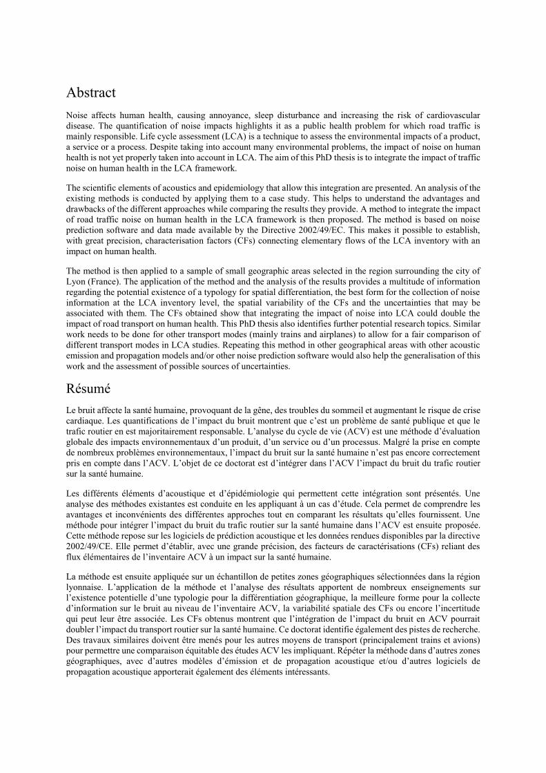
Abstract

Noise affects human health, causing annoyance, sleep disturbance and increasing the risk of cardiovascular disease. The quantification of noise impacts highlights it as a public health problem for which road traffic is mainly responsible. Life cycle assessment (LCA) is a technique to assess the environmental impacts of a product, a service or a process. Despite taking into account many environmental problems, the impact of noise on human health is not yet properly taken into account in LCA. The aim of this PhD thesis is to integrate the impact of traffic noise on human health in the LCA framework.

The scientific elements of acoustics and epidemiology that allow this integration are presented. An analysis of the existing methods is conducted by applying them to a case study. This helps to understand the advantages and drawbacks of the different approaches while comparing the results they provide. A method to integrate the impact of road traffic noise on human health in the LCA framework is then proposed. The method is based on noise prediction software and data made available by the Directive 2002/49/EC. This makes it possible to establish, with great precision, characterisation factors (CFs) connecting elementary flows of the LCA inventory with an impact on human health.

The method is then applied to a sample of small geographic areas selected in the region surrounding the city of Lyon (France). The application of the method and the analysis of the results provides a multitude of information regarding the potential existence of a typology for spatial differentiation, the best form for the collection of noise information at the LCA inventory level, the spatial variability of the CFs and the uncertainties that may be associated with them. The CFs obtained show that integrating the impact of noise into LCA could double the impact of road transport on human health. This PhD thesis also identifies further potential research topics. Similar work needs to be done for other transport modes (mainly trains and airplanes) to allow for a fair comparison of different transport modes in LCA studies. Repeating this method in other geographical areas with other acoustic emission and propagation models and/or other noise prediction software would also help the generalisation of this work and the assessment of possible sources of uncertainties.

Résumé

Le bruit affecte la santé humaine, provoquant de la gêne, des troubles du sommeil et augmentant le risque de crise cardiaque. Les quantifications de l’impact du bruit montrent que c’est un problème de santé publique et que le trafic routier en est majoritairement responsable. L’analyse du cycle de vie (ACV) est une méthode d’évaluation globale des impacts environnementaux d’un produit, d’un service ou d’un processus. Malgré la prise en compte de nombreux problèmes environnementaux, l’impact du bruit sur la santé humaine n’est pas encore correctement pris en compte dans l’ACV. L’objet de ce doctorat est d’intégrer dans l’ACV l’impact du bruit du trafic routier sur la santé humaine.

Les différents éléments d’acoustique et d’épidémiologie qui permettent cette intégration sont présentés. Une analyse des méthodes existantes est conduite en les appliquant à un cas d’étude. Cela permet de comprendre les avantages et inconvénients des différentes approches tout en comparant les résultats qu’elles fournissent. Une méthode pour intégrer l’impact du bruit du trafic routier sur la santé humaine dans l’ACV est ensuite proposée. Cette méthode repose sur les logiciels de prédiction acoustique et les données rendues disponibles par la directive 2002/49/CE. Elle permet d’établir, avec une grande précision, des facteurs de caractérisations (CFs) reliant des flux élémentaires de l’inventaire ACV à un impact sur la santé humaine.

La méthode est ensuite appliquée sur un échantillon de petites zones géographiques sélectionnées dans la région lyonnaise. L’application de la méthode et l’analyse des résultats apportent de nombreux enseignements sur l’existence potentielle d’une typologie pour la différentiation géographique, la meilleure forme pour la collecte d’information sur le bruit au niveau de l’inventaire ACV, la variabilité spatiale des CFs ou encore l’incertitude qui peut leur être associée. Les CFs obtenus montrent que l’intégration de l’impact du bruit en ACV pourrait doubler l’impact du transport routier sur la santé humaine. Ce doctorat identifie également des pistes de recherche. Des travaux similaires doivent être menés pour les autres moyens de transport (principalement trains et avions) pour permettre une comparaison équitable des études ACV les impliquant. Répéter la méthode dans d’autres zones géographiques, avec d’autres modèles d’émission et de propagation acoustique et/ou d’autres logiciels de propagation acoustique apporterait également des éléments intéressants.