Embed Size (px)
Citation preview
Development of Non-linear Two-Terminal Mass Components
for Application to Vehicle Suspension Systems
A thesis submitted to
the Faculty of Engineering
in partial fulfillment of the requirements for the
degree of Doctor of Philosophy in
Mechanical Engineering
by
Shuai Yang
Ottawa-Carleton Institute for Mechanical and Aerospace Engineering
University of Ottawa
© Shuai Yang, Ottawa, Canada, 2017
ii
Abstract
To achieve passive vibration control, an adaptive flywheel design is proposed and
fabricated from two different materials. The corresponding mathematical models for the
adaptive flywheels are developed. A two-terminal hydraulic device and a two-terminal
inverse screw device are introduced to analyze the two adaptive flywheels. Experiments are
carried out to identify key parameters for both the two-terminal hydraulic system and the
inverse screw system. The performance of three different suspension systems are evaluated;
these are the traditional suspension system, the suspension system consisting of an ideal
two-terminal device with constant flywheel and the suspension system consisting of an
ideal two-terminal device with an adaptive flywheel (AFW suspension system). Results
show that the AFW suspension system can outperform the other two suspension systems
under certain conditions. The performance of a suspension system with the adaptive
flywheel under different changing ratio is evaluated, and an optimal changing ratio is
identified under certain circumstances.
To obtain the steady-state response of the two-terminal device with adaptive
flywheel, three different methods have been applied in this thesis. These methods are
the single harmonic balance method, the multi-harmonic balance method and the
scanning iterative multi-harmonic balance method, respectively. Compared to the
single harmonic balance method, the multi-harmonic balance method provides a much
more accurate system response. However, the proposed scanning iterative
multi-harmonic balance method provides more accurate system response than the
single harmonic balance method with much less computational effort.

iii
Acknowledgements
My deep appreciation is presented to Dr. Ming Liang, my supervisor, for his
comprehensive and continuous guidance, as well as partial financial support during the
work. I also would like to thank Dr. Natalie Baddour, my co-supervisor, for her
patience and professional advice, which provided the opportunity to prove myself. I
would like to express my appreciation to Dr. Chuang Li for providing his lab
equipment. At last, my grateful thanks to my parents, wife and parents in law for their
endless help and support.

iv
Table of contents
Abstract .................................................................................................................. ii
Acknowledgements .............................................................................................. iii
Table of contents ................................................................................................... iv
List of figures ..................................................................................................... viii
List of tables ......................................................................................................... xv
Nomenclature ..................................................................................................... xvii
1. Introduction ................................................................. 1
1.1. Background .......................................................................................... 1
1.2. Motivation ............................................................................................ 7
1.3. Objectives of the thesis ........................................................................ 8
1.4. Contributions ........................................................................................ 8
1.5. Thesis organization ............................................................................ 10
2. Literature Review ............................................................... 11
2.1. Literature review of active and passive vibration control .................. 11
2.1.1. Active vibration control ............................................................. 11
2.1.2. Passive vibration control ........................................................... 17
2.2. Literature Review of Two-terminal vibration control system ............ 25
2.2.1. Electrical passive network ......................................................... 25
2.2.2. Mechanical passive networks .................................................... 26
2.2.3. Two-terminal vibration control system ..................................... 27
3. Design and theoretical analysis of nonlinear two-terminal mass mechanisms 32
3.1. Design motivation and proposed designs ............................................. 32
3.1.1. Design motivation ...................................................................... 32
3.1.2. Proposed designs ........................................................................ 33
3.2. Theoretical analysis for two-terminal hydraulic device with metal
adaptive flywheel ................................................................................................. 34

v
3.2.1. Mathematical calculation of metal adaptive flywheel ............... 34
3.2.2. Relationship between flywheel angular velocity and slider
location ......................................................................................................... 37
3.2.3. Ideal model of the two-terminal hydraulic device ..................... 40
3.2.4. Mathematical model of the two-terminal hydraulic system ...... 42
3.3. Theoretical analysis for two-terminal hydraulic device with nylon
adaptive flywheel ................................................................................................. 44
3.3.1. Design of nylon adaptive flywheel ............................................ 45
3.3.2. Moment of inertia of the nylon adaptive flywheel..................... 46
3.3.3. The mechanism of the inverse screw system ............................. 49
3.3.4. Mathematical model of the inverse screw system with nylon
adaptive flywheel ......................................................................................... 52
3.4. Design strategy ................................................................................... 55
3.4.1. The design of the metal adaptive flywheel ................................ 55
3.4.2. The design of the spring ............................................................ 55
3.5. Conclusion .......................................................................................... 57
4. Application of ideal two-terminal device with adaptive flywheel to suspension
system ................................................................ 58
4.1. Mathematical model for a quarter car with different suspension
systems 58
4.2. Performance evaluation for each suspension system ......................... 64
4.2.1. Riding comfort .......................................................................... 64
4.2.2. Tire grip ..................................................................................... 70
4.2.3. Vehicle body deflection ............................................................. 76
4.3. Performance evaluation for different changing ratio ......................... 81
4.3.1. First situation: zero input ........................................................... 82
4.3.2. Second situation: impulse input ................................................ 85
4.3.3. Third situation: sinusoidal excitation ........................................ 88
4.3.4. Optimal changing ratio for adaptive flywheel ........................... 91

vi
4.4. Conclusion ........................................................................................ 100
5. Experimental identification ......................................................................... 102
5.1. Experimental identification for two-terminal hydraulic system ......... 102
5.1.1. Experimental setup for two-terminal hydraulic system. .......... 102
5.1.2. Experimental validation of the inaccurate transmission ratio
caused by pressure loss and friction ........................................................... 106
5.1.3. Parameter identification ........................................................... 107
5.1.4. Experimental validation of the mathematical model ............... 115
5.2. Experimental identification for the inverse screw system with nylon
adaptive flywheel ............................................................................................... 117
5.2.1. Experimental Set-up................................................................. 117
5.2.2. Identification of key parameters .............................................. 118
5.2.3. Comparison between calculated and actual forces .................. 121
5.3. Two-terminal hydraulic system with rectifier ..................................... 124
5.4. Conclusion .......................................................................................... 130
6. Application of hydraulic two-terminal device with adaptive flywheel to
suspension system .............................................................. 131
6.1. Mathematical models for the suspension systems............................ 131
6.2. Performance evaluation .................................................................... 134
6.2.1. Riding comfort ........................................................................ 134
6.2.2. Tire grip ................................................................................... 139
6.2.3. Vehicle body deflection ........................................................... 144
6.3. Performance evaluation under different changing ratio ................... 149
6.3.1. Zero input ................................................................................. 149
6.3.2. Impulse input ........................................................................... 153
6.3.3. Sinusoidal input ....................................................................... 156
6.3.4. Optimal changing ratio for adaptive flywheel ......................... 159
6.4. Conclusion ........................................................................................ 162
7. Steady state frequency response of two-terminal device with adaptive

vii
flywheel ..................................................................................................................... 165
7.1. Differential equation of motion for two-terminal device with adaptive
flywheel .......................................................................................................... 165
7.2. Steady state harmonic response analysis by single harmonic balance
method .......................................................................................................... 167
7.3. Numerical solution for the system response .................................... 169
7.4. Multi-harmonic balance method for steady state harmonic response
analysis .......................................................................................................... 175
7.5. Scanning iterative multi-harmonic balance method ......................... 180
7.6. Conclusions ...................................................................................... 190
8. Conclusion ................................................................................................... 192
8.1. Concluding remarks ......................................................................... 192
8.2. Future work ...................................................................................... 193
References .......................................................................................................... 195
Appendix A – Signals used in Model Validation ............................................... 213
Appendix B - Code ............................................................................................ 219
Appendix C – Accepted Manuscripts ................................................................ 228

viii
List of figures
Figure 1.1 Tacoma Narrow Bridge in 1940 [2] ..................................................... 1
Figure 1.2 Typical car shock absorber [11] ........................................................... 2
Figure 1.3 Strategy of vibration control ................................................................ 3
Figure 2.1 Diagram of closed loop control system ............................................. 11
Figure 2.2 Prototype device: Inerter (a) Prototype of inerter, and (b) schematic of
inerter[171] .................................................................................................. 29
Figure 2.3 Prototype of inverse screw two-terminal system (a) prototype of
inverse screw two-terminal system, and (b) schematic of inverse screw
two-terminal system [38] ............................................................................. 29
Figure 2.4 Prototype of electro-hydraulic variable two-terminal mass device (a)
Prototype of electro-hydraulic variable two-terminal mass device, and (b)
schematic of electro-hydraulic variable two-terminal mass device [37] ..... 30
Figure 3.1 The metal adaptive flywheel: a) schematic diagram, and b) prototype
(note: 1-spring, 2-inner hole for the shaft, 3-slot, 4-slider, and 5-frame) .... 34
Figure 3.2 Slot of the metal adaptive flywheel ................................................... 35
Figure 3.3 The relationship between flywheel angular velocity and slider location
...................................................................................................................... 39
Figure 3.4 The two-terminal hydraulic device (note: 1-terminal 1, 2-release valve,
3-hydraulic cylinder, 4-hydraulic motor, 5-pressure gauge, 6-holding shaft of
the flywheel, 7-terminal 2) (Fabricated by the Engineering Laboratory For
Detection, Control and Integrated System, Chongqing Technology and
Business University, China) ......................................................................... 40
Figure 3.5 Schematic diagram of the two-terminal hydraulic device with a
mounted variable flywheel ........................................................................... 41
Figure 3.6 Mechanical model of the two-terminal hydraulic system.................. 43
Figure 3.7 Schematic diagram of nylon adaptive flywheel (top view and side view
without springs and sliders) ......................................................................... 45
Figure 3.8 The relationship between ln and afnI .................................................. 49
Figure 3.9 Inverse screw system with adaptive nylon flywheel (fabricated by the
Engineering Laboratory For Detection, Control and Integrated System,
Chongqing Technology and Business University, China) ........................... 49

ix
Figure 3.10 Structural diagram of the inverse screw [173] ................................. 50
Figure 3.11 Schematic diagram of inverse screw system ................................... 53
Figure 3.12 Dynamic model of inverse screw system with nylon flywheel ....... 54
Figure 4.1 Quarter car model with traditional suspension system ...................... 59
Figure 4.2 Suspension system of two-terminal device with constant flywheel .. 61
Figure 4.3 Suspension system of two-terminal device with adaptive flywheel .. 63
Figure 4.4 Weighted root mean square acceleration with zero input .................. 67
Figure 4.5 Weighted root mean square acceleration with impulse input ............ 68
Figure 4.6 Weighted root mean square acceleration with sinusoidal input ......... 70
Figure 4.7 Weighted root mean square tire grip index with zero input ............... 73
Figure 4.8 Weighted root mean square tire grip index with impulse input ......... 74
Figure 4.9 Weighted root mean square tire grip index with sinusoidal input ..... 75
Figure 4.10 Weighted root mean square vehicle body deflection with zero input
...................................................................................................................... 78
Figure 4.11 Weighted root mean square vehicle body deflection with impulse
input ............................................................................................................. 79
Figure 4.12 Weighted root mean square vehicle body deflection with sinusoidal
input ............................................................................................................. 81
Figure 4.13 Weighted accelerations of AFW suspension system with different
changing ratios under zero input .................................................................. 83
Figure 4.14 Weighted tire grip index of AFW suspension system with different
changing ratios under zero input .................................................................. 84
Figure 4.15 Weighted suspension deflections of AFW suspension system with
different changing ratios under zero input ................................................... 84
Figure 4.16 Weighted accelerations of AFW suspension system with different
changing ratios under impulse input ............................................................ 86
Figure 4.17 Weighted tire grip index of AFW suspension system with different
changing ratios under impulse input ............................................................ 87
Figure 4.18 Weighted vehicle body deflections of AFW suspension system with
different changing ratios under impulse input ............................................. 87
Figure 4.19 Weighted accelerations of AFW suspension system with different
changing ratios under sinusoidal input ........................................................ 89
Figure 4.20 Weighted tire grip index of AFW suspension system with different
changing ratios under sinusoidal input ........................................................ 90

x
Figure 4.21 Weighted vehicle body deflections of AFW suspension system with
different changing ratios under sinusoidal input .......................................... 90
Figure 5.1 Test rig for the adaptive flywheel (Note: 1-force cell, 2- two-terminal
hydraulic system, 3–computer, 4-actuator, 5-controller) ........................... 103
Figure 5.2 Comparison of adaptive flywheel under different configurations. (a),
(b) and (c) are force–time diagrams of three adaptive flywheels under
frequency 0.2 Hz, amplitude 0.01 m/s, frequency 1Hz, amplitude 0.01 m/s
and frequency 2 Hz, amplitude 0.02 m/s respectively ............................... 105
Figure 5.3 The relationship between actual fitted and theoretical flywheel angular
velocities: (a) and (c) compare the actual and fitted flywheel angular
displacements in response to the triangular command (linear) displacement
inputs (amplitudes = 0.005 m and 0.01 m respectively) applied to the two
terminals of the hydraulic device, (b) and (d) compare the actual fitted and
theoretical flywheel angular velocities obtained from (a) and (c), respectively.
.................................................................................................................... 107
Figure 5.4 Rectangular velocity inputs and corresponding measured forces. (a), (c)
and (e) present the velocity inputs with different frequencies and amplitudes
((0.2Hz 0.005m/s), (0.5Hz, 0.0075m/s) and (1Hz, 0.015m/s)) respectively.
(b), (d) and (f) are the measured forces corresponding to the velocity inputs
shown in (a), (c) and (e), respectively. ....................................................... 109
Figure 5.5 Comparison of the measured forces and calculated forces based on the
estimated ahb and fhF . (a) Velocity input (frequency = 0.5 Hz, amplitude =
0.005 m/s), (b) measured and calculated forces corresponding to the velocity
input in (a), (c) velocity input (frequency = 1 Hz, amplitude = 0.01 m/s), and
(d) measured and calculated forces corresponding to the velocity input in (c).
.................................................................................................................... 110
Figure 5.6 The variable behavior of the flywheel moment of inertia and equivalent
mass: (a) sinusoidal velocity input (frequency = 0.1 Hz, amplitude = 0.0314
m/s), (b) slider location (i.e., the distance between slider centroid and
flywheel rotational center) that varies in response to the velocity input in (a),
(c) the variable moment of inertia of the flywheel associated with the slider
location presented in (b), and (d) the variable equivalent mass of the flywheel
due to the location change of the sliders. ................................................... 112

xi
Figure 5.7 Sinusoidal velocity inputs and corresponding measured forces. (a), (c)
and (e) are sinusoidal velocity inputs associated with frequency-amplitude
combinations of (0.1Hz, 0.0019m/s), (0.5Hz, 0.016m/s) and (2Hz, 0.1m/s),
respectively. (b), (d) and (f) are measured forces corresponding to the inputs
in (a), (c) and (e), respectively. .................................................................. 114
Figure 5.8 Comparison of the measured forces and calculated forces based on the
estimated kh. (a) Velocity input (frequency = 0.4 Hz, amplitude = 0.012 m/s),
(b) measured and calculated forces corresponding to the velocity input in (a),
(c) velocity input (frequency = 2 Hz, amplitude = 0.063 m/s), and (d)
measured and calculated forces corresponding to the velocity input in (c)
.................................................................................................................... 115
Figure 5.9 The comparison of measured forces and calculated forces using the
mathematical model. (a) comparison between measured and calculated
forces with a velocity input of low frequency and amplitude (0.4 Hz, 0.012
m/s), (b) comparison between measured and calculated forces with an input
of middle frequency and amplitude (1 Hz, 0.0314m/s), and (c) comparison
between measured and calculated forces with an input of high frequency and
amplitude (2Hz, 0.126 m/s). ...................................................................... 116
Figure 5.10 Experimental rig of inverse screw system with nylon flywheel .... 117
Figure 5.11 Theoretical input (a) and corresponding calculated equivalent mass (b)
.................................................................................................................... 119
Figure 5.12. Comparison of the measured and calculated force based on the
estimated f, c and k. (a) displacement input (frequency 0.1Hz, amplitude
0.005m), (b) measured and calculated forces corresponding to the
displacement input in (a), (c) displacement input (frequency 0.5Hz,
amplitude 0.01m), (d) measured and calculated forces corresponding to the
displacement input in (c), (e) displacement input (frequency 2Hz, amplitude
0.05m), (f) measured and calculated forces corresponding to the
displacement input in (e). ........................................................................... 121
Figure 5.13. Comparison between the actual and calculated force, based on the
mathematical model: (a) sinusoidal input with frequency 0.5Hz and
amplitude 0.015m, (b) comparison between actual and calculated force
corresponding to the sinusoidal input in (a), (c) sinusoidal input with
xii
frequency 2Hz and amplitude 0.01m, (d) comparison of the actual and
calculated force corresponding to the sinusoidal input in (c) .................... 122
Figure 5.14 The comparison of three situations: variable, maximum, and
minimum slider position ............................................................................ 123
Figure 5.15 Comparison between nylon adaptive flywheel with and without
sliders ......................................................................................................... 123
Figure 5.16 prototype of two-terminal hydraulic system with rectifier (Note:
1-terminal one 2- hydraulic motor 3-flywheel 4-terminal two 5-hydraulic
rectifier)...................................................................................................... 125
Figure 5.17 Schematic diagram of new nylon adaptive flywheel ..................... 126
Figure 5.18 Experimental rig of two-terminal hydraulic system with rectifier 127
Figure 5.19 Comparison of two-terminal hydraulic system with and without
rectifier: (a) Sinusoidal input (frequency = 0.4Hz, and amplitude = 0.05m),
and (b) Measured force of two-terminal hydraulic system with and without
rectifier. ...................................................................................................... 128
Figure 5.20 Comparison between actual measured force and theoretically
calculated force: (a) Force corresponding to sinusoidal inputs with frequency
1Hz, amplitude 0.05m, and (b) Force corresponding to sinusoidal inputs with
frequency 0.2Hz, amplitude 0.15m. ........................................................... 130
Figure 6.1 Suspension system A ....................................................................... 132
Figure 6.2 Suspension system B ....................................................................... 133
Figure 6.3 Weighted root mean square acceleration with zero input ................ 135
Figure 6.4 Weighted root mean square acceleration with impulse input .......... 137
Figure 6.5 Weighted root mean square acceleration with sinusoidal input ....... 138
Figure 6.6 Weighted root mean square tire grip index with zero input ............. 140
Figure 6.7 Weighted root mean square tire grip index with impulse input ....... 142
Figure 6.8 Weighted root mean square tire grip index with sinusoidal input ... 143
Figure 6.9 Weighted root mean square vehicle body deflection with zero input
.................................................................................................................... 145
Figure 6.10 Weighted root mean square vehicle body deflection with impulse
input ........................................................................................................... 147
Figure 6.11 Weighted root mean square vehicle body deflection with sinusoidal
input ........................................................................................................... 148

xiii
Figure 6.12 Weighted accelerations of suspension system B with different
changing ratio under zero input ................................................................. 151
Figure 6.13 Weighted tire grip index of suspension system B with different
changing ratio under zero input ................................................................. 151
Figure 6.14 Weighted vehicle body deflections of suspension system B with
different changing ratio under zero input ................................................... 152
Figure 6.15 Weighted accelerations of suspension system B with different
changing ratio under impulse input............................................................ 154
Figure 6.16 Weighted tire grip index of suspension system B with different
changing ratio under impulse input............................................................ 154
Figure 6.17 Weighted vehicle body deflections of suspension system B with
different changing ratio under impulse input ............................................. 155
Figure 6.18 Weighted accelerations of suspension system B with different
changing ratio under sinusoidal input ........................................................ 157
Figure 6.19 Weighted tire grip index of suspension system B with different
changing ratio under sinusoidal input ........................................................ 157
Figure 6.20 Weighted vehicle body deflections of suspension system B with
different changing ratio under sinusoidal input ......................................... 158
Figure 7.1 two-terminal device with adaptive flywheel ................................. 166
Figure 7.2 Comparisons between simulation solution and single harmonic
balance method frequency response under different amplitude inputs a)
1sB cm . b) 3sB cm . c) 5sB cm . d) 7sB cm . e) 10sB cm . f)
20sB cm . ................................................................................................. 171
Figure 7.3 Enlarged view of super-harmonic responses under different inputs 173
Figure 7.4 Comparisons between simulation solution and multi-harmonic balance
method under different amplitude inputs a) 1sB cm . b) 3sB cm . c)
5sB cm . d) 7sB cm . e) 10sB cm . f) 20sB cm . ....................... 178
Figure 7.5 Enlarged view of super-harmonic responses comparison between
numerical simulation and multi-harmonic balance method under different
inputs .......................................................................................................... 179
Figure 7.6 Flow diagram of the scanning iterative multi-harmonic balance method
.................................................................................................................... 184

xiv
Figure 7.7 Comparison between simulation solution and single harmonic balance
method for different amplitude inputs a) 1sB cm . b) 3sB cm . c)
5sB cm . d) 7sB cm . e) 10sB cm . f) 20sB cm . ....................... 186
Figure 7.8 Enlarged view of super-harmonic responses comparison between
numerical simulation and scanning iterative multi-harmonic balance method
under different inputs ................................................................................. 187
Figure 7.9 Comparison between the traditional suspension system and suspension
system of two-terminal device with adaptive flywheel under different
amplitude inputs: a) 1sB cm , b) 5sB cm , c) 10sB cm , and d)
20sB cm . ................................................................................................. 189

xv
List of tables
Table 1.1 Comparisons between active and passive vibration control .................. 5
Table 2.1 Analogy between electrical system and mechanical system[167] .... 27
Table 2.2 Analogy between mass element and grounded capacitor[32] ........... 28
Table 3.1 Parameters of the metal adaptive flywheel prototype ......................... 36
Table 3.2 Parameters of the two-terminal hydraulic device (provided by the
manufacturer) ............................................................................................... 41
Table 3.3 Specific parameters of the nylon adaptive flywheel ............................ 47
Table 3.4 Parameters of the inverse screw system (provided by manufacturer) . 52
Table 4.1 Weighted root mean square acceleration with zero input .................... 66
Table 4.2 Weighted root mean square acceleration with impulse input .............. 68
Table 4.3 Weighted root mean square acceleration with sinusoidal input .......... 69
Table 4.4 Weighted root mean square tire grip index with zero input................. 72
Table 4.5 Weighted root mean square tire grip index with impulse input ........... 73
Table 4.6 Weighted root mean square tire grip index with sinusoidal input ....... 75
Table 4.7 Weighted root mean square vehicle body deflection with zero input .. 77
Table 4.8 Weighted root mean square vehicle body deflection with impulse input
...................................................................................................................... 79
Table 4.9 Weighted root mean square vehicle body deflectionwith sinusoidal input
...................................................................................................................... 80
Table 4.10 Performance with different changing ratio under zero input ............. 82
Table 4.11 Performance with different changing ratio under impulse input ....... 85
Table 4.12 Performance with different changing ratio under sinusoidal input ... 88
Table 4.13 performance of AFW suspension system with different input under
optimal changing ratio ................................................................................. 98
Table 4.14 Optimal changing ratio with different performance proportion ........ 99
Table 4.15 Relationship between optimal changing ratio and proportion of inputs
.................................................................................................................... 100
Table 5.1 Parameters of NI USB-6212 .............................................................. 103
Table 5.2 Parameters of Letry PLN-20 electro hydraulic servo fatigue test
machine ...................................................................................................... 118
Table 5.3 Specific parameters of the new two-terminal hydraulic system ........ 125
xvi
Table 5.4 Specific parameters of the new nylon adaptive flywheel .................. 126
Table 6.1 Weighted root mean square acceleration with zero input ................ 135
Table 6.2 Weighted root mean square acceleration with impulse input ............ 136
Table 6.3 Weighted root mean square acceleration with sinusoidal input......... 138
Table 6.4 Weighted root mean square tire grip index with zero input............... 139
Table 6.5 Weighted root mean square tire grip index with impulse input ......... 141
Table 6.6 Weighted root mean square tire grip index with sinusoidal input ..... 142
Table 6.7 Weighted root mean square vehicle body deflection with zero input 144
Table 6.8 Weighted root mean square vehicle body deflection with impulse input
.................................................................................................................... 146
Table 6.9 Weighted root mean square vehicle body deflection with sinusoidal
input ........................................................................................................... 147
Table 6.10 Performance with different changing ratio under zero input ........... 150
Table 6.11 Performance with different changing ratio under impulse input ..... 153
Table 6.12 Performance with different changing ratio under sinusoidal input . 156
Table 6.13 Performance of suspension system B with different input under
optimal changing ratio ............................................................................... 160
Table 6.14 Optimal changing ratio with different performance proportion ...... 161
Table 6.15 Relationship between optimal changing ratio and proportion of inputs
.................................................................................................................... 162
Table 7.1 Resonance frequency and max amplitude of response under inputs with
different amplitudes ................................................................................... 172
Table 7.2 Normalized root mean square errors between numerical simulation and
single harmonic balance method ................................................................ 174
Table 7.3 Normalized root mean square errors between numerical simulation
and multi-harmonic balance method .......................................................... 180
Table 7.4 Normalized root mean square errors between numerical simulation and
scanning iterative multi-harmonic balance method ................................... 188

xvii
Nomenclature
Om Rotation center of the flywheel
lm Distance from rotation center of flywheel and centroid of the slider
Pm Centroid of a slider
smm Mass of slider
dm Diameter of slider
lsm Length of slider
szmI Moment of inertia of the slider
afmI
Moment of inertia of the metal adaptive flywheel
rm Radius of inner hole
Rm Outer radius of the flywheel
am Length of slot
ksm Stiffness of spring
mfm Mass of flywheel(including slots)
mom Mass of the removed slot material
Ifzm Moment of inertia of the circular disk (before removal of slot)
Iozm Moment of inertia of the removed slot material
sma Radial acceleration caused by rotation
,minml Minimum travel of the slider
m Rotation speed of flywheel
A Cross-section area of the cylinder
h Displacement of the motor
F Force applied to the terminal
M Flow rate from one chamber to another
T1 Torque of the variable flywheel

xviii
emm Equivalent inertia mass
lP Oil pressure loss
fhF
Friction between piston and cylinder
kh Stiffness of two-terminal hydraulic system
kx
Elastic deformation
hb
Pressure loss coefficient
bah Equivalent damper with a damping ratio
va Relative velocity between the two terminals
( )emM s Laplace transform of mem
sgn( )av Direction of velocity
fnI
Moment inertia of the nylon disk
mfn Mass of the nylon disk
Rn Outer radius of nylon flywheel
r1n Inner radius of nylon flywheel
Tn Thickness of nylon flywheel
Ρ Density of PA66
onm
Mass of each slot of nylon flywheel
onI
Moment inertia of the slots of nylon flywheel
d1n Width of slot of nylon flywheel
l1n Length of slot of nylon flywheel
hnm Mass of each hole of nylon flywheel
hnI
Moment of inertia of each hole of nylon flywheel
r2n Radius of each hole of nylon flywheel
Ln Distance from center of hole from the axis of rotation of nylon flywheel
msn The mass of the slider of nylon flywheel

xix
ln Distance from centroid of each slider to rotation center of nylon flywheel
2nl
Length of slider of nylon flywheel
3nr Radius of slider of nylon flywheel
afnI
Total moment of inertia of the of nylon flywheel
ksn Stiffness of spring of nylon flywheel
,maxafnI Maximum moment of inertia of the nylon flywheel
,minafnI Minimum moment of inertia of the nylon flywheel
x Vertical acceleration
d Diameter of the ball screw
Helix angle of the ball screw
Angular acceleration of the flywheel
F Axial force
cF
Centrifugal force
,minnl Minimum distance between the centroid of slider and the rotation center
1 2 Backlashes of inverse screw system
ki Stiffness of inverse system
ci Viscous damping ratio of inverse system
( )mhF t Measured force
( )chF t Theoretically calculated force
( )mhF n Measured force
( )chF n Theoretically calculated force
neh Last sampling point of a dataset
n Sampling point
( )miF t Measured force,

xx
( )ciF t Theoretically calculated force
( )miF n Measured force
( )ciF n
Theoretically calculated force
nei Last sampling point of a dataset
Rr Outer radius of flywheel
Tr Thickness of nylon disk
Lr Distance between hole and rotation center
rr1 Radius of inner circle
rr2 Radius of holes in flywheel
dr Diameter of slots in flywheel
lr1 Length of slots
rr3 Radius of sliders
lr2 Length of sliders
msr Mass of slider
afrI
Inertia of new adaptive nylon flywheel
erm
Equivalent mass of the new adaptive nylon flywheel
rf Force of friction of two-terminal hydraulic system
rc Damping ratio
rk Stiffness of whole system
( )mrF t Measured force
( )crF t
Theoretically calculated force
srt
Start time of data recording
ert
End time of data recording
( )mrF n Measured force

xxi
( )crF n Theoretically calculated force
M Quarter-car combined mass of car and passenger
tM Mass of one tire
K Stiffness of the quarter-car suspension system
C Damping coefficient
tK
Stiffness of the tire
tC
Damping coefficient of the tire
1X
Road vertical displacement
2X
Displacement of unsprung mass (mass not supported by the suspension),
3X
Displacement of the sprung mass
t Tire natural frequency
b Body natural frequency
ζ Suspension damping ratio
α Tire-body mass ratio
eM
Equivalent mass generated by the adaptive flywheel
0( )qG n Road roughness parameters
wa Weighted root mean square acceleration
tgM Tire grip index
wtgM Weighted root mean square tire grip index
fD Vehicle body deflection
fwD Weighted root mean square vehicle body deflection
zw
Weighted accelerations under zero input
ztgwM Weighted tire grip index with zero input

xxii
iw Weighted accelerations under impulse input
itgwM Weighted tire grip index with impulse input
sw Weighted accelerations with sinusoidal input and
stgwM Weighted tire grip index with sinusoidal input
( )zpf x Performance function with zero input
szw Weighted accelerations of traditional suspension system with zero input
sztgwM Weighted tire grip index with zero input
1x Performance proportion of riding comfort while
2x Performance proportion of safety
( )ipf x Performance function with impulse input
siw Weighted acceleration - traditional suspension system with impulse input
sitgwM Weighted tire grip index with impulse input
( )spf x Performance function with sinusoidal input
ssw Weighted acceleration of traditional suspension system with sinusoidal
input
sstgwM Weighted tire grip index with sinusoidal input
( )pf x
Overall performance function
3x
Proportion of zero input
4x Proportion of impulse input
5x Proportion of sinusoidal input
0( )X t Simple harmonic motion
sB Amplitude of input

xxiii
sf Frequency of input
saB Amplitude of system response
1( (0.005 ))A f i Amplitude of numerical solution, 0.005 is the frequency interval
0mB
Coefficient of constant
mN Highest order harmonic of the system response
1m iB , 2m iB Coefficients of each order harmonic of the system response
0hB Constant coefficient
1h iB , 2h iB
Coefficients for the different order harmonic
hN Highest order of harmonic
1h iE , 2h iE Coefficients for the different order harmonic
hT
Time vector
hfN Number of time points
hE
Error vector

1
1. Introduction
1.1. Background
Vibration as a phenomenon has been studied by many researchers from different
fields. This phenomenon exists in both mechanical systems and various civil structures.
Vibration in civil structures can cause health problems for humans such as dizziness,
nausea and anxiety [1]. If the amplitude of vibration is large enough, it may lead to
catastrophic consequence. For example, the Tacoma Narrows Bridge (Figure 1.1) was
destroyed only four months after its opening in 1940 due to vibrations caused by wind
[2].
Figure 1.1 Tacoma Narrow Bridge in 1940 [2]
Compared to vibration in civil structures, vibrations within mechanical systems
are far more common, and also cause tremendous problems such as shortened machine
life span, reduced manufacturing precision, poor product quality, and noise [3]. In
particular for modern transportation devices, the existence of vibration causes more
severe problems than simply the discomfort of passengers. In some extreme cases, such
vibrations will cause the malfunction of the device, which may inevitably lead to fatal
accidents [4].

2
Based on all the above reasons, vibration control in civil structures and mechanical
systems is extremely important. In the last several decades, researchers have been
achieving remarkable progress in these fields, especially for mechanical vibration
control. The classical vibration control of mechanical systems can be further divided
into vibration isolation and vibration absorption by methods of application.
Vibration isolation is often applied to a system which is fixed at one point. By
minimizing the vibration at the attaching point to the excitation source, this approach
usually yields good performance. However, when this system is subjected to multiple
excitation sources, the control strategy of vibration isolation may become very
complicated [5,6].
Compared to vibration isolation, vibration absorption achieves the goal of
vibration control by using vibration absorbers. In most cases, the vibration absorber is a
secondary system which consists of a mass, spring and damper [7,8]. For example, the
common vibration absorber, a car shock absorber, dissipates vibration energy to
suppress the vibration of the vehicle body, which in turn provides improved ride
comfort for the driver and passengers [9,10]. A typical car vibration absorber is shown
in Figure 1.2.
Figure 1.2 Typical car shock absorber [11]
With the development of simulation and analysis tools, system design can be
optimized by modeling and simulation. The application of modern control theory

3
explores many new ways to achieve effective vibration control [1]. The general
development of strategies for vibration control is shown in Figure 1.3. From Figure
1.3, it can be seen that there are three major ways to achieve vibration control:
traditional design optimization which occurs at the system design stage, an additional
vibration control system that is added to the structure (extra control system) and design
of a self-adaptive structure. As a popular control method, the addition of an extra
control system has been attracting much attention. Specifically, passive vibration
control and active vibration control are two major approaches to the extra vibration
control system. By combining these two vibration control concepts, combination
vibration control, hybrid vibration control, often also referred to as semi-active
vibration control, has been proposed.
Vibration control
Extra control system
Integration of passive and
active vibration control
Design optimization Self-adaptive structure
Combination control Semi-active vibration
control
Active vibration control
Hybrid control
Passive vibration control
Figure 1.3 Strategy of vibration control
Vibration control can be further classified into passive vibration control and active
vibration control. Due to its high reliability and low cost, passive vibration control has
wide industrial application [12,13]. Usually, passive vibration control is related to the
movement of a target system which requires vibration control. By dissipating vibration
energy and isolating the transmission of vibration, the intent is for the whole system to
eventually trend towards stability [14] .

4
On the other hand, active vibration control may be either related to the target
system, or independent from the system, depending on the excitation [15,16]. Since
there is an actuator that is powered by an outside energy source, an active vibration
control system can not only cause the decay of vibrations, but may also cause
amplification of vibration, potentially leading to system instability. In order to build a
feasible active control system, the determination of controller parameters is critical to
the whole design. In most cases, a close-loop feedback control system is chosen and the
input excitation of the actuator will be a function of system state [17,18]. The most
important feature of active vibration control is high controllability, but due to high cost
and low reliability, widespread application of active vibration control is still limited
[19]. A comparison between passive and active vibration control is shown in Table 1.1.

5
Table 1.1 Comparisons between active and passive vibration control
Objective
Classification
Working
principle
Controllability Robustness Stability Reliability Extra
mass
Energy
source
required
cost
Passive vibration
control
Simple Low Good Good High Small None Low
Active vibration
control
Complicated High Depends on
controller
Depends on
controller
Low Large High High
6
In the past several decades, researchers have achieved impressive progress in
active vibration control [20–23]. Nakano even proposed a self-powered active vibration
control system using a piezoelectric actuator [24]. Concomitantly, many researchers
have focused on semi-active vibration control by developing variable damping ratio or
variable stiffness systems [25–27].
Recently, research on passive vibration control has evolved in many directions
[28]. For instance, Behrens et al. presented a design for passive vibration control via
electromagnetic shunt damping [13]. By designing an appropriate electrical shunt, a
transducer was shown to be capable of significantly reducing mechanical vibrations.
Another design adjusts the natural frequency of the system to suppress vibration by
adding a large mass. This concept is referred to as a tuned mass damper (TMD) [29–31].
However, both designs require extra components to achieve passive vibration control,
which eventually lead to higher cost.
In a related theme, many researchers have focused on using flywheels to achieve
passive vibration control. Smith [32] proposed a new device named the inerter, and
Rivin [33] also developed a spiral flywheel. Both devices transfer linear motion into the
rotation of a flywheel, which in turn generates equivalent inertial mass equal to as much
as 400 times that of the gravitational mass of the flywheel. Wang and Wu [34] applied
this inerter to vibration control of an optical table, and experimental results were
promising. Based on the same theory, Li et al. [35–38] proposed several two-terminal
devices to achieve passive vibration control, such as a two-terminal inverse screw
transmission system and a two-terminal hydraulic system. One of these designs was
shown capable of obtaining a variable two-terminal mass by adjusting an
electro-hydraulic proportional valve. Experiments were carried out, and the results
agreed with the design requirements. Despite all this progress, none of these
approaches can passively generate variable equivalent mass and industrial applications
are still rare. Xu investigates a different design for the flywheel, which led to the
creation of variable mass [39]. However, in his design, the maximum change in the
moment of inertia was limited to 11.67% due to the large mass of the flywheel base
7
relative to that of the sliders.
1.2. Motivation
As mentioned above, researchers have been making progress with vibration
control, particularly, in structural and mechanical vibration control. Active and
semi-active vibration controls have attracted much attention in the last few decades.
However, due to high cost, low reliability and robustness, real-world implementations
of active and semi-active vibration control are rare. Passive vibration control still
dominates industrial applications due to low cost, high robustness and high reliability.
However, in the case of passive vibration control, once key system parameters
(stiffness, damping ratio and mass) have been chosen, the characteristics of the system
are then fixed. This implies that the ability of a passive vibration control system to deal
with a variety of situations is limited. Therefore, the design must always make
compromises, favoring the conditions that the passive system is most likely to
encounter at the expense of other conditions which are expected to occur less
frequently.
With the invention of the inerter, there was increased interest in two-terminal mass
vibration control systems - a new and effective method of passive vibration control
which is achieved by using a two-terminal mass device. By achieving much larger
equivalent mass through the flywheel in the system, a two-terminal mass vibration
control system can change the natural frequency of the whole system, which can lead to
the suppression of vibrations. However, most of these two-terminal mass vibration
control systems can only generate a constant equivalent mass. The generation of a
variable equivalent mass would make it possible to change the system parameters
during operation. However as mentioned earlier, this usually requires a complicated
mechanism at high cost. Moreover, the flywheel would also cause an increase in the
overall weight of the system, which implies higher energy consumption.

8
1.3. Objectives of the thesis
The goal of this thesis is the design, development and evaluation of a new passive
vibration control component. For most passive vibration control systems, once the key
parameters are chosen, the characteristic of the system are fixed. The passive vibration
control device proposed in this thesis is a two-terminal device with an adaptive
flywheel that can passively generate variable inertial mass under different excitations.
The proposed system is non-linear. To evaluate the performance of the newly proposed
component, a mathematical model must be derived and experimentally validated. The
newly proposed component can then be applied to a car suspension system, and
performance will be evaluated via numerical simulations. The relationship between
suspension performance and changing ratio of the adaptive flywheel will be discussed
under both ideal and real situations, and the optimal changing ratio will be determined
under certain conditions. The changing ratio is defined as the ratio between the
minimum moment of inertia of this flywheel and its maximum moment of inertia.
Finally, the non-linearity of the system implies difficulties in the calculation of the
system‟s frequency response, which is a key analysis tool used in engineering design.
Therefore, to enable the analysis of the new system component within the context of an
engineering design, an efficient mathematical method will be proposed to analyze the
steady state response of this non-linear system.
1.4. Contributions
The contributions of this thesis are as follows:
1. Two adaptive flywheels made of different materials are proposed and
corresponding mathematical models are derived.
2. Two different types of two-terminal devices are applied to analyze the two different
adaptive flywheels of different materials. Experiments are carried out to identify the
key parameters of the two-terminal devices. To obtain a more accurate mathematical

9
model, a hydraulic rectifier is introduced to eliminate backlash in the two-terminal
hydraulic system. Close agreement between theoretical and experimental results has
verified the accuracy of the mathematical models.
3. To evaluate the performance of the proposed system as a suspension component, an
ideal two-terminal hydraulic system with nylon adaptive flywheel is applied to a
quarter car model. The new quarter car model is evaluated with three performance
criteria - riding comfort, tire grip and vehicle body suspension deflection. The quarter
car model with the new suspension components out-performs the traditional quarter car
model under most circumstances. The relationship between the changing ratio of the
adaptive flywheel and the performance of the suspension system is discussed, and the
optimal changing ratio is determined under certain conditions. Under different
conditions, the optimal changing ratio will also change.
4. In order to analyze the application of the adaptive flywheel, a real two-terminal
hydraulic system with nylon adaptive flywheel is applied to a quarter car model, and all
the key parameters are identified from the previous experiments performed in this
thesis. The same performance evaluation and discussion about changing ratio are
carried out. The results show, based on the same conditions, that the optimal changing
ratio of a real two-terminal hydraulic system is higher than for an ideal one.
5. The steady state response of a two-terminal device with adaptive flywheel is
discussed. The single harmonic balance method and multi-harmonic balance method
are applied, and it is found that the results of multi-harmonic balance method are more
accurate than those of the single harmonic balance method. Due to the complicated
calculation process of the multi-harmonic balance method, a new optimal iterative
multi-harmonic balance method is proposed and evaluated. It is found that the results of
the optimal iterative multi-harmonic balance method are as accurate as those of the
multi-harmonic balance method.

10
1.5. Thesis organization
The thesis is organized as follows. Chapter 2 is the literature review, which gives
an overview of current research. In Chapter 3, two different adaptive flywheels
(different materials) and two-terminal devices are proposed, and the corresponding
mathematical models are developed. In Chapter 4, an ideal two-terminal hydraulic
device is applied to a quarter model car, and the performance of this new suspension
system is evaluated. Experiments are carried out to identify the key parameters for each
two-terminal device in Chapter 5. In Chapter 6, a real two-terminal hydraulic device
with nylon adaptive flywheel is applied to a traditional suspension system; performance
evaluation and a discussion of changing ratio are also carried out. Chapter 7 presents
the single harmonic balance method and multi-harmonic balance method to find the
steady state response of a two-terminal device with adaptive flywheel. Due to the low
accuracy of the single harmonic balance method and complexity of the multi-harmonic
balance method, a new optimal iterative multi-harmonic balance method is proposed.
Conclusions are drawn in Chapter 8, in which future research directions are also
suggested.
11
2. Literature Review
In the last century, vibration control has attracted the attention of many researchers.
Two major control methods were proposed, active and passive vibration control. Due to
high cost, poor stability and low robustness, real world applications of active vibration
control are rare. On the other hand, passive vibration control is widely used in industry,
because of its high stability, good robustness and low cost. With the invention of
two-terminal system, a brand new passive vibration control concept was proposed,
which shows promising performance for vibration control. In the following sections,
the literature on active, passive and two-terminal vibration control is reviewed.
2.1. Literature review of active and passive vibration control
2.1.1. Active vibration control
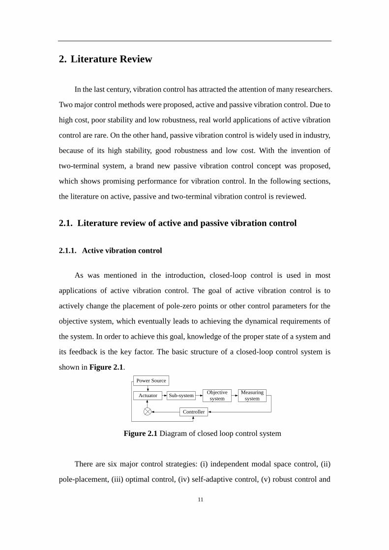
As was mentioned in the introduction, closed-loop control is used in most
applications of active vibration control. The goal of active vibration control is to
actively change the placement of pole-zero points or other control parameters for the
objective system, which eventually leads to achieving the dynamical requirements of
the system. In order to achieve this goal, knowledge of the proper state of a system and
its feedback is the key factor. The basic structure of a closed-loop control system is
shown in Figure 2.1.
Actuator
Power Source
Controller
Measuring
system
Objective
systemSub-system
Figure 2.1 Diagram of closed loop control system
There are six major control strategies: (i) independent modal space control, (ii)
pole-placement, (iii) optimal control, (iv) self-adaptive control, (v) robust control and
12
(vi) intelligent control. Each of them will be briefly reviewed in the following.
2.1.1.1. Independent Modal Space Control (IMSC)
By separating the vibration system into mode sequences, this method focuses on
controlling the active mode to control the whole vibration system [40]. Baz and Poh [41]
proposed an experimental implementation of Modified Independent Modal Space
Control (MIMSC), by using a piezo-electric actuator to control several vibration modes.
Experimental results showed that with maximum modal energy ranking, MIMSC is an
efficient approach to damping the vibration of the objective system.
However, the modes of vibration of a system often cannot be easily calculated due
to the coupling between them. An optimal modal coupling control algorithm usually
presents a large computational burden, even for a supercomputer, which is the main
limitation of this approach to vibration control [42].
2.1.1.2. Pole-placement
This approach includes choosing different eigenvalues and eigenvectors to control
the vibration system. It is well known that system eigenvalues will affect the dynamic
characteristics of the system, and eigenvectors will affect its stability [43–45]. Through
state feedback or output feedback, the location of system poles can be relocated to meet
the criteria of the target system.
Bueno and Zanetta [46] presented a new pole placement method by using the
system matrix transfer function and sparsity, and experimental results indicate that this
method can be applied to different conditions with small signal stability analysis of
large system. However, it is extremely difficult to adjust the pole into a proper location
via a pole placement method in industrial applications due to their complexity [47].
2.1.1.3. Optimal control method
By using mathematical algorithms such as the extremism principle, optimal
filtering and dynamic programming, the theory of optimal control can be used to

13
determine the optimal control input which will meet the system requirements. For
linear systems with a quadratic performance index, the optimal feedback control can be
presented in analytical form. Software for these calculations already exists [48,49].
In the last two decades, optimal control has been applied to many fields[50–52].
For example, constrained layer damping as an effective vibration suppression approach
has been applied to many industrial problems [53–55]. Xie et al.[56] proposed a new
optimal vibration control method for a rotating plate with self-sensing active
constrained layer damping, which demonstrated the potential for more efficient
vibration control. Optimal control has also been used in tracked vehicle suspension
systems, where simulation also demonstrated the possibility for efficient, real-time and
robust control [57]. However, for systems of higher order than two, the determination
of optimal control is complicated, and it is also extremely difficult to present in
analytical form [58].
2.1.1.4. Self-adaptive control
A Self-adaptive control system is one which can automatically monitor the
changing of system parameters, and maintain an optimum system performance index in
real-time [59]. It can be classified into three different types: self-adaptive feed-forward
control, self-correction control and model reference self-adaptive control. When it is
assumed that the disturbance is measurable, self-adaptive feed-forward control can be
applied [60]. Self-correction control integrates real-time identified parameters of a
vibration system with parameters of the actuator, which eventually achieves
self-correction control [61]. The main theory of model reference self-adaptive control is
that the vibration system will be driven by the self-adaptive system, which requires that
the output of a vibration system follow the output of a model reference [62].
Self-adaptive control usually shows high performance for system control, because it
can change the system parameters in real-time.
Valoor et al. applied self-adaptive control method to smart composite beams using
recurrent neural architecture. By developing a finite element model, simulations were
carried out and the results indicated high efficiency and good robustness of the

14
implementation [63]. However, self-adaptive control usually requires a good model of
the vibration system, which may not always be feasible. Additionally, in order to
achieve real-time control, sensors and actuators with high precision are also required,
which implies an increase in the cost of implementing the control system [64].
2.1.1.5. Robust control
Through linear feedback, robust control can provide a certain capacity for resisting
disturbances for a closed-loop system. Although self-adaptive control can also be
applied to a vibration system with uncertainty, there is still a major difference between
the two control approaches. Robust control uses excessive controllers to ensure that the
state of the target system will move to a stable configuration. If the changing rate of
system parameters stays at the design requirements of the controller, this system will
always be stable [65].
Based on robust control, Sun et al. [66] proposed an adaptive robust vibration
control of a full-car active suspensions with electro-hydraulic actuators. By testing on
different road conditions, the high stability of this control system was demonstrated
through a Lyapunov framework. Since robust control requires excessive control, which
inevitably leads to chattering, a decrease in the precision of the system-tracking and
also an increase to the abrasion of the actuator [67].
2.1.1.6. Intelligent control
As one of most popular methods of vibration control, the development of
intelligent control presents a whole new field for active vibration control. Fuzzy control
is a major branch of intelligent control, which provides an effective approach to solve
complicated control system problems[68]. Models of many systems cannot be easily
developed. However, fuzzy control not only provides objective information of the
target system, but can also embed the experiences and intuition of human intelligence
into the control system [69]. Neural network control is another approach to intelligent
control. The neural network based intelligent control uses massively parallel processing
to simulate the structure and function of a human neural network for application to
nonlinear dynamical systems. For some situations, these two methods can also be

15
combined into a fuzzy neural network control approach [70].
Aliki et al. [71] applied fuzzy control to vibration suppression of a smart elastic
rectangular plate. A comparison was carried out between fuzzy control and a more
traditional proportional integral derivative (PID) controller. The results indicated better
vibration suppression with the fuzzy control approach. Another self-learning system
was proposed by Gordon, which has been applied to optimize the vehicle suspension.
This self-learning system can be used for real-time control [72].
Because intelligent control usually requires pre-description of a system function,
this implies that sample data with sufficient precision are necessary. If intelligent
control cannot achieve the control function as predicted, trouble-shooting is usually
difficult [73].
2.1.1.7. Semi-active vibration control
In the last several decades, researchers have been focusing on semi-active
vibration control [74,75]. Semi-active vibration control can be considered as a branch
of passive vibration control, since in many cases there is no direct mechanical energy
input into the control system. However, in order to achieve semi-active vibration
control, a minor outside energy source is needed to control the actuator and actively
adjust semi-active vibration control devices. Moreover, feedback control is applied in
most cases of semi-active vibration control, which makes semi-active vibration control
more similar to active vibration control.
Semi-active vibration control devices are usually combined control systems
consisting of devices with passive stiffness or damping and a mechanical active
actuator [76]. Active variable stiffness systems (AVS) and active variable damping
systems (AVD) are classic examples of semi-active vibration control devices [25,77].
Since the main feature of a semi-active vibration control system is providing an
optimum control force, active control theory is fundamental for semi-active vibration
control. Furthermore, because the control force of a semi-active vibration control
system is limited, the active control algorithm which drives the semi-active vibration
control to output the optimum control force must be related to the semi-active vibration
16
control force. In 1990, the Kajima research center firstly applied the AVS system to a
three-story office building, which resulted in high performance under low or medium
level earthquakes[78]. In 1997, a bridge with an AVD system was first built in America,
which resulted in vibrations caused by heavy-loading vehicles to be effectively
suppressed [79].
The most important application of semi-active vibration control is semi-active
suspensions for vehicles. This theory was proposed by Crosby and Karnopp in 1970s,
but applications started at the beginning of the 1980s [80–82]. Different from a passive
or active suspension, a semi-active suspension system consists of a constant stiffness
spring and variable damping shock absorber, which is also called a no source active
suspension due to the minor energy input. In a semi-active suspension system, there is
no actuator to generate the control force. Instead, the controller calculates the control
force based on data from the sensors and then adjusts the damping of the shock absorber
to produce the needed control force, which in turn finally achieves vibration
suppression [83].
There are three major types of shock absorber used to achieve semi-active
vibration control: hydraulic shock absorber [84], electro-rheological (ER) fluid
vibration damper [85] and magneto-rheological (MR) fluid damper [86]. All these
shock absorbers usually consist of a small accumulator with a damping valve and a
hydraulic control system, which will make the damping force generated by the
hydraulic shock absorber proportional to the absolute velocity of the vehicle. In
particular, the magneto-rheological fluid damper has been widely used in many
vibration systems due to its high damping ratio and low energy cost.
For example, in 1999, Suh and Yeo proposed a theory by using the
Binghan-plastic model of ER fluid to estimate the damping force of an ER fluid damper.
Through this, the main parameters of the ER damper can be accurately determined and
experimental results indicate the actual damping force is in good agreement with the
estimated damping force [87]. With the invention of the MR damper, more and more
researchers have focused on this specific area, in particular for high-mobility

17
multi-purpose wheeled vehicle [88,89]. Karakas et al. used experiments with a quarter
car model to investigate the performance difference between the MR damper and
original equipment manufacturer damper. Through skyhook control algorithms, the
experimental results indicate that the MR damper can help to achieve highly-efficient
vibration suppression [90].
2.1.2. Passive vibration control
As mentioned above, active vibration control usually requires an outside energy
source to generate the force required to suppress vibrations. Due to the high cost and
low reliability of active controllers, industrial application of active vibration control is
limited. On the other hand, passive vibration control due to its associated low cost and
high reliability is widely used for vibration control. Passive vibration control can often
be realized by structural design [91,92] and has been applied to two major fields:
structural vibration control and mechanical passive vibration control.
2.1.2.1. Passive vibration control by structural design
In many mechanical or civil engineering applications, a machine or structure will
experience vibration. If this is known in advance, the vibration level may be effectively
minimized through optimal design. In particular for some customized structures, this
will usually involve calculation, testing, modification, re-calculation and re-testing.
However, with the development of Computer Aided Design (CAD), optimal design of a
structure is much easier. Instead of a manual design process, design and modification of
the prototype can be performed with a computer, and additionally the reliability can
also be analyzed through computer simulation [93].
There are several methods of structural design approaches to achieve passive
vibration control. These are: de-tuning, reducing the number of responding modes,
de-coupling, structure stiffening, optimizing the structural geometry and selecting the
best material, respectively [91,92,94]

18
When there are spectral spikes at certain frequencies in the excitation, the method
of de-tuning can be applied [95]. The basic theory of de-tuning design is that the design
and modification of the structure will eventually avoid the near proximity of the
resonance frequencies and spectral spikes. The approach of reducing the number of
responding modes usually can be applied when the structure is under finite-band
random excitation [96]. Since the total response of the structure depends on the number
of modes, reducing the number of modes results in effective vibration suppression.
De-coupling has been used to describe many procedures, but in structural design,
there are two types of de-coupling which can lead to vibration control. The first one is
de-coupling the different types of motion at the design state, implying that one type of
vibration (e.g. linear) should not excite a different type of vibration (e.g. rotational).
The other one is separating the natural frequencies of different components of a
structure [97]. By de-coupling the natural frequencies, the whole structure will not
resonate under excitation with one fixed frequency.
There are only a few cases of passive vibration control that involve structural
stiffening [98]. This follows because an increase in stiffness of a structure will
inevitably change its natural frequencies, which may lead to resonance frequencies
becoming closer to possible excitation frequencies [99].
When the type of excitation is known, optimization of the structural geometry can
lead to vibration suppression. The last method of vibration suppression by structural
design is through the selection of the best material under different situations. With the
development of material engineering in last several decades, many new compound
materials are being discovered or designed, and these have shown high performance in
suppression of vibration [100].
2.1.2.2. Structural passive vibration control
In vibration control of structures, passive control can be classified into three basic
types: seismic isolation control, energy dissipation control and energy absorption
control [101].

19
Seismic isolation control: By applying an isolation layer at the bottom of the
structure above ground, the structure can be separated from the top surface of the
foundation. In this way, the seismic energy will be blocked from the main structure,
which eventually leads to the reduction in vibrations [102]. Seismic isolation control
usually requires variable horizontal stiffness. Under strong winds or low-level
earthquakes, the displacement of the upper structure can be made to be extremely small
by using a sufficiently high horizontal stiffness [103]. This in turn ensures that the main
structure is not affected. When the earthquake is of medium strength, the upper
structure will lightly slide in the horizontal direction due to the small stiffness, which
will transform the rigid seismic structure into flexible seismic structure. The natural
period of vibration will be obviously extended, and separated from the natural period of
the lower structure and characteristic period of the ground [104]. Through this, the
vibration of the ground can be effectively isolated, which reduces the seismic reaction
of the upper structure.
Seismic isolation control is one of oldest passive vibration control methods, and it
is also the most popular due to its high reliability and straightforward application.
However, this method cannot be applied to high rise buildings or to the control of
vibrations caused by strong winds.
Energy dissipation control: There are two ways to achieve energy dissipation
control [105,106], one is via no-load-bearing components (such as a supporting wall,
shear wall and connector) of the structure that have been designed as energy dissipation
devices. The other approach is through dampers that are located at some specific
locations (such as interbedded space, nodes and connection space) of the structure.
Under the situation of low-level seismic forces or winds, the initial stiffness of the
energy dissipation components is sufficient to make them stay in an elastic state, which
has enough lateral rigidity to satisfy the application requirements of the main
structure[107]. When the earthquake is of a higher magnitude, the energy dissipation
components will stay in an inelastic state, which eventually keeps the main structure

20
and all components from seismic destruction.
Energy dissipation devices can be classified as damping, energy dissipation
supporting device and energy dissipation wall [108]. To be more specific, the dampers
can be listed as a metal damper, friction damper, viscous damper, viscoelastic damper,
composite damper and so forth. For energy dissipation supporting, there are three types
including eccentric energy dissipation supporting, friction energy dissipation
supporting and cycle energy dissipation supporting [109]. The major types of energy
dissipation wall can be summarized as band seam energy dissipation wall, horizontal
seam roof energy dissipation wall and damper energy dissipation wall [110].
Energy absorption control: By adding an additional sub-structure, energy
absorption control will transfer the vibration of the main structure to the sub-structure.
The vibration energy of the main structure will be distributed into the main structure
and sub-structure, which leads to the reduction of vibrations [111,112]. Most of the
extra sub-structures consist of mass, damper and stiffness elements. Through adjusting
these three components, the natural frequency of vibration of the sub-structure can also
be changed. This will be adjusted to be as close as possible to the excitation vibration
frequency of the main structure. When there is excitation of the main structure, the
sub-structure will generate inertia forces with opposite direction of the vibration of the
main structure, which eventually achieves the reduction and control of vibration [113].
The types of energy absorption passive control devices include tuned mass
dampers (TMD) [114], tuned liquid dampers (TLD) [115], pendulum mass
dampers[116], air dampers and hydraulic-mass vibration control systems [117]. Of all
these devices, the TMD is the most widely used in industry [118]. By using the inertia
of the mass, the TMD can increase the damping ratio of the main structure to achieve
vibration control. In order to achieve the best results, TMD is usually located at the
point where the vibration reaches the maximum amplitude. However, modern
architecture adds various equipment or hanging gardens on the top of many buildings,
which often makes the installation of a TMD impossible[119]. In particular, in the case

21
of a television tower, a TMD is impossible to install due to the presence of the satellite
antenna. Finding the optimum location for a TMD is also extremely important for
energy absorption control [120].
2.1.2.3. Mechanical passive vibration control
As mentioned above, the vibration of mechanical systems is a universal
phenomenon. Tremendous progress has been made with vibration control in
mechanical systems. In particular, passive vibration control, due to its low cost, high
reliability and high robustness, has been widely applied in industry [12,91,92]. Within
the realm of passive vibration control, vibration control for rotating systems and vehicle
passive suspension are two major applications of mechanical passive vibration control.
Rotation system passive vibration control: Rotating systems are the most
common device within a mechanical system, and can be found in many industrial
applications [28,121]. Due to manufacturing defects, the centroid of each
micro-segment of a rotor generally has a small deviation from the axis of rotation. Due
to this deviation, centrifugal forces will cause the vibration of the rotor when it is
rotating. The vibration of the rotor will not only cause noise and shorten the service life,
but also in extreme cases will cause the failure of the whole system.
In the past several decades, researchers have been achieving huge progress in
rotating system vibration control [122,123], in particular with respect to reliability, cost,
robustness and simplicity. In general, the vibration of a rotating system can be classified
into four different types: steady-state oscillation, unstable vibration, self-excited
oscillation and torsional vibration. Each of these will be discussed in turn.
Steady-state oscillation: In a rotating system, the static and dynamic balance of
the rotor is extremely important. If the rotor is unbalanced, when the rotation frequency
reaches the natural frequency of the rotor, vibration caused by harmonic resonance will
occur [124]. For this situation, Tatara proposed a bearing with rubber to support the

22
rotor, which can be used for damping by friction [125]. However, for some machines,
e.g., a laundry machine, the unbalance of the rotor changes as the operations change.
Theale proposed an automatic ball balancer, by locating two balls in the cavity with
appropriate angles on the opposite side to the unbalance, which will eventually balance
the rotor automatically in the post-critical speed range [126].
Unstable vibration: In a rotating system, the rotor is usually connected with some
transmission components, such as a shaft. When the geometric structure of this shaft is
asymmetric, unstable vibration will occur if the rotation speed is close to the critical
speed of the rotor. The main strategy for this circumstance is to make dummy slots on
the shaft, which can eliminate the asymmetry [127,128]. In 2010, Ishida and Liu
proposed a method to suppress such an unstable vibration by using discontinuous
spring characteristics [129]. With this method, the range of rotation speeds for unstable
vibration can be adjusted above the major critical speed.
Self-excited oscillation: internal friction or internal damping in a rotating system
are caused by friction between the rotation components, which inevitably leads to
vibration of the system in the post critical speed range [130]. By using leaf springs to
support the outer ring of the bearing that is mounted on the shaft, a new method was
proposed to dissipate energy to suppress the self-excited oscillation. The damping
intensity can be adjusted by changing the preload on the leaf spring [131].
Torsional vibration: The driving torque in multi-cylinder reciprocating engines
changes at certain periods due to complicated processes such as combustion, intake,
exhaust strokes and compression [132,133]. This vibration not only causes problems
for the rotating mechanics system, but also imposes an unhealthy work environment on
the operator of the machinery. Many devices have been invented to suppress torsional
vibration, a centrifugal pendulum vibration absorber being one of the most famous
[134–136]. By using the idea of an anti-resonance point for a two-degree freedom

23
system, this damper can effectively achieve vibration control.
2.1.2.4. Vehicle passive suspension
As mentioned above, vehicle suspension is one of the most successful and popular
applications of passive vibration control. Researchers have been achieving impressive
progress with vehicle passive suspensions in the last several decades. Due to high
reliability, good robustness and low cost, passive suspensions still play a major role in
vehicle vibration control. Most vehicle passive suspensions can be classified into two
different types: non-independent suspension and independent suspension [82,83,137].
Non-independent suspension: The defining structural characteristic of a
non-independent suspension is that both sides of the wheels are connected by a wheel
axle, and that the wheels and wheel axles are suspended under the car body by an elastic
suspension. There are many advantages to a non-independent suspension, namely
simplicity, low cost, high strength, easy maintenance and small changes in the
orientation of the front wheels on the road. However, due to poor ride comfort and
handling stability, this kind of suspension is now mainly used for trucks and buses
instead of passenger cars [138].
There are four kinds of springs for non-independent suspensions [139], leaf spring
[140], coil spring [141], air spring [142] and oil-gas spring. As indicated by their names,
leaf, coil, air and oil-gas spring non-independent suspensions use leaf springs, coil
springs, air springs and oil-gas springs as their elastic components, respectively. The
type of spring used represents the major difference between these non-independent
suspensions [138].
Independent suspension: unlike non-independent suspensions, the defining
structural characteristic of an independent suspension is that each side of the wheel is
individually suspended under the car body through an elastic suspension [142].
Compared to a non-independent suspension, there are four advantages to an

24
independent suspension. First, the reduction in weight reduces the impact on the car
body and increases adhesion between the wheel and the road. Second, a spring of
relatively low stiffness can be used for this suspension, which improves the ride
comfort. Third, the location of the engine can be lower, which leads to a lower center of
gravity of the car and thus increased stability. Lastly, the vibration between the two
sides of the vehicle are uncoupled, which eventually causes a reduction of inclination
and vibration of the vehicle [82,83,143].
Despite the complicated structure, high cost and inconvenient maintenance,
independent suspensions are still the preferred design choice for most modern
passenger vehicles. Independent suspensions can be classified as (i) wishbone
suspension, (ii) multi-link suspension, (iii) trailing arm suspension, (iv) sliding pillar
suspension, and (v) McPherson suspension [144–146].
A wishbone independent suspension implies that the wheels of the car can only
swing in the transverse plane. Wishbone suspensions can be separated into single
wishbone and double wishbone suspensions, according to the number of transversal
arms [147,148]. The application of a single wishbone independent suspension is rare in
modern car design, because this suspension will cause the rear part of the car to swing
when the car is under high speed [149]. Double wishbone independent suspension can
be specified as isometric wishbone or long-short wishbone independent suspension. An
isometric wishbone independent suspension has the same disadvantage of a single
wishbone independent suspension. However, a long-short wishbone independent
suspension can be optimized in the length of the long and short wishbones and the
location of the two wishbones. This suspension can also provide high ride stability
[150–152].
A multi-link independent suspension is a combination of three to five control rods,
which leads to location changes of the wheels. This suspension will make the car turn
smoothly, following the driver‟s intention; however, there will be shaft swing when the
car is running at a high speed [154]. A trailing arm independent suspension is similar to
a wishbone independent suspension, the wheels of the car only swing in the vertical

25
plane. It can also be classified as single and double trailing arm independent suspension.
This suspension is usually applied to a steering wheel [153,154].
The structural characteristic of a sliding pillar independent suspension is that the
wheels are moving up and down along the kingpin axis, which is rigidly fixed to the car
frame. There are only a few applications about this suspension, because the kingpin will
take most of the lateral force during driving, which increases the abrasion of the kingpin
and shortens its service life [155]. The wheels of a McPherson independent suspension
still move along with the kingpin. However, unlike sliding pillar independent
suspensions, the kingpin can swing instead of being rigidly fixed. A McPherson
independent suspension is a combination of a wishbone and sliding pillar independent
suspensions [156]. Compared to wishbone independent suspensions, McPherson
suspensions have a compact structure, small changes of front wheel orientation on the
road and high handling stability [157]. The lateral force on the kingpin is also much
smaller than with a sliding pillar independent suspension. This suspension has been
widely used for medium or small size cars [158]. However, with the advancement of
technology, more attention is paid to the controllability rather than the cost, which is a
challenge for passive vibration control.
2.2. Literature Review of Two-terminal vibration control system
2.2.1. Electrical passive network
The main research on electrical passive networks uses a limited number of
resistors, inductors, capacitors and transformers to describe a function within a given
network. There are two main features of electrical passive networks. First, before an
excitation is applied there are no voltages or currents between any two terminals. The
second feature is that for any arbitrary excitation, there is no negative energy delivery in
the network [159]. In 1931, Brune first defined the electrical passive network and
proved that the resistance or admittance function is a positive-real function for all
passive networks [160]. Brune also proposed a general method named the Brune

26
Comprehensive Method, which is used to describe any positive-real function by using a
limited number of resistors, inductors, capacitors and transformers.
In the past several decades, much research has been done on electrical passive
networks[161,162]. However, the redundancy of components in passive networks is
still the main obstacle to its development. Especially for multi-terminal passive
networks, a non-transformer solution is still impossible[159]. In the 1970s, with the
development of the integrated circuit, interest in research on electrical passive networks
started to wane [163].
2.2.2. Mechanical passive networks
In many industrial mechanical control systems, passive components are applied,
for example, to vehicle suspension systems and mechanical vibration control systems
[164]. Compared to mechanical active networks, passive networks are valued due to
their high reliability and low cost. However, structural design and selection of
components for a mechanical device is extremely complicated and is usually achieved
by trial and error [163].
In order to describe a mechanical system accurately, many researchers attempt to
analogize a mechanical system with an electrical system by using a force–current
analogy [165]. With the analogy of force-current and velocity-voltage, the system
consisting of passive mechanical components can be considered as a passive
mechanical network. In a mechanical system, if all the components can be made to
correspond to resistors, inductors, capacitors and transformers in an electrical system,
the theory of electrical passive network can be applied to the mechanical passive
network. According to the kinetic equation, resistors, inductors and transformers in
electrical systems can be analogized in the mechanical system as dampers, springs and
shafts respectively [142]. The specific analogies between electrical and mechanical
systems are shown in Table 2.1.

27
Table 2.1 Analogy between electrical system and mechanical system [167]
Electrical System Mechanical System
Current (i) Force (F)
Voltage (u) Velocity (v)
Electrical zero point
(Voltage=0)
Mechanical zero point
(Velocity=0)
Resistor (R = resistance)
i i
1u 2u
R
u Ri
Damper (c = damping constant)
F F
1v 2v
c
cv F
Inductor (L = inductance)
i i
1u 2u
L
diu L
dt
Spring (k= stiffness)
F F
1v 2v
k
1 dFv
k dt
Transformer Lever
Capacitor
i i
1u 2u
C
duC i
dt
Mass
F F
1v 2v
m
dvm F
dt
Electrical connectors Mechanical connectors
2.2.3. Two-terminal vibration control system
2.2.3.1. Two-terminal mass system
As mentioned above, the theory of electrical passive networks can be applied to
mechanical passive networks if all the corresponding components are matched.
However, for the analogy between capacitance and mass, the two terminals of the mass
element need to be defined to match the two terminals of the capacitor. According to
Newton‟s second law, one terminal of the mass element is the center of mass, and the

28
other one should be a fixed point in the inertial frame [164]. Therefore, the mass
element is analogous to a grounded capacitor, as shown in Table 2.2.
Table 2.2 Analogy between mass element and grounded capacitor[32]
Capacitor(Grounded)
i
1u 2 0u
C
duC i
dt
Mass(Grounded)
F
1v2 0v
m
dvm F
dt
Based on Table 2.2, the mass element can be analogized as a grounded capacitor.
However, there are still two major problems about this analogue. First, there is the
possibility that unreasonably large masses may be required. Second, if the capacitor is
not grounded, there is no direct mechanical component which can be analogized [168].
2.2.3.2. Two-terminal mass devices
(1) Inerter: In 2002, Smith proposed a new two-terminal mass device named
inerter, which resolves the capacitor analogy difficulty mentioned above [32]. This
inerter can not only be used for analogizing the capacitor in electrical networks, but can
also generate as high as several hundred times equivalent mass even if the real mass
(gravitational) of this system is small [169,170]. The prototype of inerter is shown in
Figure 2.2.
(a)

29
(b)
Figure 2.2 Prototype device: Inerter (a) Prototype of inerter, and (b) schematic of
inerter[171]
(2) Inverse screw two-terminal system: Inverse screw two-terminal system is a
combination of flywheel and inverse screw transmission system [35]. Through the
inverse screw transmission system, the inverse screw two-terminal system can transfer
vertical or horizontal movement into rotation, which eventually leads to the generation
of large equivalent mass. The prototype is shown in Figure 2.3.
(a)
(b)
Figure 2.3 Prototype of inverse screw two-terminal system (a) prototype of
inverse screw two-terminal system, and (b) schematic of inverse screw two-terminal
system [38]

30
(3) Electro-hydraulic variable two-terminal mass device: In 2011, Li and
Liang proposed an electro-hydraulic variable two-terminal mass device, which can
generate variable equivalent mass [37]. By changing the voltage of the electrical valve,
the transmission ratio will also change, which will in turn cause the generation of
different equivalent mass. The prototype of the electro-hydraulic variable two-terminal
mass device is shown in Figure 2.4.
(a)
(b)
Figure 2.4 Prototype of electro-hydraulic variable two-terminal mass device (a)
Prototype of electro-hydraulic variable two-terminal mass device, and (b) schematic of
electro-hydraulic variable two-terminal mass device [37]
All these two-terminal mass devices have been used for vibration control by many
31
researchers [169], [171], [172]. Chen et al. combined the inerter with a conventional
semi-active control system. The experimental results indicated that compared to
traditional semi-active control, semi-active control with inerter has shown better
vibration suppression performance [172]. Li and Liang also applied a two-terminal
hydraulic system to a vehicle suspension [36]. Compared to conventional passive
suspension, this two-terminal hydraulic system demonstrated better performance on
passenger comfort and tire grip [36]. However, most of these two-terminal mass
vibration control systems can only generate constant equivalent mass, because the
moment of inertia of the flywheel is constant. Even if they can generate variable
equivalent mass, this usually requires a complicated structure and associated high cost.
Moreover, a flywheel with fixed moment of inertia will also add more weight to a car,
which means more energy consumption.

32
3. Design and theoretical analysis of nonlinear two-terminal
mass mechanisms
In this chapter, two different adaptive flywheel designs are proposed, and the
corresponding mathematical models for the adaptive flywheels are derived. The first
proposed flywheel is made of metal and the second is made of nylon. Compared to the
metal adaptive flywheel, the nylon adaptive flywheel can generate less equivalent
mass, but the changing ratio of the nylon adaptive flywheel is much higher. To
analyze these adaptive flywheels, a two-terminal hydraulic device and a two-terminal
inverse screw device are introduced. The mathematical models for both two-terminal
devices are also derived. At the end of this chapter, the design strategy for an adaptive
flywheel is discussed. The reasons for choosing certain specific parameters for the
adaptive flywheel are illustrated.
3.1. Design motivation and proposed designs
3.1.1. Design motivation
As mentioned in the literature review, researchers have been making progress
with vibration control, particularly in structural and mechanical vibration control.
Active and semi-active vibration controls have attracted much attention in the last few
decades. However, due to high cost, low reliability and robustness, real-world
implementations of active and semi-active vibration control are still rare. Passive
vibration control still dominates industrial applications because of low cost, high
robustness and high reliability. However, in the case of passive vibration control, once
key system parameters (stiffness, damping ratio and mass) have been chosen, the
characteristics of the system are then fixed. This implies that the ability of a passive
vibration control system to deal with a variety of situations is limited. Therefore, the
design must always make compromises, favoring the conditions that the passive system

33
is most likely to encounter at the expense of other conditions which are expected to
occur less frequently.
With the invention of the inerter, there was increased interest in two-terminal mass
vibration control [36,173] - a new and effective method of passive vibration control. By
achieving a much larger equivalent mass through the flywheel in the system, a
two-terminal mass vibration control system can change the natural frequency of the
whole system, which in turn can lead to the suppression of vibrations. However, most
of these two-terminal mass vibration control systems can only generate a constant
equivalent mass. The generation of variable equivalent mass would make it possible to
change system parameters „on the fly‟. However, as mentioned earlier, this usually
requires complicated mechanisms at high cost. Moreover, the flywheel would also
cause an increase in the overall weight of the system, which implies higher energy
consumption.
3.1.2. Proposed designs
For all the reasons mentioned above, a new type of adaptive two-terminal mass
system is therefore proposed in this thesis. In place of a constant flywheel fixed on a
two-terminal mass system, a new type of adaptive flywheel will be added and evaluated.
There are three features of this new adaptive flywheel that are pertinent. First, the
proposed adaptive flywheel can generate the same equivalent mass as a traditional
non-adaptive flywheel, but with less weight. Second, this flywheel can passively
generate different equivalent mass, and the change in equivalent mass is large enough
to be significant. Finally, with the adaptive flywheel, the whole two-terminal vibration
control system exhibits nonlinearity in vibration control. Compared to a linear vibration
control system, a nonlinear system may offer a better ability to suppress vibrations
[174–176].
Since the intended application of the proposed adaptive flywheel is mainly for
vehicle suspension systems, there are two design requirements that need to be satisfied.

34
First, the size of the flywheel must be small enough to fit into the vehicle suspension
system rattle space. Second, three performance criteria must be considered for the new
adaptive two-terminal mass system: passenger comfort, tire grip and suspension
deflection.
Two adaptive flywheels with different materials are proposed, designed and
manufactured. Subsequent to the designs of the new adaptive flywheel, two traditional
two-terminal systems (i.e., the two-terminal hydraulic transmission system and the
two-terminal inverse screw transmission system) connected to the new adaptive
flywheels are also proposed and analyzed. Mathematical models of the two different
two-terminal systems with adaptive flywheels will also be developed in the thesis.
3.2. Theoretical analysis for two-terminal hydraulic device with
metal adaptive flywheel
3.2.1. Mathematical calculation of metal adaptive flywheel
Om
rm
Rm
Pmlm
am
3
1
5
2
4
(a) (b)
Figure 3.1 The metal adaptive flywheel: a) schematic diagram, and b) prototype
(note: 1-spring, 2-inner hole for the shaft, 3-slot, 4-slider, and 5-frame)

35
The prototype of the metal adaptive flywheel is shown in Figure 3.1. There are
four slots in the circular plate. In each slot, there is a slider and spring. The rotation of
the flywheel will cause slider motion along the slot. The moving sliders will compress
the springs to a certain extent, depending on the rotational speed of the flywheel. The
variable location of the sliders in the slot leads to variable moment of inertia of the
flywheel. The parameters of this prototype are shown in Table 3.1.
Om
Pmlm
Figure 3.2 Slot of the metal adaptive flywheel
To analyze the variation in the moment of inertia of the metal adaptive flywheel,
consider one slot shown in Figure 3.2. Point Om in the figure is the rotation center of
the flywheel, point Pm is the centroid of a slider, and lm is the distance between the
rotation center of the flywheel and the centroid of the slider. Denote the mass,
diameter, and length of the slider as smm , dm and lsm, respectively. The moment of
inertia of the slider can then be calculated as:
2 2 21 3
12 4szm sm m sm sm mI m d l m l
(3.1)
Equation (3.1) indicates that the moment of inertia of the slider varies with the
distance between the rotation center of the flywheel and the centroid of the slider. In
this equation, the moment of inertia of the spring is neglected due to its relatively
small weight. To maximize the range in the variation of the moment of inertia of the
flywheel, the weights of the frame and other support components should be as light as
possible. In an ideal case, if the weights of the frame and other support components are

36
negligible, and the distance lm is much larger than diameter dm and length lsm, then the
moment of inertia of the metal adaptive flywheel afmI can be written as
24 4afm szm sm mI I m l (3.2)
Equation (3.2) shows that in the ideal case, the moment of inertia of the adaptive
flywheel afmI depends on the distance between the rotation center of the flywheel and
the centroid of the slider.
Table 3.1 Parameters of the metal adaptive flywheel prototype
No Name Notation Specification
1 Radius of inner hole rm 0.01 m
2 Outer radius of the flywheel Rm 0.047 m
3 Length of slot am 0.03 m
4 Width of slot /Diameter of slider dm 0.02 m
5 Length of slider lsm 0.015 m
6 Stiffness of spring ksm 90 N/m
7 Mass of slider msm 0.035 kg
8 Mass of flywheel (including
slots)
mfm 1 kg
9 Mass of the removed slot
material
mom 0.079 kg
Parameters in Table 3.1 will be discussed at end of this chapter. To model the
proposed variable flywheel, its moment of inertia must be calculated. The schematic
diagram of the variable flywheel is shown in Figure 3.1(a). The moment of inertia of
the variable flywheel is given by
4 4afm fzm ozm szmI I I I (3.3)
where Ifzm , Iozm, and Iszm are the moments of inertia of the circular disk (before removal
of the slot), the removed slot material, and one slider, respectively. The moment of

37
inertia of the solid circular disk fzmI (including the slot material) is given by
2 21( )
2fzm fm m mI m r R (3.4)
where fmm is the mass of flywheel (including slots), mr is the radius of inner hole and
mR is the outer radius of the flywheel. As the distance between the rotation center of the
flywheel and the centroid of a slot is given by1
2m mR a , the moment of inertia of one
slot, ozmI , can be obtained from
2
2 21 1
12 2ozm om m m om m mI m d a m R a
(3.5)
where omm is the mass of the removed slot material. The moment of inertia of one
slider szmI can be obtained from Equation (3.1).
Based on the data in Table 3.1, the moment of inertia of the adaptive flywheel
assembly is
4 2 2(8.83 10 0.14 ) .afm mI l kg m (3.6)
Since the travel of the slider is in the range of [0.0225m, 0.0375m], the minimum
and maximum moment of inertia can be calculated as 4 2
,min 9.54 10 .afmI kg m and
3 2
,max 1.08 10 .afmI kg m . The range of the moment of inertia is therefore from
,max ,max ,max( ) /afm afm afmI I I to ,max ,min ,max( ) /afm afm afmI I I , or equivalently 0% to 11.67%,
for this particular prototype.
3.2.2. Relationship between flywheel angular velocity and slider location
Figure 3.1(a) shows that the distance lm between the slider centroid and the center
of the flywheel depends on the acceleration of the slider. The direction of acceleration is
along the slot either toward or away from the rotational center. The acceleration of the
slider is mainly caused by the rotation of the flywheel. This can be represented
mathematically as

38
,min( )sm sm sm m mm a k l l (3.7)
where sma is the radial acceleration caused by rotation, ,minml is the minimum travel of
the slider and smk represents the stiffness of spring. As is shown in equation (3.7), the
friction between sliders and slots is neglected. The sliders and slots have been polished
during the process of manufacture, and surfaces of both sliders and slots are covered
with lubricant oil. Therefore, the friction between sliders and slots is small enough to be
neglected. Since 2
sm m ma l , where m is the rotation speed of flywheel, equation (3.7)
can be rewritten as
2
,min( )sm m m sm m mm l k l l (3.8)
Therefore, it follows that
,min
2
sm m
m
sm sm m
k ll
k m
(3.9)
In our design, the minimum and maximum travel distances of the sliders are
respectively 0.0225 m and 0.0375 m. Hence, the relationship between flywheel slider
angular velocity and slider location can be plotted as shown in Figure 3.3. It should be
noted that according to equation (3.7), lm can theoretically be infinity when
2
sm sm mk m . However, the actual maximum travel of lm is limited to 0.0375 m
because of the outer ring restriction in the design. Therefore, even if the angular
velocity exceeds a certain limit, the slider will remain 0.0375 m from the rotational
center no matter how much faster the flywheel rotates and hence there will be no further
increase in the equivalent inertial mass.

39
0 5 10 15 20 25 30 35
0.025
0.03
0.035
Dis
tan
ce l
m (
m)
Angular Velocity ωm (rad/s)
0.0225
Figure 3.3 The relationship between flywheel angular velocity and slider
location
From Figure 3.3, the relationship between flywheel angular velocity and slider
location is shown, which also indicates the relationship between the angular velocity
and the moment of inertia of the flywheel. When the angular speed is zero, the distance
between rotation center and centroid of slider, lm, is minimum, which means the
moment inertia of flywheel is also minimum. The increase in angular velocity will lead
to increased lm, and hence the increased moment of inertia. However, when the angular
velocity reaches 32 rad/s, lm also reaches its maximum value. Further increasing the
angular velocity will not cause additional increase of the distance between the
rotational center and centroid of slider, and thus the moment of inertia will not further
increase either because the slider has reached the end wall of the slot.
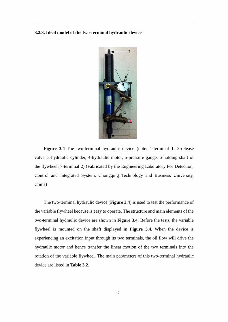
40
3.2.3. Ideal model of the two-terminal hydraulic device
1
2
3
4
5 6
7
Figure 3.4 The two-terminal hydraulic device (note: 1-terminal 1, 2-release
valve, 3-hydraulic cylinder, 4-hydraulic motor, 5-pressure gauge, 6-holding shaft of
the flywheel, 7-terminal 2) (Fabricated by the Engineering Laboratory For Detection,
Control and Integrated System, Chongqing Technology and Business University,
China)
The two-terminal hydraulic device (Figure 3.4) is used to test the performance of
the variable flywheel because is easy to operate. The structure and main elements of the
two-terminal hydraulic device are shown in Figure 3.4. Before the tests, the variable
flywheel is mounted on the shaft displayed in Figure 3.4. When the device is
experiencing an excitation input through its two terminals, the oil flow will drive the
hydraulic motor and hence transfer the linear motion of the two terminals into the
rotation of the variable flywheel. The main parameters of this two-terminal hydraulic
device are listed in Table 3.2.
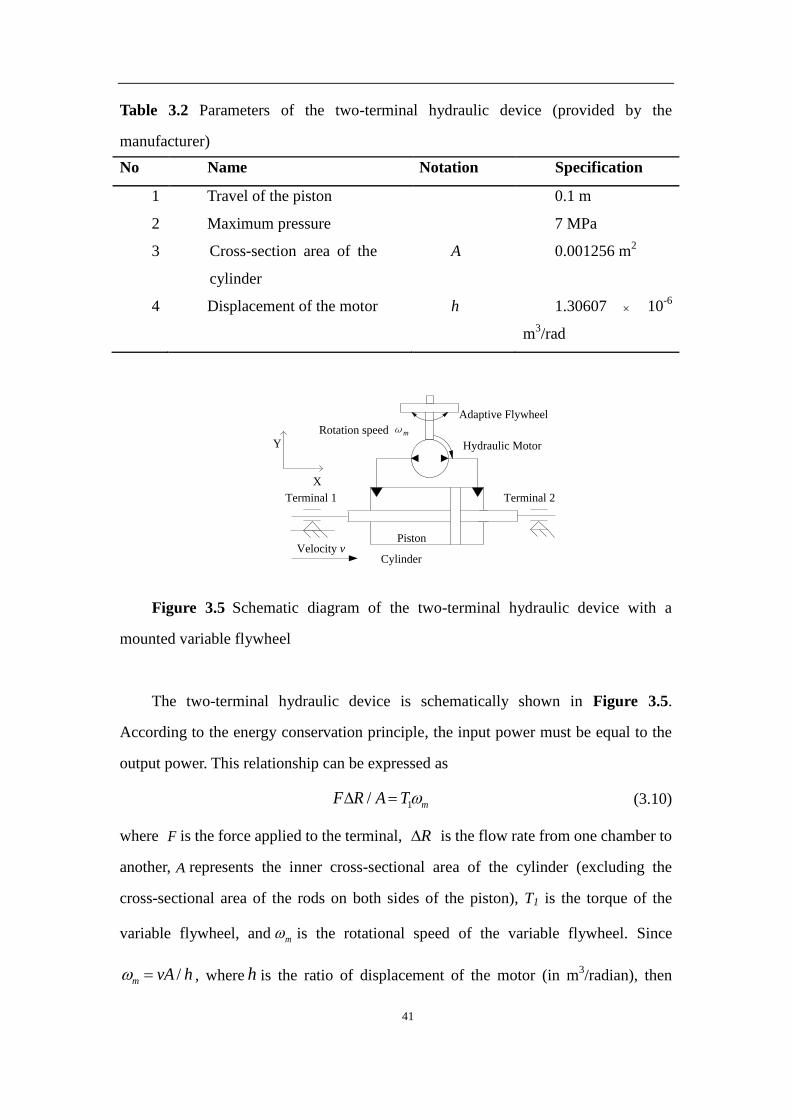
41
Table 3.2 Parameters of the two-terminal hydraulic device (provided by the
manufacturer)
No Name Notation Specification
1 Travel of the piston 0.1 m
2 Maximum pressure 7 MPa
3 Cross-section area of the
cylinder
A 0.001256 m2
4 Displacement of the motor h 1.30607 10-6
m3/rad
Adaptive Flywheel
Cylinder
Terminal 1 Terminal 2
Piston
Hydraulic Motor
X
Y
Rotation speed ωm
Velocity vPiston
Figure 3.5 Schematic diagram of the two-terminal hydraulic device with a
mounted variable flywheel
The two-terminal hydraulic device is schematically shown in Figure 3.5.
According to the energy conservation principle, the input power must be equal to the
output power. This relationship can be expressed as
1/ mF R A T (3.10)
where F is the force applied to the terminal, R is the flow rate from one chamber to
another, A represents the inner cross-sectional area of the cylinder (excluding the
cross-sectional area of the rods on both sides of the piston), T1 is the torque of the
variable flywheel, and m is the rotational speed of the variable flywheel. Since
/m vA h , where h is the ratio of displacement of the motor (in m3/radian), then

42
mR h and 1 afm mT I , equation (3.10) can be rewritten as:
2
2afm
AF I v
h (3.11)
where afmI is the moment of inertia of the variable flywheel. Based on Equation (3.11),
the equivalent inertia mass of the variable flywheel can be calculated by:
2
2em afm
Am I
h (3.12)
3.2.4. Mathematical model of the two-terminal hydraulic system
In the mathematical modeling of this system, four factors will affect this prototype.
These are (i) the oil pressure loss lP in the system (including any leak between the two
chambers and friction of the oil with pipe and cylinder), (ii) the friction fhF between
piston and cylinder, (iii) the stiffness kh of this system, and (iv) the compressibility of
the hydraulic oil. The compressibility of the hydraulic oil under laminar flow used in
this research is 1.023×10⁻⁷
/Pa, which means that a pressure of 6.895MPa can only
cause a 0.5% oil volume change. Hence, this hydraulic oil can be considered as
incompressible. The model of the system can therefore be expressed as:
em l fh h kF m v PA F k x (3.13)
where hk is the stiffness of the system, and kx is the elastic deformation of the system.
The relationship between pressure loss and flow rate can be formulated as:
l hP b R (3.14)
where hb is a pressure loss coefficient. Since mR h and /m vA h , the pressure
loss can be obtained from l hP b vA and the associated reduction in force by
2
l hF b vA . In this hydraulic system, the pressure loss lP can be transferred into energy
loss. In a mechanical system, this can be modeled by an equivalent damper with a
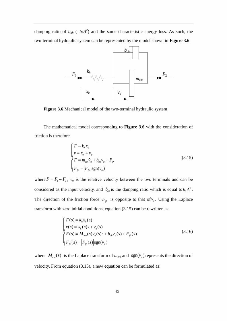
43
damping ratio of bah (=bhA2) and the same characteristic energy loss. As such, the
two-terminal hydraulic system can be represented by the model shown in Figure 3.6.
mem
kh
bah
F1 F2
xk va
Figure 3.6 Mechanical model of the two-terminal hydraulic system
The mathematical model corresponding to Figure 3.6 with the consideration of
friction is therefore
sgn( )
h k
k a
em a ah a fh
fh fh a
F k x
v x v
F m v b v F
F F v
(3.15)
where 1 2F F F , va is the relative velocity between the two terminals and can be
considered as the input velocity, and ahb is the damping ratio which is equal to 2
hb A .
The direction of the friction force fhF is opposite to that of av . Using the Laplace
transform with zero initial conditions, equation (3.15) can be rewritten as:
( ) ( )
( ) ( ) ( )
( ) ( ) ( ) ( ) ( )
( ) ( ) sgn( )
h k
k a
em a ah a fh
fh fh a
F s k x s
v s x s s v s
F s M s v s s b v s F s
F s F s v
(3.16)
where ( )emM s is the Laplace transform of mem and sgn( )av represents the direction of
velocity. From equation (3.15), a new equation can be formulated as:

44
2
2
1( ) ( ) ( ) ( ) ( ) ( )
( ) ( )( )
fh h em ah em ah
h
fh fh
em ah
h h
F s F s k M s s b s M s v s s b v sk
F s F sM s s b s
k k
(3.17)
For this system, the stiffness h fhk F . Therefore, 2
( ) ( )( ) 0
fh fh
em ah
h h
F s F sM s s b s
k k .
To analyze this system, ( ) ( )fhF s F s will be considered to be the output signal, and
( )v s to be the input signal. As mem is a nonlinear function of time t, one cannot obtain a
closed-form expression of the transfer function based on equation (3.17). Therefore, the
transfer function is simply written as follows:
2
( ) ( ) ( )( )
( )
fh h em ah
h em ah
F s F s k m s bG s
v s k m s b s
(3.18)
Equations (3.17) and (3.18) clearly show that the transfer function and hence the
system behavior are affected by four parameters, i.e., bah, Ffh, kh and mem. To examine
the performance of the system, parameters bah, Ffh, and kh will be experimentally
identified and mem will be calculated using equation (3.12), as described in other chapter.
It should be noted that the purpose of presenting equation (3.18) is to show that the
system behavior is affected by the above-mentioned four parameters, but not to find a
mathematical solution.
3.3. Theoretical analysis for two-terminal hydraulic device with
nylon adaptive flywheel
As mentioned in equation (3.2), if the weights of the frame and other support
components are negligible, and the distance lm is much larger than diameter dm and
length lsm, then the moment of inertia of the metal adaptive flywheel afmI will only
depend on the distance lm. However, this is only the ideal condition. In real applications,
the proposed metal adaptive flywheel, the maximum changing ratio defined as

45
,max ,min ,max( ) /afm afm afmI I I is 11.67%. While this changing ratio is likely to be
sufficient for some applications, it is anticipated that larger changing ratios may also be
required for other applications.
In order to achieve a higher changing ratio, another structure design and
materials are required. In last several decades, due to its light weight and high strength,
nylon materials have been widely using in industry of manufacture, which is also ideal
materials for a new design.
3.3.1. Design of nylon adaptive flywheel
In view of the physical strength of the adaptive flywheel and the manufacturing
properties of nylon materials, the schematic diagram of a proposed nylon adaptive
flywheel is shown in Figure 3.7. The flywheel can be fixed on a rotation shaft through
the inner circle. Four drilled slots are evenly distributed in the nylon disk, which are
polished after drilling. In this way, the friction forces between sliders and slots can be
neglected.
Rn
r2n
r1n
Ln
l1n
ln
C
C C-C
dnd1n
Figure 3.7 Schematic diagram of nylon adaptive flywheel (top view and side
view without springs and sliders)
It is well known that the moment of inertia of an object will change with the

46
distance between the object and the center of rotation. Four circular holes are evenly
located near the edge of the nylon disk to further reduce the moment of inertia of the
flywheel. Due to the small moment of inertia of the flywheel, the changing ratio of
moment of inertia caused by the change in position of the sliders will be higher.
A slider and a spring are located in each slot. The centrifugal force caused by the
rotation of the flywheel will drive the slider to compress the spring, where the extent of
the spring compression depends on the rotational speed of the flywheel. The changing
location of the sliders in their slot eventually leads to a variable moment of inertia of the
flywheel.
3.3.2. Moment of inertia of the nylon adaptive flywheel
As shown in Figure 3.7, the total moment of inertia of the flywheel is divided into
four parts: nylon disk (with 4 slots and 4 holes), slots (removed material), sliders and
holes (removed material). The moment of inertia of the springs is neglected because of
their light weight. The density of polyamide 66 is used for calculating the mass of the
slots and holes. The moment inertia of the nylon disc fnI can be represented as
2 2
1
1( )
2fn fn n nI m R r (3.19)
where the mfn is the mass of the nylon disc, Rn is its outer radius and r1n is its inner
radius. For a flywheel of thickness Tn, and density ρ, the mass of the flywheel can be
determined from the density of polyamide 66 as
2 2
1( )fn n n nm R r T (3.20)
Based on the same method, the mass of each slot, onm , and the moment inertia of the
slots, onI , can be calculated as

47
2
11
2
2 2
1 1 1
4
1 3 14
3 4 2
non n
on on n n on n n
dm l
I m d l m R l
(3.21)
where d1n and l1n are the width and length of each slot. The mass of each hole hnm and
the moment of inertia of each hole hnI are presented
2
2
2 2
22 4
hn n n
hn hn n hn n
m r T
I m r m L
(3.22)
where r2n is the radius of each hole, and Ln is the distance of the center of the hole from
the axis of rotation. The mass of the slider, msn, is measured with an electrical scale, and
the moment of inertia of each slider is then calculated as
2 2 2
3 2(3 ) 43
snsn n n sn n
mI r l m l (3.23)
where ln is the distance between the centroid of each slider and the rotation center, 2nl is
the length of slider and 3nr is the radius of slider. By calculating the moment of inertia
of the four parts separately, the total moment of inertia of the flywheel afnI can be
written as
afn fn on hn snI I I I I (3.24)
Table 3.3 Specific parameters of the nylon adaptive flywheel
Name Notation Specification
Outer radius of flywheel
Thickness of nylon disk
Rn
Tn
0.05m
0.022m
Distance between hole and rotation center Ln 0.0375m
Radius of inner circle r1n 0.01m
Radius of holes in flywheel r2n 0.0085m
Diameter of slots in flywheel d1n 0.017m

48
Length of slots l1n 0.035m
Radius of sliders
Length of sliders
Mass of slider
Density of PA66
Stiffness of spring
r3n
l2n
msn
ρ
ksn
0.008m
0.015m
0.0237kg
1150kg/m3
120N/m
The specific parameters for the flywheel are shown in Table 3.3 (these parameters
will be further discussed at the end of this chapter), from which the accurate moment
inertia of the adaptive flywheel can be calculated as
4 2 2(1.75 10 0.0948 ) .afn nI l kg m (3.25)
As shown in Equation (3.25), the moment of inertia of the adaptive flywheel is a
function of variable ln, which implies that the moment of inertia is determined by the
distance between the centroid of the sliders and the rotation center. In this design, the
travel distance of the sliders ranges from 0.0225m to 0.038m, after taking into
consideration that the springs still occupy some space after full compression. The
corresponding maximum and minimum moment of inertia are therefore
4 2
,max 3.12 10 .afnI kg m and 4 2
,min 2.231 10 .afnI kg m , respectively. The range of
the moment of inertia is therefore from ,max ,max ,max( ) /afn afn afnI I I to
,max ,min ,max( ) /afn afn afnI I I , or equivalently 0% to 28.5%, for this particular prototype.
This range is much wider than that of the metal flywheel (i.e., 0% to 11.67%), as
discussed in section 3.2.1.
The relationship between ln and afnI is shown in Figure 3.8.

49
0.024 0.026 0.028 0.03 0.032 0.034 0.036 0.038
2.4
2.6
2.8
3
3.2x 10
-4
Distance (m)M
om
ent
of
Iner
tia
(kg
.m.2)
Figure 3.8 The relationship between ln and afnI
3.3.3. The mechanism of the inverse screw system
As mentioned in section 3.3.2, the changing ratio of the nylon adaptive flywheel is
28.5%, which is much higher than for the metal adaptive flywheel, which has a
changing ratio of 11.67%. However, due to the light weight of nylon material, the
maximum moment of inertia of the nylon adaptive flywheel is much less than the
maximum moment of inertia of the metal adaptive flywheel. If the same two-terminal
hydraulic system is applied to analyze this nylon adaptive flywheel, the equivalent
mass will be much smaller than for the metal adaptive flywheel, which will eventually
lead to an insufficient inertial force in future applications.
Terminal 1 Terminal 2
Nylon Adaptive
Flywheel
Screw
Figure 3.9 Inverse screw system with adaptive nylon flywheel (fabricated by the
Engineering Laboratory For Detection, Control and Integrated System, Chongqing
Technology and Business University, China)
Therefore, a new two-terminal device needs to be applied. In order to achieve
higher equivalent mass and to analyze the characteristics of the nylon adaptive flywheel,

50
it is fixed onto an inverse screw system, as shown in Figure 3.9. If one of the
terminals is fixed, application of an input to the other terminal results in the
transformation of vertical movement into rotation by the inverse screw.
F 1
F 2
x
θd
α
Figure 3.10 Structural diagram of the inverse screw [173]
The structural diagram of the inverse screw is presented in Figure 3.10. The
transmission relationship between vertical acceleration and angular acceleration is
given by [173]
2
tan
x
d
(3.26)
where x is the vertical acceleration, d is the diameter of the ball screw, is the helix
angle of the ball screw, and is the angular acceleration of the flywheel. Based on
Newton‟s laws of motion, the torque on the ball screw should be equal to the torque on
the nylon adaptive flywheel, which leads to [173]
tan
2afn
FdI
(3.27)
where afnI is the moment inertia of adaptive flywheel, and F is the axial force.
Combining equation (3.26) with (3.27), the axial force is calculated as [173]
22
tanafnF I x
d
(3.28)
According to Newton‟s second Law, enF m x , where enm represents the
equivalent mass generated by the nylon flywheel, therefore the equivalent mass enm is

51
given by
22
tanen afnm I
d
(3.29)
From equation (3.25), it is clear that the moment of inertia of the adaptive flywheel, afnI ,
is determined by the distance between the centroid of the sliders and the rotation center,
ln. Assuming that the flywheel is rotating in Figure 3.7, the centrifugal force can be
written as
2
c sn nF m l (3.30)
where cF is the centrifugal force, snm is the mass of the slider, nl is the distance
between the centroid of each slider and the rotation center, is the angular velocity of
the flywheel. The centrifugal force can also be described by the stiffness of spring snk
as
,min( )c sn n nF k l l (3.31)
where ,minnl is the minimum distance between the centroid of the slider and the rotation
center. From the above two equations, the distance ln can be represented by both the
angular velocity of the flywheel and the stiffness of the spring. Combining equations
(3.26), (3.30) and (3.31), the relationship between distance ln and the other variables is
given by
2 2
0.0225
4 / ( tan )
snn
sn sn
kl
k m x d
(3.32)
Furthermore, by combination of equations (3.25), (3.29) and (3.32), the equivalent
mass enm is given by

52
2 2
4
2 2
0.0225 21.75 10 0.0948
4 / ( tan ) tan
snen
sn sn
km
k m x d d
(3.33)
The key specifications of the inverse screw system are shown in Table 3.4.
Table 3.4 Parameters of the inverse screw system (provided by manufacturer)
Name Notation Specification
Diameter of ball screw d 16mm
Helix angle of ball screw 14o
Maximum working travel
distance
-35mm~35mm
3.3.4. Mathematical model of the inverse screw system with nylon adaptive
flywheel
In section 3.3.1, the inverse screw system was shown to lead to the creation of an
equivalent mass enm which is much larger than the mass of the original nylon flywheel.
In achieving an accurate dynamic model of the inverse screw system with the nylon
adaptive flywheel, there are a few factors which should be taken into account.
Since the inverse screw system is based on a screw transmission mechanism, the
backlash problem is a factor which cannot be ignored [173]. The existence of backlash
will affect the transmission precision of a system. However, in some circumstances
backlash will also reduce friction and increase the service life of the transmission
system. In practical applications, there is always the presence of backlash due to many
reasons, such as manufacturing error and thermal expansion.

53
Terminal 2
Flywheel
F1F2
fi
ρ1 ρ2
ciki
x2x1
Terminal 1
Figure 3.11 Schematic diagram of inverse screw system
As shown in Figure 3.11, the transmission path through terminal 1 to terminal 2 is
a screw and bearing path, which is the reason why there are two backlashes 1 and
2 , respectively. The elastic effect in this inverse screw system is another factor which
needs to be considered. The force F(t) which corresponds to the deformation can be
represented as
1 2 1 2( ) ( ) ( )i iF t k x x c x x (3.34)
where ki and ci are the stiffness and viscous damping coefficient respectively, and
1 2x x is the elastic deformation of the system. Under most of circumstances, the
friction of a screw transmission system is negligible considering the large applied force.
In obtaining a more accurate model, the friction fi(t) has also been taken into account as
1 2
1 2
1 2
0
( ) 0 0
0
i
i
i
f x x
f t x x
f x x
(3.35)
Three different situations regarding friction are expressed in equation (3.35). If the
vertical displacement 1x is a positive value (positive direction taken to the right), the
direction of the friction force will be negative, and vice versa. In view of all these
factors, the dynamic model can be developed as given in Figure 3.12.
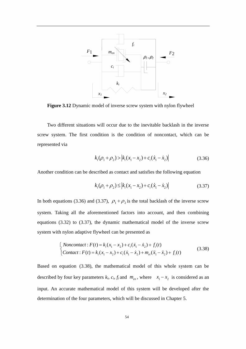
54
ci
fi
ki
men F2F1
ρ1+ρ2
x1 x2
Figure 3.12 Dynamic model of inverse screw system with nylon flywheel
Two different situations will occur due to the inevitable backlash in the inverse
screw system. The first condition is the condition of noncontact, which can be
represented via
1 2 1 2 1 2( ) ( ) ( )i i ik k x x c x x (3.36)
Another condition can be described as contact and satisfies the following equation
1 2 1 2 1 2( ) ( ) ( )i i ik k x x c x x (3.37)
In both equations (3.36) and (3.37), 1 2 is the total backlash of the inverse screw
system. Taking all the aforementioned factors into account, and then combining
equations (3.32) to (3.37), the dynamic mathematical model of the inverse screw
system with nylon adaptive flywheel can be presented as
1 2 1 2
1 2 1 2 1 2
: ( ) ( ) ( ) ( )
: ( ) ( ) ( ) ( ) ( )
i i i
i i ei i
Noncontact F t k x x c x x f t
Contact F t k x x c x x m x x f t
(3.38)
Based on equation (3.38), the mathematical model of this whole system can be
described by four key parameters ki, ci, fi and enm , where 1 2x x is considered as an
input. An accurate mathematical model of this system will be developed after the
determination of the four parameters, which will be discussed in Chapter 5.

55
3.4. Design strategy
3.4.1. The design of the metal adaptive flywheel
As mentioned in section 3.2.1, in an ideal case the moment of inertia of the metal
adaptive flywheel afmI only depends on the distance between the rotation center of the
flywheel and the centroid of the slider, in addition to the weight of the slider. However,
in real applications, many factors need to be considered during the process of design.
Due to the different applications, the actual size of the adaptive flywheel should
also be variable. In our proposed design, the major application of this adaptive flywheel
is a car suspension, which implies that the size of this adaptive flywheel will need to be
small due to the limited space in the suspension system of a car. According to Xu, Smith,
and Li et al [39, 171,173], the outer radius of this flywheel Rm has been eventually
chosen as 0.047m. Due to inner hole, the adaptive flywheel can be mounted on different
devices, which means the radius of this inner hole is determined by the experimental
device. In our design, the radius of the inner hole rm is 0.005m.
Due to physical size and material strength, the size of slots should also be
constrained. Larger size of the slots indicates that additional material will be removed
from the flywheel, but the physical strength of the flywheel will also be reduced.
Considering the reliability and physical size, the length am and the width dm of the slots
are chosen as 0.03m and 0.02m respectively [39].
Based on equation (3.2), the higher weight of the sliders leads to a larger moment
of inertia for the adaptive flywheel. However, due to the heavy weight of the sliders, the
length of the slider will also increase, leading to a shorter travel distance for the slider.
Combining all the factors, the length of slider lsm is chosen as 0.015m [39].
3.4.2. The design of the spring
As mentioned before, different rotational speeds of the adaptive flywheel will

56
drive the sliders to different locations in the slots. However, other than the rotational
speed of the adaptive flywheel, the location of the sliders also depends on the stiffness
smk of the springs. In order to observe the behavior of the metal adaptive flywheel, an
appropriate stiffness smk of the springs needs to be chosen based on experimental
input. During the experiments, if the stiffness smk is too small, the sliders will reach
the maximum stroke under an input with a small amplitude and frequency. On the
other hand, with a high stiffness smk , the sliders cannot reach the maximum stroke
even if under an input with maximum amplitude and frequency. Therefore, an
appropriate stiffness smk will keep the sliders travel under maximum stroke with
most inputs except those with high amplitude and frequency.
From equation (3.9), when the sliders reach the maximum stroke, the relationship
between inputs and stiffness k can be rewritten as:
2
,max
,max ,min
m sm m
sm
m m
l mk
l l
(3.39)
Since /m vA h , it follows that:
2 2
,max
2
,max ,min
m sm
sm
m m
l m v Ak
l l h
(3.40)
Based on equation (3.40), with a given input, the stiffness smk can be determined. In
our experiments, a sinusoidal input with amplitude 1.854m/s is chosen. From equation
(3.40), the value of stiffness smk can be calculated as 90 N/m, which will keep the
sliders travel under maximum stroke with most inputs.
According to the Popov‟s formula [142], the stiffness of spring smk can be
presented as
4
8( )
ssm
m s
Gdk
d d n
(3.41)

57
where md is the diameter of spring, sd is the diameter of the spring wire, G
represents the shear modulus of the material, n is the total circles of the spring. Since
the material of the springs is steel, the shear modulus of the material G should be 83
GPa. However, there are still two unknown parameters G and n in equation (3.41).
As shown in Figure 3.1 (a), the length of the spring should be the length of slot minus
the length of slider, m sma l , which is 0.015m based on Table 3.1. Because of this, a
reasonable assumption of the value of n can be made, which is 4. According to
equation (3.41), the diameter of the spring md can be determined as 0.00051m.
3.5. Conclusion
Two different adaptive flywheels have been proposed, and the corresponding
mathematical models for the adaptive flywheels have also been developed. According
to the mathematical models, the metal adaptive flywheel can generate more equivalent
mass than the nylon adaptive flywheel. However, due to the light weight of the frame of
the nylon adaptive flywheel, the changing ratio of the nylon adaptive flywheel is much
higher than that of the metal flywheel. A two-terminal hydraulic device and
two-terminal inverse screw device were introduced to analyze these adaptive flywheels.
The mathematical models for both two-terminal devices were also developed. At the
end of the chapter, reasonable parameters for the adaptive flywheel were chosen based
on the design strategy as proposed in the chapter.

58
4. Application of ideal two-terminal device with adaptive
flywheel to suspension system
The goal of this chapter is to compare the performance of a quarter-car
suspension with three different suspensions. The three suspensions considered are the
traditional suspension system (passive spring-damper combination), the suspension
system consisting of an ideal two-terminal device with a constant flywheel and
suspension system consisting of an ideal two-terminal device with an adaptive
flywheel. Three most commonly used criteria are applied to evaluate the performance
of each suspension system, namely, riding comfort, tire grip and vehicle body
deflection [144,178]. To simulate the actual road situation, three different inputs are
applied as excitation, which are zero input, impulse input and sinusoidal input
[143,179]. At the end of this chapter, the performance of a suspension system
consisting of an ideal two-terminal device with an adaptive flywheel is discussed
under variable changing ratio of the adaptive flywheel. The optimal changing ratio is
determined under certain conditions.
4.1. Mathematical model for a quarter car with different suspension
systems
In this section, three different suspension systems will be discussed. Simulations
will be carried out to verify the performance of each suspension system. The first
suspension system is the traditional suspension system, which can be considered as
the performance standard against which to compare the other two suspension systems.
The suspension system consisting of an ideal two-terminal device with a constant
flywheel is also used since this type of suspension has been analyzed by other
researchers [35,36]. The last suspension system to be evaluated is a suspension system
consisting of an ideal two-terminal device with an adaptive flywheel. By comparing it

59
to the other two existing suspension systems, the reason why this system has been
proposed will be clarified.
As mentioned above, an ideal two-terminal device is introduced in this chapter.
However, two different materials for the adaptive flywheels and corresponding
two-terminal devices were proposed in chapter 3. Unlike an inverse screw
two-terminal device which transfers movement by ball-screw system, a two-terminal
hydraulic device transfers movement through hydraulic oil. Due to the constant
changes of the vibration direction, compared to an inverse screw two-terminal device,
the reliability of a two-terminal hydraulic system is much higher. Therefore, in the
simulations in this chapter, the combination of an ideal two-terminal hydraulic device
with a nylon adaptive flywheel was chosen. Figure 4.1 shows a quarter car model
with traditional suspension system.
M
K C
X2
X1
CtKt
X3
Mt
Figure 4.1 Quarter car model with traditional suspension system
The mathematical model for traditional quarter car model with a traditional suspension
system can be written as [66]:
3 3 2 3 2
2 2 1 2 1 3 2 3 2
( ) ( ) 0
( ) ( ) ( ) ( ) 0t t t
MX K X X C X X
M X K X X C X X K X X C X X
(4.1)
In equation (4.1), M is the quarter-car combined mass of car and passenger (sprung

60
mass), tM represents the mass of the unspring mass of the quarter car, K is the
stiffness of the quarter-car suspension system, C stands for the damping coefficient,
tK is the stiffness of the tire, tC is the damping coefficient of the tire, 1X is the road
vertical displacement, 2X is the displacement of the unsprung mass (mass not
supported by the suspension), 3X represents the displacement of the sprung mass (all
combined masses that are supported by the suspension). By using the Laplace
transform, equation (4.1) can be rewritten as:
2
3 3 2 3 2
2
2 2 1 2 1 3 2 3 2
(s)+ ( (s) (s))+ ( (s) (s)) 0
(s)+ ( (s) (s))+ ( (s) (s)) ( (s) (s)) ( (s) (s)) 0t t t
Ms X K X X Cs X X
M s X K X X C s X X K X X Cs X X
(4.2)
Based on equation (4.2), the tire natural frequency t , body natural frequency b ,
suspension damping ratio ζ, tire-body mass ratio α can be all determined from
( )
2
tt
t
tb
t
t
K K
M
KK
M K K
C
KM
M
M
(4.3)
For conducting a comprehensive study, in addition to the traditional suspension
system, the suspension system which incorporates an ideal two-terminal device with
constant flywheel is also considered, this system is shown in Figure 4.2.

61
M
K C
X2
X1
Mec
Mt
CtKt
X3
Figure 4.2 Suspension system of two-terminal device with constant flywheel
The associated mathematical model for the suspension system with a
two-terminal device with a constant flywheel, as shown in Figure 4.2, can be
represented as
3 3 2 3 2 3 2
2 3 2 2 1 2 1 3 2 3 2
( ) ( ) ( ) 0
( ) ( ) ( ) ( ) ( ) 0
ec
t ec t t
MX M X X K X X C X X
M X M X X K X X C X X K X X C X X
(4.4)
In equation (4.4), ecM is the equivalent mass generated by the constant flywheel,
which can be calculated as [37]
2 2 2/ (2 )ec con conM M R A h
(4.5)
In equation (4.5), conM is original weight of the constant flywheel, conR is the
radius of the constant flywheel. A and h are the same parameters which are
defined in chapter 3.
Through Laplace transform, the equation of motion can be written in the Laplace
domain as
2 2
3 3 2 3 2 3 2
2 2
2 3 2 2 1 2
1 3 2 3 2
( ) ( ( ) ( )) ( ( ) ( )) ( ( ) ( )) 0
( ) ( ( ) ( )) ( ( ) ( )) ( ( )
( )) ( ( ) ( )) ( ( ) ( )) 0
ec
t ec t t
Ms X s M s X s X s K X s X s Cs X s X s
M s X s M s X s X s K X s X s C s X s
X s K X s X s Cs X s X s
(4.6)
Based on equation (4.6), the tire natural frequency t , body natural frequency b ,
suspension damping ratio ζ, tire-body mass ratio α and inertial mass ratio β can be

62
calculated from
( )
2
tt
t
tb
t
t
ec
K K
M
KK
M K K
C
KM
M
M
M
M
(4.7)
In Figure 4.3, the suspension system of the two-terminal device with adaptive
flywheel is shown. The corresponding mathematical model can be written as:
3 3 2 3 2 3 2
2 3 2 2 1 2 1 3 2 3 2
( ) ( ) ( ) 0
( ) ( ) ( ) ( ) ( ) 0
e
t e t t
MX M X X K X X C X X
M X M X X K X X C X X K X X C X X
(4.8)
In equation (4.8), eM is the equivalent mass generated by the adaptive flywheel,
which can be determined as:
2
2e e
AM I
h (4.9)
In equation (4.9), eI is the moment of inertia of the adaptive flywheel. By combining
equation (4.9) (3.9) and (3.25), the eM can be rewritten as:
2
,min4
21.75 10 0.0948
sn n
e
sn sn n
k lM
k m
(4.10)
All the parameters are defined in chapter 3. Since /n vA h , and 3 2( ) ( )v X t X t ,
equation (4.10) can also be written as:
2
,min4
22 2
3 2
2
(1.75 10 0.0948( ( ) ( ))
sn n
e
sn sn
k lM
X t X t Ak m
h
(4.11)

63
As mentioned in chapter 3, a two-terminal device is required in order to generate
equivalent mass through the flywheel. However, to study the behavior of the
suspension system with the proposed adaptive flywheel, other potentially-contributing
factors to the behavior of this two-terminal device need to be reduced. Therefore, in
this mathematical model the two-terminal device modeled is considered to be an ideal
two-terminal device, which implies that some of the characteristics of the
two-terminal device (e.g. damping ratio, stiffness and friction) are neglected. The only
function of this ideal two-terminal system is to convert vertical motion into the
rotation of the flywheel, and it is assumed to do so perfectly. The converting ratio is
based on a two-terminal hydraulic system. The same assumption is also applied to the
mathematical model for the suspension system with an ideal two-terminal device with
constant flywheel. By using the same conditions for both constant and adaptive
flywheel, the comparison will be more reasonable due to the dynamics introduced by
the two-terminal device [35,37].
M
K C
X2
X1
Me
Mt
CtKt
X3
Figure 4.3 Suspension system of two-terminal device with adaptive flywheel
64
4.2. Performance evaluation for each suspension system
4.2.1. Riding comfort
Riding comfort as one of the most important performance criteria for a
suspension system, this can be evaluated by [153,178]:
12 2 12
3 21 0 1 2
1
( )1( ) 0.2 ( ( ) ) ( )
2 ( )q q
s X sM G d G n v H s
X s
(4.12)
In equation (4.12), 1M is the riding comfort coefficient, 0( )qG n represents the road
roughness parameters, 0n are the random road parameters, v is the velocity of the car,
and 31
1
( )( )
( )
sX sH s
X s . Based on equation (4.12), once the road roughness is chosen
and the velocity of car is fixed, the transfer function 1( )H s will be the dominant
factor to determine the riding comfort.
According to equation (4.2), the transfer function 1 ( )tH s for the traditional
suspension system can be presented as:
2 2
1 22 2 2 2 2 2 2
(2 )( )
2(2 )( )
t b bt
b bb b t t
s sH s
s s s s
(4.13)
Based on equation (4.6), the transfer function 1 ( )cH s for suspension system of
two-terminal device with constant flywheel can be written as:
2 2 2
1 22 2 2 2 2 2 2 2 2
( 2 )( )
2( 2 )( )
tc
t t
s s sH s
s s s s s s
(4.14)
As defined above, eM is a nonlinear parameter, the Laplace transform cannot be
directly applied, and the transfer function 1 ( )aH s for a suspension system of a
two-terminal device with adaptive flywheel cannot be obtained. This implies that there

65
is no analytical expression for this nonlinear system. However, weighted root mean
square acceleration is considered as a key index to judge the riding comfort when the
velocity of the car is fixed, and this is expressed in meters per second squared (m/𝑠2)
for translational vibrations [151]. With small weighted root mean square acceleration,
the riding comfort of this suspension system is considered to be better. The weighted
root mean square acceleration should be calculated in accordance with the following
equation:
1
22
0
1( )
T
wa a t dtT
(4.15)
where ( )a t is acceleration, and T represents the total time of the simulation. Based
on equation (4.15), for this particular performance measure of riding comfort, the only
relevant factor is the vertical acceleration of the vehicle body. For comparing the
performance of a constant and adaptive flywheel under the same conditions, the
moment of inertia of the constant flywheel should be equal to the static (or minimum)
moment of inertia of the adaptive flywheel. In this simulation, the static moment of
inertia of the nylon adaptive flywheel is set at 4 2
,min 2.231 10 .afnI kg m , which
implies that the moments of inertia of the constant and adaptive flywheels should be
the same. The detailed calculation of ,minafnI can be found in Chapter 3. The other
values chosen for key parameters are chosen to be similar to those of an actual car
[180]:
25
300
120000N/m
90000N/m
1300Ns/m
5000Ns/m
t
t
t
M kg
M kg
K
K
C
C
(4.16)
In our simulations, three different excitations are applied, which are zero input
with an initial displacement, an impulse input and a sinusoidal input. These three

66
excitations are applied to simulate the three most common driving situations, which
are driving through a sudden drop, driving through a speed bump and driving through
a bumpy road, respectively.
4.2.1.1. Zero input
An initial displacement of 0.05m is applied to the three suspension systems. By
combining equation (4.15) with (4.1), (4.4) and (4.8), the numerical solution of the
weighted root mean square acceleration for each suspension system in the
time-domain can be calculated through Matlab. The results of this are shown in
Table 4.1 and Figure 4.4 as the vehicle body mass is varied.
Table 4.1 Weighted root mean square acceleration with zero input
Vehicle
body
mass vM
(kg)
Weighted
acceleration of
traditional
suspension
system aw(m/s2)
Weighted
acceleration of
CFW (constant
flywheel)
suspension
system aw(m/s2)
Weighted
acceleration of
AFW (adaptive
flywheel)
suspension
system aw(m/s2)
340 0.4656 0.4045 0.3098
350 0.4524 0.3885 0.3064
360 0.4397 0.3744 0.3025
370 0.4288 0.3688 0.2998
380 0.4154 0.3636 0.2964
390 0.3996 0.3584 0.2928
400 0.3878 0.3497 0.2897
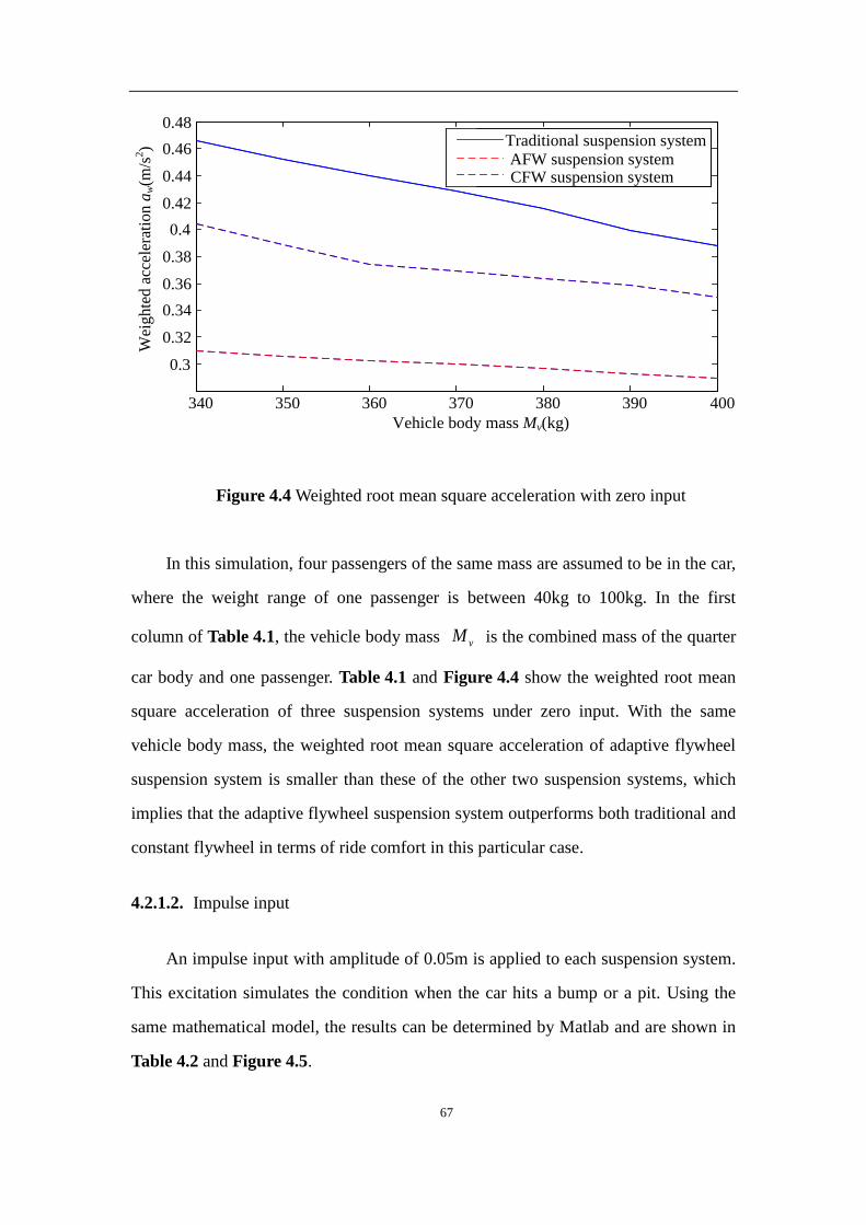
67
340 350 360 370 380 390 400
0.3
0.32
0.34
0.36
0.38
0.4
0.42
0.44
0.46
0.48
Vehicle body mass Mv(kg)
Wei
ghte
d a
ccel
erat
ion a
w(m
/s2)
Traditional suspension system
AFW suspension systemCFW suspension system
Figure 4.4 Weighted root mean square acceleration with zero input
In this simulation, four passengers of the same mass are assumed to be in the car,
where the weight range of one passenger is between 40kg to 100kg. In the first
column of Table 4.1, the vehicle body mass vM is the combined mass of the quarter
car body and one passenger. Table 4.1 and Figure 4.4 show the weighted root mean
square acceleration of three suspension systems under zero input. With the same
vehicle body mass, the weighted root mean square acceleration of adaptive flywheel
suspension system is smaller than these of the other two suspension systems, which
implies that the adaptive flywheel suspension system outperforms both traditional and
constant flywheel in terms of ride comfort in this particular case.
4.2.1.2. Impulse input
An impulse input with amplitude of 0.05m is applied to each suspension system.
This excitation simulates the condition when the car hits a bump or a pit. Using the
same mathematical model, the results can be determined by Matlab and are shown in
Table 4.2 and Figure 4.5.

68
Table 4.2 Weighted root mean square acceleration with impulse input
Vehicle
body
mass
vM (kg)
Weighted
acceleration of
traditional
suspension
system aw(m/s2)
Weighted
acceleration of
CFW suspension
system aw(m/s2)
Weighted
acceleration of
AFW suspension
system aw(m/s2)
340 0.4878 0.3858 0.2782
350 0.4684 0.3746 0.2746
360 0.4546 0.3689 0.2715
370 0.4398 0.3625 0.2679
380 0.4264 0.3589 0.2643
390 0.4112 0.3532 0.2622
400 0.3986 0.3478 0.2598
340 350 360 370 380 390 4000.25
0.3
0.35
0.4
0.45
0.5
Wei
ghte
d a
ccel
erat
ion a
w(m
/s2)
Traditional suspension system
AFW suspension systemCFW suspension system
Vehicle body mass Mv(kg)
Figure 4.5 Weighted root mean square acceleration with impulse input
Table 4.2 and Figure 4.5 show the weighted root mean square acceleration of the
three suspension systems under impulse input. The weighted root mean square
acceleration of adaptive flywheel suspension system is again the smallest of the three

69
suspension system under the same vehicle body mass. This indicates that the adaptive
flywheel suspension system performs better than the other two suspension system.
4.2.1.3. Sinusoidal input
A sinusoidal input with amplitude 0.05m and frequency 5Hz is applied to each
suspension system. The wave length of this sinusoidal input is 4m, which indicates
that the speed of the vehicle is approximately 80km/h. This excitation simulates the
car running on a rough road.
Table 4.3 Weighted root mean square acceleration with sinusoidal input
Vehicle
body
mass vM
(kg)
Weighted
acceleration of
traditional
suspension
system
Weighted
acceleration of
CFW suspension
system aw(m/s2)
Weighted
acceleration of
AFW suspension
system aw(m/s2)
340 1.9786 2.8434 3.9845
350 1.8498 2.7969 3.7459
360 1.7249 2.7425 3.5315
370 1.6256 2.6998 3.3464
380 1.5143 2.6312 3.1956
390 1.3983 2.5786 3.0978
400 1.2964 2.5146 3.0364

70
340 350 360 370 380 390 4001
1.5
2
2.5
3
3.5
4
Traditional suspension system
AFW suspension systemCFW suspension system
Wei
ghte
d a
ccel
erat
ion a
w(m
/s2)
Vehicle body mass Mv(kg)
Figure 4.6 Weighted root mean square acceleration with sinusoidal input
As shown in Table 4.3 and Figure 4.6, with sinusoidal input, the results of the
three suspension systems are opposite to those obtained when comparing the two
other inputs. Here, the weighted root mean square acceleration of the adaptive
flywheel suspension system is larger than both other suspension systems, which
implies that the adaptive flywheel suspension system gives the worst performance of
the three chosen suspension systems under the case of a sinusoidal input. With the
sinusoidal input, the adaptive flywheel will consistently generate a large inertial force.
However the gravitational mass of this vehicle is constant, which eventually leads to a
higher weighted root mean square acceleration.
4.2.2. Tire grip
Tire grip is another key factor to evaluate the performance of a suspension
system, and can be used to characterize the ride safety of a vehicle. The tire grip can
be quantified as [180,181]:
1
22 0 2 2
0.2 ( ( ) ) ( )qM G n v H s (4.17)

71
In equation (4.17), 2M is the tire grip index, where 3 2 12
1
( ) ( ) ( )( )
( )
X s X s X sH s
sX s
.
As mentioned before, once the road roughness is chosen and the velocity of the car is
fixed, the transfer function 2( )H s will be the only factor to determine the tire grip.
Based on equation (4.2), the transfer function 2 ( )tH s for a traditional
suspension system can be written as:
2 2 2
2 23 2 2 2 2 2
( 2 )( ) 1
2( )(2 )
t b bt
b bt t b b
s sH s
s s s s s s
(4.18)
From equation (4.6), the transfer function 2 ( )cH s for a constant flywheel
suspension system can be presented as:
2 2 2 2
2 23 2 2 2 2 2 2 2
( 2 )( ) 1
2( )( 2 )
t b bc
b bt t b b
s s sH s
s s s s s s s s
(4.19)
For the same reason mentioned in section 5.2.1, the transfer function for an
adaptive flywheel cannot be obtained by Laplace transform. However, the tire grip
index can also be defined as the ratio between static and dynamic loads, which can be
expressed as [151]:
2 1( )
( )
ttg
T
K X XM
M M g
(4.20)
In equation (4.20) g is the acceleration due to gravity. As shown in equation (4.20),
this performance criterion is applied under a dynamic situation; otherwise the tire grip
index will reach is maximum value, which is equal to one. With a smaller tire grip
index, the possibility of a tire losing contact with the road also becomes smaller,
which implies improved vehicle safety. By using the weighted root mean square, an
accurate tire grip index can be obtained as [182]:

72
1
22
0
1( )
T
wtg tgM M t dtT
(4.21)
By combining equation (4.21) with (4.1), (4.4) and (4.8), the numerical solution of the
weighted root mean square tire grip index for each suspension system in the
time-domain can be calculated with Matlab. The same simulation strategy is applied in
this set of simulations; namely zero, impulse and sinusoidal inputs were evaluated.
4.2.2.1. Zero input
An initial displacement 0.05m is applied to the three suspension systems. The
results can be found in Table 4.4.
Table 4.4 Weighted root mean square tire grip index with zero input
Vehicle body mass
vM (kg)
Weighted tire
grip index of
traditional
suspension
system wtgM
Weighted tire grip
index of CFW
suspension system
wtgM
Weighted tire grip
index of AFW
suspension system
wtgM
340 0.3156 0.2078 0.0684
350 0.3012 0.1996 0.0669
360 0.2874 0.1922 0.0656
370 0.2756 0.1854 0.0644
380 0.2649 0.1789 0.0631
390 0.2551 0.1731 0.0619
400 0.2462 0.1680 0.0608

73
340 350 360 370 380 390 4000.05
0.1
0.15
0.2
0.25
0.3
0.35
0.4
Wei
gh
ted
ro
ot
mea
n s
qu
are
tire
gri
p i
nd
ex M
wtg
Traditional suspension system
AFW suspension systemCFW suspension system
Vehicle body mass Mv(kg)
Figure 4.7 Weighted root mean square tire grip index with zero input
In Table 4.4 and Figure 4.7, weighted root mean square tire grip index of the
three suspension systems under zero input are shown. Compared to other two
suspension systems, the weighted root mean square tire grip index of the adaptive
flywheel suspension system is the smallest. Since the smaller weighted root mean
square tire grip index implies higher vehicle safety, the adaptive flywheel suspension
system shows better outcome than both the other suspension systems under this
condition.
4.2.2.2. Impulse input
An impulse input with amplitude of 0.05m is applied to each suspension system.
The results are shown in Table 4.5 and Figure 4.8.
Table 4.5 Weighted root mean square tire grip index with impulse input
Vehicle body mass
vM (kg)
Weighted tire
grip index of
traditional
Weighted tire grip
index of CFW
suspension system
Weighted tire grip
index of VMI
suspension system

74
suspension
system wtgM
wtgM wtgM
340 0.3879 0.2216 0.1214
350 0.3624 0.2101 0.1173
360 0.3412 0.1997 0.1131
370 0.3208 0.1894 0.1094
380 0.3001 0.1798 0.1058
390 0.2814 0.1709 0.1021
400 0.2628 0.1618 0.0986
340 350 360 370 380 390 4000.05
0.1
0.15
0.2
0.25
0.3
0.35
0.4
Vehicle body mass Mv(kg)
Traditional suspension system
AFW suspension systemCFW suspension system
Wei
ghte
d r
oot
mea
n s
quar
e ti
re g
rip i
ndex
Mw
tg
Figure 4.8 Weighted root mean square tire grip index with impulse input
Table 4.5 and Figure 4.8 show the weighted root mean square tire grip index of
three suspension systems with an impulse input. Since the weighted root mean square
tire grip index of the adaptive flywheel suspension system is still the smallest of all
three suspension systems under the same vehicle body mass, it follows that it
out-performs the constant flywheel suspension system and the traditional suspension
system.

75
4.2.2.3. Sinusoidal input
A sinusoidal input with wave length of 4m, amplitude of 0.05m and a frequency
of 5Hz is applied to each suspension system. The results are shown in Table 4.6 and
Figure 4.9,
Table 4.6 Weighted root mean square tire grip index with sinusoidal input
Vehicle body mass
vM (kg)
Weighted tire
grip index of
traditional
suspension
system wtgM
Weighted tire grip
index of CFW
suspension system
wtgM
Weighted tire grip
index of AFW
suspension system
wtgM
340 0.8458 0.6546 0.4516
350 0.8014 0.6234 0.4214
360 0.7624 0.5933 0.3907
370 0.7256 0.5646 0.3620
380 0.6929 0.5378 0.3346
390 0.6614 0.5116 0.3098
400 0.6319 0.4876 0.2844
340 350 360 370 380 390 4000.2
0.3
0.4
0.5
0.6
0.7
0.8
0.9
1
Vehicle body mass Mv(kg)
Traditional suspension system
AFW suspension systemCFW suspension system
Wei
ghte
d r
oot
mea
n s
quar
e ti
re g
rip i
ndex
Mw
tg

76
Figure 4.9 Weighted root mean square tire grip index with sinusoidal input
From Table 4.6 and Figure 4.9, under the same road conditions with the same
velocity, and for the same vehicle body mass, the adaptive flywheel suspension
system provides the smallest weighted root mean square tire grip index. Based on this,
the adaptive flywheel suspension system provides a higher safety performance than
both the traditional suspension system and the constant flywheel suspension system.
4.2.3. Vehicle body deflection
The vehicle body deflection is the last important factor for evaluating the
performance of a suspension system. This performance criterion corresponds to the
vehicle center of gravity, which will affect the working life of a suspension system,
and can be determined as [183,184]:
1
23 0 3 2
0.2 ( ( ) ) ( )qM G n v H s (4.22)
In equation (4.22), 3M is the vehicle body deflection index, and 23
1
( )( )
( )
X sH s
sX s . As
outlined above, the vehicle body deflection is completely determined by the transfer
function 3( )H s .
By rewriting equation (4.2), the transfer function 3 ( )tH s for a traditional
suspension system can be presented as:
2
3 22 2 2 2 2 2
( )2
( )(2 )
tt
b bt t b b
sH s
s s s s s
(4.23)
From equation (4.6), the new transfer function 3 ( )cH s for a constant flywheel
suspension system can be rewritten as:

77
2
3 22 2 2 2 2 2 2 2
( )2
( )( 2 )
tc
b bt t b b
sH s
s s s s s s s
(4.24)
Due to the non-linearity of the adaptive flywheel, the transfer function of the
adaptive flywheel cannot be acquired by Laplace transform. However, as mentioned
above, the vehicle body deflection is related to the vehicle center gravity, which
implies that it can be expressed as:
3 2fD X X (4.25)
By using the same weighted root mean square method, an accurate vehicle body
deflection can be calculated as [185,186]:
1
22
0
1( )
T
fw fD D t dtT
(4.26)
By combining equation (4.26) with (4.1), (4.4) and (4.8), the numerical solution of
weighted root mean square vehicle body deflection for each suspension system in the
time-domain can be calculated via Matlab. The same initial conditions and simulation
strategy are applied in this simulation as for the simulations of riding comfort and tire
grip index.
4.2.3.1. Zero input
An initial displacement 0.05m is applied on the three suspension systems. The
results are shown in Table 4.7 and Figure 4.10.
Table 4.7 Weighted root mean square vehicle body deflection with zero input
Vehicle body mass
vM (kg)
Weighted
vehicle body
deflections of
traditional
suspension
system Dfw(m)
Weighted vehicle
body deflections of
CFW suspension
system Dfw(m)
Weighted vehicle
body deflections of
AFW suspension
system Dfw(m)

78
340 0.0035 0.0035 0.0035
350 0.0035 0.0035 0.0034
360 0.0035 0.0035 0.0034
370 0.0035 0.0034 0.0034
380 0.0034 0.0034 0.0033
390 0.0034 0.0034 0.0033
400 0.0034 0.0034 0.0033
340 350 360 370 380 390 4000
0.5
1
1.5
2
2.5
3
3.5
4
4.5
5x10
-3
Wei
gh
ted
v
ehic
le b
od
y d
efle
ctio
ns
Dfw
(m
)
Traditional suspension system
AFW suspension systemCFW suspension system
Vehicle body mass Mv(kg)
Figure 4.10 Weighted root mean square vehicle body deflection with zero input
Based on Table 4.7and Figure 4.10, the three suspension systems show almost
the same weighted root mean square vehicle body deflection under zero input. This
implies that the proposed adaptive flywheel suspension system shows no
improvement compared to the other two suspension systems.
4.2.3.2. Impulse input
An impulse input with amplitude 0.05m is applied to each suspension system.
The results are shown in Table 4.8.

79
Table 4.8 Weighted root mean square vehicle body deflection with impulse input
Vehicle body mass
vM (kg)
Weighted
vehicle body
deflections of
traditional
suspension
system Dfw(m)
Weighted vehicle
body deflections of
CFW suspension
system Dfw(m)
Weighted vehicle
body deflections of
AFW suspension
system Dfw(m)
340 0.0031 0.0031 0.0030
350 0.0031 0.0031 0.0030
360 0.0031 0.0031 0.0030
370 0.0031 0.0031 0.0030
380 0.0031 0.0031 0.0030
390 0.0031 0.0031 0.0030
400 0.0031 0.0031 0.0030
340 350 360 370 380 390 4000
0.5
1
1.5
2
2.5
3
3.5
4
4.5
5x10
-3
Vehicle body mass Mv(kg)
Traditional suspension system
AFW suspension systemCFW suspension system
Wei
gh
ted
v
ehic
le b
od
y d
efle
ctio
ns
Dfw
(m
)
Figure 4.11 Weighted root mean square vehicle body deflection with impulse input

80
From Table 4.8 and Figure 4.11, similar results can be found as for the case of
zero input. The weighted root mean square vehicle body deflection of the three
suspension systems are almost identical, which indicates there is almost no
performance difference in vehicle body deflection for each suspension system.
4.2.3.3. Sinusoidal input
A sinusoidal input with wave length of 4m, amplitude 0.05m and frequency 5Hz
is applied to each suspension system. The results are shown in Table 4.9 and Figure
4.12.
Table 4.9 Weighted root mean square vehicle body deflectionwith sinusoidal
input
Vehicle body mass
vM (kg)
Weighted
vehicle body
deflections of
traditional
suspension
system Dfw(m)
Weighted vehicle
body deflections of
CFW suspension
system Dfw(m)
Weighted vehicle
body deflections of
AFW suspension
system Dfw(m)
340 0.0096 0.0096 0.0168
350 0.0095 0.0095 0.0164
360 0.0093 0.0092 0.0161
370 0.0091 0.0091 0.0157
380 0.0090 0.0090 0.0153
390 0.0088 0.00889 0.0148
400 0.0087 0.0087 0.0144

81
340 350 360 370 380 390 4000.008
0.009
0.01
0.011
0.012
0.013
0.014
0.015
0.016
0.017
Vehicle body mass Mv(kg)
Traditional suspension system
AFW suspension systemCFW suspension system
Wei
gh
ted
v
ehic
le b
od
y d
efle
ctio
ns
Dfw
(m
)
Figure 4.12 Weighted root mean square vehicle body deflection with sinusoidal input
Table 4.9 and Figure 4.12 show the weighted root mean square vehicle body
deflection of the three different suspension systems with sinusoidal input. The
weighted root mean square vehicle body deflection of the adaptive flywheel is greater
than the other two suspension systems, which implies that in this case, the traditional
suspension system and the constant flywheel suspension system show better results
than the adaptive flywheel suspension system.
4.3. Performance evaluation for different changing ratio
In the previous subsections, the three different suspension systems were
evaluated by three performance criteria. The results of simulations indicate that the
performance of a suspension system of a two-terminal device with adaptive flywheel
is better than that of the other suspension systems under most circumstances in terms
of ride comfort and tire grip. However, the suspension system of a two-terminal
device with adaptive flywheel exhibits the worst performance in terms of body
deflection. In order to further analyze the characteristics of the two-terminal device

82
with an adaptive flywheel, another important simulation is also conducted in the
research.
In this simulation, the only variable is the changing ratio of the adaptive flywheel,
all the other parameters are kept the same. As mentioned in chapter 3, by reducing the
weight of the frame, the changing ratio of the adaptive flywheel will increase.
However, with the reduced weight, the frame will be more fragile, which will lead to
low reliability. Moreover, the removal of additional material from the frame will not
only make it difficult to manufacture, but also increase material waste, and both
factors will increase cost. Therefore, in this simulation, the changing ratio is varied
from 5% to 55%.
4.3.1. First situation: zero input
Assume an initial displacement 0.05m is applied to the quarter car model, the only
variable is the changing ratio of the adaptive flywheel. The results of simulation are
shown in Table 4.10. In Table 5.10, the index value for all three indices are the values
obtained in the prior simulation results shown in Table 4.1, Table 4.4 and Table 4.7
when the vehicle body mass is 370kg.
Table 4.10 Performance with different changing ratio under zero input
Changing ratio of
moment of inertia
(%)
Weighted
acceleration of
AFW
suspension
system
aw(m/s2)
Weighted tire
grip index of
AFW
suspension
system wtgM
Weighted
vehicle body
deflection of
AFW
suspension
system Dfw(m)
Index value of
traditional
suspension system
0.4288 0.2756 0.0035

83
5 0.3598 0.1681 0.0025
10 0.3486 0.1507 0.0027
15 0.3371 0.1299 0.0027
20 0.3249 0.1083 0.0026
25 0.3111 0. 0849 0.0026
30 0.2942 0.0598 0.0025
35
40
0.2808
0.2682
0.0484
0.0417
0.0025
0.0025
45 0.2579 0.0387 0.0027
50 0.2483 0.0359 0.0026
55 0.2401 0.0341 0.0026
0 10 20 30 40 50 600.24
0.26
0.28
0.3
0.32
0.34
0.36
Changing ratio of moment of inertia (%)
Wei
ghte
d a
ccel
erat
ion a
w(m
/s2)
Figure 4.13 Weighted accelerations of AFW suspension system with different
changing ratios under zero input

84
0 10 20 30 40 50 60
0.04
0.06
0.08
0.1
0.12
0.14
0.16
Changing ratio of moment of inertia (%)Wei
gh
ted
ro
ot
mea
n s
qu
are
tire
gri
p i
nd
ex M
wtg
Figure 4.14 Weighted tire grip index of AFW suspension system with different
changing ratios under zero input
5 10 15 20 25 30 35 40 45 50 550
0.5
1
1.5
2
2.5
3
3.5
4x10
-3
Changing ratio of moment of inertia (%)
Wei
gh
ted
v
ehic
le b
od
y d
efle
ctio
ns
Dfw
(m
)
Figure 4.15 Weighted suspension deflections of AFW suspension system with
different changing ratios under zero input
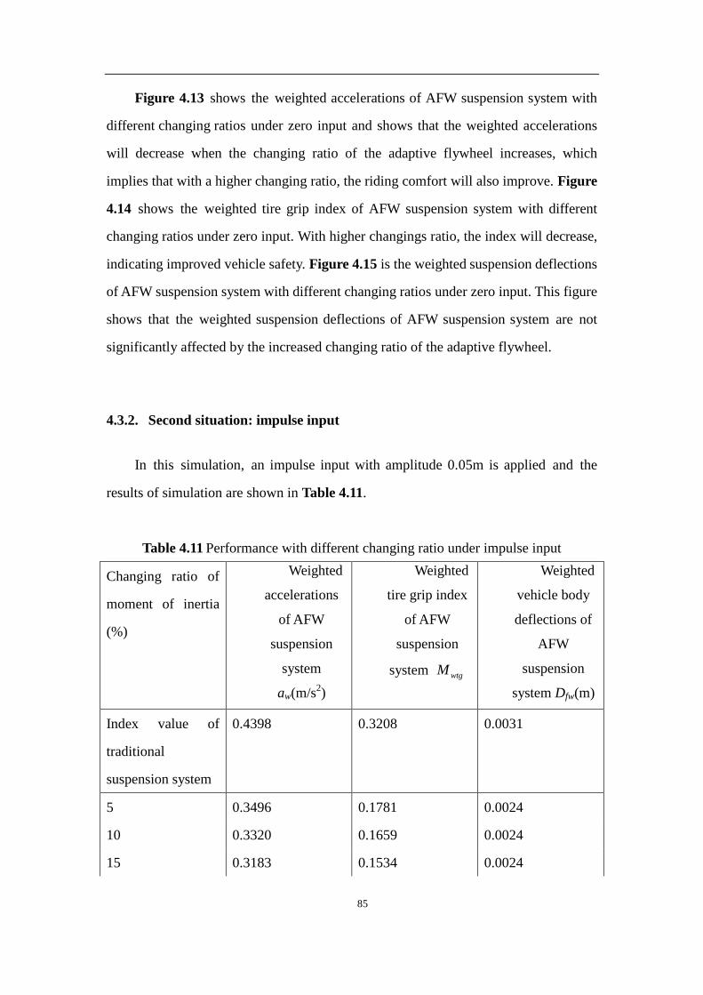
85
Figure 4.13 shows the weighted accelerations of AFW suspension system with
different changing ratios under zero input and shows that the weighted accelerations
will decrease when the changing ratio of the adaptive flywheel increases, which
implies that with a higher changing ratio, the riding comfort will also improve. Figure
4.14 shows the weighted tire grip index of AFW suspension system with different
changing ratios under zero input. With higher changings ratio, the index will decrease,
indicating improved vehicle safety. Figure 4.15 is the weighted suspension deflections
of AFW suspension system with different changing ratios under zero input. This figure
shows that the weighted suspension deflections of AFW suspension system are not
significantly affected by the increased changing ratio of the adaptive flywheel.
4.3.2. Second situation: impulse input
In this simulation, an impulse input with amplitude 0.05m is applied and the
results of simulation are shown in Table 4.11.
Table 4.11 Performance with different changing ratio under impulse input
Changing ratio of
moment of inertia
(%)
Weighted
accelerations
of AFW
suspension
system
aw(m/s2)
Weighted
tire grip index
of AFW
suspension
system wtgM
Weighted
vehicle body
deflections of
AFW
suspension
system Dfw(m)
Index value of
traditional
suspension system
0.4398 0.3208 0.0031
5 0.3496 0.1781 0.0024
10 0.3320 0.1659 0.0024
15 0.3183 0.1534 0.0024

86
20 0.2994 0.1387 0.0023
25 0.2803 0.1241 0.0024
30 0.2612 0.1059 0.0022
35
40
0.2443
0.2286
0.0913
0.0789
0.0023
0.0024
45 0.2134 0.0681 0.0023
50 0.2011 0.0595 0.0023
55 0.1897 0.0356 0.0022
0 10 20 30 40 50 60
0.2
0.22
0.24
0.26
0.28
0.3
0.32
0.34
Changing ratio of moment of inertia (%)
Wei
gh
ted
acc
eler
atio
n a
w(m
/s2)
Figure 4.16 Weighted accelerations of AFW suspension system with different
changing ratios under impulse input

87
0 10 20 30 40 50 60
0.04
0.06
0.08
0.1
0.12
0.14
0.16
Changing ratio of moment of inertia (%)Wei
ghte
d r
oot
mea
n s
quar
e ti
re g
rip i
ndex
Mw
tg
Figure 4.17 Weighted tire grip index of AFW suspension system with different
changing ratios under impulse input
5 10 15 20 25 30 35 40 45 50 550
0.5
1
1.5
2
2.5
3x10
-3
Changing ratio of moment of inertia (%)
Wei
gh
ted
v
ehic
le b
od
y d
efle
ctio
ns
Dfw
(m
)
Figure 4.18 Weighted vehicle body deflections of AFW suspension system with
different changing ratios under impulse input

88
Figure 4.16 shows the relationship between the weighted accelerations of the
AFW suspension system and different changing ratios of the adaptive flywheel under
impulse input. With an increase in the changing ratio of the adaptive flywheel, the
weighted acceleration will decrease. This result again indicates that higher changing
ratio of adaptive flywheel will improve the riding comfort. Figure 4.17 is the
weighted tire grip index of AFW suspension system with different changing ratio under
impulse input. This shows that the weighted tire grip index will decrease with
increasing the changing ratio, which implies the vehicle safety improves under
increasing changing ratio. Figure 4.18 is the weighted suspension deflections of AFW
suspension system with different changing ratio under impulse input. With the
variable changing ratio, the weighted suspension deflections of AFW suspension
system almost stay the same. Therefore, the changing ratio of the adaptive flywheel
does not affect the weighted suspension deflections of the AFW suspension system.
4.3.3. Third situation: sinusoidal excitation
In the final simulation, a sinusoidal input with amplitude 0.05m and frequency
5Hz is applied as excitation. Results about this simulation can be found in Table 4.12.
Table 4.12 Performance with different changing ratio under sinusoidal input
Changing ratio of
moment of inertia
(%)
Weighted
accelerations
of AFW
suspension
system
aw(m/s2)
Weighted
tire grip index
of AFW
suspension
system wtgM
Weighted
vehicle body
deflections of
AFW
suspension
system Dfw(m)
Index value of
traditional
suspension system
1.6256 0.7256 0.0091
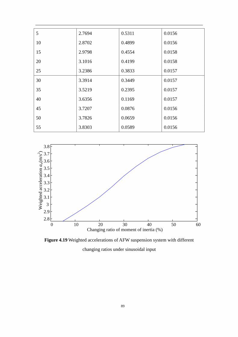
89
5 2.7694 0.5311 0.0156
10 2.8702 0.4899 0.0156
15 2.9798 0.4554 0.0158
20 3.1016 0.4199 0.0158
25 3.2386 0.3833 0.0157
30 3.3914 0.3449 0.0157
35
40
3.5219
3.6356
0.2395
0.1169
0.0157
0.0157
45 3.7207 0.0876 0.0156
50 3.7826 0.0659 0.0156
55 3.8303 0.0589 0.0156
0 10 20 30 40 50 60
2.8
2.9
3
3.1
3.2
3.3
3.4
3.5
3.6
3.7
3.8
Changing ratio of moment of inertia (%)
Wei
gh
ted
acc
eler
atio
n a
w(m
/s2)
Figure 4.19 Weighted accelerations of AFW suspension system with different
changing ratios under sinusoidal input

90
0 10 20 30 40 50 60
0.1
0.15
0.2
0.25
0.3
0.35
0.4
0.45
0.5
Changing ratio of moment of inertia (%)
Wei
gh
ted
ro
ot
mea
n s
qu
are
tire
gri
p i
nd
ex M
wtg
Figure 4.20 Weighted tire grip index of AFW suspension system with different
changing ratios under sinusoidal input
5 10 15 20 25 30 35 40 45 50 550
0.002
0.004
0.006
0.008
0.01
0.012
0.014
0.016
0.018
0.02
Changing ratio of moment of inertia (%)
Wei
gh
ted
v
ehic
le b
od
y d
efle
ctio
ns
Dfw
(m
)
Figure 4.21 Weighted vehicle body deflections of AFW suspension system with
different changing ratios under sinusoidal input

91
Figure 4.19 is the weighted accelerations of the AFW suspension system with
different changing ratios. However, the results of simulation are different from both
prior simulation results and show that with increased changing ratio of the adaptive
flywheel, the weighted accelerations of AFW suspension system also increase, which
implies that the riding comfort worsens. Figure 4.20 is the weighted tire grip index of
AFW suspension system with different changing ratios under sinusoidal input. The
results of this simulation indicate that the weighted tire grip index of AFW suspension
system will decrease when the changing ratio increases. Figure 4.21 shows the
weighted suspension deflections of AFW suspension system with different changing
ratios. The results in this case are the same as the former simulation; the variable
changing ratio does not affect the weighted suspension deflections of AFW suspension
system.
4.3.4. Optimal changing ratio for adaptive flywheel
4.3.4.1. Determination of optimal changing ratio for adaptive flywheel
As mentioned above, with different inputs and different changing ratios of the
adaptive flywheel, the performance of the AFW suspension system is quite different.
In the previous simulations, three different road conditions (zero input, impulse input
and sinusoidal input) and three different suspension performance criteria are
introduced, and the evaluations are carried out to show the improvement of the
proposed situation. However, the results show that the proposed suspension system
does not always show better performance than other two suspension systems.
Therefore, under the right conditions, an optimal changing ratio of adaptive flywheel
for suspension system can be determined. To calculate the optimal changing ratio,
three other factors need to be considered.
The first one is the proportion of road situation. At the beginning of this chapter,
zero input, impulse input and sinusoidal input are introduced as three different road

92
conditions. However, these three road conditions always appear with different
proportion in a real case, the actual proportion of each road condition is critical for the
calculation of optimal changing ratio [178,179].
The second factor is the proportion of performance criteria. In our simulations,
riding comfort, tire grip and suspension deflection are applied to evaluate the
suspension system. For the proposed suspension system, the results are conflicting
under these three performance criteria. In order to find an optimal result, the
important index for different performance criteria need to be classified, which will be
expressed as the proportion [155,180].
The final one is the cost of manufacture of the adaptive flywheel. With the higher
changing ratio, there will be more waste of materials (the cut out materials such as
slots and holes). When the changing ratio reaches a certain level, the manufacture
time will increase, due to the small size of this flywheel. All the reasons will cause an
increase in cost [187,188]. The detailed discussions of these three factors will be
introduced in a later sub-section.
According to Figure 4.15, Figure 4.18 and Figure 4.21, the weighted suspension
deflections of the AFW suspension system are independent of the variable changing
ratio of the adaptive flywheel. This implies that this performance criterion can be
excluded from the determination of the optimal changing ratio for the adaptive
flywheel.
Assume that the relationship between the weighted accelerations of AFW
suspension system and changing ratio under zero input can be presented as:
( )zw zaf x (4.27)
where zw is the weighted acceleration under zero input, x is the changing ratio. Also
assume that the relationship between the weighted tire grip index of the AFW
suspension system and changing ratio under zero input can also be described as:
( )ztgw ztgM f x (4.28)

93
where ztgwM is the weighted tire grip index with zero input.
The same assumptions can be made for impulse input and sinusoidal input:
( )
( )
( )
( )
iw ia
itgw itg
sw sa
stgw stg
f x
M f x
f x
M f x
(4.29)
where iw is the weighted accelerations under impulse input, itgwM is the weighted
tire grip index with impulse input, sw is the weighted accelerations with sinusoidal
input and stgwM is the weighted tire grip index with sinusoidal input. Since there are
two performance criteria, the proportion of performance between the two factors
needs to be considered. New performance criteria can be written as:
Zero input: 1 2
1 2
( )
1
ztgwzwzp
szw sztgw
Mf x x x
M
x x
(4.30)
Here, ( )zpf x is the performance function with zero input, szw is the weighted
accelerations of the traditional suspension system with zero input, sztgwM is the
weighted tire grip index with zero input, and 1x is the performance proportion of
riding comfort while 2x is performance proportion of tire grip. Similarly, for an
impulse input, a performance function can be defined as
Impulse input:1 2
1 2
( )
1
itgwiwip
siw sitgw
Mf x x x
M
x x
(4.31)
Here, ( )ipf x is the performance function with impulse input, siw represents the
weighted accelerations of the traditional suspension system with impulse input, and
sitgwM is the weighted tire grip index with impulse input. Finally, for a sinusoidal
input
94
Sinusoidal input:1 2
1 2
( )
1
stgwswsp
ssw sstgw
Mf x x x
M
x x
(4.32)
Here, ( )spf x is performance function with sinusoidal input, ssw represents the
weighted accelerations of the traditional suspension system with sinusoidal input, and
sstgwM is weighted tire grip index with sinusoidal input.
In these simulations, zero input, impulse input and sinusoidal input are used for
simulating the different road situations. However, in most cases, an actual road
situation is divided into these three situations with different proportions. By
combining equations (4.30), (4.31) and (4.32), a new performance equation can be
determined as
3 4 5
3 4 5
( ) ( ) ( ) ( )
1
p zp ip spf x f x x f x x f x x
x x x
(4.33)
where ( )pf x is the overall performance function, 3x is the proportion of zero input, 4x
is the proportion of impulse input and 5x represents the proportion of sinusoidal
input.
Based on equation (4.33), when the value of ( )pf x is minimum, the suspension
system indicates best performance. Therefore, the determination of optimal changing
ratio depends on the determination of the minimum value of ( )pf x . Additionally,
another important factor also needs to be evaluated. As mentioned at the beginning of
this sub-section, with an increase in changing ratio, the cost of the adaptive flywheel
will rise. In the simulations, the cost of manufacturing adaptive flywheel is divided
into two parts, waste of materials and working hours. According to China labor wage
reports and Chongqing average labor cost, when the changing ratio is under 20%, the
relationship between cost and changing ratio is linear. The function of cost can be
written as [187,188]:
95
2
( ) 1 0.8 ( 0.2)
( ) 1.16 ( 0.8) ( 0.2)
c
c
f x x x
f x x x
(4.34)
From equation (4.33) and (4.34), the determination of the optimal changing ratio can
be done minimizing two objective functions ( )pf x and ( )cf x , i.e.,
min ( ) min ( )p cf x f x (4.35)
subject to constraints (4.30) to (4.34).
4.3.4.2. Determination of optimal changing ratio by Chebyshev goal
programming
Based on equation (4.15), the determination of optimal changing ratio can be
considered as a multi-objective optimization problem. In this thesis, due to its
simplicity in modelling and computation processes, Chebyshev goal programming is
applied to determine the optimal changing ratio.
For single objective performance under zero input, changing ratio zabx and ztgbx
represents the best performance for weighted accelerations zabf and weighted tire
grip ztgbf . Similarly, the worst performance of weighted accelerations zawf and
weighted tire grip ztgwf correspond to changing ratio zawx and ztgwx . Under impulse
input, the best performance of weighted accelerations iabf and weighted tire grip
itgbf is due to the changing ratio iabx and itgbx , and the worst performance of
weighted accelerations iawf and weighted tire grip itgwf is due to the changing ratio
iawx and itgwx . For sinusoidal input, best performance of weighted accelerations sabf
and weighted tire grip stgbf is due to changing ratio sabx and stgbx , and the worst
performance of weighted accelerations sawf and weighted tire grip stgwf is due to
changing ratio sawx and stgwx . Assume there is a multi-objective optimal changing

96
ratio optx which is related to the best performance aoptf and tgoptf . By using
Chebyshev goal programming, the new equation can be written as:
min r (4.36)
subject to
aopt zab
r
zaw zab
aopt iab
r
iaw iab
aopt sab
r
saw sab
tgopt ztgb
r
ztgw ztgb
tgopt itgb
r
itgw itgb
tgopt stgb
r
stgw stgb
f f
f f
f f
f f
f f
f f
f f
f f
f f
f f
f f
f f
(4.37)
Through equation (4.36) and (4.37), the optimal changing ratio for the adaptive
flywheel can be found. This optimal changing ratio is based on three assumptions.
First, the riding comfort is as important as tire grip. The other assumption is that the
proportion of inputs are identical, which implies that the road surface is equally
distributed between three situations. Finally, the cost of this flywheel is excluded for
this optimal changing ratio. However, for a real case, tire grip is more important than
riding comfort, and the road situation is quite different.
In order to calculate the optimal changing ratio for the adaptive flywheel
suspension system, the performance proportion and the proportion of inputs need to
be determined. According Rath and Zhao [155,180], the performance proportion of
riding comfort 1x and safety 2x can be taken to be 0.35 and 0.65, respectively. Based
on research conducted by Wang, the proportion of zero input 3x , impulse input 4x
and sinusoidal input 5x is chosen as 0.1, 0.5 and 0.4 respectively [178]. By

97
considering all these factors and equation (4.30) to (4.33), a new Chebyshev goal
programming model can be formulated as:
min , (4.38)
subject to
optp pb
pw pb
optc cb
cw cb
f f
f f
f f
f f
(4.39)
and all other constraints are the same as for the single objective performance. In
equation (4.39), optpf is the multi-objective optimal best performance, pbf is the
single-objective best performance, pwf represents the single-objective worst
performance, optcf is the multi-objective optimal cost, cbf is the single-objective
best cost, and cwf is the single-objective worst cost.
By substituting equation (4.38) and (4.39) with the results of Table 4.10, Table
4.11 and Table 4.12, the optimal changing ratio of adaptive flywheel for suspension
system can be determined as 0.258x . This implies that under this changing ratio,
the suspension system with the adaptive flywheel shows the best performance at the
lowest cost. This optimal changing ratio of adaptive flywheel for suspension system is
obtained under the specific choices of 1x to 5x selected above, which are a function
of cost, performance proportion and the proportion of inputs. Any change of these
conditions, the optimal changing ratio will then also be different. By this optimal
changing ratio, the performance of this suspension system with different input can be
found in Table 4.13.

98
Table 4.13 performance of AFW suspension system with different inputs under
optimal changing ratio
Input Weighted
accelerations of
AFW suspension
system aw(m/s2)
Weighted tire grip
index of AFW
suspension system
wtgM
Weighted vehicle
body deflections of
AFW suspension
system Dfw(m)
Zero input 0.3079 0.0797 0.0026
Impulse input 0.2764 0.1203 0.0024
Sinusoidal input 3.2698 0.3757 0.0157
Table 4.13 shows the performance of the AFW suspension system with different
inputs under the optimal changing ratio. Compared to the traditional suspension
system:
1) Under zero input, the weighted accelerations of AFW suspension system
decreases 28.2%, the weighted tire grip index of AFW suspension system
decreases 71.1% and the weighted vehicle body deflections of AFW
suspension system decreases 25.7%.
2) Under impulse input, the weighted accelerations of AFW suspension
system decrease 37.1%, the weighted tire grip index of AFW suspension
system weighted decreases 62.5% and the vehicle body deflections of
AFW suspension system decreases 22.6%.
3) Under sinusoidal input, the weighted accelerations of AFW suspension
system increase 101.1% (this implies that under sinusoidal input,
passengers will feel more vertical acceleration than the traditional
suspension system), the weighted tire grip index of AFW suspension
system decreases 48.2% and the weighted vehicle body deflections of
AFW suspension system increase 42%.

99
4.3.4.3. Optimal changing ratio for adaptive flywheel with different performance and
inputs proportion
As mentioned above, with a change in the function of cost, performance
proportion or proportion of inputs, the optimal changing ratio will also change.
However, there are many factors which can affect the function of cost, such as
different geographical areas, different factories and different workers, and it is
impossible to determine one universal function of cost. Moreover, many of these
factors are human factors, such as the efficiency difference between experienced and
inexperienced workers, which makes some of the costs unpredictable. Therefore, in
our simulations, the function of cost is always chosen as equation (4.34).
By fixing the proportion of inputs, the relationship between optimal changing
ratio and performance proportion can be investigated as shown in Table 4.14:
Table 4.14 Optimal changing ratio with different performance proportion
Riding comfort 1x 0.2 0.4 0.5 0.6 0.8
Safety 2x 0.8 0.6 0.5 0.4 0.2
Optimal changing
ratio x
0.378 0.301 0.231 0.211 0.198
Table 4.14 is the relationship between the optimal changing ratio and the
performance proportion and shows that with an increasing proportion of riding
comfort (or equivalently a decreasing proportion of safety), the optimal changing ratio
will decrease.
The same simulations are conducted with different conditions. By fixing the
performance proportion, the relationship between optimal changing ratio and
proportion of inputs can also be determined by equation (4.38) and (4.39). In the
proportion of inputs, there are three different types of inputs, which are zero input,

100
impulse input and sinusoidal input, respectively. Each of these types of inputs
represents a different road situation. However, in actual road situation, the proportion
of zero input is quite small (meaning under 10% in most circumstances) [178,179].
Therefore, in our simulations, the proportion of zero input is fixed at 0.1, and the
variables varied are the proportion of impulse input and sinusoidal input. The
relationship between optimal changing ratio and proportion of inputs is shown in
Table 4.15.
Table 4.15 Relationship between optimal changing ratio and proportion of inputs
Proportion of
impulse input 4x
0.1 0.3 0.45 0.6 0.8
Proportion of
sinusoidal input 5x
0.8 0.6 0.45 0.3 0.1
Optimal changing
ratio x
0.201 0.219 0.241 0.297 0.389
Table 4.15 is the relationship between optimal changing ratio and proportion of
inputs, and shows that a high proportion of impulse input (or equivalently low
proportion of sinusoidal input), the optimal changing ratio will increase.
4.4. Conclusion
In this chapter, three different suspension systems were evaluated using three of
the most commonly used performance criteria. Under zero input (initial displacement),
the AFW suspension system outperforms both traditional and constant flywheel
suspension system on riding comfort and tire grip, but shows no improvement on
vehicle body deflection. When the excitation is an impulse input, the same results as
for zero input are obtained. However, under sinusoidal input, the AFW suspension
system shows the worst results on riding comfort and vehicle body deflection. For tire

101
grip, the AFW suspension system still provides best performance.
With different changing ratio of adaptive flywheel, the performance of the AFW
suspension system is variable. When the excitation is zero input, both riding comfort
and tire grip are better with increasing changing ratio of the adaptive flywheel, but the
weighted vehicle body deflections are not affected. Under impulse input, the same
results can be found as zero input. With sinusoidal input, riding comfort decreases
when the changing ratio of adaptive flywheel increases, but the tire grip becomes
better. Vehicle body deflections are still not affected by the variable changing ratio of
the adaptive flywheel.
This optimal changing ratio of adaptive flywheel for suspension system was
obtained under specific conditions, which are a function of cost, performance
proportion and the proportion of inputs. Any change of these conditions, then the
optimal changing ratio will also be different. By increasing the proportion of riding
comfort (or equivalently decreasing the proportion of safety), the optimal changing
ratio will decrease. With a high proportion of impulse input (or equivalently low
proportion of sinusoidal input), the optimal changing ratio will increase.

102
5. Experimental identification
In the previous chapter, an ideal two-terminal system was introduced for a new
suspension system. To verify the performance of this new suspension system, actual
two-terminal device parameters are needed. To identify the key parameters of
two-terminal systems, experiments are required. In this chapter, experiments are
carried out to identify key parameters for both the two-terminal hydraulic system and
inverse screw system. After the determination of key parameters, additional
experiments are applied to verify the accuracy of these parameters and the
mathematical models of the systems. In order to minimize the spike forces during the
experiments, which are caused by the backlash, a new experiment strategy is proposed.
By adding a hydraulic rectifier, the spike forces in the two-terminal hydraulic system
are reduced, which eventually leads to higher accuracy of the mathematical model.
5.1. Experimental identification for two-terminal hydraulic
system
5.1.1. Experimental setup for two-terminal hydraulic system.
As mentioned in Section 3.2, to observe the behavior of the adaptive metal
flywheel, a two-terminal hydraulic system is applied. From equation (3.12), it is clear
that the system behavior is affected by four parameters, bah, Ffh, kh and mem, which
implies that the identification of these four key parameters is the critical next step for
analyzing the system. However, due to the complicated structure of this system,
parameters bah, Ffh, and kh cannot be calculated or measured directly, therefore
experimental identification is required.
The experimental setup of the two-terminal hydraulic device with an adaptive
flywheel is shown in Figure 5.1. An MTS 810 material test system is used for these
tests. This system can generate sinusoidal, triangular and square input signals, with
different amplitudes and frequencies. To accurately measure the rotational speed of the

103
hydraulic motor, an encoder is added to the test rig. The sampling rate for the encoder
output is set at 300Hz, the resolution of the encoder is 360/1024 degree, and the
theoretical transmission ratio of the prototype is 41rads/mm. A National Instruments
(NI) data acquisition board (NI USB-6212) is used to collect the rotational speed of the
flywheel. The parameters of the NI data acquisition board are shown in Table 5.1
1
3
2
4
5
Figure 5.1 Test rig for the adaptive flywheel (Note: 1-force cell, 2- two-terminal
hydraulic system, 3–computer, 4-actuator, 5-controller)
Table 5.1 Parameters of NI USB-6212
No. Name Specification
1 Connector Screw/68-pin SCSI
2 Analog Iputs 16
3
4
5
6
Resolution(bits)
Max Rate(kS/s)
Analog Outputs
Resolution(bites)
16
400
2
16
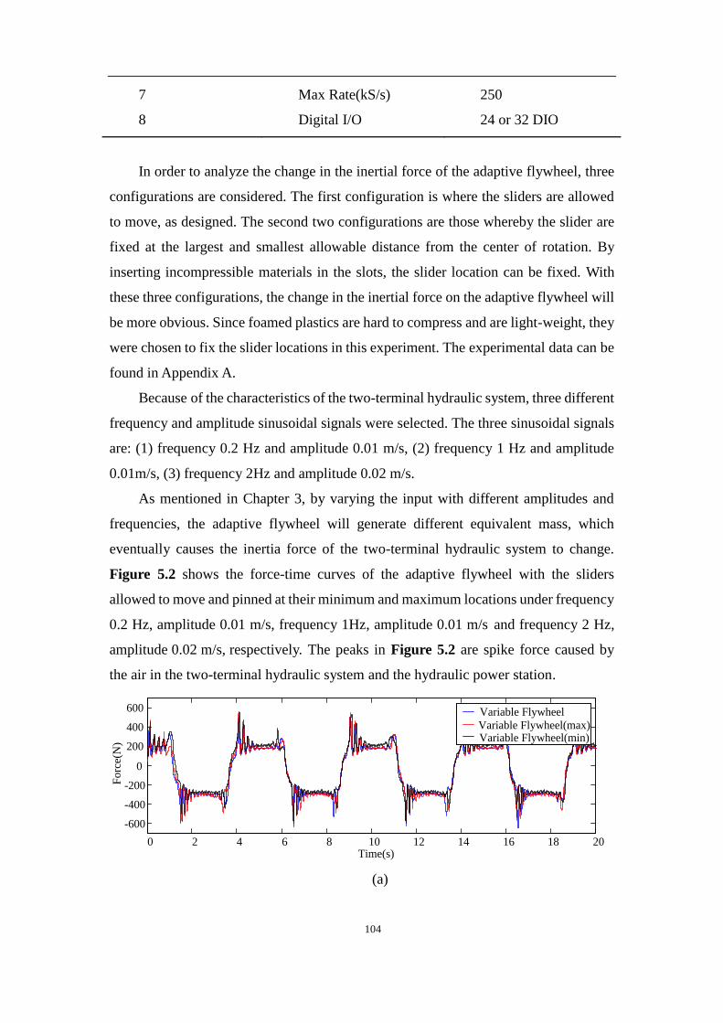
104
7
8
Max Rate(kS/s)
Digital I/O
250
24 or 32 DIO
In order to analyze the change in the inertial force of the adaptive flywheel, three
configurations are considered. The first configuration is where the sliders are allowed
to move, as designed. The second two configurations are those whereby the slider are
fixed at the largest and smallest allowable distance from the center of rotation. By
inserting incompressible materials in the slots, the slider location can be fixed. With
these three configurations, the change in the inertial force on the adaptive flywheel will
be more obvious. Since foamed plastics are hard to compress and are light-weight, they
were chosen to fix the slider locations in this experiment. The experimental data can be
found in Appendix A.
Because of the characteristics of the two-terminal hydraulic system, three different
frequency and amplitude sinusoidal signals were selected. The three sinusoidal signals
are: (1) frequency 0.2 Hz and amplitude 0.01 m/s, (2) frequency 1 Hz and amplitude
0.01m/s, (3) frequency 2Hz and amplitude 0.02 m/s.
As mentioned in Chapter 3, by varying the input with different amplitudes and
frequencies, the adaptive flywheel will generate different equivalent mass, which
eventually causes the inertia force of the two-terminal hydraulic system to change.
Figure 5.2 shows the force-time curves of the adaptive flywheel with the sliders
allowed to move and pinned at their minimum and maximum locations under frequency
0.2 Hz, amplitude 0.01 m/s, frequency 1Hz, amplitude 0.01 m/s and frequency 2 Hz,
amplitude 0.02 m/s, respectively. The peaks in Figure 5.2 are spike force caused by
the air in the two-terminal hydraulic system and the hydraulic power station.
0 2 4 6 8 10 12 14 16 18 20
-600
-400
-200
0
200
400
600
Time(s)
Fo
rce(
N)
Variable Flywheel
Variable Flywheel(max)Variable Flywheel(min)
(a)

105
0 0.5 1 1.5 2 2.5 3 3.5 4 4.5-1500
-1000
-500
0
500
1000
Time(s)
Forc
e(N
)
Variable Flywheel
Variable Flywheel(max)Variable Flywheel(min)
(b)
0 0.5 1 1.5 2 2.5 3 3.5 4 4.5-2000
-1000
0
1000
2000
Time(s)
Fo
rce(
N)
Variable Flywheel
Variable Flywheel(max)Variable Flywheel(min)
(c)
Figure 5.2 Comparison of adaptive flywheel under different configurations. (a),
(b) and (c) are force–time diagrams of three adaptive flywheels under frequency 0.2
Hz, amplitude 0.01 m/s, frequency 1Hz, amplitude 0.01 m/s and frequency 2 Hz,
amplitude 0.02 m/s respectively
It is expected that different equivalent masses would be generated by the
adaptive flywheel with the three different configurations. In Figure 5.2 (a), since the
input sinusoidal signal with low amplitude frequency can only generate a small
acceleration, this in turn leads to the changing ratio of the inertial force on the adaptive
flywheel to be less than 3%. Therefore, in Figure 5.2 (a), the three curves are almost
identical, and it is difficult to distinguish the changes in the inertial force under the
three different configurations.
However, as shown in Figure 5.2 (c), the input sinusoidal signal generates a large
acceleration because of high amplitude and frequency, which will cause a changing
ratio of inertial force on the adaptive flywheel to be as large as 11%. However, because
of the characteristics of the hydraulic system, the larger acceleration also generates
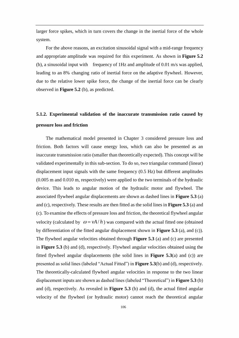
106
larger force spikes, which in turn covers the change in the inertial force of the whole
system.
For the above reasons, an excitation sinusoidal signal with a mid-range frequency
and appropriate amplitude was required for this experiment. As shown in Figure 5.2
(b), a sinusoidal input with frequency of 1Hz and amplitude of 0.01 m/s was applied,
leading to an 8% changing ratio of inertial force on the adaptive flywheel. However,
due to the relative lower spike force, the change of the inertial force can be clearly
observed in Figure 5.2 (b), as predicted.
5.1.2. Experimental validation of the inaccurate transmission ratio caused by
pressure loss and friction
The mathematical model presented in Chapter 3 considered pressure loss and
friction. Both factors will cause energy loss, which can also be presented as an
inaccurate transmission ratio (smaller than theoretically expected). This concept will be
validated experimentally in this sub-section. To do so, two triangular command (linear)
displacement input signals with the same frequency (0.5 Hz) but different amplitudes
(0.005 m and 0.010 m, respectively) were applied to the two terminals of the hydraulic
device. This leads to angular motion of the hydraulic motor and flywheel. The
associated flywheel angular displacements are shown as dashed lines in Figure 5.3 (a)
and (c), respectively. These results are then fitted as the solid lines in Figure 5.3 (a) and
(c). To examine the effects of pressure loss and friction, the theoretical flywheel angular
velocity (calculated by /vA h ) was compared with the actual fitted one (obtained
by differentiation of the fitted angular displacement shown in Figure 5.3 (a), and (c)).
The flywheel angular velocities obtained through Figure 5.3 (a) and (c) are presented
in Figure 5.3 (b) and (d), respectively. Flywheel angular velocities obtained using the
fitted flywheel angular displacements (the solid lines in Figure 5.3(a) and (c)) are
presented as solid lines (labeled “Actual Fitted”) in Figure 5.3(b) and (d), respectively.
The theoretically-calculated flywheel angular velocities in response to the two linear
displacement inputs are shown as dashed lines (labeled “Theoretical”) in Figure 5.3 (b)
and (d), respectively. As revealed in Figure 5.3 (b) and (d), the actual fitted angular
velocity of the flywheel (or hydraulic motor) cannot reach the theoretical angular

107
velocity. This verifies the existence of the pressure loss and inner friction in the
two-terminal hydraulic system.
0 2 4 6 8
-100
-50
0
50
100
Time (s)
Angula
r D
ispla
cem
ent(
deg
ree)
Actual
Fitted
0 2 4 6 8
-200
-100
0
100
200
Time (s)
Anglu
ar V
eloci
ty (
deg
ree/
s)
Actual Fitted
Theoretical
(a) (b)
0 2 4 6 8 10
-200
-100
0
100
200
Time (s)
Angula
r D
ispla
cem
ent(
deg
ree)
Actual
Fitted
0 2 4 6 8 10
-500
0
500
Time (s)
Anglu
ar V
eloci
ty (
deg
ree/
s)
Actual Fitted
Theoretical
(c) (d)
Figure 5.3 The relationship between actual fitted and theoretical flywheel
angular velocities: (a) and (c) compare the actual and fitted flywheel angular
displacements in response to the triangular command (linear) displacement inputs
(amplitudes = 0.005 m and 0.01 m respectively) applied to the two terminals of the
hydraulic device, (b) and (d) compare the actual fitted and theoretical flywheel
angular velocities obtained from (a) and (c), respectively.
5.1.3. Parameter identification
As indicated earlier, to examine the system performance, the four model
parameters in equation (3.15), ( emm , hk , ahb and fhF ) must be obtained first. Of these
four parameters, only the equivalent mass emm can be calculated, the rest have to be
identified by experiment. The theory of multi-variable solutions can be applied to this
problem. However, because of the characteristics of the mathematical model of this

108
system, some of the parameters can be eliminated by different types of experimental
inputs. The details are described in the following subsection.
5.1.3.1. Identification of damping ratio ahb and friction force fhF .
To simplify the identification process, a square command linear velocity input is
applied to the two terminals of the hydraulic device. Since the associated velocity is a
constant, i.e., v(t) = q, the acceleration is thus zero except at the direction change points.
Therefore, the third equation of equation (3.14) reduces to
( )fh ah ahF F b v t b q (5.1)
Since kh is not present in equation (5.1), kh will be identified separately whereas
parameters ahb and fhF can be determined based on the following criterion:
21
{ , } arg min ( ) ( )eh
sh
t
fh ah mh ch
t teh sh
F b F t F tt t
(5.2)
In equation (5.2), ( )mhF t is the measured force and ( )chF t is the
theoretically-calculated force using equation (5.2), sht stands for the starting time of
data recording, and eht is the end time. As the data are discrete, the above criterion can
be expressed as
2
1
1{ , } arg min ( ) ( )
1
ehn
fh ah mh ch
neh
F b F n F nn
(5.3)
where ( )mhF n is the measured force, ( )chF n is the theoretically calculated force using
equation (5.3) at sampling point n, and neh is the last sampling point of a dataset. In the
experiments, 10 datasets of rectangular velocity inputs with frequency range from 0.1
Hz to 1Hz and amplitude from 0.001m/s to 0.015m/s were collected. By using Matlab
to generate an iterative algorithm, different values of ahb and fhF can be given to
calculate the force, and the minimum difference between the calculated force and actual
force can be found. Therefore, parameters ahb and fhF are estimated as
8100 100ahb Ns/m, 190 8fhF N (5.4)
Since the values of parameters ahb and fhF are estimated, the confidence interval has

109
been included. When the difference between the calculated force and actual force is less
than 5%, the value of parameters will be recorded, which eventually leads to the range
of confidence interval.
Three typical datasets associated with frequency-amplitude combinations of
(0.2Hz and 0.002m/s), (0.5Hz and 0.0075m/s) and (1 Hz and 0.015m/s) are shown in
Figure 5.4.
0 2 4 6 8 10 12 14 16 18-5
0
5x 10
-3
Time (s)
Vel
oci
ty (
m/s
)
0 5 10 15
-1000
-500
0
500
1000
Fo
rce
(N)
Time (s)
(a) (b)
0 2 4 6 8-0.01
-0.005
0
0.005
0.01
Time (s)
Vel
oci
ty (
m/s
)
0 2 4 6 8
-1500
-1000
-500
0
500
1000
1500
Fo
rce
(N)
Time (s)
(c) (d)
0 0.5 1 1.5 2 2.5 3 3.5 4-0.02
-0.01
0
0.01
0.02
Time (s)
Vel
oci
ty (
m/s
)
0 1 2 3 4
-3000
-2000
-1000
0
1000
2000
3000
Forc
e (N
)
Time (s)
(e) (f)
Figure 5.4 Rectangular velocity inputs and corresponding measured forces. (a),
(c) and (e) present the velocity inputs with different frequencies and amplitudes
((0.2Hz 0.005m/s), (0.5Hz, 0.0075m/s) and (1Hz, 0.015m/s)) respectively. (b), (d) and
(f) are the measured forces corresponding to the velocity inputs shown in (a), (c) and

110
(e), respectively.
With the ahb and fhF values obtained above, the measured and calculated forces
based on another two sets of experimental data with frequency-amplitude combinations
(0.5Hz, 0.005m/s) and (1Hz, 0.01m/s) are compared in Figure 5.5. The velocity inputs
are shown in Figure 5.5 (a) and (c), respectively. The measured forces and calculated
forces based on the estimated ahb and fhF are presented in Figure 5.5 (b) and (d).
The close agreement between the measured and calculated forces (except at the points
where the velocity change directions) validates the accuracy of the estimated ab and
fhF .
0 2 4 6 8-0.01
-0.005
0
0.005
0.01
Time (s)
Vel
oci
ty (
m/s
)
0 1 2 3 4 5 6 7 8
-500
0
500
Time (s)
Fo
rce
(N)
Actual
Calculated
(a) (b)
0 1 2 3 4
-0.015
-0.01
-0.005
0
0.005
0.01
0.015
Time (s)
Vel
oci
ty (
m/s
)
0 1 2 3 4
-1000
-500
0
500
1000
Time (s)
Fo
rce
(N)
Actual
Calculated
(c) (d)
Figure 5.5 Comparison of the measured forces and calculated forces based on
the estimated ahb and fhF . (a) Velocity input (frequency = 0.5 Hz, amplitude =
0.005 m/s), (b) measured and calculated forces corresponding to the velocity input in
(a), (c) velocity input (frequency = 1 Hz, amplitude = 0.01 m/s), and (d) measured and
calculated forces corresponding to the velocity input in (c).

111
5.1.3.2. The variable behavior of flywheel moment of inertia Iafm and equivalent mass
emm .
As mentioned in Section 3, the equivalent mass emm will change with the input
velocity. However, when the rotational speed is very low, the slider will stay at the
initial location, emm will be minimum, and when the rotational speed reaches a
certain level, the spring in the slot will be fully compressed and emm will reach its
maximum value. To examine the general behavior of the flywheel, the input signal
should be selected in such a way that the sliders will not stay at the two ends of the slot
and hence emm will be neither the minimum nor maximum value. For this reason, a
sinusoidal input signal is chosen because it is less abrupt than the rectangular and
triangular inputs and hence the sliders can travel between the two ends but not stay at a
fixed location (i.e., one of the two ends of the slots) if the input frequency and
amplitude are properly selected. In the tests, a sinusoidal velocity input with frequency
0.1Hz and amplitude 0.0314 m/s was applied to the terminals of the hydraulic device.
Under the sinusoidal input of this frequency and amplitude, the sliders will not stay at
the initial location and the springs will not be fully compressed either, but will travel
over most of the travel range in the slots. Hence, the change of equivalent mass can be
observed over a broader range.
The variable location of the sliders, the variable moment of inertia and the
equivalent mass of the flywheel in response to the sinusoidal input (Figure 5.6(a)) can
then be calculated using equations (3.6), (3.9) and (3.12) respectively. The results are
presented in Figure 5.6 (b), (c) and (d), respectively. Figure 5.6 (c) and (d) show that
the moment of inertia and equivalent mass of the flywheel vary adaptively in response
to the input, however the variation frequency is doubled.

112
0 5 10 15 20
-0.04
-0.02
0
0.02
0.04
Time (s)
Vel
oci
ty (
m/s
)
0 5 10 15 20
0.022
0.024
0.026
0.028
0.03
0.032
0.034
0.036
Time (s)
Dis
tan
ce (
m)
(a) (b)
0 5 10 15 200.94
0.96
0.98
1
1.02
1.04
1.06x 10
-3
Time (s)
Mom
ent
of
Iner
tia
(kg.m
2 )
0 5 10 15 20
880
900
920
940
960
980
Time (s)
Eq
uv
alen
t M
ass
(kg
)
(c) (d)
Figure 5.6 The variable behavior of the flywheel moment of inertia and
equivalent mass: (a) sinusoidal velocity input (frequency = 0.1 Hz, amplitude =
0.0314 m/s), (b) slider location (i.e., the distance between slider centroid and flywheel
rotational center) that varies in response to the velocity input in (a), (c) the variable
moment of inertia of the flywheel associated with the slider location presented in (b),
and (d) the variable equivalent mass of the flywheel due to the location change of the
sliders.
5.1.3.3. Calculation of system stiffness hk
After the identification of the damping ratio bah, friction force Ffh, and flywheel
equivalent mass mem, sinusoidal inputs are applied to determine the system stiffness kh.
Suppose that the velocity input signal can be expressed as
( ) cos( )v t a t (5.5)
By substituting equation (5.5) into equation (3.15), the system stiffness hk can then be
determined from
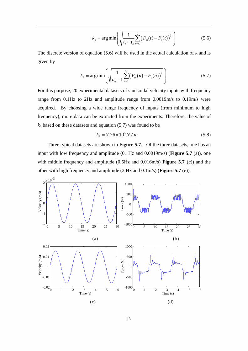
113
21
arg min ( ) ( )e
s
t
h m c
t te s
k F t F tt t
(5.6)
The discrete version of equation (5.6) will be used in the actual calculation of k and is
given by
2
1
1arg min ( ) ( )
1
en
h m c
ne
k F n F nn
(5.7)
For this purpose, 20 experimental datasets of sinusoidal velocity inputs with frequency
range from 0.1Hz to 2Hz and amplitude range from 0.0019m/s to 0.19m/s were
acquired. By choosing a wide range frequency of inputs (from minimum to high
frequency), more data can be extracted from the experiments. Therefore, the value of
kh based on these datasets and equation (5.7) was found to be
57.76 10 /hk N m (5.8)
Three typical datasets are shown in Figure 5.7. Of the three datasets, one has an
input with low frequency and amplitude (0.1Hz and 0.0019m/s) (Figure 5.7 (a)), one
with middle frequency and amplitude (0.5Hz and 0.016m/s) Figure 5.7 (c)) and the
other with high frequency and amplitude (2 Hz and 0.1m/s) (Figure 5.7 (e)).
0 5 10 15 20 25 30-2
-1
0
1
2x 10
-3
Time (s)
Vel
oci
ty (
m/s
)
0 5 10 15 20 25 30-1000
-500
0
500
1000
Fo
rce
(N)
Time (s)
(a) (b)
0 1 2 3 4 5 6-0.02
-0.01
0
0.01
0.02
Time (s)
Vel
oci
ty (
m/s
)
0 1 2 3 4 5 6-1000
-500
0
500
1000
Fo
rce
(N)
Time (s)
(c) (d)

114
0 0.5 1 1.5-0.2
-0.15
-0.1
-0.05
0
0.05
0.1
0.15
Time (s)
Vel
oci
ty (
m/s
)
0 0.5 1 1.5-2000
-1000
0
1000
2000
Fo
rce
(N)
Time (s)
(e) (f)
Figure 5.7 Sinusoidal velocity inputs and corresponding measured forces. (a), (c)
and (e) are sinusoidal velocity inputs associated with frequency-amplitude
combinations of (0.1Hz, 0.0019m/s), (0.5Hz, 0.016m/s) and (2Hz, 0.1m/s),
respectively. (b), (d) and (f) are measured forces corresponding to the inputs in (a), (c)
and (e), respectively.
Since the value of kh has been determined, the measured forces and calculated
forces based on kh can be compared. For this purpose, another two sets of data with
velocity inputs (0.4Hz, 0.012m/s) and (2Hz, 0.063m/s) are shown in Figure 5.8 (a) and
(c) respectively. The measured forces and calculated forces corresponding to the
velocity inputs in Figure 5.8 (a) and (c) are respectively presented in Figure 5.8 (b) and
(d). With the exception of the points where the terminals of the hydraulic device
experience the largest acceleration and deceleration, the measured and calculated forces
are in close agreement, which shows that the system stiffness kh has been accurately
identified.
0 2 4 6 8 10 12-0.015
-0.01
-0.005
0
0.005
0.01
0.015
Time (s)
Vel
oci
ty (
m/s
)
0 2 4 6 8 10 12
-500
0
500
Time(s)
Fo
rce
(N)
Actual
Calculated
(a) (b)
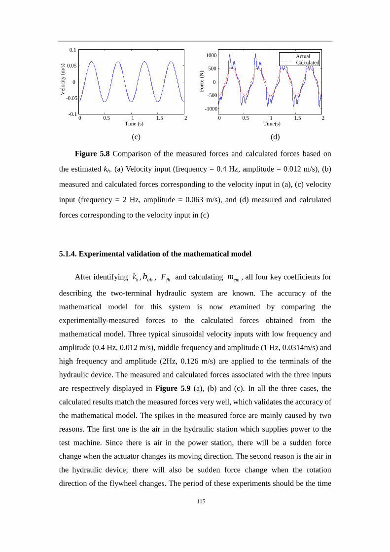
115
0 0.5 1 1.5 2-0.1
-0.05
0
0.05
0.1
Time (s)
Vel
oci
ty (
m/s
)
0 0.5 1 1.5 2
-1000
-500
0
500
1000
Time(s)
Fo
rce
(N)
Actual
Calculated
(c) (d)
Figure 5.8 Comparison of the measured forces and calculated forces based on
the estimated kh. (a) Velocity input (frequency = 0.4 Hz, amplitude = 0.012 m/s), (b)
measured and calculated forces corresponding to the velocity input in (a), (c) velocity
input (frequency = 2 Hz, amplitude = 0.063 m/s), and (d) measured and calculated
forces corresponding to the velocity input in (c)
5.1.4. Experimental validation of the mathematical model
After identifying hk , ahb , fhF and calculating emm , all four key coefficients for
describing the two-terminal hydraulic system are known. The accuracy of the
mathematical model for this system is now examined by comparing the
experimentally-measured forces to the calculated forces obtained from the
mathematical model. Three typical sinusoidal velocity inputs with low frequency and
amplitude (0.4 Hz, 0.012 m/s), middle frequency and amplitude (1 Hz, 0.0314m/s) and
high frequency and amplitude (2Hz, 0.126 m/s) are applied to the terminals of the
hydraulic device. The measured and calculated forces associated with the three inputs
are respectively displayed in Figure 5.9 (a), (b) and (c). In all the three cases, the
calculated results match the measured forces very well, which validates the accuracy of
the mathematical model. The spikes in the measured force are mainly caused by two
reasons. The first one is the air in the hydraulic station which supplies power to the
test machine. Since there is air in the power station, there will be a sudden force
change when the actuator changes its moving direction. The second reason is the air in
the hydraulic device; there will also be sudden force change when the rotation
direction of the flywheel changes. The period of these experiments should be the time

116
between two spike forces instead of the oscillation caused by spike forces.
0 1 2 3 4 5 6 7 8 9 10
-1000
-500
0
500
1000
Time(s)
Fo
rce
(N)
Actual
Calculated
(a)
0 0.5 1 1.5 2 2.5 3 3.5 4-1000
-500
0
500
1000
Time(s)
Fo
rce
(N)
Actual
Calculated
(b)
0 0.5 1 1.5 2 2.5 3 3.5 4-2000
-1000
0
1000
2000
Time(s)
Fo
rce
(N)
Actual
Calculated
(c)
Figure 5.9 The comparison of measured forces and calculated forces using the
mathematical model. (a) comparison between measured and calculated forces with a
velocity input of low frequency and amplitude (0.4 Hz, 0.012 m/s), (b) comparison
between measured and calculated forces with an input of middle frequency and
amplitude (1 Hz, 0.0314m/s), and (c) comparison between measured and calculated
forces with an input of high frequency and amplitude (2Hz, 0.126 m/s).

117
5.2. Experimental identification for the inverse screw system
with nylon adaptive flywheel
5.2.1. Experimental Set-up
Control board
Load cell
Inverse screw system
with nylon flywheel
Actuator
Cross beam
Sliding track
Figure 5.10 Experimental rig of inverse screw system with nylon flywheel
From equation (3.38), the mathematical model of this system can be described by four
key parameters ki, ci, fi and enm . An accurate mathematical model of this system can be
obtained after the determination of the four parameters. However, the same situation
occurs as mentioned in section 5.1; parameters ki, ci, and fi cannot be directly
calculated or measured, which requires experimental identification.
The Letry electro hydraulic servo fatigue test machine PLN-20 was used for this
experiment. The experimental rig of inverse screw system with nylon adaptive
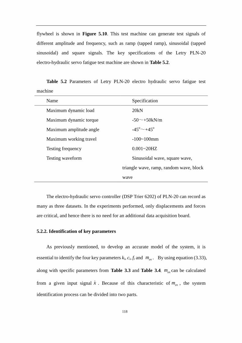
118
flywheel is shown in Figure 5.10. This test machine can generate test signals of
different amplitude and frequency, such as ramp (tapped ramp), sinusoidal (tapped
sinusoidal) and square signals. The key specifications of the Letry PLN-20
electro-hydraulic servo fatigue test machine are shown in Table 5.2.
Table 5.2 Parameters of Letry PLN-20 electro hydraulic servo fatigue test
machine
Name Specification
Maximum dynamic load 20kN
Maximum dynamic torque -50~+50kN/m
Maximum amplitude angle -45o~+45
o
Maximum working travel -100~100mm
Testing frequency 0.001~20HZ
Testing waveform Sinusoidal wave, square wave,
triangle wave, ramp, random wave, block
wave
The electro-hydraulic servo controller (DSP Trier 6202) of PLN-20 can record as
many as three datasets. In the experiments performed, only displacements and forces
are critical, and hence there is no need for an additional data acquisition board.
5.2.2. Identification of key parameters
As previously mentioned, to develop an accurate model of the system, it is
essential to identify the four key parameters ki, ci, fi and enm . By using equation (3.33),
along with specific parameters from Table 3.3 and Table 3.4, enm can be calculated
from a given input signal x . Because of this characteristic of enm , the system
identification process can be divided into two parts.

119
First, assuming that there is a sinusoidal signal input with amplitude 0.005m and
frequency 2Hz, the corresponding equivalent mass can be represented as shown in
Figure 5.11. Additional experimental data can be found in Appendix B.
0 0.2 0.4 0.6 0.8 1
-5
0
5x 10
-3
Time (s)
Dis
pla
cem
ent
(m)
0 0.2 0.4 0.6 0.8 1
580
600
620
640
660
680
700
720
Time (s)
Eq
uiv
alen
t m
ass
(kg
)
(a) (b)
Figure 5.11 Theoretical input (a) and corresponding calculated equivalent mass
(b)
As shown in Figure 5.11, because the sinusoidal signal input generates a variable
centrifugal force, this in turn changes the equivalent mass of the flywheel, as shown in
Figure 5.11 (b).
For the remaining parameter identification, many factors will affect the remaining
three parameters such as the material of the inverse screw system, the set-up of
experimental rig and the lubrication condition. Therefore, these three parameters
cannot be accurately theoretically calculated and experimental data are needed to
determine the three parameters. The most accurate values of these parameters can be
determined from the following equation:
21
{ , , } arg min ( ) ( )ei
si
t
i i i mi ti
t tei si
f c k F t F tt t
(5.9)
where ( )miF t is the measured force, ( )ciF t is the theoretically calculated force from
equation (5.9), sit is the start time of data recording, and eit is the end time. Since the
data are discrete, the above criterion can be rewritten as
2
1
1{ , , } arg min ( ) ( )
1
ein
i i i mi ti
nei
f c k F n F nn
(5.10)

120
where ( )miF n is the measured force and ( )ciF n is the theoretically calculated force
using equation (5.10) at sampling point n, and nei is the last sampling point of a dataset.
By using 21 datasets of sinusoidal inputs with frequency range from 0.1Hz to 5Hz and
amplitude range from 0.005m to 0.015mm, parameters fi, ki and ci were estimated as
7600ic Ns/m, 80if N, 61.97 10ik N/m (5.11)
The calculated forces based on the three estimated parameters and measured
forces are compared in Figure 5.12. The sinusoidal displacement inputs are plotted in
Figure 5.12 (a), (c) and (e) with frequency 0.1Hz, amplitude 0.005m , frequency 0.5Hz,
amplitude 0.01m and frequency 2Hz, amplitude 0.005m, respectively. The measured
force and calculated force corresponding to inputs in Figure 5.12 (a), (c) and (e) are
presented in Figure 5.12 (b), (d) and (f). As shown, the accuracy of the estimated c, f
and k can be clearly verified by the close agreement between the measured and
calculated forces.
0 5 10 15 20-5
0
5x 10
-3
Time (s)
Dis
pla
cem
ent
(m)
0 5 10 15 20-500
0
500
Time(s)
Forc
e(N
)
Actual
Calculated
(a) (b)
0 1 2 3 4-0.01
-0.005
0
0.005
0.01
Time (s)
Dis
pla
cem
ent
(m)
0 0.5 1 1.5 2 2.5 3 3.5 4
-500
0
500
Time(s)
Fo
rce(
N)
Actual
Calculated
(c) (d)
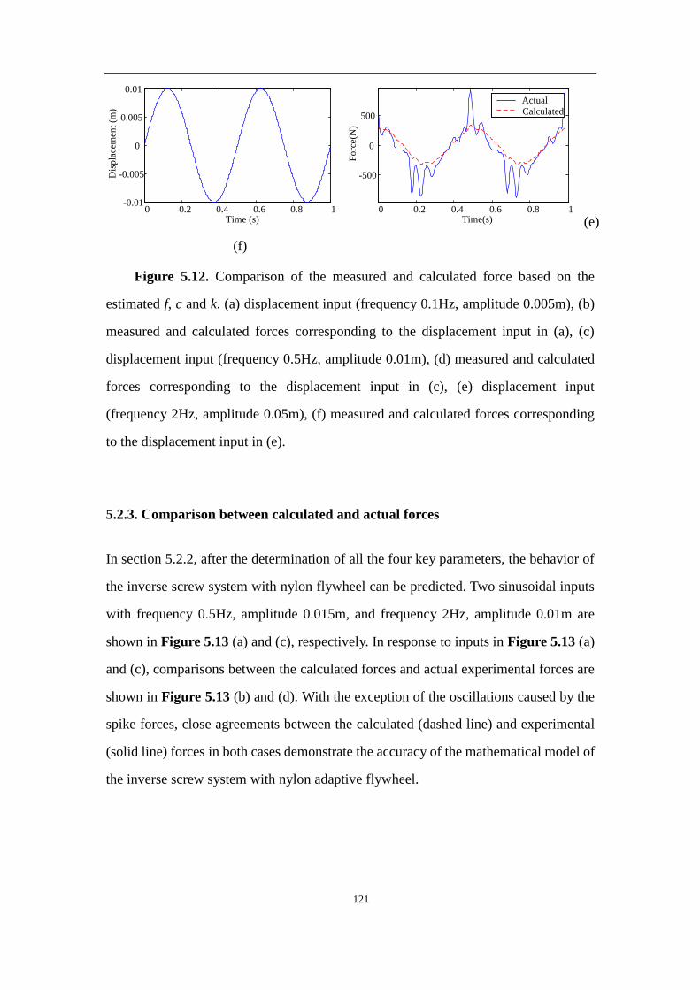
121
0 0.2 0.4 0.6 0.8 1-0.01
-0.005
0
0.005
0.01
Time (s)
Dis
pla
cem
ent
(m)
0 0.2 0.4 0.6 0.8 1
-500
0
500
Time(s)
Fo
rce(
N)
Actual
Calculated
(e)
(f)
Figure 5.12. Comparison of the measured and calculated force based on the
estimated f, c and k. (a) displacement input (frequency 0.1Hz, amplitude 0.005m), (b)
measured and calculated forces corresponding to the displacement input in (a), (c)
displacement input (frequency 0.5Hz, amplitude 0.01m), (d) measured and calculated
forces corresponding to the displacement input in (c), (e) displacement input
(frequency 2Hz, amplitude 0.05m), (f) measured and calculated forces corresponding
to the displacement input in (e).
5.2.3. Comparison between calculated and actual forces
In section 5.2.2, after the determination of all the four key parameters, the behavior of
the inverse screw system with nylon flywheel can be predicted. Two sinusoidal inputs
with frequency 0.5Hz, amplitude 0.015m, and frequency 2Hz, amplitude 0.01m are
shown in Figure 5.13 (a) and (c), respectively. In response to inputs in Figure 5.13 (a)
and (c), comparisons between the calculated forces and actual experimental forces are
shown in Figure 5.13 (b) and (d). With the exception of the oscillations caused by the
spike forces, close agreements between the calculated (dashed line) and experimental
(solid line) forces in both cases demonstrate the accuracy of the mathematical model of
the inverse screw system with nylon adaptive flywheel.

122
0 1 2 3 4-0.015
-0.01
-0.005
0
0.005
0.01
0.015
Time (s)
Dis
pla
cem
ent
(m)
0 0.5 1 1.5 2 2.5 3 3.5 4
-500
0
500
Time(s)
Fo
rce(
N)
Actual
Calculated
(a) (b)
0 0.2 0.4 0.6 0.8 1-0.01
-0.005
0
0.005
0.01
Time (s)
Dis
pla
cem
ent
(m)
0 0.2 0.4 0.6 0.8 1-2000
-1000
0
1000
2000
Time(s)
Fo
rce(
N)
Actual
Calculated
(c) (d)
Figure 5.13. Comparison between the actual and calculated force, based on the
mathematical model: (a) sinusoidal input with frequency 0.5Hz and amplitude 0.015m,
(b) comparison between actual and calculated force corresponding to the sinusoidal
input in (a), (c) sinusoidal input with frequency 2Hz and amplitude 0.01m, (d)
comparison of the actual and calculated force corresponding to the sinusoidal input in
(c)
To better observe the behavior of the nylon adaptive flywheel, two additional
experiments were performed. First, experiments under three situations were carried out:
maximum, minimum and variable (spring-driven) slider position, respectively. By
using foamed plastic, the location of the sliders in the slots can be fixed at the maximum
radius (the longest distance from the rotation center) and at the minimum radius (the
shortest distance from the rotation center). The comparison is shown in Figure 5.14
with sinusoidal input of frequency 1Hz and amplitude 0.005m.
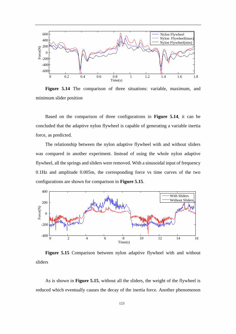
123
0 0.2 0.4 0.6 0.8 1 1.2 1.4 1.6 1.8
-600
-400
-200
0
200
400
600
Fo
rce(
N)
Time(s)
Nylon FlywheelNylon Flywheel(max)
Nylon Flywheel(min)
Figure 5.14 The comparison of three situations: variable, maximum, and
minimum slider position
Based on the comparison of three configurations in Figure 5.14, it can be
concluded that the adaptive nylon flywheel is capable of generating a variable inertia
force, as predicted.
The relationship between the nylon adaptive flywheel with and without sliders
was compared in another experiment. Instead of using the whole nylon adaptive
flywheel, all the springs and sliders were removed. With a sinusoidal input of frequency
0.1Hz and amplitude 0.005m, the corresponding force vs time curves of the two
configurations are shown for comparison in Figure 5.15.
0 2 4 6 8 10 12 14 16-400
-200
0
200
400
Time(s)
Fo
rce(
N)
With Sliders
Without Sliders
Figure 5.15 Comparison between nylon adaptive flywheel with and without
sliders
As is shown in Figure 5.15, without all the sliders, the weight of the flywheel is
reduced which eventually causes the decay of the inertia force. Another phenomenon

124
that can be observed from the 8th
to the 14th
second in Figure 5.15 is that the adaptive
flywheel shows a certain ability to suppress the spike force which is caused by the
hydraulic station and transmission backlash in the inverse screw.
5.3. Two-terminal hydraulic system with rectifier
In this chapter, experiments are carried out to verify the mathematical model of
two-terminal devices. The close agreement between the experimental results and the
calculated results based on the model indicates that the model is accurate. However, in
all these experiments, there is always the inevitable problem of spike in the measured
force. In the previous experiments, some key parameters were identified through
experimental data. Even if most of the spikes in the data were eliminated during
identification, the results will still be affected by the presence of the spikes. By
reducing the spikes in the experiments, the accuracy of the key parameters will be
improved, which leads to a more accurate mathematical model for the two-terminal
hydraulic system.
As mentioned before, the spikes in the experiments are mainly caused by the
hydraulic station and backlash in the two-terminal system. For a hydraulic station, the
characteristics of the system are fixed after manufacture and calibration, which
implies that it is almost impossible to eliminate the spikes by adjusting the hydraulic
station. The only feasible way to reduce the spikes is to minimize the effect caused by
backlash. Through improving the manufacturing precision, the transmission backlash
in the inverse-screw system can be reduced. However, the cost of this two-terminal
system will then increase dramatically.
For a hydraulic system, due to air in the hydraulic oil, the existence of backlash
is inevitable. The air in the hydraulic system can be reduced by multiple ways, but
they usually require an auxiliary device and a lot of time. Therefore, when the air in
the hydraulic system reaches a relative low level, it will be much more difficult to
minimize the backlash by further reducing the air in the hydraulic system. In the

125
experiments performed herein, the spike force always appears when there is a change
in movement direction. By adding a hydraulic rectifier to force the hydraulic motor to
rotate in a single direction instead of constantly changing direction, the spike force
can be reduced effectively. The prototype of the two-terminal hydraulic system with
rectifier is shown in Figure 5.16.
4
32
5
1
Figure 5.16 prototype of two-terminal hydraulic system with rectifier (Note:
1-terminal one 2- hydraulic motor 3-flywheel 4-terminal two 5-hydraulic rectifier)
The parameters of the new two-terminal hydraulic system with rectifier can be
found in Table 5.3
Table 5.3 Specific parameters of the new two-terminal hydraulic system
No Name Notation Specification
1 Travel of the piston 0.3 m
2 Maximum pressure 8 MPa
3 Cross-section area of the cylinder A 0.00146 m2
4 Displacement of the motor H 1.107210-6
m3/rad
As mentioned in chapter 3, in order to obtain a higher changing ratio, a
light-density, high-strength material, nylon in this case, is used to manufacture the
adaptive flywheel. However, due to its light weight, it will eventually lead to an
insufficient inertial force in future applications with a two-terminal hydraulic system.

126
By re-designing the parameters of the nylon adaptive flywheel, the flywheel can
generate enough inertial force for the two-terminal hydraulic system with rectifier.
The schematic diagram of new nylon adaptive flywheel is shown Figure 5.17. The
design of the new adaptive flywheel is identical to the design in Chapter 3. The only
difference between these two designs is the actual value of those key parameters.
Rr
dr
rr
rr
Lr
lr
l
C
C C-C
dr
Figure 5.17 Schematic diagram of new nylon adaptive flywheel
The key parameters of this new adaptive flywheel can be found in Table 5.4
Table 5.4 Specific parameters of the new nylon adaptive flywheel
Name Notation Specification
Outer radius of flywheel
Thickness of nylon disk
Rr
Tr
0.075m
0.033m
Distance between hole and rotation
center
Lr 0.056m
Radius of inner circle rr1 0.01m
Radius of holes in flywheel rr2 0.013m
Diameter of slots in flywheel dr 0.025m
Length of slots lr1 0.053m

127
Radius of sliders
Length of sliders
Mass of slider
Density of PA66
Stiffness of spring
rr3
lr2
msr
ρ
ksr
0.012m
0.022m
0.078kg
1150kg/m3
120N/m
The Letry electro hydraulic servo fatigue test machine PLN-20 was again used in
the experiments. The experimental rig of the two-terminal hydraulic system with
rectifier is shown in Figure 5.18. The specific parameters of this test machine can be
found in Table 5.2.
Control board
Load cell
Two-terminal
hydraulic system
with rectifier
Actuator
Cross beam
Sliding track
Figure 5.18 Experimental rig of two-terminal hydraulic system with rectifier
The first two sets of experiments were conducted without the adaptive flywheel.
The only difference in operating condition is with or without the hydraulic
rectifier. Through these experiments, the effect caused by the rectifier can be isolated

128
and verified. The results are shown in Figure 5.19. Additional experimental data can
be found in Appendix B.
0 2 4 6 8 10 12-0.05
-0.04
-0.03
-0.02
-0.01
0
0.01
0.02
0.03
0.04
0.05
Time (s)
Am
pli
tude
(m)
0 2 4 6 8 10 12-800
-600
-400
-200
0
200
400
600
800
Time(s)F
orc
e(N
)
Without rectifier
With rectifier
(a) (b)
Figure 5.19 Comparison of two-terminal hydraulic system with and without
rectifier: (a) Sinusoidal input (frequency = 0.4Hz, and amplitude = 0.05m), and (b)
Measured force of two-terminal hydraulic system with and without rectifier.
Figure 5.19 shows the comparison between the two-terminal hydraulic system
with and without rectifier, and shows that the spike forces are smaller when the
rectifier is applied. The results validate the effectiveness of rectifier in spike
reduction.
By substituting equations (3.19)-(3.24) with the specific parameters given in
Table 5.4, the moment of inertia of the new adaptive nylon flywheel afrI can be
calculated. Based on equation (3.11) and Table 5.3, the equivalent mass of the new
adaptive nylon flywheel erm can also be determined.
The same identification strategy as outlined in section 4.1 and 4.2 was applied to
identify the key parameters for the new hydraulic system with rectifier. The three key
parameters can be identified by:
21
{ , , } arg min ( ) ( )er
sr
t
r r r mr tr
t ter sr
f c k F t F tt t
(5.12)
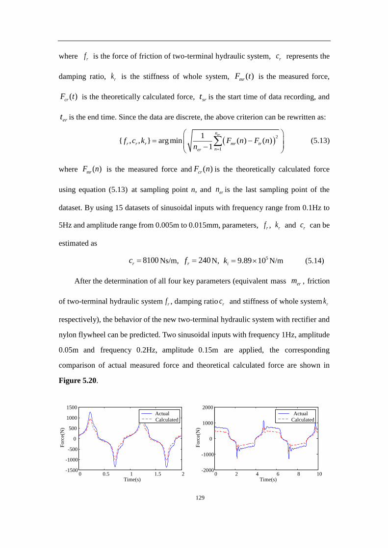
129
where rf is the force of friction of two-terminal hydraulic system, rc represents the
damping ratio, rk is the stiffness of whole system, ( )mrF t is the measured force,
( )crF t is the theoretically calculated force, srt is the start time of data recording, and
ert is the end time. Since the data are discrete, the above criterion can be rewritten as:
2
1
1{ , , } arg min ( ) ( )
1
ern
r r r mr tr
ner
f c k F n F nn
(5.13)
where ( )mrF n is the measured force and ( )crF n is the theoretically calculated force
using equation (5.13) at sampling point n, and ern is the last sampling point of the
dataset. By using 15 datasets of sinusoidal inputs with frequency range from 0.1Hz to
5Hz and amplitude range from 0.005m to 0.015mm, parameters, rf , rk and rc can be
estimated as
8100rc Ns/m, 240rf N, 59.89 10ik N/m (5.14)
After the determination of all four key parameters (equivalent mass erm , friction
of two-terminal hydraulic system rf , damping ratio rc and stiffness of whole system rk
respectively), the behavior of the new two-terminal hydraulic system with rectifier and
nylon flywheel can be predicted. Two sinusoidal inputs with frequency 1Hz, amplitude
0.05m and frequency 0.2Hz, amplitude 0.15m are applied, the corresponding
comparison of actual measured force and theoretical calculated force are shown in
Figure 5.20.
0 0.5 1 1.5 2-1500
-1000
-500
0
500
1000
1500
Time(s)
Fo
rce(
N)
Actual
Calculated
0 2 4 6 8 10
-2000
-1000
0
1000
2000
Time(s)
Fo
rce(
N)
Actual
Calculated
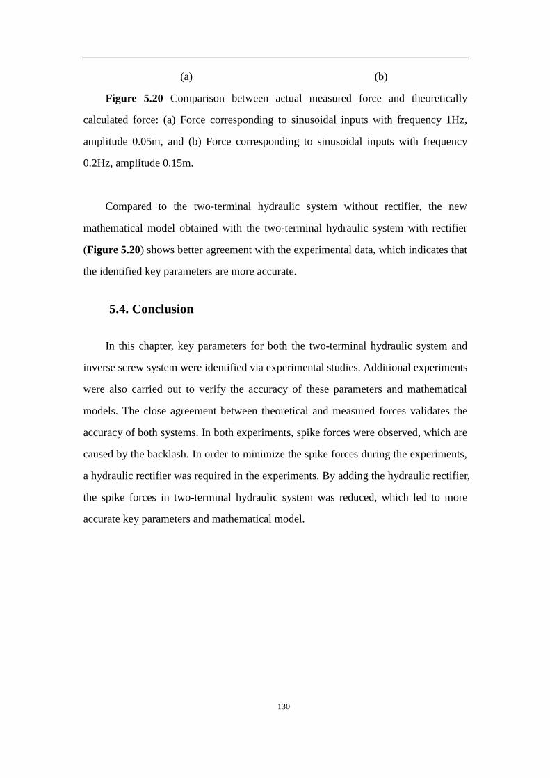
130
(a) (b)
Figure 5.20 Comparison between actual measured force and theoretically
calculated force: (a) Force corresponding to sinusoidal inputs with frequency 1Hz,
amplitude 0.05m, and (b) Force corresponding to sinusoidal inputs with frequency
0.2Hz, amplitude 0.15m.
Compared to the two-terminal hydraulic system without rectifier, the new
mathematical model obtained with the two-terminal hydraulic system with rectifier
(Figure 5.20) shows better agreement with the experimental data, which indicates that
the identified key parameters are more accurate.
5.4. Conclusion
In this chapter, key parameters for both the two-terminal hydraulic system and
inverse screw system were identified via experimental studies. Additional experiments
were also carried out to verify the accuracy of these parameters and mathematical
models. The close agreement between theoretical and measured forces validates the
accuracy of both systems. In both experiments, spike forces were observed, which are
caused by the backlash. In order to minimize the spike forces during the experiments,
a hydraulic rectifier was required in the experiments. By adding the hydraulic rectifier,
the spike forces in two-terminal hydraulic system was reduced, which led to more
accurate key parameters and mathematical model.

131
6. Application of hydraulic two-terminal device with
adaptive flywheel to suspension system
In Chapter 4, three different suspension systems were evaluated under ideal
conditions. In this chapter, instead of an ideal hydraulic two-terminal device, a
modified model of the hydraulic two-terminal device (referred to as an “actual”
hydraulic two-terminal device) is applied to the suspension system. The reason for
this approach is to be able to understand the factors that affect the performance of the
proposed designed systems. The key parameters of the hydraulic system have been
identified in Chapter 5. Therefore, another two suspension systems are introduced,
which are the suspension system consisting of a two-terminal device without adaptive
flywheel (suspension system A) and suspension system consisting of a two-terminal
device with adaptive flywheel (suspension system B). Performance criteria are
applied to evaluate these two suspension systems, and comparisons are carried out
between them and a traditional suspension system with no flywheel. Finally, the
performance of suspension system B with different changing ratio is discussed, and an
optimal changing ratio is determined under certain circumstances.
6.1. Mathematical models for the suspension systems
In this chapter, rather than the two-terminal inverse screw system, the
two-terminal hydraulic system is chosen for two reasons. First, since the ideal
two-terminal hydraulic system was chosen for simulation in chapter 4, a two-terminal
hydraulic system is also chosen here for consistence and fair comparison. The second
reason is the application environment. For application to a suspension system, the
frequency of the vibrations can be quite high, which will lead to abrasion of a screw
transmission. Under this situation, the inverse screw system can be damaged in a short

132
period of time.
To isolate the behavior of the adaptive flywheel, a new suspension system model
is required. Therefore, as shown in Figure 6.1, suspension system A is introduced.
Compared to a traditional suspension system, a hydraulic two-terminal system must
also be added between the tire and vehicle body in suspension system A.
M
KC
X2
X1
CtKt
X3
Mt
kh
bah
xk
Figure 6.1 Suspension system A
From Figure 6.1, the mathematical model of suspension system A can be written
as:
3 3 2 3 2 3 2
2 2 1 2 1 3 2 3 2
3 2 3 2
( ) ( ) ( ) 0
( ) ( ) ( ) ( ) 0
( ) sgn( )
ah k
t t t h k
h k ah k fh
MX K X X C X X b X X x
M X K X X C X X K X X C X X k x
k x b X X x F X X
(6.1)
In equation (6.1), M is the weight of quarter car and one passenger, K
represents the stiffness of suspension system, C is the damping ratio of suspension
system, ahb is the damping ratio of two-terminal hydraulic system, hk is the stiffness of
the two-terminal hydraulic system, and kx is the elastic deformation of the
two-terminal hydraulic system, tK is the stiffness of the tire, tC is the damping
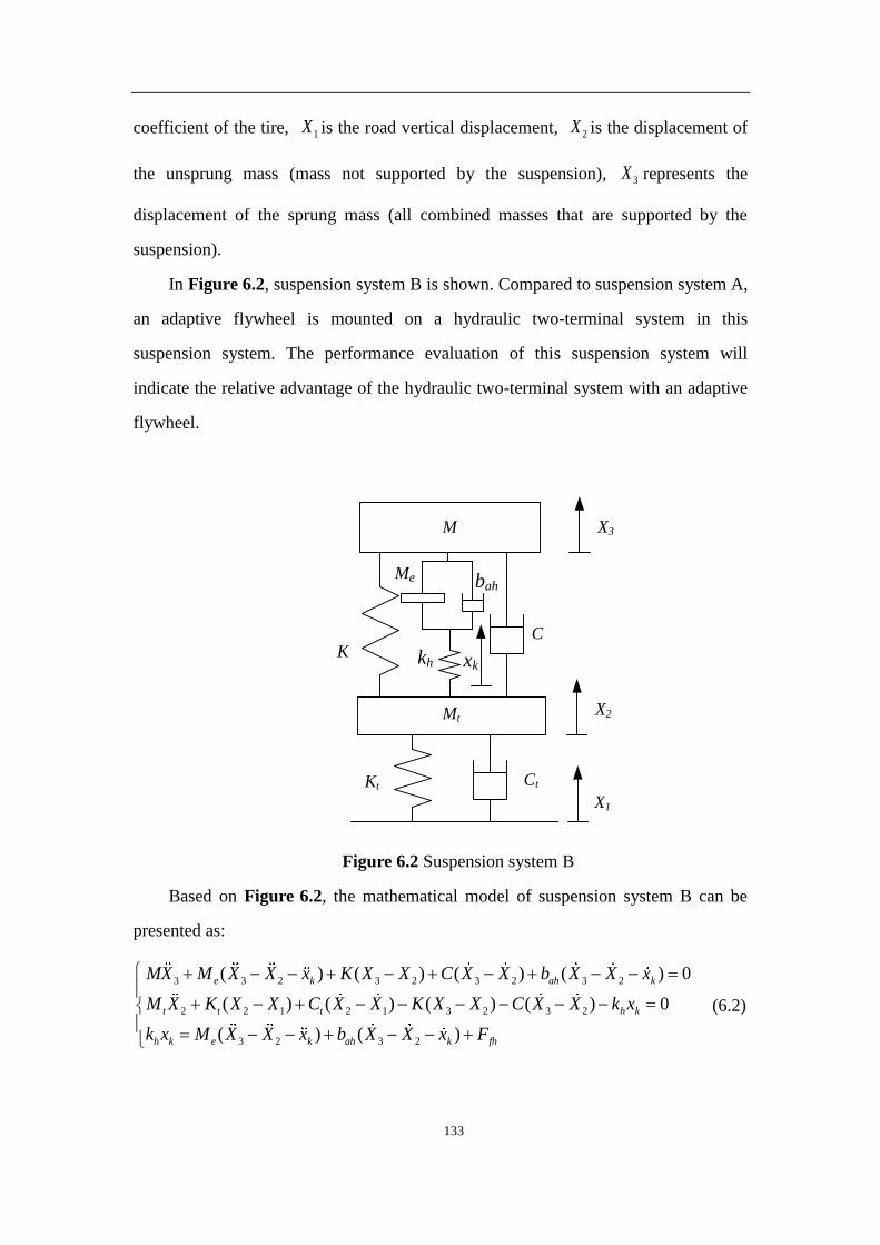
133
coefficient of the tire, 1X is the road vertical displacement, 2X is the displacement of
the unsprung mass (mass not supported by the suspension), 3X represents the
displacement of the sprung mass (all combined masses that are supported by the
suspension).
In Figure 6.2, suspension system B is shown. Compared to suspension system A,
an adaptive flywheel is mounted on a hydraulic two-terminal system in this
suspension system. The performance evaluation of this suspension system will
indicate the relative advantage of the hydraulic two-terminal system with an adaptive
flywheel.
M
KC
X2
X1
CtKt
X3
Mt
kh
Me bah
xk
Figure 6.2 Suspension system B
Based on Figure 6.2, the mathematical model of suspension system B can be
presented as:
3 3 2 3 2 3 2 3 2
2 2 1 2 1 3 2 3 2
3 2 3 2
( ) ( ) ( ) ( ) 0
( ) ( ) ( ) ( ) 0
( ) ( )
e k ah k
t t t h k
h k e k ah k fh
MX M X X x K X X C X X b X X x
M X K X X C X X K X X C X X k x
k x M X X x b X X x F
(6.2)
134
6.2. Performance evaluation
As indicated earlier, due to the non-linearity of the adaptive flywheel, the
transfer function of suspension system B cannot be obtained in closed form. Therefore,
the same performance criteria will be introduced to evaluate suspension system A and
suspension system B as previously used, which are riding comfort, tire grip and
vehicle body deflection. The same simulation strategy as used in Chapter 4 is applied
to the performance evaluation, which implies that the static moment of inertia of the
nylon adaptive flywheel is still set at 4 2
,min 2.231 10 .afnI kg m and the other key
parameters of these two suspension systems can be obtained from equation (4.16).
The parameters of the hydraulic two-terminal system were identified in Chapter 5.
6.2.1. Riding comfort
Riding comfort is one of the most important performance criteria for a
suspension system. Due to the non-linearity of suspension system B, equation (4.12)
cannot be applied to evaluate the riding comfort of suspension system B. However,
weighted root mean square acceleration is considered as a key index to judge the riding
comfort when the velocity of the car is fixed, and this is expressed in meters per
second squared (m/𝑠2) for translational vibrations. Based on equation (4.15), the
weighted root mean square acceleration of suspension system A and B can be
determined.
Similar to Chapter 4, three different excitations are applied to simulate the road
surface, which are zero input, impulse input and sinusoidal input, respectively.
6.2.1.1. Zero input
An initial displacement of 0.05m is applied to the three suspension systems,
which are traditional suspension system, suspension system A and suspension system

135
B. Through the combination of equation (4.1), (4.15), (6.1) and (6.2), the numerical
solution of the weighted root mean square acceleration for each suspension system in
the time-domain can be calculated through Matlab. The results of this simulation are
shown in Table 6.1 as the vehicle body mass is varied.
Table 6.1 Weighted root mean square acceleration with zero input
Vehicle
body
mass
vM (kg)
Weighted
accelerations
of traditional
suspension
system
aw(m/s2)
Weighted
accelerations of
suspension
system A aw(m/s2)
Weighted
accelerations of
suspension
system B
aw(m/s2)
340 0.4656 0.3749 0.2879
350 0.4524 0.3643 0.2847
360 0.4397 0.3571 0.2813
370 0.4288 0.3493 0.2779
380 0.4154 0.3425 0.2741
390 0.3996 0.3359 0.2707
400 0.3878 0.3187 0.2671
340 350 360 370 380 390 4000.25
0.3
0.35
0.4
0.45
0.5
Wei
gh
ted
acc
eler
atio
n a
w(m
/s2)
Vehicle body mass Mv(kg)
Traditional suspension system
Suspension system ASuspension system B
Figure 6.3 Weighted root mean square acceleration with zero input

136
Figure 6.3 shows the weighted root mean square acceleration of three suspension
systems under zero input. The weighted root mean square acceleration of suspension
system B is smaller than other two suspension systems under the same vehicle body
mass, which implies that the suspension system B outperforms both traditional
suspension system and suspension system A. Compared to results in Table 4.1, the
same trends can be found in Table 6.1, with the increasing of vehicle body mass, the
riding comfort improves. However, suspension system B shows better performance
than the AFW suspension system in chapter 4 for riding comfort. Since the weighted
root mean square acceleration of suspension system A is smaller than the traditional
suspension system, which means, in addition to the adaptive flywheel, the
two-terminal hydraulic system also improves riding comfort.
6.2.1.2. Impulse input
An impulse input with amplitude of 0.05m is applied to each suspension system.
Using the same mathematical model, the results can be determined by Matlab and are
shown in Table 6.2.
Table 6.2 Weighted root mean square acceleration with impulse input
Vehicle
body
mass
vM (kg)
Weighted
accelerations of
traditional
suspension
system
Weighted
accelerations of
suspension
system A
aw(m/s2)
Weighted
accelerations of
suspension
system B
aw(m/s2)
340 0.4878 0.3728 0.2589
350 0.4684 0.3614 0.2557
360 0.4546 0.3519 0.2521
370 0.4398 0.3432 0.2487

137
380 0.4264 0.3353 0.2459
390 0.4112 0.3281 0.2427
400 0.3986 0.3216 0.2384
340 350 360 370 380 390 4000.2
0.25
0.3
0.35
0.4
0.45
0.5
Wei
ghte
d a
ccel
erat
ion a
w(m
/s2)
Vehicle body mass Mv(kg)
Traditional suspension system
Suspension system ASuspension system B
Figure 6.4 Weighted root mean square acceleration with impulse input
Figure 6.4 shows the weighted root mean square acceleration of the three
suspension systems under impulse input. The weighted root mean square
acceleration of suspension system B is the smallest of the three suspension systems
under the same vehicle body mass, which indicates that suspension system B shows
better performance than the other two suspension systems. By comparing results
between Table 4.2 and Table 6.2, the results are similar to the results under zero input.
That is, with the increase in vehicle body mass, the riding comfort improves in both
the AFW suspension system and suspension system B. However, with the
two-terminal hydraulic system, suspension system B out-performs the AFW
suspension system in riding comfort.
6.2.1.3. Sinusoidal input
To simulate a rough road situation, a sinusoidal input with wave length of 4m,

138
amplitude 0.05m and frequency 5Hz is applied to each suspension system. The results
of simulation can be found in Table 6.3
Table 6.3 Weighted root mean square acceleration with sinusoidal input
Vehicle
body
mass vM
(kg)
Weighted
accelerations of
traditional
suspension
system
Weighted
accelerations of
suspension
system A
aw(m/s2)
Weighted
accelerations of
suspension
system B
aw(m/s2)
340 1.9786 1.7453 1.8497
350 1.8498 1.6231 1.7549
360 1.7249 1.5107 1.6643
370 1.6256 1.3891 1.4989
380 1.5143 1.2797 1.3658
390 1.3983 1.1789 1.2873
400 1.2964 1.0813 1.1847
340 350 360 370 380 390 4001
1.1
1.2
1.3
1.4
1.5
1.6
1.7
1.8
1.9
2
Wei
ghte
d a
ccel
erat
ion a
w(m
/s2)
Vehicle body mass Mv(kg)
Traditional suspension system
Suspension system ASuspension system B
Figure 6.5 Weighted root mean square acceleration with sinusoidal input
As shown in Figure 6.5, with sinusoidal input, the results of the three suspension

139
systems in this case are different than with the two other inputs. Here, the weighted
root mean square acceleration of suspension system B is larger than suspension
system A, but smaller than with the traditional suspension. This result implies that
suspension system B gives the middle performance of the three chosen suspension
systems under the case of a sinusoidal input. The results in Table 4.3 show that
suspension system B is better than the AFW suspension system in riding comfort.
However, based on Table 6.3, suspension system A out-performs suspension system B.
Therefore, the better riding comfort of suspension system B is due to the two-terminal
hydraulic system.
6.2.2. Tire grip
As a key criterion to indicate the ride safety of a vehicle, tire grip index is
another important factor to evaluate the performance of a suspension system. Due to
the non-linearity of suspension system B, the tire grip index is defined as the ratio
between static and dynamic loads, which can be calculated via equation (4.21). The
same simulation strategy as used in Chapter 4 is applied to these comparison
simulations.
6.2.2.1. Zero input
An initial displacement 0.05m is applied to the three suspension systems. The
results can be found in Table 6.4.
Table 6.4 Weighted root mean square tire grip index with zero input
Vehicle body
mass vM (kg)
Weighted
tire grip index
of traditional
suspension
system wtgM
Weighted tire
grip index of
suspension system
A wtgM
Weighted tire
grip index of
suspension system
B wtgM
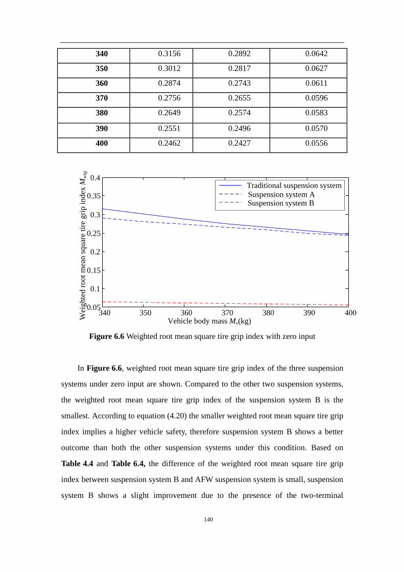
140
340 0.3156 0.2892 0.0642
350 0.3012 0.2817 0.0627
360 0.2874 0.2743 0.0611
370 0.2756 0.2655 0.0596
380 0.2649 0.2574 0.0583
390 0.2551 0.2496 0.0570
400 0.2462 0.2427 0.0556
340 350 360 370 380 390 4000.05
0.1
0.15
0.2
0.25
0.3
0.35
0.4
Vehicle body mass Mv(kg)Wei
ghte
d r
oo
t m
ean s
quar
e ti
re g
rip i
ndex
Mw
tg
Traditional suspension system
Suspension system ASuspension system B
Figure 6.6 Weighted root mean square tire grip index with zero input
In Figure 6.6, weighted root mean square tire grip index of the three suspension
systems under zero input are shown. Compared to the other two suspension systems,
the weighted root mean square tire grip index of the suspension system B is the
smallest. According to equation (4.20) the smaller weighted root mean square tire grip
index implies a higher vehicle safety, therefore suspension system B shows a better
outcome than both the other suspension systems under this condition. Based on
Table 4.4 and Table 6.4, the difference of the weighted root mean square tire grip
index between suspension system B and AFW suspension system is small, suspension
system B shows a slight improvement due to the presence of the two-terminal

141
hydraulic system.
6.2.2.2. Impulse input
An impulse input with amplitude of 0.05m is applied to each suspension system.
The results are shown in Table 6.5.
Table 6.5 Weighted root mean square tire grip index with impulse input
Vehicle body
mass vM (kg)
Weighted
tire grip index
of traditional
suspension
system wtgM
Weighted tire
grip index of
suspension system
A wtgM
Weighted tire
grip index of
suspension system
B wtgM
340 0.3879 0.3774 0.1139
350 0.3624 0.3541 0.1085
360 0.3412 0.3307 0.1027
370 0.3208 0.3119 0.0959
380 0.3001 0.2907 0.0897
390 0.2814 0.2716 0.0851
400 0.2628 0.2546 0.0804

142
340 350 360 370 380 390 4000.05
0.1
0.15
0.2
0.25
0.3
0.35
0.4
Vehicle body mass Mv(kg)Wei
ghte
d r
oot
mea
n s
quar
e ti
re g
rip i
ndex
Mw
tgTraditional suspension system
Suspension system ASuspension system B
Figure 6.7 Weighted root mean square tire grip index with impulse input
Figure 6.7 shows the weighted root mean square tire grip index of three
suspension systems with an impulse input. Since the weighted root mean square tire
grip index of suspension system B is still the smallest of all three suspension systems
under same vehicle body mass, it follows that it out-performs the suspension system A
and the traditional suspension system. From Table 4.5 in chapter 4 and Table 6.5,
the same results as zero input can be found, suspension system B also shows a slight
improvement over the AFW suspension system due to the two-terminal hydraulic
system.
6.2.2.3. Sinusoidal input
A sinusoidal input with wave length of 4m, amplitude of 0.05m and a frequency
of 5Hz is applied to each suspension system. The results are shown in Table 6.6.
Table 6.6 Weighted root mean square tire grip index with sinusoidal input
Vehicle body Weighted Weighted tire Weighted tire
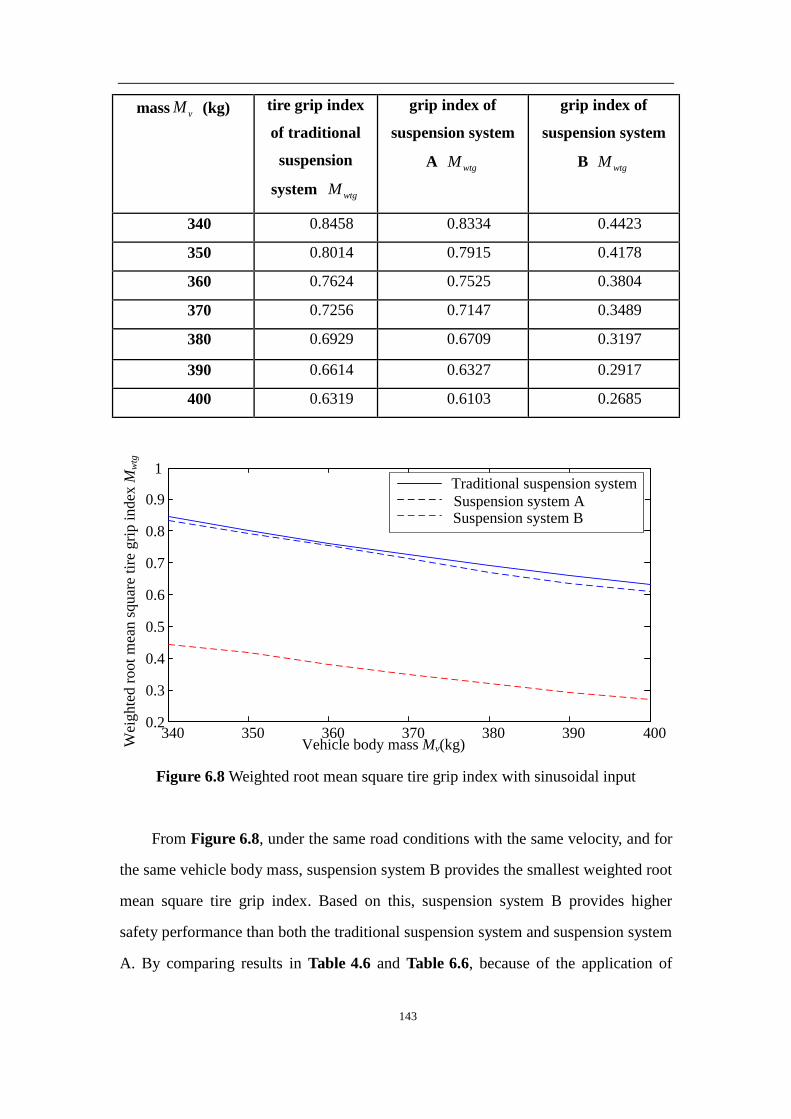
143
mass vM (kg) tire grip index
of traditional
suspension
system wtgM
grip index of
suspension system
A wtgM
grip index of
suspension system
B wtgM
340 0.8458 0.8334 0.4423
350 0.8014 0.7915 0.4178
360 0.7624 0.7525 0.3804
370 0.7256 0.7147 0.3489
380 0.6929 0.6709 0.3197
390 0.6614 0.6327 0.2917
400 0.6319 0.6103 0.2685
340 350 360 370 380 390 4000.2
0.3
0.4
0.5
0.6
0.7
0.8
0.9
1
Vehicle body mass Mv(kg)Wei
ghte
d r
oot
mea
n s
quar
e ti
re g
rip i
ndex
Mw
tg
Traditional suspension system
Suspension system ASuspension system B
Figure 6.8 Weighted root mean square tire grip index with sinusoidal input
From Figure 6.8, under the same road conditions with the same velocity, and for
the same vehicle body mass, suspension system B provides the smallest weighted root
mean square tire grip index. Based on this, suspension system B provides higher
safety performance than both the traditional suspension system and suspension system
A. By comparing results in Table 4.6 and Table 6.6, because of the application of

144
two-terminal hydraulic system, suspension system B shows better performance than
the AFW suspension system. However, the improvement of the suspension system
performance is quite small.
6.2.3. Vehicle body deflection
The last performance criterion is the vehicle body deflection. Because of the
non-linearity of suspension system B, equation (4.26) is introduced to calculate
weighted root mean square vehicle body deflection for each suspension system.
Similar to the simulations of riding comfort and tire grip index, three excitations will
be applied to simulate different road situations.
6.2.3.1. Zero input
An initial displacement 0.05m is applied on the three suspension systems. The
results are shown in Table 6.7.
Table 6.7 Weighted root mean square vehicle body deflection with zero input
Vehicle body mass
vM (kg)
vehicle body
deflections of
traditional
suspension
system Dfw(m)
Weighted vehicle
body deflections of
suspension system
A Dfw(m)
Weighted vehicle
body deflections of
suspension system
B Dfw(m)
340 0.0035 0.0021 0.0021
350 0.0035 0.0021 0.0021
360 0.0035 0.0021 0.0021
370 0.0035 0.0021 0.0020
380 0.0034 0.0020 0.0020
390 0.0034 0.0020 0.0020
400 0.0034 0.0020 0.0020

145
340 350 360 370 380 390 4000
0.5
1
1.5
2
2.5
3
3.5
4x10
-3
Vehicle body mass Mv(kg)
Wei
gh
ted
v
ehic
le b
od
y d
efle
ctio
ns
Dfw
(m
)
Traditional suspension system
Suspension system ASuspension system B
Figure 6.9 Weighted root mean square vehicle body deflection with zero input
Based on Figure 6.9, suspension system A and B show a smaller weighted root
mean square vehicle body deflection than the traditional suspension system under
zero input. However, the weighted root mean square vehicle body deflection of
suspension system A and B are almost identical. This result implies that the proposed
suspension system B shows no improvement compared to suspension system A,
which also indicates that the adaptive flywheel shows no effect on the vehicle body
deflection. Based on Table 4.7 in chapter 4 and Table 6.7, suspension system B
out-performs the AFW suspension system. However, suspension system A and
suspension system B show almost identical results. Therefore, the improvement of
suspension system B in vehicle body deflection is due to the two-terminal hydraulic
system.
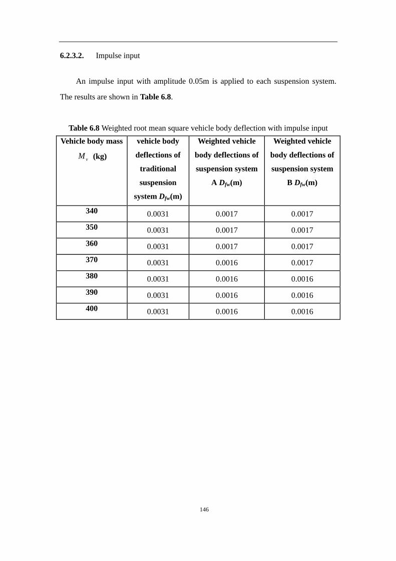
146
6.2.3.2. Impulse input
An impulse input with amplitude 0.05m is applied to each suspension system.
The results are shown in Table 6.8.
Table 6.8 Weighted root mean square vehicle body deflection with impulse input
Vehicle body mass
vM (kg)
vehicle body
deflections of
traditional
suspension
system Dfw(m)
Weighted vehicle
body deflections of
suspension system
A Dfw(m)
Weighted vehicle
body deflections of
suspension system
B Dfw(m)
340 0.0031 0.0017 0.0017
350 0.0031 0.0017 0.0017
360 0.0031 0.0017 0.0017
370 0.0031 0.0016 0.0017
380 0.0031 0.0016 0.0016
390 0.0031 0.0016 0.0016
400 0.0031 0.0016 0.0016

147
340 350 360 370 380 390 4000
0.5
1
1.5
2
2.5
3
3.5
4x10
-3
Vehicle body mass Mv(kg)
Wei
gh
ted
v
ehic
le b
od
y d
efle
ctio
ns
Dfw
(m
)
Traditional suspension system
Suspension system ASuspension system B
Figure 6.10 Weighted root mean square vehicle body deflection with impulse input
From Figure 6.10, the same results can be found as for the case of zero input.
The weighted root mean square vehicle body deflection of suspension system A and B
are almost identical, which is smaller than for the traditional suspension system. This
result indicates that there is almost no performance difference for suspension system
A and B; the adaptive flywheel shows no effect on vehicle body deflection under
impulse input. By comparing Table 4.8 in chapter 4 and Table 6.8, the same results
under zero input can be found. Because of the application of the two-terminal
hydraulic system, Suspension system B shows better performance than the traditional
suspension system.
6.2.3.3. Sinusoidal input
A sinusoidal input with wave length 4m, amplitude 0.05m and frequency 5Hz is
applied to each suspension system. The results are shown in Table 6.9.
Table 6.9 Weighted root mean square vehicle body deflection with sinusoidal input

148
Vehicle body mass
vM (kg)
vehicle body
deflections of
traditional
suspension
system Dfw(m)
Weighted vehicle
body deflections of
suspension system
A Dfw(m)
Weighted vehicle
body deflections of
suspension system
B Dfw(m)
340 0.0096 0.0077 0.0137
350 0.0095 0.0076 0.0132
360 0.0093 0.0074 0.0128
370 0.0091 0.0071 0.0122
380 0.0090 0.0071 0.0118
390 0.0088 0.0070 0.0113
400 0.0087 0.0069 0.0109
340 350 360 370 380 390 4000.006
0.007
0.008
0.009
0.01
0.011
0.012
0.013
0.014
Vehicle body mass Mv(kg)
Wei
gh
ted
v
ehic
le b
od
y d
efle
ctio
ns
Dfw
(m
)
Traditional suspension system
Suspension system ASuspension system B
Figure 6.11 Weighted root mean square vehicle body deflection with sinusoidal input
Figure 6.11 shows the weighted root mean square vehicle body deflection of the
three different suspension systems with sinusoidal input. The weighted root mean

149
square vehicle body deflection of suspension system B is bigger than other two
suspension systems, which implies that in this case, the traditional suspension system
and the suspension system A show better results than the suspension system B.
Based on the results of chapter 4 and Table 6.9, the same trend can be found in all
the suspension systems. With a higher vehicle body mass, the weighted root mean
square vehicle body deflection is smaller. Suspension system B shows slightly better
performance than the AFW suspension system, but worse performance than the
traditional suspension systems. Therefore, the two-terminal hydraulic system provides
better results in the weighted root mean square vehicle body deflection for suspension
system B.
Comparing the results in Table 6.1 to Table 6.9 to those in chapter 4, despite the
actual difference in numerical values; the trends with variable vehicle body mass in
Table 6.1 to Table 6.9 remain generally the same.
6.3. Performance evaluation under different changing ratio
Based on the simulations in the previous subsection, suspension system B shows
better performance under most road situations. To fully analyze the characteristics of
suspension system B, more simulations need to be considered.
Similar to chapter 4, the changing ratio of the adaptive flywheel is the only
variable in this simulation. The range of the changing ratio is varied from 5% to 55%,
and vehicle body mass is kept at 370kg. Based on same initial conditions, three
different excitations are applied as input, which are zero input, impulse input and
sinusoidal input, respectively.
6.3.1. Zero input
Assume an initial displacement 0.05m is applied to the suspension system B, then
the only variable is the changing ratio of the adaptive flywheel. The results of

150
simulation for various changing ratios are shown in Table 6.10.
Table 6.10 Performance with different changing ratio under zero input
Changing ratio of
moment of inertia
(%)
Weighted
accelerations
of suspension
system B
aw(m/s2)
Weighted
tire grip index
of suspension
system B
wtgM
Weighted
vehicle body
deflections of
suspension
system B
Dfw(m)
Index value of
traditional
suspension system
0.4288 0.2756 0.0035
5 0.3197 0.1665 0.0021
10 0.3125 0.1584 0.0022
15 0.3038 0.1277 0.0020
20 0.2940 0.1060 0.0020
25 0.2831 0. 0822 0.0021
30 0.2708 0.0569 0.0020
35
40
0.2581
0.2467
0.0451
0.0392
0.0021
0.0020
45 0.2371 0.0361 0.0022
50 0.2284 0.0335 0.0021
55 0.2211 0.0319 0.0021

151
0 10 20 30 40 50 600.22
0.23
0.24
0.25
0.26
0.27
0.28
0.29
0.3
0.31
0.32
Changing ratio of moment of inertia (%)
Wei
ghte
d a
ccel
erat
ion a
w(m
/s2)
Figure 6.12 Weighted accelerations of suspension system B with different changing
ratio under zero input
0 10 20 30 40 50 60
0.04
0.06
0.08
0.1
0.12
0.14
0.16
Changing ratio of moment of inertia (%)Wei
gh
ted
ro
ot
mea
n s
qu
are
tire
gri
p i
nd
ex M
wtg
Figure 6.13 Weighted tire grip index of suspension system B with different changing
ratio under zero input

152
5 10 15 20 25 30 35 40 45 50 550
0.5
1
1.5
2
2.5
3x10
-3
Changing ratio of moment of inertia (%)
Wei
gh
ted
v
ehic
le b
od
y d
efle
ctio
ns
Dfw
(m
)
Figure 6.14 Weighted vehicle body deflections of suspension system B with different
changing ratio under zero input
Figure 6.12 shows the weighted accelerations of suspension system B with
different changing ratio under zero input and shows that the weighted accelerations
will decrease when the changing ratio of the adaptive flywheel increases. This implies
that with higher changing ratio, the riding comfort will also improve. Figure 6.13
shows the weighted tire grip index of suspension B system with different changing
ratio under zero input. With higher changings ratio, the index will decrease, which
also implies an improvement of vehicle safety. Figure 6.14 is the weighted vehicle
body deflections of AFW suspension system with different changing ratio under zero
input. Based the results of Figure 6.14, the weighted vehicle body deflections of AFW
suspension system, are not affected by the increasing changing ratio of the adaptive
flywheel. The trends in Table 6.10 is the same as Table 4.10.
By comparing Table 4.10 in chapter 4 and Table 6.10, under the same changing
ratio of adaptive flywheel, suspension system B shows better performance than AFW

153
suspension system in all three performance criteria, which are riding comfort, tire grip
and vehicle body deflection respectively. Based on the discussion mentioned above,
the improvement of suspension system B is due to the application of two-terminal
hydraulic system.
6.3.2. Impulse input
In this simulation, an impulse input with amplitude 0.05m is applied, the results
of simulation for various changing ratios are shown in Table 6.11.
Table 6.11 Performance with different changing ratio under impulse input
Changing ratio of
moment of inertia
(%)
Weighted
accelerations
of suspension
system B
aw(m/s2)
Weighted
tire grip index
of suspension
system B
wtgM
Weighted
vehicle body
deflections of
suspension
system B
Dfw(m)
Index value of
traditional
suspension system
0.4398 0.3208 0.0031
5 0.2975 0.1673 0.0017
10 0.2877 0.1567 0.0017
15 0.2769 0.1451 0.0018
20 0.2657 0.1299 0.0018
25 0.2539 0.1152 0.0018
30 0.2409 0.0938 0.0017
35
40
0.2258
0.2109
0.0796
0.0675
0.0019
0.0019
45 0.1963 0.0573 0.0017

154
50 0.1846 0.0495 0.0017
55 0.1739 0.0279 0.0017
0 10 20 30 40 50 60
0.18
0.2
0.22
0.24
0.26
0.28
Changing ratio of moment of inertia (%)
Wei
ghte
d a
ccel
erat
ion a
w(m
/s2)
Figure 6.15 Weighted accelerations of suspension system B with different changing
ratio under impulse input
0 10 20 30 40 50 60
0.04
0.06
0.08
0.1
0.12
0.14
0.16
Changing ratio of moment of inertia (%)Wei
ghte
d r
oot
mea
n s
quar
e ti
re g
rip i
ndex
Mw
tg
Figure 6.16 Weighted tire grip index of suspension system B with different changing
ratio under impulse input

155
5 10 15 20 25 30 35 40 45 50 550
0.5
1
1.5
2
2.5
3x10
-3
Changing ratio of moment of inertia (%)
Wei
gh
ted
v
ehic
le b
od
y d
efle
ctio
ns
Dfw
(m
)
Figure 6.17 Weighted vehicle body deflections of suspension system B with different
changing ratio under impulse input
Figure 6.15 shows the relationship between the weighted accelerations of the
suspension system B and different changing ratios of the adaptive flywheel under an
impulse input. With an increase in the changing ratio of the adaptive flywheel, the
weighted acceleration will decrease. This result indicates that a higher changing ratio
of the adaptive flywheel will improve riding comfort. Figure 6.16 is the weighted tire
grip index of suspension system B with different changing ratio under impulse input.
This shows that the weighted tire grip index will decrease with increasing the
changing ratio, which implies that vehicle safety improves under increasing changing
ratio. Figure 6.17 is the weighted vehicle body deflections of suspension system B
with different changing ratio under impulse input. With the variable changing ratio,
the weighted vehicle body deflections of suspension system B is almost the same.
Based on this, the changing ratio of the adaptive flywheel does not affect the weighted
vehicle body deflections of suspension system B. The same results as for zero input

156
can be found between Table 4.11 in chapter 4 and Table 6.11. Due to the application
of two-terminal hydraulic system, suspension system B out-performs AFW
suspension system for all three performance criteria.
6.3.3. Sinusoidal input
A sinusoidal input with amplitude 0.05m and frequency 5Hz is applied as
excitation similar to the last simulation. Results about this simulation are shown in
Table 6.12.
Table 6.12 Performance with different changing ratio under sinusoidal input
Changing ratio of
moment of inertia
(%)
Weighted
accelerations
of suspension
system B
aw(m/s2)
Weighted
tire grip index
of suspension
system B
wtgM
Weighted
vehicle body
deflections of
suspension
system B
Dfw(m)
Index value of
traditional
suspension system
1.6256 0.7256 0.0091
5 1.0377 0.5351 0.0121
10 1.2476 0.4946 0.0121
15 1.2689 0.4607 0.0121
20 1.3011 0.4246 0.0123
25 1.3446 0.3899 0.0123
30 1.4087 0.3379 0.0122
35
40
1.4623
1.5089
0.2320
0.1101
0.0122
0.0122
45 1.5477 0.0816 0.0121

157
50 1.5746 0.0608 0.0121
55 1.5973 0.0551 0.0121
0 10 20 30 40 50 601.05
1.1
1.15
1.2
1.25
1.3
1.35
1.4
1.45
1.5
1.55
Changing ratio of moment of inertia (%)
Wei
gh
ted
acc
eler
atio
n a
w(m
/s2)
Figure 6.18 Weighted accelerations of suspension system B with different changing
ratio under sinusoidal input
0 10 20 30 40 50 60
0.1
0.15
0.2
0.25
0.3
0.35
0.4
0.45
0.5
Changing ratio of moment of inertia (%)Wei
gh
ted
ro
ot
mea
n s
qu
are
tire
gri
p i
nd
ex M
wtg
Figure 6.19 Weighted tire grip index of suspension system B with different changing
ratio under sinusoidal input

158
5 10 15 20 25 30 35 40 45 50 550
0.002
0.004
0.006
0.008
0.01
0.012
0.014
0.016
0.018
0.02
Changing ratio of moment of inertia (%)
Wei
gh
ted
v
ehic
le b
od
y d
efle
ctio
ns
Dfw
(m
)
Figure 6.20 Weighted vehicle body deflections of suspension system B with different
changing ratio under sinusoidal input
Figure 6.18 is the weighted accelerations of the suspension system B with
different changing ratio. However, the results of the simulation are different from both
prior simulation results and show that with an increasing changing ratio of the
adaptive flywheel, the weighted accelerations of suspension system B also increase,
which implies that the riding comfort worsens. Figure 6.19 is the weighted tire grip
index of AFW suspension system with different changing ratio under sinusoidal input,
the results of the simulation are similar to the prior simulations under zero and
impulse input, which indicates that the weighted tire grip index of suspension system
B will decrease when the changing ratio increases. Eventually, with the decrease of
weighted tire grip index of suspension system B, the safety of the vehicle will improve.
Figure 6.20 shows the weighted vehicle body deflections of suspension system B with
different changing ratio. The results in this case are the same as for the former
simulation; the variable changing ratio does not affect the weighted vehicle body

159
deflections of suspension system B.
From Table 4.12 in chapter 4 and Table 6.12, different results can be found
compared to zero input and impulse input. Under the same changing ratio of the
adaptive flywheel, suspension system B out-performs the AFW suspension system in
both riding comfort and vehicle body deflection due to the application of the
two-terminal hydraulic system. However, the AFW suspension system shows slight
improvement than suspension system B for tire grip.
6.3.4. Optimal changing ratio for adaptive flywheel
6.3.4.1. Determination of optimal changing ratio for adaptive flywheel
Based on the previous section, with different inputs and different changing ratios
of the adaptive flywheel, the performance of the suspension system B is also quite
different. As for chapter 4, under specific conditions, the optimal ratio of suspension
system B can be calculated.
In this simulation, three criteria are considered to optimize the changing ratio for
the adaptive flywheel. These are cost of manufacture, desired proportion of
performance and the proportion of inputs. To compare the AFW suspension system
(ideal two-terminal hydraulic device) and suspension system B (actual two-terminal
device), all three criteria are chosen to be identical, which means equation (4.27)to
equation (4.39) are applied to determine the optimal changing ratio. The performance
proportion of riding comfort 1x and safety 2x , and the proportion of zero input 3x ,
impulse input 4x and sinusoidal input 5x are 0.35, 0.65, 0.1, 0.5 and 0.4, which are
the same as chosen in chapter 4.
From the results in Table 6.10 to Table 6.12, the optimal changing ratio can be
determined through the same Chebyshev goal programming, which is 0.316. This
optimal changing ratio of adaptive flywheel for suspension system B is obtained
under the specific choices of 1x to 5x selected above, which are a function of cost,

160
performance proportion and the proportion of inputs. Any change of these conditions
implies that the optimal changing ratio will then also be different.
With this optimal changing ratio, the performance of this suspension system with
different inputs can be found in Table 6.13.
Table 6.13 Performance of suspension system B with different input under optimal
changing ratio
Input Weighted
accelerations of
suspension system
B aw(m/s2)
Weighted tire grip
index of suspension
system B wtgM
Weighted vehicle
body deflections of
suspension system
B Dfw(m)
Zero input 0.2667 0.0531 0.0021
Impulse input 0.2357 0.0891 0.0019
Sinusoidal input 1.4264 0.3028 0.0122
Table 6.13 shows the performance of the suspension system B with different
inputs under optimal changing ratio. Compared to the traditional suspension system:
1) Under zero input, the weighted accelerations of suspension system B
decreases 37.8%, the weighted tire grip index of suspension system B
decreases 68.1% and the weighted vehicle body deflections of suspension
system B decreases 40%.
2) Under impulse input, the weighted accelerations of suspension system B
decrease 46.4%, the weighted tire grip index of suspension system B
weighted decreases 72.2% and the vehicle body deflections of suspension
system B decreases 38.7%.
3) Under sinusoidal input, the weighted accelerations of suspension system B
decrease 12%, the weighted tire grip index of suspension system B decrease
58.3% and the weighted vehicle body deflections of suspension system B
increase 34.1%.

161
By comparing these results with chapter 4, the optimal changing ratio for
adaptive flywheel in suspension system B is higher than for the AFW suspension
system under the same conditions, as was predicted. Since the two-terminal hydraulic
system is applied, the converting ratio of equivalent mass will decrease, which implies
that a higher changing ratio for adaptive flywheel is required in order to maintain the
same performance as for an ideal two-terminal system. With the actual two-terminal
device in suspension system B, the performances of all evaluations are better than the
ideal two-terminal device in AFW suspension system, except for the weighted tire grip
index under sinusoidal input.
6.3.4.2. Optimal changing ratio for adaptive flywheel with different performance and
inputs proportion
By adjusting the performance proportion or the proportion of inputs, or choosing
different function of cost, the optimal changing ratio of adaptive flywheel for
suspension system B will also be different. Based on same reasons mentioned in
chapter 4, two different situations will be discussed, which are different proportion of
performance and different proportion of inputs.
Through fixing the proportion of inputs, the relationship between optimal
changing ratio and performance proportion can be investigated as shown in Table
6.14.
Table 6.14 Optimal changing ratio with different performance proportion
Riding comfort 1x 0.2 0.4 0.5 0.6 0.8
Safety 2x 0.8 0.6 0.5 0.4 0.2
Optimal changing
ratio x
0.418 0.337 0.293 0.261 0.243
Table 6.14 is the relationship between the optimal changing ratio and the

162
performance proportion and shows that with an increasing proportion of riding
comfort (or equivalently a decreasing proportion of safety), the optimal changing ratio
will decrease.
For the same reason mentioned in chapter 4, the proportion of zero input is fixed
at 0.1, and the variables varied are the proportion of impulse input and sinusoidal
input. The relationship between optimal changing ratio and proportion of inputs is
shown in Table 6.15.
Table 6.15 Relationship between optimal changing ratio and proportion of inputs
Proportion of
impulse input 4x
0.1 0.3 0.45 0.6 0.8
Proportion of
sinusoidal input 5x
0.8 0.6 0.45 0.3 0.1
Optimal changing
ratio x
0.221 0.253 0.297 0.358 0.427
Table 6.15 is the relationship between optimal changing ratio and proportion of
inputs, and shows that a high proportion of impulse input (or equivalently low
proportion of sinusoidal input), the optimal changing ratio will increase.
From Table 6.14 and Table 6.15, the results show the same trends as in chapter 4.
However, with the same proportion of performance and proportion of input, the
optimal changing ratio of adaptive flywheel for suspension system B is higher than
for the AFW suspension system.
6.4. Conclusion
In this chapter, three different suspension systems were evaluated, which are the

163
traditional suspension system, suspension system A and suspension system B. Three
performance criteria were applied, namely, riding comfort, tire grip index and vehicle
body deflection. Zero input, impulse input and sinusoidal input were applied to
simulate different road conditions.
With zero input, suspension system B outperforms both the traditional
suspension system and suspension system A on riding comfort and tire grip. For
vehicle body suspension, suspension system B and suspension system A show almost
the same results, which are both better than the traditional suspension system. Under
an impulse input, the same results as for zero input are obtained. When the excitation
is sinusoidal, the suspension system B out-performs other suspension systems in tire
grip. However, in vehicle body deflection, suspension system B gives the worst
results. For riding comfort, suspension system B performs middle results, which is
better than the traditional suspension system, but worse than suspension system A.
The performance of the suspension system B is different when the changing ratio
of the adaptive flywheel is variable. Under zero input, both riding comfort and tire
grip are better with an increasing changing ratio of the adaptive flywheel. However,
the weighted vehicle body deflections are not affected. Under impulse input, the same
results can be found as zero input. With a sinusoidal input, riding comfort decreases
when the changing ratio of the adaptive flywheel increases, but the tire grip improves.
Vehicle body deflections are still not affected by the variable changing ratio of the
adaptive flywheel. The trends of these results are the same as those found in chapter
4.
The optimal changing ratio of adaptive flywheel for suspension system B was
obtained under the same specific choices as chapter 4, which are a function of cost,
performance proportion and the proportion of inputs. With the optimal changing ratio
of the adaptive flywheel for suspension system B, the performances of all evaluations
were better than the ideal two-terminal device in AFW suspension system, except for
the weighted tire grip index under sinusoidal input.
Optimal changing ratio will be variable with different conditions. The trends

164
shown by the optimal changing ratio of the adaptive flywheel for suspension system B
is the same as for the AFW suspension system. With increasing proportion of riding
comfort (or equivalently a decreasing proportion of safety), the optimal changing ratio
will decrease. For a high proportion of impulse input (or equivalently low proportion
of sinusoidal input), the optimal changing ratio will increase. However, with the same
proportion of performance and proportion of input, the optimal changing ratio of the
adaptive flywheel for suspension system B is higher than the AFW suspension system
as we predicted. Since the two-terminal hydraulic system is applied, the converting
ratio of equivalent mass will decrease, which implies a higher changing ratio for the
adaptive flywheel is required in order to maintain the same performance as that of the
ideal two-terminal system.

165
7. Steady state frequency response of two-terminal device
with adaptive flywheel
In the previous chapters, a new two-terminal device with an adaptive flywheel
was proposed. Simulations were carried out to verify the performance of this new
device as a potential suspension component. The results illustrate that a traditional
suspension system with this new component shows better performance under most
circumstances. However, due to the non-linearity of the device, the analysis of the
response of the system is much more difficult than for a linear system. In particular,
the nonlinearity of the system introduces difficulty in the analysis of the steady-state
frequency response of the system. The method chosen to analyze the steady-state
frequency response of the system is one of the most important tools for the design and
analysis of a system since this tool is used to determine the frequency response of the
system. The lack of an appropriate analysis method for the determination of the steady
state frequency response of a two-terminal device with adaptive flywheel is a potential
impediment to the implementation of the adaptive flywheel. Therefore, to address this
problem, this Chapter applies several methods for the analysis of the steady state
frequency response of a two-terminal device with adaptive flywheel. The methods
presented here are the single harmonic balance method, the multi-harmonic balance
method and the scanning iterative multi-harmonic balance method, respectively.
7.1. Differential equation of motion for two-terminal device with
adaptive flywheel
An ideal two-terminal hydraulic system with adaptive flywheel is applied to a
suspension system, as shown in Figure 7.1. This suspension system is the quarter car
model without tire, as presented in chapter 4, which consists of a mass, damper and

166
spring. All the parameters are the same as in chapter 4.
M
K C
X1
X0
Me
Figure 7.1 two-terminal device with adaptive flywheel
Based on Figure 7.1, the differential equation of motion for this system can be
written as:
1 1 0 1 0 1 0( ) ( ( ) ( )) ( ( ) ( )) ( ( ) ( )) 0eMX t M X t X t K X t X t C X t X t (7.1)
In equation (7.1), the equivalent mass eM is determined by the inputs. Based on
equation (3.6), (3.9) and (3.12), the equivalent mass eM ( emm in equation (3.12))
can be expressed as:
2,min4
2 28.83 10 0.14
sm m
e
sm sm m
k l AM
k m h
(7.2)
Since /m vA h , and 1 0( ) ( )v X t X t , equation (7.2) can be represented as:
2,min4
2 22
1 0 2
8.83 10 0.14
( ) ( )
sm m
e
sm sm
k l AM
A hk m X t X t
h
(7.3)
Substituting equation (7.3) into equation (7.1), the differential equation of motion for
this system is given by
2,min4
1 1 02 22
1 0 2
1 0 1 0
8.83 10 0.14 ( ) ( )
( ) ( )
( ) ( ) ( ) ( ) 0
sm m
sm sm
k l AMX t X t X t
A hk m X t X t
h
K X t X t C X t X t
(7.4)
167
For equation (7.4), the initial conditions of the system are considered to be zero,
which implies that
1 0
1 0
(0) (0) 0
(0) (0) 0
X X
X X
(7.5)
The displacement of the base of this system, 0( )X t , is assumed to be simple
harmonic motion with amplitude sB and frequency sf :
0( ) sin 2s sX t B f t (7.6)
From equation (7.6), the differential equation of motion for the system can be
rewritten as:
2,min4
1 12 22
1 2
2 2
1 1
( ) 8.83 10 0.14 ( )
( ) 2 cos 2
4 sin 2 ( ) sin 2 ( ) 2 cos 2 0
sm m
sm sm s s s
s s s s s s s s
k l AMX t X t
A hk m X t f B f t
h
f B f t K X t B f t C X t f B f t
(7.7)
7.2. Steady state harmonic response analysis by single harmonic
balance method
The harmonic balance method is one of the most commonly used analysis
methods for solving for the response of a non-linear system [189–191]. The
fundamental concept of this method assumes that the system response is periodic,
which implies that the response of the system can be represented as a Fourier series.
By substituting the Fourier series representation of the response back into the
differential equation of motion, a new equation for the different harmonic components
can be obtained. Through equalizing the coefficients of each harmonic component, a
set of equations can be determined. The solution of this set of equations is the
response of the system.

168
The harmonic balance method is accurate for both weak nonlinear systems and
strong nonlinear systems, and has been applied to many engineering fields [192–194].
However, in most cases, the harmonic balance method always involves a large
number of equations, which makes the method computationally expensive. To
simplify the calculation, the solution for the system may be assumed as a first order
harmonic. This approach is referred to as the single harmonic balance method.
Assume that the solution for equation (7.7) can be represented as
1 1 2( ) sin 2 cos 2s s s sX t B f t B f t (7.8)
In equation (7.8), by calculating 1sB and 2sB , the solution for the suspension
system of a two-terminal device with adaptive flywheel can be determined.
Combining equations (7.7) and (7.8), a new equation can be written as:
2 2 2 2 4
1 2
,min
22
1 2 2
22 2 2 2 2 2
1 22
4 sin 2 4 cos 2 8.83 10
0.14
2 cos 2 2 sin 2 2 cos 2
4 sin 2 4 cos 2 4 sin 2
s s s s s s
sm m
sm sm s s s s s s s s s
s s s s s s s s s
s
M f B f t f B f t
k l
Ak m f B f t f B f t f B f t
h
Af B f t f B f t f B f t
h
K B
1 2
1 2
sin 2 cos 2 sin 2
2 cos 2 2 sin 2 2 cos 2 0
s s s s s
s s s s s s s s s
f t B f t B f t
C f B f t f B f t f B f t
(7.9)
From equation (7.9), after expanding, there are terms such as sin 2 cos 2s sf t f t
or 2 2
cos2 sin2s sf t f t , which can be rewritten as
2
2
1sin 2 cos 2 sin 2
2
1 cos 4cos 2
2
1 cos 4sin 2
2
s s s
s
s
s
s
f t f t f t
f tf t
f tf t
(7.10)
As mentioned above, the assumption that the solution is only first order harmonic
169
implies that the higher order harmonic response will be neglected. Therefore, equation
(7.9) can be simply rewritten as:
1 2sin 2 cos 2 0s sC f t C f t (7.11)
In equation (7.11),
1 1 1 2
2 2 1 2
( , , )
( , , )
s s s
s s s
C f B B B
C f B B B
(7.12)
Equation (7.12) states that 1C and 2C are functions of 1 2,s sB B and sB . To have a
solution for equation (7.11), 1C and 2C have to be zero, which implies that
1 1 2
2 1 2
( , , ) 0
( , , ) 0
s s s
s s s
f B B B
f B B B
(7.13)
Since the input is given, the amplitude of the input sB is also known. Equation
(7.13) will eventually become two equations in two unknowns 1sB and 2sB , which
implies that 1sB and 2sB can be found. Due to the complexity of 1sB and 2sB , the
solutions are simplified as:
1 1 ,min
2 2 ,min
( , , , , , , , , , )
( , , , , , , , , , )
s sm m sm s s
s sm m sm s s
B f M K C k l A h m B f
B f M K C k l A h m B f
(7.14)
7.3. Numerical solution for the system response
Numerical solutions are one of the most important methods to analyze the
dynamic response of a non-linear system. This approach is based on using numerical
methods to solve the system differential equation of motion, such as the
Newmark-beta method or Runge-Kutta method. Numerical methods can be applied to
the analysis of both linear and non-linear systems. Moreover, these methods can also
show accurate results for analyzing both weak and strong non-linear system.
Numerical simulations have become the most widely used analysis method for
170
non-linear systems. However, by using numerical simulations to directly solve the
system differential equation of motion, the solutions are in the time-domain, which is
better suited for analysis of the transient response. In most engineering circumstances,
the steady state harmonic response is often also of great interest. Therefore, using
the numerical simulation of the differential equation of motion as a method to find the
frequency response of a non-linear system implies long computational times. The
system response of several periods must be considered for a steady state response, and
then the amplitude of the response is the amplitude of the steady state response.
In the numerical simulation of this chapter, the system response in the
time-domain is calculated under for a given frequency and then the simulation is
repeated for another frequency and so forth until enough steady-state
amplitude/frequency pairs are computed to obtain a frequency response curve.
In order to ensure that the system reaches a steady state, the calculation duration
of the time-domain system response for each frequency excitation is 500 periods,
and the system response of the last two periods are considered to be the steady state
response. As described in previous chapters, inputs with different amplitudes and
frequencies will affect the equivalent mass eM , which eventually leads to a change
in the resonance frequency. In the simulations, the frequency interval is 0.05Hz, the
relationship between amplitude and frequency is determined as:
( )sa vaB E f (7.15)
where saB is the amplitude of the system response, and ( )vaE f is a function with
variable vaf . If 0 0( ) ( 0.05)va vaE f E f , the interval frequency will become 0.001Hz.
When 0 0( *0.001) ( ( 1)*0.001)va i va iE f M E f M , the resonance frequency
will be 0( *0.001)va if M Hz . The comparison between the simulated (brute-force)
steady-state frequency response and the frequency response obtained via the single
harmonic balance method under different amplitude inputs is shown in Figure 7.2.

171
0 2 4 6 8 100
0.2
0.4
0.6
0.8
1
1.2
1.4
1.6
1.8
2
Frequency (Hz)
Am
pli
tud
e (c
m)
Simulation
SHB
0 2 4 6 8 100
1
2
3
4
5
6
7
8
Frequency (Hz)
Am
pli
tude
(cm
)
Simulation
SHB
(a) (b)
0 2 4 6 8 100
2
4
6
8
10
12
14
Frequency (Hz)
Am
pli
tud
e (c
m)
Simulation
SHB
0 2 4 6 8 100
5
10
15
20
25
Frequency (Hz)
Am
pli
tud
e (c
m)
Simulation
SHB
(c) (d)
0 2 4 6 8 100
5
10
15
20
25
30
35
40
45
Frequency (Hz)
Am
pli
tud
e (c
m)
Simulation
SHB
0 2 4 6 8 100
10
20
30
40
50
60
70
80
90
Frequency (Hz)
Am
pli
tud
e (c
m)
Simulation
SHB
(e) (f)
Figure 7.2 Comparisons between simulation solution and single harmonic
balance method frequency response under different amplitude inputs a) 1sB cm . b)
3sB cm . c) 5sB cm . d) 7sB cm . e) 10sB cm . f) 20sB cm .

172
Figure 7.2 show the comparison between the simulation solution and the
frequency response solution obtained via the single harmonic balance method, under
different amplitude inputs. In Figure 7.2, the response results obtained by numerical
simulation and single harmonic balance method are compared. The results show close
agreement between the two methods. However, when the inputs frequency reaches the
resonance frequency of the system, the response results between the two methods start
to differ. From Figure 7.2, it can be observed that under a small amplitude input,
close agreement of the response results between the two methods, and still show good
agreement even at the resonance frequency. With an increase of amplitude for the
inputs, the difference of response results also increases, which implies that the error of
the single harmonic balance method is increasing with increasing amplitude of the
input.
Table 7.1 Resonance frequency and max amplitude of response under inputs with
different amplitudes
Amplitude of input Resonance Frequency Max amplitude of response
1cm 0.680Hz 1.9934cm
3cm 0.535Hz 7.0943cm
5cm 0.505HZ 12.7923cm
7cm 0.450Hz 20.3555cm
10cm 0.395Hz 32.5353cm
20cm 0.350Hz 72.4034cm
Table 7.1 shows the resonance frequency and maximum amplitude of the
response under inputs with different amplitudes, ranging from 1cm to 20cm. Based on

173
Table 7.1, with higher amplitude inputs, the maximum amplitude of the response is
also higher, but the transmissibility is also larger, which can be represented as the
ratio between maximum amplitude of response and the amplitude of the input.
Another phenomenon can be observed from Table 7.1; with increasing amplitude of
the input, the resonance frequency decreases. The reason for this phenomenon is
caused by the change in the equivalent mass. Under the same frequency, higher
amplitude inputs will lead to larger equivalent masses, which cause the natural
frequency of the system to drift lower.
By enlarging the view of each figure in Figure 7.2, from frequency 0 to 0.25Hz,
this system shows slight super-harmonic response under different inputs, which can
also be called super harmonic resonance. This is shown in Figure 7.3.
0 0.05 0.1 0.15 0.2 0.250
5
10
15
20
25
30
35
40
45
50
Frequency (Hz)
Am
pli
tud
e (c
m)
Bs=20cm Bs=5cmBs=10cm Bs=7cm Bs=1cmBs=3cm
Figure 7.3 Enlarged view of super-harmonic responses under different inputs
Figure 7.3 shows the super-harmonic responses under different inputs. However,
with the single harmonic balance method, these super-harmonic responses cannot be
captured. In order to verify the accuracy of the single harmonic balance method, the
normalized root mean square errors between the numerical solution and the single
harmonic balance method are calculated via

174
20002
1 2
12000
2
2
1
( ( (0.005 )) ( (0.005 )))
( (0.005 ))
inrm
i
A f i A f i
E
A f i
(7.16)
In equation (7.16), 1( (0.005 )A f i is the amplitude of the numerical solution under
frequency 0.005i where i is an integer, and 2( (0.005 ))A f i is the amplitude of the
single harmonic balance solution under frequency 0.005i . The results can be found in
Table 7.2
Table 7.2 Normalized root mean square errors between numerical simulation and
single harmonic balance method
Sinusoidal input Amplitude (cm) Normalized root mean square error
1 2.8%
2 4.7%
5 8.1%
7 12.9%
10 17.8%
20 36.9%
Table 7.2 shows the normalized root mean square errors under different
amplitudes of the sinusoidal input. With the higher amplitude of inputs, the
normalized root mean square error increases. Table 7.2 supports the previous
statement about Figure 7.2, which is that the difference in results between the
numerical solution and the single harmonic balance method increases with higher
amplitudes of the input.
175
7.4. Multi-harmonic balance method for steady state harmonic
response analysis
As mentioned in the last sub-section, the accuracy of the solution for the single
harmonic balance method will decrease with an increase of amplitude of the input.
Moreover, the single harmonic balance method cannot capture super-harmonic or
sub-harmonic responses.
By using the multi-harmonic balance method, all the above-mentioned problems
can be addressed. The basic concept of the multi-harmonic balance method is the
assumption that the response of the system contains more than the first order
harmonic. Assume that the steady state response for the system in Figure 7.1 can be
presented as:
1 0 1 2
1
1( ) sin 2 cos 2
2
mN
m m i s m i s
i
X t B B f it B f it
(7.17)
In equation (7.17), 0mB is the coefficient of constant, mN is the highest order
harmonic of the system response, 1m iB and 2m iB are coefficients of each order
harmonic of the system response. Equation (7.17) can be rewritten as:
1 0 11 21 12 22 1 2
1
sin 2
cos 2
sin 2 21( ) ...
2 cos 2 2
sin 2
cos 2
m m
s
s
s
m m m m m m N m N
s
s m
s m
f t
f t
f tX t B B B B B B B
f t
f N t
f N t
(7.18)
By substituting equation (7.18) into equation (7.7), a new equation can be obtained,
which is similar to equation (7.9). Due to the complexity of this new equation, a
simplified version of this equation can be presented as:

176
0 11 21 12 22 1 2
1
sin 2
cos 2
sin 4... 0
cos 4
sin 2
cos 2
m m
s
s
s
m m m m m m N m N
s
s m
s m
f t
f t
f tC C C C C C C
f t
f N t
f N t
(7.19)
In equation (7.19), the new coefficients can be presented as:
0 0 0 11 21 12 22 1 2
11 11 0 11 21 12 22 1 2
21 21 0 11 21 12 22 1 2
12 12 0 11 21 12 22 1
1, , , , ... ,
2
1, , , , ... ,
2
1, , , , ... ,
2
1, , , , ... ,
2
m m
m m
m m
m
m m m m m m m N m N
m m m m m m m N m N
m m m m m m m N m N
m m m m m m m N
C f B B B B B B B
C f B B B B B B B
C f B B B B B B B
C f B B B B B B B
2
22 22 0 11 21 12 22 1 2
1 1 0 11 21 12 22 1 2
2 1 0 11 21 12 22 1 2
1, , , , ... ,
2
1, , , , ... ,
2
1, , , , ... ,
2
m
m m
m m m m
m m m m
m N
m m m m m m m N m N
m N N m m m m m m N m N
m N N m m m m m m N m N
C f B B B B B B B
C f B B B B B B B
C f B B B B B B B
(7.20)
Based on equation (7.20), the new coefficients are functions of coefficients of
equation (7.18). For a solution of equation (7.19) to exist, all the coefficients must be
zero, which implies

177
0 0 1 1 2 1 1 2 2 2 1 2
1 1 0 1 1 2 1 1 2 2 2 1 2
2 1 0 1 1 2 1 1 2 2 2 1 2
1 2 0 1 1 2 1 1 2 2 2 1 2
1, , , , . . . , 0
2
1, , , , . . . , 0
2
1, , , , . . . , 0
2
1, , , , . . . , 0
2
m m
m m
m m
m m
m m m m m m N m N
m m m m m m N m N
m m m m m m N m N
m m m m m m N m N
f B B B B B B B
f B B B B B B B
f B B B B B B B
f B B B B B B B
f
22 0 11 21 12 22 1 2
1 0 11 21 12 22 1 2
1 0 11 21 12 22 1 2
1, , , , ... , 0
2
1, , , , ... , 0
2
1, , , , ... , 0
2
m m
m m m
m m m
m m m m m m N m N
N m m m m m m N m N
N m m m m m m N m N
B B B B B B B
f B B B B B B B
f B B B B B B B
(7.21)
In equation (7.21), there are 2 1mN unknown coefficients, these are 0mB , 1m iB and
2m iB for 1..i N , respectively. However, there are also 2 1mN equations, which
means all the coefficients can be determined as:
0 0 ,min
11 11 ,min
21 21 ,min
12 12 ,min
22 22 ,min
( , , , , , , , , , )
( , , , , , , , , , )
( , , , , , , , , , )
( , , , , , , , , , )
( , , , , , , , , ,
m m sm m sm s s
m m sm m sm s s
m m sm m sm s s
m m sm m sm s s
m m sm m sm s
B f M K C k l A h m B f
B f M K C k l A h m B f
B f M K C k l A h m B f
B f M K C k l A h m B f
B f M K C k l A h m B
1 1 ,min
2 2 ,min
)
( , , , , , , , , , )
( , , , , , , , , , )
m m
m m
s
m N m N sm m sm s s
m N m N sm m sm s s
f
B f M K C k l A h m B f
B f M K C k l A h m B f
(7.22)
Using the same numerical simulation approach, comparison of the results between the
numerical solution and the results of the multi-harmonic balance method is shown in
Figure 7.4.

178
0 2 4 6 8 100
0.2
0.4
0.6
0.8
1
1.2
1.4
1.6
1.8
2
Frequency (Hz)
Am
pli
tud
e (c
m)
Simulation
MHB
0 2 4 6 8 100
1
2
3
4
5
6
7
Frequency (Hz)
Am
pli
tude
(cm
)
Simulation
MHB
(a) (b)
0 2 4 6 8 100
2
4
6
8
10
12
14
Frequency (Hz)
Am
pli
tud
e (c
m)
Simulation
MHB
0 2 4 6 8 10
0
5
10
15
20
25
Frequency (Hz)
Am
pli
tud
e (c
m)
Simulation
MHB
(c) (d)
0 2 4 6 8 100
5
10
15
20
25
30
35
Frequency (Hz)
Am
pli
tud
e (c
m)
Simulation
MHB
0 2 4 6 8 10
0
10
20
30
40
50
60
70
80
Frequency (Hz)
Am
pli
tud
e (c
m)
Simulation
MHB
(e) (f)
Figure 7.4 Comparisons between simulation solution and multi-harmonic
balance method under different amplitude inputs a) 1sB cm . b) 3sB cm . c)
5sB cm . d) 7sB cm . e) 10sB cm . f) 20sB cm .
179
Figure 7.4 shows the comparison of the results between the simulation solution
and the multi-harmonic balance method under different amplitude inputs. The close
agreement between the two curves implies the accuracy of the multi-harmonic balance
method. The solution of the multi-harmonic balance method captures the
super-harmonic responses of each input. Moreover, when the frequency of inputs
reaches the resonance frequency, the solution of the multi-harmonic balance method is
still accurate even under high amplitude.
0 0.05 0.1 0.15 0.2 0.250
5
10
15
20
25
30
35
40
45
50
Frequency (Hz)
Am
pli
tud
e (c
m)
Simulation
MHB
Bs=20cm Bs=5cmBs=10cm Bs=7cm Bs=1cmBs=3cm
Figure 7.5 Enlarged view of super-harmonic responses comparison between
numerical simulation and multi-harmonic balance method under different inputs
Figure 7.5 shows the enlarged view of the comparison of the super-harmonic
responses between the numerical simulation and the multi-harmonic balance method
under different inputs. The close agreement between the numerical simulation and the
multi-harmonic balance method implies that the multi-harmonic balance method can
accurately capture the super-harmonic response of the system.
By calculating the normalized root mean square errors between the numerical
simulation and the multi-harmonic balance method, the accuracy of the

180
multi-harmonic balance method can be verified. The results can be found in Table
7.3
Table 7.3 Normalized root mean square errors between numerical simulation
and multi-harmonic balance method
Sinusoidal input Amplitude (cm) Weighted root mean square error
1 0.08%
2 0.29%
3 0.67%
5 1.18%
7 1.89%
10
20
5.12%
12.94%
Table 7.3 shows the normalized root mean square errors between the numerical
simulation and the multi-harmonic balance methods, and shows that the results are
much more accurate than for the single harmonic balance method. Even under the
highest amplitude of inputs, the normalized root mean square error is still under 15%.
7.5. Scanning iterative multi-harmonic balance method
In the previous sub-section, the single harmonic balance method and the
multi-harmonic balance method were both applied to analyze the steady state
response of this system in Figure 7.1. The results show that the single harmonic
balance method can be used to analyze the steady state response of this system under
small amplitude inputs without super-harmonic or sub-harmonic response. On the
other hand, the multi-harmonic balance method can not only be applied to analyze
high amplitude inputs to the system, but it can also accurately capture the
181
super-harmonic response of the system. However, due to the complexity of the
differential equation of motion for this system, the calculation process for the
harmonic balance method is cumbersome. Based on equation (7.9), even for a single
harmonic balance method, the determination of the coefficients is quite complicated.
To simplify the process of calculation, researchers have proposed semi-analytical
methods based on the harmonic balance method [193,195]. One of the classical
methods is the incremental harmonic balance method [196]. This method combines
the Newton-Raphson method with the harmonic balance method. Tamura and Wei
proposed a new method named the harmonic balance-Newton Raphson method,
which has proven to be another incremental harmonic balance method [197].
However, by using these methods to analyze the adaptive flywheel system, a lengthy
calculation process is still required, which can be difficult to apply. In this section, a
new scanning iterative multi-harmonic balance method is proposed to analyze the
steady state response of the adaptive flywheel.
It is assumed that there are constant terms and super-harmonic terms (same as for
the multi-harmonic balance method) in the system response, which can be represented
as:
1 0 1 2
1
1( ) s i n 2 c o s 2
2
sN
h h i s h i s
i
X t B B f i t B f i t
(7.23)
In equation (7.23), 0hB is a constant coefficient, constants 1h iB and 2h iB are
coefficients for the different order harmonics, and hN is the highest order of
harmonic. All the coefficients can be written as an unknown vector hB
0 11 21 12 22 1 2
1[ , , , , , , ]2 h hh h h h h h h N s NB B B B B B B B (7.24)
Based on the differential equation of motion for this system, an error function
( )hE t can be applied to equation (7.7)

182
2,min4
1 12 22
1 2
2 2
1 1
( ) 8.83 10 0.14 ( )
( ( ) 2 cos 2 )
4 sin 2 ( ) sin 2 ( ) 2 cos 2 ( )
sm m
sm sm s s s
s s s s s s s s h
k l AMX t X t
A hk m X t f B f t
h
f B f t K X t B f t C X t f B f t E t
(7.25)
From the assumption in equation (7.23), 1( )X t is a periodic function with period
1
sf, which implies that the differential equation of motion for this system is also a
periodic function with period 1
sf. The error function ( )hE t can be presented as a
Fourier series:
0 1 2
1
1( ) sin 2 cos 2
2
sN
h h h i s h i s
i
E t E E f it E f it
(7.26)
0hE is the constant coefficient, 1h iE and 2h iE are coefficients for the different
order harmonics, and hN is the highest order harmonic. All the coefficients can be
written as an error vector hE :
0 11 21 12 22 1 2
1[ , , , , , , , ]2 h hh h h h h h h N h NE E E E E E E E (7.27)
The error vector can be determined using Fast Fourier Transform. First, the time
vector hT is needed, which can be represented as:
11 20, , , ,
2 2 2
hf
h
hf hf hf
NT
N N N
(7.28)
In equation (7.28), hfN is the number of time points, which has to satisfy two
requirements: 1) satisfy the data length for a Fast Fourier Transform and 2) should be
able to avoid frequency overlap. In order to meet the first requirement, hfN must be
determined by
2 hL
hfN (7.29)

183
In equation (7.29), hL is positive integer. To satisfy the second requirement, the
following condition must hold:
2hf hN N (7.30)
Substituting all the time points in the time vector hT into equation (7.25), the value
of the error function in the time domain can be calculated. By using the Fast Fourier
Transform and the value of the error function in the time domain, the error vector hE
can be determined.
When the unknown vector hB is the accurate system response, the error
function should be zero, which implies that
2
hE =0 (7.31)
To obtain the accurate system response, the solution of the differential equation of
motion for this system can be converted into a non-linear optimization problem,
which can be presented as:
min ( ) T
h h h hE B E E (7.32)
Equation (7.32) can be solved by many non-linear optimization iterative algorithms.
The flow diagram of the scanning iterative multi-harmonic balance method is shown
in Figure 7.6.

184
Choose the amplitude Bs for input,
and set a start frequency fs = fsmax
Program start
Calculate the time vector Th
based on equations (7.28) to
(7.30)
Use a nonlinear iterative algorithm
and give an initial value to
unknown vector Bh
Deploy a mark which represents
the scanning direction, the initial
value is ‘down’
Calculate the error vector Eh by
Fast Fourier Transform
Decrease the frequency fs
Determine the time-domain error
based on equation (7.25)
Evaluate the error vector Eh by
equation (7.32)
Within toleranceThe scanning mark is
‘down’
Frequency fs =0Change the scanning initial value
to ‘up’
Yes
Yes
Yes
No
Recall the nonlinear iterative
algorithm and generate new
unknown vector Bh
Increase the frequency fs Frequency fs =fsmax
Program end
No
Yes
Update the system parameters
No
Figure 7.6 Flow diagram of the scanning iterative multi-harmonic balance
method
Figure 7.6 Shows the flow diagram of the scanning iterative multi-harmonic balance
method. By using this method to analyze the system response, the starting scanning

185
frequency is needed, which is maxs sf f in this simulation. The initial value of the
unknown vector hB can be calculated under frequency maxsf , which will be the
iterative initial value for the next iterative frequency response calculation. Setting the
calculation frequency as s sf f f , then the former frequency response calculation
is repeated until the frequency 0sf .
Since the steady state harmonic response for a nonlinear system is related to the
initial state of the system - even under the same amplitude and frequency input - the
system response will be different when the frequency increases or decreases. To
obtain a more accurate system response, the scanning direction has to be both up and
down. When the frequency sf reaches zero, the scanning direction will change to
„up‟, which means that the calculation frequency will be s sf f f . The whole
calculation process is repeated until the frequency reaches maxsf .
Several numerical simulations are performed to compare the results between the
numerical solution and the multi-harmonic balance method. These are shown in
Figure 7.7.
0 2 4 6 8 100
0.2
0.4
0.6
0.8
1
1.2
1.4
1.6
1.8
2
Frequency (Hz)
Am
pli
tud
e (c
m)
Simulation
SIMHB
0 2 4 6 8 100
1
2
3
4
5
6
7
Frequency (Hz)
Am
pli
tude
(cm
)
Simulation
SIMHB
(a) (b)

186
0 2 4 6 8 100
2
4
6
8
10
12
14
Frequency (Hz)
Am
pli
tud
e (c
m)
Simulation
SIMHB
0 2 4 6 8 10
0
5
10
15
20
25
Frequency (Hz)
Am
pli
tud
e (c
m)
Simulation
SIMHB
(c) (d)
0 2 4 6 8 100
5
10
15
20
25
30
35
Frequency (Hz)
Am
pli
tud
e (c
m)
Simulation
SIMHB
0 2 4 6 8 10
0
10
20
30
40
50
60
70
80
Frequency (Hz)
Am
pli
tud
e (c
m)
Simulation
SIMHB
(e) (f)
Figure 7.7 Comparison between simulation solution and single harmonic balance
method for different amplitude inputs a) 1sB cm . b) 3sB cm . c) 5sB cm . d)
7sB cm . e) 10sB cm . f) 20sB cm .
Figure 7.7 shows the comparison of the results between the simulation solution
and the scanning iterative multi-harmonic balance method for different amplitude
inputs. The close agreement between the two curves demonstrates the accuracy of the
scanning iterative multi-harmonic balance method. Similar to the multi-harmonic
balance method, the scanning iterative multi-harmonic balance method also captures
the super-harmonic responses of each input.

187
0 0.05 0.1 0.15 0.2 0.250
5
10
15
20
25
30
35
40
45
50
Frequency (Hz)
Am
pli
tud
e (c
m)
Simulation
SIMHB
Figure 7.8 Enlarged view of super-harmonic responses comparison between
numerical simulation and scanning iterative multi-harmonic balance method under
different inputs
Figure 7.8 shows the enlarged view of the comparison of the super-harmonic
responses between the numerical simulation and the scanning iterative multi-harmonic
balance method associated with different inputs. The close agreement between the
numerical simulation and the scanning iterative multi-harmonic balance method
implies that the scanning iterative multi-harmonic balance method can accurately
capture the super-harmonic response of this system.
Figure 7.5 and Figure 7.8 show that there are almost no differences between the
results of the multi-harmonic balance method and scanning iterative multi-harmonic
balance method. By calculating the normalized root mean square errors between
numerical simulation and multi-harmonic balance method, the differences are shown
in Table 7.4.

188
Table 7.4 Normalized root mean square errors between numerical simulation and
scanning iterative multi-harmonic balance method
Sinusoidal input Amplitude (cm) Weighted root mean square error ()
1 0.075%
2 0.253%
3 0.599%
5 1.013%
7 1.67%
10
20
4.78%
11.07%
Table 7.4 shows the normalized root mean square errors between the numerical
simulation and the scanning iterative multi-harmonic balance method. The results
indicate that the scanning iterative multi-harmonic balance method provides a more
accurate system response than multi-harmonic balance method.
As mentioned above, due to the complexity of the differential equation of motion
for the system, the calculation based on the multi-harmonic balance method can be
extremely difficult. For this system, the calculation involves several dozen equations,
which leads to a large computational load. However, by using the scanning iterative
multi-harmonic balance method, the time for programming is significantly reduced. In
the case presented here, the time for programming the scanning iterative
multi-harmonic balance method was a quarter of that for the multi-harmonic balance
method (results may be different depending on programming skill). Moreover, once
the program frame is built, this method can be used for analyzing different non-linear
systems with minor changes.
From the scanning iterative multi-harmonic balance method, a comparison can
be made between a traditional suspension system and a suspension system with a
two-terminal device with adaptive flywheel, which is shown in Figure 7.9.

189
0 2 4 6 8 100
0.2
0.4
0.6
0.8
1
1.2
1.4
1.6
1.8
2
Frequency (Hz)
Dis
pla
cem
ent
Tra
nm
issi
bil
ity
Traditional
Adaptive Flywheel
0 2 4 6 8 100
0.5
1
1.5
2
2.5
Frequency (Hz)
Dis
pla
cem
ent
Tra
nm
issi
bil
ity
Traditional
Adaptive Flywheel
(a) (b)
0 2 4 6 8 100
0.5
1
1.5
2
2.5
3
3.5
Frequency (Hz)
Dis
pla
cem
ent
Tra
nm
issi
bil
ity
Traditional
Adaptive Flywheel
0 2 4 6 8 100
0.5
1
1.5
2
2.5
3
3.5
4
Frequency (Hz)
Dis
pla
cem
ent
Tra
nm
issi
bil
ity
Traditional
Adaptive Flywheel
(c) (d)
Figure 7.9 Comparison between the traditional suspension system and
suspension system of two-terminal device with adaptive flywheel under different
amplitude inputs: a) 1sB cm , b) 5sB cm , c) 10sB cm , and d) 20sB cm .
Figure 7.9 shows the comparison between the traditional suspension system and
suspension system with a two-terminal device with adaptive flywheel, under different
amplitude inputs. The results imply that the displacement transmissibility of the
traditional suspension system out-performs the suspension system of the two-terminal
device with the adaptive flywheel, which agrees with the results of the analysis of the
suspension deflection in chapter 4. The situation becomes worse when the frequency
reaches the resonance frequency. However, based on Figure 7.9, the resonance
frequency of the suspension system with the two-terminal device with the adaptive

190
flywheel is much lower than that of the traditional suspension system. For example,
from Figure 7.9 (d), the resonance frequency is only 0.35Hz, which implies that in
order to reach the resonance frequency, the velocity of the vehicle must be around 8
km/hr. Under most circumstances, the velocity of a vehicle is much faster than this
speed, which means that the peak in the displacement transmissibility will not
correspond to normal operating conditions.
Another phenomenon can be observed in Figure 7.9. Unlike the traditional
suspension system, the resonance frequency of the suspension system with a
two-terminal device with adaptive flywheel changes with the amplitude of the input.
As previously mentioned, this is caused by the equivalent mass generated by the
adaptive flywheel. By using the scanning iterative multi-harmonic balance method,
the resonance frequency of the suspension system of the two-terminal device with
adaptive flywheel can be observed directly, which can help to redesign the flywheel to
avoid a certain frequency. For example, if the situation requires a lower resonance
frequency, some weight can be added to the frame of the adaptive flywheel, or the
stiffness of the spring can be reduced, which allows the slider to reach the maximum
displacement even under a relatively small input.
7.6. Conclusions
In this chapter, in order to analyze the steady state response, three different
methods were proposed to analyze the steady state response of the two-terminal device
with adaptive flywheel. These methods are the single harmonic balance method, the
multi-harmonic balance method and the scanning iterative multi-harmonic balance
method, respectively.
The single harmonic balance method can be used to analyze the steady state
response of the system under small amplitude input without super-harmonic or
sub-harmonic responses. However, the accuracy of the solution of single harmonic
balance method will decrease with an increase in the amplitude of the inputs.

191
Moreover, the single harmonic balance method cannot capture super-harmonic or
sub-harmonic responses.
For the multi-harmonic balance method, the solution captures the super-harmonic
responses of each input. Additionally, when the frequency of inputs reaches the
resonance frequency, the solution of the multi-harmonic balance method is still
accurate even under high input amplitude. Due to the complexity of the differential
equation of motion for this system, the computation to obtain all the coefficients for
the multi-harmonic balance method is difficult.
In view of the difficulties with the multi-harmonic balance method, a new
scanning iterative multi-harmonic balance method was proposed to analyze the steady
state frequency response of the adaptive flywheel. The results indicate that the
scanning iterative multi-harmonic balance method provides a more accurate system
response than the multi-harmonic balance method with much less computational
effort.
At the end of the chapter, a comparison of the displacement transmissibility
between the traditional suspension system and a suspension system with a
two-terminal device with adaptive flywheel under different amplitude inputs was
carried out. The results show that the traditional suspension system out-performs the
suspension system of the two-terminal device with the adaptive flywheel when the
frequency is around the resonance frequency. However, in order to be at the resonance
frequency, the velocity of the vehicle needs to be extremely low.

192
8. Conclusion
8.1. Concluding remarks
In this thesis, adaptive flywheels made of two different materials are proposed, and
the corresponding mathematical models for the adaptive flywheels are developed.
Two-terminal hydraulic device and two-terminal inverse screw device are introduced to
analyze these adaptive flywheels. The mathematical models for both two-terminal
devices are also formulated. Experiments are carried out to identify key parameters for
both the two-terminal hydraulic system and inverse screw system. More experiments
are applied to verify the accuracy of these parameters and mathematical models, and
the close agreement between theoretical and measured forces indicates the accuracy
of both systems. In both experiments, spike forces are discovered, which are caused
by backlash. In order to minimize the spike forces during experiments, a hydraulic
rectifier is proposed in the experiments. Through adding the hydraulic rectifier, the
spike forces in the two-terminal hydraulic system are reduced, which eventually leads
to improved accuracy of key parameters and the mathematical model.
By applying the adaptive flywheel to an ideal two-terminal device, three
different suspension systems are introduced and evaluated by three of the most
commonly used performance criteria. The results indicate that a suspension system
with a two-terminal device with adaptive flywheel out-performs the other two
suspension systems in most cases, suggesting promising potential of the adaptive
flywheel for use in vehicle suspension system. The relationship between changing
ratio of adaptive flywheel and suspension performance was discussed. By determining
the optimal changing ratio, the optimal design of the adaptive flywheel can be
calculated, which provides a guiding design principle under certain conditions.
Through introducing a real two-terminal hydraulic system with identified
parameters, two different suspension systems are proposed. The results of
performance evaluation demonstrate that the suspension system consisting of a
two-terminal device with adaptive flywheel performs better than both the traditional

193
system and the suspension system consisting of a two-terminal device without
adaptive flywheel. These results imply that the suspension system provides better
performance with an adaptive flywheel under a real two-terminal hydraulic system.
Therefore, such a suspension system could be applied to a vehicle suspension system.
The optimal changing ratio is higher than for the ideal two-terminal hydraulic system
even under the same conditions.
To analyze the steady state response, three different methods were applied to
analyze the steady state response of the two-terminal device with adaptive flywheel.
These methods are the single harmonic balance method, the multi-harmonic balance
method and the scanning iterative multi-harmonic balance method, respectively.
Compared to the single harmonic balance method, the multi-harmonic balance
method provides a much more accurate system response. However, the
multi-harmonic balance method is computationally intensive. With complex
mathematical system models, it can be difficult to obtain the system response with
this method. To simplify the calculation process for the frequency response, a new
scanning iterative multi-harmonic balance method was proposed. Results indicate that
this method provides a more accurate system response than the single harmonic
balance method with much less computational effort.
8.2. Future work
Some examples of further research directions based on the proposed approach
are:
1. Although the system models were evaluated experimentally, the performance
evaluation of the suspension response in this thesis is based on simulation. In the
future, a prototype of a two-terminal device with adaptive flywheel can be built
and installed on a suspension system of a car. By recording the vibration signal,
the real performance of the proposed suspension system can be experimentally

194
verified.
2. In this thesis, the proposed two-terminal device with adaptive flywheel is too big
to be installed on a suspension system of car. Therefore, the design of this system
should be improved to reduce the size of the two-terminal device.
3. Further research on reducing the components of the adaptive flywheel and
increasing the reliability also needs to be performed.

195
References
[1] Kareem, A., Kijewski, T., and Yukio, T., 1999, “Mitigation of Motions of Tall
Buildings with Specific Examples of Recent Applications,” Wind and Structures, (2),
pp. 201–251.
[2] Scott, R., 2001, In the Wake of Tacoma: Suspension Bridges and the Quest for
Aerodynamic Stability, Amer Society of Civil Engineers, Reston, Va.
[3] Hu, H., 2005, Fundamentals of Mechanical Vibration, Beihang University Press,
Beijing.
[4] Grapis, O., Tamužs, V., Andersons, N.-G., and Ohlson, J., 2006, “Overcritical
High-Speed Rotor Systems, Full Annular Rub and Accident,” Journal of Sound and
Vibration, 290(3–5), pp. 910–927.
[5] Christopher B. Best, 2010, “Putter with Vibration Isolation,” The Journal of the
Acoustical Society of America, 128, p. 960.
[6] Simmons, R., and Simmons, R., 2007, “Vibration Isolation,” ASHRAE Journal,
49(8), pp. 30–40.
[7] Filipović, D., and Schröder, D., 1998, “Band Vibration Absorber,” Journal of
Sound and Vibration, 214(3), pp. 553–566.
[8] Barbara Tiseo, Antonio Concilio, Antonio Gianvito, and Gary Koopmann, 2007,
“An Adaptive Tunable Dynamic Vibration Absorber,” The Journal of the Acoustical
Society of America, 122, p. 3085.
[9] Arcidiacono, G., Capitani, R., and Vianello, M., 2001, “Simulated Experimental
Design Used to Define the Characteristic Curves of Car Shock‐absorbers,” Quality
and Reliability Engineering International, 17(2), pp. 71–84.
[10] Calvo, J. A., López-Boada, B., Román, J. L. S., and Gauchía, A., 2009, “Influence
of a Shock Absorber Model on Vehicle Dynamic Simulation,” Proceedings of the
Institution of Mechanical Engineers, Part D: Journal of Automobile Engineering,
223(2), pp. 189–203.
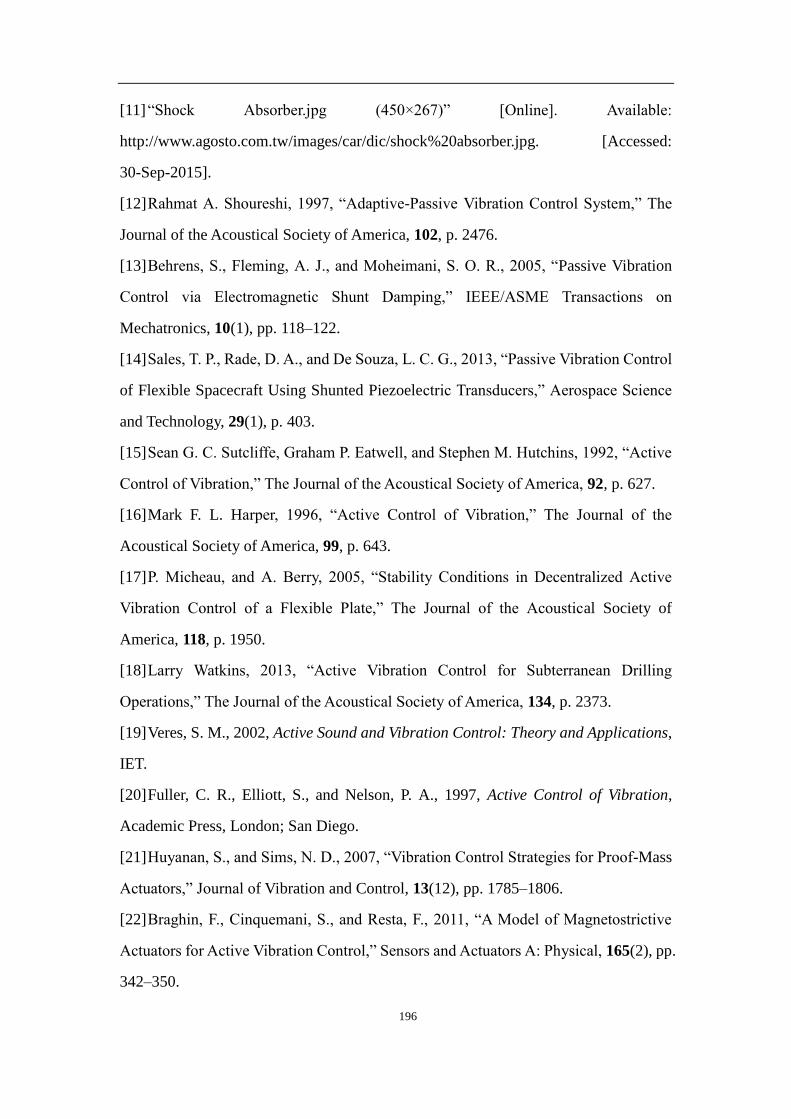
196
[11] “Shock Absorber.jpg (450×267)” [Online]. Available:
http://www.agosto.com.tw/images/car/dic/shock%20absorber.jpg. [Accessed:
30-Sep-2015].
[12] Rahmat A. Shoureshi, 1997, “Adaptive-Passive Vibration Control System,” The
Journal of the Acoustical Society of America, 102, p. 2476.
[13] Behrens, S., Fleming, A. J., and Moheimani, S. O. R., 2005, “Passive Vibration
Control via Electromagnetic Shunt Damping,” IEEE/ASME Transactions on
Mechatronics, 10(1), pp. 118–122.
[14] Sales, T. P., Rade, D. A., and De Souza, L. C. G., 2013, “Passive Vibration Control
of Flexible Spacecraft Using Shunted Piezoelectric Transducers,” Aerospace Science
and Technology, 29(1), p. 403.
[15] Sean G. C. Sutcliffe, Graham P. Eatwell, and Stephen M. Hutchins, 1992, “Active
Control of Vibration,” The Journal of the Acoustical Society of America, 92, p. 627.
[16] Mark F. L. Harper, 1996, “Active Control of Vibration,” The Journal of the
Acoustical Society of America, 99, p. 643.
[17] P. Micheau, and A. Berry, 2005, “Stability Conditions in Decentralized Active
Vibration Control of a Flexible Plate,” The Journal of the Acoustical Society of
America, 118, p. 1950.
[18] Larry Watkins, 2013, “Active Vibration Control for Subterranean Drilling
Operations,” The Journal of the Acoustical Society of America, 134, p. 2373.
[19] Veres, S. M., 2002, Active Sound and Vibration Control: Theory and Applications,
IET.
[20] Fuller, C. R., Elliott, S., and Nelson, P. A., 1997, Active Control of Vibration,
Academic Press, London; San Diego.
[21] Huyanan, S., and Sims, N. D., 2007, “Vibration Control Strategies for Proof-Mass
Actuators,” Journal of Vibration and Control, 13(12), pp. 1785–1806.
[22] Braghin, F., Cinquemani, S., and Resta, F., 2011, “A Model of Magnetostrictive
Actuators for Active Vibration Control,” Sensors and Actuators A: Physical, 165(2), pp.
342–350.

197
[23] Preumont, A., 2011, Vibration Control of Active Structures: An Introduction,
Springer, Berlin.
[24] Kimihiko Nakano, M. O., 2010, “Feasibility Study on Self-Powered Active
Vibration Control Using a Piezoelectric Actuator.”
[25] Liu, Y., Matsuhisa, H., and Utsuno, H., 2008, “Semi-Active Vibration Isolation
System with Variable Stiffness and Damping Control,” Journal Of Sound And
Vibration, 313(1–2), pp. 16–28.
[26] Caruso, G., Ben Mekki, O., and Bourquin, F., 2009, “Modeling and Experimental
Validation of a New Electromechanical Damping Device,” Journal of Vibroengineering,
11(4), p. 9p.
[27] Kasemi, B., Muthalif, A. G. A., Rashid, M. M., and Fathima, S., 2012, “Fuzzy-PID
Controller for Semi-Active Vibration Control Using Magnetorheological Fluid
Damper.”
[28] Ishida, Y., 2012, “Recent Development of the Passive Vibration Control Method,”
Mechanical Systems and Signal Processing, 29, pp. 2–18.
[29] Ming-Lai Lai, 1997, “Tuned Mass Damper,” The Journal of the Acoustical Society
of America, 102, p. 678.
[30] Weber, F., Boston, C., and Maslanka, M., 2011, “An Adaptive Tuned Mass Damper
Based on the Emulation of Positive and Negative Stiffness with an MR Damper,” Smart
Materials & Structures, 20(1).
[31] Michael E. McGuire, 2011, “Spare Tire Tuned Mass Damper,” The Journal of the
Acoustical Society of America, 130, p. 1083.
[32] Smith, M. C., 2002, “Synthesis of Mechanical Networks: The Inerter,” IEEE
Transactions on Automatic Control, 47(10), pp. 1648–1662.
[33] Rivin, E. I., 2003, Passive Vibration Isolation, ASME Press, New York.
[34] Wang, F.-C., and Wu, S.-Y., 2014, “Vibration Control of an Optical Table
Employing Mechatronic Inerter Networks,” Journal of Vibration and Control, 1, pp.
56–78.
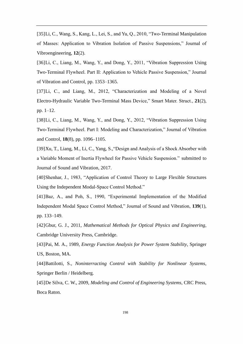
198
[35] Li, C., Wang, S., Kang, L., Lei, S., and Yu, Q., 2010, “Two-Terminal Manipulation
of Masses: Application to Vibration Isolation of Passive Suspensions,” Journal of
Vibroengineering, 12(2).
[36] Li, C., Liang, M., Wang, Y., and Dong, Y., 2011, “Vibration Suppression Using
Two-Terminal Flywheel. Part II: Application to Vehicle Passive Suspension,” Journal
of Vibration and Control, pp. 1353–1365.
[37] Li, C., and Liang, M., 2012, “Characterization and Modeling of a Novel
Electro-Hydraulic Variable Two-Terminal Mass Device,” Smart Mater. Struct., 21(2),
pp. 1–12.
[38] Li, C., Liang, M., Wang, Y., and Dong, Y., 2012, “Vibration Suppression Using
Two-Terminal Flywheel. Part I: Modeling and Characterization,” Journal of Vibration
and Control, 18(8), pp. 1096–1105.
[39] Xu, T., Liang, M., Li, C., Yang, S.,“Design and Analysis of a Shock Absorber with
a Variable Moment of Inertia Flywheel for Passive Vehicle Suspension.” submitted to
Journal of Sound and Vibration, 2017.
[40] Shenhar, J., 1983, “Application of Control Theory to Large Flexible Structures
Using the Independent Modal-Space Control Method.”
[41] Baz, A., and Poh, S., 1990, “Experimental Implementation of the Modified
Independent Modal Space Control Method,” Journal of Sound and Vibration, 139(1),
pp. 133–149.
[42] Gbur, G. J., 2011, Mathematical Methods for Optical Physics and Engineering,
Cambridge University Press, Cambridge.
[43] Pai, M. A., 1989, Energy Function Analysis for Power System Stability, Springer
US, Boston, MA.
[44] Battilotti, S., Noninterracting Control with Stability for Nonlinear Systems,
Springer Berlin / Heidelberg.
[45] De Silva, C. W., 2009, Modeling and Control of Engineering Systems, CRC Press,
Boca Raton.

199
[46] Bueno De Araujo, P., and Zanetta Jr., L. C., 2001, “Pole Placement Method Using
the System Matrix Transfer Function and Sparsity,” International Journal of Electrical
Power and Energy System, 23(3), pp. 173–178.
[47] Zubov, N., Mikrin, E., Misrikhanov, M. S., and Ryabchenko, V., 2013,
“Modification of the Exact Pole Placement Method and Its Application for the Control
of Spacecraft Motion,” Journal Of Computer And Systems Sciences International,
52(2), pp. 279–292.
[48] Dyer, P., 1970, Computation and Theory of Optimal Control, Elsevier.
[49] Speyer, J. L., 2010, Primer on Optimal Control Theory, Society for Industrial and
Applied Mathematics.
[50] Tiba, D., 1990, Optimal Control of Nonsmooth Distributed Parameter Systems.
[51] 1993, Optimal Control.
[52] Pavel, N. H., Corduneanu, C., and International Conference on Optimal Control of
Differential Equations : Athens, O., 1994, Optimal Control of Differential Equations,
MDekker, New York.
[53] Oborn, J., Bertilsson, H., and Rigdahl, M., 2001,
“Styrene-Ethylene/Butylene-Styrene Blends for Improved Constrained-Layer
Damping,” Journal Of Applied Polymer Science, 80(14), pp. 2865–2876.
[54] Liya Bochkareva, and Maksim Kireitseu, 2006, “Metal‐polymer‐ ceramic
Constrained Layer Damping System,” The Journal of the Acoustical Society of
America, 119, p. 3299.
[55] Cao, X., Zhang, Z., and Hua, H., 2011, “Free Vibration of Circular Cylindrical
Shell with Constrained Layer Damping,” Applied Mathematics and Mechanics, 32(4),
pp. 495–506.
[56] Xie, Z., Wong, P. K., and Lo, K. H., 2012, “Optimal Vibration Control of a
Rotating Plate with Self-Sensing Active Constrained Layer Damping.”
[57] Liang, Y.-J., and Wu, S.-L., 2013, “Optimal Vibration Control for Tracked Vehicle
Suspension Systems,” Mathematical Problems in Engineering, 2013.

200
[58] Lewis, F. L., 2014, Cooperative Control of Multi-Agent Systems : Optimal and
Adaptive Design Approaches, Springer, London.
[59] I. P. Priban, and W. F. Fincham, 1965, “Self-Adaptive Control and the Respiratory
System,” Nature, 208(5008), p. 339.
[60] Li, F., and Xie, J., 1998, “Practical Realization of a Self-Adaptive Feed-Forward
Control System for RF Gun Beam-Loading Compensation,” Nuclear Inst. and Methods
in Physics Research, A, 407(1), pp. 332–337.
[61] Qi, C., Pan, H., and Wang, Y., 2012, “Design and Realization of Two-Axis
Horizontal Stabilized Platform Based on Self-Correction Control Method.”
[62] Dones, I., Manenti, F., Preisig, H., and Buzzi-Ferraris, G., 2010, “Nonlinear Model
Predictive Control: A Self-Adaptive Approach,” Industrial & Engineering Chemistry
Research, 49(10), pp. 4782–4791.
[63] Valoor, M. T., Chandrashekhara, S., and Agarwal, S., 2001, “Self-Adaptive
Vibration Control of Smart Composite Beams Using Recurrent Neural Architecture,”
International Journal of Solids and Structures, 38(44–45), pp. 7857–7874.
[64] Hammond, P. H., Society of Instrument Technology, National Physical Laboratory,
and International Federation of Automatic Control, 1966, Theory of Self-Adaptive
Control Systems; Proceedings., New York, Plenum Press.
[65] Mackenroth, U., 2004, Robust Control Systems : Theory and Case Studies,
Springer, Berlin ; New York.
[66] Sun, W., Gao, H., and Yao, B., 2013, “Adaptive Robust Vibration Control of
Full-Car Active Suspensions With Electrohydraulic Actuators,” Ieee Transactions On
Control Systems Technology, 21(6), pp. 2417–2422.
[67] Nguyen, V., and Choi, S. B., 2011, “A Robust Vibration Control for a Multi-Active
Mount System Subjected to Broadband Excitation,” Smart Materials & Structures,
20(5).
[68] Ayyub, B. M., Guran, A., and Haldar, A., 1997, Uncertainty Modeling in Vibration,
Control and Fuzzy Analysis of Structural Systems, World Scientific, Singapore ; River
Edge, NJ.

201
[69] Li, D., and Xu, R., 2013, “Autonomous Decentralized Intelligent Vibration Control
for Large Split-Blanket Solar Arrays,” Science China Technological Sciences, 56(3),
pp. 703–712.
[70] Selected, peer reviewed papers from the I. C. on I. S. and V. C. (ISVC), 2011,
Intelligent Structure and Vibration Control : Selected, Peer Reviewed Papers from the
International Conference on Intelligent Structure and Vibration Control (ISVC) 2011,
January 14-16, 2011, Chongqing, China, Trans Tech Publications Ltd, Switzerland.
[71] Muradova, A. D., and Stavroulakis, G. E., 2013, “Fuzzy Vibration Control of a
Smart Plate,” International Journal of Computational Methods in Engineering Science
and Mechanics, 14(3), pp. 212–220.
[72] Gordon, T. J., Marsh, C., and Wu, Q. H., 1993, “Stochastic Optimal Control of
Active Vehicle Suspensions Using Learning Automata,” Proceedings of the Institution
of Mechanical Engineers. Part I, Journal of systems and control engineering, 207(3), pp.
143–152.
[73] Valavanis, K. P., 2009, Applications of Intelligent Control to Engineering Systems.
[74] Moretti, P. M., 2000, Modern Vibrations Primer, CRC Press, Boca Raton, Fla.
[75] Nwokah, O. D. I., and Hurmuzlu, Y., 2002, The Mechanical Systems Design
Handbook : Modeling, Measurement, and Control, CRC Press, Boca Raton, Fla.
[76] Preumont, A., 2008, Active Control of Structures.
[77] Yalla, S. K., Kareem, A., and Kantor, J. C., 2000, “Semi-Active Variable Damping
Liquid Column Dampers,” Proceedings of SPIE - The International Society for Optical
Engineering, 3988, pp. 75–83.
[78] Zhang, Y., 2001, “Semi-Active Control of Dynamically Excited Structures Using
Active Interaction Control.”
[79] Sahasrabudhe, S., 2002, “Semi-Active Control of Sliding Isolated Buildings and
Bridges with Variable Stiffness and Damping Systems.”
[80] Guglielmino, E., 2008, Semi-Active Suspension Control.
[81] Guglielmino, E., 2008, Semi-Active Suspension Control Improved Vehicle Ride and
Road Friendliness, Springer, London.

202
[82] Savaresi, S. M., 2010, Semi-Active Suspension Control Design for Vehicles,
Elsevier ; Kidlington, Oxford, UK; Burlington, Mass, Amsterdam ; Boston.
[83] Liu, H. (Professor of I. S., Gao, H., Li, P., and Institution of Engineering and
Technology, publisher, 2013, Handbook of Vehicle Suspension Control Systems, The
Institution of Engineering and Technology, ©2014, London.
[84] 2014, “Hydraulic Shock Absorber,” Mena Report.
[85] Shih, M. C., and Wang, T., 2008, “Active Control of Electro-Rheological Fluid
Embedded Pneumatic Vibration Isolator,” Integrated Computer-Aided Engineering,
15(3), pp. 267–276.
[86] Jiang, Z., and Christenson, R., 2012, “A Fully Dynamic Magneto-Rheological
Fluid Damper Model,” Smart Materials And Structures, 21(6).
[87] Suh, M. S., and Yeo, M. S., 1999, “Development of Semi-Active Suspension
Systems Using ER Fluids for the Wheeled Vehicle,” Journal Of Intelligent Material
Systems And Structures, 10(9), pp. 743–747.
[88] Dogruer, U., Gordaninejad, F., Evrensel, C. A., and Gordaninejad, F., 2003, “A
New Magneto-Rheological Fluid Damper for High-Mobility Multi-Purpose Wheeled
Vehicle (HMMWV).”
[89] Dogruer, U., Gordaninejad, F., Evrensel, C., Dogruer, U., Gordaninejad, F., and
Evrensel, C., 2004, “A Magneto-Rheological Fluid Damper for High-Mobility
Multi-Purpose Wheeled Vehicle (HMMWV).”
[90] Karakas, E. S., Gordaninejad, F., Evrensel, C. A., Yeo, M.-S., Liu, Y., Sahin, H.,
Karakas, E. S., Gordaninejad, F., Evrensel, C. A., Liu, Y., Sahin, H., and Yeo, M.-S.,
2004, “Control of a Quarter HMMWV Suspension System Using a
Magneto-Rheological Fluid Damper.”
[91] Mead, D. J., 1998, Passive Vibration Control, Wiley, Chichester ; New York.
[92] Krysinski, T., 2007, Mechanical Vibrations Active and Passive Control, ISTE,
London ; Newport Beach, CA.
[93] Rees, D. W. A., 2009, Mechanics of Optimal Structural Design : Minimum Weight
Structures, Chichester John Wiley & Sons, Ltd.
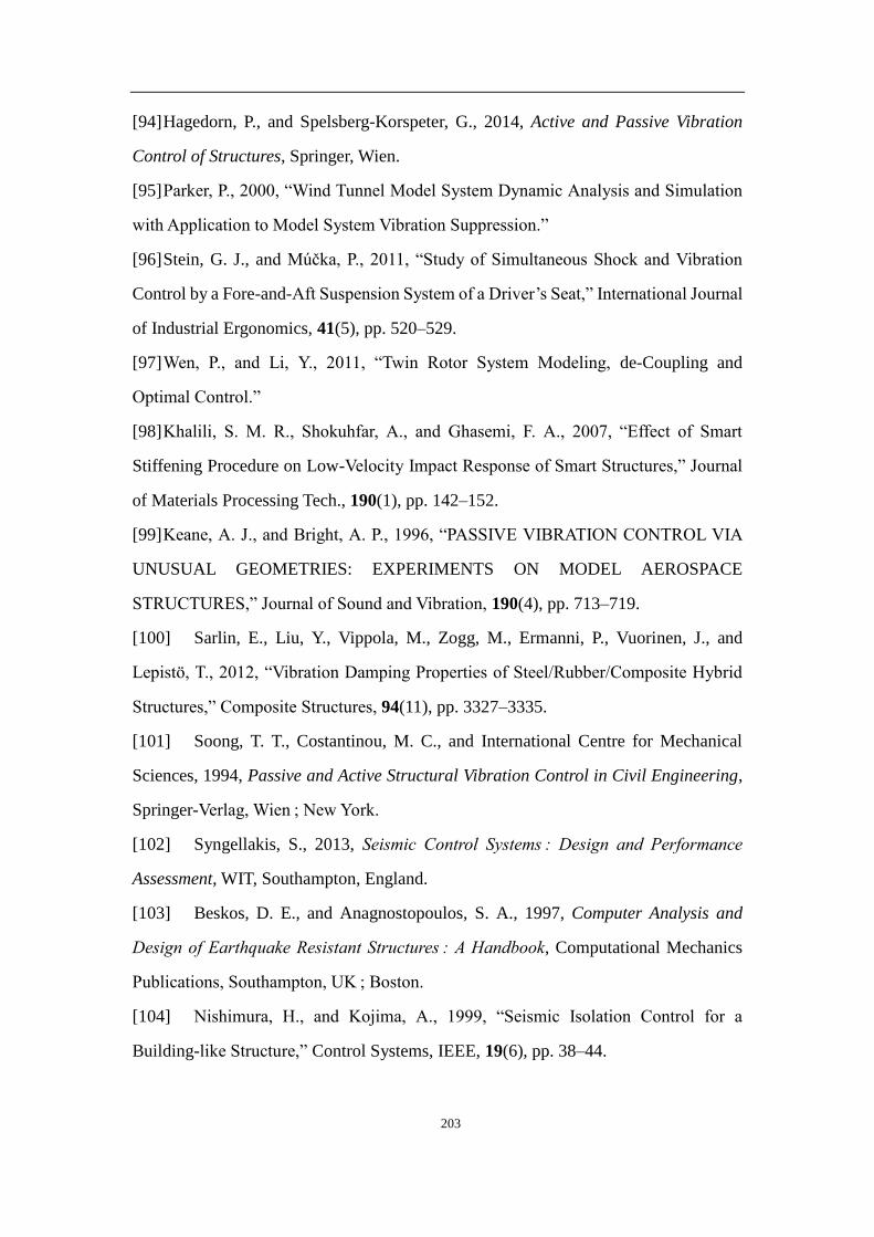
203
[94] Hagedorn, P., and Spelsberg-Korspeter, G., 2014, Active and Passive Vibration
Control of Structures, Springer, Wien.
[95] Parker, P., 2000, “Wind Tunnel Model System Dynamic Analysis and Simulation
with Application to Model System Vibration Suppression.”
[96] Stein, G. J., and Múčka, P., 2011, “Study of Simultaneous Shock and Vibration
Control by a Fore-and-Aft Suspension System of a Driver‟s Seat,” International Journal
of Industrial Ergonomics, 41(5), pp. 520–529.
[97] Wen, P., and Li, Y., 2011, “Twin Rotor System Modeling, de-Coupling and
Optimal Control.”
[98] Khalili, S. M. R., Shokuhfar, A., and Ghasemi, F. A., 2007, “Effect of Smart
Stiffening Procedure on Low-Velocity Impact Response of Smart Structures,” Journal
of Materials Processing Tech., 190(1), pp. 142–152.
[99] Keane, A. J., and Bright, A. P., 1996, “PASSIVE VIBRATION CONTROL VIA
UNUSUAL GEOMETRIES: EXPERIMENTS ON MODEL AEROSPACE
STRUCTURES,” Journal of Sound and Vibration, 190(4), pp. 713–719.
[100] Sarlin, E., Liu, Y., Vippola, M., Zogg, M., Ermanni, P., Vuorinen, J., and
Lepistö, T., 2012, “Vibration Damping Properties of Steel/Rubber/Composite Hybrid
Structures,” Composite Structures, 94(11), pp. 3327–3335.
[101] Soong, T. T., Costantinou, M. C., and International Centre for Mechanical
Sciences, 1994, Passive and Active Structural Vibration Control in Civil Engineering,
Springer-Verlag, Wien ; New York.
[102] Syngellakis, S., 2013, Seismic Control Systems : Design and Performance
Assessment, WIT, Southampton, England.
[103] Beskos, D. E., and Anagnostopoulos, S. A., 1997, Computer Analysis and
Design of Earthquake Resistant Structures : A Handbook, Computational Mechanics
Publications, Southampton, UK ; Boston.
[104] Nishimura, H., and Kojima, A., 1999, “Seismic Isolation Control for a
Building-like Structure,” Control Systems, IEEE, 19(6), pp. 38–44.
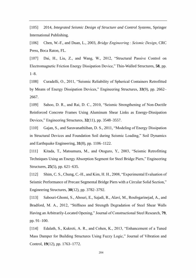
204
[105] 2014, Integrated Seismic Design of Structure and Control Systems, Springer
International Publishing.
[106] Chen, W.-F., and Duan, L., 2003, Bridge Engineering : Seismic Design, CRC
Press, Boca Raton, FL.
[107] Dai, H., Liu, Z., and Wang, W., 2012, “Structural Passive Control on
Electromagnetic Friction Energy Dissipation Device,” Thin-Walled Structures, 58, pp.
1–8.
[108] Curadelli, O., 2011, “Seismic Reliability of Spherical Containers Retrofitted
by Means of Energy Dissipation Devices,” Engineering Structures, 33(9), pp. 2662–
2667.
[109] Sahoo, D. R., and Rai, D. C., 2010, “Seismic Strengthening of Non-Ductile
Reinforced Concrete Frames Using Aluminum Shear Links as Energy-Dissipation
Devices,” Engineering Structures, 32(11), pp. 3548–3557.
[110] Gajan, S., and Saravanathiiban, D. S., 2011, “Modeling of Energy Dissipation
in Structural Devices and Foundation Soil during Seismic Loading,” Soil Dynamics
and Earthquake Engineering, 31(8), pp. 1106–1122.
[111] Kitada, T., Matsumura, M., and Otoguro, Y., 2003, “Seismic Retrofitting
Techniques Using an Energy Absorption Segment for Steel Bridge Piers,” Engineering
Structures, 25(5), pp. 621–635.
[112] Shim, C. S., Chung, C.-H., and Kim, H. H., 2008, “Experimental Evaluation of
Seismic Performance of Precast Segmental Bridge Piers with a Circular Solid Section,”
Engineering Structures, 30(12), pp. 3782–3792.
[113] Sabouri-Ghomi, S., Ahouri, E., Sajadi, R., Alavi, M., Roufegarinejad, A., and
Bradford, M. A., 2012, “Stiffness and Strength Degradation of Steel Shear Walls
Having an Arbitrarily-Located Opening,” Journal of Constructional Steel Research, 79,
pp. 91–100.
[114] Edalath, S., Kukreti, A. R., and Cohen, K., 2013, “Enhancement of a Tuned
Mass Damper for Building Structures Using Fuzzy Logic,” Journal of Vibration and
Control, 19(12), pp. 1763–1772.

205
[115] Novo, T., Varum, H., Teixeira-Dias, F., Rodrigues, H., Silva, M., Costa, A.,
and Guerreiro, L., 2014, “Tuned Liquid Dampers Simulation for Earthquake Response
Control of Buildings,” Bulletin of Earthquake Engineering, 12(2), pp. 1007–1024.
[116] Setareh, M., Ritchey, J. K., Baxter, A. J., and Murray, T. M., 2006, “Pendulum
Tuned Mass Dampers for Floor Vibration control.(Author Abstract),” Journal of
Performance of Constructed Facilities, 20(1), p. 64.
[117] Weng, F., and Mao, W., 2012, “Parameter-Dependent Vibration-Attenuation
Controller Design for Electro-Hydraulic Actuated Linear Structural Systems,”
Earthquake Engineering and Engineering Vibration, 11(1), pp. 73–82.
[118] Brebbia, C. A., 2005, Earthquake Resistant Engineering Structures V, WIT
Press, Southampton, UK ; Boston.
[119] Lin, C.-C., Lu, L.-Y., Lin, G.-L., and Yang, T.-W., 2010, “Vibration Control of
Seismic Structures Using Semi-Active Friction Multiple Tuned Mass Dampers,”
Engineering Structures, 32(10), pp. 3404–3417.
[120] Steinbuch, R., 2011, “Bionic Optimisation of the Earthquake Resistance of
High Buildings by Tuned Mass Dampers,” Journal of Bionic Engineering, 8(3), pp.
335–344.
[121] Ribeiro, E. A., Pereira, J. T., and Alberto Bavastri, C., 2015, “Passive
Vibration Control in Rotor Dynamics: Optimization of Composed Support Using
Viscoelastic Materials,” Journal of Sound and Vibration, 351, pp. 43–56.
[122] Bompos, D. A., and Nikolakopoulos, P. G., 2015, “Rotordynamic Analysis of
a Shaft Using Magnetorheological and Nanomagnetorheological Fluid Journal
Bearings,” Tribology Transactions, pp. 00–00.
[123] Sinha, A., 2010, Vibration of Mechanical Systems, Cambridge University
Press, Cambridge.
[124] Newland, D. E., 2006, Mechanical Vibration Analysis and Computation,
Dover Publications, Mineola, NY.
[125] A, T., 1971, “Vibrations and Their Dampers of Shaft Systems Supported by
Ball Bearings,” Lubrication, 16, pp. 1–8.

206
[126] Adams, M. L., 2010, Rotating Machinery Vibration from Analysis to
Troubleshooting, CRC Press/Taylor & Francis, Boca Raton Fla.
[127] Zhou, W. J., Yang, Y. C., Xing, G. K., and Wang, L. Q., 2013, “Numerical
Investigation of Nonlinear Vibration for Rotor-Seal System of Centrifugal Pump,” IOP
Conference Series: Materials Science and Engineering, 52(3), p. 5.
[128] Zhang, W., Yang, J., Gao, Q., and Li, J., 2014, “Reducing the Influence of
Partial Admission on Unstable Synchronous Vibration of Turbines by Bearing
Elevation Optimization,” Proceedings of the Institution of Mechanical Engineers, Part
C: Journal of Mechanical Engineering Science, 228(1), pp. 56–66.
[129] Ishida, Y., and Liu, J., 2010, “Elimination of Unstable Ranges of Rotors
Utilizing Discontinuous Spring Characteristics: An Asymmetrical Shaft System, an
Asymmetrical Rotor System, and a Rotor System With Liquid,” Journal Of Vibration
And Acoustics-Transactions Of The Asme, 132(1).
[130] Cai, K., Yin, H., Qin, Q., and Li, Y., 2014, “Self-Excited Oscillation of
Rotating Double-Walled Carbon Nanotubes,” Nano Letters, 14(5), pp. 2558–2562.
[131] Zhang, L., Li, X., Yao, Y., and Yang, L., 2010, “Study on Cascaded
Whole-Leaf Spring Oscillation Mechanism for Mould in Continuous Casting,”
Ironmaking & Steelmaking, 37(3), pp. 204–210.
[132] Tuplin, W. A., 1966, Torsional Vibration., Pitnam, London.
[133] Hidehiko Kuroda, 2007, “Torsional Vibration Measuring Instrument,” The
Journal of the Acoustical Society of America, 121, p. 1281.
[134] Inman, D. J., 2001, Engineering Vibration, Prentice Hall, Englewood Cliffs,
NJ.
[135] Walker, D. N., 2004, Torsional Vibration of Turbomachinery, McGraw-Hill,
New York.
[136] Janusz Walkowc, 1997, “Active Torsional Vibration Damper,” The Journal of
the Acoustical Society of America, 102, p. 3248.
[137] Reimpell, J., 2001, The Automotive Chassis Engineering Principles : Chassis
and Vehicle Overall, Wheel Suspensions and Types of Drive, Axle Kinematics and

207
Elastokinematics, Steering, Springing, Tyres, Construction and Calculations Advice.,
Butterworth Heinemann, Oxford.
[138] Sandin, P. E., 2003, Robot Mechanisms and Mechanical Devices Illustrated,
McGraw-Hill, New York.
[139] Chen, Y. W., 2014, Structural Genomics : General Applications, Humana
Press, New York.
[140] Qiu, J. S., and Meng, J., 2011, “Nonlinear Finite Element Analysis and
Experimental Study of Leaf Spring Suspension.”
[141] N. Lavanya, and P. Sampath Rao, 2014, “Design and Analysis of A Suspension
Coil Spring For Automotive Vehicle,” International Journal of Engineering Research
and Applications, 4(9), p. 151.
[142] 2006, “Design Engineering - Air Spring Suspension: Air of Intelligence,” The
Engineer, pp. 47–48.
[143] Matschinsky, W., 2000, Road Vehicle Suspensions, Professional Engineering
Pub, London, UK.
[144] Le, K. C., and Pieper, A., 2014, “Damping of Roll Vibrations of Vehicle
Suspension,” Vehicle System Dynamics, pp. 1–18.
[145] Society of Automotive Engineers, and SAE World Congress : Detroit, M. ),
2007, Reliability and Robust Design in Automotive Engineering, 2007., Society of
Automotive Engineers, Warrendale, Pa.
[146] Blundell, M., 2004, Multibody Systems Approach to Vehicle Dynamics,
Burlington Butterworth-Heinemann.
[147] Arikere, A., Saravana Kumar, G., and Bandyopadhyay, S., 2010,
“Optimisation of Double Wishbone Suspension System Using Multi-Objective Genetic
Algorithm.”
[148] Uchida, T., and Mcphee, J., 2012, “Driving Simulator with Double-Wishbone
Suspension Using Efficient Block-Triangularized Kinematic Equations,” Multibody
System Dynamics, 28(4), pp. 331–347.

208
[149] Cheng, X., and Lin, Y., 2014, “Multiobjective Robust Design of the Double
Wishbone Suspension System Based on Particle Swarm Optimization,” Scientific
World Journal.
[150] Blanco, J. C., and Munoz, L. E., 2014, “Multi-Objective Optimization of the
Geometry of a Double Wishbone Suspension System,” Vibroengineering Procedia, 3, p.
70.
[151] Balike, K., Rakheja, S., and Stiharu, I., 2011, “Development of
Kineto-Dynamic Quarter-Car Model for Synthesis of a Double Wishbone Suspension,”
Vehicle System Dynamics, 49(1–2), pp. 107–128.
[152] Shi, C. H., Kang, S. H., Li, C. H., Huang, L., Shi, C. H., Zhang, X. Z., and Hu,
J. Z., 2014, “Design and Analysis of Double Wishbone Suspension Module with
Wheel-Track Variant Wheels.”
[153] Dhir, A., and Sankar, S., 1995, “Dynamics of off-Road Tracked Vehicles
Equipped with Trailing Arm Suspension,” Proceedings Of The Institution Of
Mechanical Engineers Part D-Journal Of Au, 209(3), pp. 195–215.
[154] Wang, W., Li, Y., Zhang, S., and Wang, B., 2014, “Research on the Ride
Comfort of Electric Drive System Based on Double Trailing Arm Suspension.”
[155] Zhao, J.-S., Li, L., Chen, L., and Zhang, Y., 2010, “The Concept Design and
Dynamics Analysis of a Novel Vehicle Suspension Mechanism with Invariable
Orientation Parameters,” Vehicle System Dynamics, 48(12), pp. 1495–1510.
[156] Kang, H. Y., and Suh, C. H., 1994, “Synthesis and Analysis
Spherical-Cylindrical (SC) Link in the McPherson Strut Suspension Mechanism,”
Journal of Mechanical Design, 116(2), p. 599.
[157] Habibi, H., Shirazi, K. H., and Shishesaz, M., 2008, “Roll Steer Minimization
of McPherson-Strut Suspension System Using Genetic Algorithm Method,”
Mechanism and Machine Theory, 43(1), pp. 57–67.
[158] Kang, D.-O., Heo, S.-J., and Kim, M.-S., 2010, “Robust Design Optimization
of the McPherson Suspension System with Consideration of a Bush Compliance

209
Uncertainty,” Proceedings of the Institution of Mechanical Engineers, Part D: Journal
of Automobile Engineering, 224(6), pp. 705–716.
[159] Anderson, B. D. O., 1973, Network Analysis and Synthesis: A Modern Systems
Theory Approach, Englewood Cliffs, NJ: Prentice-Hall.
[160] Storer, J. E., 1957, Passive Network Synthesis. --, McGraw-Hill, New York.
[161] Chen, W.-K., and ScienceDirect, 2005, The Electrical Engineering Handbook,
Elsevier Academic Press, Boston.
[162] Ulrich, R. K., and Schaper, L. W., 2003, Integrated Passive Component
Technology, IEEE Press ; Hoboken, NJ, Piscataway, NJ.
[163] Uhlig, S., 2007, Passive and Active Network Measurement.
[164] Zobrist, G. W., 1965, Digital Computer Analysis of Passive Networks Using
Topological Formulas \, Deptof Electrical Engineering, University of Missouri,
Columbia.
[165] Anderson, B., and Kailath, T., 1979, “Passive Network Synthesis via Dual
Spectral Factorization,” Circuits and Systems, IEEE Transactions on, 26(10), pp. 866–
873.
[166] Guillemin, E. A., 1957, Synthesis of Passive Networks; Theory and Methods
Appropriate to the Realization and Approximation Problems., New York, Wiley 1957.
[167] Smith, M. C., and Walker, G., 2000, “Performance Limitations and Constraints
for Active and Passive Suspensions: A Mechanical Multi-Port Approach,” Vehicle
System Dynamics, 33(3), pp. 137–168.
[168] Hu, Y., and Chen, M. Z. Q., 2015, “Performance Evaluation for Inerter-Based
Dynamic Vibration Absorbers,” International Journal of Mechanical Sciences.
[169] Wang, F., Hong, M., and Lin, T. C., 2011, “Designing and Testing a Hydraulic
Inerter,” Proceedings Of The Institution Of Mechanical Engineers Part C-Journal Of
Me, 225(C1), pp. 66–72.
[170] Lazar, I. F., Neild, S. A., and Wagg, D. J., 2014, “Using an Inerter‐based
Device for Structural Vibration Suppression,” Earthquake Engineering & Structural
Dynamics, 43(8), pp. 1129–1147.

210
[171] Smith, M. C., 2002, “Synthesis of Mechanical Networks: The Inerter,” Ieee
Transactions On Automatic Control, 47(10), pp. 1648–1662.
[172] Chen, M. Z. Q., Hu, Y., Li, C., and Chen, G., 2015, “Performance Benefits of
Using Inerter in Semiactive Suspensions,” Control Systems Technology, IEEE
Transactions on, 23(4), pp. 1571–1577.
[173] Li, C., Liang, M., Wang, Y., and Dong, Y., 2012, “Vibration Suppression Using
Two-Terminal Flywheel. Part I: Modeling and Characterization,” Journal Of Vibration
And Control, 18(8), pp. 1096–1105.
[174] Anderson, T. J., Anderson, M. J., Hocut, C., Zornik, W., and Blotter, J. D.,
2000, “Passive Vibration Suppression Using Nonlinear Electromechanical Coupling,”
The Journal of the Acoustical Society of America, 108(5), pp. 2478–2478.
[175] Guyomar, D., and Badel, A., 2006, “Nonlinear Semi-Passive Multimodal
Vibration Damping: An Efficient Probabilistic Approach,” Journal of Sound and
Vibration, 294(1), pp. 249–268.
[176] Peng, Z., Lang, Z., and Meng, G., 2012, “Evaluation of Transmissibility for a
Class of Nonlinear Passive Vibration Isolators,” Frontiers of Mechanical Engineering,
7(4), pp. 401–409.
[177] Nordin, M., Galic‟, J., and Gutman, P.-O., 1997, “New Models for Backlash
and Gear Play,” Int. J. Adapt. Control Signal Process., 11(1), pp. 49–63.
[178] Wang, X., ed., 2010, Vehicle Noise and Vibration Refinement, Woodhead
Publishing, Boca Raton, Fla.
[179] Sun, X., Chen, L., Wang, S., Zhang, X., and Yang, X., 2016, “Performance
Investigation of Vehicle Suspension System with Nonlinear Ball-Screw Inerter,”
International Journal of Automotive Technology, 17(3), pp. 399–408.
[180] Rath, J. J., Veluvolu, K. C., and Defoort, M., 2014, “Adaptive Super-Twisting
Observer for Estimation of Random Road Excitation Profile in Automotive Suspension
Systems,” TheScientificWorldJournal, 2014, p. 203416.

211
[181] Čorić, M., Deur, J., Xu, L., Tseng, H. E., and Hrovat, D., 2016, “Optimisation
of Active Suspension Control Inputs for Improved Vehicle Ride Performance,” Vehicle
System Dynamics, 54(7), pp. 1004–1030.
[182] Devdutt, M., and Aggarwal, M., 2015, “Fuzzy Control of Passenger Ride
Performance Using MR Shock Absorber Suspension in Quarter Car Model,”
International Journal of Dynamics and Control, 3(4), pp. 463–469.
[183] Lee, H.-G., Sung, K.-G., Choi, S.-B., Park, M.-K., and Park, M.-K., 2011,
“Performance Evaluation of a Quarter-Vehicle MR Suspension System with Different
Tire Pressure,” International Journal of Precision Engineering and Manufacturing,
12(2), pp. 203–210.
[184] Nguyen, L., Hong, K.-S., and Park, S., 2010, “Road-Frequency Adaptive
Control for Semi-Active Suspension Systems,” International Journal of Control,
Automation and Systems, 8(5), pp. 1029–1038.
[185] Naraghi, M., 1996, Dynamics and Control of Fast Automated Guided Vehicles
for High Load Applications., 1996.
[186] Jae-Hoon Lee, Changwan Han, Dongsu Ahn, Jin Kyoo Lee, Sang-Hu Park,
and Seonghun Park, 2013, “Design and Performance Evaluation of a Rotary
Magnetorheological Damper for Unmanned Vehicle Suspension Systems,” The
Scientific World Journal, 2013.
[187] Zhu, J.-Y., 2009, “Empirical Analysis of the Effect of Rural Education on
Income Distribution of Rural Labor Force - A Case of Yongchuan District, Chongqing,”
Asian Agricultural Research, 1.
[188] Kang, L., and Peng, F., 2013, “Cost Competitiveness Comparisons and
Convergence in China,” National Institute Economic Review, (223), p. 49.
[189] García-Saldaña, J. D., and Gasull, A., 2015, “The Period Function and the
Harmonic Balance Method,” Bulletin des sciences mathématiques, 139(1), pp. 33–60.
[190] Razzak, M. A., 2016, “A Simple Harmonic Balance Method for Solving
Strongly Nonlinear Oscillators,” Journal of the Association of Arab Universities for
Basic and Applied Sciences, 21, pp. 68–76.
212
[191] Mohammadian, M., and Shariati, M., 2017, “Approximate Analytical
Solutions to a Conservative Oscillator Using Global Residue Harmonic Balance
Method,” Chinese Journal of Physics, 55(1), pp. 47–58.
[192] Weisheit, K., and Marburg, S., 2016, “Calculation of the Response of a
Periodically Excited Beam with Frictional Contact Using Harmonic Balance Method,”
Procedia IUTAM, 19, pp. 282–288.
[193] Shen, Y.-J., Wen, S.-F., Li, X.-H., Yang, S.-P., and Xing, H.-J., 2016,
“Dynamical Analysis of Fractional-Order Nonlinear Oscillator by Incremental
Harmonic Balance Method,” Nonlinear Dynamics, 85(3), pp. 1457–1467.
[194] Molla, M. H. U., Razzak, M. A., and Alam, M. S., 2016, “Harmonic Balance
Method for Solving a Large-Amplitude Oscillation of a Conservative System with
Inertia and Static Non-Linearity,” Results in Physics, 6, pp. 238–242.
[195] Liu, J. K., Chen, F. X., and Chen, Y. M., 2012, “Bifurcation Analysis of
Aeroelastic Systems with Hysteresis by Incremental Harmonic Balance Method,”
Applied Mathematics and Computation, 219(5), pp. 2398–2411.
[196] Chen, Y. M., Liu, J. K., and Meng, G., 2011, “Incremental Harmonic Balance
Method for Nonlinear Flutter of an Airfoil with Uncertain-but-Bounded Parameters,”
Applied Mathematical Modelling.
[197] Celik, M., Atalar, A., and Tan, M. A., 1996, “A New Method for the
Steady-State Analysis of Periodically Excited Nonlinear Circuits,” Circuits and
Systems I: Fundamental Theory and Applications, IEEE Transactions on, 43(12), pp.
964–972.

213
Appendix A – Signals used in Model Validation
Table of part experimental data for section 4.1
Signal type Frequency Amplitude Recording
length
purpose
1 Triangular 0.1Hz 0.05m 100 seconds Identification
2 Triangular 0.1Hz 0.1m 100 seconds Identification
3 Triangular 0.2Hz 0.05m 50 seconds Identification
4 Triangular 0.2Hz 0.1m 50 seconds Identification
5 Triangular 0.5Hz 0.05m 20 seconds Identification
6 Triangular 0.5Hz 0.1m 20 seconds Validation
7 Triangular 0.5Hz 0.15m 20seconds Identification
8 Triangular 1Hz 0.05m 10 seconds Identification
9 Triangular 1Hz 0.1m 10 seconds Validation
10 Triangular 1Hz 0.15m 10 seconds Identification
11 Sinusoidal 0.1Hz 0.01m 100 seconds Validation
12 Sinusoidal 0.1Hz 0.02m 100 seconds Identification
13 Sinusoidal 0.1Hz 0.03m 100 seconds Validation
14 Sinusoidal 0.1Hz 0.05m 100 seconds Validation
15 Sinusoidal 0.1Hz 0.08m 100 seconds Validation
16 Sinusoidal 0.1Hz 0.10m 100 seconds Identification
17 Sinusoidal 0.1Hz 0.12m 100 seconds Validation
18 Sinusoidal 0.1Hz 0.15m 100 seconds Identification
19 Sinusoidal 0.2Hz 0.01m 50 seconds Validation
20 Sinusoidal 0.2Hz 0.02m 50 seconds Identification
21 Sinusoidal 0.2Hz 0.03m 50 seconds Validation
22 Sinusoidal 0.2Hz 0.05m 50 seconds Identification
23 Sinusoidal 0.2Hz 0.08m 50 seconds Validation
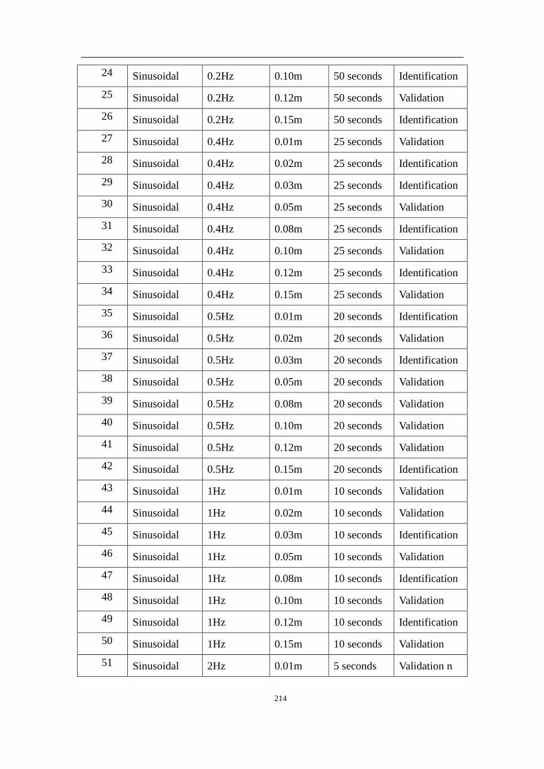
214
24 Sinusoidal 0.2Hz 0.10m 50 seconds Identification
25 Sinusoidal 0.2Hz 0.12m 50 seconds Validation
26 Sinusoidal 0.2Hz 0.15m 50 seconds Identification
27 Sinusoidal 0.4Hz 0.01m 25 seconds Validation
28 Sinusoidal 0.4Hz 0.02m 25 seconds Identification
29 Sinusoidal 0.4Hz 0.03m 25 seconds Identification
30 Sinusoidal 0.4Hz 0.05m 25 seconds Validation
31 Sinusoidal 0.4Hz 0.08m 25 seconds Identification
32 Sinusoidal 0.4Hz 0.10m 25 seconds Validation
33 Sinusoidal 0.4Hz 0.12m 25 seconds Identification
34 Sinusoidal 0.4Hz 0.15m 25 seconds Validation
35 Sinusoidal 0.5Hz 0.01m 20 seconds Identification
36 Sinusoidal 0.5Hz 0.02m 20 seconds Validation
37 Sinusoidal 0.5Hz 0.03m 20 seconds Identification
38 Sinusoidal 0.5Hz 0.05m 20 seconds Validation
39 Sinusoidal 0.5Hz 0.08m 20 seconds Validation
40 Sinusoidal 0.5Hz 0.10m 20 seconds Validation
41 Sinusoidal 0.5Hz 0.12m 20 seconds Validation
42 Sinusoidal 0.5Hz 0.15m 20 seconds Identification
43 Sinusoidal 1Hz 0.01m 10 seconds Validation
44 Sinusoidal 1Hz 0.02m 10 seconds Validation
45 Sinusoidal 1Hz 0.03m 10 seconds Identification
46 Sinusoidal 1Hz 0.05m 10 seconds Validation
47 Sinusoidal 1Hz 0.08m 10 seconds Identification
48 Sinusoidal 1Hz 0.10m 10 seconds Validation
49 Sinusoidal 1Hz 0.12m 10 seconds Identification
50 Sinusoidal 1Hz 0.15m 10 seconds Validation
51 Sinusoidal 2Hz 0.01m 5 seconds Validation n

215
52 Sinusoidal 2Hz 0.02m 5 seconds Validation
53 Sinusoidal 2Hz 0.03m 5 seconds Identification
54 Sinusoidal 2Hz 0.05m 5 seconds Validation
55 Sinusoidal 2Hz 0.08m 5 seconds Identification
56 Sinusoidal 2Hz 0.10m 5 seconds Validation
57 Sinusoidal 2Hz 0.12m 5 seconds Identification
58 Sinusoidal 2Hz 0.15m 5 seconds Validation
59 Sinusoidal 5Hz 0.01m 2 seconds Validation
60 Sinusoidal 5Hz 0.02m 2 seconds Identification
61 Sinusoidal 5Hz 0.03m 2 seconds Identification
62 Sinusoidal 5Hz 0.05m 2 seconds Validation
63 Sinusoidal 5Hz 0.08m 2 seconds Validation
64 Sinusoidal 10Hz 0.01m 1 seconds Validation
65 Sinusoidal 10Hz 0.02m 1 seconds Identification
66 Sinusoidal 10Hz 0.03m 1 seconds Validation
67 Sinusoidal 10Hz 0.05m 1 seconds Identification
68 Sinusoidal 10Hz 0.08m 1 seconds Validation
Table of part experimental data for section 4.2 and section 4.3
Signal type Frequency Amplitude Recording
length
purpose
1 Sinusoidal 0.1Hz 0.01m 100 seconds Validation
2 Sinusoidal 0.1Hz 0.02m 100 seconds Identification
3 Sinusoidal 0.1Hz 0.03m 100 seconds Validation
4 Sinusoidal 0.1Hz 0.05m 100 seconds Validation
5 Sinusoidal 0.1Hz 0.08m 100 seconds Validation
6 Sinusoidal 0.1Hz 0.10m 100 seconds Identification

216
7 Sinusoidal 0.1Hz 0.12m 100 seconds Validation
8 Sinusoidal 0.1Hz 0.15m 100 seconds Identification
9 Sinusoidal 0.1Hz 0.18m 100 seconds Validation
10 Sinusoidal 0.1Hz 0.20m 100 seconds Validation
11 Sinusoidal 0.2Hz 0.01m 50 seconds Validation
12 Sinusoidal 0.2Hz 0.02m 50 seconds Identification
13 Sinusoidal 0.2Hz 0.03m 50 seconds Validation
14 Sinusoidal 0.2Hz 0.05m 50 seconds Identification
15 Sinusoidal 0.2Hz 0.08m 50 seconds Validation
16 Sinusoidal 0.2Hz 0.10m 50 seconds Identification
17 Sinusoidal 0.2Hz 0.12m 50 seconds Validation
18 Sinusoidal 0.2Hz 0.15m 50 seconds Identification
19 Sinusoidal 0.2Hz 0.18m 50 seconds Validation
20 Sinusoidal 0.2Hz 0.20m 50 seconds Validation
21 Sinusoidal 0.4Hz 0.01m 25 seconds Validation
22 Sinusoidal 0.4Hz 0.02m 25 seconds Identification
23 Sinusoidal 0.4Hz 0.03m 25 seconds Identification
24 Sinusoidal 0.4Hz 0.05m 25 seconds Validation
25 Sinusoidal 0.4Hz 0.08m 25 seconds Identification
26 Sinusoidal 0.4Hz 0.10m 25 seconds Validation
27 Sinusoidal 0.4Hz 0.12m 25 seconds Identification
28 Sinusoidal 0.4Hz 0.15m 25 seconds Validation
29 Sinusoidal 0.4Hz 0.18m 25 seconds Validation
30 Sinusoidal 0.4Hz 0.20m 25 seconds Validation
31 Sinusoidal 0.5Hz 0.01m 20 seconds Identification
32 Sinusoidal 0.5Hz 0.02m 20 seconds Validation
33 Sinusoidal 0.5Hz 0.03m 20 seconds Identification
34 Sinusoidal 0.5Hz 0.05m 20 seconds Validation

217
35 Sinusoidal 0.5Hz 0.08m 20 seconds Validation
36 Sinusoidal 0.5Hz 0.10m 20 seconds Validation
37 Sinusoidal 0.5Hz 0.12m 20 seconds Validation
38 Sinusoidal 0.5Hz 0.15m 20 seconds Identification
39 Sinusoidal 0.5Hz 0.18m 20 seconds Validation
40 Sinusoidal 0.5Hz 0.20m 20 seconds Validation
41 Sinusoidal 1Hz 0.01m 10 seconds Validation
42 Sinusoidal 1Hz 0.02m 10 seconds Validation
43 Sinusoidal 1Hz 0.03m 10 seconds Identification
44 Sinusoidal 1Hz 0.05m 10 seconds Validation
45 Sinusoidal 1Hz 0.08m 10 seconds Identification
46 Sinusoidal 1Hz 0.10m 10 seconds Validation
47 Sinusoidal 1Hz 0.12m 10 seconds Identification
48 Sinusoidal 1Hz 0.15m 10 seconds Validation
49 Sinusoidal 1Hz 0.18m 10 seconds Validation
50 Sinusoidal 1Hz 0.20m 10 seconds Validation
51 Sinusoidal 2Hz 0.01m 5 seconds Validation n
52 Sinusoidal 2Hz 0.02m 5 seconds Validation
53 Sinusoidal 2Hz 0.03m 5 seconds Identification
54 Sinusoidal 2Hz 0.05m 5 seconds Validation
55 Sinusoidal 2Hz 0.08m 5 seconds Identification
56 Sinusoidal 2Hz 0.10m 5 seconds Validation
57 Sinusoidal 2Hz 0.12m 5 seconds Identification
58 Sinusoidal 2Hz 0.15m 5 seconds Validation
59 Sinusoidal 5Hz 0.01m 2 seconds Validation
60 Sinusoidal 5Hz 0.02m 2 seconds Identification
61 Sinusoidal 5Hz 0.03m 2 seconds Identification
62 Sinusoidal 5Hz 0.05m 2 seconds Validation

218
63 Sinusoidal 5Hz 0.08m 2 seconds Validation
64 Sinusoidal 5Hz 0.1m 2 seconds Validation
65 Sinusoidal 5Hz 0.12m 2 seconds Validation
66 Sinusoidal 5Hz 0.15m 2 seconds Validation
67 Sinusoidal 10Hz 0.01m 1 seconds Validation
68 Sinusoidal 10Hz 0.02m 1 seconds Identification
69 Sinusoidal 10Hz 0.03m 1 seconds Validation
70 Sinusoidal 10Hz 0.05m 1 seconds Identification
71 Sinusoidal 10Hz 0.12m 1 seconds Validation
72 Sinusoidal 10Hz 0.15m 1 seconds Validation

219
Appendix B - Code
Code of simulation:
t = cell(size(Freqs));
Resp = t;
Ft = t;
RespAmp = Freqs;
tSeg = zeros(size(t));
StartPnt = [];
N = length(nCycles);
t1 = cell(N,1);
Resp1 = t1;
Ft1 = t1;
for i = 1:N
ExParas.A = Amps(i); ExParas.Omega = 2 * pi * Freqs(i);
SysParas = fnUpdateSys(ExParas,SysParas,BWParas);
if ~isempty(StartPnt)
StartPnt(1) = StartPnt(1) / SysParas.L;
StartPnt(2) = SysParas.T / SysParas.L * StartPnt(2);
end
[~,f0] = fnExcite(SysParas,[]);
[t{i},Resp{i}] =
fnNumSim(SysParas,BWParas,fnExcite,f0,nCycles(i),StartPnt);
Ft{i} = fnExcite(SysParas,t{i});
[t{i},Resp{i}] = fnTransResult(t{i},Resp{i},SysParas);
[~,Ft{i}] = fnTransResult(t{i},Ft{i},SysParas);
RespAmp(i) = GetAmp(t{i},Resp{i}(:,1) + Ft{i},Freqs(i),false);
if i > 1
t1{i} = t1{i - 1}(end) + t{i}(2:end);
Resp1{i} = Resp{i}(2:end,1);
Ft1{i} = Ft{i}(2:end);
tSeg(i) = t1{i - 1}(end);
else
t1(i) = t(i);
Resp1{i} = Resp{i}(:,1);
Ft1{i} = Ft{i};
tSeg(i) = 0;
end
if ~isempty(hFigs)
if i > idxTurningPnt
bSweepUp = false;

220
else
bSweepUp = true;
end
UpdatePlot(t1{i},Ft1{i},Resp1{i},Freqs(i),hFigs,bSweepUp,2);
end
StartPnt = [Resp{i}(end,:)]';
end
for i = 1:N
end
t1 = cell2mat(t1);
Resp1 = cell2mat(Resp1);
Ft1 = cell2mat(Ft1);
end
function Amp = GetAmp(t,x,f0,bIncludeDC)
T = 2 / f0;
tStart = t(end) - T;
xStart = interp1(t,x,tStart,'pchip');
idx = find(t > tStart,1);
tAmp = [tStart;t(idx:end)];
Resp = [xStart;x(idx:end)];
DC = mean(Resp);
Amp = (max(Resp) - min(Resp)) / 2;
if bIncludeDC
Amp = Amp + DC;
end
end
function UpdatePlot(t,xg,x,f0,hFigs,bSweepUp,nPhaseCyclesCnt)
hFigx = []; hFigPhase = [];
if ~isempty(hFigs)
hFigx = hFigs(1);
if length(hFigs) == 2
hFigPhase = hFigs(2);
end
end
if bSweepUp
szStyle = 'y';
else
szStyle = 'g';
end
if ~isempty(hFigx)
figure(hFigx);
plot(t,x,szStyle);

221
plot(t,xg,'c--');
tmp = axis;
plot([t(1),t(1)],[tmp(3),tmp(4)],'r--');
end
if ~isempty(hFigPhase)
figure(hFigPhase);
tSpan = nPhaseCyclesCnt / f0;
idxStart = find(t <= t(end) - tSpan,1,'last');
plot(xg(idxStart:end),xg(idxStart:end) +
x(idxStart:end),szStyle);
end
end
function dz=fQCI(t,z)%quarter car impulse input
%z(1)=x3, z(2)=x3', z(3)=x2,
z(4)=x2',z(5)=x3e,z(6)=x3e',z(7)=x2e,z(8)=x2e',
mt=30;
m=320;
ct=700;
c=7000;
kt=100000;
k=80000;
dz=zeros(8,1);
t1=0;
t2=0.001;
dz(1)=z(2);
dz(2)=-k/m*(z(1)-z(3))-c/m*(z(2)-z(3));
dz(3)=z(4);
dz(4)=-kt/mt*(z(3)-(stepfun(t,t1)-stepfun(t,t2)))-ct/mt*z(4)+k/mt*(z(
1)-z(3))+c/mt*(z(2)-z(3));
dz(5)=z(6);
me=(0.000883+0.14*(2.025/(90-32368*(dz(6)-dz(8)).^2)).^2)*924797;
dz(6)=me/m*(dz(6)-dz(8))-k/m*(z(5)-z(7))-c/m*(z(6)-z(8));
dz(7)=z(8);
dz(8)=-me/mt*(dz(6)-dz(8))-kt/mt*(z(7)-(stepfun(t,t1)-stepfun(t,t2)))
-ct/mt*z(8)+k/mt*(z(5)-z(7))-c/mt*(z(6)-z(8));
end
function dz=fQCs(t,z)%quarter car sinusoidal input
%z(1)=x3, z(2)=x3', z(3)=x2,
z(4)=x2',z(5)=x3e,z(6)=x3e',z(7)=x2e,z(8)=x2e',
mt=30;
m=320;
222
ct=700;
c=7000;
kt=100000;
k=80000;
Ip=10*sin(2*t);
Ip1=20*cos(2*t);
dz=zeros(8,1);
dz(1)=z(2);
dz(2)=-k/m*(z(1)-z(3))-c/m*(z(2)-z(3));
dz(3)=z(4);
dz(4)=-kt/mt*(z(3)-Ip)-ct/mt*(z(4)-Ip1)+k/mt*(z(1)-z(3))+c/mt*(z(2)-z
(3));
dz(5)=z(6);
me=(0.000883+0.14*(2.025/(90-32368*(dz(6)-dz(8)).^2)).^2)*924797;
dz(6)=me/m*(dz(6)-dz(8))-k/m*(z(5)-z(7))-c/m*(z(6)-z(8));
dz(7)=z(8);
dz(8)=-me/mt*(dz(6)-dz(8))-kt/mt*(z(7)-Ip)-ct/mt*(z(8)-Ip1)+k/mt*(z(5
)-z(7))-c/mt*(z(6)-z(8));
end
function dz=fQCZ(t,z)%quarter car zero inout
%z(1)=x3, z(2)=x3', z(3)=x2,
z(4)=x2',z(5)=x3e,z(6)=x3e',z(7)=x2e,z(8)=x2e',
mt=30;
m=320;
ct=700;
c=7000;
kt=100000;
k=80000;
dz=zeros(8,1);
dz(1)=z(2);
dz(2)=-k/m*(z(1)-z(3))-c/m*(z(2)-z(3));
dz(3)=z(4);
dz(4)=-kt/mt*z(3)-ct/mt*z(4)+k/mt*(z(1)-z(3))+c/mt*(z(2)-z(3));
dz(5)=z(6);
me=(0.000883+0.14*(2.025/(90-32368*(dz(6)-dz(8)).^2)).^2)*924797;
dz(6)=me/m*(dz(6)-dz(8))-k/m*(z(5)-z(7))-c/m*(z(6)-z(8));
dz(7)=z(8);
dz(8)=-me/mt*(dz(6)-dz(8))-kt/mt*z(7)-ct/mt*z(8)+k/mt*(z(5)-z(7))-c/m
t*(z(6)-z(8));
end
x=[0 0.15 0.23 0.25 ];

223
y=[0 0.64 1.12 1 ];
values = spcrv([[x(1) x x(end)];[y(1) y y(end)]],3);
plot(values(1,:),values(2,:));
hold on;
x=[0 0.15 0.23 0.25 ];
y=[0 0.64 1.12 1 ];
values = spcrv([[x(1) x x(end)];[y(1) y y(end)]],3);
plot(values(1,:),values(2,:),'d');
hold on;
x=[ 0 0.125 0.22 0.2500];
y=[ 0 2.111 4.44 4.0379];
values = spcrv([[x(1) x x(end)];[y(1) y y(end)]],3);
plot(values(1,:),values(2,:),'m');
hold on;
x=[ 0 0.125 0.22 0.2500];
y=[ 0 2.111 4.44 4.0379];
values = spcrv([[x(1) x x(end)];[y(1) y y(end)]],3);
plot(values(1,:),values(2,:),'md');
hold on;
x=[ 0 0.125 0.2 0.2500];
y=[ 0 3.5 7.7 6.9504 ];
values = spcrv([[x(1) x x(end)];[y(1) y y(end)]],3);
plot(values(1,:),values(2,:),'r');
hold on;
x=[ 0 0.125 0.2 0.2500];
y=[ 0 3.5 7.7 6.9504 ];
values = spcrv([[x(1) x x(end)];[y(1) y y(end)]],3);
plot(values(1,:),values(2,:),'rd');
hold on;
x=[ 0 0.125 0.18 0.2500];
y=[0 5 12.96 10.0414];
values = spcrv([[x(1) x x(end)];[y(1) y y(end)]],3);
plot(values(1,:),values(2,:),'k');
hold on;
x=[ 0 0.125 0.18 0.2500];
y=[0 5 12.96 10.0414];
values = spcrv([[x(1) x x(end)];[y(1) y y(end)]],3);
plot(values(1,:),values(2,:),'kd');
hold on;
x=[0 0.125 0.15 0.2500];
y=[ 0 8.1 20.12 16.2462];
values = spcrv([[x(1) x x(end)];[y(1) y y(end)]],3);
plot(values(1,:),values(2,:),'g');

224
hold on;
x=[0 0.125 0.15 0.2500];
y=[ 0 8.1 20.12 16.2462];
values = spcrv([[x(1) x x(end)];[y(1) y y(end)]],3);
plot(values(1,:),values(2,:),'gd');
hold on;
x=[ 0 0.0500 0.11 0.2500];
y=[ 0 20.9996 50 42.4126];
values = spcrv([[x(1) x x(end)];[y(1) y y(end)]],3);
plot(values(1,:),values(2,:),'c');
hold on;
x=[ 0 0.0500 0.11 0.2500];
y=[ 0 20.9996 50 42.4126];
values = spcrv([[x(1) x x(end)];[y(1) y y(end)]],3);
plot(values(1,:),values(2,:),'cd');
hold on;
xlabel('Frequency (Hz)');
ylabel('Amplitude (cm)');
legend('Simulation','SIMHB')
clear all% on degre freedom with zero input
z0=[0.1;0;0.1;0];
%z0=[0;0;0;0]
[t,z]=ode45(@F11,[0,10],z0);
plot(t,z(:,3),'--');
hold on;
[t,z]=ode45(@F12,[0,10],z0);
plot(t,z(:,3),'--');
hold on;
[t,z]=ode45(@F1,[0,10],z0);
plot(t,z(:,1),t,z(:,3),'--');
hold on;
xlabel ('T');
ylabel ('Displacement');
legend ('Traditional','Flywheel')
clear all% on degre freedom with sinusoidal input
%z0=[0.1;0;0.1;0];
z0=[0;0;0;0];
225
[t,z]=ode45(@F31,[0,30],z0);
plot(t,z(:,3),'--r');
hold on;
[t,z]=ode45(@F32,[0,30],z0);
plot(t,z(:,3),'--');
hold on;
[t,z]=ode45(@F3,[0,30],z0);
plot(t,z(:,1),t,z(:,3),'--k');
hold on;
xlabel ('T');
ylabel ('Displacement');
legend ('Min','Max','Traditional','Flywheel')
clear all% on degre freedom with impulse input
%z0=[0.1;0;0.1;0];
z0=[0;0;0;0];
[t,z]=ode45(@F2,[0,10],z0);
plot(t,z(:,1),t,z(:,3),'--');
xlabel ('T');
ylabel ('Displacement');
legend ('Traditional','Flywheel')
[t,z]=ode45(@F41,[0,30],z0);%0.05
a=max(z(:,3));
E=zeros(2,21);
E(:,2)=[0.05,a];
[t,z]=ode45(@F42,[0,30],z0);%0.1
a=max(z(:,3));
E(:,3)=[0.1,a];
[t,z]=ode45(@F43,[0,30],z0);%0.25
a=max(z(:,3));
E(:,4)=[0.25,a];
[t,z]=ode45(@F44,[0,30],z0);%0.35
a=max(z(:,3));
E(:,5)=[0.35,a];
[t,z]=ode45(@F45,[0,30],z0);%0.375
a=max(z(:,3));
E(:,6)=[0.375,a];

226
[t,z]=ode45(@F46,[0,30],z0);%0.38
a=max(z(:,3));
E(:,7)=[0.38,a];
[t,z]=ode45(@F47,[0,30],z0);%0.385
a=max(z(:,3));
E(:,8)=[0.385,a];
[t,z]=ode45(@F48,[0,30],z0);%0.39
a=max(z(:,3));
E(:,9)=[0.39,a];
[t,z]=ode45(@F49,[0,30],z0);%0.395
a=max(z(:,3));
E(:,10)=[0.395,a];
[t,z]=ode45(@F5,[0,30],z0);%0.4
a=max(z(:,3));
E(:,11)=[0.4,a];
[t,z]=ode45(@F51,[0,30],z0);%0.405
a=max(z(:,3));
E(:,12)=[0.405,a];
[t,z]=ode45(@F52,[0,30],z0);%0.41
a=max(z(:,3));
E(:,13)=[0.41,a];
[t,z]=ode45(@F53,[0,30],z0);%0.415
a=max(z(:,3));
E(:,14)=[0.415,a];
[t,z]=ode45(@F54,[0,30],z0);%0.42
a=max(z(:,3));
E(:,15)=[0.42,a];
[t,z]=ode45(@F55,[0,30],z0);%0.425
a=max(z(:,3));
E(:,16)=[0.425,a];
[t,z]=ode45(@F56,[0,30],z0);%0.45
a=max(z(:,3));
E(:,17)=[0.45,a];
[t,z]=ode45(@F57,[0,30],z0);%0.5
a=max(z(:,3));
E(:,18)=[0.5,a];
[t,z]=ode45(@F58,[0,30],z0);%1
a=max(z(:,3));
E(:,19)=[1,a];
[t,z]=ode45(@F59,[0,30],z0);%2.5
a=max(z(:,3));
E(:,20)=[2.5,a];
[t,z]=ode45(@F6,[0,30],z0);%5

227
a=max(z(:,3));
E(:,21)=[5,a];
d=max(E(2,:))
E(2,:)=E(2,:)/10;
plot(E(1,:),E(2,:));
xlabel('Frequency (Hz)');
ylabel('Amplitude (Cm)');

228
Appendix C – Accepted Manuscripts
1. Shuai Yang, Tongyi Xu, Chuan Li, Ming Liang and Natalie Baddour, „Design,
modeling and testing of a two-terminal mass device with an adaptive flywheel‟,
Journal of Mechanical Design, 138(9), 2016.
2. Shuai Yang, Ming Liang and Natalie Baddour, ‟Design, Modeling and
Evaluation of Nylon Adaptive Flywheel‟, Proceedings of the Canadian Society
for Mechanical Engineering International Congress, Kelowna, Canada, 2016.