Second-Order Linear Equationsfacstaff.cbu.edu/wschrein/media/M231 Notes/M231C4.pdfSecond-Order Linear Equations 1. Introduction: The Mass-Spring Oscillator A horizontal mass-spring

CHAPTER 4

Second-Order Linear Equations

1. Introduction: The Mass-Spring Oscillator

A horizontal mass-spring system

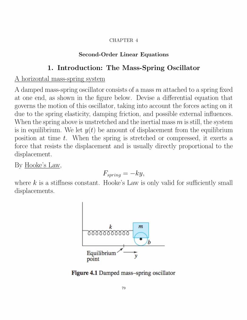
A damped mass-spring oscillator consists of a mass m attached to a spring fixedat one end, as shown in the figure below. Devise a di↵erential equation thatgoverns the motion of this oscillator, taking into account the forces acting on itdue to the spring elasticity, damping friction, and possible external influences.When the spring above is unstretched and the inertial mass m is still, the systemis in equilibrium. We let y(t) be amount of displacement from the equilibriumposition at time t. When the spring is stretched or compressed, it exerts aforce that resists the displacement and is usually directly proportional to thedisplacement.

By Hooke’s Law,Fspring = �ky,

where k is a sti↵ness constant. Hooke’s Law is only valid for su�ciently smalldisplacements.

79

80 4. SECOND-ORDER LINEAR EQUATIONS

Mechanical systems also experience friction and for vibrational motion is pro-portional to velocity:

Ffriction = �bdy

dt= �by0,

where b � 0 is the damping coe�cient. Any other forces on the oscillator areregarded as external to the system. We lump all such forces together into asingle, known fuction Fext(t). Then the DE for the mass-spring oscillator is

my00 = �ky � by0 + Fext

ormy00 + by0 + ky = Fext.

If b = Fext(t) = 0, this DE becomes the equation of simple harmonic motion

my00 + ky = 0,

or

y00 + �2y = 0, � =

rk

m,

which has a solution of the form

y(t) = cos �t.

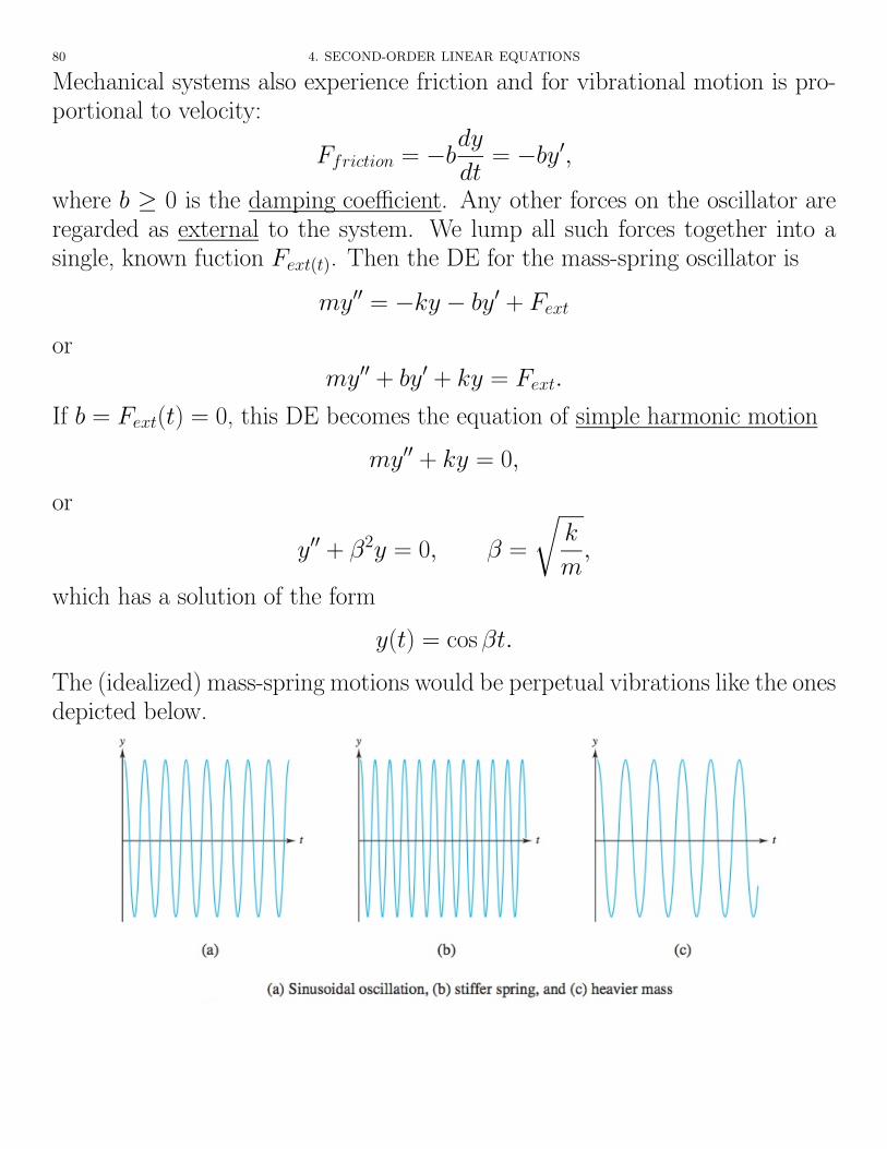
The (idealized) mass-spring motions would be perpetual vibrations like the onesdepicted below.

2. HOMOGENEOUS LINEAR EQUATIONS: THE GENERAL SOLUTION 81

These vibrations resemble sinusoidal functions, with their amplitude depend-ing on the initial displacement and velocity. The frequency of the oscillationsincreases for sti↵er springs but decreases for heavier masses.

Definition. Any DE of the form

a(t)y00 + b(t)y0 + c(t)y = g(t)

where a(t), b(t), c(t), and g(t) are continuous on some interval I , a(t) 6= 0 onI , is a second-order linear DE.

Any DE of the form(⇤) ay00 + by0 + cy = 0

where a, b, and c are constants, a 6= 0, is a second-order homogeneous linear

DE with constant coe�cients.

Goal: To solve (⇤) for all possible values of a, b, and c.

For understanding the math procedures and theory for solving (⇤), we willconsistently compare it with mass-spring paradigm:

[inertia]⇥ y00 + [damping]⇥ y0 + [sti↵ness]⇥ y = Fext.

2. Homogeneous Linear Equations: The General Solution

Example.

(1) y00 � y0 = 0.

Let x = y0. Then the DE becomes

x0 � x = 0,

a first-order linear DE with a specific, not general, solution

x = et.

Theny0 = et =)


y =

Zet dt = et

is a solution.

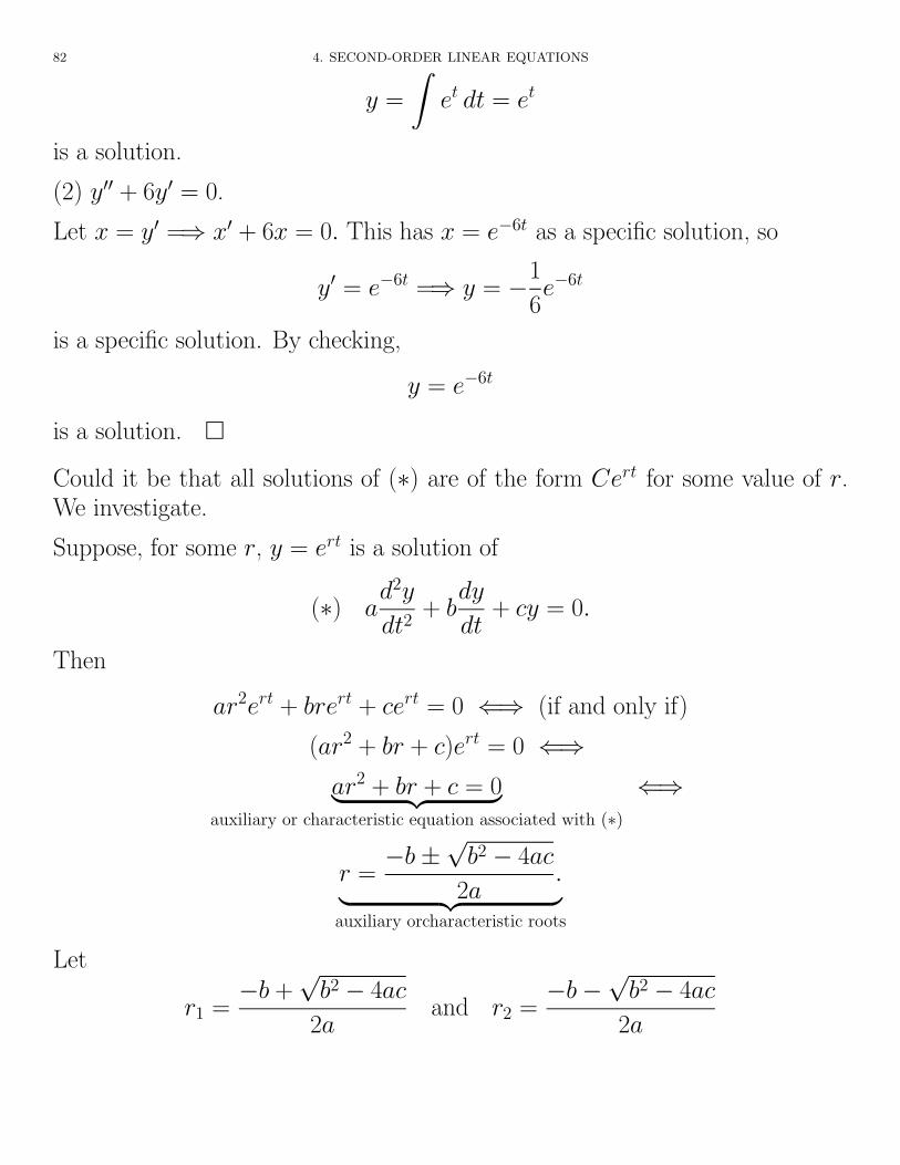
(2) y00 + 6y0 = 0.

Let x = y0 =) x0 + 6x = 0. This has x = e�6t as a specific solution, so

y0 = e�6t =) y = �1

6e�6t

is a specific solution. By checking,

y = e�6t

is a solution. ⇤

Could it be that all solutions of (⇤) are of the form Cert for some value of r.We investigate.

Suppose, for some r, y = ert is a solution of

(⇤) ad2y

dt2+ b

dy

dt+ cy = 0.

Then

ar2ert + brert + cert = 0 () (if and only if)

(ar2 + br + c)ert = 0 ()ar2 + br + c = 0| {z }

auxiliary or characteristic equation associated with (⇤)

()

r =�b ±

pb2 � 4ac

2a.

| {z }auxiliary orcharacteristic roots

Let

r1 =�b +

pb2 � 4ac

2aand r2 =

�b�p

b2 � 4ac

2a


Note, if the discriminant � = b2 � 4ac = 0, then r1 = r2 = � b

2a, giving the

characteristic equation a double or repeated root of multiplicity 2.

We have:

Lemma. ert is a solution of (⇤) () r is a root of ar2 + br + c = 0.

Note. The same is true for Cert.

But are there still other solutions?

Note that

r1 + r2 = �b

aand r1r2 =

c

a.

Then

ay00 + by0 + cy = 0 ()

y00 +b

ay0 +

c

ay = 0 ()

y00 � (r1 + r2)y0 + r1r2y = 0 ()

(y0 � r2xy)0 � r1(y0 � r2y) = 0.

Now let x = y0 � r2y. Then

x0 � r1x = 0,

which has the general solution x = k1er1t for k1 2 R. Substituting this solutioninto x = y0 � r2y,

y0 � r2y = k1er1t ()

e�r2ty0 � r2e�r2ty = k1e

r1te�r2t ()

(#)d

dt

he�r2ty

i= k1e

(r1�r2)t.

Suppose r1 6= r2. Then, integrating,

e�r2ty =

Zk1e

(r1�r2)t dt + k2 =k1

r1 � r2e(r1�r2)t + k2 ()


y(t) =k1

r1 � r2er1t + k2e

r2t,

with k1 and k2 arbitrary constants.

Letting c1 =k1

r1 � r2and c2 = k2,

y(t) = c1er1t + c2e

r2t

is a solution of (⇤) for all values of c1 and c2.

But what does this mean if r1 and/or r2 is complex? Also, what about the caseof r1 = r2?

Case 1 : r1 and r2 real, r1 6= r2.

For this case, we have established that all solutions of (⇤) are of the form

y(t) = c1er1t + c2e

r2t.

Also, any function written in the above form is a solution of

y00 � (r1 + r2)y0 + r1r2y = 0

since

(c1er1t + c2e

r2t)00 � (r1 + r2)(c1er1t + c2e

r2t)0 + r1r2(c1er1t + c2e

r2t) =

c1r21e

r1t + c2r22e

r2t � c1r21e

r1t � c2r1r2er2t � c1r1r2e

r1t

� c2r22e

r2t + c1r1r2er1t + c2r1r2e

r2t = 0.


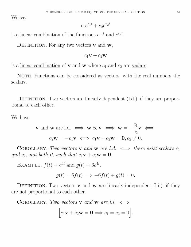
We say

c1er1t + c2e

r2t

is a linear combination of the functions er1t and er2t.

Definition. For any two vectors v and w,

c1v + c2w

is a linear combination of v and w where c1 and c2 are scalars.

Note. Functions can be considered as vectors, with the real numbers thescalars.

Definition. Two vectors are linearly dependent (l.d.) if they are propor-tional to each other.

We have

v and w are l.d. () w / v () w = �c1

c2v ()

c2w = �c1v () c1v + c2w = 0, c2 6= 0.

Corollary. Two vectors v and w are l.d. () there exist scalars c1

and c2, not both 0, such that c1v + c2w = 0.

Example. f(t) = e4t and g(t) = 6e4t.

g(t) = 6f(t) =) �6f(t) + g(t) = 0.

Definition. Two vectors v and w are linearly independent (l.i.) if theyare not proportional to each other.

Corollary. Two vectors v and w are l.i. ()hc1v + c2w = 0 =) c1 = c2 = 0

i.


Example. f(t) = et and g(t) = sin t.

These are clearly l.i., since if f(t) = kg(t),ht = 1 =) e = k sin 1 =) k ⇡ 3.23

iand

ht = 2 =) e2 = k sin 2 =) k ⇡ 8.126

i,

giving a contradiction.

Definition. For a second-order homogeneous linear DE, two l.i. solutionsare called a fundamental set of solutions.

Theorem (Distinct Real Characteristic Roots & General Solution). If thecharacteristic equation for

(⇤) ay00 + by0 + cy = 0

has the distinct real roots r1 and r2, then er1t and er2t are linearly indepen-dent solutions of (⇤) on the interval (�1,1). Furthermore,

y(t) = c1er1t + c2e

r2t,

where c1 and c2 are arbitrary constants, is a general solution on (�1,1).Example.

(1) Solve y00 = 5y0 + 24y. This is equivalent to

y00 � 5y0 � 24y = 0.

For the characteristic equation,

r2 � 5r � 24 = (r � 8)(r + 3) = 0 () r = 8 or r = �3.

Then the general solution is

y(t) = c1e8t + c2e

�3t.


(2) Solve y00 + 3y0 = 0.


r2 + 3r = r(r + 3) = 0 () r = �3 or r = 0.


y(t) = c1e�3t + c2e

0t = c1e�3t + c2.

Initial Value Problems

Suppose in (⇤), a = 1 and b = c = 0, yielding the DE y00 = 0. Then the graphof y(t) is simply a straight line and is uniquely determined by specifying a pointon the line,

y(t0) = Y0

and the slope of the line,y0(t0) = Y1.

The next theorem states that this idea transfers to the more general equation(⇤).

Theorem (1 — Existence and Uniqueness: Homogeneous Case). For anyreal numbers a(6= 0), b, c, t0, Y0, and Y1, there exists a unique solution tothe IVP

(⇤⇤) ay00 + by0 + cy = 0, y(t0) = Y0, y0(t0) = Y1.

The solution is valid for all t 2 (�1, +1).

But further,

Theorem (2 — Representation of Solutions to an IVP). If y1(t) and y2(t)are any two solutions of (⇤⇤) that are l.i. (i.e., a fundamental set ofsolutions) on (�1, +1), then unique constants c1 and c2 can always befound so that c1y1(t) + c2y2(t) satisfies the IVP (⇤⇤) on (�1, +1).

The proof of this theorem needs the following technical lemma.


Definition (Wronksian). The function

W (t) = W [y1, y2](t) =

��y1(t) y2(t)y01(t) y02(t)

�� = y1y02 � y01y2

where y1 and y2 are any di↵erentiable functions of t, is called the Wronksian ofy1 and y2.

Lemma (1— A condition for Linear Dependence of Solutions). For any realnumbers a(6= 0), b, and c, if y1(t) and y2(t) are any two solutions of (⇤) on(�1, +1) and if the equality

(#) W [y1, y2](⌧ ) = 0

holds at any point ⌧ , then y1 and y2 are l.d. on (�1, +1).Proof.

(1) If y1(⌧ ) 6= 0, let =y2(⌧ )

y1(⌧ )and consider the solution to (⇤) given by

y(t) = y1(t). For the IC of (⇤⇤), we have, with the second equality followingfrom (#),

y(⌧ ) =y2(⌧ )

y1(⌧ )y1(⌧ ) = y2(⌧ ), y0(⌧ ) =

y2(⌧ )

y1(⌧ )y01(⌧ ) = y02(⌧ ),

which are the same as those of y2, so by uniqueness y2(t) = y1(t).

(2) If y1(⌧ ) = 0 but y01(⌧ ) 6= 0, then (#) implies y2(⌧ ) = 0. Let =y02(⌧ )

y01(⌧ ).

Again, for y(t) = y1(t), for the IC of (⇤⇤), we have

y(⌧ ) =y02(⌧ )

y01(⌧ )y1(⌧ ) = 0 = y2(⌧ ), y0(⌧ ) =

y02(⌧ )

y01(⌧ )y01(⌧ ) = y02(⌧ ),

which are the same as those of y2, so by uniqueness y2(t) = y1(t).


(3) If y1(⌧ ) = y01(⌧ ) = 0, then y1(t) is a solution to (⇤) satisfying the ICy1(⌧ ) = y01(⌧ ) = 0. But y(t) ⌘ 0 is the unique solution to this IVP. Thusy1(t) ⌘ 0, and is then a constant multiple of y2(t). ⇤

We now prove Theorem 2:Proof.

We already know y(t) = c1y1(t) + c2y2(t) is a solution of (⇤).For (⇤⇤), we mustshow

y(t0) = c1y1(t0) + c2y2(t0) = Y0

andy0(t0) = c1y

01(t0) + c2y

02(t0) = Y1

But these are linear equations where the solutions are

c1 =Y0y02(t0)� Y1y2(t0)

y1(t0)y02(t0)� y01(t0)y2(t0)and c2 =

Y1y01t0)� Y0y01(t0)

y1(t0)y02(t0)� y01(t0)y2(t0),

provided the denominators are nonzero, which is the case here. ⇤

Example. Solve 2y00 + 7y0 + 5y = 0, y(0) = �2, y0(0) = 4.


2r2 + 7r + 5 = (2r + 5)(r + 1) = 0 () r = �5

2or r = �1.


y(t) = c1e�5

2t + c2e�t.

Then

y0(t) = �5

2c1e

�52t � c2e

�t.

From the initial conditions, we have

y(0) = c1 + c2 = �2

y0(0) = �5

2c1 � c2 = 4


Solving for c1 and c2 using elimination,

�3

2c1 = 2 =) c1 = �4

3=) c2 = �2

3.

This yields a particular solution of

y(t) = �4

3e�

52t � 2

3e�t.

Case 2 : r1 and r2 real, r1 = r2.

In solving

(⇤) ay00 + by0 + cy = 0,

we return to

(#)d

dt

he�r2ty

i= k1e

(r1�r2)t.

Since r1 = r2, this becomes, after renamimg k1 as c2,

d

dt

he�r2ty

i= c2.

Integrating, we have

e�r2ty = c2t + c1 =) y = (c1 + c2t)er2t =) (letting r = r2)

y(t) = c1ert + c2te

rt.

Theorem (Repeated Characteristic Roots & General Solution). If the char-acteristic equation for

(⇤) ay00 + by0 + cy = 0

has the real repeated root r, then ert and tert are linearly independentsolutions of (⇤) on the interval (�1,1). Furthermore,

y(t) = c1ert + c2te

rt,

where c1 and c2 are arbitrary constants, is a general solution on (�1,1).


Example.

(1) Solve 3y00 � 18y0 + 27y = 0.

This is equivalent toy00 � 6y0 + 9y = 0.


r2 � 6r + 9 = (r � 3)2 = 0 () r = 3, 3.


y(t) = c1e3t + c2te

3t.

(2) Solve y00 + 8y0 + 16y = 0, y(0) = 4, y0(0) = 0.


r2 + 8r + 16 = (r + 4)2 = 0 () r = �4,�4.


y(t) = c1e�4t + c2te

�4t.

Theny0(t) = �4c1e

�4t + c2e�4t � 4c2te

�4t.

From the initial conditions, we have

y(0) = c1 = 4

y0(0) = �4c1 + c2 = 0

Solving for c1 and c2 using substitution,

c2 = 4c1 = 16.

This yields a particular solution of

y(t) = 4e�4t + 16te�4t.


A Question:

For second-order homogeneous linear DE’s, do linear combinations of solutionsalways give another solution?

Suppose f 00 exists on an interval J = (↵,�). We say f is twice di↵erentiableon J . Further, suppose a(t), b(t), and c(t) are continuous on J . We define thedi↵erential operator L by

L[f ] = af 00 + bf 0 + cf.

This is a function whose domain is the set of twice di↵erentiable functions on

J . The range is a subset of the continuous functions on J .Letting D =d

dtand

D2 =d2

dt2, we have

L = aD2 + bD + c,

yielding

L[f ] = (aD2 + bD + c)f

= aD2f + bDf + cf

= af 00 + bf 0 + cf

With this notation and a, b, and c constants,

(⇤) becomes L[y] = 0.


L is a linear di↵erential operator in that, for f and g twice di↵erentiable and �and � continuous coe�cients,

L[�f ] = �L[f ] and

L[f + g] = L[f ] + L[g], or equivalently,

L[�f + �g] = �L[f ] + �L[g].

Proof.

L[�f + �g] = a(�f + �g)00 + b(�f + �g)0 + c(�f + �g)

= a�f 00 + a�g00 + b�f 0 + b�g0 + c�f + c�g

=⇥�(af 00 + bf 0 + cf)

⇤+

⇥�(ag00 + bg0 + cg)

⇤

= �L[f ] + �L[g].

⇤Note.

(1) Integration is also a linear operator.

(2) sin, cos, tan, exp, and ln are not linear operators, e.g.,

sin(a + b) 6= sin a + sin b.

Theorem (3 — Superposition Principal). If y1(t) and y2(t) are solutionsof

(⇤) ay00 + by0 + cy = 0

on (�1,1), then so is the linear combination

c1y1(t) + c2y2(t),

regardless of the values of the constants c1 and c2.

Proof. Let y1(t) and y2(t) be solutions of L[y] = 0 on (�1,1) whereL = aD2 + bD + c. Then L[y1(t)] = 0 and L[y2(t)] = 0 for all �1 < t < 1.Thus for all constants c1 and c2,

L[c1y1(t) + c2y2(t)] = c1L[y1(t)] + c2L[y2(t)] = c1 · 0 + c2 · 0 = 0,

so c1y1(t) + c2y2(t) is also a solution. ⇤


Problem (Page 166 # 40).

Solve y000 � 7y00 + 7y0 + 15y = 0.

Solution. We informally expand on our method. The associated charac-teristic equation is

r3 � 7r2 + 7r + 15 = 0.

We use synthetic division (Horner’s method) to find the roots.

�1 1 �7 7 15�1 8 �15

1 �8 15 |0Thus we have r = �1 as a root with the remaining roots being roots of

r2 � 8r + 15 = (r � 5)(r � 3) = 0,

namely r = 5 and r = 3. Thus e�t, e5t, and e3t are linearly independentsolutions yielding a general solution of

y(t) = c1e�t + c2e

5t + c3e3t.

⇤

3. Auxiliary Equations with Complex Roots

Case 3 : r1 and r2 are conjugate complex roots.

The solution to the characteristic equation is

r =�b ±

pb2 � 4ac

2awith b2 � 4ac < 0.

Then

r =�b ±

p�1p

4ac� b2

2a= � b

2a± i

p4ac� b2

2awith 4ac� b2 > 0.

Let

↵ = � b

2aand � =

p4ac� b2

2a.

3. AUXILIARY EQUATIONS WITH COMPLEX ROOTS 95

Then, renaming r1 and r2, the two conjugate complex roots of the characteristicequation are

r = ↵ + i� and r = ↵� i�.

Also,↵ = <r = <r, � = =r, and � � = =r.

We first consider the simple harmonic oscillator we began with:

(⇤⇤) y00 + �2y = 0, y(t0) = 0, y0(t0) = 0, � 6= 0.

It is clear that y(t) ⌘ 0 is a solution of (⇤⇤). But are there others?

Suppose u(t) is any solution of (⇤⇤). Then

u00(t) + �2u(t) = 0, u(t0) = 0, u0(t0) = 0.

So

2u0(t)⇥u00(t) + �2u(t)

⇤= 0 =)

Z t

t0

2u0(s)⇥u00(s) + �2u(s)

⇤ds =

Z t

t0

0 ds =)n

[u0(s)]2 + �2[u(s)]2o��

t

t0= 0 =)

[u0(t)]2 + �2[u(t)]2 � [u0(t0)]2 � �2[u(t0)]

2 = 0 =)(from IC) [u0(t)]2 + �2[u(t)]2 = 0 =)

u(t) = 0.

Thus we have

Lemma (1). Let t0, � be real numbers, where � 6= 0. Then the IVP

(⇤⇤) y00 + �2y = 0, y(t0) = 0, y0(t0) = 0

has the unique solution y(t) ⌘ 0 on (�1,1).


Now consider

(⇤ ⇤ ⇤) y00 + �2y = 0, y(t0) = y0, y0(t0) = y1, � 6= 0.

Suppose y(t) and ey(t) are two solutions of (⇤ ⇤ ⇤). Consider

u(t) = y(t)� ey(t).

By Superposition, u(t) is a solution of

y00 + �2y = 0.

Also,u(t0) = y(t0)� ey(t0) = y0 � y0 = 0

andu0(t0) = y0(t0)� ey 0(t0) = y1 � y1 = 0 =)

u(t) is a solution of (⇤⇤), so u(t) ⌘ 0. Then y(t) = ey(t). We have proven

Lemma (2). Let t0, y0, y1, and � be real numbers, where � 6= 0. If theIVP

(⇤ ⇤ ⇤) y00 + �2y = 0, x(t0) = y0, y0(t0) = y1

has a solution on (�1,1), then it is unique.

Question: Does (⇤ ⇤ ⇤) always have a solution?

For � 6= 0, we have an undamped mass-spring system which suggests repetitiousbehavior.

Suppose y(t) = cos �t. Then

y00 + �2y =d2

dt2cos �t + �2 cos �t = ��2 cos �t + �2 cos �t = 0,

so y(t) = cos �t is a solution of y00 + �2y = 0.

Similarly, y(t) = sin �t is also a solution.


Then, by superposition, anything of the form

(##) y(t) = c1 cos �t + c2 sin �t

is also a solution of y00 + �2y = 0.

But do these solutions satisfy the IC of (⇤ ⇤ ⇤)?For (##) to be a solution of (⇤ ⇤ ⇤), we need, noting

y0(t) = �c1� sin �t + c2� cos �t,

y(t0) = c1 cos �t0 + c2 sin �t0 = y0 and

y0(t0) = �c1� sin �t0 + c2� cos �t0 = y1

would have to have a solution for c1 and c2. In fact,

c1 = y0 cos �t0 �y1

�sin �t0 and

c2 = y0 sin �t0 +y1

�cos �t0.

Thusy(t) = c1 cos �t + c2 sin �t

with c1 and c2 as above is a solution of (⇤ ⇤ ⇤). By Lemma 2, it is the onlysolution. We have proven

Theorem (Simple Harmonic Oscillator and Solutions).

For any real numbers y1, y2, �, where � 6= 0, there exists a unique solutionof

(⇤ ⇤ ⇤) y00 + �2y = 0, y(t0) = y0, y0(t0) = y1.

This solution can be expressed in the form

y(t) = c1 cos �t + c2 sin �t,

where the constants c1 and c2 are uniquely determined by y0 and y1.


We return to(⇤) ay00 + by0 + cy = 0,

which we rewrite as

y00 +b

ay0 +

c

ay = 0.

Since we are assuming (⇤) has characteristic roots

r = ↵ + i� and r = ↵� i�,

we haveb

a= �(r + r) = �2↵

and c

a= r · r = (↵ + i�) · (↵� i�) = ↵2 + �2.

Then(⇤0) y00 � 2↵y0 + (↵2 + �2)y = 0

has the same solutions as (⇤).If � = 0, we have repeated roots, and from the previous theorem,

y(t) = c1e↵t + c2te

↵t

is a general solution =) e↵t is a solution.

Although e↵t is not a solution of (⇤0) since � 6= 0, every solution y(t) for (⇤0)can be written as

y(t) = e↵tx(t)

where

x(t) =y(t)

e↵t.


Substituting y(t) = e↵tx(t) into (⇤0),y00 � 2↵y0 + (↵2 + �2)y =

d2

dt2(e↵tx)� 2↵

d

dt(e↵tx) + (↵2 + �2)(e↵tx) =

d

dt[e↵tx0 + ↵e↵tx]� 2↵(e↵tx0 + ↵e↵tx) + ↵2e↵tx + �2e↵tx =

e↵tx00 + ↵e↵tx0 + ↵e↵tx0 + ↵2e↵tx� 2↵e↵tx0 + ↵2e↵tx� 2↵2e↵tx + �2e↵tx =

e↵tx00 + �2e↵tx =

e↵t(x00 + �2x) = 0 ()x00 + �2x = 0.

Thus, every solution of (⇤0) can be expressed as y(t) = e↵tx(t) where x(t) is asolution of x00 + �2x = 0.

Theorem (Complex Conjugate Roots and General Solution).

If the characteristic equation for

(⇤) ay00 + by0 + cy = 0

has the complex roots ↵ ± i� (� 6= 0), then e↵t cos �t and e↵t sin �t are l.i.solutions of (⇤) on (�1,1). A general solution on (�1,1) is

y(t) = c1e↵t cos �t + c2e

↵t sin �t,

where c1 and c2 are arbitrary constants.


Example.

(1) Solvey00 + 2y0 + 5y = 0, y(0) = 1, y0(0) = 1.

The associated characteristic equation

r2 + 2r + 5 = 0

has roots

r =�2 ±

p4� 20

2=�2 ± 4i

2= �1 ± 2i.

Let ↵ = �1, � = 2. Then

y(t) = c1e�t cos 2t + c2e

�t sin 2t

is the general solution and

y0(t) = �2c1e�t sin 2t� c1e

�t cos 2t + 2c2e�t cos 2t� c2e

�t sin 2t.

Theny(0) = c1 = 1 and

y0(0) = �c1 + 2c2 = �1 + 2c2 = 1 =) c2 = 1.

Thus the solution to the IVP is

y(t) = e�t cos 2t + e�t sin 2t.

Referring back to the unforced mass-spring oscillator

[inertia]⇥ y00 + [damping]⇥ y0 + [sti↵ness]⇥ y = 0

ormy00(t) + by0(t) + ky(t) = 0,

the exponential decay rate is ↵ = � b

2mand the angular frequency is � =

p4mk � b2

2m. Since b = 2 <

p4mk =

p20, this is an example of an under-

damped oscillator.


(2) Solvey00 + 2y0 + 10x = 0, y(0) = 1, y0(0) = 0.


r2 + 2r + 10 = 0

has roots

r =�2 ±

p4� 40

2=�2 ± 6i

2= �1 ± 3i.

Let ↵ = �1, � = 3. Then

y(t) = c1e�t cos 3t + c2e

�t sin 3t

is the general solution and

y0(t) = �3c1e�t sin 3t� c1e

�t cos 3t + 3c2e�t cos 3t� c2e

�t sin 3t.


y0(0) = �c1 + 3c2 = �1 + 3c2 = 0 =) c2 =1

3.


y(t) = e�t cos 3t +1

3e�t sin 3t.

Maple. See oscillate.mw or oscillate.pdf.


4. Nonhomogeneous Equations: The Method of UndeterminedCoe�cients

A second-order nonhomogeneous linear DE with constant coe�cients is an equa-tion of the form ay00+ by0+ cy = f(t) where a 6= 0 and f is any function otherthan the zero function.

Example. y00 � y = t.

By inspection, y = �t is a solution, called a particular solution.

Theorem (Solutions of Second-Order Nonhomogeneous Equations). A gen-eral solution of

(⇤) ay00 + by0 + cy = f(t)

on an interval J isy(t) = yh(t) + yp(t),

where yh(t) is a general solution of

ay00 + by0 + cy = 0

and yp(t) is any particular solution of (⇤) on J .

Proof. We rewrite (⇤) as L[y] = f(t), and let yp(t) be any particularsolution of (⇤) on J (i,e., for each t 2 J).

Suppose y(t) is some other solution of (⇤) on J =) L[y] = f(t). Then

L[y(t)� yp(t)] = L[y(t)]� L[yp(t)] = f(t)� f(t) = 0,

so y(t)� yp(t) is a solution of the associated homogeneous equation L[y] = 0.

Let yh(t) = y(t)� yp(t) (h for homogeneous)=)y(t) = yh(t) + yp(t).

Thus any solution of (⇤) can be written in this form.

On the other hand,

L[yh(t) + yp(t)] = L[yh(t)] + L[yp(t)] = f(t) + 0,

so anything of the form yh(t) + yp(t) is a solution of (⇤). ⇤

4. NONHOMOGENEOUS EQUATIONS: THE METHOD OF UNDETERMINED COEFFICIENTS 103

Finding Particular Solutions – Method of Undetermined Coe�cients

This method is used when f(t) is an l.c. of

(1) exponentials (ert)

(2) polynomials

(3) sin or cos

(4) products of the above

Example.

(1) Solve y00 � y = 3e�2t.

r2 � 1 = (r + 1)(r � 1) = 0 =) r = ±1.

yh(t) = c1et + c2e

�t.

For the particular solution:L[y] = 3e�2t.

We guess

L[Ae�2t] = 3e�2t =)4Ae�2t �Ae�2t = 3e�2t =)3Ae�2t = 3e�2t =) A = 1

Thenyp(t) = e�2t =)

y(t) = c1et + c2e

�t + e�2t.


(2) Solve y00 + 3y0 + 2y = 2t2 + 3t + 1.

r2 + 3r + 2 = (r + 1)(r + 2) = 0 =) r = �1,�2.

yh(t) = c1e�t + c2e

�2t.

For the particular solution:

L[y] = 2t2 + 3t + 1.

We guess

L[At2 + Bt + C] = 2t2 + 3t + 1 =)

2A + 3(2At + B) + 2(At2 + Bt + C) =

2At2 + (6A + 2B)t + (2A + 3B + 2C) = 2t2 + 3t + 1 =)2A = 2 =) A = 1

6A + 2B = 3 =) 2B = �3 =) B = �3

2

2A + 3B + 2C = 1 =) 2C =7

2=) C =

7

4Then

yp(t) = t2 � 3

2t +

7

4=)

y(t) = c1e�t + c2e

�2t + t2 � 3

2t +

7

4.


(3) Solve y00 � y0 � y = sin t.

r2 � r � 1 = 0 =) r =1 ±

p1 + 4

2=

1 ±p

5

2.

yh(t) = c1e1+p

52 t + c2e

1�p

52 t.

For the particular solution:L[y] = sin t.

We guess

L[A sin t] = sin t =)

�A sin t�A cos t�A sin t = �A(2 sin t + cos t) = sin t =)� 2A = 1 and �A = 0.

But this is impossible. A better guess is

L[A sin t + B cos t] = sin t =)

(�A sin t�B cos t)� (A cos t�B sin t)� (A sin t + B cos t) =

(�2A + B) sin t + (�A� 2B) cos t = sin t =)�2A + B = 1 and �A� 2B = 0 =)

A = �2B =) 4B + B = 1 =) 5B = 1 =)B =

1

5=) A = �2

5.

Then

yp(t) = �2

5sin t +

1

5cos t =)

y(t) = c1e1+p

52 t + c2e

1�p

52 t � 2

5sin t +

1

5cos t.


Method of Undetermined Coe�cients – Advanced

Example. Solve y00 � y = 2e�t.

From Example 1,yh(t) = c1e

t + c2e�t.

For the particular solution to

L[y] = 2e�t,

we guessy(t) = Ae�t =)

y0(t) = �Ae�t =)y00(t) = Ae�t =)

L[y] = Ae�t �Ae�t = 0 6= 2e�t.

We are left without an equation to solve for A. The problem is that a termof the trial solution is similar to a solution of the homogeneous equation. Theremedy is to multiply the trial solution by the smallest power of t so that is nolonger the case. We guess

y(t) = Ate�t =)y0(t) = Ae�t �Ate�t =)

y00(t) = �Ae�t �Ae�t + Ate�t =)L[y] = �2Ae�t + Ate�t �Ate�t = �2Ae�t = 2e�t =)

A = �1.

Thenyp(t) = �te�t

and the final solution is

y(t) = c1et + c2e

�t � te�t.


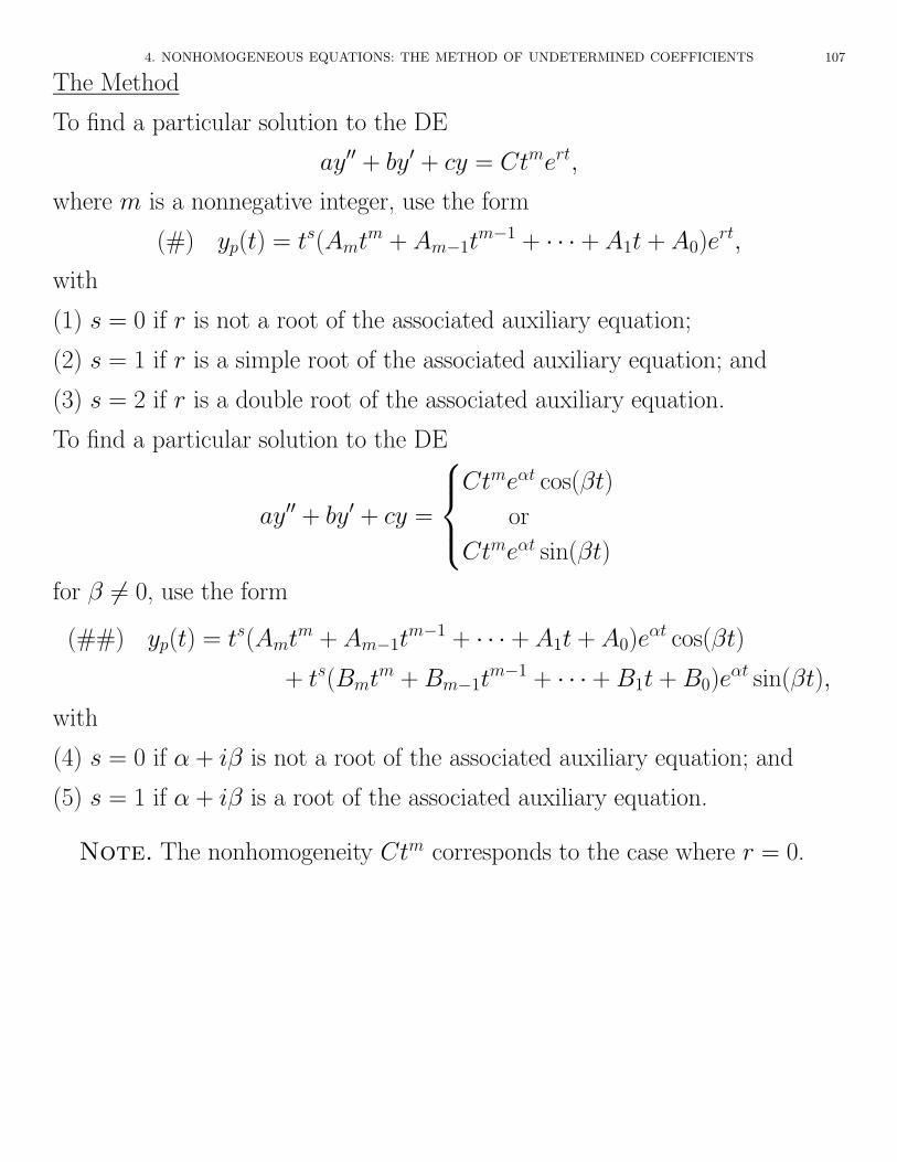
The Method

To find a particular solution to the DE

ay00 + by0 + cy = Ctmert,

where m is a nonnegative integer, use the form

(#) yp(t) = ts(Amtm + Am�1tm�1 + · · · + A1t + A0)e

rt,

with

(1) s = 0 if r is not a root of the associated auxiliary equation;

(2) s = 1 if r is a simple root of the associated auxiliary equation; and

(3) s = 2 if r is a double root of the associated auxiliary equation.


ay00 + by0 + cy =

8><

>:

Ctme↵t cos(�t)

or

Ctme↵t sin(�t)

for � 6= 0, use the form

(##) yp(t) = ts(Amtm + Am�1tm�1 + · · · + A1t + A0)e

↵t cos(�t)

+ ts(Bmtm + Bm�1tm�1 + · · · + B1t + B0)e

↵t sin(�t),

with

(4) s = 0 if ↵ + i� is not a root of the associated auxiliary equation; and

(5) s = 1 if ↵ + i� is a root of the associated auxiliary equation.

Note. The nonhomogeneity Ctm corresponds to the case where r = 0.


Problem (Page 182 # 26). Solve y00 + 2y0 + 2y = 4te�t cos t.

Solution. The auxiliary equation is r2 + 2r + 2 =)

r =�2 ±

p4� 8

2=�2 ± 2i

2= �1 ± i =)

yh(t) = c1e�t cos t + c2e

�t sin t.

For the nonhomogeneous part, we need to use (##). With ↵ = �1 and � = 1,↵ + i� is a solution to the auxiliary equation, so from (5), s = 1 and

yp(t) = t⇥(A1t + A0) cos t + (B1t + B0) sin t

⇤e�t =

⇥(A1t

2 + A0t) cos t + (B1t2 + B0t) sin t

⇤e�t,

y0p(t) = �h�

(A1 �B1)t2 + (A0 �B0 � 2A1)t�A0

�cos t

+�(A1 + B1)t

2 + (A0 + B0 � 2B1)t�B0

�sin t

ie�t,

y00p(t) = 2h��B1t

2 + (�B0 � 2A1 + 2B1)t�A0 + B0 + A1

�cos t

+�A1t

2 + (A0 � 2A1 � 2B1)t�A0 �B0 + B1

�ie�t.

Then

(4B1t + 2B0 + 2A1)e�t cos t + (�4A1t� 2A0 + 2B1)e

�t sin t = 4te�t cos t,

so4B1 = 4 =) B1 = 1, B0 + A1 = 0, A1 = 0 =) B0 = 0,

�A0 + B1 = 0 =) A0 = 1.

Thusyp(t) = (t cos t + t2 sin t)e�t =)

y(t) = yh(t) + yp(t) = c1e�t cos t + c2e

�t sin t + (t cos t + t2 sin t)e�t.

⇤


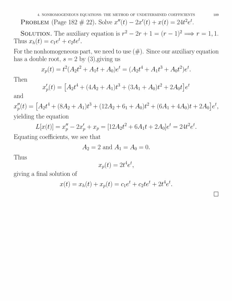
Problem (Page 182 # 22). Solve x00(t)� 2x0(t) + x(t) = 24t2et.

Solution. The auxiliary equation is r2 � 2r + 1 = (r � 1)2 =) r = 1, 1.Thus xh(t) = c1et + c2tet.

For the nonhomogeneous part, we need to use (#). Since our auxiliary equationhas a double root, s = 2 by (3),giving us

xp(t) = t2(A2t2 + A1t + A0)e

t = (A2t4 + A1t

3 + A0t2)et.

Thenx0p(t) =

⇥A2t

4 + (4A2 + A1)t3 + (3A1 + A0)t

2 + 2A0t⇤et

and

x00p(t) =⇥A2t

4 + (8A2 + A1)t3 + (12A2 + 61 + A0)t

2 + (6A1 + 4A0)t + 2A0

⇤et,

yielding the equation

L[x(t)] = x00p � 2x0p + xp = [12A2t2 + 6A1t + 2A0]e

t = 24t2et.

Equating coe�cients, we see that

A2 = 2 and A1 = A0 = 0.

Thusxp(t) = 2t4et,

giving a final solution of

x(t) = xh(t) + xp(t) = c1et + c2te

t + 2t4et.

⇤


Problem (Page 182 # 36). Find a particular solution to

y(4) � 3y00 � 8y = sin t.Solution.

We use the form (##) with ↵ = 0 and � = 1. We note that i is not a root ofthe auxiliary equation r4 � 3r2 � 8 = 0, so we choose s = 0. Then

yp(t) = A0 cos t + B0 sin t =)y0p(t) = �A0 sin t + B0 cos t =)y00p(t) = �A0 cos t�B0 sin t =)y000p (t) = A0 sin t�B0 cos t =)y(4)

p (t) = A0 cos t + B0 sin t.

Theny(4)

p � 3y00p � 8yp = �4A0 cos t� 4B0 sin t = sin t =)

A0 = 0 and B0 = �1

4=)

yp(t) = �sin t

4.

⇤

5. THE SUPERPOSITION PRINCIPLE AND UNDETERMINED COEFFICIENTS REVISITED 111

5. The Superposition Principle and Undetermined Coe�cientsRevisited

Theorem (3 — Superposition Principal). Let y1(t) be a solution to

ay00 + by0 + cy = f1(t)

and y2(t) be a solution to

ay00 + by0 + cy = f2(t).

Then the linear combination

k1y1(t) + k2y2(t),

is a solution ofay00 + by0 + cy = k1f1(t) + k2f2(t)

regardless of the values of the constants k1 and k2.

Proof. Let y1(t) be a solution to ay00 + by0 + cy = f1(t) and y2(t) be asolution to ay00+by0+cy = f2(t) where L = aD2 +bD+c. Then L[y1(t)] = f1

and L[y2(t)] = f2. Thus for all constants k1 and k2,

L[k1y1(t) + k2y2(t)] = k1L[y1(t)] + k2L[y2(t)] = k1f1(t) + k2f2(t),

so k1y1(t) + k2y2(t) is a solution to

ay00 + by0 + cy = k1f1(t) + k2f2(t).

⇤


Example. Solve y00 � y = 2e�t � 4te�t + 10 cos 2t.

From a previous Example (1),

yh(t) = c1et + c2e

�t.

For the particular solution, we will use superposition. For

L[y] = (2� 4t)e�t,

we use (#) with s = 1 since �1 is a simple root of r2� 1 = 0. We thus choose

yp(t) = t(A + Bt)e�t = (At + Bt2)e�t =)y0p(t) = [A + (2B �A)t�Bt2]e�t =)

y00p(t) = [(2B � 2A) + (A� 4B)t + Bt2]e�t =)L[yp] = (2B � 2A)(e�t)� 4Bte�t = 2e�t � 4te�t =)

2B � 2A = 2 and � 4B = �4 =)B = 1 =) A = 0.

Thenyp(t) = t2e�t.

ForL[y] = 10 cos 2t,

we use (##) with m = 1, ↵ = 0, � = 2, and s = 0 since i is not a root ofr2 � 1 = 0, i.e,

yq(t) = A cos 2t + B sin 2t =)y00q = �4A cos 2t� 4B sin 2t =)

L[yq] = (�4A cos 2t� 4B sin 2A)� (A cos 2t + B sin 2t) =

� 5A cos 2t� 5B sin 2t = 10 cos 2t =)A = �2 and B = 0.

Thenyq(t) = �2 cos 2t =)

y(t) = yh(t) + yp(t) + yq(t) = c1et + c2e

�t + t2e�t � 2 cos 2t.


The next theorem addresses IVP’s:

Theorem (4 — Existence and Uniqueness: Nonhomogeneous Case). Forany ral numbers a(6= 0), b, c, t0,Y0, and Y1, suppose yp(t) is a particularsolution to

(⇤) ay00 + by0 + cy = f(t)

in an interval I containing t0 and that y1(t) and y2(t) are l.i. solutionsto the associated homogeneous equation in I. Then there exists a uniquesolution in I to the IVP

ay00 + by0 + cy = f(t), y(t0) = Y0, y0(t0) = Y1,

and it is given by

Y (t) = c1y1(t) + c2y2(t) + yp(t)

for the appropriate choice of constants c1 and c2

Problem (Page 187 # 2c). Given that y1(t) = cos t is a solution to

y00 � y0 + y = sin t

and y2(t) =e2t

3is a solution to

y00 � y0 + y = e2t,

use the superposition principle to find a solution to

y00 � y0 + y = 4 sin t + 18e2t.

Solution. Let g1(t) = sin t and g2(t) = e2t. Since

4 sin t + 18e2t = 4g1(t) + 18g2(t),

the functiony(t) = 4y1(t) + 18y2(t) = 4 cos t + 6e2t

is a solution toy00 � y0 + y = 4 sin t + 18e2t.

⇤


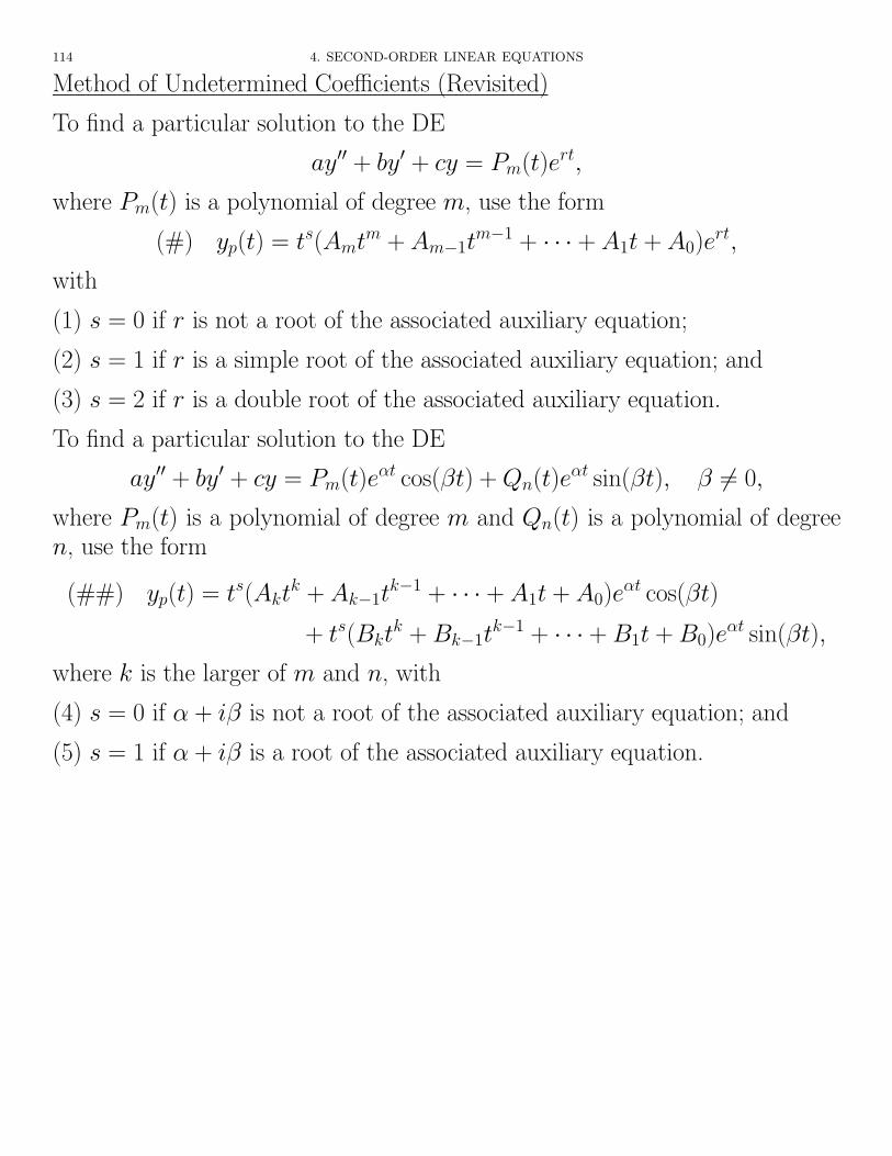
Method of Undetermined Coe�cients (Revisited)


ay00 + by0 + cy = Pm(t)ert,

where Pm(t) is a polynomial of degree m, use the form

(#) yp(t) = ts(Amtm + Am�1tm�1 + · · · + A1t + A0)e

rt,

with

(1) s = 0 if r is not a root of the associated auxiliary equation;

(2) s = 1 if r is a simple root of the associated auxiliary equation; and

(3) s = 2 if r is a double root of the associated auxiliary equation.


ay00 + by0 + cy = Pm(t)e↵t cos(�t) + Qn(t)e↵t sin(�t), � 6= 0,

where Pm(t) is a polynomial of degree m and Qn(t) is a polynomial of degreen, use the form

(##) yp(t) = ts(Aktk + Ak�1t

k�1 + · · · + A1t + A0)e↵t cos(�t)

+ ts(Bktk + Bk�1t

k�1 + · · · + B1t + B0)e↵t sin(�t),

where k is the larger of m and n, with

(4) s = 0 if ↵ + i� is not a root of the associated auxiliary equation; and

(5) s = 1 if ↵ + i� is a root of the associated auxiliary equation.


Problem (Page 188 # 22). Find a general solutiopn to

y00(x) + 6y0(x) + 10y(x) = 10x4 + 24x3 + 2x2 � 12x + 18.Solution.

The auxiliary equation r2 + 6r + 10 has roots

r =�6 ±

p36� 40

2=�6 ± 2i

2= �3 ± i.

Thusyh(x) = c1e

�3x cos x + c2e�3x sin x.

For a partcular solution, using (#) with r = s = 0, we choose

yp(x) = A4x4 + A3x

3 + A2x2 + A1x + A0 =)

y0p(x) = 4A4x3 + 3A3x

2 + 2A2x + A1 =)y00p(x) = 12A4x

2 + 6A3x + 2A2 =)

y00p + 6y0p + 10yp = 10A4x4 + (10A3 + 24A4)x

3 + (10A1 + 12A2 + 6A3)x2

+ (10A1 + 12A2 + 6A3)x + (10A0 + 6A1 + 2a2)

= 10x4 + 24x3 + 2x2 � 12x + 18 =)A4 = 1, A3 = 0, A2 = �1, A1 = 0, A0 = 2.

Thenyp(x) = x4 � x2 + 2,

so

y(x) = yh(x) + yp(x) = c1e�3x cos x + c2e

�3x sin x + x4 � x2 + 2.

⇤


Problem (Page 188 # 30). Solve the IVP

y00 + 2y0 + y = t2 + 1� et, y(0) = 0, y0(0) = 2.Solution.

The auxiliary equation r2 + 2r + 1 = 0 has r = 1 as a double root. Thus

yh(t) = c1e�t + c2te

�t.

From the superposition principle, we choose

yp(t) = A2t2 + A1t + A0 + B0e

t =)y0p(t) = 2A2t + A1 + B0e

t =)y00p(t) = 2a2 + B0e

t =)L[yp(t)] = A2t

2 + (A1 + 4A2)t + (A0 + 2A1 + 2A2) + 4B0et = t2 + 1� et =)

A2 = 1, A1 = �4A2 = �4, A0 = 1� aA1 � 2A2 = 7. B0 = �1

4.

Thus

yp(t) = t2 � 4t + 7� et

4=)

the general solution is

y(t) = yh(t) + yp(t) = c1e�t + c2te

�t + t2 � 4t + 7� et

4=)

y0(t) = �c1e�t + c2e

�t � c2te�t + 2t� 4� et

4.

For the initial conditions,

y(0) = c1 + 7� 1

4= 0 =) c1 = �27

4and

y0(0) = �c1 + c2 � 4� 1

4= 2 =) c2 = �1

2.


y(t) = yh(t) + yp(t) = �27

4e�t +�1

2te�t + t2 � 4t + 7� et

4.

⇤

6. VARIATION OF PARAMETERS 117

6. Variation of Parameters

This is a method for finding a particular solution for any second-order linearnonhomogeneous DE

(⇤) a(t)y00 + b(t)y0 + c(t)y = f(t)

where a, b, c, and f are continuous functions on an interval I , a(t) 6= 0 on I ,and where we are able to find a general solution to the associated homogeneousequation.

Example (First Order). Solve y0 + 4ty = 6e�2t2.

The associated homogeneous equation is

y0 + 4ty = 0.

µ = eR

4t dt = e2t2 =)

e2t2y0 + 4te2t2y = 0 =) d

dt

he2t2y

i= 0 =)

e2t2y = k =) yh(t) = ke�2t2

is a general solution to the homogeneous equation, with k as a parameter. Thuswe look for a particular solution of the form

yp(t) = v(t)e�2t2

by varying the parameter. Substituting into our DE,

y0p + 4typ = v0(t)e�2t2 + v(t)(�4te�2t2) + 4tv(t)e�2t2 = v0(t)e�2t2.

Then, by matching up with the original equation,

v0(t) = 6 =) v(t) = 6t.

Thenyp(t) = 6te�2t2 =)

y(t) = ke�2t2 + 6te�2t2 = (6t + k)e�2t2

is a general solution.


We now expand on this idea in finding particular solutions for second-orderequations. From Theorem 4 of the previous section, we know that what we arelooking for is out there.

Assume y1(t) and y2(t) are l.i. solutions of the homogeneous DE associatedwith (⇤). Then

yh(t) = c1y1(t) + c2y2(t)

is a general solution of the homogeneous DE. We need to find v1(t), v2(t) suchthat

yp(t) = v1(t)y1(t) + v2(t)y2(t)

is a solution of (⇤).y0p = (v1y

01 + v2y

02) + (v01y1 + v02y2),

y00p = (v1y001 + v2y

002) + (v01y

01 + v02y

02) +

d

dt(v01y1 + v02y2).

Supposev01y1 + v02y2 = 0.

Then the LHS (left-hand-side) of (⇤) is

ay00p = av1y001 + av2y002 + a(v01y01 + v02y

02)

+by0p = bv1y01 + bv2y02+cyp = cv1y1 + cv2y2

————————————————————

L[yp] = v1L[y1] + v2L[y2] + a(v01y01 + v02y

02)

Since y1 and y2 are solutions of the associated DE,

L[y1] = 0 and L[y2] = 0 =)L[yp] = a(v01y

01 + v02y

02).


Then yp will be a solution of (⇤) if also L[yp] = f , or altogether if the system

(⇤)

8<

:y1v01 + y2v02 = 0

y01v01 + y02v

02 =

f

ahas a solution for v01, v02.

To eliminate u02,

y1y02v01 + y2y02v

02 = 0

�y01y2v01 � y2y

02v02 = �fy2

a————————————

v01(y1y02 � y01y2) = �fy2

a.

Similarly, eliminating v01,

v02(y1y02 � y01y2) = �fy1

a.

Thus, the system has a solution if

W [y1, y2](t) = y1y02 � y01y2 6= 0.

But since y1(t) and y2(t) are l.i., Lemma 1 from Section 2 of this chapter saysthat this is always the case. Then the solutions of (⇤) are

v01(t) = �f(t)y2(t)

a(t)W (t)and v02(t) =

f(t)y1(t)

a(t)W (t)=)

v1(t) = �Z

f(t)y2(t)

a(t)W (t)dt and v2(t) =

Zf(t)y1(t)

a(t)W (t)dt =)

yp(t) = �y1(t)

Zf(t)y2(t)

a(t)W (t)dt + y2(t)

Zf(t)y1(t)

a(t)W (t)dt.


Method of Variation of Parameters

To find yp, a particular solution of

(⇤) a(t)y00 + b(t)y0 + c(t)y = f(t) :

(1) Findyh(t) = c1y1(t) + c2y2(t),

the solution of the homogeneous DE associated with (⇤).(2) Solve 8

<

:y1v01 + y2v02 = 0

y01v01 + y02v

02 =

f

afor v01(t) and v02(t).

(3) Find v1(t) and v2(t) by integration with 0 as the constants of integration.

(4) The particular solution is then

yp(t) = v1(t)y1(t) + v2(t)y2(t).

In solving the system of equations in (2), it is often useful to use

Theorem (Cramer’s Rule). If

��a bc d

�� = ad� bc 6= 0, the solution of

(ax + by = e

cx + dy = f

is

x =

��e bf d

��a bc d

��

and y =

��a ec f

��a bc d

��

.


Example.

(1) Solve y00 + y = tan t on⇣� ⇡

2,⇡

2

⌘.

r2 + 1 = 0 =) r2 = �1 =) r = ±i =) ↵ = 0 and � = 1 =)yh(t) = c1 cos t + c2 sin t =) y1(t) = cos t and y2(t) = sin t.

This yields the system of equations(

(cos t)v01 + (sin t)v02 = 0

�(sin t)v01 + (cos t)v02 = tan t

We use Cramer’s Rule to solve for v01 and v02.

v01 =

��0 sin t

tan t cos t

��

cos t sin t� sin t cos t

��

= � sin t tan t

v02 =

��cos t 0� sin t tan t

��

1= cos t tan t

v1(t) = �Z

sin t tan t dt = �Z

sin2 t

cos tdt = �

Z1� cos2 t

cos tdt =

Z(cos t� sec t) dt = sin t� ln(sec t + tan t)

v2(t) =

Zcos t tan t dt =

Zsin t dt = � cos t

Then

yp(t) = [sin t� ln(sec t + tan t)] cos t� cos t sin t = � cos t ln(sec t + tan t) =)y(t) = c1 cos t + c2 sin t� cos t ln(sec t + tan t)



(2) Solve y00 + 4y0 + 4y = te�2t.

r2 + 4r + 4 = (r + 2)2 = 0 =) r = �2,�2 =)yh(t) = c1e

�2t + c2te�2t =) y1(t) = e�2t and y2(t) = te�2t.

This yields the system of equations(

e�2tv01 + te�2tv02 = 0

�2e�2tv01 + (e�2t � 2te�2t)v02 = te�2t

We then divide each equation by e�2t to simplify.(

v01 + tv02 = 0

�2v01 + (1� 2t)v02 = t

We use Cramer’s Rule to solve for u01 and u02.

v01 =

��0 tt 1� 2t

��

1 t�2 1� 2t

��

=�t2

1= �t2

v02 =

��1 0�2 t

��

1= t

v1(t) = �Z

t2 dt = �t3

3and v2(t) =

Zt dt =

t2

2Then

yp(t) = �t3

3e�2t +

t2

2te�2t =

1

6t3e�2t =)

y(t) = c1e�2t + c2te

�2t +1

6t3e�2t


7. VARIABLE-COEFFICIENT EQUATIONS 123

7. Variable-Coe�cient Equations

We begin with an important theorem. In this theorem, we write the secondorder DE in what is called standard form.

Theorem (5 — Existence and Uniqueness of Solutions). Suppose p(t),q(t), and g(t) are continuous on an interval (a, b) that contains the pointt0. Then, for any choice of initial values Y0 and Y1, there exists a uniquesolution y(t) on the same interval (a, b) to the IVP

y00(t) + p(t)y0(t) + q(t)y(t) = g(t), y(t0) = Y0, y0(t0) = Y1.

Cauchy-Euler Equations

In general, a second-order linear homogeneous DE with non-constant coe�cients

a(t)y00 + b(t)y0 + c(t)y = 0

has solutions that cannot be expressed in terms of finitely many elementaryfunctions. Such equations often require power series solutions or numericaltechniques. An exception:

Definition (2 — Homogeneous Cauchy-euler Equations).

A second-order homogeneous Cauchy-Euler equation is an equation of the form

(⇤) at2y00 + bty0 + cx = 0

where a, b, c are constants.

We will use a technique di↵erent from that of the text here.


We first seek a solution on an interval where t > 0. We do a change of variable

t = eu (since t > 0).

Nowdt

du= eu = t,

so

(⇧) dy

du=

dy

dt· dt

du= t

dy

dt

and

d2y

du2=

d

du

⇣tdy

dt

⌘

= td

du

⇣dy

dt

⌘+

dy

dt· dt

du

= td2y

dt2· dt

du+

dt

du· dy

dt

= t2d2y

dt2+

dy

du=)

(⇧⇧) t2d2y

dt2=

d2y

du2� dy

du.

Then (⇤) becomes

a⇣d2y

du2� dy

du

⌘+ b

dy

du+ cy = 0

or

(#) ad2y

du2+ (b� a)

dy

du+ cy = 0.

The characteristic equation for (#) is then

ar2 + (b� a)r + c = 0,

called the Cauchy-Euler characteristic equation. Since (#) has constant coef-ficients, we use the 3 cases discussed above to find general solutions y(u). We


then find general solutions x(t) by using the reverse substitution

u = ln t.

We now seek a solution on an interval where t < 0. In this case, we use

�t = eu,

sody

du=

dy

dt· dt

du=

dy

dt(�eu) = t

dy

dt.

Thus (⇧) and (⇧⇧) remain the same as before, again yielding (#) as an equation.But now the reverse substitution is

u = ln(�t).

Putting the two solutions together, we have the

Method for Solving Homogeneous Cauchy-Euler Equations

To find a general solution of

(⇤) at2y00 + bty0 + cy = 0

on an interval that excludes t = 0, complete the following steps.

(1) Find a general solution of the associated equation

(#) ad2y

du2+ (b� a)

dy

du+ cy = 0.

(2) After completing Step 1, replace u with ln|t| and eu with |t|.


Example.

(1) Solve 3t2y00 + 11ty0 � 3y = 0, t 6= 0.


ar2 + (b� a)r + c = 3r2 + 8r � 3 = (3r � 1)(r + 3) = 0

has roots

r1 =1

3and r2 = �3.

Theny(u) = c1e

13u + c2e

�3u = c1(eu)

13 + c2(e

u)�3 =)y(t) = c1|t|

13 + c2|t|�3.

(2) Solve t2y00 + 3ty0 + 4y = 0, t > 0.


ar2 + (b� a)r + c = r2 + 2r + 4 = 0

has roots

r =�2 ±

p4� 16

2=�2 ± 2i

p3

2= �1 ±

p3i.

Let ↵ = �1 and � =p

3. Then

y(u) = c1e�u cos(

p3u) + c2e

�u sin(p

3u) =)y(t) = c1t

�1 cos(p

3 ln t) + c2t�1 sin(

p3 ln t).


(3) Solve 9t2y00 + 15ty0 + y = 0, t > 0, y(1) = 2, y0(1) =7

3.


ar2 + (b� a)r + c = 9r2 + 6r + 1 = (3r + 1)2 = 0

has roots

r1 = r2 = �1

3.

Theny(u) = c1e

�13u + c2ue�

13u =)

y(t) = c1t�1

3 + c2t�1

3 ln t =c1 + c2 ln t

t13

=)

y0(t) =t

13

⇣c2 · 1

t

⌘� (c1 + c2 ln t)1

3t�2

3

t23

=13t�2

3 [3c2 � c1 � c2 ln t]

t23

=

3c2 � c1 � c2 ln t

3t43


y0(1) =3c2 � c1

3=

3c2 � 2

3=

7

3=) 3c2 � 2 = 7 =) c2 = 3.


y(t) =2 + 3 ln t

t13

.

Documents

Second-Order Linear Equationsfacstaff.cbu.edu/wschrein/media/M231 Notes/M231C4.pdfSecond-Order Linear Equations 1. Introduction: The Mass-Spring Oscillator A horizontal mass-spring