Embed Size (px)
Citation preview

WWW.JAMK.FI
Design of a Solar ThermalPowered Cooling System
Olli Hurri
Bachelor’s Thesis
May 2011
Wellness Technology
Technology, Communication and Transport

DESCRIPTION
Author(s) Type of publication DateHURRI, Olli Bachelor’s Thesis 11.05.2011
Pages Language95 English
Confidential Permission for webpublication
() Until (x)TitleDESIGN OF A SOLAR THERMAL POWERED COOLING SYSTEM
Degree ProgrammeDegree Programme in Wellness Technology
Tutors(s)MATILAINEN, Jorma
Assigned byRobert Bosch GmbHDANNE, ThomasAbstract
The main objective of the thesis was to design a mechanical structure for a desiccantevaporative cooling, to apply solar thermal powered air conditioning systems in detachedhouses. The work was based on a process which was already proven thermally efficient byexperimental tests of a prototype. The thesis was carried out in the group “Solar Systems”which belongs to the “Corporate Research” unit of the company Robert Bosch GmbH.
In southern Europe, to maintain comfortable inside air conditions, inefficient electronicallydriven cooling methods are used in a large scale during the relatively hot summers.Simultaneously with high cooling demands, usually intensive solar radiation is present. Thedesiccant evaporative cooling is a sensible way to utilize the available solar thermal energyin the air conditioning systems, when an electrical cooling coefficient of performance of over20 can be reached.
The most critical factors of the design were pressure loss and size which are related to eachother. In general, the desiccant evaporative cooling systems were already in industrial use,but downscaling of the system led to several problems such as unacceptably high internalleakage and pressure drop. Thus, new solutions were needed for the small applications.
As an introduction, was an orientation to the thermal process behind the desiccantevaporative cooling. Then, the mechanical design was started with several estimations.During the design process, new construction concepts and mechanical solutions wereinvented. At the same time, besides the pressure loss, components such as heat exchangers,valves, fans, filters and water spray nozzles were optimized. During the optimization,various engineering tools were used and with each step the estimations of the variablesbecame more precise.
The design outcome is a conceptual 3D model of a construction that contains the optimizedcomponents of the desiccant evaporative cooling process in the required size. The pressureloss in the construction is calculated comprehensively. Due to that, the most mentionabledesign result is the proven competitiveness of the desiccant evaporative cooling system fordetached house use. Additionally, a noteworthy invention is a simple and effective valvemechanism to control the adsorption and desorption phases, which can be used in nearlyevery open cycle desiccant evaporative cooling system.
Keywordssolar energy, desiccant evaporative cooling, air ventilation
Miscellaneous

OPINNÄYTETYÖNKUVAILULEHTI
Tekijä(t) Julkaisun laji PäiväysHURRI, Olli Opinnäytetyö 11.05.2011
Sivumäärä Julkaisun kieli95 englanti
Luottamuksellisuus Verkkojulkaisulupamyönnetty
() saakka (x)Työn nimiAURINKOJÄÄHDYTYSJÄRJESTELMÄN OMAKOTITALOSOVELLUKSEN SUUNNITTELU
KoulutusohjelmaHyvinvointiteknologian koulutusohjelma
Työn ohjaajaMATILAINEN, Jorma
ToimeksiantajaRobert Bosch GmbHDANNE, ThomasTiivistelmä
Kuudessa tunnissa aurinko säteilee maailman aavikoille enemmän energiaa kuin kokoihmiskunta kuluttaa vuodessa. Kesäisin samainen energialähde aiheuttaa epämiellyttävänkuumuuden asuintiloihin esimerkiksi Etelä-Euroopassa. Huolimatta epämiellyttävänkuumuuden ja käytettävissä olevan aurinkoenergian samanaikaisuudesta, asuintilojajäähdytetään pääasiassa matalahyötysuhteisilla sähköteknologioilla. Globaalienympäristöongelmien, kuten ilmastonmuutoksen torjunnassa sähkönkulutuksenpienentäminen on avainasemassa. Ilmastoinnin osalta mahdollinen tulevaisuuden ratkaisukesäisen sähkökuorman alentamiseen on aurinkojäähdytys.
Saksassa Robert Bosch GmbH:n tutkimusyksikössä tehdyn opinnäytetyön aiheena oliaurinkoenergiaa hyödyntävän ilmastointikoneen omakotitalosovelluksen suunnittelu.Aurinkojäähdytys perustuu kuivaushaihdutusjäähdytykseen (DEC), joka käyttää auringonlämpöenergiaa kuivausaineen regenerointiin. Aurinkoenergian suoman hyödyn ansiostatehokas ilmastointi on mahdollista toteuttaa minimaalisella sähkönkulutuksella.
Opinnäytetyön suurin haaste oli DEC-prosessia kunnioittavan ja kooltaan omakotitaloonsopivan ilmastointikoneen suunnittelu. Keskeinen ongelma oli vaatimusten mukainentoisistaan riippuvien rakenteen ja painehäviön optimointi. Itse optimointi perustuijäähdytysprosessin ja ilmastointikoneen komponenttien teorian ohella fyysisen rakenteenideointiin, sekä toiminnallisten komponenttien suunnitteluun koneenrakennuksen javirtausdynamiikan keinoin.
Suunnittelutyön tuloksia ovat ensisijaiset vaatimukset täyttävät 3D-mallitomakotitalosovelluksesta, sekä järjestelmän optimoidut toiminnalliset komponentit.Suunnitellun järjestelmän painehäviö on määritetty kattavasti, jonka perusteellaaurinkojäähdytyksellä voidaan saavuttaa sähköinen hyötysuhde noin 29. Lisäksi tuloksenatäytyy mainita keksintö venttiilimekanismista, joka mahdollistaa matalahäviöisenilmavirtojen kontrolloinnin jokaisessa avoimessa DEC-sovelluksessa. Opinnäytetyön tulostennojalla voidaan aurinkojäähdytys omakotitalosovelluksissa todeta järkeväksi. Lisäksijärjestelmän yksinkertaista rakennetta ja työssä käytettyjä suunnittelulinjoja voidaankäyttää tukevana pohjana varsinaiselle tuotekehitykselle kohti energiatehokastailmastointia.
Avainsanat (asiasanat)aurinkojäähdytys, kuivaushaihdutusjäähdytys, ilmastointi
Muut tiedot

1
CONTENTS
1 INTRODUCTION . . . . . . . . . . . . . . . . . . . . . . . . . . . 5
1.1 Solar energy and cooling . . . . . . . . . . . . . . . . . . . . . . . . 5
1.2 Robert Bosch GmbH and CR/AEB2 . . . . . . . . . . . . . . . . . 7
1.3 Objectives . . . . . . . . . . . . . . . . . . . . . . . . . . . . . . . . 8
2 THEORETICAL BACKGROUND . . . . . . . . . . . . . . . . . . 10
2.1 Basic elements of desiccant evaporative cooling . . . . . . . . . . . . 10
2.1.1 Heat exchanger . . . . . . . . . . . . . . . . . . . . . . . . . 10
2.1.2 Adsorption . . . . . . . . . . . . . . . . . . . . . . . . . . . 13
2.1.3 Evaporative cooling . . . . . . . . . . . . . . . . . . . . . . . 15
2.2 Solar thermal powered desiccant evaporative cooling . . . . . . . . . 17
2.2.1 Desiccant evaporative cooling . . . . . . . . . . . . . . . . . 17
2.2.2 Process values . . . . . . . . . . . . . . . . . . . . . . . . . . 19
2.2.3 Winter mode . . . . . . . . . . . . . . . . . . . . . . . . . . 22
2.3 Pressure loss calculation . . . . . . . . . . . . . . . . . . . . . . . . 23
2.3.1 Empirical method . . . . . . . . . . . . . . . . . . . . . . . . 25
2.3.2 Computational fluid dynamics . . . . . . . . . . . . . . . . . 27
2.4 Fans . . . . . . . . . . . . . . . . . . . . . . . . . . . . . . . . . . . 29
2.5 Filters . . . . . . . . . . . . . . . . . . . . . . . . . . . . . . . . . . 34
2.6 Water hydraulics . . . . . . . . . . . . . . . . . . . . . . . . . . . . 37
3 DESIGN PROCESS . . . . . . . . . . . . . . . . . . . . . . . . . . 39
3.1 First stage . . . . . . . . . . . . . . . . . . . . . . . . . . . . . . . . 39
3.1.1 Requirement list and objectives . . . . . . . . . . . . . . . . 39
3.1.2 Efficiency estimations . . . . . . . . . . . . . . . . . . . . . . 40
3.1.3 Valve mechanism to control air flows . . . . . . . . . . . . . 42
3.1.4 First construction . . . . . . . . . . . . . . . . . . . . . . . . 46
3.2 Second stage . . . . . . . . . . . . . . . . . . . . . . . . . . . . . . . 49
3.2.1 Fan design . . . . . . . . . . . . . . . . . . . . . . . . . . . . 49
3.2.2 Applying indirect evaporative cooling to the cooling box . . 52
3.2.3 Second construction . . . . . . . . . . . . . . . . . . . . . . 53
3.2.4 Optimization of valve mechanism . . . . . . . . . . . . . . . 56

2
3.3 Third stage . . . . . . . . . . . . . . . . . . . . . . . . . . . . . . . 58
3.3.1 Filters . . . . . . . . . . . . . . . . . . . . . . . . . . . . . . 58
3.3.2 Water cycles . . . . . . . . . . . . . . . . . . . . . . . . . . . 60
3.3.3 Third construction . . . . . . . . . . . . . . . . . . . . . . . 62
3.3.4 Pressure loss and power consumption . . . . . . . . . . . . . 64
4 CONCLUSION . . . . . . . . . . . . . . . . . . . . . . . . . . . . . 66
REFERENCES . . . . . . . . . . . . . . . . . . . . . . . . . . . . . . . 69
APPENDICES . . . . . . . . . . . . . . . . . . . . . . . . . . . . . . . 72
Appendix 1. Requirement list . . . . . . . . . . . . . . . . . . . . . . . . 72
Appendix 2. Coated heat exchangers . . . . . . . . . . . . . . . . . . . . 74
Appendix 3. Cross counter flow heat exchanger . . . . . . . . . . . . . . 75
Appendix 4. Efficiency estimations . . . . . . . . . . . . . . . . . . . . . 76
Appendix 5. Initial setup possibilities . . . . . . . . . . . . . . . . . . . . 77
Appendix 4. Competitors technical data . . . . . . . . . . . . . . . . . . 78
Appendix 7. RadiCal fans . . . . . . . . . . . . . . . . . . . . . . . . . . 79
Appendix 8. Beam torque optimization . . . . . . . . . . . . . . . . . . . 81
Appendix 9. Beam bending flexure optimization . . . . . . . . . . . . . . 83
Appendix 10. Pressure drop in fiberous filters . . . . . . . . . . . . . . . 85
Appendix 11. Water cycles . . . . . . . . . . . . . . . . . . . . . . . . . . 87
Appendix 12. Pressure loss in cooling box . . . . . . . . . . . . . . . . . 89
Appendix 13. Pressure loss in third construction . . . . . . . . . . . . . . 90
Appendix 14. Computational pressure loss . . . . . . . . . . . . . . . . . 94
FIGURES
FIGURE 1. Domestic loads and solar gains in southern Europe . . . . . . 7
FIGURE 2. Overall energy balance of counter flow heat exchanger . . . . 11
FIGURE 3. Finned tube heat exchanger . . . . . . . . . . . . . . . . . . 12
FIGURE 4. Movements of molecules in adsorption and desorption . . . . 13
FIGURE 5. Macro- and micro-porosity of adsorbent . . . . . . . . . . . . 14
FIGURE 6. Sorption material load of silica gel . . . . . . . . . . . . . . . 15
FIGURE 7. Direct and indirect evaporative cooling . . . . . . . . . . . . 16
FIGURE 8. Coated heat exchanger concept . . . . . . . . . . . . . . . . 18

3
FIGURE 9. Process values of the DEC . . . . . . . . . . . . . . . . . . . 20
FIGURE 10. Winter mode and bypass valve . . . . . . . . . . . . . . . . 22
FIGURE 11. Laminar and turbulent flow . . . . . . . . . . . . . . . . . . 23
FIGURE 12. Flow development. . . . . . . . . . . . . . . . . . . . . . . . 25
FIGURE 13. Structure of centrifugal fan . . . . . . . . . . . . . . . . . . 30
FIGURE 14. Shapes of impeller blades . . . . . . . . . . . . . . . . . . . 30
FIGURE 15. Fan curves . . . . . . . . . . . . . . . . . . . . . . . . . . . 33
FIGURE 16. Ways of particle collection . . . . . . . . . . . . . . . . . . . 35
FIGURE 17. Factors of filter design . . . . . . . . . . . . . . . . . . . . . 36
FIGURE 18. Functional parts of centrifugal pump . . . . . . . . . . . . . 37
FIGURE 19. Symbol of required valve . . . . . . . . . . . . . . . . . . . . 43
FIGURE 20. Principles of the valve mechanism . . . . . . . . . . . . . . 43
FIGURE 21. Back and front view of valve mechanism . . . . . . . . . . . 44
FIGURE 22. Sheet metal plates . . . . . . . . . . . . . . . . . . . . . . . 45
FIGURE 23. Fan box and back flow valve . . . . . . . . . . . . . . . . . 46
FIGURE 24. First construction . . . . . . . . . . . . . . . . . . . . . . . 47
FIGURE 25. RadiCal fan and EC power. . . . . . . . . . . . . . . . . . . 50
FIGURE 26. Compact module and scroll housing . . . . . . . . . . . . . 51
FIGURE 27. Direct and indirect cooling box . . . . . . . . . . . . . . . . 52
FIGURE 28. Second construction . . . . . . . . . . . . . . . . . . . . . . 54
FIGURE 29. Valve mechanism driven by electric cylinder . . . . . . . . . 56
FIGURE 30. Solid and hollow beam . . . . . . . . . . . . . . . . . . . . . 57
FIGURE 31. Filter setup . . . . . . . . . . . . . . . . . . . . . . . . . . . 59
FIGURE 32. Size optimization for filters. . . . . . . . . . . . . . . . . . . 60
FIGURE 33. Third construction . . . . . . . . . . . . . . . . . . . . . . . 63
TABLES
TABLE 1. Fan laws . . . . . . . . . . . . . . . . . . . . . . . . . . . . . . 32
TABLE 2. Pressure drop in filter elements . . . . . . . . . . . . . . . . . 60
TABLE 3. The total power consumption of the fans . . . . . . . . . . . . 65
TABLE 4. The total electric cooling efficiency . . . . . . . . . . . . . . . 65

4
Nomenclature and abbreviations
Symbol Definition Unit Subscript Definition
A area m2 1, 2, 3. . . operating pointa speed of sound m
ssection
α solidity - A, B sectionα, β. . . angle ° adsorbate adsorbate materialB, b width m adsorbent adsorbent materialC Cunningham slip correction factor - air room air materialCk local loss coefficient - b beam (rotary valve slide)
COP coefficient of performance - c cold mediumCsorption sorption material load - cold cooling effect
cp specific heat capacity JK∗kg
complete complete system
D, d diameter m components loss in componentsdepth m cooling cooling processbending flexure m d diffusiondiffusion coefficient - dry dry material
E Young’s modulus GPa dynamic dynamic effectε kinematic dissipation rate - e end conditionεd surface roughness mm electric electricity of systemFc force of cylinder N facing facing condition
Ffeed feed force N fan fan unitf Darcy friction factor - filter filter element
frequency Hz friction friction loss
G static gravity load Nm
H hydraulic
g gravity ms2
H2O water
gx, gy, gy orientation of gravity - h hot mediumH, h height m hollow hollow structure
delivery height m i initial condition
specific enthalpy kJkg
local local loss
η efficiency - motor motor unitϑ temperature °C; K partial partial conditionI electric current A particle property of average particleIy second moment of inertia, y-axis m4 solar solar thermal systemKu Kuwabara number - solid solid structure
k overall heat transfer coefficient Wm∗K
standard standard ventilation
turbulence kinematic energy m2
s2static static effect
kB Boltzmann’s constant JK
thermal thermal system
L length mLp sound pressure level dB Abbreviation Definition
λ mean free path of air molecule m AC alternate currentM Mach number - CFD computational fluid dynamics
molecular mass g
molDC direct current
torque Nm DEC desiccant evaporative coolingm mass kg EC electronically controlled current
m mass flow kg
sFEM finite element method
µ dynamic viscosity kgs∗m
HX heat exchanger
n rotation speed 1
sIEC indirect evaporative cooling
nwaves number of waves -
ν kinematic viscosity m2
s
P power WPe Peclet number -
Pwetted wetted perimeter mp pressure Pa
ρ density kg
m3
Q volumetric flow m3
s; m3
h
Q heat flux W
m2
q static load Nm
R interception parameter -Re Reynolds number -r radius ms stroke of cylinder mU voltage Vu mean velocity m
s
u, v, w velocity in x, y, z-axis direction ms
V volume m3
x specific humidity g
kg
x, y, z position in coordinate system mZ thickness m

5
1 INTRODUCTION
1.1 Solar energy and cooling
The most important energy supplier of Earth is the sun. It provides light and
heat and thereby enables life on earth. In addition to that, the sun is the most
environmentally friendly and continuous source of energy. Available solar energy
is 1.5×10¹⁸ kWh per annum, which is more than 10000 times current energy de-
mand of the world (Planning and installing solar thermal systems, 2010, p. 11).
The maximum intensity of solar irradiation on the surface of earth can be over
1000 Wm2 but it is difficult to exploit for our purposes (Eck, 2008, p. 28).
“Within 6 hours deserts receive more energy from the sun than humankind con-
sumes within a year” (Knies, n.d.).
In the year 2008 over 80 % of our energy was produced by burning fossil fuels
(Key World Energy Statistics 2010, 2010, p. 6). By burning fossil fuels, green-
house gases such as carbon dioxide and methane are released to the atmosphere.
These greenhouse gases are intensifying the natural greenhouse effect and are
causing global warming. Global warming describes the increase of average tem-
perature on the surface of earth in long-term statistics. It is noted as a major
part of climate change. According to the present consensus of scientist, a large
part of this climate change is caused by human activities (Advancing the science
of climate change, 2010, p. 1).
Climate change concerns the whole world and various decisions are made to cut
the greenhouse gas emissions. The most well-known decision took place when
the European Union ratified the Kyoto Protocol to the United Nations Frame-
work Convention on Climate Change (UNFCCC). Within the European Union
every country in the world besides the United States has ratified the Kyoto Pro-
tocol (Status of Ratification of the Kyoto Protocol, 2011). The Kyoto protocol
is a long-term commitment to maintain our environment and its main target is
to reduce overall greenhouse gas emissions to at least 20 % of 1990 levels by the
year 2020 (Directive 2010/31/EU, 2010, p. L153/13).

6
To match with the objectives of the Kyoto protocol, in the Directive 2010/31/EU
of European Parliament and the Council it is legislated that “by 31 December
2020, all new buildings are nearly zero- energy buildings”. To meet these tar-
gets in practice, the use of renewable energy sources has to be increased where
as overall energy consumption needs to be reduced. In the European Union,
buildings account for 40 % of the total energy consumption which means that
with new solutions in the building sector, huge energy saving potential can be
exploited (Directive 2010/31/EU, 2010, p. L153/21).
Due to the huge energy potential, the sun is one of the most interesting source
of renewable energy. Currently, the two main ways to use solar energy are pho-
tovoltaic and solar thermal collectors. Photovoltaic means that electromagnetic
radiation from the sun is converted into a direct current in the cells of the solar
panel. This way, the collected energy can be used for electrical devices. In gen-
eral, the electricity is fed into the electric grid. To collect solar thermal energy,
water is pumped through solar thermal collectors. Sensible heat can be stored in
isolated water tanks and can be used for example as a source of heat for domes-
tic water or floor heating.
Although the sun is constantly radiating with approximately the same intensity,
environmental conditions on earth are changing continuously. The earth is mov-
ing in an orbit around the sun, and at the same time, rotating around its own
nearly vertical axis. These movements are creating different times of day, seasons
and weather on earth. In the summer, solar radiation in southern Europe is rel-
atively high. For example, the average highest temperature of the day in Italy is
28.6°C during July (Weather Information for Rome (ROMA), 2011).
Hot outside conditions are also causing a rise of inside temperature. Most of the
people are experiencing inside temperatures higher than 26°C or relative hu-
midity higher than 65 % uncomfortable (DIN 1946-2, 1994, p. 3). To cool the
air down, inefficient electric cooling processes are commonly used in residential
buildings. Solar thermal powered cooling process which is discussed in this the-
sis, offer an environmentally friendly and effective solution to ensure cool and
dry air in buildings during the summer. In the summer when a need for cooling
is highest, solar radiation is also highest, which makes solar cooling rather sen-
7
FIGURE 1. Domestic loads and solar gains in southern Europe (Henning, 2004,p. 2).
sible (see Figure 1). Solar thermal powered cooling systems are already in use
in some industrial buildings, but systems for detached house use are still under
development.
1.2 Robert Bosch GmbH and CR/AEB2
In 1886 Robert Bosch (1861-1942) founded his company as “Workshop for Pre-
cision Mechanics and Electrical Engineering” in Stuttgart, Germany (Robert
Bosch: His life and work, 2011, pp. 28-31). The ongoing industrialization in Eu-
rope set a high demand for the development of new technical components. Bosch
was strongly involved in this and huge steps were taken especially in automotive
technology. As a result Bosch’s high voltage magneto gave the first spark in a
combustion chamber in 1902 (Facts and Figures, 2011, p. 28).
Nowadays Bosch is operating in the areas of automotive and industrial technol-
ogy, consumer goods, and building technology. The Bosch Group is a worldwide
operating company, represented in 150 countries. In fiscal the year 2009, 275.000
employees of the Robert Bosch GmbH generated a turnover of 38,2 billion euros.
92 % of the share capital of the Robert Bosch GmbH is owned by the charitable
foundation Robert Bosch Stiftung GmbH. This special ownership offers stable
ground for effective and long-term research. Every year, an investment of 3,6 bil-

8
lion euros into research leads to approximately 3800 patents (Bosch Today, 2010,
p. 9).
Environmentally friendly and energy efficient solutions are becoming more im-
portant. Bosch as a huge technology supplier also has high intention and respon-
sibility to take care of the environment and to find sustainable energy solutions.
The most known environmental milestones are reached under Bosch’s “Invented
for Life” theme in automotive technology. For example, efficient injection and
electricity solutions are widely used in new cars. Furthermore, Bosch solar sys-
tems are ranked among the most efficient solar applications of the world, which
gives a high push for research with renewable energy sources (Facts and Figures,
2011, p. 10).
This thesis is carried out in the group CR/AEB2 which stands for “Solar Sys-
tems”. CR/AEB2 is part of the department “Future Systems in Building Tech-
nology” which belongs to the division “Future systems for Industrial Technol-
ogy, Consumer Goods and Building Technology” (CR/AE3). In larger scale
CR/AEB2 is part of Bosch’s “Corporate Research”, where all initial research is
done. CR/AEB2 is co-operating with the Bosch Thermotechnik GmbH (ther-
motechnology) which is taking care of product management and therefore of any
further actions of the results obtained in CR/AEB.
1.3 Objectives
The main task of this thesis is to develop, analyze and optimize design con-
cept of a solar thermal powered air conditioning system for detached house use.
Thermodynamic inventions are offering various opportunities to utilize different
energy sources in buildings. One of these inventions is solar thermal powered
air conditioning systems. These systems, as part of modern building technology,
provide help in getting closer to the zero-energy house of the future and highly
support the use of sustainable energy sources and ensure comfortable inside air
quality.

9
Until now, two prototypes with different desiccant evaporative cooling methods
have been under testing and developing. The methods used are so called DEC
(desiccant evaporative cooling) processes, one with a liquid and one with solid
sorbent. Both prototypes are working effectively, even though the process pa-
rameters are still not optimized. By connecting these prototypes to a simulation
system, which can generate different outside and discharged air conditions, high
potential of desiccant evaporative cooling is found. Similar solar thermal pow-
ered air conditioning systems are already in use in some industrial buildings and
high electrical efficiencies are reached. The next step is to design a construction
for solar thermal powered air conditioning system which can be installed into a
detached house and which can be used as a source for high quality inside air.
The intended use of the concept in detached houses is setting many requirements
for the design. The design has to be done with respect to the size limitations
and process values. The system has to be almost like any existing air condition-
ing system, with sensible price and without any compromises in efficiency and
air quality.
The main objective of this thesis is to find out what an actual product could
look like. According to the state of the project as a result of the design work,
conceptual 3D models are sufficient. During the way from the first idea to the
actual product on this level of development, it is important to prove competence
or incompetence of the whole system. The applied thermal process is proved ef-
fective and working by previous and ongoing researches (Kübler, 2010).
The most critical points for the construction are:
- Physical size limits must not be exceeded
- Low pressure loss to meet efficiency requirements
If these specifications can be met, it proves that it is sensible to continue with
the development of such a system.

10
2 THEORETICAL BACKGROUND
In this chapter, the theoretical background concerning the desiccant evaporative
cooling (DEC) and the actual design work is explained. To ensure proper design,
it is important to understand the main functions of the DEC process. Hence,
a relatively huge part of this chapter is connected to the DEC process itself.
First, the basic thermodynamic components and processes which are utilized for
the DEC process are explained. In 2.2 different functions of the cooling process
are discussed step by step, and a theoretical setup of the components needed is
shown. Experimental process values and estimated cooling performance based
on collected data from previous tests are given. Rest of the theory is concerns
the tools of design work used in this thesis and for the component selection. The
design tools used are mostly connected to the fluid dynamics. A background in
the fluid dynamics is important in order to estimate the pressure drop, which is
the most critical factor for the electric consumption. Furthermore, background
information about fans and filters is given.
2.1 Basic elements of desiccant evaporative cooling
In this section, important thermodynamic components and processes for the
DEC cycle are discussed. Heat exchangers are discussed because they are widely
used in the DEC process. Furthermore, basics of adsorption and evaporative
cooling are clarified as they are assumed to be advanced knowledge.
2.1.1 Heat exchanger
A heat exchanger (HX) is a piece of equipment which enables continuous heat
transfer between separated mass flows. A heat exchanger is based on the zeroth
law of thermodynamics, which defines that heat transfer from higher tempera-
tures to lower temperatures occurs until equilibrium in the system is reached.
In the heat exchanger, mixing of two mass flows is prohibited by heat conduc-
tive material. The heat transfer (heat flux) in the heat exchanger is based on the

11
heat conduction through the heat conductive material as well as the heat trans-
fer between the two mass flows due to forced convection. Therefore, heat flux Q
in the heat exchanger is mainly dependent on the internal surface area A and
the overall heat transfer coefficient k which incorporates the heat transfer in the
two flows and the conduction in the material. The heat flux Q given in Equation
1 and efficiency ηthermal given in Equation 2 (Böckh, 2006, pp. 207-231).
Q = k ∗ A ∗(
(ϑh,i−ϑh,e)−(ϑc,e−ϑc,i)
ln((ϑh,i−ϑh,e)/(ϑc,e−ϑc,i))
)
= −(mh ∗ cp,h) ∗ (ϑh,e − ϑh,i)
= (mc ∗ cp,c) ∗ (ϑc,e − ϑc,i)
(1)
ηthermal,c =(ϑc,e−ϑc,i)
(ϑh,i−ϑc,i)
ηthermal,h =(ϑc,e−ϑc,i)
(ϑh,i−ϑc,i)
(2)
In the Equations 1 and 2 symbol ϑ stands for temperature, cp for heat capac-
ity, m for mass flow, subscript h for hot fluid, subscript c for cold fluid and sub-
scripts i and e for initial and end condition. Overall energy balances of a heat
exchangers are shown in Figure 2.
ϑh,i, mh ϑh,e
ϑc,i, mcϑc,e
Q ≈ 0
Q ≈ 0
Q
Q
k ∗ A
FIGURE 2. Overall energy balance of counter flow heat exchanger (based onBöckh, 2006, p. 207).
The structure of the heat exchanger depends on the desired mass flows and ef-
ficiency. Heat exhangers are classified by the states and directions of used mass
flows. Heat exchangers are mostly applied to processes where gas-to-gas, gas-to-
liquid or liquid-to-liquid heat transfer is needed. In general, different directions

12
fins
tubes
collector tubes
in
out
FIGURE 3. Finned tube heat exchanger.
of the mass flows are possible such as parallel, counter, cross and cross counter
flow. Additionally, heat exhangers can still be divided by general mechanical
structure into tubular and plate heat exchangers or combined construction such
as finned tube heat exchanger. All the heat exchangers discussed in this thesis
are various types of finned tube heat exchangers, see Figure 3.
In theory, heat exchangers can be applied to any heat transfer process between
mass flows. In theory, with a cross flow heat exchanger and infinite internal heat
transfer surface area, efficiency of 100 % can be reached. The heat exchangers
can be designed freely with respect to dimension and can be implemented in
any shape. The only requirement is to keep the internal surface area optimized
with respect to the volume of heat exchanger and the pressure drop in it. By
increasing the internal surface area and by complicating the internal structure,
the pressure drop also increases. Therefore, reaching the optimized point for the
thermal efficiency and the pressure drop is important.
In the gas-to-gas heat exchange process, with a cross counter flow heat exchanger
thermal efficiency up to 90 %, and a relatively low pressure drop can be reached.
In liquid-to-gas processes finned tube cross flow heat exchangers are preferred.
In the finned tube heat exchangers the number of the water tubes and the sur-
face area of conduction are maximized, which leads to high efficiency while keep-
ing the volume and pressure drop low.

13
2.1.2 Adsorption
Adsorption is one of the main processes in DEC cycle. Adsorption means an
adhesion of fluid or gas molecule to the surface of the solid material, the so-
called desiccant. An accumulating molecule is called adsorptive, an accumulated
molecule is adsorbate and the desiccant is adsorbent (see Figure 4). During ad-
sorption, the desiccant stays dimensionally stable during the process, which is
the main difference to the similar process, called absorption. The sorption ma-
terial load Csorption is the ratio between the mass of adsorbate madsorbate and the
dry mass of adsorbent madsorbent and it is used to describe the status of the des-
iccant.
Csorption =madsorbate
madsorbent(3)
adsorptiveadsorptive
adsorbentadsorbent
adsorbateadsorbate
Adsorption Desorption
FIGURE 4. Movements of molecules in adsorption and desorption (according toHenning, 2009, p. 58).
In the Langmuir model for adsorption, the formation of a monolayer of the ad-
sorptive molecules on the surface of the adsorbent is assumed (Langmuir, 1916).
After an infinite time, the temperature of adsorptive and adsorbent is equal,
and the dynamical equilibrium between adsorptive and adsorbate molecules is
reached. In conclusion, the sorption material load Csorption in equilibrium state
is only dependent on the temperature ϑ and the partial pressure ppartial of the
adsorptive vapor.
Csorption = f(ϑ,ppartial) (4)

14
The equilibrium state can be shifted by adjusting temperature and partial pres-
sure of the adsorptive vapor. By increasing the temperature of the adsorbent
or decreasing partial pressure of the adsorptive vapor, reverse function of ad-
sorption starts. This process, when the adsorbent donates adsorbate molecules
is called desorption and is used to regenerate adsorbent. In a DEC system, the
air used for desorption has a humidity ratio which is given by the operating con-
ditions. Hence, the partial pressure of water vapor is fixed. Therefore state of
equilibrium can be controlled only by the temperature of the adsorbent.
Adsorption can be explained with three physical phenomenons. Firstly, the hy-
drophilic force enables the adhesion of the adsorbate molecule on the surface of
the adsorbent. Secondly, the Van Der Waals force between adsorbate molecules
enables adhesion for many other adsorbate molecules. Thirdly, the capillary ac-
tion forces adsorbate molecules into the micro-porous structures (Oertel, 2001, p.
16).
microporous
macroporous
FIGURE 5. Macro- and micro-porosity of adsorbent (Kast, 1988).
The surface structure of the desiccant is porous. The macro- and micro-porous
structure of the desiccant (see Figure 5) offers a large surface for the adsorptive
molecules to attach. Therefore, porosity is the main feature of the adsorbent.
Commonly known adsorbents are activated coal, lithium compounds, silica gel
and zeolites. In DEC systems, mainly silica gel and zeolites are used as a coating
in heat exchangers and desiccant wheels, because both are dimensionally stable
in a wide temperature range. Sorption material load Csorption of silica gel can be
given as a function of temperature and relation with the surrounding pressure.
In Figure 6 an example of behavior of silica gel is shown under two constant
relative pressures. From Figure 6 it follows that the amount of adsorbed water

15
in silica gel is changing significantly in a relatively small temperature range of
70 K.
absolute temperature ϑ [K]
sorp
tion
mate
riallo
ad,C
sorptio
n[
kg
kg
dr
ya
ds
or
be
nt]
FIGURE 6. Sorption material load of silica gel (according to Ng et al., 2001, p.1641).
2.1.3 Evaporative cooling
Evaporation is the main mechanism at work to cool down the air in DEC sys-
tems. Evaporation is a type of vaporization and the reverse function of conden-
sation. It can occur over the complete temperature range, whenever gas flows
over the liquid. When evaporation occurs, the surface layer of the liquid phase
of a substance, such as water, changes its phase to gaseous. Evaporation can be
explained by the movements of molecules. The movement of the gas molecules
due to the temperature accelerates the liquid molecules near the surface and liq-
uid molecules experience collisions between each other. Consequently the energy
of the molecules increases above the surface binding energy and liquid molecules
evaporate (Incropera and DeWitt, 1996, pp. 325-327).
To continue evaporation on the surface, internal energy from the liquid is re-
quired. Hence, the liquid cools down. As steady-state conditions have to be
maintained, the latent energy loss of the evaporation is substituted by an energy
transfer from the surroundings to the liquid.

16
liquidhot
hot
cold
cold
primary flow
primary flow secondary flow
Direct Indirect
heat exchanger
FIGURE 7. Direct and indirect evaporative cooling.
For direct evaporative cooling of air with water, the primary air flow and the
water itself are cooled down by allowing free heat and mass transfer. For indi-
rect evaporative cooling (IEC), only heat transfer between the primary air flow
and the secondary air flow, in which water is sprayed, is wanted (see Figure 7).
The mass flow between the main flow and the secondary flow is prohibited by a
material with high thermal conductivity for example heat exchanger, thus the
cooling stays effective.
The cooling efficiency is related to the evaporation efficiency. The evaporation
efficiency depends on the surface area of the evaporating liquid and the sur-
rounding conditions. On a larger surface area, more molecule collisions are oc-
curring and the evaporation efficiency is increasing. When air flows over water,
the most informative factor of the surrounding conditions is relative humidity.
Relative humidity is conducted from specific humidity which is based on the
ideal gas law. Relative humidity is defined by the ratio of the mass of the wa-
ter compared to the maximum amount of water vapor that can be held in the
constant air volume at the current temperature. With lower relative humidity of
the air, evaporation is more effective. In DEC systems, indirect evaporative cool-
ing is easy to achieve in a heat exchanger where the surface area is large and the
heat conductivity is high.

17
2.2 Solar thermal powered desiccant evaporative cooling
Various solar thermal powered air conditioning systems are known. According
to the implemented technologies, these systems can be divided into open cycle
and closed cycle systems. In an open cycle system (also called desiccant evap-
orative cooling, DEC) the supply air for the building is dehumidified by using
various liquid and solid adsorbents. In a so called adsorption phase the adsor-
bent adsorbs moisture from the air and afterwards the air is cooled down by
indirect evaporative cooling. After the adsorption phase, the sorption capacity
of the adsorbent is exhausted and it has to be regenerated in a so called des-
orption phase. In this phase, solar thermal heat is used for regeneration. The
general principle of the specific DEC process embraced in this thesis is discussed
in 2.2.1. In 2.2.2 typical process values, such as cooling power are presented. In
2.2.3 the possibility for a heat recovery in winter mode of such a system is pre-
sented.
2.2.1 Desiccant evaporative cooling
[Text deleted due to confidentiality]

18
9Z__thesis_002_pictures_006_aqsoa_process.eps
FIGURE 8. Coated heat exchanger concept.
[Text deleted due to confidentiality]

19
2.2.2 Process values
[Text deleted due to confidentiality]

20
10Z__thesis_002_pictures_007_ideal_cooling_process.eps
FIGURE 9. Process values of the DEC.
[Text deleted due to confidentiality]

21
[Text deleted due to confidentiality]
22
[Text deleted due to confidentiality]
2.2.3 Winter mode
[Text deleted due to confidentiality]
11Z__thesis_002_pictures_021_winter_mode.eps
FIGURE 10. Winter mode and bypass valve.

23
2.3 Pressure loss calculation
In physics, fluid dynamics is a branch of fluid mechanics where movements of
a flowing fluid are under consideration. Every fluid has a density and viscosity
which are causing friction and resisting movements. In general, these properties
are converting kinematic energy of the fluid to thermal energy which occurs as
a pressure drop and increase in temperature of the fluid. Fluid dynamics, es-
pecially turbulent fluid flow, contain still unsolved questions and fluid flow sit-
uations can be predicted more or less precisely with different methods. In this
thesis, two main ways to approach pressure loss of fluid flow include an empirical
and a numerical method. The empirical method is to apply factors of measured
fluid flow situations into the current situation under inspection. The numerical
method is based on computational fluid dynamics, where an advanced calcula-
tion power of the computers is utilized. Nonetheless, both methods are based on
the same physical background which is discussed in this chapter.
Density ρ stands for the relation between the mass and volume of the fluid, and
has unit kgm3 . Viscosity of the fluid describes the ability of the fluid to resist move-
ments. In ordinary life viscosity is called the ”thickness” of the fluid. Thus, a
fluid with a low viscosity, such as water, is called ”thin” and a fluid with a high
viscosity, such as syrup is called ”thick”. In the SI-system viscosity is divided
into a dynamic viscosity, whose symbol is µ and unit is Pa ∗ s(
= kgs∗m
)
, and a
kinematic viscosity whose symbol is ν and unit is m2
s. In general, both describe
the same property of the fluid but the dynamic viscosity is more often used. The
kinematic viscosity is the dynamic viscosity divided by the density of the fluid.
DHDHlayers
pointed velocity profile flat velocity profile
Laminar flow Turbulent flow
u2u1
u1 < u2
FIGURE 11. Laminar and turbulent flow (according to White, 2003, p. 330,346).

24
Fluid flow can be laminar or turbulent, or transitional flow between laminar and
turbulent phases (see Figure 11). When the flow is laminar, an internal viscosity
force is strong enough to keep movements of the molecules in a stable direction
and the fluid flows smoothly in layers. By increasing the velocity of the fluid, the
internal viscosity force is exceeded and molecules start to fluctuate. This fluctu-
ation breaks the layers and the flow changes to turbulent. In the turbulent flow,
molecules are moving randomly in various directions and pressure loss is higher
than in laminar flow. To describe the flow, the dimensionless Reynolds number
Re is used. It is given by (see Equation 5) correlation of the mean velocity u
multiplied the hydraulic diameter DH and the dynamic or kinematic viscosity.
Re =ρ ∗ u ∗ DH
µ=
u ∗ DH
υ(5)
In circular pipes, the hydraulic diameter is the inside diameter of the pipe. In
non-circular pipes, hydraulic diameter DH is 4 times a cross sectional area A of
the flow divided by wetted perimeter Pwetted (see Equation 6).
DH =4 ∗ A
Pwetted
(6)
Incompressible flow in pipes is laminar, when Re ≤ 2300, transitional when
2300 < Re < 4000 and turbulent when 4000 ≤ Re (Çengel, 2008, p. 608).
Flow is incompressible when the Mach number is less than 0,3 (White, 2003, p.
176). The Mach number M is given by:
M =u
a(7)
Where a stands for a speed of sound in the material under consideration. Gener-
ally, in all natural flows and ventilation systems the Mach number is significantly
less than 0,3. Thus all flows in this thesis can be assumed incompressible.
When the cross section of a flow channel is changing, the fluid flow also has to
adjust to new conditions. For example, after an entrance, boundary layers of the

25
DH
pressure
lenght
developing profile fully developed
entrancepressure
drop
linearpressure
drop
growingboundary
layers
boundarylayersmerge
inviscidcoreflow
FIGURE 12. Flow development(according to White, 2003, p. 331).
flow are separated by the so-called inviscid core, which is decreasing as a func-
tion of channel length (see Figure 12). In the inviscid core, the fluid behaves
without viscosity. According to this behavior, the pressure drop of the entrance
during the flow development is difficult to predict. When fluid is in a fully de-
veloped state, the pressure loss is linear and calculations with empirical formula
lead to precise results (White, 2003, pp. 325-333). In ventilation systems, air
flow is always strongly turbulent and its structure is complicated. Hence, com-
prehensive results in the pressure loss calculations are difficult to reach. On the
other hand, a percentage of the pressure loss of the structure is assumed to be
relatively small in comparison to the pressure loss caused by functional compo-
nents. This will be shown in the pressure loss calculation of the last construc-
tion.
2.3.1 Empirical method
The empirical method to approach pressure loss is to apply measured values in
the current system under consideration. The empirical method is deemed valid
only for a fully developed flow. Especially in various structures of ventilation
unit, the flow is never fully developed. Hence, the reference values never match

26
exactly and generalizations and structure simplifications are needed. Nonethe-
less, a relatively precise magnitude of the pressure loss can be achieved.
In the empirical method, the main idea is to use calculated factors for the static
friction pressure losses ∆pfriction caused by the walls of air channels. Addition-
ally, local pressure losses ∆plocal can be calculated by using measured local loss
coefficients for elbows, expansions, contractions, entries, exits, transitions and
junctions. Furthermore, to reach the total pressure loss, pressure loss caused
by functional components ∆pcomponents has to be added. The total pressure loss
∆ptotal in ventilation unit is given by:
∆ptotal =∑
∆pfriction +∑
∆plocal +∑
∆pcomponents (8)
To calculate the frictional pressure loss, the Darcy-Weisbach equation can be
used. Darcy-Weisbach equation is written in terms of pressure loss, where fric-
tion loss ∆pfriction is given by:
∆pfriction = f ∗L
DH
∗ρ ∗ u2
2(9)
Where L is the length of the pipe under inspection, ρ the density, u the mean
velocity f the Darcy friction factor. The Darcy friction factor is calculated iter-
atively by applying the Colebrook equation given in Equation 10. It is valid if
65∗DH
εd< Re < 1300∗DH
εd(Grote and Feldhusen, 2007, p. B 49).
1√f
= −2 log10
(
εd/DH
3,7+ 2,51
Re∗√
f
)
⇒ f = 1
2∗log10(2,51/(Re∗√
f)+0,27/(DH/εd))
(10)
Where εd is the roughness of the inside surface of the pipe. The roughness is
given for different materials and for technically smooth materials, such as sheet
metals, a value of 0,002 mm is proper (Grote and Feldhusen, 2007, p. B 49).
27
The local pressure loss ∆plocal is given by:
∆plocal =ρ ∗ (u2/2)
Ck(11)
Where Ck is the local loss coefficient. Local loss coefficients are given for differ-
ent pipe shapes. For example, a relatively comprehensive table can be found in
the ASHRAE Handbook 2009 Fundamentals of fluid flow.
In this thesis, pressure loss in the functional components ∆pcomponents is based on
data from manufacturers, heat exchanger design or filter calculations.
2.3.2 Computational fluid dynamics
A cooperation of physicists, mathematicians and computer specialists has pro-
duced various effective tools for modern engineer. One outcome is computational
fluid dynamics based on a finite element method (FEM) that can be used to cal-
culate multiphysical phenomena. Typically, FEM is used for strength calcula-
tions of mechanical constructions where a reliable result is achieved even in a
long term stress calculation. Other common applications are simulations of dy-
namic mechanisms, heat transfers, fluid dynamics and vibrations. FEM applied
to fluid dynamics, is called computational fluid dynamics (CFD). In this thesis
CFD is used to obtain a competitive reference for the empirical pressure loss cal-
culations.
The CFD-modeling of the fluid behavior is based on the Navier-Stokes equa-
tions, which describe physical situation precisely, unfortunately the mathemati-
cal solution is insufficient. Briefly, the Navier-Stokes equations are based on the
principles of mass, momentum, moment of inertia and energy conservation. By
applying these laws to every molecule of the flowing fluid, a precise model of the
fluid flow is constructed. The problem with the exact calculations is that compu-
tational power is still far from a level needed to solve for the movements of every
molecule. Therefore, a mesh of the fluid under inspection is generated. A mesh
is a net of particles, for example the shape of a tetrahedron. These particles are

28
connected to each other with knots in their corners. In FEM calculations, the
conditions of these knots are calculated.
For an incompressible flow, the Navier-Stokes equations in the Cartesian coordi-
nate system are given by (White, 2003, p. 228):
ρgx − ∂p∂x
+ µ ∗(
∂2∗u∂∗x2 + ∂2∗u
∂∗y2 + ∂2∗u∂∗z2
)
= ρdudt
ρgy − ∂p∂y
+ µ ∗(
∂2∗v∂∗x2 + ∂2∗v
∂∗y2 + ∂2∗v∂∗z2
)
= ρdvdt
ρgz − ∂p∂z
+ µ ∗(
∂2∗w∂∗x2 + ∂2∗w
∂∗y2 + ∂2∗w∂∗z2
)
= ρdwdt
(12)
Where gx, gy and gz stand for orientation of gravity, x, y and z are positions in
the coordinate system, u, v and w are the velocities for x, y and z directions and
t is time. Additionally, in the Navier-Stokes equations, the state of the turbu-
lent fluid flow is in constant change as a function of time. Therefore, in the CFD
calculations, a so-called averaged steady state condition for the turbulent flow is
calculated (Hämäläinen and Järvinen, 2006, p. 37).
With a laminar flow, satisfying results are achieved by applying a reasonably
tight mesh, which allow precise result at acceptable computational times. How-
ever, when modeling a turbulent flow, a number of knots in the mesh should be
at least Re3 (Hämäläinen and Järvinen, 2006, p. 37). The Reynolds number is
often hundreds of thousands and the computational capacity is exceeded. There-
fore, various models to describe turbulent flow are developed. One model is, so
called the k-ε-model, where the turbulence prediction is based on kinematic en-
ergy k and kinematic dissipation ε. The standard and rather coarse k-ε-model
has long been the only known turbulent model and it is still the most common
(Siikonen, 2010, pp. 153-155). Despite that, results are debatable and the model
contains several disadvantages. When using the k-ε-model, it is important to
have a precise boundary layer of the mesh next to the walls where most of the
turbulence is occurring (Hämäläinen and Järvinen, 2006, pp. 40-42).
In addition to the mesh definitions, the user also has to set up also boundary
conditions, which are properties for inlet and outlet air and walls. Known con-
ditions such as mean velocity, pressure, kinematic energy and kinematic dissi-

29
pation of the inlet air should be given and outlet conditions under calculation
should be left open. Boundary conditions can be based on experimental data
or calculated estimations. However, boundary conditions will never match with
reality (Hämäläinen and Järvinen, 2006, pp. 40-42). After the mesh and bound-
ary conditions are set, various iterative solving methods are applied. The result
is calculated by a so-called solver which calculates until a user-specified conver-
gence tolerance of the result is reached. Finally, results are analyzed with a post
processor which creates graphical models of the calculated result.
In this thesis COMSOL Multiphysics 4.0a is used for CFD. The user-friendly
interface of the COMSOL guides user rather far with CFD settings. Therefore,
settings for the mesh, solver and wall conditions are automatically optimized.
The inlet and outlet conditions, including the kinematic energy and dissipation
are calculated by hand.
2.4 Fans
In ventilation systems, fans, also known as blowers are used to transfer air through
the room which is to be ventilated. To ensure proper ventilation and inside pres-
sure conditions, at least two fans are needed to drive the supply air and exhaust
air flows, which are nearly equal in the magnitude of volumetric flow. Every fan
in the system has to compensate for the static pressure loss caused by the air
ducts, house and functional components inside the ventilation device. Fan types
are divided into main groups according to the shape of the impeller and working
method: axial fans, radial fans and tangential blowers (2008 ASHRAE hand-
book, 2008, pp. 20.1-20.2). In this thesis the efficiency of fans is crucial as they
are main electric consumers.
With axial fans, the direction of the air flow is parallel to the rotating axis of
the propel. The efficiency of the axial fan is relatively high in a free flow sys-
tem but decreases dramatically in pressured systems. Tangential blowers can
transfer high volumetric flows compared to the physical size of the fan and cre-
ate rather high pressures, but its efficiency is significantly lower in comparison to
the other fan types. Radial fans (centrifugal fans) can produce rather high differ-

30
ential pressures at small volumetric flows with a high efficiency, therefore radial
fans are used in the detached house ventilation (2008 ASHRAE handbook, 2008,
p. 20.2).
inlet
scroll housing
motor
impeller wheel
blades
discharge
FIGURE 13. Structure of centrifugal fan (according to 2008 ASHRAE hand-book, 2008, p. 20.1).
In Figure 13, functional parts of a centrifugal fan are shown. The air flow of the
centrifugal fan is generated by a rotating impeller wheel which transfers kinetic
and static energy to the air. In operation, the impeller wheel is rotating and
centrifugal force is pushing the air columns between the impeller blades to the
radial direction. When air is leaving from the impeller, the blades are adding
tangential velocity to the air. Therefore, as a result the speed and direction of
the air flow is a combination of the radial and tangential components. This in-
crease in the velocity of the discharging air causes suction to the inlet and pres-
sure to the outlet. To maximize efficiency, both velocity components of the dis-
charged air are necessary to exploit. Hence, often a housing shape of scroll is
used (2008 ASHRAE handbook, 2008, p. 20.2).
forward curved backward curvedstraight
FIGURE 14. Shapes of impeller blades (according to 2008 ASHRAE handbook,2008, p. 20.2).

31
Centrifugal fans are classified to the forward curved, backward curved and straight
blade fan types according to the contour of the impeller blades (see Figure 14).
In the forward curved fan type, blades of the impeller are bent to the direction
of rotation. In general, the number of blades is higher than in other variants,
thus the size of the impeller is significantly smaller. Nonetheless, to create an
air flow with a forward curved fan, the scroll housing is necessary. Consequently,
the size is equal with the other variants. In regards to the numerous blades, a
pressure shock caused by each blade is smaller. Consequently the forward curved
fan type is the most silent centrifugal fan type. The volumetric flow created by
a forward curved fan is nearly independent from the increase of the pressure re-
sistance in system caused by the dirt accumulation in filters. That allows a sim-
ple fan control and easy maintenance. Hence, the forward curved fan type is the
most often used fan in domestic ventilation. The disadvantage of the forward
curved fan type is a low efficiency of only up to 60 % (2008 ASHRAE handbook,
2008, p. 20.2).
A straight bladed fan type is designed for dirty air and its efficiency is extremely
low only up to 50 %. Thus, the use of the straight bladed fan type is insensi-
ble in domestic ventilation systems. By curving the blades of the impeller back-
wards, sensibility for dirt increases, but also a relatively high efficiency of up to
80 % is reached (2008 ASHRAE handbook, 2008, p. 20.2). The main reason why
the efficient backward curved fans are not in common domestic use is due to the
rather high noise caused by the pressure shocks from very few impeller blades.
In addition to that, the volumetric flow is related to the pressure and additional
sensors to control the fan are necessary. However, because of its high efficiency,
the backward curved fan type has to taken account in the DEC system.

32
TABLE 1. Fan laws (according to 2008 ASHRAE handbook, 2008, p. 20.4).
Law No. Known
1a Q1 = Q2 ∗(
Dfan1
Dfan2
)3
∗ n2
n1
1b n1p1 = p2 ∗
(
Dfan1
Dfan2
)2
∗(
n2
n1
)2
∗ ρ1
ρ2
1c P1 = P2 ∗(
Dfan1
Dfan2
)5
∗(
n2
n1
)3
∗ ρ1
ρ2
2a Q1 = Q2 ∗(
Dfan1
Dfan2
)2
∗√
p1
p2
∗√
ρ2
ρ1
2b p1n1 = n2 ∗
Dfan2
Dfan1
∗√
p1
p2
∗√
ρ2
ρ1
2c P1 = P2 ∗(
Dfan1
Dfan2
)2
∗(
p1
p2
)3
2
∗√
ρ2
ρ1
3a n1 = n2 ∗(
Dfan2
Dfan1
)3
∗ Q1
Q2
3b Q1p1 = p2 ∗
(
Dfan2
Dfan1
)4
∗(
Q1
Q2
)2
∗ ρ1
ρ2
3c P1 = P2 ∗(
Dfan2
Dfan1
)4
∗(
Q1
Q2
)3
∗ ρ1
ρ2
Each fan has a fan curve which describes the characteristic performance of the
fan. The fan curve is the most important source of information in the optimiza-
tion of a fan application. The fan curve is based on three fan laws where the
variables are volumetric flow Q, pressure p, power P , specific fan size Dfan, ro-
tation speed n and density ρ (see Table 1). Subscript 1 stands for the fan oper-
ating point under inspection and subscript 2 for the values in a tested operat-
ing point of the fan. For all fan laws, mechanical efficiency of the fan ηfan is as-
sumed to be constant between both points of rating (2008 ASHRAE handbook,
2008, pp. 20.4-20.5). The fan laws are good when the performance properties of
a fan have to be calculated for various operating points.
An example of a fan curve graph is shown in Figure 15. The pressure increase p
is shown as a function of the volumetric flow Q for different rotational speeds n.
Complete efficiency curves η3 < η2 < η1 are also given. The complete efficiency
is a combination of the mechanical efficiency of the fan ηfan and efficiency of the
motor ηmotor. System curves are describing a pressure resistance of the system as
a function of the volumetric flow. In an ideal situation, the fan size and type are
optimized so that the operating point is always in the area of the highest effi-

33
pre
ssure
,p
[Pa]
volumetric flow, Q [ m3
h]
fan performance curves, n
system curves
η1
η2
η3
1
2
FIGURE 15. Fan curves (according to 2008 ASHRAE handbook, 2008, p. 20.5).
ciency. In practice, the situation is never ideal, because the pressure resistance of
the ventilation systems increases as a function of time due to increasing amount
of dirt in filters. Additionally, ventilation is driven on various volumetric flows
regarding to the ventilation needs, for example day and night settings. There-
fore, the fan laws and the fan curves are necessary tools, when optimizing a fan
for several operating points.
A theoretical example of the use of the fan laws when efficiency, density and the
specific fans size are constant follows. In Figure 15, the values of the operating
point 1 at volumetric flow Q1 = 165 m3
hcan be calculated from the values of the
tested operating point 2. In the tested point 2, the collected values are:
n2 = 3630 rpm, P2 = 103 W, p2 = 430 Pa, Q2 = 320 m3
h
As the Q1 is known, according to the fan law 3b pressure p1 is given by:
p1 = p2 ∗(
Q1
Q2
)2
⇒ p1 ≈ 114,32. . . Pa
According to the fan laws and 3c, needed power P1 is given by:
P1 = P2 ∗(
Q1
Q2
)3
⇒ P1 ≈ 14,12. . . W

34
According to the fan laws and 3a, rotation speed n1 is given by:
n1 = n2 ∗ Q1
Q2
⇒ n1 ≈ 1871,71. . . rpm
In general, for centrifugal fans that are applied to domestic ventilation, a mo-
tor is positioned into the middle of the impeller. Thus, the motor is in direct
contact to the air stream. Most of the energy loss of the fan is from the motor
and occurs as temperature increases over the fan. The temperature change ∆ϑ is
given in Equation 13 where ρair is density of the air, ∆p is the pressure increase,
ηfan is the efficiency of the fan, ηmotor is the efficiency of the motor and cp,air is
the specific heat capacity of air (2008 ASHRAE handbook, 2008, p. 21.6).
∆ϑ =∆p
ρair ∗ cp,air ∗ (ηfan ∗ ηmotor)(13)
2.5 Filters
Nowadays, people spend nearly 90 % of their time indoors (Korhonen and Lin-
tunen, 2003, p. 13). People breathe inside air continuously and through their
lungs all the particles of the air affect to the body. Especially in urban areas, air
is often polluted by traffic and industry. Hence, the air contains a lot of harmful
particles. In addition, the air of rural areas contains living microbes from nature
and agricultural operations which can cause unwanted reactions in the body. To
control the inside air quality, various standards and building regulations regard-
ing the air ventilation systems are legislated.
In air ventilation, the quality of the air is controlled by supply and exhaust air
filters. Ventilation filters are divided into three groups, coarse (G), medium (M)
and fine (F) by the penetration percent of unwanted molecules, in medium and
fine filters particles with a diameter of 0,4 µm are under inspection (DIN EN
779, 2009, p. 14). In clean air areas, such as villages and suburbs, to ensure mid-
dle quality of the inside air for non-residential buildings, supply air has to be
filtered with at least F7-class filter (DIN EN 13779, 2007, p. 44). For residential
buildings, only recommendations for the supply air filters are set. These recom-

35
mendations are based on research regarding to the long-term effects of bad in-
side air quality. In rural areas filtering level F7 and in urban areas filtering level
F8 are preferred (Sisäilmastoluokitus 2008, 2008). In addition, to protect the
functional components of the ventilation device from dirt and mechanical dam-
age and to avoid unwanted particles outside, the exhaust air of the residential
buildings has to be filtered with at least G2-class filter (DIN 1946-6, 2009, p.
56).
fiber
particles
gravity
impactiondiffusion
stream linesinterception
electrostatic
FIGURE 16. Ways of particle collection in fibrous filters (according to Ensorand Donovan, 1988, pp. 8-9).
Most of the ventilation filter elements are made of various fibers such as natural
and synthetic glass fibers. In fibrous filters, filtering is based on diffusion, iner-
tial impaction, interception, electrostatic attraction and gravity (see Figure 16).
When filtering outside air suitable for a supply, the diameter of the particles is
rather small, usually less than 1 µm. In the filtration of such small molecules,
the main ways to collect particles are diffusion, diffusion-interception and in-
terception (Ensor and Donovan, 1988, pp. 8-9). According to the filter testing
procedure, only mechanical ways of filtering are counted and the effect of the
electrostatics is excluded (DIN EN 779, 2009, p. 6).
According to this physical background and the exclusion of electrostatic attrac-
tion, the efficiency and pressure drop in fibrous filters can be predicted relatively
precisely. The prediction is based on the filtering efficiency of a single fiber in
the filter element. For a single fiber efficiency of diffusion, diffusion-interception
and interception are conducted from physical values of unwanted particles and
used fibers. After the efficiency of a single fiber is known, the structure for the
whole filter element is defined according to required efficiency. By combining

36
values of passing flow and structure of filter element, the pressure drop is given
(Davies, 1952, pp. 185-198):
∆p =ufacing ∗ Zfilter ∗ µ
dfiber
∗[
64 ∗ α1.5filter ∗ (1 − 56 ∗ α3
filter)]
(14)
In this formula, the pressure drop ∆p is defined by the solidity of the air a fil-
ter element αfilter, the average diameter of the single fiber dfiber, the thickness
of the filter Zfilter, the mean facing velocity between the passing fluid and the
filter ufacing and the dynamic viscosity of the passing fluid µ. Formulas to calcu-
late the filter efficiency and the graph for the pressure drop in standard filters is
given in Appendix 10.
depth
hei
ght
Zfilter
Afilter
Qair
nwaves
ufacing
FIGURE 17. Factors of filter design.
Normally, standard filters as shown in Figure 17 are positioned into filter ele-
ments. By waving the filter cloth, a surface area Afilter increases and facing ve-
locity ufacing of the air flow Qair decreases, thereby the pressure drop is reduced.
Zfilter is a thickness of the filter cloth, which is related to efficiency and pressure
drop. The facing velocity is given in Equation 15, where is nwaves is the number
of the waves, h is height and d is depth.
ufacing =Qair
h ∗ d ∗ nwaves ∗ 2(15)

37
2.6 Water hydraulics
A device which moves a liquid from one place to another is called a pump. In
many cases, a liquid is also transferred from a lower level to a higher level. Ac-
cording to the structures and working mechanisms of the pumps, pump types
are divided into the hydrostatic and hydrodynamic pumps. In the hydrodynamic
pump type the inlet and the outlet sides are connected. Therefore, a volumetric
flow is dependent on the current system pressure resistance. In the hydrostatic
pump type, such as a piston pump and a gear pump, the inlet and the outlet
side are separated with valves, sealings or gear teeth, thus the volumetric flow is
assumed constant.
A centrifugal pump is a hydrodynamic pump and covers 80 % of the pumping
demand in the process industry. The centrifugal pump is widely used, because
it is suitable for various applications, when low viscosity fluids have to be trans-
ferred (Luukkanen, 2001, p. 11). In addition, a smooth hydrodynamic behavior
and a simple structure ensure a long lifetime and easy maintenance. Generally,
in low pressure water applications such as the DEC water cycles in this thesis, a
centrifugal pump is the most sensible.
shaft
outlet outlet
inlet
impeller vane
impeller vane
impeller
impellercase
FIGURE 18. Functional parts of centrifugal pump (according to2008 ASHRAE handbook, 2008, p. 43.2).
A centrifugal pump consists of only a few functional parts, shown in Figure 18.
The inlet and outlet pipes are connected to the case, which is the main body of
the pump. Inside and in the middle of the case is the impeller. The impeller is
rotated by the motor which is connected to the shaft. The impeller consists of
several impeller vanes which create the actual volumetric flow. When the im-

38
peller is rotating, the outside curved impeller vanes are forcing the liquid into a
radical movement. The liquid experiences collision to the case and starts mov-
ing towards the outlet. In the collision, part of the kinetic energy changes to
the pressure. In a continuous rotation, the desired pressure difference between
the inlet and the outlet occurs. During the pumping the inlet, the outlet, the
impeller vanes, and the whole case are full of liquid (2008 ASHRAE handbook,
2008, pp. 43.1-43.2).
In pump optimization, performance calculations are needed. Pressure perfor-
mance of the pump is normally given in a complete delivery height Hcomplete.
The pump calculations are based on the Bernoulli’s principles, which define that
the complete delivery height is a combination of the hydrostatic delivery height
Hstatic and the hydrodynamic delivery height Hdynamic. The hydrostatic delivery
height is the combination of the actual delivery height difference between the ini-
tial level hi and the end level he, and the additional pressure difference between
the surrounding air pressure psurrounding and the pressure of the tank ptank. Hy-
drodynamic delivery height is conducted from the velocity difference between the
initial velocity ui and end velocity ue, and the pressure loss caused by compo-
nents ∆pcomponents. In addition to the pressure, another important value is the
volumetric flow Q. The total power consumption Ptotal is related from the previ-
ous values and the efficiency of the pump unit ηpump (Luukkanen, 2001, p. 23).
Complete delivery height:
Hcomplete = Hstatic + Hdynamic (16)
Hydrostatic pressure:
Hstatic = he − hi +pi − pe
ρ ∗ g(17)
Hydrodynamic height:
Hdynamic =u2
e − u2i
2 ∗ g+
∆pcomponents
ρ ∗ g(18)
Hydraulic power:
Phydraulic = Hcomplete ∗ Q ∗ g ∗ ρ (19)
Total power consumption:
Ptotal =Phydraulic
ηpump ∗ ηmotor(20)

39
3 DESIGN PROCESS
In this chapter, the actual design process is reported. The chapter is divided
into three main stages of design, in the same order that the actual design work
proceeded. Design starts with the setting of requirements and several estima-
tions which are needed to have initial data to start the design. In doing selec-
tions of the components, and creating ideas of the structure, more facts are justi-
fied and estimations become more precise. Thereafter, the main components and
important design factors of them are determined. The chapter ends to the point
where competence of the DEC process can be proven.
3.1 First stage
In the first stage of the design, product requirements are discussed. Then, the
design work itself is started with the efficiency estimations based on the theo-
retical setup of the DEC system. These estimations will stay in the background
during the whole design, and will be defined step by step more precisely. The
first step closer to the actual construction, is a new solution to change the ad-
sorption and desorption phases only with one active valve. The first construction
based on the new valve mechanism is shown but many open questions have to be
cleared up in the next steps.
3.1.1 Requirement list and objectives
The product development is started with the requirement list and the project
objectives, see Appendix 1. The project requirements are written out with re-
spect to the top project requirements and to the nature of the DEC process.
In general, only the required cooling performance, its intended use in detached
house applications and basic functions of the DEC system are fixed. The rest of
the points in the requirement list are carried out from these main requirements
with respect to the principles of the machine building and the general defini-

40
tions of the ventilation units. Above all the requirements, the main intention is
to prove the competitiveness of the actual product.
Objectives for this thesis are written out according to the early state of the prod-
uct development. Regarding to that, the desired design results include concep-
tual 3D models, general part lists, efficiency calculations, comparison between
different solutions, and a clearance of the competence or incompetence of the
product.
3.1.2 Efficiency estimations
The most important step of the whole development process is to determine if it
is possible to reach all the critical requirements. Although, the competence of
the DEC process is proved in a larger scale and in the testing lab of CR/AEB,
the electric cooling coefficient of performance COPelectric of 20 appears difficult
to meet. In addition, it is important to clarify several power consumptions and
efficiencies for such a multiple power source system.
To determine the possibilities regarding to the electric cooling efficiency, rough
estimations of a power consumption are shown in Appendix 4. The power con-
sumption is allocated to the power consumption of a standard ventilation Pstandard
and the additional electric power to drive cooling process Pcooling. The standard
ventilation means a standard air handling in residential buildings, which is run-
ning constantly to ensure the inside air quality. Pcooling contains all the addi-
tional power consumption in comparison to the standard ventilation which is
needed during the cooling process to reach the desired thermal cooling power
Pcold of 3,3 kW . Thus, the complete electric power consumption consists of the
standard and the cooling process power consumption and is given by:
Pcomplete = Pstandard + Pcooling (21)
The electric power consumption of a standard ventilation system is classified
into the pressure loss (air handling components) and electricity (control unit).

41
Nonetheless, the pressure loss is compensated with electrically driven fans. In
the cooling process more components, an additional solar thermal power source,
water circulations and a higher volumetric flow of the air are needed. When esti-
mating the electric cooling coefficient of performance COPelectric, the solar ther-
mal power Psolar used for the regeneration of silica gel, is assumed to be free.
In addition, a part of the standard ventilation Pstandard is excluded because it is
needed in every residential room. Therefore, to meet the COPelectric requirement
of the cooling, all additional electric power in the cooling mode Pelectric which
is needed in the cooling process to compensate additional pressure loss and to
drive water circulation is given by (based on Henning, 2004, pp. 15-16):
COPelectric =Pcold
Pcomplete − Pstandard − Psolar
=Pcold
Pcooling − Psolar
=3,3kW
Pelectric
≥ 20
(22)
⇒ Pelectric ≥ 165W
⇒ requirement(23)
In addition to that, it is planned to be use the device approximately 75 % of the
time on the standard ventilation in the winter mode. Hence, it is important to
meet high efficiency also during the standard ventilation. To stay in a neutral
range, competitor products on the market can be used as a baseline (see Ap-
pendix 6). According to these products, the power consumption at volumetric
flow of 175 - 210 mh
3 with heat recovery should be approximately 60 - 95 W .
After an initial research, it becomes clear that main electric consumption in the
cooling process is created by the fans. In the cooling mode a supply fan (Fan 1),
exhaust fan (Fan 2) and desorption fan (Fan 3) are used to drive the system
properly. These fans are each creating a volumetric flow of 350 m3
hthrough the
house and the desorption process. The fans are compensating the pressure loss
of various components. In Appendix 4, the initially estimated pressure losses
for each fan are shown. Supply fan has to compensate ≈ 325 Pa, exhaust fan
≈ 285 Pa and desorption fan ≈ 120 Pa. The pressure drop assumed in coated
42
heat exchangers is based on prototype measurements and the IEC values are
based on supplier data and experimental tests in the lab. The rest of the values
are rough estimations.
In Appendix 5, three fan setups to compensate the estimated pressure loss at
the required volumetric flow are shown. All the fans used are produced by ebm-
papst which is the leading supplier of the energy saving fans used in ventilation
systems. Fan setups under consideration are powered by direct current (DC), as
DC fans consume up to 30 % less energy than alternate current (AC) powered
fans (Weinmann, 2011). In the first setup, similar forward curved fans compared
to the competitor products are used, but the efficiency reached is not enough
(COPelectric ≈ 14). In the second setup bigger forward curved fans are used and
the efficiency is better (COPelectric ≈ 19), but still does not meet with require-
ments. In the third setup high efficient backward curved fans are applied and
high electric cooling coefficient of performance can be reached (COPelectric ≈ 24).
As a result from the initial efficiency estimations, the DEC process is possible to
realize with the desired COPelectric.
3.1.3 Valve mechanism to control air flows
[Text deleted due to confidentiality]

43
20Z__thesis_002_pictures_033_valvel_mechanism_hyd_sym.eps
FIGURE 19. Symbol of required valve.
[Text deleted due to confidentiality]
21Z__thesis_002_pictures_030_invention_2.eps
FIGURE 20. Principles of the valve mechanism.
[Text deleted due to confidentiality]

44
[Text deleted due to confidentiality]
22Z__thesis_002_pictures_029_invention_1.eps
FIGURE 21. Back and front view of valve mechanism.
[Text deleted due to confidentiality]

45
[Text deleted due to confidentiality]
23Z__thesis_002_pictures_034_valve_mechanism_plates.eps
FIGURE 22. Sheet metal plates.
[Text deleted due to confidentiality]

46
24Z__thesis_002_pictures_035_passive_valve.eps
FIGURE 23. Fan box and back flow valve.
[Text deleted due to confidentiality]
3.1.4 First construction
[Text deleted due to confidentiality]

47
25Z__thesis_002_pictures_032_first_construction.eps
FIGURE 24. First construction.
[Text deleted due to confidentiality]

48
[Text deleted due to confidentiality]

49
[Text deleted due to confidentiality]
3.2 Second stage
[Text deleted due to confidentiality]
3.2.1 Fan design
Now the implementation of the fans is discussed. As derived in Section 2.4 it is
favorable to use backward curved fans in proper housings. Fan design is done
due to a new generation of the backward curved EC powered fans from the fan
supplier ebm-papst. The newest fan generation is called RadiCal. The impeller
wheel of the RadiCal fan is shown in Figure 25. The impeller wheel of the Rad-
iCal fan is based on new fiber composite manufacturing methods. Therefore,
new solutions from CFD research of the impeller geometry are possible to apply.
Consequently, the impeller wheel contains several advantages in comparison to
the old generations. The rounded contour of the base and cover plates increase
the efficiency. In addition, a new inlet flange (not shown in figure) creates more
effective suction. A new styling of the air flow channels between the blades gen-
erates continuous flow and reduces significantly the amplitude of the pressure
shocks. Regarding pressure shock reduction, a noise level is reduced by 8 dB in
the considered operation points of the DEC system (Weinmann, 2011).

50
a
b
c
rounded base plate
rounded cover plate
flow channel styling
DC AC+
−electronic
chipmot
or
supply∼
∼
FIGURE 25. RadiCal fan and EC power.
In addition, a new motor technology (called GreenTech EC motors), can be ap-
plied. Motors are EC powered, which means that AC is converted to DC by
a specialized high efficient electronic chip (see Figure 25). The electronic chip
is mounted directly to the motor unit and substitutes all electronics that are
necessary to power standard DC and AC motors. Hence, the size of the mo-
tor is smaller. With the EC technology an efficiency of motor up to 80 % can
be reached. In comparison to ordinary DC powered fans, power consumption is
15 % less, and compared to the AC powered fans 50 % less. Furthermore, the
EC powered motors are relatively silent (Weinmann, 2011). In Appendix 7 a
comparison of the power consumption and the noise level between the RadiCal,
old generation, and the forward curved fan types is shown in estimated operat-
ing points which are clarified in Appendix 4.

51
compact module scroll housing
H1 < H2
H1H2
FIGURE 26. Compact module and scroll housing.
Apart from the application of the new fan technologies, the positioning of back-
ward curved fans has a significant impact on the efficiency. According to infor-
mation from ebm-papst, two ways are commonly used to implement the fans:
compact fan modules or design the scroll housing. Compact modules are smaller
in height compared to ordinary scroll housing (see Figure 26). In addition, the
more rectangular shape of the compact module is easier to apply than the round
shaped scroll housing. To reach the highest possible efficiency, at least 180° around
the module should be open. By doing self designed scroll housing, efficiency can
be significantly higher compared to scroll housing, but the size of the fan unit is
increasing. In further design the advantages of compact fan housing have to be
inspected, otherwise the scroll housing is the most sensible solution (Weinmann,
2011).
In Appendix 7, the calculation of the achieved efficiency with RadiCal fans is
calculated. According to this calculation, the COPelectric is increased even up to
26,6 which is 2,4 units more compared to the first backward curved fan setup.
The difference seems relatively small, but it is important to notice that the stan-
dard power consumption decreases from 54 W to 42 W which partly reduces
the COPelectric. As a result from the application of new generation the reached
COPelectric is even higher than required in the specifications.

52
3.2.2 Applying indirect evaporative cooling to the cooling box
[Text deleted due to confidentiality]
29Z__thesis_002_pictures_010_water_cycle_2.eps
FIGURE 27. Direct and indirect cooling box.
[Text deleted due to confidentiality]

53
[Text deleted due to confidentiality]
3.2.3 Second construction
[Text deleted due to confidentiality]
54
30Z__thesis_002_pictures_044_second_construction.eps
FIGURE 28. Second construction.
[Text deleted due to confidentiality]

55
[Text deleted due to confidentiality]

56
[Text deleted due to confidentiality]
3.2.4 Optimization of valve mechanism
[Text deleted due to confidentiality]
31Z__thesis_002_pictures_037_valve_optimization.eps
FIGURE 29. Valve mechanism driven by electric cylinder.
[Text deleted due to confidentiality]

57
32Z__thesis_002_pictures_038_solid_hollow_beam.eps
FIGURE 30. Solid and hollow beam.
[Text deleted due to confidentiality]

58
[Text deleted due to confidentiality]
3.3 Third stage
The third and final stage is to apply the rest of the needed components into the
construction. First, the filter elements are fitted into the structure and the pres-
sure loss in them is calculated. After that, the required water cycles are designed
and the power consumption during the cooling operation is explained. Then, a
third and final construction is shown, where all components of the design are ap-
plied in optimized fashion. When all the components have their fixed position
and sizes, a comprehensive pressure loss calculation can be conducted. The pres-
sure loss in the structure is calculated in an empirical and numerical way as dis-
cussed in Sections 2.3.1 and 2.3.2. According to the result, the operating points
for the fans in terms of volumetric flow and pressure loss are known.. Further-
more, the total COPelectric is defined, and the competence of the DEC system in
a detached house use is proven.
3.3.1 Filters
To ensure a high quality ventilation and to meet with the standards as given
in Section 2.5, the decision is to use F7 class supply air filtration and G3 class
exhaust air filtration. To extend the changing time of the supply air filters, pre-
filtering with a coarse filter type G3 is preferred in front of the fine filter. Ac-
cording to the first and second construction, several supply air filters are needed.
Separate G3 and F7 class filters are needed for both coated heat exchangers and
for the bypass valve used in the winter mode. Additionally, a G3 class exhaust
filter to clear the discharged air has to be positioned before the water spray into
the cross counter flow heat exchanger. A G3 class filter for the desorption air
can be positioned directly after the desorption fan.

59
33Z__thesis_002_pictures_042_filter_setup.eps
FIGURE 31. Filter setup.
Generally, the use of fibrous filters is preferred, as the efficiency is high com-
pared to the price. However, the high efficiency cuts the lifetime and filters have
to be changed twice a year. In the filter setup (see Figure 31), supply and des-
orption air is driven through two separated G3 and F7 class filters in summer
mode, and in winter mode through another set of G3 and F7 class filters. Ac-
cording to this alternating use of filters, one change a year is sufficient. Due to
the equal life time wanted between coarse and fine filters, the surface area of fil-
ters is preferred to be equal.
In the first and second construction no space is reserved for the filters. The in-
take filters have to be positioned in front of the coated heat exchangers and the
most logical way is to install filters as shown in Figure 31. The available space
in the front of the coated heat exchangers is unacceptably small in the earlier
constructions and therefore new dimensions have to be set. Space for the filters
is created by reducing the intake distribution space, shortening the coated heat
exchangers, reducing the size of the valve mechanism and the supply air channel
in front of the device. The dimensions for the filters are shown in Figure 32. The
exhaust filter for the discharged air is positioned before the water spraying and

60
34Z__thesis_002_pictures_043_filter_optimization.eps
FIGURE 32. Size optimization for filters.
TABLE 2. Pressure drop in filter elements.Air flow Filter Qair height depth nwaves ufacing ∆p
[m3/h] [mm] [mm] [m/s] [Pa]
Supply/Desorption F7 350 400 100 20 0,06 40Supply/Desorption G3 350 400 100 20 0,06 5
Exhaust G3 350 200 200 25 0,05 4Desorption G3 350 200 200 20 0,06 5
Bypass F7 175 400 100 20 0,03 15Bypass G3 175 400 100 20 0,03 2,5
the exact position will be shown in the third construction (see Section 3.3.3).
Due to these changes in dimensions, the filters shown in Table 2 can be applied
with respect to the pressure drop requirements. Calculations are based on Sec-
tion 2.5 and Appendix 10.
3.3.2 Water cycles
[Text deleted due to confidentiality]

61
[Text deleted due to confidentiality]

62
According to the needs of the water cycles, a centrifugal pump type can be ap-
plied. For example, Grundfos AB offers water circulation pumps for domestic
applications. Pumps from the series ALPHA2 have energy classification A and
can electronically adjust themselves to the pumping demand. The ALPHA2 se-
ries is optimized for high volumetric flows of domestic water systems, and there-
fore the impeller wheel is over-sized for the DEC application. However, in the
optimal point of the ALPHA2 series, the combined efficiency of the pump and
the motor is 0,35-0,40 (Grundfos ALPHA2, nd). With this efficiency assumed,
the calculations are shown in Appendix 11. Then, the conducted overall electric
pumping power required is approximately 28 W .
3.3.3 Third construction
[Text deleted due to confidentiality]

63
35Z__thesis_002_pictures_045_third_construction_UP.eps
FIGURE 33. Third construction.
[Text deleted due to confidentiality]

64
[Text deleted due to confidentiality]
3.3.4 Pressure loss and power consumption
Finally, when all the required components are positioned in the third construc-
tion, the pressure loss in the complete system can be calculated. The pressure
loss for the structure is calculated by the empirical and numerical method (see
Appendix 13 and 14). In order to apply the empirical method, the structure is
simplified and many assumptions are made. First, all the hydraulic dimensions
of supply, exhaust and desorption flows are measured from built 3D models. Ac-
cording to the measured values and hydraulic diameters, the mean velocities of
the air are calculated. Then, the given equations are applied and friction loss in
all channels and local losses in corners are calculated.
The empirical method is deemed valid only for a fully developed flow. In the
ventilation devices, the flow is never fully developed and therefore the values
from the empirical method are cross-checked with results calculated by using the
CFD. For this method the models used are simplified. For example, all the com-
ponents are empty channels and rounded structures are disabled. The pressure
drop due to the components is added to the pressure drop due to the structure.
To reach nearly realistic boundary conditions for inlet and outlet flow, all ducts
are lengthened to 400 mm.
As a result from the pressure loss calculations, during the cooling process, the
effect of the structure itself can be stated relatively small ≈ 50 Pa in compar-
ison to other components ≈ 577 Pa. Furthermore, the difference between the
empirical and numerical methods is negligible in a low pressure system such as
an air ventilation device. Hence, the empirical method can be used for further
optimization.
Due to the pressure loss calculations (see Appendix 13 and 14), the power con-
sumption of RadiCal fans during the cooling process and standard ventilation
can be calculated more precisely.

65
TABLE 3. The total power consumption of the fans.
Fan ∆p [Pa] Q [m3/h] P [W ]
Cooling processSupply fan 279 350 ⇒ 56Exhaust fan 253 350 ⇒ 52
Desorption fan 89 350 ⇒ 20
Total 128
Standard ventilationSupply fan 182 175 ⇒ 22Exhaust fan 175 175 ⇒ 20
Total 42
To get the overall electric consumption, the consumption of fans and the power
consumption of water cycles are taken into account. As a result, the total COPelectric
can be calculated (see Table 4). The reached electric cooling coefficient of perfor-
mance is fairly in the given requirements.
TABLE 4. The total electric cooling efficiency.
Cooling process Standard ventilation Cooling powerPcomplete − Psolar Pstandard Pcold
Fans 128 W 42 WWater 28 WTotal 156 W 42 W 3300 W
⇒ COPelectiric≈ 28,95. . .
In addition to the electric cooling efficiency, the temperature increase over the
fan has to be determined. In fact, the supply fan consumes 56 W which will in
the end occur completely as a temperature increase in the resisting components,
ducts and house. Nonetheless, the process values discussed in the Section 2.2.2
are based on the experimental data where the effect of the components is al-
ready compensated. Due to that, only the temperature increase over the supply
fan is clarified. The temperature increase is approximately 0,30 K and can be
deemed insignificant.

66
4 CONCLUSION
During the design process, the path to the results was not as straightforward as
it was assumed in the beginning. Regarding to the lack of the DEC and the ven-
tilation device design guidelines, it was necessary to conduct a comprehensive
research into the theory and the fundamentals of every component. The com-
ponent variety in such a device is rather wide and the fundamentals are multi-
physical, thus the theory part is quite extensive. For example, after an initial re-
search of filters, the design material from the filter manufacturers was realized
inadequate, and the decision was to carry out the whole design from a single
fiber to the complete element. Compared to the mechanical fundamentals, air
conditioning is highly legislated and regulated, thus the standards and regula-
tions had to be clarified.
In the beginning, a detached house application with the necessary DEC compo-
nents was nearly impossible to fit to the required size. This especially, due to the
main components such as heat exchangers which are relatively big in comparison
to the size requirements of the complete system. In addition to that, together
the structure of the preliminary prototype and the size of the valves to control
the air flows for the adsorption and desorption were misleading. The first design
of the whole construction became possible after finding a solution for the key
question to control adsorption and desorption phases effectively by one active
valve. Hence, this simple valve mechanism continued as a fulcrum through the
whole design.
Apart from the structure, it was important in the beginning to clarify informa-
tive efficiencies and the total energy allocation of such a multiple power source
device. This clarification showed that fans are the highest electric power con-
sumers. Therefore, in the beginning the estimations of various fan setups were
done to find out if there is a theoretical possibility to reach the COPelectric of 20.
After having a general idea about the structure and a positive results from the
initial estimations of the power consumptions, it was possible to start the opti-
mization of the functional components.

67
The optimization started with fans. In the fan optimization new fan technologies
with effective housings were applied. The design process continued with an idea
to apply an indirect evaporative cooling into the cooling box instead of a direct
evaporative cooling. Advantages of the new fan design and the new cooling box
compared to the first construction were determined in the second construction.
After the second construction, it was important to prove the competitiveness of
the valve mechanism, which is one of the main components. In the third and the
last stage of the design process, rest of the components, such as filters and water
cycles were optimized and applied to the third construction. Finally, the design
work ended to the comprehensive pressure loss calculations and the COPelectric
was precisely defined.
In comparison between the design outcome and the requirement list, all the key
requirements are fulfilled. The main requirements are the electric cooling co-
efficient of performance and the size. Remarkable result is the reached electric
cooling coefficient of performance COPelectric ≈ 29 with the structure (0,8 m ∗
0,9 m ∗ 1,5 m) which fairly fits to the size requirements. Additionally, it should
be mentioned that, the invention of the valve mechanism can be used in every
open cycle and alternating DEC system. The efficiency of the valve mechanism
is independent on the size, which is the main advantage in a comparison to the
common desiccant wheel. Furthermore, the valve mechanism was experienced
useful and it led to the invention report of patent application, which is still un-
der procedure.
Some points from the requirement list are still unattended. For example, noise
level clarifications, maintenance possibilities and specific connections to the do-
mestic hot water system were excluded. Although, that these points are missing
explicitly, they were kept in mind through whole design, and hence the imple-
mentation is possible during further development. According to the desired de-
sign outcome, manufacturing costs and comparison between solutions were also
left out. A reasonable manufacturing cost calculation was not conclusive at this
state of the project. Regarding the valve mechanism in the background of the
construction, all structural solutions followed the same general idea, thus com-
parison between the three solutions is unreasonable. In addition to that, the
percentage of pressure loss which is due to the structure is low, and therefore

68
the sizes of the functional components are primarily defining the minimum size.
Hence, more precise structure optimizations of the device can offer only insignifi-
cant advantages compared the design in this thesis.
The results obtained in this thesis are strongly supporting a further develop-
ment of the presented desiccant evaporative cooling system for detached house
use. To design an actual product extensive design work has to be conducted out
and much development and experimental design has to be done. First, the sheet
metal structure has to be designed, and then the functional components can be
carried to the detailed level. After that, piping, wiring and sensors has to be de-
signed and the needed functions of the control unit can be defined. Then, factors
such as producibility, maintenance and the real performance should be proven in
practice. Finally, concentration should be on the manufacturing costs. The sys-
tem contains several customized components and a precise research to the sup-
pliers and to the manufacturing methods would offer significant advantage. This
thesis, however has proven the competitiveness of the system and gives general
guidelines and ideas for the further design of such a system, which probably will
be applied to zero-energy houses in the future.
69
REFERENCES
2008 ASHRAE handbook. 2008. Heating, ventilating and air-conditioning sys-tems and equipment, SI edition. ASHRAE, Atlanta.
2009 ASHRAE handbook. 2009. Fundamentals, SI edition. ASHRAE, Atlanta.
Advancing the science of climate change. 2010. America’s Climate Choices:Panel on Advancing the Science of Climate Change National Research Council.National Academies Press, Washington D.C.
Aerastar. n.d. Junkers, bosch thermotechnik gmbh. Product document. Quoted16.3.2011. http://www.junkers.com/de/pmdb/brochures/L%C3%BCftung_-Aerastar.pdf.
Böckh, P. v. 2006. Wärmeübertragung: Grundlagen und Praxis, 2nd edition.Springer, Berlin, Heidelberg, New York.
Bosch Today. 2010. The Bosch Group corporate presentation. Robert BoschGmgH, Stuttgart. Quoted 7.3.2011.
Çengel, Y. A. 2008. Fundamentals of thermal-fluid sciences, 3rd edition.McGraw-Hill, Boston.
Davies, C. N. 1952. The Separation of Airborne Dust and Particles. Proceedingsof the Institution of Mechanical Engineers (SAUS), London.
DIN 1946-2. 1994. Raumlufttechnik Teil 2- Gesundheitstechnische Anforderun-gen. Standard. Deutsches Institut für Normung. Beuth, Berlin.
DIN 1946-6. 2009. Raumlufttechnik – Teil 6: Lüftung von Wohnungen –Allgemeine Anforderungen, Anforderungen zur Bemessung, Ausführung undKennzeichnung, übergabe/übernahme(Abnahme) und Instandhaltung. Standard.Deutsches Institut für Normung. Beuth, Berlin.
DIN EN 13779. 2007. Lüftung von Nichtwohngebäuden – Allgemeine Grundla-gen und Anforderungen für Lüftungs- und Klimaanlagen und Raumkühlsysteme.Standard. Deutsches Institut für Normung. Beuth, Berlin.
DIN EN 779. 2009. Partikel-Luftfilter für die allgemeine Raumlufttechnik -Bestimmung der Filterleistung. Standard. Deutsches Institut für Normung.Beuth, Berlin.
Directive 2010/31/EU. 2010. the European Parliament and of the Coun-cil. 19 May 2010 on the energy performance of buildings. The Euro-pean Parliament and of the Council. Quoted 3.3.2011. http://eur-lex.europa.eu/LexUriServ/LexUriServ.do?uri=OJ:L:2010:153:0013:0035:EN:PDF.
Eck, M. 2008. Solartechnik - Hochtemperatureanwendungen 2: Einführung in diesolare Strahlung. Handout. Stuttgart Universität. DLR Institut für TechnischeThermodynamik, Stuttgart.

70
Ensor, D. and Donovan, R. 1988. Handbook of contamination control in mi-croelectronics: Principles, applications and technology, edited by Tolliver, D. L.Noyes Publications, New Jersey.
Exzenter Hohlkegeldüsen. n.d. Lechler GmbH. Baureihe 302product document. Quoted 15.4.2011. https://shop.lechler.de/is-bin/intershop.static/WFS/LechlerDE-Shop-Site/LechlerDE-Shop/de_-DE/PDF/industrie/deutsch/Hohlkegelduesen_Lechler_DE.pdf.
Facts and Figures. 2011. The Bosch Group corporate presentation. RobertBosch GmbH, Stuttgart. Quoted 7.3.2011.
Grote, K.-H. and Feldhusen, J. 2007. Dubbel: Taschenbuch für den Maschinen-bau, 22nd edition. Springer, Berlin, New York.
Grundfos ALPHA2. n.d. Grundfos AB. Product document. Quoted 15.4.2011.http://net.grundfos.com/Appl/WebCAPS/ProductDetailCtrl?cmd=com.grund-fos.webcaps.productdetail.commands.ProductDetailCommand&productnumber-=95047526&freq=50&page=0&selectedRow=0.
Hämäläinen, J. and Järvinen, J. 2006. Elementtimenetelmä vir-tauslaskennassa, 2nd edition. Tieteen tietotekniikan keskusCSC. Quoted 14.2.2011. CSC - Tieteellinen laskenta Oy, Espoo.http://www.csc.fi/downloadPublication?uid=fd6b5e0d1158131358a5f7ff991373c0.
Henning, H.-M. 2004. Solar-assisted air-conditioning in buildings: A handbookfor planners. International Energy Agency. Springer, Wien, New York.
Henning, H.-M. 2009. Kühlen und Klimatisieren mit Wärme. Solarpraxis, Berlin.
Incropera, F. P. and DeWitt, D. P. 1996. Fundamentals of heat and mass trans-fer, 4th edition. Wiley, New York.
Kast, W. 1988. Adsorption aus der Gasphase: Ingenieurwissenschaftliche Grund-lagen und technische Verfahren. VCH, Weinheim.
Key World Energy Statistics 2010. 2010. International EnergyAgency (IEA). International Energy Agency, Paris. Quoted 3.3.2011.http://www.iea.org/textbase/nppdf/free/2010/key_stats_2010.pdf.
Knies, G. DESERTEC Foundation. Quoted 3.3.2011. http://www.desertec.org/.
Korhonen, H. and Lintunen, M. 2003. The good indoor air. Like PublishingLtd., Helsinki.
Kübler, H. 2010. Messtechnische Untersuchung eines Prototypen zur SolarenKlimatisierung. Master’s thesis. Hochschule für Angewandte WissenschaftenHamburg, Department Machinenbau und Produktion.
Langmuir, I. 1916. The evaporation, condensation and reflection of moleculesand the mechanism of adsorption. Physical Review, 8:149–176.
Linear actuator CAR 22. n.d. SKF Group. Product document. Quoted 6.4.2011.http://www.skf.com/medialibrary/asset/0901d1968009e1db.
Luukkanen, P. 2001. Pumpunvalitsimet integroidussa simulointiympäristössä.Master’s thesis. Lappeenrannan teknillinen korkeakoulu, Kemiantekniikka.

71
Ng, K. C., Chua, H. T., Chung, C. Y., Loke, C. H., Kashiwagi, T., Akisawa, A.,and Saha, B. B. 2001. Experimental investigation of the silica gel-water adsorp-tion isotherm characteristics. Applied Thermal Engineering, 21(16th):1631–1642.
Oertel, K. 2001. Adsorberwärmeübertrager zur Kälteerzeugung mit Niedertem-peraturwärme. VDI-Verlag, Düsseldorf.
Planning and installing solar thermal systems. 2010. A guide for installers, ar-chitects and engineers, 2nd edition. The German Solar Energy Society (DSG).Earthscan, London.
Radialventilatoren/Katalog. n.d. Ebm-papst GmbH & Co. KG. Product doc-ument. Quoted 22.3.2011. http://www.ebmpapst.com/media/content/info-center/downloads_10/catalogs/centrifugal_fans_1/Radialventilatoren_2007_-DE.pdf.
Robert Bosch: His life and work. 2011. Journal of Bosch History.Supplement 1. Robert Bosch GmbH, Stuttgart. Quoted 3.3.2011.http://www.bosch.com/content/language1/downloads/SH1-07_en_aktuell.pdf.
RS160. n.d. Recair B.V. Product document. Quoted 8.2.2011.http://www.recair.nl/docs/file/Recair_Sensitive_RS1_2B0D2B.pdf.
SFP-opas. 2009. LVI-talotekniikkateollisuus ry. Quoted 17.3.2011.http://www.flaktwoods.fi/476d6be3-be6e-42e9-bd82-6152ff71a7aa.
Siikonen, T. 2010. Virtaussimulointi. Helsinki University of Technology, Helsinki.
Sisäilmastoluokitus 2008. 2008. Sisäympäristön tavoitearvot, suunnitteluohjeetja tuotevaatimukset. Sisäilmayhdistys, Espoo.
Status of Ratification of the Kyoto Protocol. 2011. United Nations FrameworkConvention on Climate Change. Quoted 11.3.2011. http://unfccc.int/kyoto_-protocol/status_of_ratification/items/2613.php.
Vallox ilmanvaihtokoneet. n.d. Vallox Oy. Product document. Quoted 8.2.2011.http://www.vallox.com/tuotteet.
Vastavirtakennoiset ilmanvaihtolaitteet. n.d. OySwegon AB. Product document. Quoted 8.2.2011.http://www.swegon.com/fi/Tuotteet/Asuntoilmanvaihto/Ilmanvaihtolaitteet/Tulo–ja-poistoilmalaitteet-lammontalteenotolla/Vastavirtakennoiset-W-sarja/.
Very fast-running actuators. n.d. BELIMO Automation AG. Product document.Quoted 7.4.2011. http://www.belimo.eu/CH/EN/Product/Actuators/Product-Detail.cfm?MatNr=NMQ24A&CatNr=0206030101&.
Weather Information for Rome (ROMA). 2011. World Weather Infor-mation Service. World Meteorological Organization. Quoted 3.3.2011.http://www.worldweather.org/176/c00201.htm.
Weinmann, R. 2011. Ebm-papst GmbH & Co. KG representative. Meeting24.2.2011.
White, F. M. 2003. Fluid mechanics, 4th edition. McGraw-Hill, Boston.

72
APPENDICES
Appendix 1. Requirement list
[Material deleted due to confidentiality]

73
[Material deleted due to confidentiality]

74
Appendix 2. Coated heat exchangers
[Material deleted due to confidentiality]

75
Appendix 3. Cross counter flow heat exchanger
Recommended cross counter flow heat exchanger for IEC use is Recair RS160
(according to RS160, nd):
366
mm
366 mm
width (10
0−50
0 mm)
RS160
Dry air pressure loss for one direction as a function of volumetric flow in Recair
RS160 with standard widths (100-500 mm)(according to RS160, nd):
400
350
300
250
200
150
100
50
0
0 50 100 150 200 250 300 350 400 450 500
pres
sure
drop
,∆
p[P
a]
500 mm40
0 mm30
0m
m
200
mm
100
mm
volumetric flow, Q [m3
h]
used size(70 Pa @ 350 m3
h)
Given values are valid only for dry air:
⇒Supply air is dry and pressure drop is 70 Pa
Water is sprayed to discharged air and pressure drop is more in the wet side:
⇒According to experimental tests with prototypes, discharged air pressure drop
is 90 Pa

76
Appendix 4. Efficiency estimations
[Material deleted due to confidentiality]

77
Appendix 5. Initial setup possibilities
[Material deleted due to confidentiality]
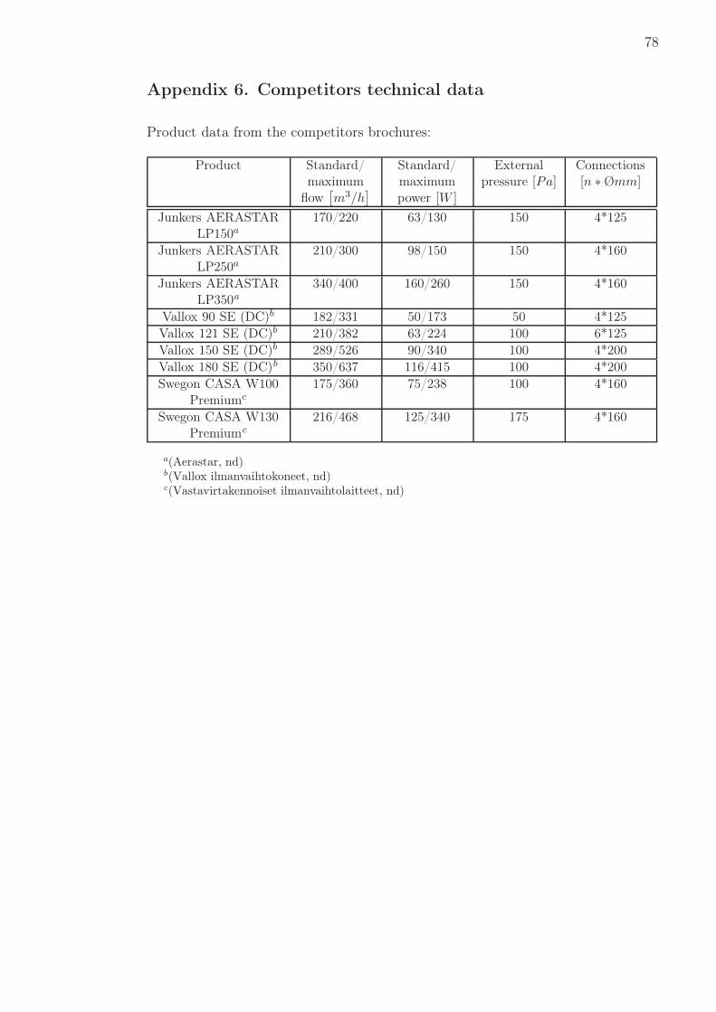
78
Appendix 6. Competitors technical data
Product data from the competitors brochures:
Product Standard/maximum
flow[
m3/h]
Standard/maximumpower [W ]
Externalpressure [Pa]
Connections[n ∗ Ømm]
Junkers AERASTARLP150a
170/220 63/130 150 4*125
Junkers AERASTARLP250a
210/300 98/150 150 4*160
Junkers AERASTARLP350a
340/400 160/260 150 4*160
Vallox 90 SE (DC)b 182/331 50/173 50 4*125
Vallox 121 SE (DC)b 210/382 63/224 100 6*125
Vallox 150 SE (DC)b 289/526 90/340 100 4*200
Vallox 180 SE (DC)b 350/637 116/415 100 4*200
Swegon CASA W100Premiumc
175/360 75/238 100 4*160
Swegon CASA W130Premiumc
216/468 125/340 175 4*160
a(Aerastar, nd)b(Vallox ilmanvaihtokoneet, nd)c(Vastavirtakennoiset ilmanvaihtolaitteet, nd)

79
Appendix 7. RadiCal fans
[Material deleted due to confidentiality]

80
Fan curves of the RadiCal fan R3G190RG2303 (Weinmann, 2011).
pres
sure
,p
[Pa]
1
2
3
4
5
6
7
8
9
10
1112
14
1516
volumetric flow, Q [m3
h]
Measured values of the RadiCal fan R3G190RG2303 in operating points (Wein-
mann, 2011).
# U [V ] f [Hz] n[
1
min
]
P [W ] I [A] Lp [dB(A)] Q[
m3
h
]
p [Pa]
1 230 50 3520 88 0,63 70 755 02 230 50 3470 93 0,67 63 645 2003 230 50 3375 96 0,80 58 450 4004 230 50 3445 94 0,68 63 295 5005 230 50 3000 55 0,39 66 645 06 230 50 3000 60 0,43 59 560 1507 230 50 3000 68 0,49 55 400 3128 230 50 3000 62 0,45 60 260 3809 230 50 2400 28 0,20 62 515 010 230 50 2400 31 0,22 55 445 9611 230 50 2400 35 0,25 50 320 20012 230 50 2400 32 0,23 55 205 24413 230 50 1800 12 0,08 55 385 014 230 50 1800 13 0,09 48 335 5415 230 50 1800 15 0,11 44 240 11216 230 50 1800 13 0,10 49 155 137
Reached efficiency with the RadiCal fans:
[Material deleted due to confidentiality]

81
Appendix 8. Beam torque optimization
[Material deleted due to confidentiality]

82
[Material deleted due to confidentiality]

83
Appendix 9. Beam thickness optimization
[Material deleted due to confidentiality]

84
[Material deleted due to confidentiality]

85
Appendix 10. Pressure drop in fibrous filters
0
20
40
60
80
100
120
140
0 0,10 0,20 0,30 0,40 0,50
F9 F8F7
M6
M5
G4
G3
G2
G1
pre
ssure
dro
p,∆
p[P
a]
mean facing velocity ufacing[m/s]
Pressure drop in fibrous filters as a function of mean facing velocity. Filtersare classified and values are calculated according to the requirements given instandard DIN 779.
In the filter calculations, the equations are given by (Ensor and Donovan, 1988):
αfilter =the solidity of the filter, normally in fibrous filters 5 − 6 %
dparticle =the diameter of the particle wanted to be filtered, 0,4 µm (DIN EN 779,
2009, p. 12)
dfiber =the diameter of a single fiber, in fine glass fiber filters 0,5 − 5 µm
Zfilter =the thickness of the filter, 0,30 − 0,75 mm according to the filter manu-
facturers
ufacing =the mean facing velocity between air flow and filter
Efficiency of a single fiber is given by:
ηfiber = ηd + ηd,i + ηi
Effect of the diffusion is given by:
ηd = 2,9 ∗ Ku− 1
3 ∗ Pe−2
3 + 0,624Pe
Where the Kuwabara number is:
Ku = −0,75 − 12∗ ln αfilter + αfilter − 0,25 ∗ α2
filter
And the Peclet number is:
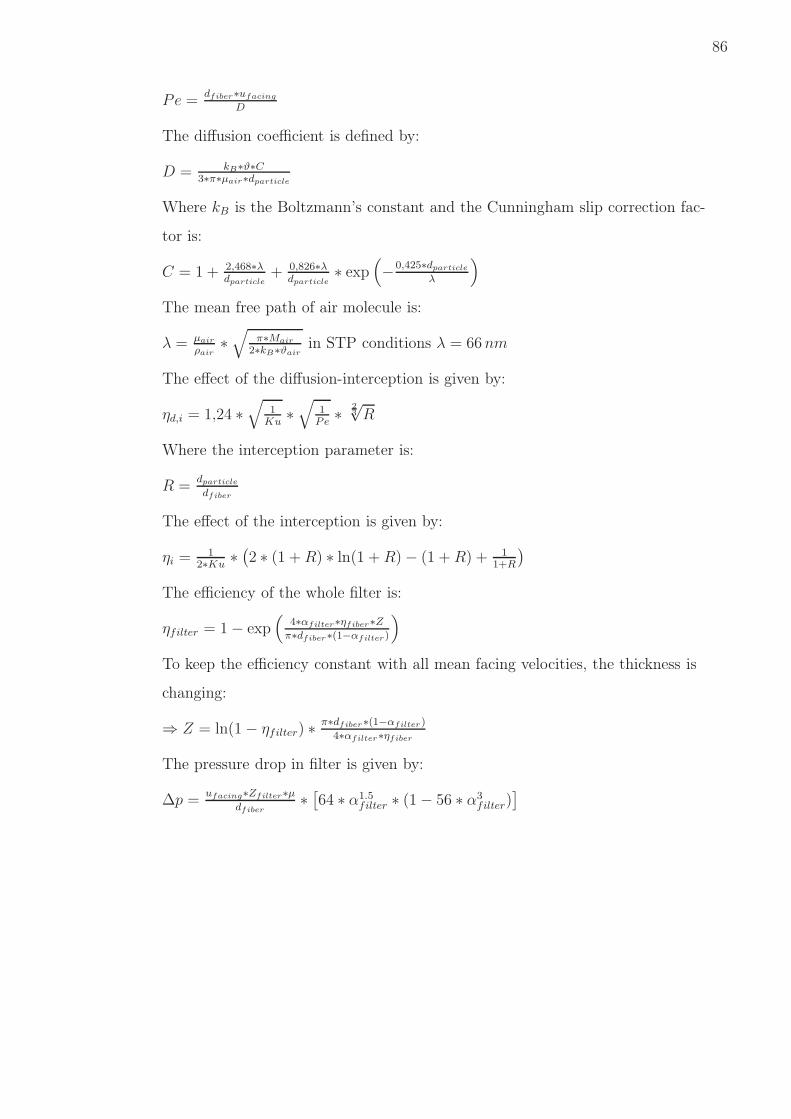
86
Pe =dfiber∗ufacing
D
The diffusion coefficient is defined by:
D = kB∗ϑ∗C3∗π∗µair∗dparticle
Where kB is the Boltzmann’s constant and the Cunningham slip correction fac-
tor is:
C = 1 + 2,468∗λdparticle
+ 0,826∗λdparticle
∗ exp(
−0,425∗dparticle
λ
)
The mean free path of air molecule is:
λ = µair
ρair∗
√
π∗Mair
2∗kB∗ϑairin STP conditions λ = 66 nm
The effect of the diffusion-interception is given by:
ηd,i = 1,24 ∗√
1Ku
∗√
1Pe
∗23
√R
Where the interception parameter is:
R =dparticle
dfiber
The effect of the interception is given by:
ηi = 12∗Ku
∗(
2 ∗ (1 + R) ∗ ln(1 + R) − (1 + R) + 11+R
)
The efficiency of the whole filter is:
ηfilter = 1 − exp(
4∗αfilter∗ηfiber∗Z
π∗dfiber∗(1−αfilter)
)
To keep the efficiency constant with all mean facing velocities, the thickness is
changing:
⇒ Z = ln(1 − ηfilter) ∗π∗dfiber∗(1−αfilter)
4∗αfilter∗ηfiber
The pressure drop in filter is given by:
∆p =ufacing∗Zfilter∗µ
dfiber∗
[
64 ∗ α1.5filter ∗ (1 − 56 ∗ α3
filter)]

87
Appendix 11. Water cycles
[Material deleted due to confidentiality]

88
[Material deleted due to confidentiality]

89
Appendix 12. Pressure loss in cooling box
[Material deleted due to confidentiality]

90
Appendix 13. Pressure loss in third construction
[Material deleted due to confidentiality]

91
[Material deleted due to confidentiality]

92
[Material deleted due to confidentiality]
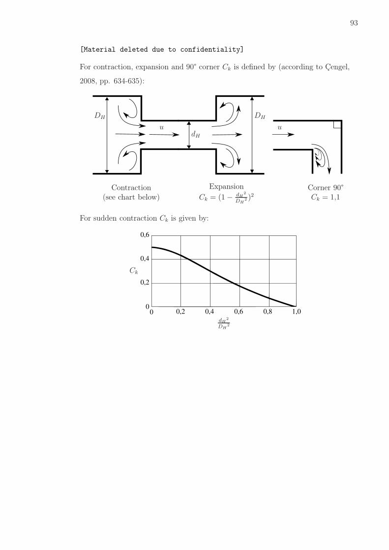
93
[Material deleted due to confidentiality]
For contraction, expansion and 90° corner Ck is defined by (according to Çengel,
2008, pp. 634-635):
uu
DHDH
dH
Contraction(see chart below)
Expansion
Ck = (1 − dH2
DH2 )2
Corner 90°Ck = 1,1
For sudden contraction Ck is given by:
0 0,2 0,4 0,6 0,8 1,00
0,2
0,4
0,6
Ck
dH2
DH2

94
Appendix 14. Computational pressure loss
[Material deleted due to confidentiality]

95
[Material deleted due to confidentiality]