Embed Size (px)
Citation preview

DEPARTMENT OF COMPUTER SCIENCE AND ENGINEERING
MITRA DEHGHANI
DESCRIPTIVE DATA MINING APPROACH TO
VISUALIZE DIABETES BEHAVIOUR
Master’s Thesis
Degree Programme in Computer Science and Engineering
May 2014

Dehghani M. (2014) Descriptive Data Mining Approach to Visualize Diabetes
Behaviour. University of Oulu, Department of Computer Science and Engineering.
Master’s Thesis, 50 p.
ABSTRACT
Diabetes mellitus is a chronic disease that imposes unacceptably high human, social
and economic costs on all countries. Moreover, minimizing its incidence and
prevalence rate as well as its costly and dangerous complications requires effective
management. Diabetes management hinges on close cooperation between the
patient and health care professionals. However, owing to the increasing prevalence
of diabetes, one emerging global trend is to replace traditional face-to-face health
care with remote patient monitoring by taking advantage of new advances in
electronics, such as wireless sensor networks and body sensors. This significantly
reduces the cost and service pressures that health centers are facing, but produces
a huge amount of heterogeneous data, confronting us with new challenges related
to ‘big data’. One established method of handling the big data challenge is data
mining.
Data mining provides a variety of techniques to analyze big data in order to
discover hidden knowledge. This study is an effort to design and implement a
descriptive data mining approach and to devise association rules to visualize
diabetes behaviour in combination with specific life style parameters, including
physical activity and emotional states, particularly in elderly diabetics. The main
goal of this type of data mining is to discover critical time stamps and salient
parameters that lead patients either to success or failure in diabetes self-care. The
visualization method is aimed at creating sufficient motivation in patients to
improve their self-care through life style changes. At the same time, it provides a
decision support system for health care professionals to improve diabetes
treatment.
Key words: Diabetes, big data, data mining, blood glucose, physical activity,
emotional state.

Dehghani M. (2014) Deskriptiivinen tiedonrikastus diabeteksen käyttäytymisen
visualisointia varten. Oulun yliopisto, Tietotekniikan osasto. Diplomityö, 50 p.
TIIVISTELMÄ
Diabetes mellitus, joka aiheuttaa inhimillistä, sosiaalista ja taloudellista haittaa
globaalisti, vaatii sairauden tehokasta hallintaa vaarallisten komplikaatioiden
esiintymisriskin pienentämiseksi. Sairauden hallinta/hoito vaatii läheistä
yhteistyötä potilaan ja hoitohenkilökunnan välillä. Koska taudin esiintymistiheys
on kasvava, useat maat pyrkivät siirtymään kontaktihoidosta etämonitorointiin
käyttämällä hyväksi uusia elektronisia sovelluksia kuten langattomia
anturiverkkoja ja kehon antureita. Tämä vähentäisi merkittävästi
terveyskeskusten kuormitusta, mutta tuottaisi suuria määriä heterogeenista dataa,
jonka asettaa uusia haasteita.
Tiedonrikastus, tarjoaa useita tekniikoita piilossa olevan tiedon tutkimiseen.
Tässä diplomityössä suunnitellaan ja toteutetaan deskriptiivinen
tiedonrikastuslähestymistapa ja assosiaatiosäännöt visualisoimaan diabeteksen
käyttäytymistä yhdistämällä elintapaparametreja mukaan lukien diabeetikoiden
fyysinen aktiivisuus ja mieliala. Tiedonrikastuksen päämääränä on tutkia kriittiset
ajoitukset ja tärkeimmät parametrit, jotka johtavat diabeteksen omahoidon
tasapainoon tai epätasapainoon. Visualisointitavan on tarkoitus luoda tarpeeksi
motivaatiota potilaalle parantamaan heidän sairautensa hoitotasapainoa
muuttamalla elintapoja kuten myös antamalla tukea terveydenhuollon
päätöksenteolle hoidon parantamiseksi.
Avainsanat: Diabetes, big data, tiedonrikastus, verensokeri, fyysinen aktiivisuus,
mieliala.

TABLE OF CONTENTS
ABSTRACT .................................................................................................. 2
TIIVISTELMÄ ............................................................................................. 3
TABLE OF CONTENTS ............................................................................ 4
FORWARD ................................................................................................... 6
LIST OF ABBREVIATIONS AND SYMBOLS ....................................... 7
1. INTRODUCTION ................................................................................. 9
2. BACKGROUND .................................................................................. 10
2.1. Diabetes mellitus ...........................................................................................................10
2.2. Diabetes in Elderly ........................................................................................................11
2.3. Diabetes management ...................................................................................................12
2.4. Data mining...................................................................................................................13
2.5. Big data mining challenges ...........................................................................................14
2.6. Big data mining in health care ......................................................................................15
3. METHODS AND MATERIALS ........................................................ 17
3.1. Data collection ..............................................................................................................17
3.2. Data preparation ............................................................................................................18
3.3. Data analysis and visualization .....................................................................................18
3.4. Population statistics ......................................................................................................23
4. DATA ANALYSIS ............................................................................... 24
4.1. Customer level implementation ....................................................................................24
4.1.1. Data preparation ................................................................................................. 24
4.1.2. Primary variable-based data analysis ................................................................. 24
4.1.3. Secondary variables-based data analysis ............................................................ 29
4.1.4. Data correlation .................................................................................................. 31
4.2. Overall level implementation ........................................................................................40
4.2.1. Data distribution analysis .................................................................................... 40
4.2.2. Rate of success analysis ....................................................................................... 42
4.2.3. Weekdays and daily time stamps analysis............................................................ 43
4.2.4. Primary and Secondary variables-based analysis ............................................... 44
5. DISCUSSION ....................................................................................... 46
6. SUMMARY .......................................................................................... 48
7. REFERENCES..................................................................................... 49

FORWARD
As my thesis work I had honor to participate in SIMSALA project by University of
Oulu, Optoelectronics and Measurements Techniques Laboratory. I would like to
express my deepest appreciation to all those who provided me the possibility to
complete this thesis especially my supervisor Prof. Esko Alasaarela for his
encouragements and superb guidance as well as Prof. Tapio Seppänen for his valuable
hints and comments.
I am grateful to the OEM laboratory especially Dr. Matti Kinnunen for giving me the
opportunity and providing necessary tools and fund for conducting this research. I also
would like to thanks project team members Dr. Hannu Sorvoja, Dr. Timo Takala and
Mrs. Eija Vieri whose suggestions and experiences helped me to improve my work.
I’d also like to thank my friends Justice Akanegbu, Fardis Khademolhoseini and
Jonathon Kisner who paid their valuable time for reading and correcting my English.
At the end I would like to express appreciation to my beloved husband Ali who was
always my support in the moments when there was no one to answer my queries. I also
thank my wonderful children Raha and Sepehr for always making me smile and for
understanding on those times when I was writing my thesis instead of playing games.
Mitra Dehghani
Oulu, March 10th 2014
LIST OF ABBREVIATIONS AND SYMBOLS
AFB After Breakfast
AFD After Dinner
AFL After Lunch
AM Ante Meridiem (the time before noon)
Apr April
BFB Before Breakfast
BFD Before Dinner
BFL Before Lunch
BG Blood Glucose
CORRCOEF Correlation Coefficient
DSCS Diabetes Self-care Support
DEHKO Development Programme for the Prevention and Care of Diabetes
DogIMU Movement sensor by Domuset Ltd
e-Health Electronic Health (Internet-based Health)
IDF International Diabetes Federation
KELA Kansaneläkelaitos (Social Insurance Institution of Finland)
LADA Latent Autoimmune Diabetes in Adults
Matlab Math works Laboratory Software
NAN Not a Number
OEM Optoelectronics and Measurements Techniques
PM Post Meridiem (the time after noon)
Sensorfit Mobile application by Sensorfit Ltd.
SIMSALA Senior Citizens Integrated Multi-sensor Security and Care Solutions
Three V’s Voluminous, Variety and Velocity
TS Time Stamp
V3 Voluminous, Variety and Velocity
mmol/L Millimoles per Litre
𝑛 Number of measurements
𝑝 Pearson product-moment correlation coefficient
𝑟 Correlation
𝑥 Random variable standing for a measurement
𝑥𝑖 i th element in measurements 𝑥
�̅� Sample mean of measurements x
𝑦 Random variable standing for a measurement
𝑦𝑖 i th element in measurements 𝑦
�̅� Sample mean of measurements y
Δt Time delay

9
1. INTRODUCTION
Data mining with extremely intensive and extensive applications in many organizations
is becoming increasingly popular and even essential in healthcare. Data mining
applications can greatly benefit all parties involved in the healthcare industry. It can be
used by; healthcare insurers to detect fraud and abuse, healthcare organizations to make
customer relationship management decisions, physicians to identify effective treatments
and patients to receive better and more affordable healthcare services. Data mining
provides methodology and technology to process and analyze huge amounts of data into
useful information for decision making that is a fundamental part of healthcare
management. Taking advantage of recent advances in electronics and communication
services such as wireless sensor networks, enhances this management by enabling
remote monitoring provided by real time data acquisition and on time decision making.
This remote monitoring is critical and vital in healthcare services, especially for groups
such as elderly who lives alone and diabetics who don’t need to be hospitalized and their
disease is mainly controlled by themselves. The cost of traditional face-to-face
healthcare services along with considerable population of such groups, especially in
some societies like Finland, emphasizes the importance and necessity of healthcare
remote services. This study is an effort to visualize the results of data mining on data
obtained from SIMSALA (Senior Citizens Integrated Multi-sensor Security and Care
Solutions) research project which is a multi-sensor integrated system for elderly health
and safety monitoring by the university of Oulu. Volumes of data, variety of their time
bases from daily to minutely along with its complexity due to different types of signals
and data are the main challenges in this study. Additionally, the results must be reported
in a way that can create enough motivation in the patient to improve his self-care; and
can be applicable as a decision support system for physician and health centers in
diabetes treatment and management. In the following chapter, after a review on diabetes
and diabetics, main challenges in its management, especially in elderly, along with
recent researches and methodologies to improve its management are discussed. In
chapter three and four the methodology of data mining and its implementation are
explained. In chapter five the results of data analysis along with its success in achieving
desired objectives of SIMSALA’s project are discussed. In chapter six, a summary of
study as well as its strength and weakness points, its limitations and future applications
are provided.

10
2. BACKGROUND
Diabetes is one of the most common non-communicable diseases around the world. It is
estimated to be the fourth or fifth reason for death in most high-income countries.
Diabetes is nominated by IDF (International Diabetes Federation) as one of the most
challenging health issues of 21st century [1]. In this chapter after a review on diabetes
and diabetics, main challenges in its management especially in elderly along with recent
researches and the methodologies to improve its management are discussed.
2.1. Diabetes mellitus
Diabetes is a chronic disease that occurs when the body cannot produce enough insulin
or cannot use it effectively which results in BG (Blood Glucose) not to be absorbed
properly by the body cells and remains circulating in the blood [1].
There are three types of diabetes:
- Type 1 diabetes;
- Type 2 diabetes,
- Gestational diabetes
Type 1 diabetes encompasses diabetes that is primarily a result of pancreatic beta cell
destruction that leads to not enough production of insulin. This type can affect any age
but usually occurs in children and young adults. These diabetics can lead a normal life
through combination of a daily insulin therapy, healthy diet, close monitoring and
regular physical exercise [2].
Type 2 diabetes is the most common one that usually occurs in adults but is
increasingly seen in children and adolescents, too. This type is also known as an insulin
resistance because, in this type the body can produce insulin but either it is not sufficient
or the body cannot respond to its effect leading glucose remains circulating in blood.
This type also includes LADA (Latent Autoimmune Diabetes in Adults), describing a
small number of people with diabetes type 2 who appear to have an immune-mediated
loss of pancreatic beta cells [3]. Many type 2 diabetics can control their BG level
through a healthy diet and an increased physical activity or oral medication.
Gestational diabetes mellitus refers to a glucose intolerance with onset or first
recognition during pregnancy due to poorly managed BG. This group must be closely
monitored to control their BG level and minimize the risk for the baby. This can be done
by healthy diet, moderate exercise and sometimes insulin therapy or oral medication [2].
Poorly managed BG in diabetics can lead to one of the critical disease situations
called hyperglycemia and hypoglycemia due to an extremely high or low BG level. Such
situations must be detected and treated as soon as possible to prevent diabetic coma [4].
Based on classification shown in Table 1 diabetics must control their BG level in safe
level between upper and lower limit of normal level diagnosed by their physician.

11
Table 1. Categorization of BG level in diabetics
Hypoglycemia Low
level
Lower
limit of
Normal
Normal
level
Higher
limit of
Normal
High
level Hyperglycemia
BG (mmol/L) <=3 3-4 4-4.4 4.4-6 6-11 11-15 >=15
Besides BG there are some other important factors that must be monitored regularly in
diabetes care such as blood pressure, weight, emotional states, physical activity and
calories consumption.
Blood pressure must be controlled in diabetics because hypertension is more prevalent
in them. Early diagnosis and effective management of hypertension is paramount in the
diabetes care [5].
Another important factor in diabetes care is weight control. Losing a few pounds can
decrease their BG level along with reducing the risk for high blood pressure and heart
diseases. The reason is the effect of body fat on insulin resistance. Too much body fat
decreases the body’s ability to use the insulin. Weight loss helps insulin resistance that
allows the body to use the insulin that improves BG control [6].
The stress of managing diabetes every day and its effect on the brain can lead
diabetics to some challenging mental diseases such as depression. Studies show a link
between them but it is not approved yet that such feelings can increase the risk of
diabetes or diabetes increases their frequencies [7]. So as an important factor diabetics
daily emotional states can be assessed for example by using psychological
questionnaires.
Physical activity is defined as any bodily movement produced by skeletal muscles that
require energy expenditure. Regarding to this definition, lack of physical activity has
been identified as the fourth leading risk factor for global mortality and estimating the
main cause for approximately 27% of diabetics. Studies show that regular and adequate
level of physical activities reduces the risk of diabetes along with improving its care by
reducing the risk of hypertension, increasing calories consumption and weight control
[8].
2.2. Diabetes in Elderly
The definition of elderly varies although it is generally agreed as a concept referring to a
person with age 60 and over who is characterized by a slow, progressive frailty which
continues to the end of life [9]. Population aging has an increasing trend around the
world in a way that the global share of elderly from 9.2 percent in 1992 reached to 11.7
percent in 2013 and is estimated to reach 21.1 percent by 2050. As aging population
increases, the reasons for death and disabilities are changing from infectious to non-
communicable diseases such as diabetes [10].

12
The prevalence of diabetes increases with aging. Studies show that 10% of population
over 60 of age and 16% to 20% over 80 of age, have diabetes. In addition to
considerable elderly diabetics population, the importance of early diabetes diagnosis and
management increases in elderly due to their increasing potential for premature death,
functional disability and coexisting illnesses such as hypertension and stroke. They are
also at greater risk for several common geriatric syndromes such as depression,
cognitive impairment, urinary incontinence, injurious falls, and persistent pain [11].
These conditions increase the complexity of diabetes management in elderly.
Lifestyle interventions including nutrition therapy and exercise, is one of the best
known ways for diabetes prevention and management in elderly.
2.3. Diabetes management
Diabetes is a chronic illness that requires continuous medical care along with the patient
self-care to prevent acute complications and to reduce the risk of long-term
complications.
Diabetics population is increasing around the world within all age groups. The IDF
states that every ten seconds, two people are diagnosed with diabetes. Their increasing
trend leads to an increase from their 30 million population in 1985 to 150 million people
in 2000 and is projected to rise further to 380 million by 2025 [12].
Different regions around the world are affected by diabetes prevalence in significant
different degrees. Among 138 million 20-79 years old diabetics in 2013, Western pacific
has the most people with diabetics and Africa has the least [1]. Based on statistics from
Kela (Social Insurance Institution of Finland), number of people with diabetes in Finland
was 195500 persons in 2000, 220000 in 2003 and is projected to rise to half a million by
2030. Regards to different types of diabetes distribution, Finland is known as a special
case in type 1 with the highest rate of incidence in the world [13].
In addition to diabetics population, diabetics special health care requirements impacts
significant costs for societies. Among adults aged 20 to 49 years, those with diabetes
were two times more likely to see a family physician and two to three times more likely
to see a specialist. Also, people with diabetes were 3 times more likely to require
hospital admission with longer lengths of stay [14]. Based on statistics provided by IDF,
global health expenditure due to diabetes was 548 billion US dollars and is predicted to
rise to 627 billion US dollars by 2035 [1]. Based on studies by DEHKO (Development
Programme for the Prevention and Care of Diabetes), the costs for diabetes in Finland
constitute 12% of Finland health care expenditure. As estimated, 90% of the costs
caused by diabetics arise from treatment for complications such as eyes, kidneys, feet
and heart damages [13]. These statistics approve the importance and necessity of
effective diabetes management in order to prevent such costly and dangerous
complications.
Effective management of diabetes requires close cooperation between the person with
diabetes and health professionals. In other hand by taking advantages of new advances
in electronics such as wireless sensor networks and body sensors, societies try to replace

13
traditional face to face health care with remote patient monitoring in order to reduce
such costs and service pressures from health centers.
The inputs of diabetes management system can be patient’s daily measurements from
BG levels, blood pressure, diet, exercise, etc. to foot image. The output should
represents the diabetes behaviour providing a feedback to the patient about his
success/failure in diabetes self-care and additionally being served as a decision support
system by health professionals to improve diabetes treatment. More input measurements
enriches diabetes management and enables it to reveal critical factors in patient’s self-
care success/failure. But making a variety of daily measurements for a period as long as
life time increases the complexity of self-care especially in elderly. Taking advantages
of sensors that do measurements automatically facilitates these measurements and
consequently improves the efficiency of self-care.
SIMSALA project is an example of such Multi-sensor integrated system for elderly
health and safety monitoring by University of Oulu. The purpose is to raise the quality
of home care that seniors receive and to improve their safety at home. In this project by
using wireless sensor networks, some vital physiological signs such as BG level, blood
pressure, weight scale, physical activity, calories consumption and emotional states are
monitored from home. As last phase of this project, this study by aims of data mining
approaches tries to visualize the results and benefits of this project as a decision support
system to facilitate and improve diabetes care in elderly.
2.4. Data mining
Data mining is defined as the process of analyzing data from different perspectives in
order to find unknown trends and patterns in them and converting them to useful
information. Data mining is not a new idea, it has been widely used by financial
institutions for credit scoring, fraud detection, etc.; marketers for direct marketing and
cross-selling; manufacturers for quality control and maintenance schedule; as well as
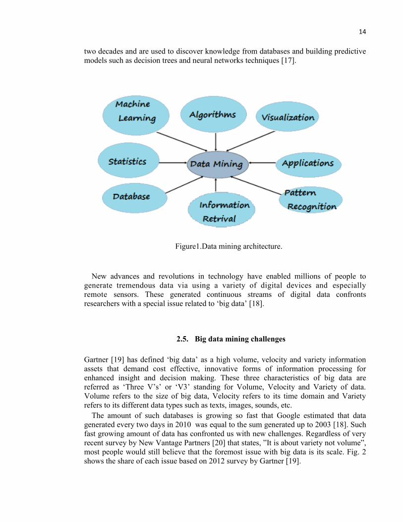
hospitals [15]. Data mining architecture is shown in Fig. 1.
The most common types of data mining analysis are Descriptive and Predictive
modeling which are used to discover patterns and rules. Descriptive modeling is used to
collectively describe all of the data in a given data set. Specifically, this approach
synthesizes all of the data to provide information regarding trends, segments and clusters
that are present in the information searched. For example, the trends of BG level in a
diabetic. Predictive modeling is used for prediction of another variable that is relevant to
the data reviewed. For example, to predict diabetes behaviour due to increasing physical
activity. Association rules that aims to extract important correlation between data items
is a descriptive data mining task [16].
There are a variety of data mining techniques and tools that can be classified into
classical techniques and next generation techniques. Classical techniques use statistical
tools and concerns the collection and description of data such as histograms, linear
regression, nearest neighbor, etc. The next generation techniques were developed in last
14
two decades and are used to discover knowledge from databases and building predictive
models such as decision trees and neural networks techniques [17].
Figure1.Data mining architecture.
New advances and revolutions in technology have enabled millions of people to
generate tremendous data via using a variety of digital devices and especially
remote sensors. These generated continuous streams of digital data confronts
researchers with a special issue related to ‘big data’ [18].
2.5. Big data mining challenges
Gartner [19] has defined ‘big data’ as a high volume, velocity and variety information
assets that demand cost effective, innovative forms of information processing for
enhanced insight and decision making. These three characteristics of big data are
referred as ‘Three V’s’ or ‘V3’ standing for Volume, Velocity and Variety of data.
Volume refers to the size of big data, Velocity refers to its time domain and Variety
refers to its different data types such as texts, images, sounds, etc.
The amount of such databases is growing so fast that Google estimated that data
generated every two days in 2010 was equal to the sum generated up to 2003 [18]. Such
fast growing amount of data has confronted us with new challenges. Regardless of very
recent survey by New Vantage Partners [20] that states, ”It is about variety not volume”,
most people would still believe that the foremost issue with big data is its scale. Fig. 2
shows the share of each issue based on 2012 survey by Gartner [19].

15
Figure 2.The share of Three V’s in big data mining.
Additionally big data is becoming a mature discipline. Based on 2013 survey [20],
90% of surveyed organizations are dealing with big data. Regarding to such popularity
along with special challenges related to big data characteristics, emphasizes are laid on
the necessity of suitable data management and analytics activities to discover their
hidden knowledge.
Comparing with the results from mining the conventional datasets, analyzing
voluminous interconnected heterogeneous big data gives us the opportunity to maximize
our knowledge and provide more effective decision support system for organizations. To
attain this goal, big data mining must exploit massively parallel computing architectures
enabling it to deal with heterogeneity, extreme scale, velocity, privacy, accuracy, trust
and intra-activeness at the same time that is beyond the capability of existing mining
techniques and algorithms [18].
Big data mining is a promising research area still in its infancy and much work is
required to overcome its challenges.
2.6. Big data mining in health care
Nowadays the huge amount of heterogeneous data generated by health care
organizations provides a vast potential for data mining applications in health care. These
applications can greatly benefit all parties involved in this industry. For example, it can
be used by healthcare insurers to detect fraud and abuse, healthcare organizations to
make customer relationship management decisions, physicians to identify effective
treatments and patients to receive better and more affordable healthcare services. Data

16
mining provides methodology and technology to process and analyze huge amounts of
data into useful information to facilitate, improve and speed up decision making process
in medical domain [15].
Diabetes is a particularly opportune disease for data mining because:
- Many diabetic databases with historic patient information are available;
- Diabetes is a disease with categorized treatment patterns,
- Its applications in pattern recognition enables physician to predict diabetes
terrible afflictions such as blindness, kidney failure and heart failure that results
in increased treatment efficiency and decreased costs [21];
Data mining can provide a variety of applications in diabetes management which
include: diabetes diagnosis [23,24,26], preventing diabetes via analysis of its risk
factors [25,26], genomic data analysis to discover candidates genes related to diabetes
[24], prediction of diabetes behaviour as well as its dramatic complications [24],
assessment of diabetes management [26] and monitoring diabetes behaviour [27,29].
All these studies approve that data mining can significantly help diabetes research and
ultimately improve the quality of health care in diabetics. In this study a descriptive data
mining model for elderly diabetics care is designed and implemented. The main goal of
the study is to visualize diabetes behaviour in these patients. The discovered knowledge
reveals most important factors affecting their diabetes self-care and provides a decision
support systems for physicians and health centers to improve their quality of treatment.
Unlike previous studies in which diet and medications (oral and injections) as primary
diabetes treatment tools have important roles to reasoning diabetes behaviour [21], in
this study we just analyze influential parameters including physical activity, calories
consumption, weight scale and emotional states to discover the most important factors in
diabetes care in the patients under study. Considering diabetes as a disease of ‘numbers’,
by limiting measurements to just influential factors along with taking advantages of
wireless sensor networks that enables patients to register measurements automatically,
we try to minimize patient’s involvement in data production. This benefits especially
elderly whose ability and patience in daily measurements and registrations is considered
as a big challenge for their effective self-care.

17
3. METHODS AND MATERIALS
In this chapter, the methodologies for data collection and measurement in previous
phases in SIMSALA project are briefly described. As the main goal of this thesis, the
methodology for descriptive data mining including data preparation, data analysis and
visualization its results regarding to its application in diabetes management and diabetes
self-care are explained in detail. Population statistics of data obtained from SIMSALA
project which is the material for this study are summarized at the end of this chapter.
3.1. Data collection
The multi-sensor integrated system that is designed in SIMSALA project [29] is used to
collect data such as BG, blood pressure, daily physical activity and calories
consumption, weight and emotional states from the patients who participated in this
study.
- Bluetooth enabled glucose meter was used to measure and transfer BG data to
the server. Diabetics should do BG measurements in six daily time stamps BFB
(Before Breakfast), AFB (After Breakfast), BFL (Before Lunch), AFL (After
Lunch), BFD (Before Dinner) and AFD (After Dinner).
- Daily systolic and diastolic blood pressure data was measured and transferred to
the server using Bluetooth enabled blood pressure meter.
- Patient’s physical activity was measured using DogIMU movement sensor or
Sensorfit mobile application. Both sensors can automatically acquire acceleration
data from the body and store it in the server database for further use such as
calculating daily calories consumption as well as fall detection in patients [30].
Sensorfit categorizes the measurements in five activity levels including ‘passive’,
‘low’, ‘medium’, ‘high’ and ‘very high’ levels.
- Wireless Bluetooth weight scale was used to measure and transfer daily weight
measurement to the server.
- ZEF online questionnaire was used to measure and quantified patient’s feelings
in the morning and evening as his daily emotional states for five aspects
including loneliness, pain, mood, appetite and overall daily feelings. The results
were categorized in five levels including: very bad (0-20), bad (20-40),
indifferent (40-60), good (60-80) and very good (80-100).
18
3.2. Data preparation
Importing recorded data from SIMSALA database in text format to Matlab (Math works
Laboratory Software) is the first step in data preparation.
Since the main goal of SIMSALA project is concerned with diabetics, BG data is
considered as primary data. Then other data are prepared along with it as secondary data.
So other data beyond BG time domain is neglected in the analysis step.
In diabetes care, blood samples must be examined before each meal and one or two
hours after meal. This is considered as six time stamps per day. By default, these six
time stamps are assumed as 6, 9 and 11AM, 2, 5 and 8PM. Then each measured BG
level assigns to the closest time stamp. This assignment was done to facilitate following
steps for analysis and visualization of diabetes behaviour.
The same preparation procedure is done on systolic and diastolic blood pressure
measurements in the time domain limited by BG measurements.
Daily physical activity in different levels that have been averaged in each half an hour
are used as the basis for patient activity and calories consumption. Each level of activity
has a constant coefficient in calories consumption. As the coefficients, which are used
by Sensorfit application are unknown, an estimation is used instead. By using some
records of patients in which activity in all levels existed and resulted to catch their goal
in daily calories consumption, these coefficients are estimated by Problem Solver in
Microsoft Excel. Equation (1) shows this estimation.
Activity at time t=activity level 1 * 0.42 + activity level 2 * 1 + activity level 3 * 3.37 +
activity level 4 * 5.97 + activity level 5 * 6.01 (1)
Where activity level 1 to 5 are ‘passive’, ‘low’, ‘medium’, ‘high’ and ‘very high’ activity
measurements.
Daily calories consumption, weight measurements and feelings data are prepared just
by time domain limitation by the time domain of BG measurements.
3.3. Data analysis and visualization
In diabetes control, daily diet and injected insulin doses are known as the main important
factors while other factors such as daily activity and feeling are considered as minor.
however, in this study, data from insulin injection and daily diet were not available, so
we try to reveal how patient’s life style from these two aspects affected patient’s
diabetes self-care.
The frequency analysis provides statistics and graphical displays that are useful to
start looking at measured data. Providing frequency reports, histograms and bar charts
helps in visualizing how data are distributed in different categories such as :

19
- Distribution of BG data in each defined range (Hyperglycemia, High level, Higher
limit of Normal, Normal ,Lower limit of Normal, Low level and Hypoglycemia
ranges) as shown in Fig. 3;
Figure 3.BG distribution in different ranges.
- Distribution of BG data in each defined time stamp (BFB/AFB, BFL/AFL and
BFD/AFD ) as shown in Fig. 4;
Figure 4.BG distribution in different daily time stamp.

20
- Distribution of BG data in each day of week as shown in Fig. 5;
Figure 5.BG distribution in different weekdays.
- Distribution of blood pressure data in each defined range (Normal, High and
Hypertension grade 1/2/3 levels) as shown in Fig. 6;
Figure 6.Blood pressure distribution.
- Distribution of average physical activity in each time stamp and each day of week as
shown in Fig. 7 for Fridays;

21
Figure 7.Physical activity distribution in Fridays.
- Distribution of calories consumption in each day of week as shown in Fig. 8,
Figure 8.Distribution of calories consumption.
- Distribution of feelings at morning and evening in each day of week.
Joint frequency reports visualizes how well data are distributed in each joint category.
For example distribution of BG data in each time stamps of each day of week helps to
clarify the points in which patients met failures in their diabetes control. An in-depth
detail of such joint frequency reports are explained in chapter four. Comparing
distribution of different variables (BG, blood pressure, activity, calories consumption
and feelings) at such points, provides some reasons for these failures. For example, what
was patient’s feeling or physical activity in such points? One statistics that helps doing
this comparison is data correlation analysis.
We assumed that each patient follows her diabetics daily diet and doses of insulin
injection as prescribed and experienced. Then by calculating the correlation between
patient’s self-care outcomes, we try to reveal the most significant factors resulting in

22
patient’s success or failure in his disease control. In this analysis, Pearson’s correlation
coefficient in Equation (2) is used to calculate the linear dependency between desired
variables.
𝑟 =∑ (𝑥𝑖−�̅�)(𝑦𝑖−�̅�)𝑛
𝑖=1
√∑ (𝑥𝑖−�̅�)2√∑ (𝑦𝑖−�̅�)2𝑛𝑖=1
𝑛𝑖=1
(2)
Where 𝑟 is correlation between 𝑥 and 𝑦 with mean �̅� and �̅� .
In Matlab, CORRCOEF is the function that calculates this correlation with notation
showed in equation (3).
[ 𝑟 , 𝑝 ] = 𝑐𝑜𝑟𝑟𝑐𝑜𝑒𝑓( 𝑥 , 𝑦 , ′𝑟𝑜𝑤𝑠′ , ′𝑝𝑎𝑖𝑟𝑤𝑖𝑠𝑒′ ) (3)
Where 𝑟 is correlation between 𝑥 and 𝑦 and 𝑝 is correlation coefficient. A significant
correlation exists when 𝑝 is less than 0.05. This correlation is positive if 𝑟 > 0 and is
negative if 𝑟 < 0. Parameter ′𝑝𝑎𝑖𝑟𝑤𝑖𝑠𝑒′ restricts calculation to rows with no NAN
values.
Medical researches approved that physical activity along with patient’s diet and
insulin injection affects patient’s BG level with a time delay Δt. In this research, the
correlation between BG level at time t is analyzed with patient’s physical activity with
decreasing time step size to estimate -time delay- Δt . In this estimation, we used half an
hour step size equal to physical activity measurement’s time intervals.
The dependency between patient’s feeling and BG level is estimated for two daily
feeling’s measurements at morning and evening. We assumed that feeling at morning
affects BG level until 3PM and remaining hours are affected by patient’s feeling in
second half of day that is measured in the evening.
Average value of BG measurements can simply clarify diabetes behaviour in long
term. This value can be averaged separately for each previously defined time stamps or
different weekdays as well as both. If we define the normal range for each patient, the
result curve visualize the points in which BG level exceeds the normal range. The
frequency of the points that fell inside the normal range is defined as the rate of success
in patient’s self-care and for the points outside of normal range as the rate of failure.
In the same way, other curves representing average value of blood pressure, average
value of physical activity in each week day time stamp, average value of goal catch in
daily calories consumption, average value of feelings at morning and evening for
different weekdays are provided.
By comparing provided curves especially in the points where BG exceeds the normal
range, the primary reasons for patient’s success or failure in diabetes self-care can be
apparent. In order to facilitate this comparison, a summary report containing above
curves for each day of week is provided. Additionally, for each specified day, this
summary can be reported. This helps patients and physicians to have an in depth
investigation on days with abnormal value of BG level. A glance on patient’s life style

23
via activity and feeling aspect on previous and following days can reveal more reasons
for this abnormality.
3.4. Population statistics
In this study four diabetics underwent the designed multi-sensor integrated monitoring
system. The population statistics of these patients are summarized in Table 2. Table 3
shows the quantity of data imported from database server for these patients.
Table 2. Population statistics of study
Patient # Age Sex Diabetes type
1 70 Male 2
2 67 Female 2
3 37 Male 1
4 47 Male 1
Table 3. Data quantity
Patient
Number of records
Blood
pressure
Physical
activity
Weight & Calories
consumption
Feeling at
morning
Feeling at
evening
1 112 94 2911 61 77
2 90 34 966 58 51
3 237 28 1000 59 24
4 2185 46 18 2 1
In the following chapter, implementation of described methodology on this data is
explained.

24
4. DATA ANALYSIS
In this chapter the process of data analysis on the patients involved in this study are
discussed. At first the data collected from each patient are prepared, analyzed and
visualized in different reports based on methodology described in chapter three. In order
to clarify this process, methodology implementation is discussed in two levels:
- Customer level in which one patient is chosen and the reports resulting from each
step for this patient as well as correlation between variables in the study are discussed
in detail,
- Overall level in which whole data obtained from all patients will be processed as a
single data and the summary of the result are discussed.
4.1. Customer level implementation
In this level, we chose patient #3 as the customer because in comparison to others he has
less missing data that is necessary to calculate data correlation.
4.1.1. Data preparation
As explained in chapter three, BG is considered as primary variable and others as
secondary. In first step, the data exported from database server in text format must be
imported by Matlab. Regarding to time duration of BG measured data, other data
consisting of blood pressure, physical activity, calories consumption and feelings are
limited to its time duration between Feb. 18th to Apr. 10th. In order to facilitate
correlation calculation, a Total file with records containing each available BG
measurements at time t along with others at the same time, are constructed. This process
especially simplifies time shifting to calculate the most effective time that physical
activity affects BG.
4.1.2. Primary variable-based data analysis
In diabetes management monitoring BG level in long term plays an important role for
patient and physician to assess the disease behaviour. A graph representing average BG
in time domain as well as one that monitor BG measurements distribution in different
levels can meet this necessity. These graphs can be customized to clarify disease
behaviour in specific time stamps and/or in different weekdays. Fig. 9 shows BG
average in different weekdays and different time stamps.

25
The BG level has an average of 9.55 mmol/L with standard deviation of 4.02 which is
shown in Fig. 9 as dotted line and marked as ‘Total_Avg’. Regarding to defined ranges
for BG level in Table 1, average BG level falls within the higher limit of normal range
for this patient. Continuous colored lines in these graphs in Fig. 9, represent BG average
in different weekdays. These lines connect average of BG measurements in different
time stamps that are shown as colored vertical dots.
Taking a glance on these graphs, reveals the points in which the most significant
deviation in BG levels happened. These points can be specified precisely by frequency
analysis of BG data.
Figure 9.BG average in different time stamps of weekdays.
Table 4 shows how BG data are distributed in different level categories from
Hypoglycemia to Hyperglycemia. Fig. 10 provides a graphical demonstration for this
distribution. Using different symbols and colors for different category makes it easier for
patient to realize his disease behaviour.

26
Table 4. Distribution of BG data in different level categories
Hypoglycemia Low
level
Lower
limit of
Normal
Normal
Higher
limit of
normal
High
level Hyperglycemia
Frequency
(%) 0.42 5.91 2.95 13.08 42.19 24.89 10.55
If we consider rate of success in diabetes control when patient can control it in the
range from lower limit of normal to its higher limit, Table 4 specifies this rate for patient
#3 as 58%. The rate of BG in high level is measured as 36% and in low level as 6%.
Figure 10.Distribution of BG data in different level categories.
In Fig. 10 the dashed blue color line shows the average of BG data during
measurement period. the graph clearly shows that this patient has BG mostly in the

27
levels higher than normal. Table 5 and Table 6 show how different level of BG
measurements are distributed in different days of week.
Table 5. Distribution of BG data in different weekdays
Hypoglycemia Low
level
Lower
limit of
Normal
Normal
Higher
limit of
Normal
High
level Hyperglycemia
Monday 0.00 21.43 14.29 6.45 10.00 18.64 20.00
Tuesday 0.00 7.14 0.00 6.45 17.00 27.12 12.00
Wednesday 0.00 21.43 14.29 25.81 21.00 10.17 8.00
Thursday 0.00 21.43 28.57 19.35 18.00 11.86 4.00
Friday 100.00 14.29 28.57 12.90 17.00 5.08 12.00
Saturday 0.00 7.14 0.00 16.13 6.00 13.56 28.00
Sunday 0.00 7.14 14.29 12.0 11.00 13.6 16.00
Table 6. Distribution of BG data in different daily time stamps
Time
stamp Hypoglycemia
Low
level
Lower
limit of
Normal
Normal
Higher
limit of
Normal
High
level Hyperglycemia
TS_1 0.00 7.14 0.00 12.90 21.00 33.90 8.00
TS_2 0.00 0.00 0.00 16.13 13.00 13.56 32.00
TS_3 0.00 14.29 0.00 3.23 5.00 8.47 4.00
TS_4 100.00 42.86 42.86 32.26 19.00 8.47 4.00
TS_5 0.00 21.43 14.29 9.68 12.00 10.17 20.00
TS_6 0.00 14.29 42.86 25.81 30.00 25.42 32.00
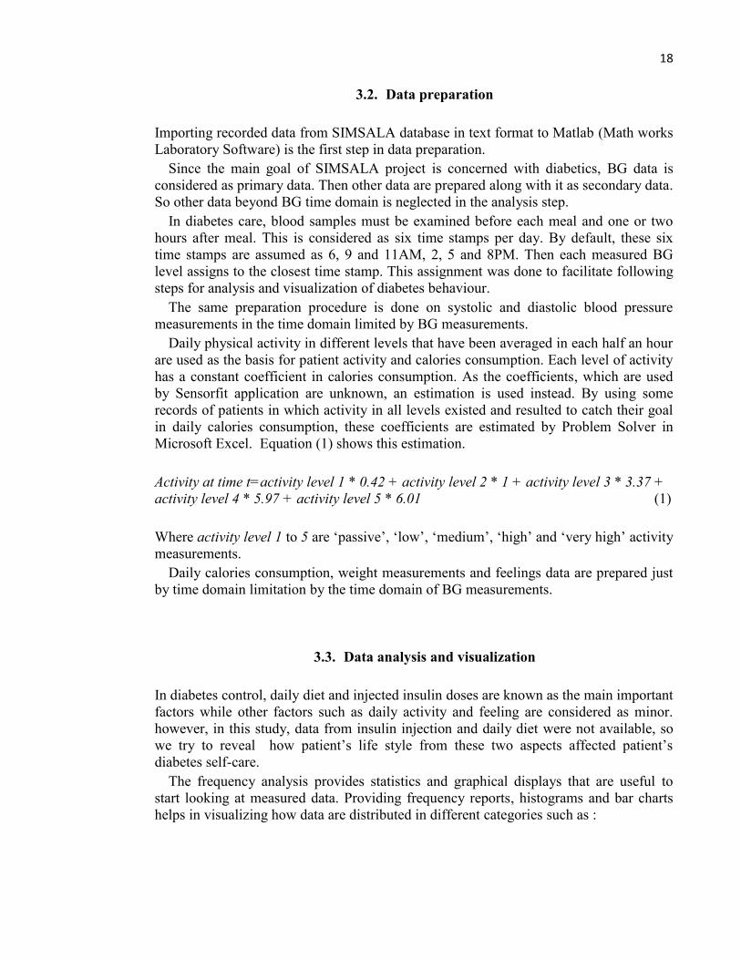
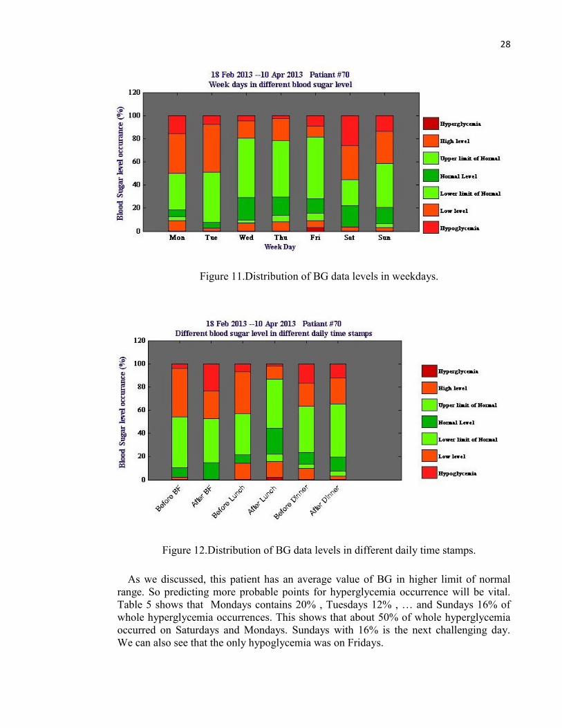
Fig. 11 and Fig. 12 are bar charts representation of these tables. Fig. 11 shows that
most hyperglycemia occurred on Saturdays then on Mondays and Sundays. Fig. 12
shows that the time after breakfast contains more percent of Hyperglycemia while the
time before and after dinner are the next.
28
Figure 11.Distribution of BG data levels in weekdays.
Figure 12.Distribution of BG data levels in different daily time stamps.
As we discussed, this patient has an average value of BG in higher limit of normal
range. So predicting more probable points for hyperglycemia occurrence will be vital.
Table 5 shows that Mondays contains 20% , Tuesdays 12% , … and Sundays 16% of
whole hyperglycemia occurrences. This shows that about 50% of whole hyperglycemia
occurred on Saturdays and Mondays. Sundays with 16% is the next challenging day.
We can also see that the only hypoglycemia was on Fridays.

29
In other hand Table 6 shows that about 32% of hyperglycemia occurred after breakfast
and 52% at dinner time mostly after it. Looking at Fig. 9 on Mondays and Saturdays, it
can be clearly seen that more challenges on Mondays are related to breakfast time and
on Saturdays are related to dinner time.
4.1.3. Secondary variables-based data analysis
Looking at patient’s daily conditions via physical activity and feeling aspects helps to
find some reasons for BG abnormality on these points. Fig. 13 shows patient’s physical
activity during study period. The vertical axes represents quantified physical activity in
0-100 range that is calculated by Equation (1).
This patient has daily physical activity in average of 40.5 (dotted line) with standard
deviation of 23. Physical activity along with body metabolism determines daily calories
consumption. Each patient has a goal for his daily calories consumption and tries to
catch this goal. As each patient’s body metabolism burns specific daily calories, more
percent of catching this goal can be considered as the result of more physical activity. So
total daily physical activity can be analyzed using the percent of this goal which is
caught. Fig.14 represents the percent of goal catch in daily calories consumption for this
patient in different days of week.
Figure 13.Average of physical activity in different time stamps of the weekdays.

30
Figure 14.Average of patient’s goal catch for daily calories consumption.
In average this patient has caught 77% of her goal for daily calories consumption.
Table 7 shows the percent of goal catch in each weekday. It is clear that this patient
burned more calories on Wednesdays, Tuesdays and Thursdays. If we look at the percent
of goal catch on Mondays and Saturdays that are previously determined as challenging
days in diabetes control, both have 66% that is less than the average value (77%). This
shows that less physical activity on Mondays and Saturdays has a role for hyperglycemia
in these days.
Table 7. Percent of patient’s goal catch for daily calories consumption in weekdays
Goal
catch (%) Monday Tuesday Wednesday Thursday Friday Saturday Sunday
Average 66 87 93 80 63 66 60
In order to analyze this patient’s activity in each daily time stamp, Table 8 and Fig. 15
are provided. If we look at time stamps 2, 5 and 6 that are previously determined as
challenging time stamps for diabetes control for this patient, time stamps 2 and 6 has
less activity among other time stamps. It can be said that less physical activity on second
and sixth time stamp (after breakfast and after dinner time) induce the BG level to
increase. As both time stamps are after meal, it is good to look at the time after lunch to
see its condition. Table 6 shows that third and fourth time stamps (time between 10:00 to
14:00) have minimum percent of hyperglycemia occurrence (4%). In other hand Table 8
shows that this patient has more activity on these time stamps (56% and 52% of goal

31
catch). This analysis confirms that more activity helps diabetics to prevent
hyperglycemia. In other hand, looking at Table 6 shows that only hypoglycemia
occurred on fourth time stamp, too. This shows the patient some points in which more
physical activity helped her preventing high BG level, but lead him to hypoglycemia. It
can be said that one challenge in diabetes control for this patient is related to regulating
amount of insulin injection or proper diet regarding to level of his physical activity to
prevent hypoglycemia.
Table 8. Distribution of physical activity in different daily time stamps
Activity TS_1 TS_2 TS_3 TS_4 TS_5 TS_6
Mean±Std 42±19 38±24 56±49 52±25 46±17 27±11
4.1.4. Data correlation
As we discussed in chapter three each exercise affects BG level within a time delay. In
order to obtain the most effective time Δt in which this patient’s BG at time t has had
significant dependency to physical activity at time t-Δt, Pearson's correlation coefficient
for each back step is calculated. As average physical activity in any half an hour has
been measured, this correlation analysis is done using step size of 30 minutes. The
procedure for maximum six hours back step is done because the first BG measurement
was assigned to 6 AM. Table 9 shows the calculated correlation coefficient for each
back step.
Table 9. Correlation between physical activity and BG level in six hours
Δt (hour) 0.5 1 1.5 2 2.5 3 3.5 4 4.5 5 5.5 6
r -0.06 -0.05 -0.06 -0.08 -0.06 -0.08 -0.09 -0.12 -0.12 -0.15 -0.17 -0.19
p 0.19 0.34 0.19 0.11 0.17 0.11 0.05 0.010 0.009 0.001 0.0002 0.0001
Based on equation (3) the significant correlation exists when correlation coefficient is
less than or equal to 0.05. Table 9 shows that BG level at each time t has significant
negative dependency on physical activity done at least 3.5 hours earlier. It is noticeable
that no diet and insulin injection parameters are considered because they were not
available. So in this calculation it is assumed that patient adhered to his diet and
prescribed insulin doses.
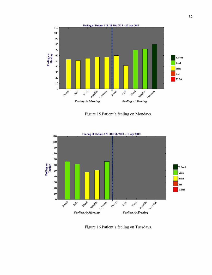
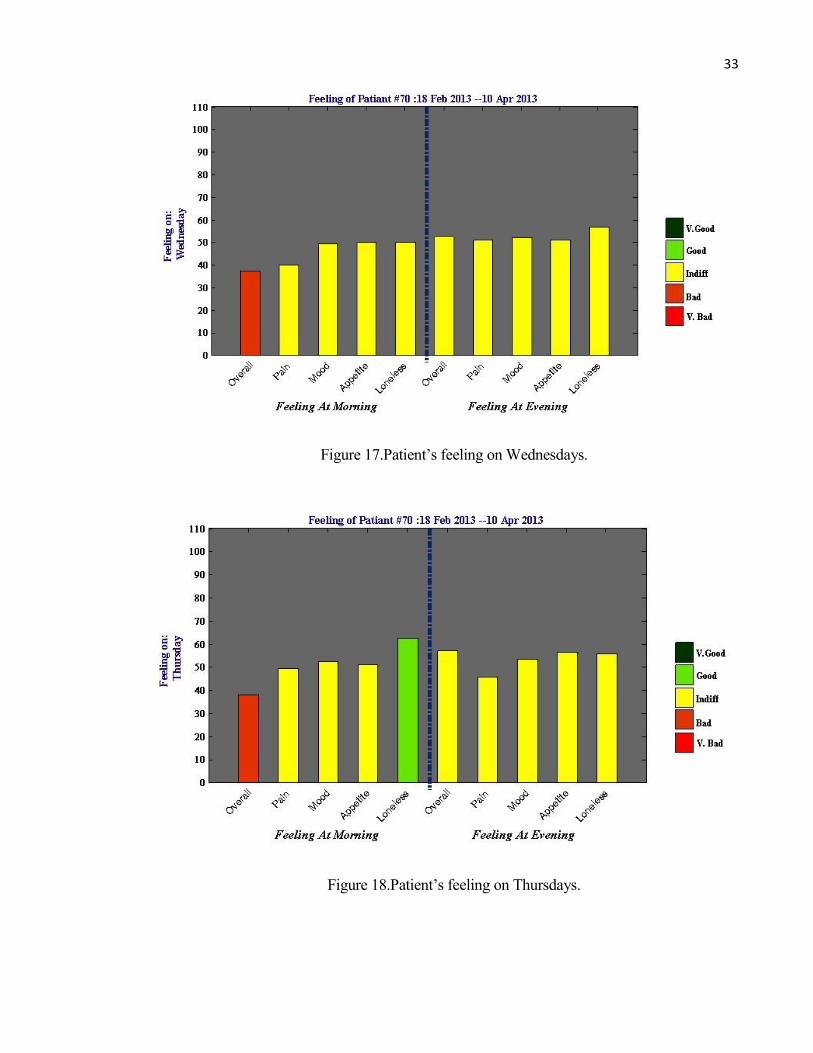
Another important parameter to analyze patient’s daily condition is his feelings which
are measured in the morning and evening via five aspects: overall, pain, mood, appetite
and loneliness. Fig. 15 to Fig. 21 shows patient’s feelings for each weekday during study
period.
32
Figure 15.Patient’s feeling on Mondays.
Figure 16.Patient’s feeling on Tuesdays.
33
Figure 17.Patient’s feeling on Wednesdays.
Figure 18.Patient’s feeling on Thursdays.

34
Figure 19.Patient’s feeling on Fridays.
Figure 20.Patient’s feeling on Saturdays.

35
Figure 21.Patient’s feeling on Sundays.
Using distinct color for each feelings level simplifies its visualization. For example in
average this patient has a good overall feeling on Sunday evenings and bad overall
feeling on Thursday mornings. Looking at Fig. 15 and Fig. 21 which represent feelings
on Mondays and Saturdays (which are previously determined as challenging days), it
can be seen that this patient had indifferent feelings on Monday’s morning and good to
very good feelings in the evening. On Saturdays, the patient had indifferent feelings in
the morning and bad overall feelings and indifferent for other feelings in the evening.
Reminding that hyperglycemia on Mondays mostly happened in the morning after
breakfast and on Saturdays in the evening before and after dinner can lead us to some
primary guess about correlation between feelings and BG level. In both cases the patient
had indifferent or bad feelings.
In order to analyze this effect more precisely, Pearson's correlation between BG data
and each feeling’s aspect is calculated and shown in Table 10. We assumed that feelings
in the morning can affect BG level until forth time stamp that is after lunch and other
time stamps are affected by feeling in the evening.
Table 10 can only reveals the significant correlation between BG level and pain
feeling in the morning. For better investigation, we can examine the correlation at each
time stamp. Table 11 to Table 16 shows correlation between BG level at each time
stamp with different feeling aspect during morning and evening.

36
Table 10. Correlation between BG data and feelings
Correlation
Feelings
Morning Evening
Overall Pain Mood Appetite Loneliness Overall Pain Mood Appetite Loneliness
p 0.20 0.02 1.00 0.75 0.76 0.17 0.56 0.15 0.46 0.45
r 0.16 0.29 0.00 -0.04 0.04 -0.21 -
0.09 -0.22 0.11 0.12
Table 11. Correlation between BG and feelings on Time stamp 1
Correlation Feelings in the morning
Overall Pain Mood Appetite Loneliness
P 0.03 0.06 0.21 0.81 0.24
r 0.50 0.43 0.29 0.06 0.28
Table 12. Correlation between BG and feelings on Time stamp 2
Correlation Feelings in the morning
Overall Pain Mood Appetite Loneliness
P 0.83 0.79 0.09 0.17 0.15
r 0.06 0.08 -0.47 -0.39 -0.41
Table 13. Correlation between BG and feelings on Time stamp 3
Correlation Feelings in the morning
Overall Pain Mood Appetite Loneliness
P 0.92 0.01 0.31 0.14 0.98
r 0.05 0.86 0.45 -0.61 0.01

37
Table 14. Correlation between BG and feelings on Time stamp 4
Correlation Feelings in the morning
Overall Pain Mood Appetite Loneliness
P 0.79 0.16 0.17 0.12 0.14
r 0.06 0.31 0.30 0.34 0.31
Table 15. Correlation between BG and feelings on Time stamp 5
Correlation
Feelings in the evening
Overall Pain Mood Appetite Loneliness
P 0.08 0.58 0.02 0.95 0.82
r -0.61 0.22 -0.75 -0.02 -0.09
Table 16. Correlation between BG and feelings on Time stamp 6
Correlation
Feelings in the morning
Overall Pain Mood Appetite Loneliness
P 0.61 0.35 0.80 0.30 0.19
r -0.09 -0.16 -0.04 0.18 0.23
Looking at these tables reveals that BG level in first half of day (morning to 3 PM)
was positively affected by overall and pain feelings in the morning and in second half of
day (after 3 PM till bed time) was negatively affected by overall and mood feelings.
In order to simplify patient’s condition in different weekdays via primary and
secondary variables points of view, a figure like Fig. 22 can be provided for each day of
week. Fig. 22 represents average of measurements on Mondays for this patient in which
BG behaviour along with blood pressure, physical activity, calories consumption goal
catch and feelings are summarized.

38
Providing such summary curves can help patient and his physician to focus on critical
days when dangerous BG levels happened. For example patient’s condition on 21 Feb. is
shown in Fig. 23. Looking at blood sugar curve shows that this patient has a deviation
from BG normal range on second time stamp. Looking at his activity and calories
consumption shows about 85% success to catch his goal. Looking at his feeling during
morning times shows a very bad overall feeling. Even though previous analysis could
approve no significant correlation between overall feeling and BG level, here, it seems
that very bad overall feelings resulted in increasing BG level in second time stamp. Such
daily summary graphs cannot prove any result but can help physician to make decision
especially by enabling him to analyzing the desired days before and after critical days.

39
Figure 22.The summary of patient’s condition on Mondays.

40
Figure 23.The summary of patient’s condition on 21 Feb.
4.2. Overall level implementation
At this level the same implementation process is done for all four patients. Then by
looking at whole data together we can obtain rate of success in their diabetes control and
reveal possible reasons leading to the rate.
4.2.1. Data distribution analysis
Table 17 reveals that BG level in patients 1 and 2 with diabetes type 2 have been
controlled in normal range or with reasonable deviation from it but in patients 3 and 4
with type 1 have been occurred in high levels. The percentage of hyperglycemia
occurrence in these patients indicates that the patients with type one dealt with more

41
challenges in their diabetes control. In other hands hypoglycemia was rarely observed in
them. In Table 18 and Table 19 distribution of secondary data in all four patients are
shown.
Table 17. BG data distribution in different levels for all patients
Patient Mean±Std
Percent of occurrence
Hypoglycemia Low
level
Lower
limit of
Normal
Normal
Higher
limit of
normal
High
level Hyperglycemia
1 5.8±0.8 0.00 1.79 1.79 56.25 40.18 0.00 0.00
2 7.6±3 0.00 5.56 1.11 30.00 52.22 10.00 1.11
3 9.5±4 0.42 5.91 2.95 13.08 42.19 24.89 10.55
4 11.9±4 0.23 1.24 1.01 4.12 37.16 33.23 23.02
Table 18. Secondary data distribution for all patients
Patient
Data Distribution
Blood Pressure Physical
activity
Calories
consumption
(%goal catch) Systolic Diastolic
1 134±8 89±8 22±12 93±6
2 163±17 85±11 21±15 81±26
3 129±7.5 83±7 41±23 77±33
4* 132.5±16 85±11 9±4.5 18.5±9
*For this patient no precise measurements for secondary variables have been done.

42
Table 19. Average feelings for all patients
Patient
Feeling in the Morning Feeling in the Evening
Overall Pain Mood Appetite Loneliness Overall Pain Mood Appetite Loneliness
1 Indifferent Indifferent Indifferent Indifferent Indifferent Good Indifferent Good Good Good
2 Bad Bad Indifferent Bad Good Bad Indifferent Bad Very bad Bad
3 Indifferent Indifferent Indifferent Indifferent Indifferent Indifferent Indifferent Indifferent Indifferent Indifferent
4 Good Good Good Indifferent Good - - - - -
4.2.2. Rate of success analysis
In Table 20 we try to clarify the rate of success for each patient to control his BG in
normal level (from lower limit to upper limit of normal range) along with the success in
meeting his goal for daily calories consumption (100%); and to have positive feeling
(indifferent, good or very good feeling) in the morning and evening.
Table 20. Rate of success for all patients
Patient
Rate of success %
BG control
(4-11 mmol/L)
Calories
consumption
goal catch
Positive feeling
in the morning
Positive feeling
in the evening
1 98 6 20 20
2 83 18 19 20
3 58 18 20 20
4 41 - - -
The rate of success in BG control in Table 20 conform to our previous discussion that
patients 1 and 2 could control their diabetes better than patients 3 and 4. But looking at
obtained rate of success in calories consumption and feeling for each patient
individually, one cannot clarify any reason leaded him to success/fail his BG control. So

43
we try to examine the whole data together for an overall analysis by categorizing BG
data in different levels, different time stamps and different weekdays.
4.2.3. Weekdays and daily time stamps analysis
The distribution of BG data in different weekdays and different daily time stamps are
shown in Table 21 and Table 22. Looking at Table 21 just highlights Fridays as most
concerning day for hypoglycemia with 50% of occurrence. Hyperglycemia occurrence
has approximately the same distribution among weekdays. Table 22 reveals the
importance of first time stamp with 40% of hyperglycemia and the time after breakfast
and after dinner with 66% of hypoglycemia.
Table 21. Distribution of BG levels in weekdays for all patients
Weekday Hypoglycemia Low
level
Lower
limit of
Normal
Normal
Higher
limit of
Normal
High
level Hyperglycemia
Monday 16.67 16.67 21.88 14.22 18.43 15.87 11.53
Tuesday 0.00 6.25 6.25 16.11 16.63 16.12 12.67
Wednesday 0.00 25.00 15.63 16.11 15.34 15.49 15.12
Thursday 16.67 18.75 21.88 18.48 12.75 15.99 17.20
Friday 50.00 12.50 9.38 15.17 12.85 12.97 13.61
Saturday 0.00 8.33 12.50 9.48 10.26 9.57 15.50
Sunday 16.67 12.50 12.50 10.43 13.75 13.98 14.37

44
Table 22. Distribution of BG levels in different daily time stamps for all patients
Time
stamp Hypoglycemia
Low
level
Lower
limit of
Normal
Normal
Higher
limit of
Normal
High
level Hyperglycemia
TS_1 16.67 14.58 9.38 36.49 20.32 31.74 40.08
TS_2 33.33 2.08 3.13 14.22 21.41 20.65 13.42
TS_3 0.00 6.25 0.00 3.32 3.78 2.77 8.13
TS_4 16.67 35.42 50.00 17.54 16.33 10.71 10.96
TS_5 0.00 22.92 21.88 12.32 18.33 12.97 9.26
TS_6 33.33 18.75 15.63 16.11 19.82 21.16 18.15
4.2.4. Primary and Secondary variables-based analysis
Another analysis is provided by Table 23 that shows BG data distribution in three
specific ranges: Normal (4-11 mmol/L), Normal to dangerous (6-11 or 3-4 mmol/L) and
Dangerous range (>=15 or <=3 mmol/L) along with the average of activity, percent of
calories consumption goal catch and feelings.
It is clear that all patients have indifferent feelings on average. So by considering it as
constant, we can see that moving from normal to dangerous range of BG level happened
simultaneously with decreasing calories consumption goal catch that is calculated from
physical activity. When percent of goal catch in daily calories consumption decreases or
in other word daily physical activity decreases, the percent of BG occurrences in
dangerous range increases, even though that the patient has proper feelings. This reveals
the importance of proper physical activity in increasing rate of success in diabetes
control.

45
Table 23. Distribution of BG data along with secondary data distribution for all patients
BG Average of Rate of success %
Range Frequency (%)
Activity Calories
consumption goal catch
Feeling in
the morning
Feeling in
the evening
Calories
consumption goal catch
Positive
feeling
in the morning
Positive
feeling
in the evening
Normal 48 26 84 Indifferent Indifferent 14 81 85
Normal to
dangerous 32 33 71 Indifferent Indifferent 17 83 81
Dangerous 20 27 67 Indifferent
to Good Indifferent 5 100 100

46
5. DISCUSSION
As a result of data analysis at customer level, the rate of success for patient #3 in his
diabetes control was determined as 58% in which he could control his BG level between
4-11 mmol/L. Regarding to his failure rate with 36% due to times when his BG level fell
in high and hyperglycemia level and 6% when in low and hypoglycemia level,
highlights that his challenges are mostly related to high level occurrences. Detailed
analysis for weekdays and different daily time stamps of this failure, specified the time
after breakfast on Saturdays and Mondays and the time before and after dinner on
Sundays as most challenging times for high level occurrences and Fridays after lunch for
low levels.
Analysis of patient’s activity on these challenging times, lead us to some primary
guess about its reasons. Regarding to the rate of success toward meeting the goal for
daily calories consumption as a parameter affected directly by daily activities, this
patient had rate of success less than average on Saturdays, Mondays and Sundays with
the rate 66%, 66% and 60% versus 77% on average. Analysis on patient’s activity in
different daily time stamps marks the time after breakfast and after dinner as less
activity. These results show the effect of less activity in increasing BG level. Inversely,
higher activities on other time stamps results in decreasing BG level. But looking at high
level of activity on time stamp four that is the time for hypoglycemia occurrence shows
that increasing activity can lead patient to hypoglycemia. This reveals another challenge
for this patient in his diabetes control which is balancing his activity with insulin doses
and proper diet to prevent hypoglycemia due to exercises. Additionally 3.5 hours has
been determined as effective time delay in which physical activity affects BG level.
Analysis of patient’s feeling on challenging times shows that he had indifferent to bad
average feelings on Monday mornings and Saturdays evenings. Calculating data
correlations between BG level and different aspect of feelings shows that patient’s BG
level on first half of days from morning till 3PM is positively affected by overall and
pain feelings measured in the morning and in second half of day is negatively affected
by overall and mood feelings measured in the evening.
Overall analysis using whole data obtained from all patients made our attention to
more challenges in diabetes control for type 1 diabetics. Looking at secondary data
leaded us to the importance of physical activity in diabetes behaviour. Considering
physical activity as basic parameter to achieve goal catch for daily calories consumption
clarifies that in spite of patient’s positive feelings in average, less success to this goal
catch results higher frequency of BG falling in dangerous range. Mathematically any
one percent failure in daily calories consumption goal catch can increase patient’s
chance to be in dangerous condition by 33%.
As shown, in this study by using data mining techniques and association rules we tried
to visualize the results in a way that creates enough motivation in patient to improve
diabetes self-care along with providing a decision support system for health providers to
improve diabetes treatment. Application of data mining in diabetes management is not a
new idea. Deepti J. [26] has provided a review on various researches concentrated on
data mining applications in diabetes management such as estimating the most important
risk factors influencing BG control, preventing diabetes incidence by analyzing its risk

47
factors, predicting diabetes dangerous complications in diabetics, developing DSCS
(Diabetes Self-care Support) service to improve diabetes self-care, estimating
effectiveness of e-health, etc. Additionally Bellazzi R. [27] has introduced similar
visualizing method by summarizing BG data in six daily time slices and weekdays as a
basis to reveal diabetes behaviour ‘at a glance’. This method has been widely used in
diabetes monitoring instruments as well as mobile applications [28]. Considering
diabetics’ life style as an important key point in diabetes treatment, this study tried to
combine this visualizing methods with some life style parameters such as activity and
emotional states. This is the point that Bellazzi R. [27] had suggested to be significantly
helpful in diabetes treatment and can improve his work. In other hands, making a variety
of daily measurements for a period as long as life time increases the complexity of
diabetes self-care especially in elderly. So we tried to minimize patient’s involvement in
daily measurements by decreasing the number of measurements to the ones that are
available through their automatically measurements such as physical activity and daily
calories consumption using mobile application. This study can be enriched by
considering more life style parameters such as daily diet and insulin doses by increasing
its accuracy to estimate the reasons for BG abnormalities.
This study can be continued by one step forward prediction in diabetes behavior which
was impossible here due to the lack of data. Monitoring diabetics for a longer time,
enables us to obtain more patterns in their diabetes behaviour which is the main
requirement of prediction. Increasing the number of life style parameters can also
improve this prediction.

48
6. SUMMARY
Diabetes mellitus, is a chronic disease that imposes unacceptably high human, social and
economic costs on all countries and needs an effective management to minimize its rate
of incidence and prevalence along with its costly and dangerous complications
worldwide. Diabetes management requires a close cooperation between the person with
diabetes and health professionals. Regarding to noticeably increasing trend in diabetes
prevalence, countries try to replace traditional face to face health care with remote
patient monitoring by taking advantages of new advances in electronics such as wireless
sensor networks and body sensors. This reduces significantly the costs and service
pressures on health centers but produce a huge amount of heterogeneous data that
confronts us with new challenges related to ‘big data’. Data mining by providing a
variety of techniques to analyze such big data and discover their hidden knowledge, has
many applications in diabetes management such as estimating the most important risk
factors influencing BG control, preventing diabetes incidence by analyzing its risk
factors, predicting diabetes dangerous complications in diabetics, developing DSCS
service to improve diabetes self-care, estimating effectiveness of e-health, etc. In this
study, another application of data mining in diabetes management which is visualizing
its behaviour using descriptive data mining and association rule in two levels including
‘customer level’ and ‘overall level’ was introduced. The goal was to visualize BG trend
along with some health and life style parameters including blood pressure, physical
activity, calories consumption, weight scale and emotional states. By clustering BG in
three different categories including daily time stamps (BFB, AFB, BFL, AFL, BFD,
AFD), weekdays and BG ranges (Hyperglycemia, High level, Higher limit of normal,
Normal level, Lower limit of normal, Low level and Hypoglycemia) and statistic
analyzing of data in each cluster stand alone or in joint with other clusters, diabetes
behaviour in each patient was visualized. This revealed critical situations that lead
patients to diabetes self-care success or failure. By calculating data correlation between
BG and physical activity or feeling, some primary reasons for this success or failure was
estimated. The accuracy of this estimation can be improved by including other life style
parameters such as daily diets and insulin doses as well as increasing the time domain of
data measurements. This also enables us to predict diabetes behaviour which plays an
important role in diabetes management.

49
7. REFERENCES
1. IDF Diabetes Atlas, 6th ed. (2013). International Diabetes Federation. URL:
http://www.idf.org/diabetesatlas. Accessed 18.2.2014.
2. Canadian Journal of Diabetes, Vol. 37 (2013). Definition, classification and
diagnosis of diabetes, Prediabetes and metabolic syndrome. Canadian Diabetes
Association. URL: www.canadianjournalofdiabetes.com. Accessed 18.2.2014.
3. Diabetes Care, vol. 35, Supplement 1 (2012). Diagnosis and classification of
diabetes mellitus. American Diabetes Association. DOI: 10.2337/dc12-s064.
4. McKinley Health Center, University of Illinois of Urbana Champaign, The
Board of Trustees of the University of Illinois (2008). Hyperglycemia. URL:
http://www.mckinley.uiuc.edu. Accessed 18.2.2014.
5. Diabetes UK (2008). Hypertension and diabetes. URL:www.diabetes.org.uk.
Accessed 18.2.2014.
6. Vermont Blueprint for Health (2007). Diabetes: lose a little weight gain a lot of
control. Vermont department of health.
7. National institute of mental health (2011). Depression and diabetes. US
department of health and human services. URL: http://www.nimh.nih.gov/health
/publications /depression-and-diabetes/index.shtml. Accessed 18.2.2014
8. Global strategy on diet, physical activity and health (2004). World health
organization. URL: http://www.who.int/dietphysicalactivity/en/. Accessed
18.2.2014.
9. Guidelines for management and care of diabetes in elderly (2003). Australian
diabetes educators association: 3.
10. World Population Ageing 2013 (2013). United Nations, Department of
Economic and Social Affairs, Population Division. DOI: ST/ESA/SER.A/348.
11. Diabetes Care. Vol. 36. Supplement 1 (2013). Standards of Medical Care in
Diabetes. American Diabetes Association. DOI: 10.2337/dc13-S011.
12. Nancy J & Bohannon, MD (1988). Diabetes in The Elderly, A unique set of
management challenges. URL: http://www.ncbi.nlm.nih.gov/pubmed/3050932.
Accessed 2.3.2014.
13. Niemi M. & Winell K. (2006). Diabetes in Finland, prevalence and variation in
quality of care. Finnish Diabetes Association.
14. Diabetes in Canada: Facts and Figures from a Public Health Perspective (2011).
Public Health Agency of Canada. URL: http://www.phac-aspc.gc.ca/cd-mc/
diabetes-diabete /index-eng.php . Accessed 22.2.2014.
15. Diwani S, Mishol S, Kayang D, Machov D & Sam A (2013). Overview
applications of data mining in health care: The case study of Arusha region.
International journal of computational engineering research. Vol. 3 . Issue 8.
16. Muhamad HMA, Wahidah H & Nuraini AR (2012). Data mining for medical
systems: A review. Proc. International conference on advances in computer and
information technology. ACIT 2012.
17. Berson A, Smith S & Thearling K (2005). An overview of data mining
techniques. URL: http://www.thearling.com/text/dmtechniques/dmtechniques.
htm. Accessed 24.2.2014.

50
18. Che D, Safran M & Peng ZH (2013). From big data to big data mining:
challenges, issues and opportunities. B. Hong et al. (Eds.): DASFAA Workshops
2013, LNCS 7827: 1–15.
19. Edjlali R (2011). Information 20/20: Focus, connect and lead with information.
Gartner Inc.
20. Davenport H (2013). Big data executive survey 2013: The state of big data in the
large cooperate world. New Vantage Partner LLC.
21. Aljumah A, Ahmad MG & Siddiqui MK (2013). Application of data mining:
Diabetes health care in young and old patients. Journal of King Saud University
Computer and Information Sciences:127-136.
22. Rajesh K & Sangeetha V (2012). Application of data mining methods and
techniques for diabetes diagnosis. International journal of engineering and
innovative technology. Vol. 2. Issue 3.
23. Kaur H & Wasan SK (2006). Emperical study on applications of data mining
techniques in healthcare. Journal of computer science 2(2). S194-S200
24. Marinov M, Mohammad Mosa AS, Yoo I & Boren S (2011). Data mining
technologies for diabetes : A systematic review. Journal of diabetes science and
technology, Vol. 5, Issue 6.
25. Sa-ngasoongsong A & Chongwatpol J(2012). An analysis of diabetes risk factors
using data mining approach. Oklahoma state university, USA.
26. Deepti J & Divakar S (2013). A Review on associative classification for Diabetic
datasets, A Simulation Approach. International journal of computers and
technology, Vol. 7, No. 1.
27. Bellazzi R & Abu-Hanna A (2009). Data Mining Technologies for Blood
Glucose and Diabetes Management. Journal of diabetes science and technology,
Vol. 3, Issue 3.
28. Bin-Sabbar MS & Al-Rodhaan MA (2013). Diabetes Monitoring System Using
Mobile Computing Technologies. International journal of advanced computer
science and applications, Vol. 4, No. 2.
29. Lindholm M.(2012). Distributed system for wireless monitoring of the wellbeing
of the seniors. Master’s Thesis. University of Oulu, Department of Computer
Science and Engineering.
30. Sorvala A (2012). Kaatumisen ilmaisu ja aktiivisuuden luokittelu seniori-ikäisten
kotona asumisen tukena. Diplomityö. Oulun yliopisto, sähkötekniikan osasto.