Embed Size (px)
Citation preview

SGP-TR- 152
Description of Heterogeneous Reservoirs Using Pressure
and Tracer Data
Xianfa Deng
March 1996
Financial support was provided through the Stanford Geothermal Program under
Department of Energy Grant No. DE-FG07-90IDI2934, and by the Department of Petroleum Engineering,
Stanford University
Stanford Geothermal Program Interdisciplinary Research in Engineering and Earth Sciences STANFORD UNIVERSITY Stanford, California

@ Copyright 1996 by Xianfa Deng
All Rights Reserved
.. 11

Abstract
This study investigated met hods of characterizing areally heterogeneous reservoirs
through the interpretation of pressure data and tracer data. The analysis of pressure
data and the analysis of tracer data were studied both individually and simultane-
ously.
A nonlinear least square method was applied to interpret multiwell transient pres-
sure data from interference tests. Several models, including anisotropic reservoir,
circular discontinuity, no-flow linear boundary and interaction among multiple wells
were investigated. Their solutions were reformulated to fit into the nonlinear regres-
sion algorithm. Results showed that using multiwell data avoids inconsistent results
for the selected reservoir model, increases the tolerance to noise in the data, increases
the confidence of the interpretation and improves the convergence of the regression
search.
Analytical solutions to tracer flow were obtained for three cases: radial flow,
linearly varying dispersivity and linear flow in composite reservoir. Another semi-
analytical solution to tracer flow in two dimensional reservoirs based on the charac-
teristic method is presented.
The method of Green’s functions has been a powerful tool to solve unsteady flow
problems in homogeneous reservoirs. The application of the Green’s function method
was extended to diffusivity problems in heterogeneous reservoirs. A fundamental
formula was obtained to express the general pressure solution to the diffusivity equa-
tion with nonhomogeneous initial and boundary conditions in terms of Green’s func-
tions. Through practical examples, appropriate methods were suggested for obtaining
Green’s functions that are more difficult to find in heterogeneous problems than in
iv

homogeneous ones. Reciprocity is a basic and useful property which facilitates the
understanding to porous media flow problems. With the Green’s function method
developed, the conditions under which the Principle of Reciprocity holds in hetero-
geneous formation were studied. The application of the Green’s function method to
convection-dispersion equation and its limitations are also discussed.
After the analysis of pressure data and tracer data are described individually, di-
rect method is presented to simultaneously interpret pressure data and tracer data
from multiple wells to characterize the areal permeability distribution in heteroge-
neous reservoirs. Since tracer data are more sensitive to heterogeneity than pressure
data, integration of the two kinds of data should give a better description of the
reservoir. A correlation between permeability and dispersivity was investigated, and
used to reformulate the convection-dispersion equation and diffusion equation to a
system of first-order equations in permeability. The system of equations can then
be solved to yield the permeability distribution for appropriate boundary conditions.
Advantages and disadvantages of this new scheme are discussed. As an example, the
time function method was applied to the interpretation of pressure and tracer data
of a multiwell reservoir with a circular discontinuity.
V

Contents
Abstract iv
Acknowledgements vi
1 Introduction 1
2 Use of Pressure Data from Multiple Wells 7
2.1 Multiwell Data of Anisotropic Reservoir . . . . . . . . . . . . . . . . 7 2.1.1 Mathematical Considerations . . . . . . . . . . . . . . . . . . 8 2.1.2 Field Example . . . . . . . . . . . . . . . . . . . . . . . . . . . 9
2.2 Heterogeneity of the Circular Discontinuity Type . . . . . . . . . . . 16
2.2.1 Discontinuity Without Wellbore Storage . . . . . . . . . . . . 17 2.2.2 Discontinuity with Wellbore Storage . . . . . . . . . . . . . . 24
2.2.3 Transformation of Coordinate System . . . . . . . . . . . . . . 26 2.2.4 Objective Function . . . . . . . . . . . . . . . . . . . . . . . . 28
2.2.5 Examples . . . . . . . . . . . . . . . . . . . . . . . . . . . . . 35
2.2.6 A Special Case - Concentric Active Well . . . . . . . . . . . . 38
2.4 No-Flow Linear Boundary . . . . . . . . . . . . . . . . . . . . . . . . 59 2.3 Analysis of Drawdown-Buildup Pressure Data in Multiwell Systems . 47
2.5 Interpreting Multiwell Pressure Data of Ohaaki Geothermal Field . . 63
3 Green’s Functions and the Reciprocity Principle in Heterogeneous Media 72
3.1 Definition of Green’s Functions . . . . . . . . . . . . . . . . . . . . . 72
.. v11

3.2 Properties of Green’s Functions . . . . . . . . . . . . . . . . . . . . . 75
3.3 Pressure in Terms of Green’s Functions . . . . . . . . . . . . . . . . . 76
3.4 Examples of Green’s Functions . . . . . . . . . . . . . . . . . . . . . 76
3.4.1 Case 1: Separation of Variables . . . . . . . . . . . . . . . . . 76
3.4.2 Case 2: Fourier Transformation . . . . . . . . . . . . . . . . . 78
3.4.3 Case 3: Working in Laplace Space . . . . . . . . . . . . . . . . 80
3.4.4 Case 4: Decomposition . . . . . . . . . . . . . . . . . . . . . . 82 3.5 Anisotropic and Heterogeneous Reservoirs . . . . . . . . . . . . . . . 84
3.6 Principle of Reciprocity . . . . . . . . . . . . . . . . . . . . . . . . . . 85
3.7 Effects of Wellbore Storage and Skin . . . . . . . . . . . . . . . . . . 86
3.8 Green’s Functions for Tracer Flow Problems . . . . . . . . . . . . . . 88
4 Analytical Solutions to Tracer Flow 90
4.2 Linear Tracer Flow in a Composite Reservoir . . . . . . . . . . . . . . 95 4.1 Convection-Dispersion Equation with Linearly Changing Dispersivity 92
4.3 Radial Convection-Dispersion Tracer Flow in Homogeneous Reservoir 103
4.4 Streamlines in an Infinite Reservoir with a Circular Discontinuity . . 104
5 Using Tracer and Pressure Data Simultaneously 113
5.1 Dispersivity and Permeability Correlation . . . . . . . . . . . . . . . 113
5.3 Ill-posedness . . . . . . . . . . . . . . . . . . . . . . . . . . . . . . . . 116
5.4 Permeability Constraints . . . . . . . . . . . . . . . . . . . . . . . . . 118
5.5 Direct Method for Tracer Data . . . . . . . . . . . . . . . . . . . . . 121 5.6 Example . . . . . . . . . . . . . . . . . . . . . . . . . . . . . . . . . . 125
5.2 Integrating Tracer and Pressure Data in Heterogeneous Reservoirs . . 115
6 Conclusions 136
A Equivalence of two Anisotropic Solutions 142
B Pressure Expression in Green’s Function 146
C Reciprocity of Green’s Function 150
... V l l l

D Two-Dimensional Green’s Functions in Problems with Variable Per- meability 154
E Pressure and Tracer Solutions for a Multiwell Heterogeneous Sys- t em 158
Nomenclature 164
Bibliography 168
ix

List of Tables
2.1 Water-injection interference pressure rise above the initial pressure . . 11
2.2 Configuration of the formation . . . . . . . . . . . . . . . . . . . . . . 28
2.3 Generated pressure data for the reservoir of Example 1 . . . . . . . . 36
2.4 Properties of the reservoir in Example 1 . . . . . . . . . . . . . . . . 37
2.5 Initial guess, matching result and true value . . . . . . . . . . . . . . 38
2.6 Generated pressure data of Example 2 . . . . . . . . . . . . . . . . . 39
2.7 Properties of the reservoir for Example 2 . . . . . . . . . . . . . . . . 40
2.8 Initial guess, matching result and true value . . . . . . . . . . . . . . 40

List of Figures
2.1
2.2
2.3
2.4
Field well pattern in an anisotropic reservoir . . . . . . . . . . . . . . Using three sets of pressure data in an anisotropic reservoir example . TJsing nine sets of pressure data in an anisotropic reservoir example .
Using another three sets of pressure data in an anisotropic reservoir
example . . . . . . . . . . . . . . . . . . . . . . . . . . . . . . . . . .
Pressure response versus compressibility of first region . . . . . . . . . 2.5 Infinite reservoir with a circular discontinuity . . . . . . . . . . . . . 2.6
2.7 Pressure response versus permeability of first region . . . . . . . . . . 2.8 Pressure response versus compressibility of second region . . . . . . . 2.9 Pressure response versus permeability of second region . . . . . . . . 2.10 Pressure response versus position of active well (distance) . . . . . . . 2.11 Pressure response versus position of active well (angle) . . . . . . . . 2.12 Pressure response versus radius of discontinuity . . . . . . . . . . . . 2.13 Comparison of pressure response in active well with or without wellbore
storage . . . . . . . . . . . . . . . . . . . . . . . . . . . . . . . . . . . 2.14 Comparison of pressure response in observation well with or without
wellbore storage . . . . . . . . . . . . . . . . . . . . . . . . . . . . . . 2.15 Transformation of two coordinate systems . . . . . . . . . . . . . . . 2.16 Well pattern for an infinite reservoir with a circular discontinuity . .
2.17 Objective function versus various position of active well . . . . . . . . 2.18 Objective function versus various position of active well . . . . . . . . 2.19 Objective function versus various position of active well . . . . . . . . 2.20 Objective function versus various position of active well . . . . . . . .
10
12
14
15
18
20
20
21
21
22
22
23
25
25
27
29
30
31 32
33
xi

2.21 Comparison of pressure responses between skin factor approach and
discontinuity approach . . . . . . . . . . . . . . . . . . . . . . . . . . 2.22 Comparison of pressure responses between skin factor approch and
discontinuity model approach . . . . . . . . . . . . . . . . . . . . . . 2.23 Matching result for concentric model
2.24 Matching result for concentric model
2.25 Interference pressure response versus production time . . . . . . . . .
. . . . . . . . . . . . . . . . . .
. . . . . . . . . . . . . . . . . .
2.26 Pressure response versus production time and wellbore storage effect . 2.27 Pressure response versus production time and wellbore storage effect . 2.28 Pressure response versus production time and wellbore storage effect .
2.29 Pressure response versus production time . . . . . . . . . . . . . . . . 2.30 Pressure response versus production time and wellbore storage effect . 2.31 Pressure buildup response versus time after shut-in . . . . . . . . . . 2.32 Pressure buildup versus time after shut-in and wellbore storage effect
2.33 Configuration of six-well and infinite-well systems . . . . . . . . . . . 2.34 Pressure response versus production time . . . . . . . . . . . . . . . . 2.35 Pressure response versus production time and wellbore storage effect . 2.36 Pressure buildup response versus time after shut-in
2.38 Drawdown pressure response versus production time . . . . . . . . . .
. . . . . . . . . . 2.37 Pressure buildup versus time after shut-in and wellbore storage effect
2.39 Drawdown pressure response versus production time . . . . . . . . . 2.40 Well pattern for an infinite reservoir with a linear no-flow boundary .
2.41 Contour of objective function using two sets of pressure data . . . . . 2.42 Contour of objective function using three sets of pressure data . . . . 2.43 Approximate matching results from Leawer e t al (1988) . . . . . . . . 2.44 Matching results without weights and initial pressures as parameters . 2.45 Matching results with initial pressures as parameters . . . . . . . . . 2.46 Matching results with weights emphasizing early data . . . . . . . . . 2.47 Matching results with initial pressures as parameters . . . . . . . . . 2.48 Matching results with weights and initial pressures as parameters . .
42
43
44
45
48
48
49
49
51
51 52
52 53 55
55
56
56
58
58
60 61
62
66 67
68 69 70
71
.. xii

3.1
4.1
4.2
4.3
4.4 4.5
4.6
4.7
4.8
4.9
4.10
4.11
4.12
4.13
4.14
5.1
5.2
5.3
5.4
5.5
5.6
5.7
5.8
5.9
Distribution of mobility and storativity . . . . . . . . . . . . . . . . . 82
Tracer responses(inc0rrect) calculated by Stehfest algorithm . . . . . 93
Tracer response(correct) calculated by Crump algorithm . . . . . . . 93
Linear tracer flow in composite region . . . . . . . . . . . . . . . . . . Tracer profile in one dimensional uniform region . . . . . . . . . . . . Tracer profile in one dimension with two different dispersivities . . . . Tracer profile in one dimension with two different dispersivities . . . . Tracer profile in one dimension with two different porosities
Streamlines of two wells in a homogeneous reservoir . . . . . . . . . .
Comparison of constant dispersivity and linearly changing dispersivity 94
96
98
98
99
99
106
107
108
109
111
111
. . . . . Pressure distribution of two wells in discontinuous reservoir . . . . . .
Streamlines of two wells with a discontinuity of lower permeability . . Streamlines of two wells with a discontinuity of higher permeability .
Tracer profile in a doublet system of infinite reservoir
Tracer profile in a doublet system of infinite reservoir
. . . . . . . . .
. . . . . . . . .
Propagation of concentration of discontinuity at x = 0 . . . . . . . . 124
x-y-t diagram showing characteristic surface for the concentration of
radialflow . . . . . . . . . . . . . . . . . . . . . . . . . . . . . . . . . 124
Pressure distribution of multiwell system with a circular discontinuity 126 Pressure contour of multiwell system with a circular discontinuity . . 126
128
Streamline of multiwell system but without the circular discontinuity 128
Concentration front in the multiwell system with a circular discontinuity129
Concentration front in the multiwell system without the circular dis-
continuity . . . . . . . . . . . . . . . . . . . . . . . . . . . . . . . . . 130
x-y-t diagram showing the time at which the concentration front arrives
as a function of (x, y) . . . . . . . . . . . . . . . . . . . . . . . . . . .
Streamline of multiwell system with a circular discontinuity . . . . . .
131
5.10 The time at which the concentration front arrives as a function of (x. y)131
5.1 1 Permeability distribution calculated using pressure and tracer data
from 300 by 300 observation points . . . . . . . . . . . . . . . . . . . 133
... Xll l

5.12 Permeability distribution calculated using pressure and tracer data
from 100 by 100 observation points . . . . . . . . . . . . . . . . . . . 134 5.13 Permeability distribution calculated using pressure and tracer data
from 30 by 30 observation points . . . . . . . . . . . . . . . . . . . . 135
xiv

Chapter 1
Introduction
Pressure tests and tracer tests are used frequently to estimate parameters and identify
flow paths in geothermal reservoirs that are often controlled by the large heterogeneity
in permeability due to fractures.
The use of tracer tests to determine the nature of the flow paths in geothermal and
groundwater reservoirs was studied broadly in the 1980s. Jensen and H o m e (1983) developed a matrix model to obtain the tracer returns from fractured reservoirs. A similar model was used to forecast the thermal breakthrough from tracer test data by
Walkup and H o m e (1982). A single well tracer test in fractured geothermal reservoirs
was studied by Kocabas and H o m e (1987). Due to the geometric complexity in
representing the fractures, all these models were applied only to systems with one or
two fractures. There has been little work done in solving the tracer problem for a
multiply fractured reservoir that also includes the geometric effects of the fractures.
Tracer tests are believed to be more sensitive to heterogeneity than pressure tests.
Pressure interference tests are good for determining directional permeability trends
and the average properties between two wells, while well-to-well tracer tests indi-
cate the extent of heterogeneity that is merely averaged in the pressure interference
tests. These two types of tests describe different characteristics of the reservoir.
Thus, running both tests may be helpful. In addition, obtaining both pressure and
tracer data should help in reducing the uncertainty or nonuniqueness in the solutions.
Nonuniqueness always arises with either tracer test analysis or pressure test analysis
I

CHAPTER 1. INTRODUCTION 2
alone because the property identification problem is under-determined when the het-
erogeneity is represented as a spatial function. It is important to coordinate different
studies, such as geology, geophysics, coring, well logging, pressure testing and tracer
testing etc. so that the interpreted properties of the reservoir are compatible with
all the sources of information. The central emphasis of this work is on combining
pressure data and tracer data from multiple wells.
Among the efforts to integrate tracer data with other type of data, Hyndrnan (1993) presented the Split Inversion Method to combine crosswell seismic and natural gra-
dient tracer tests data in a process-oriented parameter estimation algorithm. This iterative method can estimate the location and shape of large-scale lithologic zones,
and the mean seismic velocity, hydraulic conductivity, and dispersivity within each
zone. Peters and AfzaZ (1992) made effort in other direction by using CT imaging
data of the media to estimate permeability and porosity distributions. The model
developed was for one-dimensional linear incompressible flow of stable displacement
in laboratory-scale porous media.
The convection-dispersion equation has been the model used most commonly to
describe transport phenomena in porous media. Bear (1961) considered the concen-
tration distribution, in two dimensions, resulting from a point tracer injection into a
uniform macro-flow and showed that an approximated variance of this concentration
distribution yields a tensorial coefficient of dispersions DiJ, and that this tensor could
be related to a fourth rank dispersivity tensor q + l , the components of which were de-
termined by geometrical characteristics of the porous medium only. De Jossenlin de
Jong and Bossen (1961) subsequently established a dispersion equation on this basis,
valid for three-dimensional convective tracer transport through an isotropic porous
medium. De Jossenlin de Jon9 and Bossen (1961) showed that the dispersion tensor
resulting from Bear’s analysis could be written
Abbaszadeh-Dehghani (1982) developed the analytical solutions to immiscible dis-
placements for a variety of repeated flooding pattern. The dispersion effects were

CHAPTER 1. INTRODUCTION 3
considered by computing the concentration of the displacing fluid along the stream-
lines. For heterogeneity, Abbaszadeh-Dehghani (1982) studied a stratified model with-
out layer communication. These noncommunicating layered systems were further
investigated by Mzshra (1987) together with both pressure and tracer data. The
result Mishru (1987) reached indicated that tracer data convey more information
than pressure data for describing layered systems. Mishra (1987) also introduced the
heterogeneity index &(,,)AD defined as the product of permeability variance and a
dimensionless correlation length scale to describe the permeability difference. The
effects of large or small heterogeneity index on tracer flow were compared.
Yu (1984) studied a one-dimensional, uniform, vertical flow of radioactive nuclide
in a homogeneous, saturated porous medium with instantaneous adsorption and the
linear Freundlich isotherm. Linear and nonlinear least square methods were used to
estimate the parameters iteratively.
Compared to the tracer problem, pressure problems are usually easier to solve
analytically. There are a wide variety of analytical well test analysis models in the
literature. In particular, the Green’s function method has been found to be an effec-
tive analytical tool to construct pressure responses in homogeneous reservoirs.
Using the Green’s function method to solve linear ordinary and partial differen-
tial equations is not a new idea. However, many of the textbooks of mathematics
only cover the application of this method to simple equations. Starkgold (1979) and
Roach (1982) showed some examples how to use this method for equations of parabolic
and hyperbolic equations with constant coefficients. The method of Green’s func-
tions has been a powerful tool to solve unsteady flow problems for homogeneous
reservoirs in petroleum engineering. De Wiest (1969) used this method in a prob-
lem of water flowing through porous media. Gringarten and Ramey (1973) made
this approach practically useful in petroleum engineering by giving tables of Green’s
functions for pressure diffusion in homogeneous or anisotropic reservoirs. Ozkan and
Raghavan (1991) extended these tables and provided solutions in Laplace space, as
well as for naturally fractured reservoirs. Carslaw and Jaeger (1959) discussed the
Green’s function approach for problems of heat conduction; however, their definition
of Green’s function is less useful if applied to composite or heterogeneous regions.

CHAPTER 1. INTRODUCTION 4
A subtle, yet important aspect of using Green’s functions in heterogeneous prob-
lems is their dependence on the Principle of Reciprocity. By investigating the condi-
tions under which reciprocity holds, we were able to illustrate those problems whose
solutions are accessible by use of Green’s functions.
The principle of reciprocity is also useful in understanding reservoir physics.
Mcl<inley e t al. (1968) investigated the effect of this property in the analysis of in-
terference well testing. Ogbe (1984) studied this principle in the presence of wellbore
storage and skin effect for infinite reservoirs. McKinley et al. (1968) proved that
this principle holds if the mobility and storativity are continuously distributed. We
were able to show that the principle can also be extended to discontinuous distribu-
tions of reservoir properties, and also investigated the influence of wellbore storage
on reciprocity.
Most studies of well test analysis start by solving the diffusivity equation in which
permeability or dispersivity and porosity are treated as coefficients. For instance, the
pressure equation is solved to yield pressure for specific boundary conditions. Once
this mathematical model is formed, the pressure response can be calculated for any
given permeability and porosity. The remaining work in the analysis is to compute
the correct pressure curve to match the real data and infer the needed permeability.
In computer-aided interpretation, an initial permeability value is estimated, then
the pressure response is obtained and compared with the observed pressure data.
Based on the difference, the estimate is adjusted iteratively. This iterative process is
referred to as the Output Error Criterion by Yeh (1986). When a large set of data
is involved, this approach will require a large amount of calculation and sometimes
becomes inefficient and impractical. One of the solutions to this problem is to put a
filter in front of the interpreter. The filter serves to choose a subset from the whole
set of data. The question then becomes which subset is a good representation and
how to avoid inconsistent results interpreted from different subsets. This problem
is not easy to solve either. Moreover, the minimization of an error criterion defined
on the difference between the computed and observed data may be associated with multiple local convergences.
There also exist cases that defeat the output error procedure as shown by Fulk (1983).

C H A P T E R 1. INTRODUCTION 5
Even though conditions can be specified to guarantee the unique determination of the
permeability k ( z , y) , the optimization approximations k;j do not necessarily converge
to the unique function k ( z , y ) as the grid spacing decreases. Nonetheless, for the
output error procedure, the possibility of using regularization method or constrained
optimization can make the methods attractive in some cases.
Besides this conventional approach, there have been some attempts to identify
the parameters by solving the diffusivity equation from the opposite direction. One
type of the parameter identification approach was called the Direct Method in aquifer
studies, e.g. Sugar et al. (1975)) also referred to as the Equation Error Criterion by
Yeh (1986). In this approach, taking the equation
8 a P 823 (3 8 P 8 P qP -(k- + IC- ) + - ( I C - + k-) = - ax ax ay ay ax ay h
as an example, the permeability values are considered as dependent variables of pres-
sure in the form of a formal boundary value problem. If the pressure p is known
everywhere, then 2, f$ 3 and 3 are also known, and the equation becomes a
linear first-order hyperbolic equation in terms of permeabilities. Yeh e t al. (1983)
applied this method to an unsteady flow in a heterogeneous, isotropic, and confined
aquifer. There, kriging was used as a presampling filter for reconstruction and the
parameter was estimated by using a multiobjective optimization criterion to find the
optimum dimension.
Nelson (1968) presented a direct method for a steady flow system called the en- ergy dissipation method which was based on the characteristic equation. This method
requires a boundary condition on permeability since the equation was reduced to a
first-order partial differential equation in the unknown permeability. For pressure
interpretation, the finite element method has also been employed in approximating
pressure and permeability, e.g. Frind e t al. (1973) and Yeh e t al. (1983). An alge-
braic method was developed by Sugar (1975) and its error bound was obtained by
Yakowitz (1976). This technique utilized the idea that the effect of the permeability
value at a location is uniquely determined by values of pressure in a neighborhood of
the location.
The direct approach has not yet been widely applied to the tracer equation. With

CHAPTER 1. INTRODUCTION 6
the assumption that there is a correlation between dispersivity coefficients and perme-
abilities, both the tracer equation and the pressure equation will have permeabilities
as parameters, then permeabilities could be solved directly as unknowns in both the
pressure and tracer equations. The interpretation of pressure data and tracer data
together should provide a better estimation of the permeability distribution in het-
erogeneous reservoirs.
The goal of this study was the interpretation of pressure data and tracer data for
multiwell systems. First, the multiwell pressure data were investigated for several
heterogeneous models with analytical pressure solutions. The methods for finding
solutions to tracer problems were studied with an emphasis on analytical methods.
Then, the Green’s function method was established for both diffusivity equation and
convection-dispersion equation with an investigation of the principle of reciprocity.
Finally, an approach to integrate pressure and tracer data to estimate areal perme-
ability distribution was investigated.

Chapter 2
Use of Pressure Data from
Multiple Wells
Considering the amount of data collected in well test analysis, there are two oppo-
site scenarios that require special attention: more data than necessary and insuffi-
cient data. In the first case, interpretation results by conventional methods may be
nonunique depending on the sufficient subset of data chosen and usually, it is difficult
to tell which answer is correct or better. One way to avoid the nonuniqueness in this
approach is to interpret all the applicable data sets simultaneously.
In t,his chapter, a nonlinear least square method is presented to analyze multiwell
transient pressure data for various reservoir models that have simple heterogeneities
such as anisotropy, circular discontinuity or no-flow boundary. In a multiwell system,
neighbor wells in production have influence on the buildup pressure data from ob-
servation wells. The interaction among multiple active and testing wells is discussed
in Section 2.3. Section 2.5 applies the nonlinear least square method to interpret
multiwell data from the Ohaaki geothermal field.
2.1 Multiwell Data of Anisotropic Reservoir
For an anisotropic formation, the directional permeabilities are the parameters of
interest as they play an important role on planning reservoir development such as fluid
7

C H A P T E R 2. USE OF PRESSURE DATA FROM MULTIPLE W E L L S 8
injection. In the 1960s, there appeared a series of papers on the well test analysis for
anisotropic aquifers in groundwater hydrology. The type-curve matching method for
multiple observation wells recommended by Papadopulos (1965) and Wnlton (1970)
averages the pressure-scale match points to avoid different pressure-scale matches
that may be found for various observation wells. Based on the observation that the
pressure scale in pounds per square inch is the same for all the sets of field data,
as indicated in the solution of anisotropic formation, Barney (1975) outlined another
approach to simply align the pressure scale and adjust the time scale until all sets
of field data match. However, due to noise in real data, the pressure scale matched
from the pressure data of one well may not be the same as that matched from other
wells. Nonunique results may arise when the matching starts with the pressure data
of a different well. Furthermore, the method can only make use of pressure data from
three wells. Choosing a typical set of three wells from multiple wells is not easy.
2.1.1 Mat hemat ical Considerat ions
The theory of fluid flow through an anisotropic medium has been well established.
Consider a, well producing at a constant rate in an infinite anisotropic medium with
three permeability components as IC,,, ICxy, kyy. The thickness h and porosity 4 of
the medium are constant.
Collins (1961) chose the permeability axes as the coordinates system axes. A
solution to the governing equation
d2P a 2 P 8P k x x - + b Y Y 7 = $pet-- 3x2 dY dt
for infinite-acting radial flow was obtained as
where kxx and k y y are principal permeabilities. From the general governing equation
Papadopulos (1965) derived another solution using Fourier transformation and Laplace
transformation

C H A P T E R 2. USE OF PRESSURE DATA FROM MULTIPLE WELLS 9
kxx - kxx 6 = arctan ( k,y ) (2.7)
Though these two solutions are mathematically equivalent as shown in Appendix A, the solution presented by Papadopulos (1965) is more convenient for the analysis of
observed pressure data since the permeabilities or permeability axes are unknowns in
well test analysis.
When more pressure data than needed are present, using all the sets of data
Estimating the directional can be achieved by nonlinear least square regression.
permeabilities is transformed as to minimize the following objective function
where Q = d-, fl = kxx , y = IC,, and Ap;,At; are the measured pressure
and time; x;,y; are the positions of wells from which Ap;,At; are measured. There
exist many methods to solve nonlinear least square problems. Among them, the
Marquardt (1963) method works well for anisotropic formations if a restriction is
posed that /?-y - a = 0.001 when & - a < 0.
2.1.2 Field Example
The field example presented by Ramey (1975) was interpreted in this section using
the nonlinear square a,pproach.
In order to determine whether directional permeability would influence the pro-
duction in a watered out formation, an injection well test was run. Fig. 2.1 represents

C H A P T E R 2. USE OF PRESSURE DATA FROM MULTIPLE WELLS
1 -C(-470,430) e
Y L
b 1 -D(0,475)
1 -E(475,514) e
5-C(-455,0) ) X
5-E(475,0)
Figure 2.1: Field well pattern in an anisotropic reservoir
9-C( -470, -460)
0 0
9-E(470,-415)
10

C H A P T E R 2. USE OF PRESSURE DATA FROM MULTIPLE WELLS 11
Table 2.1: Water-injection interference pressure rise above the initial pressure
Well 1-D
25
Well 1-E 1 Well 5-C 1 Well 5-E
47 5 71 17.2 47 72 11 94 24 72 95 13 113 25.1 94 115 16 124 26 115 125 16 122
AP 4 11 16.3 21.2 22 25
Well 9-D 1 Well 9-E I At 23.5 28.5 51 75 95 120
23.2 94 10 27.2 115 12.5 27 125 13
the well pattern where well 5-D served as a single injection well and the surrounding
wells (5-E, 1-E, 1-D, LC, 5-C, 9-C, 9-D and 9-E) were observation wells. The ris-
ing parts of the pressure(psi) and time(hours) are presented in Table 2.1. Table 2.1
represents a set of interference data from seven wells, which is more than required to
obtain a unique result since only three sets of the data are needed to determine IC,,, IC,,, k,, and $c. Using Wells 5-E,l-E and 1-D, Barney (1975) obtained by manual
type curve matching:
= 15.2 md
k,, = 19.4 md
IC,, = 3.12 md,
while for the same set of data, a nonlinear least square method gives the solution
k,,z = 15.59 md
k,, = 19.59 md
IC,, = 2.07 md
as shown in Fig. 2.2. The noticeable difference is the IC,, value. The initial guesses
used in the nonlinear least square algorithm are:

C H A P T E R 2. USE OF PRESSURE DATA FROM MULTIPLE WELLS 12
ool LLJ 10 1W 1000 loo00 0 1
dehal
I I 10 well 5-c
P B l;
O 1 f 001 I , , # , I , 1 , , , , I , , , , , , , , I , , , , , , , 1 , , /,,j
IO 100 lo00 loo00 0 1 dehal
Well9-E
lo €-- I " '" I ' " I
10 100 loo0 loo00 0 1 delal
0 0 1 1 , 1 1 , , , , I , , , , , , , , I , , , , , , , 1 , , , , , , , , 1 , , , , , 0 1 1 10 100 1OW 1 woo
denat
10 Well 9-c I ' ' " " " I ' 3 " " ' I ' ' " " " I ' ' ' 1 '
-
0 1 1 0 0 1 t 1 1 8 8 8 , , , , , , , , 1 , , , , , , / I , , , , 1 , , , , , , ,
0 1 1 10 100 1000 loo00 dehat
1 0 . Well9.D I ' ' " " ' I ' ' " " ' 1 ' ' ' ' ' ' ' I ' ' ' ' "
,
0 01 0 1 0 1 4 10 100 1Mx) 1WM) deiiat
Match Data Sets of
Well l -E Well 5-E Well l -D
Kxx Kyy Kxy 15.59 19.59 2.07
Figure 2.2: Using three sets of pressure data in an anisotropic reservoir example

CHAPTER 2. USE OF PRESSURE DATA FROM MULTIPLE WELLS 13
This set of initial guesses was used also in all the other matches described below.
When pressure data from all the seven wells are used, the matched curves are shown
in Fig. 2.3 and the permeability solution is
I C z x = 13.96 md IC,, = 18.60 md
IC,, = 3.56 md
If another set of three wells, for example, Well 9-D, 5-C, 9-E are chosen, then the
IC,,, IC,.,, IC,, solution to the nonlinear square problem is shown in Fig. 2.4
IC,, = 11.88 md IC,, = 16.30 md
IC,, = 4.50 md
The two results generated from the two sets of wells are modestly different. There is
no definite way to tell which one is the correct answer. If the residual is used as an
indicator of preference, Fig. 2.3 shows a better match to the data set of each well.
The srnall difference among the matching results from different well combinations
most likely means there is no strong heterogeneity present in this example. The
homogeneous anisotropic model is a good approximation to the reservoir. During the
matching process, if the data from some wells are believed to be affected by noise,
the data set that has the worst behavior can be identified by matching all the well
data except for one well each time.
Through the investigation of this field example, it can be seen that the nonlinear
least square method is useful for estimating the anisotropic permeabilities from mul-
tiple well interference data. Though the application is shown only for homogeneous
anisotropic formations here, it is not difficult to extend the nonlinear least square
method to other reservoir configurations, for instance, a reservoir with a circular
discontinuous region.

C H A P T E R 2. USE OF PRESSURE DATA FROM MULTIPLE WELLS 14
1 0 . Well 5-E 10 Well 1 -E
,
,$
0 1 r 0 1
I , , , , , I , , , , , , , , , , , , , , 1 , , , , , LL I
1 001 1 , l # # I , l , , , , , , , , , I , , , , , , , , I , , , , , L
100 1OW 1 oooo 0 1 1 10 100 1WO lWW 01 10
dekat denat
l ~ ; ~ w " " " ' : ' ' ' ' ' ' 1 '_l- '; 1 ' '-:' ' ' ' ' ' ' ' 1 " " " " ,"" '""; 0 01
7 01
0 01 0 1 L L 10 1W loo0 1WW
denat
Well 5-c
- _- ,
jl:[#: .N
" ' ' 1 1 ' I " " " " " ' ~ ~ ' ~ " I 0 1 -
0 01 I , , , , , I , , , , , , , I , , , , , , , , 1 , , , / , , ,
0 1 1 10 100 loo0 low0 denat
0 1 / '
10 1W 1000 1 m o denat
0 01 0 1
Well 9-c
8 f
denat
10 Well 9-D I ' ' " ' I ' l ' " ' ' 1
. / I
n . I I
Match Data Sets of
Well 1-E Well 5-E Well 1-D Well 9-C Well 5-C Well 9-D Well 9-E
Kxx Kyy Kxy 13.96 18.60 3.56
Figure 2.3: Using nine sets of pressure data in an anisotropic reservoir example

C H A P T E R 2. USE OF PRESSURE DATA FROM MULTIPLE WELLS 15
i 001 , 8 8 8 1 , M , , , , , , , , ! , , , , , , I , , , , , , 1
0 1 1 10 1W 1WO loo00 denat
0 01 0 1 olL: 10 denat 1W 1wo loo00
O 1 I ' I r
OOlt , , , 8 1 , I , , 1 , , , , v , I , , , , , I 1 , , , , , I , , , , , 0 1 1 10 1W 1oM) loo00
denat
Match Data Sets of
Well 5-C Well 9-D Well 9-E
Kxx Kyy Kxy 11.88 16.30 4.50
Figure 2.4: Using another three sets of pressure data in an anisotropic reservoir example

C H A P T E R 2. USE OF PRESSURE DATA FROM MULTIPLE W E L L S 16
2.2 Heterogeneity of the Circular Discontinuity
Interference testing in geothermal fields is usually designed to estimate the mobility-
thickness product and the reservoir thickness-porosity-compressibility product (also
referred to as transmissivity and storativity, respectively), and to locate hydrologi-
cal heterogeneities, for instance, no-flow boundaries or different property subregions.
Heterogeneities in the hydrology of geothermal reservoirs can be caused by mineral
deposiiion, by changes of heat in t8he system, by crustal movements, by changes in
fluid compositions or by exploitation. The main disadvantage of interference testing
is that the magnitude of the pressure changes decreases as the observation well is
located farther away from the source well. When the pressure changes are small,
especially at the early-time, noises such as earth tide and barometric pressure fluctu-
ations may play a significant role and might lead to uncertainties in the estimation
of reservoir parameters.
If the history of the noise is known, the effect of noise may be reduced by correcting
the pressure data. An attractive and more practical alternative might be to use
multiwell data to increase the tolerance of the procedure to noise in pressure data
and decrease the uncertainty in parameter estimation.
The exponential integral solution introduced by Theis (1935) based on heat-
transfer analogy can be used for a reservoir with homogeneous properties. However,
if one treats the formation more elaborately, one may consider different property sub-
regions, within the reservoir. Such subregions may take various geometric shapes as
in the case resulting from steam zones in geothermal reservoirs or shale lenses in oil
reservoirs. In this section the subregion will be represented as a circular discontinuity
in order to make mat hematical consideration easier.
Many studies have appeared in the literature about composite reservoir systems
with circular discontinuities since the related work of heat conduction in composite
materials by Jaeger (1941 and 1944). Sageev (1983), also Grader and H o m e (1988)
investigated discontinuities that either have constant pressure (equivalent to infinite

CHAPTER 2. USE OF PRESSURE DATA FROM MULTIPLE WELLS 27
permeability of the model here) or have no-flow boundaries (equivalent to zero perme-
ability of the model here). A more recent study by Rosa (1991) developed theoretical
solutions without wellbore storage effect to both internal and external circular dis-
continuities though the numerical calculation of the pressure response was not robust.
This section focuses on the application of the composite model with and without
wellbore storage to the interpretations of multiwell pressure data through nonlinear
regression. The motivation was to examine the feasibility of estimating geometric
parameters as a function of the number of different locations at which the pressure
transients are maintained. This study formed a preliminary part of a broader study
to investigate the matching of multiple data streams of different types (for example,
pressure transient and tracer data).
2.2.1 Discontinuity Without Wellbore Storage
The pressure distribution in a reservoir with an external or internal discontinuity was
obtained by Rosa (1991). With a simpler approach of the two cases being handled
together and using the notation in Fig. 2.5, the solution function can be written for
first discontinuous region ( r < a ) as
and for second region ( r >_ a ) as
where

18 C H A P T E R 2. USE OF PRESSURE DATA FROM MULTIPLE WELLS
t y
Active Well J r'
SecondRegion
Figure 2.5: Infinite reservoir with a circular discontinuity

CHAPTER 2. USE OF PRESSURE DATA FROM MULTIPLE WELLS 19
The pressure drop for a constant surface flow rate q (without wellbore storage) in
Laplace space is
(2.12)
A computer program to evaluate the pressure drop was developed using the Ste-
hfest’s algorithm (Stehfest, 1970) to calculate the Laplace transformed expression.
Since I<, and I, appear together as a product, and since the product becomes of
type (0 . m) when the argument or the order goes to infinity, it is not practical to
evaluate I<, and I, directly. In order to avoid the overflow and underflow of I<, and
I,, e-zI,(a) and ezK,(z) are calculated in the program when n is not too large or z is
not so small. The convergence of the series was checked by the asymptotic expansions
for large orders of Bessel functions. It turns out that the summation of 50 terms of
the series is sufficient in practical calculation.
Figs. 2.6 to 2.12 show how the pressure drop responds as the parameters vary.
For some parameters, the pressure drop changes a great deal, which means it is easier
to estimate these parameters from pressure data. On the other hand, if the pressure
drop does not change much as the parameters vary, as in the case of the pressure
response of an observation well located in second region versus the compressibility
of the first region, it means that pressure response is not sensitive to this parameter

C H A P T E R 2. USE OF PRESSURE DATA FROM MULTIPLE WELLS 20
I o(I
10
I
Generated Pressure Data -- Circular Discontinuity
k1.50
,=Bo.
r'=lOO
k2-100
thefa=-lO
hem '-0
Line Ctl - 1.d-7
1 .d-6 1 .d-5 1 .d-4 1 .d-3
........... . ..
. . . . - -. _ _ _ _
a=80 C12=l.d-5 4.100 h.30
I , I , , , , , I I I , I , , , , , I , wrr.3 uipc.3.
n. i 1. in I o n I 0.01
Tirne(hrs)
Figure 2.6: Pressure response versus compressibility of first region
Generated Pressure Data -- Circular Discontinuity I (KI
Tirne(hrs)
Figure 2.7: Pressure response versus permeability of first region

CHAPTER 2. USE OF PRESSURE DATA FROM MULTIPLE W E L L S
0.1
I=. a Y
Lo
a c I
Line c12 - l.d-7 6.d-6 1 .d-6 6.d-5
/ 1 .d-5 i / I
: I . . I
: ; / ; ; I ; i ; ; /
.. .... ... .. . .. / / . . . . - -. ---_ ~
. . : .
00
Time(hrs)
Figure 2.8: Pressure response versus compressibility of second region
Generated Pressure Data -- Circular Discontinuity LOW
kl.50 as90
- ,400 Iheta=20.
0. I I . 10 1 Time(hts)
21
Figure 2.9: Pressure response versus permeability of second region

C H A P T E R 2. USE OF PRESSURE DATA FROM MULTIPLE WELLS 22
Generated Pressure Data -- Circular Discontinuity loo
Figure 2.10: Pressure response versus position of active well (distance)
100
10
I.
0.1
Generated Pressure Data -- Circular Discontinuity
k l S O k2=100
-70 lhsta=20.
8.90 , '=loo
Line theta' - 00. 30. 60. 90. I20
~ 150 180
.............. ..... -. ----
_ _ _ _ C l l i 3d.5 CQ=l.d-S 4.100 h-30 pOr=.3 Ylr33.
n. I 1. in 100 lMN 11.01 Tirne(hrs)
Figure 2.11: Pressure response versus position of active well (angle)

C H A P T E R 2. USE OF PRESSURE DATA FROM MULTIPLE WELLS 23
1 I 1 1 1 l I I 1 1 1 1 I I I I 1 / 1 1 I I I I 1 1 I 1 1 I I I 3
9 3 - 30
UII 1 I I
8 0 8 2 - 8 2
(!sd)alnssa&j
Figure 2.12: Pressure response versus radius of discontinuity

C H A P T E R 2. USE OF PRESSURE DATA FROM MULTIPLE W E L L S 24
and the parameter would not be well determined in a well test. This is likely to be
a problem in the interpretation of pressure data when the pressure data measured
include noise larger than five percent.
2.2.2 Discontinuity with Wellbore Storage
When the wellbore storage effect at the active well is considered, the sandface flow
rate qs,f is no longer constant even though the surface flow rate q is constant. These
two flow rates are related by wellbore storage coefficient C,
Hence
- qsj i :z) = - 4 - Cz&(rw, z ) z
in Laplace space. The pressure drop caused by q s j (
(Gringarten and Barney, 1973)
(2.13)
(2.14)
) is obtained by superposition
Taking the Laplace transformation, the above equation becomes
where u( r , r’, 8, 8’, t ) is the Green’s function for the composite model,
(2.17)
(2.18)
(2.19)

C H A P T E R 2. USE OF PRESSURE DATA FROM MULTIPLE WELLS 25
k 1 4 0 k2-100 q=lbO hr30
Figure 2.13: Comparison of pressure response in active well with or without wellbore storage
100
0. 1 i 0 01 0 05 0 15
. . - -. . . ---_
Tirne(hrs) 100 I MI
Figure 2.14: Comparison of pressure response in observation well with or without wellbore storage

C H A P T E R 2. USE OF PRESSURE DATA FROM MULTIPLE WELLS 26
and i7i,G are shown in Eq. 2.10 and Eq. 2.11. Fig. 2.13 shows the pressure response
as a function of time in an active well with the wellbore storage coefficient C being
increased from zero to 0.5 bbllpsi. Wellbore storage affects the pressure response at
early time. These differences decrease with increasing time but may still be about
5 psi a,t 10 hours for C = 0.15 bbl/psi .
Fig. 2.14 shows the pressure change at an observation well versus time for the
cases of C = 0 to 0.5 bbl/psi . The observation well is located 100 f e e t away from the
active well. Neglecting the effect) of wellbore storage at the active well will cause an
underestimation of the permeability of the reservoir.
2.2.3 Transformation of Coordinate System
All the equations discussed above are based on a coordinate system that has the
center of the circular discontinuity as the origin. However, when pressure data are
analyzed, the position of the discontinuity is unknown; it is among the parameters
to be obtained as part of the analysis. When field data are collected, the locations
of the observation wells are therefore given relatively to the position of the active
well. I11 other words, the locations of observation wells are represented in a Cartesian
coordinate system with the active well as the origin. In order to calculate the pressure
response in a reservoir of circular discontinuity, well locations need to be transferred
to the coordinate system used in the solution expressions.
The relationship between two coordinate systems is straightforward as shown in
Fig. 2.15, where (xl, y1) represents the field coordinate system and ( 2 2 , y2) represents
the coordinate system of the circular discontinuity. Assuming that the active well is r’
away from the center of discontinuity and is in 6‘ direction, its Cartesian coordinates
in ( ” 2 , Y 2 ) are
(2.20)
If the coordinates of an observation well given in the real data system is ( z l , y l ) , its
Cartesian coordinates in system of circular discontinuity will be

C H A P T E R 2. USE OF PRESSURE DATA FROM MULTIPLE W E L L S 27
Active Well (0, 0)
Figure 2.15: Transformation of two coordinate systems

C H A P T E R 2. USE OF PRESSURE DATA FROM MULTIPLE WELLS
Table 2.2: Configuration of the formation
28
(2.21)
Thus, from the coordinates of the observation well (xl, yl) , its polar coordinates ( r , 8) used in the solution expression can be obtained from the following equations
(2.22)
2.2.4 Objective Function
The estimation of reservoir parameters from multiwell observation responses can be
posed as to a nonlinear regression problem (Barua e t al., 1988). In this study, a
weighted least squares method is employed. The objective function is the weighted
sum of squares of differences between the observed responses and the reservoir esti-
mated model responses: n
E == c w ; [Ap; - A p ( G , At;, Xi) & ) I 2 i=l
(2.23)
where (At;, Ap;) are a set of n time-pressure data from observation wells located at
(xz, yz) ~ 6 is a set of unknown reservoir parameters such as kl, kz, ctl , ct2, r’, 6’, a
or C , and CJ; are the weighting set which emphasize the early time pressure data or
small magnitude pressure data. In this formulation, w; = E,”=, AP, Apt *
Fig. 2.17, Fig. 2.18, Fig. 2.19 and Fig. 2.20 show the shapes of the objective
function E as a function of r’ and 8’) with the the reservoir configuration shown in
Table 2.2. It can been seen that as more and more observation wells are used, the
shape of the objective function includes more character. So the minimum is easier to
obtain and local minimum can be avoided. Actually, if the data of two observation

C H A P T E R 2. USE OF PRESSURE DATA FROM MULTIPLE WELLS 29
Distributions of Active Well and Observation Wells
tY (-3 0 ,10 0 ) 0 + (0,100)
0 (140,80)
(0 ,-lo 0 ) t Figure 2.16: Well pattern for an infinite reservoir with a circular discontinuity

C H A P T E R 2. USE OF PRESSURE DATA FROM MULTIPLE WELLS 30
Figure 2.17: Objective function versus various position of active well

31 C H A P T E R 2. USE OF PRESSURE DATA FROM MULTIPLE WELLS
Figure 2.18: Objective function versus various position of active well
C H A P T E R 2. USE OF PRESSURE DATA FROM MULTIPLE WELLS 32
Figure 2.19: Objective function versus various position of active well

C H A P T E R 2. USE OF PRESSURE DATA FROM MULTIPLE W E L L S 33
Figure 2.20: Objective function versus various position of active well

C H A P T E R 2. USE OF PRESSURE DATA FROM MULTIPLE W E L L S 34
wells asre used, one located at ( r = 5, 8 = 0), and the other located at ( r = 125,
6 = 0), there will be more than one local minimum value. For any fixed 6' between
(-5O", SO'), r' has three local minimum values, one lying in (0, SO), one located in (50,
130) and one beyond 13O(co), which stands for the homogeneous reservoir without
discontinuity. This brings a restriction on the initial guess of r' because if the guess lies
outside of (60,130), the global minimum cannot be reached by nonlinear regression.
In this case, three or more initial guesses need to be tried before the search process
reached the correct minimum.
There have been some powerful algorithms described in the literature for solving
nonlinear least square problems. In this implementation, a modified algorithm is
applied. The algorithm is based on a method proposed by Fletcher (1971). Let
the algorithm is as follows:
1. From an initial guess Go and a damping factor U, calculate of, f , D f T D f and
l ) f T f , where D is the differential operator with respect to 6.
2. Calculate E = f T f . If E < E , stop the iteration. In order to avoid false
convergence, some requirements can be put on the parameter change llDXll or
on the number of iterations;
3. Solve equation system
to obtain D X ;
4. Calculate the value of E as El at Go + D X ;
5. Calculate
E - El DXT( - D p - f ) + U D X T D X
R =

C H A P T E R 2. USE OF PRESSURE DATA FROM MULTIPLE W E L L S 35
0 If R > .75, let U =
0 If .25 5 R 5 .75, go to 6,
0 If R > .25, then U =
and if U < .001, let U = 0. Go to 6,
if U = 0, else U = U . V where
< 2 , - V = 2 if VI = 2 + D X T ( I _ D f T . f ) - V = 10 if V1 > 10 and
- V = V l i f 2 < V l < l O .
E -E
Then go to 3 if El > .E; go to 6 if El 5 E ;
6. Substitute a0 with a. + D X , go to 2.
The matrix of derivatives D X is obtained by numerical differentiation with relative
step 0.001 and the initial value of damping factor U is 0.01. It is easier to obtain estimates of the parameters of the second region k2, ct2 because
the objective function is a strong function of the two parameters. The same is true in
the case of kl, ctl if there is one or more observation wells in the first region. However,
it is not possible to know the location of the discontinuity in advance in practice as
the position of the discontinuity is a unknown parameter.
It can be seen that the pressure data from the active well and one observation well
are not sufficient to estimate the position of the discontinuity; at least two observation
wells axe needed in the example. Mathematically speaking, the more observation
wells, the more information about the discontinuity that may be included. Notice that
the active well and the observation wells should not be on a straight line, otherwise,
the estimates based on the pressure data are not unique.
2.2.5 Examples
Pressure data were generated artificially with random noise to see how the non-
linear least square approach would work and to determine which parameters can be
estimated successfully.
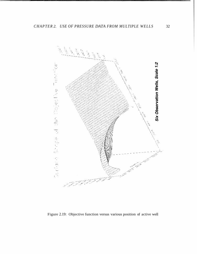
Example 1: Unknowns kz, r’, O’, a, ctZ, C Table 2.3 includes the pressure data generated with one percent noise and the
known reservoir properties used are shown in Table 2.4. The initial guess and the

C H A P T E R 2. USE OF PRESSURE DATA FROM MULTIPLE WELLS
Table 2.3: Generated pressure data for the reservoir of Example 1 I Active Well 11 Observation Wells 1
Positions (x, y) I (0, 100) I (0, -100) I (100, 0) I (-100, 0) 1
36
C H A P T E R 2. USE OF PRESSURE DATA FROM MULTIPLE W E L L S
Active well At; APi
1.9953 48.7194
Observation Wells 1
at; APi APi APi APi 9.5499 10.9054 12.3914 12.2931 12.3826
I I I I I 1 2.5119 I 55.2196 11 10.9648 I 11.9544 I 13.5561 I 13.4564 I 13.5806 I 3.1623 3.9811
61.6283 12.5893 13.0069 14.6518 14.5340 14.6424 67.2365 14.4544 14.0602 15.7939 15.6419 15.7799
Table 2.4: Properties of the reservoir in Example 1 , Q
110 bbl/day 4 ru, p h Ct 1
0.3 0.4 f t 3.0 30 f t 50 rnd 8.e-6 l /psi
37

C H A P T E R 2. USE OF PRESSURE DATA FROM MULTIPLE WELLS 38
Table 2.5: Initial guess, matching result and true value
Initial Guess IC2 md r' ft 8' a f t ct2 ( l l p s i ) C (bb l lp s i )
50 50 50 50 8. x .05 Matching Result
True Values
matching result are listed in Table 2.5. The matching started from the initial guess
of a homogeneous model k l = k2 = 50(rnd) and ctl = ct2 = 8 x 10⁻⁶(l/psi). The
residual of weighted squares was 0.357 and iteration number reached 40 to achieve
the absolute and relative errors for each parameter less than In this example,
there is one observation well located in the discontinuity and the noise is only one
percent, so the result is encouraging. However if kl and ctl were unknown, the initial
guess ICl = k2 = r' = a = 8' = 70, ctl = ct2 = 1. x C = 0.05 resulted in
incorrect estimated values of IC, = 159, IC2 = 104, r' = 83, 0' = 125, a = 58, ctl =
10.4 x
Example 2: Unknowns k l , k2, r', 8', a , ct l , ct2, C ct2 = 11.2 x C = 0.1 with the residual 38.0 after 11 iterations.
This example also has one observation well located in the discontinuity region,
and the noise added in pressure data is 3 percent.
Table 2.6 and Table 2.7 include the pressure data and the property data of the
reservoir, respectively. The initial guess, matching result and the true parameter
values are shown in Table 2.8. The absolute and relative errors of each parameter
are wit,hin lo-' after 14 iterations, which gives 1.94 as the residual of the weighted
squares.
J. 110.0 79.8 81.5 49.1 1l.E-6 0.0998 110 80 80 50 11 .E-6 .1
2.2.6 A Special Case - Concentric Active Well
If r' = 0, the active well is concentrically located in the discontinuous region. The
pressure drop in Laplace space can be simplified to be

C H A P T E R 2. USE OF PRESSURE DATA FROM MULTIPLE WELLS
Active Well
39
Observation Wells ,I
Positions (x, y) I (0, 100) 1 (0, -100) 1 (100, 0) I (-100,O)

C H A P T E R 2. USE OF PRESSURE DATA FROM MULTIPLE WELLS
Active Well At; AP;
1.5849 15.1704 1.9953 18.3564 2.5119 22.4510
Observation Wells At; A P; A P; AP; A P;
8.3176 5.6226 5.7772 5.5340 6.4860 9.5499 6.6476 6.7930 6.6091 7.7252
10.9648 7.7459 7.9858 7.7805 9.1468 3.1623 3.9811
27.3059 12.5893 8.9455 9.1699 8.9129 10.4160 32.2894 14.4544 10.2400 10.5519 10.2032 11.9558
Table 2.8: Initial guess, matching result and true value
q bbllday 110.0000
porosity rw f t viscosity thickness 0.3000 0.4000 3.0000 30.0000
Initial
40
ICl md IC2 md r ' f t 8" a f t ctl ct2 l/psi C 50 50 50 50 50 5.E-6 5.E-6 .1
Match True
238.66 100.35 79.51 197.63 61.02 l8.6E-6 10.E-6 0.4 250 100 80 200 60 19.E-6 10.E-6 .4

C H A P T E R 2. USE OF PRESSURE DATA FROM MULTIPLE WELLS 41
From the approximate expressions for modified Bessel functions of small arguments:
A1 M -, A1 Xlazl . (-Znaz2) + A2az2 1 1 X2
So for small radius a and large time (small z ) , the pressure drop becomes
(2.27)
(2.28)
(2.29)
and its Laplace transforrnation inversion is easy to obtain. From Eq. 2.29, it can be
seen that the pressure drop outside the discontinuity is the same as the line source
solution (exponential integral solution) and the pressure drop inside discontinuity should be the line source solution plus 141.2 k:h B p 2 ( & - 1) In :. Therefore, a composite
reservoir with a centered source well can be treated in convention as a homogeneous
reservoir without the first region by introducing a skin factor
A2 n s = (- - 1)Zn-. A1 r
(2.30)
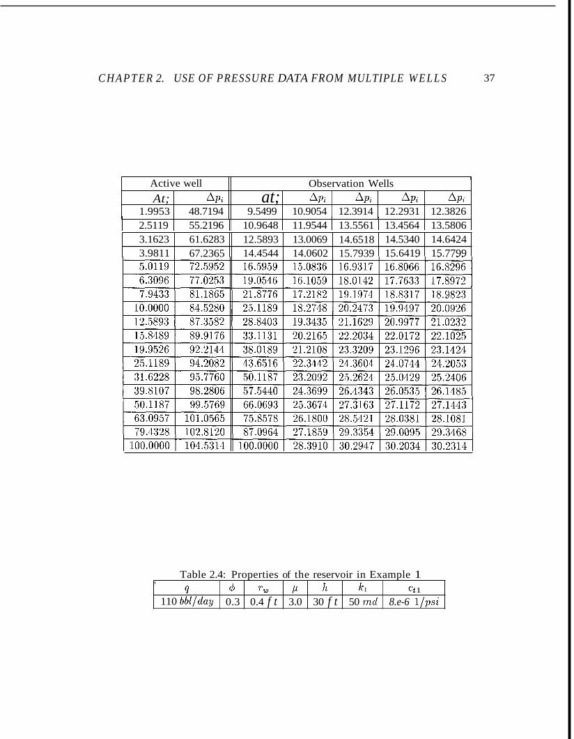
However, this simplification is true only when the radius of the first region is not very
large and the time considered is not very small. Fig. 2.21 and Fig. 2.22 provide an
idea what a and t should be. For a = 50 ( f e e t ) , t 5 1 (hour), using the skin factor
approach will result in incorrect results as shown in Fig. 2.21.
C H A P T E R 2. USE OF PRESSURE DATA FROM MULTIPLE W E L L S
I I I I I I I I I I I I I I I I I I I I I I I I I I 1 1 1 1 I I I I
-0 0
8 s i
8 i3
(aJnSSaJd) d
42
Figure 2.21: Comparison of pressure responses between skin factor approach and discontinuity approach

C H A P T E R 2. USE OF PRESSURE DATA FROM MULTIPLE WELLS 43
Figure 2.22: Comparison of pressure responses between skin factor approch and dis- continuity model approach
C H A P T E R 2. USE OF PRESSURE DATA FROM MULTIPLE WELLS 44
0
s s o - 3 3
0 0
8 8 8 0 8 - alnssald
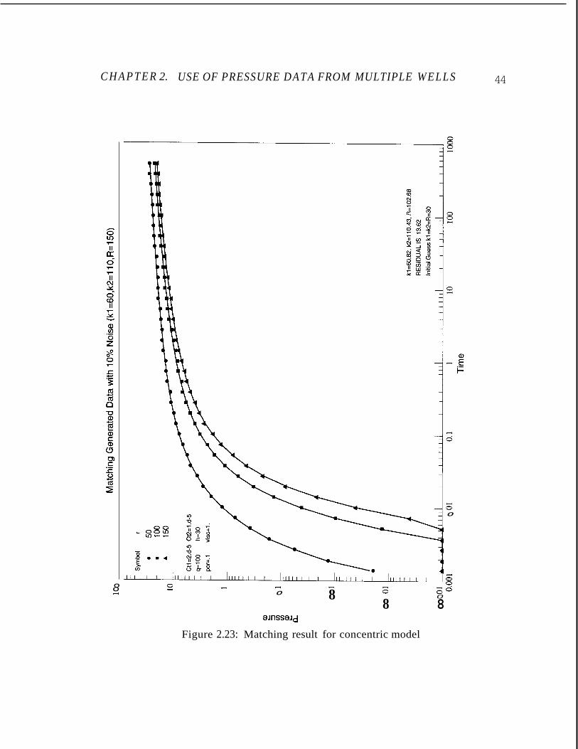
Figure 2.23: Matching result for concentric model

C H A P T E R 2. USE OF PRESSURE DATA FROM MULTIPLE WELLS 45
alnssaJd
Figure 2.24: Matching result for concentric model

C H A P T E R 2. USE OF PRESSURE DATA FROM MULTIPLE W E L L S 46
The same thing happens in Fig. 2.22 where a = 100 feet, t 5 10 hours. For the
general concentric composite reservoir where the simplified skin factor approach does
not apply, the solution presented in Eq. 2.26 runs faster and is more suitable than
the solution presented in Eqs. 2.10 and 2.11 in finding the unknown parameters such
as ICl, k2 and a as shown in Fig. 2.23 and Fig. 2.24.
In summary, for circular discontinuities, parameters such as permeability, com-
pressibility in both regions can be obtained in addition to the location and the range
of the discontinuous region if the noise in the pressure data are not large. The more
data that are used, the higher tolerance for noise that may be allowed in pressure
data for parameter identification. The wellbore storage coefficient in the active well
can also be estimated. If the active well is located in the center of the discontinuous
region, a skin factor may replace an explicit representation of the discontinuous region
under some restrictions.

C H A P T E R 2. USE OF PRESSURE DATA FROM MULTIPLE WELLS 47
2.3 Analysis of Drawdown-Buildup Pressure Data in Multiwell Systems
This section focuses on how the producing neighbor wells affect the buildup pressure
data in the testing well. The investigation started with the development of the so-
lutions in Laplace space and covered the system of both finite number of wells and
infinite number of wells. The system of an infinite number of wells can be used to
simulate the behavior of transient pressure in rectangular reservoirs.
Consider an infinite homogeneous reservoir with n + 1 wells. All wells are labeled
with an integer. Well 0 is the observation well, well 1 is the testing well producing
at a constant flow rate q at the beginning and at constant rate 0 after t p D , while
wells n ( n > 1) are the neighbor wells producing at constant rate q at any time.
The producing neighbor wells in this configuration will have impact on the pressure
buildup on the observation well. The pressure data from shut-in test of well 1 cannot
be analyzed correctly without studying the effect of neighbor wells.
If the wellbore storage effect is taken into account, the pressure solution in Laplace
space for the multiwell system of finite number of wells can be obtained by superposing
finite sources in time and space,
or basing the time scale on and using as the parameter, T e D T e D
(2.32)
where CD is the wellbore storage coefficient, and r;D is the distance between obser-
vation well 0 and well i.
T,D [ ( I - - e -P tpD "ZD )KO ( T I D f i / T e D ) + K O ( T 2 D f i / T e D ) + l c O ( T g D f i / T e D ) + d k b (TnD f i / T e D ) l
z' (K1 ( f i / r e D ) + C D f i / r e D ~ O ( J F / T e D ) )
When n = 1, this solution represents the interference case with one active well
and one observation well in an infinite homogeneous reservoir. The type curves for

C H A P T E R 2. USE OF PRESSURE DATA FROM MULTIPLE WELLS
1. i \
1. , \* '.
\ \
\. \ \. \ \
\. \ \. \ \. \ \
\. \ \. - - - _ _
\. \. .................................. \.
\, ..... .... \. ... \. \. \. \.
*- --. - _ /--% --
'%._
10 100 1000 1C 1
Drawdown and Buildup Type Curve (finite source) 10
Line TpOIrO2 .04 .4 ..............
10
1.
0 n
0.1
0.01
TD/rD2
Figure 2.25: Interference pressure response versus production time
Drawdown and Buildup Type Curve (finite source)
Line TpOIrDP
.04
.4 .............. I . 10. 100. 1000. 6000.
- - - - - - - ----
- ._ ._ .-
CD=10. rD=l .
48
I00
100

C H A P T E R 2. USE O F PRESSURE DATA FROM MULTIPLE WELLS
Drawdown and Buildup Type Curve (finite source) 10 Line TpDIrD2
.04
.4 ,_ ._ .- .- .- I .
IO. 100.
6000.
- .- __.__-. r .- '- \
1000. /--:- !. ,' I
I
__-.--- _- I \
49
Figure 2.27: Pressure response versus production time and wellbore storage effect
Drawdown and Buildup Type Curve (finite source) 10
Line TpDIrD2 .04 .4 ..............

C H A P T E R 2. USE OF PRESSURE DATA FROM MULTIPLE W E L L S 50
drawdown and buildup without wellbore storage are provided by Ramey (1981) as
shown in Fig. 2.25. In this special case, the pressures at any place are the same
except at early time if p D is plotted vs. 9 with !.e as a parameter (reo = r lD = ro) . As can be seen from Fig. 2.26, Fig. 2.27 and Fig. 2.28, the pressure responses depend
greatly on the distance between testing well and observation well if wellbore storage
is considered.
T D T:,
Fig. 2.29 and Fig. 2.30 show the pressure drawdown and buildup for a six-well
system, where the testing well is also the observation well. All the production wells
contribute to the drawdown curve. When the testing well is shut in, the buildup curve
eventually follows the curve corresponding to the production of all the neighboring
wells.
Fig. 2.31 and Fig. 2.32 show the buildup parts for the same system. For a fixed
shut-in time, p D will become larger than p ( t p D ) at late time, so each curve reaches
below zero at some time. The shut-in time affects the buildup pressure data very
much as well as the wellbore storage effect as can be seen from Fig. 2.31.
If there are infinite number of wells, well 0 is the observation well, well 1 is the
testing well producing at constant rate q first and at constant rate 0 after t p D , if all
the other neighboring wells are producing at the constant rate q all the time, and if
the wellbore storage effect is included, the pressure solution in Laplace space for the
infinite system can be written as
(2.33)
where r , ~ is the distance between observation well 0 and well n.
To compare the effect of number of wells on the drawdown and buildup curves,
a six-well system and an infinite-well system shown in Fig 2.33 are considered as
an example, where the distances in x direction and y direction between any two
neighboring wells are 5 0 0 f t , and the testing well and observation well are located at (0,O). 'The pressure response due to the production of infinite neighboring wells is

C H A P T E R 2. USE OF PRESSURE DATA FROM MULTIPLE WELLS
i
- Llne TpWRalRe
0.4 1. 10. 100.
.............. - - - - - - - - - _ _
~ Line TpDlRelRe
0.4 1. 10. 100.
.............. - - - - - - - - - _ _
- - __ .- .- .- i __.- .- .-. 1000.
10000. -_-.- !
- - 10 60000. - -
- - -
-
-
0 1. - a
0.1 ~~
0.01 I I I , , , , , , I 1 0.1
TDIRelRe
Figure 2.29: Pressure response versus production time
51

C H A P T E R 2. USE OF PRESSURE DATA FROM MULTIPLE W E L L S
0.1 0.01
10
B a 1
I . . i : I i : I I I I I I I , , , I , , , , , , , , I , , , , , , , , I
CD=100.0 I R e = 1 0 0 :, ,. , , , b
10 100 1000 11 0.1 1.
n a
B 2 a
Buildup Type Curve for Six-Well System (finite source)
Line TpDIRelRe
Buildup Type Curve for Six-Well System (finite source) 10
Line TpDIRelRe 0.4 1 . 10. 100. 1000.
. .. . . .. . . .. . . .
10000.
\ : I ! : I : : I ! : I : : I : : I ; : I
Testing Well at (0.0, 0.0) Obsers Well at (0.0. 0.0)
CD=O.O : I
I I , I I , , , , I , , , / , , , , I , , ~ , , _ , / , 1 , , 1 , , , , , 1. 10 100 1000 1(
: . I : I
I Re=100 0.1 0.01 0.1
(TD-TpD)/Re/Re Figure 2.32: Pressure buildup versus time after shut-in and wellbore storage
52
00
100
effect

C H A P T E R 2. USE OF PRESSURE DATA FROM MULTIPLE WELLS
Six-well Svstem
53
Infinite-well Svstem
Figure 2.33: Configuration of six-well and infinite-well systems
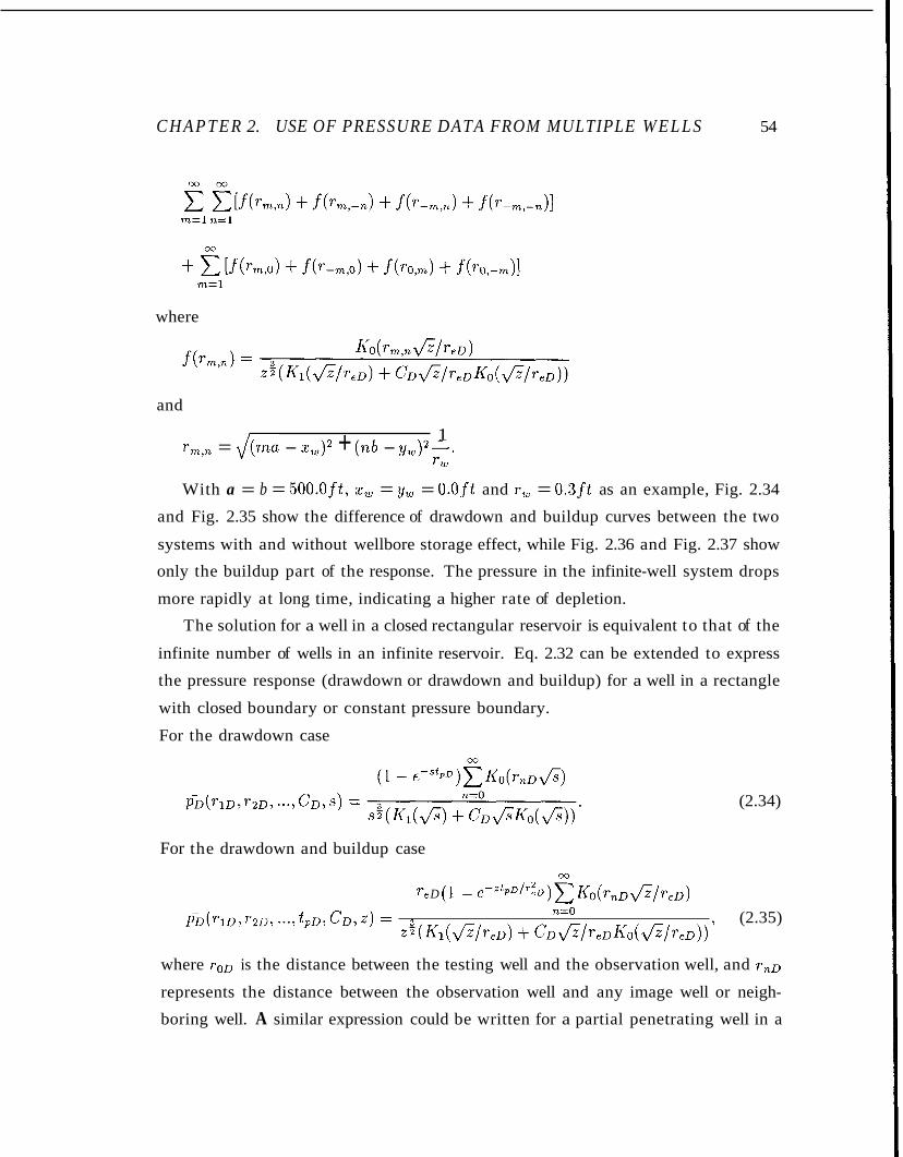
C H A P T E R 2. USE OF PRESSURE DATA FROM MULTIPLE WELLS 54
m = l n=l
where
and
1 rW
r,,, = &na - 2, )2 + (nb - y,)2-.
With a = b = 500.0ft, z, = yw = 0.Oft and r , = 0.3ft as an example, Fig. 2.34
and Fig. 2.35 show the difference of drawdown and buildup curves between the two
systems with and without wellbore storage effect, while Fig. 2.36 and Fig. 2.37 show
only the buildup part of the response. The pressure in the infinite-well system drops
more rapidly at long time, indicating a higher rate of depletion.
The solution for a well in a closed rectangular reservoir is equivalent to that of the
infinite number of wells in an infinite reservoir. Eq. 2.32 can be extended to express
the pressure response (drawdown or drawdown and buildup) for a well in a rectangle
with closed boundary or constant pressure boundary.
For the drawdown case
(2.34)
For the drawdown and buildup case 00
re D (1 - e - Z t p D / ' a D ) C I ( o ( r n O & / l ' e ~ ) (2.35)
where roD is the distance between the testing well and the observation well, and r,D
represents the distance between the observation well and any image well or neigh-
boring well. A similar expression could be written for a partial penetrating well in a
n=O p % ( r l D , r2D1 .-*, tpDi C D , *) =
z ' ( I ( l ( & / r e D ) + c D & / T e D I < O ( f i / r e D ) ) )

C H A P T E R 2. USE OF PRESSURE DATA FROM MULTIPLE WELLS
Drawdown-Buildups for Six-Well System and Infinite System (finite source) 1 02
Line TpDIRe/Re Well
10. Six 100. Six 10. Infinite 100. Infinite
..............
Testing Well at (0.0. 0.0) Obsers Well at (0.0, 0.0)
CD=O.O &=I00 I I , , , , , , , I / , , , , , , , 1 , , , , , , , , j , , , , , ( , , 1 / , , , , , , 10-2
1 10-1 10 TDIRelRe
Figure 2.34: Pressure response versus production time
Drawdown-Buildups for Six-Well System and Infinite System (finite source) 1 0 2
/' /
- Llne TpD/Re/Re Well
/ 10. Six 100. Six
100. Infinite /
.............. //
/ - - - - - - - 10. Infinite ---- /
55
Testing Well at (0.0. 0.0) k Ob& well at i0.0. o.oj
CD=100.0 Re=100 I I , 1 I , , , / I 1 , 1 , , / , , I , , , , , , , , 1 , , , , , , , , 1 , , , , , 10-2
10'' 1 10 TDIRelRe
Figure 2.35: Pressure response versus production time and wellbore storage effect

C H A P T E R 2. USE OF PRESSURE DATA FROM MULTIPLE WELLS
- - Llne TpDIRWRe Well - 10. Six 100. Six ..............
- - - - - - - 10. Infinite _ - _ _ 100. Infinite
- - - Llne TpDlRWRe Well
- 10. Six .............. 100. Six - - - - - - - 10. Infinite - - _ _ 100. Infinite
1
10-1
10-2
I I I I , I I I , , , I , , , , / , , , I , I , , , , , , / I , i , , , , , ,
CD=O.O Re=100
10-2 10-2 10.’ 1 10
TDIRelRe
L I
Testing Well at (0.0, 0.0) Obsers Well at (0.0, 0.0)
I I I I I I I
I I I I I I I I I l I I 1 1 1 I I I I ( I 1 1 1 I ! , , , , / I 1 , , , , , , : , , CD=lM).O R e = l 00
Figure 2.36: Pressure buildup response versus time after shut-in
56
effect

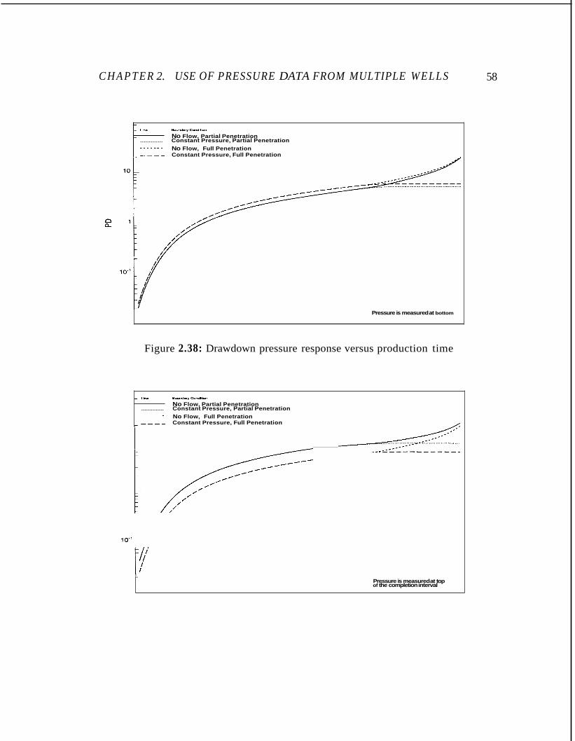
C H A P T E R 2. USE OF PRESSURE DATA FROM MULTIPLE WELLS 57
reservoir with no flow or constant pressure boundary where superposition by imaging
is applicable. As an example, the pressure responses are calculated in Fig. 2.38 and
Fig. 2.39 for a rectangular reservoir of 800ft x 5 0 0 f t , thickness sof t , permeability
lOOmd in radial direction and z direction. The testing well and observation well are
located at (looft, 1 0 0 f t ) with well radius 0.3ft. The well penetrates the upper 60%
of the formation thickness and the pressure is measured both at the bottom of the
well and at the top of the completion interval. The difference in pressure responses
between the partial penetration and full penetration is noticeable in Fig. 2.38 and
Fig. 2.39 from early time through late time. In well test analysis, if the partial pene-
tration effect is not considered, the permeability of the reservoir will not be correctly
interpreted.
C H A P T E R 2. USE OF PRESSURE DATA FROM MULTIPLE WELLS
- L,"* Boumlw C-llon
- No Flow, Partial Penetration ............. Constant Pressure, Partial Penetration
No Flow, Full Penetration - - _ _ Constant Pressure, Full Penetration - - - - -.
Pressure is measured at bottom
- La". e0um.w -"ion
No Flow, Partial Penetration ~ .............. Constant Pressure, Partial Penetration
No Flow, Full Penetration _ _ _ _ Constant Pressure, Full Penetration - - - - - - - - 7
Figure 2.38: Drawdown pressure response versus production time
Pressure is measured at top of the completion interval
lo-'
L
58

C H A P T E R 2. USE OF PRESSURE DATA FROM MULTIPLE WELLS 59
2.4 No-Flow Linear Boundary
For an infinite homogeneous reservoir with a linear no-flow boundary of infinite length,
one method of locating the no-flow boundary is the Inference Ellipse method devel-
oped by Vela (1977). The Inference Ellipse method requires exactly two sets of
interference data to determine the position of the no-flow boundary. If more than
two sets of well pressure data are collected, as in most interference testing, using the
inference ellipse method can only provide rough estimates about the location of the
no-flow boundary and the result depends on which two sets of data are chosen. In this section, the pressure expression is formulated in consideration of applying multiple
sets of the pressure data to locate the no-flow boundary position. The approach will be applied to the field pressure data in following section.
If the wellbore storage effect is included at the active well, the pressure solution
in Laplace space would be
(2.36)
Consider a reservoir configured as in Fig. 2.40, where one active well and three
observation wells are present. The shapes of the least square residual objective func-
tion are shown in Fig. 2.41 and Fig. 2.42. Pressure data from two wells are used in
Fig. 2.41 and the objective function has two local minima, leaving the interpretation
result nonunique. However, if more than two sets of pressure data are used, there
will be only one global minimum as in Fig. 2.42. This indicates that using multiwell
interference pressure data simultaneously is necessary in locating the position of the
no-flow boundary as well as in estimating permeability and storativity. The wellbore
storage in the interference test is not important except when C D / r i becomes larger
than 10. It can be seen from Eq. 2.36 that small r D will contribute to the enlargement
of the wellbore storage effect.

60 C H A P T E R 2. USE OF PRESSURE DATA FROM MULTIPLE WELLS
Infinite linear no-flow boundaq
0 (50,551
't Observation well
0 (50, -55)
Figure 2.40: Well pattern for an infinite reservoir with a linear no-flow boundary

C H A P T E R 2. USE OF PRESSURE DATA FROM MULTIPLE WELLS 61
Figure 2.41: Contour of objective function using two sets of pressure data

C H A P T E R 2. USE OF PRESSURE DATA FROM MULTIPLE WELLS 62
t
L
t
Fi,gure 2.42: Contour of objective function using three sets of pressure data

C H A P T E R 2. USE OF PRESSURE DATA FROM MULTIPLE WELLS 63
2.5 Interpreting Multiwell Pressure Data of Ohaaki Geothermal Field
This section shows the interpretation of a set of interference data from Ohaaki geother-
mal field using nonlinear regression. Multiple sets of pressure data were used. The
purpose was to identify how the no-flow boundary affects the result.
Using interference testing to evaluate reservoir heterogeneity and average trans-
missivity and storativity is a convenient and common method in geothermal fields.
Twelve interference tests were conducted in the Ohaaki geothermal field among six
wells at different times. Leawer et al (1988) analyzed these tests in an effort to iden-
tify a no-flow linear boundary using the inference ellipse method by Vela (1977). The
pressure data sets were matched only one pair at a time. The results were dominated
by the local transmissivity and storativity between or around the two wells; each
match gave a different local average. It is hard to determine which value can be used
as the average for the whole reservoir. Furthermore, the inference ellipse method
carries some uncertainty in deciding the location of linear boundary, since two pairs
of data provide two inference ellipses that are sufficient to determine the location of
linear boundary. A better approach is to match all the pairs simultaneously to give
consistent results.
The parameters matched were bulk transmissivity k h / p , storativity $cth, the lo-
cation of linear boundary (two coordinate variables) and the initial pressures of each
active well. There are twelve sets of interference pressure data available, which means
we have sixteen parameters to be matched in our model. The theoretical drawdown
and buildup curves used in our analysis were similar to those developed by Eip- p e r (1985), but the linear boundary effect has been included in the curves in order to
regress on all the parameters together. To make this possible, a Cartesian coordinate
was created with BR20 as the origin, so the location of each well is represented by a
pair of numbers (x, y) as follows:
BR23 (0.0, 0.0)
BR13 (-1079.9, -1977.3)
BR23 (-527, -1230.31)

C H A P T E R 2. USE OF PRESSURE DATA FROM MULTIPLE W E L L S 64
BR3I (-1757.5, -878.8)
BR34 (-2680.3 , -2636.4) BRl9 (-1318, -659.1)
We represented the linear boundary by another pair of ( x , y ) , the coordinates of one
point on the boundary that are nearest to the origin of our Cartesian coordinates.
The algorithm used to solve this nonlinear regression problem is the same modified Fletcher (1971) method discussed in Section 2.2.4.
The results from Leaver et aZ(1988) are presented in Fig. 2.43 and listed as follows with ail average set of values:
kh. = 250.0 d ft $cth = 80.0 ft/psi X lo4 xb = -1494.0 f t Y b = 2724.0 ft,
This interpretation gives a residual of 1.999 psi2 per data point (there are 1969 data
points for all 12 wells). Starting from this result as an initial guess, after 11 iterations,
the algorithm found a solution as shown in Fig. 2.44:
kh. = 547.92477 $cth = 119.91531 xb = -1981.07651 Y b = -1631.12899,
which gave an average residual of 1.4366 psi2 per point. Notice that tests B 7 and
B8 are worse than before, because they have fewer points and contribute less to the
residual.
Adding the twelve initial pressures of the active wells as parameters, we were able
to reduce the residual to 0.97 psi2 per data point as shown in Fig. 2.45 with estimated parameter values as follows:
kh. = 584.96150 $cth = 47.34690 xb = -3031.12267, Y b = -2076.63377
p:’ = -7.11689 pB2 = -10.50041 pB3 = -53.15206 pr4 = 14.30722
$6 = -9.13517 pB7 = -117.83430 pB8 = -67.89931 pB9 = 297.20062
p;lo = -32.76060 pC’ = 3.36854 p f 2 = -24.25505 pC3 = -6.17686
From Fig. 2.45, we see that four sets of data B6, B7, B8 and B9 are not well- behaved. Excluding these four sets, we performed the matching again with the re- maining eight sets of pressure data. Fig. 2.46 is the matching result without initial pressures as parameters but with weights to emphasize the early data. The result is

C H A P T E R 2. USE OF' PRESSURE D A T A FROM MULTIPLE W E L L S 65
k h = 734.75503 &th = 52.16619 x b = -1663.09485 t j b = -2883.21636
With initial pressures as parameters without emphasis on early data, we have (Fig. 2.47):
kh, = 659.31439 q!qh = 32.35258 xb = -5067.12074 t j b = 18.74405 pF1 = -4.88181 pB2 = -2.75039 pB3 = -54.73846 pB4 = 14.38455 pBlo = -29.48337 p f 3 = 14.83868 p; c1 - - 12.12687 py2 = -14.24363
With weights and initial pressures as parameters, we end up with
kh, = 630.98879 &h = 33.71702 X b = -1506.85394 Y b = 2749.59898 p f 1 = -4.41652 p f 2 = 0.37996 p;3 = -61.96414 pZB4 = 17.10718 pB10 = -34.01868 p f " = 5.96005 p f 2 = -28.81102 pC3 = 17.35140
as shown in Fig. 2.48. All the results were calculated with h = 2297.0 f t and p =
0.34 cp. Notice that in B3 of Fig. 2.46 we see the calculated type curve parallel above
the actual data and we can not shift the curve vertically without sacrificing other
matches. All the data affect each other here. When the initial pressures are allowed
to vary, the actual data of B 3 are increased by the same amount, resulting in the
early data having a big jump in the log-log graphs as in Fig. 2.47 and Fig. 2.46. The location of the linear boundary is sensitive to the sets of data used. It is more
likely that there is a northwest/southeast trend of faults, and we always had a higher
estimate of average permeability than the value 110 rnd as suggested by Leaver et
al (1988).

CHAPTER 2. USE OF PRESSURE DATA FROM MULTIPLE WELLS
I
D
P
I I
dV dV
66
Figure 2.43: Approximate matching results from Leaver et al (1988)

CHAPTER 2. USE OF PRESSURE DATA FROM MULTIPLE WELLS 67
d0
I
I
- 4 dV
Figure 2.44: Matching results without weights and initial pressures as parameters

C H A P T E R 2. USE OF PRESSURE DATA FROM MULTIPLE WELLS
1 I 1 I I 1
dV dV dV
68
Figure 2.45: Matching results with initial pressures as parameters
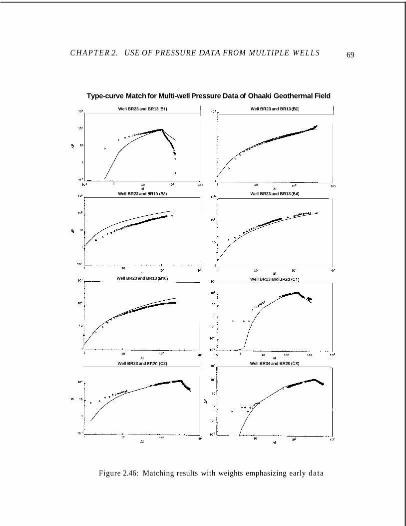
C H A P T E R 2. USE OF PRESSURE DATA FROM MULTIPLE WELLS
l0-l
1 02
% 10
1
10-1
Type-curve Match for Multi-well Pressure Data of Ohaaki Geothermal Field
Well BR23 and BR13 (Bl) , 103 ~ Well BR23 and BR13 (82) ,
I - , , . . , . 1
J 1 1 102 1 03 lo-' 10 102 1 03 10
AI Ai ~
10-1 ~ Well BR23 and BR19 (83) ~ ~ Well BR23 and BR13 (84)
1 0 - l L , , 1 I , , , , , , , , , , , , . I , , , , , , . L I 1
1
102 103 1 10 102 103 10
Ai AI _. Well BR13 and BR20 (Cl) Id
Well BR23 and BR13 (B10)
1 1 103 10.1 10 102 103 le 10 102
Well BR23 and BR20 (C2) , ld ~ Well BR34 and BR20 (C3) AI AI
a
69
Figure 2.46: Matching results with weights emphasizing early data

C H A P T E R 2. USE OF PRESSURE DATA FROM MULTIPLE W E L L S
1 . _
Type-curve Match for Multi-well Pressure Data of Ohaaki Geothermal Field
~ Well BR23 and BR13 (Bl) , 103 ~ Well BR23 and BR13 (82)
102 ~
10 ~
a -
1 -
10' =
1 0 2 I , ,
10 102 103 1 1 10 102 103
At At 103 Well BR23 and BR13 (Blo) , ~ Well BR13 and BR20 (Cl) ,
lol ~ Well ER23 and BR20 (C2) , ~ Well BR34 and BR20 (C3)
1 1
io3 , I 10-++L!.........,......
102 1 o3 10 1 02 10
At At
70
Figure 2.47: Matching results with initial pressures as parameters

C H A P T E R 2. USE OF PRESSURE DATA FROM MULTIPLE W E L L S 71
I ype-curve Match tor Multi-well Pressure Data of Ohaaki Geothermal Field
1 03
lo2
% 10
1
10'
Well BR23 and BR13 fB1)
l e
1 02
n
10
1
I d
102
a
10
1
At Well BR23 and BR19 (83)
~
Well BR23 and BR13 (82)
1 1 1 0 102 103
At Well BR23 and BR13 (84)
lo3 9
" * t
lo" 103 1 1 0 1 02 103 10 102
At A1
---I 10ZFA-l
1 0 lo2 I d 104 10 102 103 10-1 At At
loJ ~ Well BR23 and BR20 (C2) , 103 E Well BR34 and BR20 (C3) ,
Figure 2.48: Matching resul s with weights and initial pressures as parameters

Chapter 3
Green’s Fun(
Reciprocity 1 Heterogeneo
This chapter starts with the
reservoirs and the discussion c
pressure in terms of Green’s f shown that the Green’s functi
pressure solutions for heteroger
product property.
The Principle of reciprocit]
skin on reciprocity is also incl
problems is briefly discussed.
3.1 Definition of
For pressure transient calculat
is usually defined as the pressui
point source of unit strength gt
being initially at a constant p
tions and the
’rinciple in
ILS Media
efinition of the Green’s function for heterogeneous
its properties. The general expression to represent
nctions is presented. Through some examples, it is
n method is still a helpful tool in finding analytical
ous reservoirs even though it loses the useful Newman
is discussed next. The effect of wellbore storage and
ded. Finally, using Green’s functions in tracer flow
Green’s Functions
ns in a homogeneous formation, the Green’s function
response at (z, y , z ) at time t due to an instantaneous
.erated at point (z’, y’, z’) at time 7, with the reservoir
mure p;, and the boundary being kept without flow
72

C H A P T E R 4. GREEN’S FUNETION AND RECIPROCITY PRINCIPLE 73
or at the same constant pressurb pi. So, the Green’s function G ( x , y, z , x’, y’, z’, t - T )
is the solution to the following Jequation,
( 3 4
( 3 4
d2G d2G + - = d2G *dG - + a y z d z 2 ~ k d t d X 2
--
G(z, y, Z , z’, y’, z’, 0) = S(z i x’)S(y - y’)S(z - z’)
where S(x) is the Dirac functjon, which is handled algebraically as if it were an
ordinary function with the following properties,
S ( x ) = 0 for 2 # 0
J--00
and
for every arbitrary continuous tipnction #(x). However this definition of Green’s func-
tion can not be used directly fo$ heterogeneous reservoirs, since the coefficients of the
flow equation for heterogeneous reservoir are not constant.
There are two ways to defide the Green’s function for heterogeneous formations.
One treats the instantaneous source still as an initial condition and the time range
involved is [0, m]: I
I
- d k ( ~ , y , z ) -+--+-+- dG d k(z ,y , z ) dG d k(z ,y , z ) dG dx’:(z,y,z) b ( z , y , z ) dz’:(”,Y,z)ds
Another way treats the instantbneous source as a source with strength concentrated
at time T , the time range as (-~oo, m) and restricts the solution to be zero for t < T .
So G(x , y, z , z’, y’, z’, t - T ) is a~solution of the following equation:

CHAPTER 4. GREEN’S FUN
G ( x , y , z , d, y’, z l , t ) = 0 for
I C , p , $ and et above are a,ll func
or continuous within several s i
subdornains’ boundaries along
and material balance are maint
These two definitions are eq
functions from the first and thc
where
If G1 satisfies Eqs. 3.3 and 3.4,
+--) d kdGz = -(--) d kdG1 ax, /L d X i ax; p axi
so G:! satisfies Eqs. 3.5 and
understand and has more obvi’
as the pressure response due tc storativity at the source locati
the hoinogeneous case.
TION AND RECIPROCITY PRINCIPLE 74
- x’)S(y - y’)S(z - z‘)S(t - 7 ) ( 3 . 5 )
< 7. (3.6)
m s of (x, y, z ) , continuous throughout the reservoir,
‘domains of the reservoir and discontinuous on the
vhich additional conditions of continuous pressure
ined.
valent in some sense. Assume G1 and G2 are Green’s
second definitions respectively, then
‘l(2, Y, z , XI, Y1, z17 t - T ) H ( t - 7 ) (3.7)
i. We chose the first approach which is easier to
is physical meaning. It defines the Green’s function
%n instantaneous source of a strength related to the
1, rather than due to an always unit strength as in

C H A P T E R 4. GREEN’S FUNLTION A N D RECIPROCITY PRINCIPLE 75
3.2 Properties of( Green’s Functions
From the definition, some propbrties can be inferred for Green’s functions in hetero-
geneous reservoirs. Those propkrties will be applied to derive the expression for the
general pressure response in terms of Green’s function. I
1. Principle of reciprocity:
Proof is included in Appendix C. Once we have this reciprocity for a Green’s
function due to an insta taneous point source, it is not difficult to derive the
conditions of reciprocity $r the general pressure due to any kind of source. .I
2. G ( x , y, z , x‘, y’, z’, t - 7) a a function of (x’, y‘, z’, 7) satisfies: 1 d k ( z ’ , y‘, 2’) dG I & k(z’, y’, 2‘) dG
-t - dx’ p(x’, y’, 2’) dx’ y’ p ( d , y’, 2’) dy’
3. The initial condition give$:
(3.10)
(3.11)
4. IF the outer boundary of #amain 0 is closed or no-flow, then for t > 7: I s, $(x’, y‘, z ’ ) c t ( 4 y’, 4’)G(x,y, z , x’, Y’, Z’, t - 7)dR = 1 (3.12)
The Newman’s product thebrem presented by Newman (1936) does not hold in
heterogeneous reservoirs. This 1s a major limitation on the use of Green’s functions
for heterogeneous problems. ‘I/he Green’s functions have to be found individually,
instead of being constructed f T m existing easier solutions. This restriction comes
from the fact that the domain can not be decomposed as in the homogeneous case,
for instance, a cubic region (tbree-dimensional) is no longer the product of three
one-dimensional intervals.
I

C H A P T E R 4. GREEN'S FUNkTION AND RECIPROCITY PRINCIPLE 76
3.4.1 Case 1: Separaiion
3.3 Pressure in Terms of Green's Functions
of Variables
The Green's function is the pr ssure response due to an instantaneous point source
in the reservoir with homogen ous boundary conditions. With that, we can derive
the pressure response due to aby kind of source in the reservoir and with any non-
homogeneous boundary condition. Suppose that the distribution of pressure in the
1 I
reservoir is initially g ( x , y , z ) ,
( x , y , z ) , at time t with a unit
then the pressure can be
the source in the reservoir is f ( x , y , z , t ) at point
rate of injection per unit volume of reservoir,
terms of the Green's function:
(3.13)
The detailed derivation is inchbed in Appendix B.
3.4 Examples of Green's Functions
Without the Newman product n scheme it is more difficult to find the Green's func-
tion for a heterogeneous region] Appropriate mathematical method is needed for the
method to be successful in hetirogeneous reservoirs. In this section, several mathe-
matical methods are presented with examples in finding Green's functions for some
interesting and practical distri /I utions of permeability and porosity.
I
O < x < 1 , t > O d ,dG dG - (e -) = e"- a x d x at
6 ( x - d) ~
G ( x , x ' , ~ ) = ex' I
(3.14)
(3.15)

C H A P T E R 4. GREEN’S FUA
G(O,x’ , t ) = G ( l , x ’ , t ) = 0
The corresponding Sturm-Liou
d d X -(ez--) + X ezX = 0 dx dx
X ( 0 ) = X ( 1 ) = 0.
The equivalent equation
X” + X’ + AX = 0
gives
where C1, Ca and X are decide
1 4
n = 1,
with C‘1 = 0 and eigenfunction
2 2 X=-n r +-,
-(n2r2+1/4)t-: G,(z , t ) = Cne
Using the initial condition, mi
the Green’s function is: 00
~ ( z , 21, t ) = 2 e - e - t
With the approach of varia dimensional flow problems wit ities, where either could be sci
n = l
0 k ( x ) / p ( x ) = 1 - 2 2 , #(x
JTION A N D RECIPROCITY PRINCIPLE 77
t > 0.
ille problem is:
(3.16)
(3.17)
(3.18)
(3.19)
(3.20)
from the boundary condition (Eq. 3.18)’
7 a * * (3.21)
sin n r x (3.22)
tiplying by e: sin n r x , then Cn = 2e-f sin nrx’ , and
sin nrx’ sin n r x (3.23) -n2r2t
le separation, Green’s functions can be found for one- the following distributions of mobilities and storativ- ed by a constant:
= x in region [-I, 11.
7 t ( x ) = 1 in region [-1,1].
: x ) = e-z2 in region (--a, cm).

CHAPTER 4. GREEN'S FUN(CTI0N A N D RECIPROCITY PRINCIPLE 78
0 k ( n : ) / p ( x ) = (1 - n:)P-qfl+q, $(z )C t ( z ) = (1 - z)P-qx*-l where q 2 1, p - q 2 0 in region [-I, 11. I ,
Special functions are involved
boundary condition at a place
those solutions. Notice that we can not specify a
mobility vanishes.
3.4.2 Case 2: Fouried Transformation
When the eigenvalue problem r sulted from the separation of variables has a contin-
uous spectrum, Fourier transfo mation is a good choice.
Let us try to find the Green s function in a two-dimensional infinite reservoir with
a plane interface at z = 0 whic separates the reservoir into two regions with different
properties of storativity and m bility.
Assume that the mobility abd storativity are A, and ql respectively for the half space x > 0 and A 2 and q2 re pectively for the other half n: < 0. Without loss of
generality, the position of the i stantaneous source can be taken to be at ( n : ' , O ) .
li I h
The free space Green's func ion in Laplace space is
Assume in region 1 that G =
space we need to solve:
(3.24)
' ~ 1 + w and in region 2 that G = 'u, then in Laplace
d2eu d2W 2 - -- + ~ - z , w = o dz2 dy I
~
for x > o
with boundary conditions:
li1 -+ w = v a t x = O
(3.25)
(3.26)
(3.27)

C H A P T E R 4. GREEN’S FUNETION A N D RECIPROCITY PRINCIPLE 79
at x = 0 (3.28) du1 dw - + -) = x 2 - ax ax ax
I
where z1 = 6 and 22 = 6. ~
problem, which suggests that
theorem. An equivalent way is to use the Fourier transformation.
Separation of variables z a d y gives a continuous spectrum for this eigenvalue
Fourier integral replace the eigenfunction expansion i After Fourier transformatio :
(92 =
~- (s2 + z ~ > w = 0 8x2 ,
T‘ for x > 0
tu
I
with C = 0 when x -+ --oo we $ee that:
A and B can be decided by the/ boundary conditions:
Substituting U l = le gives 2 a - F l
so
(3.29)
(3.30)
(3.31)
(3.32)
(3.33)
(3.34)
(3.35)
(3.36)

C H A P T E R 4. GREEN’S FUN
for z :, 0, and
for z <: 0. In Laplace space, thl
G(s , y,z I , z ) = Jz /w G ( x T O
3.4.3 Case 3: Workir
For infinite reservoirs, working
spatial variables without worr?
There are effective numerical r
real space conveniently.
A good example is the prc
with a circular discontinuity in
is easier to work in Laplace sp
homogeneous Green’s function
perturbation; adding a to-be-d
homogeneous reservoir without
for region i ( i = 1 ,2 ) , where u;
properties as region i and w; is composite media for heat tram
the Green’s function was define
the Green’s function lose the r(
quite inconvenient when applie
function in Laplace space for t
TlON A N D RECIPROCITY PRINCIPLE
@ q ( Z + X ’ )
t 2;
-
- ; z’
I-) Green’s function is
, I C 1 , 2 ) cos(ys)ds
; in Laplace Space
80
(3.37)
(3.38)
(3.39)
L Laplace space is a good idea since we can focus on
ig about the time variable or the initial condition.
:thods that invert the solutions in Laplace space to
iure solution for an infinite homogeneous reservoir
roperties as shown in Fig. 2.5. For this problem, it
:e. In Laplace space, a function extended from the
3s obtained by Rosa (1991). The key idea is a kind of
ided function to the already known solution for the
le discontinuity. The solution is assumed to be u;+v;
the solution of homogeneous reservoir with the same
he function to be decided. This idea was applied to
:r by Carslaw and Jaeger (1959). In their approach,
due to a unit strength source. This definition makes
iprocity property in heterogeneous reservoirs, and is
to continuous sources. In our definition, the Green’s
! first region ( r < a) is

CHAPTER 4. GREEN’S FUN
For the second region ( r 2 a) ,
where
E o = 1,
E, = 2 ( n > O ) , A -h - / 11 ’
A 2 = 2, 71 = &)
7 2 = &% 21 = 6, 2 2 = 6, R‘! = r2 + - 2rr’ cos ( I3
R,, = A 2 z 2 IC, (21 a) IC;( 2 2 a ‘
an = A 2 . 2 1 ; ( . 2 . ) I n ( . 1 4 -
9,, = A1 21 IC,( z&;( 2,a)
Notice that the two equations
because Eq. 2.10 a,nd Eq. 2. discontinuity problem.
The pressure drop for a ca
TION AND RECIPROCITY PRINCIPLE 81
In ( z1 r ) cos (8 - 0’)
if a 2 r’ 21 r ) - cos (8 - 6’)
if a < r‘
is
p’) ICn ( 2 2 r ) cos (8 - 6’)
(3.40)
if a 5 r‘ 2 4 - cos (0 - e’)
(3.41)
if a > r‘
1‘) >
A1 21 IC; (21 a ) Iin (22a) ,
121 In ( 2 2 4 1 ; (21 a) ,
h 2 2 2 K ; ( Z 2 a ) I n ( Z l a ) .
sented above are different from Eq. 2.10 and Eq. 2.1 1 are not actually Green’s function for the circular
ant surface flow rate q in Laplace space is
) . (3.42)

CHAPTER 4. GREEN’S FUNbTION AND RECIPROCITY PRINCIPLE
I
where I
I
v 2 r > a - v(r, 8 , z ) =
3.4.4 Case 4: Decom
We do not have Newman’s pro
reservoirs, so generally we can
several lower dimensional pro1
special cases, for example, wheI and are functions of only one o
Consider a closed rectangulz
tivity varying linearly in the n:
function for this problem satisf
d dG d -[(ax + b)-] + -[(ax t d X a x a y
which, after transformation wit
X’ = ax + b
y’ = ay + c
t‘ = a2t
1 dG d2G aG - -
is equivalent to the following p
-- (x- ) + - - x a x d x dy2 dt
with 0 5 a 5 x 5 band 0 5 y
S(x - X I ) G(:c, x’, y, y’, 0 ) =
X
This two-dimensional probll
lems by assuming
Substituting into Eq. 3.45, we
)OS t ion
82
uct theorem for Green’s functions in heterogeneous
not decompose a higher dimensional problem into
ems that are easier to solve, except in some very
mobility and storativity have the same distributions
x , y or z .
* reservoir in two dimensions with mobility and stora-
direction only, as shown in Fig. 3.4.4. The Green’s
:S:
dG dG b)-] = ( a x + b)-
i any constant c,
aY at (3.43)
(3.44)
Dblem:
(3.45)
1.
(3.46)
m can be decomposed into two one-dimensional prob-
( Y - Y‘)
G2(Y, Y‘, 4. )btain two subproblems,