Introduction Model Example Equalisation Conclusions References Proof

Application of Inflow Control Devices toHeterogeneous Reservoirs

Andrei Bejan(joint work with Vasily Birchenko, Alexander Usnich, and David Davies)

ECMOR XII, Oxford, September 2010

Introduction Model Example Equalisation Conclusions References Proof

Advanced well completions: ICDs and ICVsIncreasing well-reservoir contact

advantages: drainage area, sweep efficiency and delayed wateror gas breakthrough, well productivity

challenges: drilling, completion and production (uneven inflowdistribution)

Inflow Control Devices and Interval Control Valves: methods of study

using well modelling software and simulators (from basicfunctionality to capturing the annular flow effect)

analytical models (still can play a role in (i) quick feasibilitystudies, e.g. screening ICD installation candidates; (ii)verification of numerical/simulation results; (iii) communicatingbest practices without referring to specific products)

We present an analytical model for quantifying the inflowequalisation effect of ICD applications in heterogeneous reservoirs.

Introduction Model Example Equalisation Conclusions References Proof

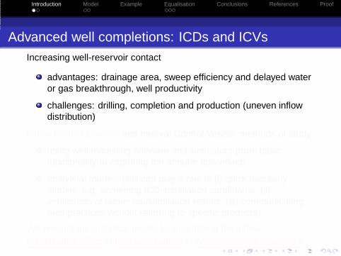
Advanced well completions: ICDs and ICVsIncreasing well-reservoir contact

advantages: drainage area, sweep efficiency and delayed wateror gas breakthrough, well productivity

challenges: drilling, completion and production (uneven inflowdistribution)

Inflow Control Devices and Interval Control Valves: methods of study

using well modelling software and simulators (from basicfunctionality to capturing the annular flow effect)

analytical models (still can play a role in (i) quick feasibilitystudies, e.g. screening ICD installation candidates; (ii)verification of numerical/simulation results; (iii) communicatingbest practices without referring to specific products)

We present an analytical model for quantifying the inflowequalisation effect of ICD applications in heterogeneous reservoirs.

Introduction Model Example Equalisation Conclusions References Proof

Advanced well completions: ICDs and ICVsIncreasing well-reservoir contact

advantages: drainage area, sweep efficiency and delayed wateror gas breakthrough, well productivity

challenges: drilling, completion and production (uneven inflowdistribution)

Inflow Control Devices and Interval Control Valves: methods of study

using well modelling software and simulators (from basicfunctionality to capturing the annular flow effect)

analytical models (still can play a role in (i) quick feasibilitystudies, e.g. screening ICD installation candidates; (ii)verification of numerical/simulation results; (iii) communicatingbest practices without referring to specific products)

We present an analytical model for quantifying the inflowequalisation effect of ICD applications in heterogeneous reservoirs.

Introduction Model Example Equalisation Conclusions References Proof

17

Courtesy Hulliburton

Courtesy Hulliburton

Introduction Model Example Equalisation Conclusions References Proof

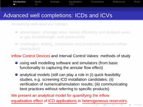
Model assumptionsflow through the reservoir can be described by Darcy’s law andthe inflow into the well is in steady or pseudo-steady state

distance between the well and reservoir boundary is muchlonger than the well length (or parallel to the well)

perpendicular-to-the-well components of the reservoir pressuregradients are much greater than the along-hole ones.

friction and acceleration pressure losses between the toe andthe heel are small compared to the drawdown (Birchenko et al (2010))

the fluid is incompressible

the completion interval does not need to be perfectly horizontal(hence TVD may vary along the completion)

no flow in the annulus parallel to the base pipe

ICDs installed are of the same strength

the flow distribution along the wellbore’s internal flow conduitq(ℓ) is smooth

Introduction Model Example Equalisation Conclusions References Proof

Model assumptionsflow through the reservoir can be described by Darcy’s law andthe inflow into the well is in steady or pseudo-steady state

distance between the well and reservoir boundary is muchlonger than the well length (or parallel to the well)

perpendicular-to-the-well components of the reservoir pressuregradients are much greater than the along-hole ones.

friction and acceleration pressure losses between the toe andthe heel are small compared to the drawdown (Birchenko et al (2010))

the fluid is incompressible

the completion interval does not need to be perfectly horizontal(hence TVD may vary along the completion)

no flow in the annulus parallel to the base pipe

ICDs installed are of the same strength

the flow distribution along the wellbore’s internal flow conduitq(ℓ) is smooth

Introduction Model Example Equalisation Conclusions References Proof

Model assumptionsflow through the reservoir can be described by Darcy’s law andthe inflow into the well is in steady or pseudo-steady state

distance between the well and reservoir boundary is muchlonger than the well length (or parallel to the well)

perpendicular-to-the-well components of the reservoir pressuregradients are much greater than the along-hole ones.

friction and acceleration pressure losses between the toe andthe heel are small compared to the drawdown (Birchenko et al (2010))

the fluid is incompressible

the completion interval does not need to be perfectly horizontal(hence TVD may vary along the completion)

no flow in the annulus parallel to the base pipe

ICDs installed are of the same strength

the flow distribution along the wellbore’s internal flow conduitq(ℓ) is smooth

Introduction Model Example Equalisation Conclusions References Proof

Specific inflow rate and specific productivity index:

U(ℓ) =dqdℓ

= j(ℓ)∆Pr = j(ℓ)(Pe(ℓ)− Pa(ℓ))

Model

∆P(ℓ) = ∆Pr (ℓ) + ∆PICD(ℓ) = U(ℓ)/j(ℓ) + aU2(ℓ), where

a =

(

ρcal µρµcal

)1/4ρ

ρcalℓ2

ICDB2aICD for channel ICDs,Cuρℓ

2ICDB2

C2d d4 for nozzle or orifice ICDs

Solution

qw =

∫ L

0U(ℓ)dℓ =

∫ L

0

−1 +√

1 + 4a∆P(ℓ)j2(ℓ)2aj(ℓ)

dℓ

Introduction Model Example Equalisation Conclusions References Proof

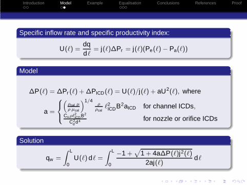
Specific inflow rate and specific productivity index:

U(ℓ) =dqdℓ

= j(ℓ)∆Pr = j(ℓ)(Pe(ℓ)− Pa(ℓ))

Model

∆P(ℓ) = ∆Pr (ℓ) + ∆PICD(ℓ) = U(ℓ)/j(ℓ) + aU2(ℓ), where

a =

(

ρcal µρµcal

)1/4ρ

ρcalℓ2

ICDB2aICD for channel ICDs,Cuρℓ

2ICDB2

C2d d4 for nozzle or orifice ICDs

Solution

qw =

∫ L

0U(ℓ)dℓ =

∫ L

0

−1 +√

1 + 4a∆P(ℓ)j2(ℓ)2aj(ℓ)

dℓ

Introduction Model Example Equalisation Conclusions References Proof

Specific inflow rate and specific productivity index:

U(ℓ) =dqdℓ

= j(ℓ)∆Pr = j(ℓ)(Pe(ℓ)− Pa(ℓ))

Model

∆P(ℓ) = ∆Pr (ℓ) + ∆PICD(ℓ) = U(ℓ)/j(ℓ) + aU2(ℓ), where

a =

(

ρcal µρµcal

)1/4ρ

ρcalℓ2

ICDB2aICD for channel ICDs,Cuρℓ

2ICDB2

C2d d4 for nozzle or orifice ICDs

Solution

qw =

∫ L

0U(ℓ)dℓ =

∫ L

0

−1 +√

1 + 4a∆P(ℓ)j2(ℓ)2aj(ℓ)

dℓ

Introduction Model Example Equalisation Conclusions References Proof

Inflow equalisation using ICD: an example

Introduction Model Example Equalisation Conclusions References Proof

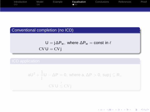
Conventional completion (no ICD)

U = j∆Pw , where ∆Pw = const in ℓ

CV U = CV j

ICD application

aU2 +1jU −∆P = 0, where a,∆P > 0, sup j ⊆ R+

CV U?

≤ CV j

Introduction Model Example Equalisation Conclusions References Proof

Conventional completion (no ICD)

U = j∆Pw , where ∆Pw = const in ℓ

CV U = CV j

ICD application

aU2 +1jU −∆P = 0, where a,∆P > 0, sup j ⊆ R+

CV U?

≤ CV j

Introduction Model Example Equalisation Conclusions References Proof

0

0.2

0.4

0.6

0.8

1

1.2

0 0.001 0.002 0.003 0.004 0.005 0.006 0.007

Channel ICD strength, bar/(Rm3/day)

2

CV

ratio

0

500

1000

1500

2000

2500

Well

flow

rate

, S

m3/d

ay

CoV ratio Well flow rate

0

0.2

0.4

0.6

0.8

1

1.2

0 2 4 6 8 10 12 14 16

Effective nozzle diameter per 40 ft joint, mm

CV

ratio

0

500

1000

1500

2000

2500

Well

flow

rate

, S

m3/d

ay

CoV ratio Well flow rate

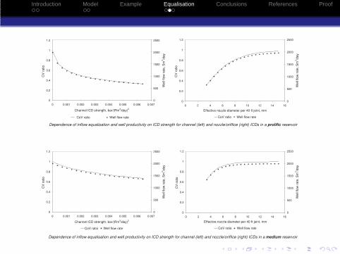
Dependence of inflow equalisation and well productivity on ICD strength for channel (left) and nozzle/oriffice (right) ICDs in a prolific reservoir

0

0.2

0.4

0.6

0.8

1

1.2

0 0.001 0.002 0.003 0.004 0.005 0.006 0.007

Channel ICD strength, bar/(Rm3/day)

2

CV

ratio

0

500

1000

1500

2000

2500

Well

flow

rate

, S

m3/d

ay

CoV ratio Well flow rate

0

0.2

0.4

0.6

0.8

1

1.2

0 2 4 6 8 10 12 14 16

Effective nozzle diameter per 40 ft joint, mm

CV

ratio

0

500

1000

1500

2000

2500

Well

flow

rate

, S

m3/d

ay

CoV ratio Well flow rate

Dependence of inflow equalisation and well productivity on ICD strength for channel (left) and nozzle/oriffice (right) ICDs in a medium reservoir

Introduction Model Example Equalisation Conclusions References Proof

Describe the distribution of j , η(j), rather than j(l)

qw =

∫ L

0U dℓ = L

∫ j2

j1

−1 +√

1 + 4a∆Pw j2

2ajη(j)dj

Calculation of CV ratio

〈U〉 = qw/L, 〈U2〉 =∫ j2

j1

(

−1 +√

1 + 4a∆Pw j2

2aj

)2

η(j) dj

CV U =

√

〈U2〉 − 〈U〉2

〈U〉 , CV j =

√

〈j2〉 − 〈j〉2

〈j〉

Results1 CV U ≤ CV j2 explicit analytical formulae for CV U/CV j when j has

uniform or triangular distribution (+ numerical estimation isalways possible)

Introduction Model Example Equalisation Conclusions References Proof

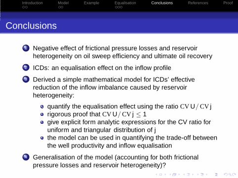
Conclusions

1 Negative effect of frictional pressure losses and reservoirheterogeneity on oil sweep efficiency and ultimate oil recovery

2 ICDs: an equalisation effect on the inflow profile

3 Derived a simple mathematical model for ICDs’ effectivereduction of the inflow imbalance caused by reservoirheterogeneity:

quantify the equalisation effect using the ratio CV U/CV jrigorous proof that CV U/CV j ≤ 1give explicit form analytic expressions for the CV ratio foruniform and triangular distribution of jthe model can be used in quantifying the trade-off betweenthe well productivity and inflow equalisation

4 Generalisation of the model (accounting for both frictionalpressure losses and reservoir heterogeneity)?

Introduction Model Example Equalisation Conclusions References Proof

Birchenko, V.M., Usnich, A.V., Davies, D.R. (2010) Impact offrictional pressure losses along the completion on wellperformance. J. Pet. Sci. Eng., doi: 10.1016/j.petrol.2010.05.019.

Birchenko, V.M., Muradov, K.M., Davies, D.R. (2010) Reductionof the Horizontal Well’s Heel-Toe Effect with Inflow ControlDevices. Under review in J. Pet. Sci. Eng.

Birchenko, V.M., Bejan, A.Iu., Usnich, A., Davies, D.R. (2010)Application of Inflow Control Devices to HeterogeneousReservoirs. Under review in J. Pet. Sci. Eng.

Birchenko, V.M., Al-Khelaiwi, F., Konopczynski, M., Davies, D.R.(2008) Advanced wells: how to make a choice between passiveand active inflow-control completions. In SPE Annual Tech.Conf.&Exhib., dx.doi.org/10.2118/115742-MS

More references in the proceedings paper.

Introduction Model Example Equalisation Conclusions References Proof

aU2 + U/j −∆P = 0, a,∆P > 0, supp j ⊆ R+

task: to prove that CV U/CV j ≤ 1

Y = U/√∆P, X = j

√∆P ⇒ aY 2 + Y/X − 1 = 0

CV Y = CV U, CV X = CV j, so will prove for X and Y

Define a cont. bijection x = y/(1 − ay2) from (0, a−1/2) to (0,∞)

F (a) =

∫

∞

0 x(y ; a)2 dh(y)(∫

∞

0 x(y ; a)dh(y))2 = 1 + (CV X)2 ; F (0) = 1 + (CV Y )2

Theorem

The function F satisfies the inequality F (0) ≤ F (a), where, except forthe case when a = 0, equality holds iff h is a point mass distribution.

Introduction Model Example Equalisation Conclusions References Proof

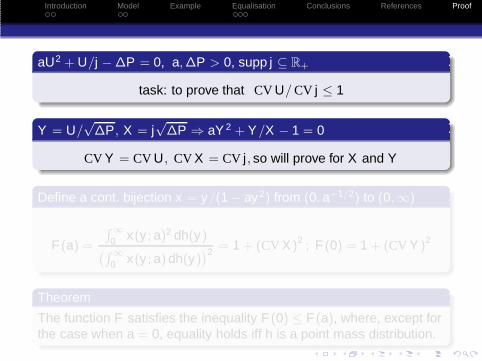
aU2 + U/j −∆P = 0, a,∆P > 0, supp j ⊆ R+

task: to prove that CV U/CV j ≤ 1

Y = U/√∆P, X = j

√∆P ⇒ aY 2 + Y/X − 1 = 0

CV Y = CV U, CV X = CV j, so will prove for X and Y

Define a cont. bijection x = y/(1 − ay2) from (0, a−1/2) to (0,∞)

F (a) =

∫

∞

0 x(y ; a)2 dh(y)(∫

∞

0 x(y ; a)dh(y))2 = 1 + (CV X)2 ; F (0) = 1 + (CV Y )2

Theorem

The function F satisfies the inequality F (0) ≤ F (a), where, except forthe case when a = 0, equality holds iff h is a point mass distribution.

Introduction Model Example Equalisation Conclusions References Proof

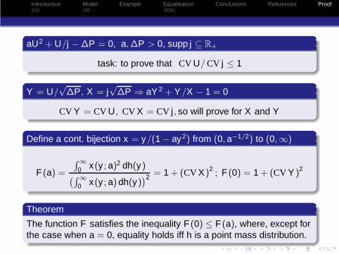
aU2 + U/j −∆P = 0, a,∆P > 0, supp j ⊆ R+

task: to prove that CV U/CV j ≤ 1

Y = U/√∆P, X = j

√∆P ⇒ aY 2 + Y/X − 1 = 0

CV Y = CV U, CV X = CV j, so will prove for X and Y

Define a cont. bijection x = y/(1 − ay2) from (0, a−1/2) to (0,∞)

F (a) =

∫

∞

0 x(y ; a)2 dh(y)(∫

∞

0 x(y ; a)dh(y))2 = 1 + (CV X)2 ; F (0) = 1 + (CV Y )2

Theorem

The function F satisfies the inequality F (0) ≤ F (a), where, except forthe case when a = 0, equality holds iff h is a point mass distribution.

Introduction Model Example Equalisation Conclusions References Proof

aU2 + U/j −∆P = 0, a,∆P > 0, supp j ⊆ R+

task: to prove that CV U/CV j ≤ 1

Y = U/√∆P, X = j

√∆P ⇒ aY 2 + Y/X − 1 = 0

CV Y = CV U, CV X = CV j, so will prove for X and Y

Define a cont. bijection x = y/(1 − ay2) from (0, a−1/2) to (0,∞)

F (a) =

∫

∞

0 x(y ; a)2 dh(y)(∫

∞

0 x(y ; a)dh(y))2 = 1 + (CV X)2 ; F (0) = 1 + (CV Y )2

Theorem

The function F satisfies the inequality F (0) ≤ F (a), where, except forthe case when a = 0, equality holds iff h is a point mass distribution.