Embed Size (px)
Citation preview
DENGUE RAPID DIAGNOSTICS VIA
SURFACE PLASMON RESONANCE BIOSENSOR
PEYMAN JAHANSHAHI
THESIS SUBMITTED IN FULFILMENT OF THE REQUIREMENTS
FOR THE DEGREE OF DOCTOR OF PHILOSOPHY
FACULTY OF ENGINEERING
UNIVERSITY OF MALAYA
KUALA LUMPUR
2015

UNIVERSITI MALAYA
ORIGINAL LITERARY WORK DECLARATION
Name of Candidate: Peyman Jahanshahi (I.C/Passport No:
Registration/Matric No: KHA100120
Name of Degree: DOCTOR OF PHILOSOPHY
Title of Project Paper/Research Report/Dissertation/Thesis (“this Work”):
Dengue Rapid Diagnostics via Surface Plasmon Resonance Biosensor
Field of Study: Photonic (Electronics and Automation)
I do solemnly and sincerely declare that:
(1) I am the sole author/writer of this Work;
(2) This Work is original;
(3) Any use of any work in which copyright exists was done by way of fair dealing and for permitted
purposes and any excerpt or extract from, or reference to or reproduction of any copyright work
has been disclosed expressly and sufficiently and the title of the Work and its authorship have
been acknowledged in this Work;
(4) I do not have any actual knowledge nor do I ought reasonably to know that the making of this
work constitutes an infringement of any copyright work;
(5) I hereby assign all and every rights in the copyright to this Work to the University of Malaya
(“UM”), who henceforth shall be owner of the copyright in this Work and that any reproduction
or use in any form or by any means whatsoever is prohibited without the written consent of UM
having been first had and obtained;
(6) I am fully aware that if in the course of making this Work I have infringed any copyright whether
intentionally or otherwise, I may be subject to legal action or any other action as may be
determined by UM.
Candidate’s Signature Date
Subscribed and solemnly declared before,
Witness’s Signature Date
Name:
Designation:

i
Dedication
I dedicate this curriculum to my wife,
MANIYA
, who did more than her share around the house as I sat at the computer.
Without her tireless love, support, and patience, I could not really enjoy
my scientific researches and complete my PhD.
ii
ABSTRACT
The aim of this thesis is to introduce an optical technique which can be utilized in
detection of dengue virus rapidly. This technique involves the application of analytical
and numerical electromagnetic simulations led by physical insight and theoretical
knowledge. As a part of this study, the most common permittivity function models are
compared and the best model is identified for the proposed biosensor structure. The
best model (Brendel-Bormann) is found to have an accuracy of ~94.4% with respect to
experimental data. On the other hand, Finite Element Method (FEM) is found to be a
valuable tool in the numerical solutions of the proposed biosensor structure throughout
this thesis.
Beside of simulation, the experiment is implemented through the Biacore device
which is based on the surface plasmon resonance (SPR) technique. According to the
experimental results, a serum volume of only 1 μl from a dengue patient (as a
minimized volume) is required to determine the ratio of each dengue serotype in
samples with 83-93% sensitivity and 100% specificity.
The Biacore device is considered in an effort to demonstrate a rapid diagnostic test
of dengue virus and the application of the intended technique in this detection. An
immobilization of dengue antigen is properly performed on the chip surface, and all
samples in four serotypes of dengue virus are examined through the chip. Beside the
determination of sensitivity and specificity of our detection method, an optimization of
sample volume is studied with different concentrations of samples. In addition, the
theoretical calculations are validated in comparison with experimental results.
According to the sample from each category of dengue serotypes 2 (low, mid, and
highly positive), the error ratio of ~5.35%, 6.54%, and 3.72% is obtained at the end.

iii
ABSTRAK
Tujuan tesis ini adalah untuk memperkenalkan teknik optik yang boleh digunakan
dalam mengesan virus denggi dengan cepat. Teknik ini melibatkan penggunaan
simulasi elektromagnet dan analisis berangka yang diterajui oleh wawasan fizikal dan
pengetahuan teori. Sebagai sebahagian daripada kajian ini, pelbagai model fungsi
ketelusan telah dibandingkan dan model yang terbaik untuk struktur biosensor
dikenalpasti. Model tersebut (Brendel-Bormann) menunjukkan ketepatan ~ 94.4%
dibandingkan dengan data eksperimen. Selain itu, didapati bahawa Kaedah Unsur
Terhingga (KUT) merupakan kaedah yang bernilai dalam penyelesaian berangka
struktur biosensor yang dicadangkan di seluruh tesis ini.
Selain daripada simulasi, eksperimen yang dilaksanakan melalui peralatan Biacore
berdasarkan teknik plasmon resonans permukaan. Menurut hasil kajian, hanya 1 μl
isipadu serum daripada pesakit denggi (jumlah minimum) diperlukan untuk
menentukan nisbah setiap serotype denggi dalam sampel dengan kepekaan 83-93% dan
penkhususan 100%.
Biacore telah dipertimbangkan dalam usaha kami untuk mendemonstrasikan ujian
diagnostik yang cepat untuk pengesanan virus denggi. Pernahanan antigen denggi
dilaksanakan di atas permukaan cip, dan semua sampel yang mengandungi empat
serotype virus denggi akan diteliti melalui cip. Selain menentukan kepekaan dan
pengkhususan bagi kaedah pengesanan kami, pengoptimuman isipadu sampel telah
dikaji dengan kepekatan yang berbeza sampel. Di samping itu, pengiraan teori telah
disahkan melalui perbandingan dengan keputusan eksperimen. Menurut sampel dari
setiap kategori serotype denggi 2 (rendah, pertengahan, dan sangat positif), nisbah ralat
sekitar ~ 5.35%, 6.54% dan 3.72% diperolehi.

iv
ACKNOWLEDGEMENTS
I would like to express my deep gratitude and appreciation to my supervisor,
Professor Dr. Faisal Rafiq Mahamd Adikan for his valuable guidance, support and
encouragement in both my academic work and life in general. I consider myself
fortunate to have had the chance to learn from such an excellent mentor.
I would like to thank the Integrated Lightwave Research Group previously known
as Photonics Research Group (especially Mostafa Ghomeishi, Saleh Seyedzadeh, Syed
Reza Sandoghchi) that helped me during my PhD. I would also like to thank the
University of Malaya High Impact Research Grant (MOHE-HIRG A000007-50001) at
UM for funding research and tuition fees.
I am very thankful to Professor Dr. Shamala Devi Sekaran from Faculty of
Medicine, UM, my research advisor, for all of her patience, and for her guidance in my
research work and other matters. I have very much enjoyed working and collaborating
with her and her group (especially Ms. Adeline Yeo Kin Lian) for assisting in
laboratorial works.
Finally, I cannot thank my family enough. Shamsi and Mohammad Jalil, my dear
parents / Zahra and Mohammad Hadi, my dear parents in-law, my dear brothers
(Mahdi, Kamran, and Pooriya), my dear sisters (Zahra, Nadiya and Shima), without
your continuous love and encouragement, I never could have accomplished my dreams.
I can only say that I love you with all my heart. Meanwhile, welcome to Saniya, my
daughter, that has been born recently. My life would be incomplete without the blessing
of your continuous patience, support, and love.
Thanks you, Almighty God, for giving me all these wonderful people in my life.

v
LIST OF CONTENTS
ABSTRACT....................................................................................................... ii
ABSTRAK ........................................................................................................ iii
ACKNOWLEDGEMENTS .............................................................................. iv
LIST OF CONTENTS ....................................................................................... v
LIST OF TABLES .......................................................................................... viii
LIST OF FIGURES .......................................................................................... ix
LIST OF SYMBOLS ....................................................................................... xv
1 CHAPTER I: INTRODUCTION .................................................................. 1
1.1 Introduction ......................................................................................... 1
1.2 Research background ........................................................................... 4
1.2.1 Laboratory Diagnosis .......................................................................... 6
1.3 Statement of problem......................................................................... 14
1.4 Objectives .......................................................................................... 15
1.5 Overview of the study........................................................................ 16
2 CHAPTER II: THEORY AND BACKGROUND OF SURFACE
PLASMONS ................................................................................................. 17
2.1 Introduction ....................................................................................... 17
2.2 Theoretical background of electromagnetic ...................................... 18
2.2.1 Maxwell’s equations in differential form .......................................... 19
2.2.2 Energy Conservation and the Poynting vector .................................. 19
2.2.3 Wave equations .................................................................................. 21
2.3 Introduction to optics and surface plasmons ..................................... 23
2.3.1 History of Surface Plasmon Resonance ............................................. 23
2.3.2 Surface plasmon concept ................................................................... 25
2.3.3 Surface plasmon excitation ................................................................ 26
2.3.3.1 Excitation by Electrons ................................................................ 26
2.3.3.2 Excitation by Photons .................................................................. 27
2.3.4 Otto and Kretschmann configurations ............................................... 28
2.3.5 Surface plasmon polaritons ............................................................... 29
2.3.6 Surface Plasmon Resonance .............................................................. 29
2.4 Planar Surface Plasmons ................................................................... 33
2.4.1 Surface plasmons in three-layer configuration .................................. 38
2.4.2 Theoretical background of SPs in DMD structure ............................ 39
2.4.3 Symmetric and anti-symmetric modes of SPs in DMD structure ..... 43
2.5 Analysis methods applied in this study ............................................. 48
2.5.1 Analytical Analysis............................................................................ 49
2.5.2 Numerical Analysis ........................................................................... 50

vi
2.6 The application of surface plasmons in sensing ................................ 51
3 CHAPTER III: METHOD AND PROCEDURE .......................................... 54
3.1 Overview ........................................................................................... 54
3.2 Optical properties of metallic films ................................................... 54
3.2.1 Common models for optical properties of thin metallic films ........... 54
3.2.1.1 Drude model ................................................................................ 55
3.2.1.2 Drude-Lorentz model .................................................................. 56
3.2.1.3 Brendel-Bormann model ............................................................. 56
3.2.1.4 Multi oscillator model ................................................................. 57
3.2.2 Reference data of optical properties of proposed thin films .............. 58
3.3 Method of analytical and numerical analysis on SPR configuration. 61
3.3.1 Analytical analysis of SPR configuration .......................................... 61
3.3.1.1 Refection and transmission of polarized light by stratified planar
structures ............................................................................................ 61
3.3.2 Numerical analysis of SPR configuration ......................................... 65
3.4 Implementation of the proposed SPR structure ................................. 67
3.4.1 Use of gold as the metal layer ........................................................... 67
3.4.2 Surface plasmons on dielectric-metal-dielectric waveguides ............ 67
3.5 Molecular interactions in modeling the SPR biosensors ................... 69
3.6 Method of experiment ....................................................................... 70
3.6.1 A simple experiment .......................................................................... 70
3.6.2 Measurement of the SPR angle shift ................................................. 71
3.6.3 Basics of Biacore set-up and chip construction ................................. 72
3.6.4 Buffer Solutions for measuring the analysis cycle ............................ 74
3.6.4.1 Baseline buffer ............................................................................. 74
3.6.4.2 Required solutions during an assay ............................................. 75
3.6.4.3 Regeneration solution .................................................................. 75
3.6.5 From surface plasmon to SPR signal ................................................. 75
3.6.6 Cycle of virus detection using scanning SPR imaging ...................... 77
3.6.7 Measurement of the analysis cycle: scanning SPR microarray imaging
of autoimmune diseases ..................................................................... 79
3.6.7.1 Introduction ................................................................................. 79
3.6.7.2 Ligand immobilization ................................................................ 80
3.6.7.3 The Analysis cycle for measuring biomolecular interactions ..... 82
3.6.8 The whole process of an assay .......................................................... 83
3.6.9 Sample Collection.............................................................................. 86
3.6.10 Investigation of sample concentration - calibration curve ................. 86
3.6.11 Clinical samples ................................................................................. 88
4 CHAPTER IV: RESULTS AND DISCUSSIONS ....................................... 90

vii
4.1 Introduction ....................................................................................... 90
4.2 Mode and propagation analysis of general SPR configuration ......... 90
4.2.1 Mode analysis of symmetric SPPs..................................................... 90
4.2.2 Propagation analysis of symmetric SPPs........................................... 91
4.3 Numerical analysis for surface binding affinity ................................ 93
4.4 Investigation of optical properties models on SPR structure ............ 95
4.4.1 Comparison between common optical properties models for metallic
thin films ............................................................................................ 95
4.4.2 Analytical analysis of the models on SPR structure .......................... 99
4.4.3 Numerical analysis of the models on SPR structure ........................ 101
4.5 Sensor signal of immobilization process ......................................... 103
4.6 Microscopic information of chip sensor .......................................... 104
4.7 Determination of sample concentration ........................................... 107
4.8 Examination of samples................................................................... 111
4.9 Validating simulation based on experimental results ...................... 117
5 CHAPTER V: CONCLUSION AND FUTURE WORK ........................... 120
APPENDIX A: Derivation dispersion relation; SP’s on planar surface ........ 122
APPENDIX B: Investigation of chip surface ................................................ 124
I. Atomic force microscopy image ...................................................... 124
II. Scanning electron microscope image .............................................. 125
APPENDIX C: List of Publications, patent and innovation .......................... 127
REFERENCES .............................................................................................. 130

viii
LIST OF TABLES
Table 1.1 Laboratory Methods (ELISAs) ................................................................... 12
Table 1.2 Commercial rapid diagnostic tests for detection of dengue virus ............... 13
Table 3.1 Refractive index (nr) and absorption coefficient (ni) of gold (Schulz &
Tangherlini, 1954; Schulz, 1954) ................................................................................ 59
Table 3.2 Refractive index (nr) and absorption coefficient (ni) of titanium (Schulz &
Tangherlini, 1954; Schulz, 1954) ................................................................................ 60
Table 4.1 Comparative data base of ELISA and proposed SPR biosensor in low, mid
and high positive patient samples of dengue virus.................................................... 114
Table 4.2 The negative controls and the number of the serum samples were examined
for the specificity evaluation in this study. ............................................................... 116
Table 4.3 The SPR variations of three categorized serums analytically and
experimentally, and their mathematical error ........................................................... 119

ix
LIST OF FIGURES
Figure 1.1 Global evidence consensus, risk and burden of dengue in 2010. Courtesy
(Bhatt et al., 2013) ......................................................................................................... 3
Figure 1.2 Number of dengue cases by week, Department of Health, Malaysia .......... 4
Figure 1.3 Characterization of dengue fever ................................................................. 5
Figure 1.4 Flowchart of dengue IgM capture enzyme linked imunosorbent assay
method ........................................................................................................................... 9
Figure 1.5 Major diagnostic markers for dengue infection (Peeling et al., 2010) ...... 10
Figure 1.6 Test procedure of the rapid dengue fever diagnosis, adapted from Standard
Diagnostics (SD) Inc. database ................................................................................... 11
Figure 2.1 A simple schematic of a surface plasmon.................................................. 25
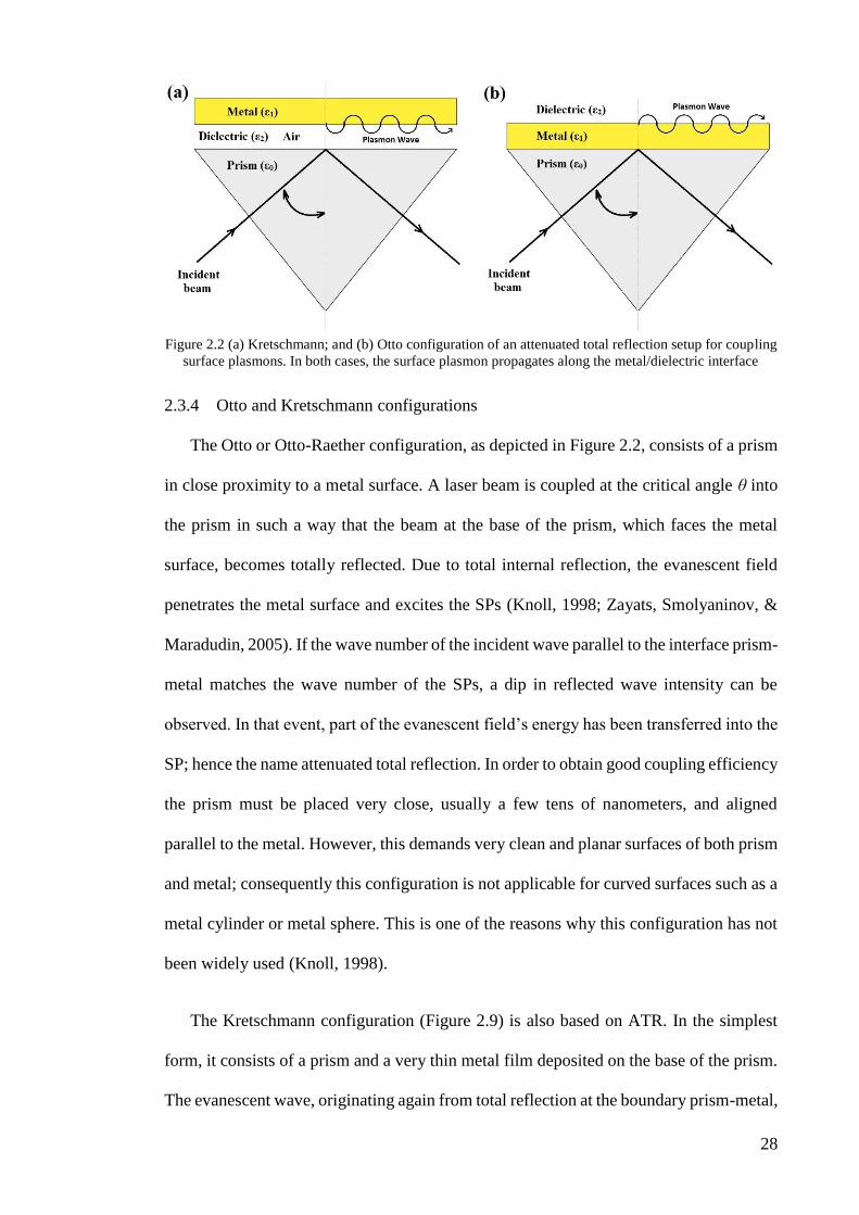
Figure 2.2 (a) Kretschmann; and (b) Otto configuration of an attenuated total reflection
setup for coupling surface plasmons. In both cases, the surface plasmon propagates
along the metal/dielectric interface ............................................................................. 28
Figure 2.3 The surface plasmon mode (wave) is excited at the interface between a metal
film and dielectric medium using a light wave ........................................................... 31
Figure 2.4 Concept of surface plasmon resonance sensors ......................................... 31
Figure 2.5 Intensity of light wave interacting with a surface plasmon as a function of
angle of incidence ....................................................................................................... 32
Figure 2.6 (a) Direct and (b) Indirect SPR sensors: measurand and sensor output .... 32
Figure 2.7 3D model of surface plasmon propagating along a flat metal surface in the
x-direction; A snapshot of the Hy distribution (TM mode) is schematically shown. The
relative permittivity 휀𝑑 is for the dielectric material and e is for the metal. The
evanescent waves in the y-direction are indicated by the dash-dotted line. ................ 35
Figure 2.8 Propagation length for SPs on a planar surface for gold, silver and aluminum
(Vogel, 2009) .............................................................................................................. 37
x
Figure 2.9 Dispersion relation of SPs on a flat Ag surface, with the permittivity of Ag
modeled by Drude-Lorentz Model; λ𝑝 is the corresponding plasmon wavelength and
휀𝑑 = 1 is the permittivity of the adjacent dielectric material. See text for curve
descriptions. ................................................................................................................ 38
Figure 2.10 Three-layer dielectric-metal-dielectric waveguide structure ................... 40
Figure 2.11 3D image of SPs propagating along a metal film (DMD structure) with (a)
anti-symmetric and (b) symmetric magnetic field distribution with respect to the middle
plane ............................................................................................................................ 42
Figure 2.12 Dispersion relation qx(h), where h is the film thickness of a DMD plasmon
waveguide for symmetric and anti-symmetric magnetic field Hy. Effective index and
modal attenuation of surface plasmons propagating along thin gold film (εm= -25 +
1.44i) slotted in between two dielectrics (nd1=1.32 and nd2= 1.35) as a function of gold
film thickness; wavelength is 800nm .......................................................................... 44
Figure 2.13 Field profile of symmetric (left side plots) and anti-symmetric (right side
plots) surface plasmon on thin gold film (εm= – 25 + 1.44i) between two identical
dielectrics (nd1= nd2= 1.32); gold film thickness is 20nm and wavelength is 800nm. 46
Figure 3.1 N-layer model for SPR measurement. ....................................................... 62
Figure 3.2 SPR curve (red line) with the BK7 galss prism|gold|air, and SPR curves
(blue lines) with the BK7 prism|gold|binding medium|air configurations. ................. 64
Figure 3.3 The scheme of SPR structure for numerical modeling .............................. 66
Figure 3.4 Configuration of the modeled structure in this study ................................ 68
Figure 3.5 The SPR structure, dielectric II-gold-dielectric I waveguide structure ..... 68
Figure 3.6 Schematic fundamental set-up of SPR excitation. A biosensor with a gold
film coating is placed on a prism. The polarized light propagates from the light source
on the sensor surface. .................................................................................................. 71

xi
Figure 3.7 The sensorgram of angle (can be termed as resonance unit) versus time. At
first, no change occurs in the sensorgram. In state A, a baseline is measured with the
dip at SPR angle. After injecting the sample, which adsorbs on the sensor surface,
producing a change in refractive index and consequently a SPR angle change to the
state B. In real time, the adsorption–desorption procedure can be followed and then the
amount of adsorbed specific biomolecular can be determined. .................................. 72
Figure 3.8 The detection approach of Biacore SPR setup. The SPR reaction is correlated
to refractive index changes at the surface of biosensor, caused by changing
concentration of the binding medium when the antibodies as a target bind to the
immobilized antigens as a probe ................................................................................. 74
Figure 3.9 Biacore 3000 system with controller unit .................................................. 76
Figure 3.10 Rotated presentation of the SPR dip (left section) that forms directly the
pointer of the sensorgram (right section). The angle shift of the SPR dip is determined
(left, A to B), followed by plotting the angle of the SPR minimum in the sensorgram
vs. time (right). Here the SPR dip minimum of the initial curve (A) shifts with time
towards a larger angle (B). .......................................................................................... 76
Figure 3.11 The liquid delivery system with two pumps and an autosampler transports
liquid to the connector block where samples and buffers are injected to the IFC. The
scheme adapted from ref. (GE Healthcare, 2008). ...................................................... 79
Figure 3.12 Schematic of the dengue virus diagnosis process-ligand immobilization
part............................................................................................................................... 81
Figure 3.13 Immobilization sensorgram of the dengue antigen on sensor surface: (a)
Baseline; (b) using EDC/NHS for surface activation; (c) baseline after activation; (d)
attraction and covalent coupling of the ligand; (e) buffer washes away loosely
associated ligand; (f) deactivation and further washing away loosely associated ligand;
(g) the final response of immobilization. .................................................................... 82

xii
Figure 3.14 Schematic of the dengue virus diagnosis process-virus detection part .... 84
Figure 3.15 A sensorgram which is shown the all phases of an analysis cycle .......... 85
Figure 3.16 Schematic of data management of each assay ......................................... 86
Figure 3.17 Flow chart of the test concentration and regeneration of biosensor. ....... 87
Figure 3.18 The samples from four different serotypes of dengue virus which have been
categorized to the three groups ................................................................................... 88
Figure 3.19 Some samples with tick-borne encephalitis (TBE) and hepatitis C (HC)
antibodies .................................................................................................................... 89
Figure 4.1 Mode analysis of the proposed structure. (a) Mesh structure near and within
the metal strip. (b) Total energy density time average. (c-h) fields distributions: Hx, Hy,
Hz, Ex, Ey, and Ez respectively .................................................................................... 91
Figure 4.2 Three dimensional simulation of the proposed model. (a) Mesh structure.
(b) Energy density time average distribution of the light. (c-h) Field distributions. .. 93
Figure 4.3 The presence of magnetic field in z component by numerical modeling of
biosensor structure, (I) is with sample’s refractive index of 1.33 and (II) is with
sample’s refractive index of 1.34 ................................................................................ 94
Figure 4.4 Numerical analysis of biosensor structure with refractive index 1.33 to 1.34
..................................................................................................................................... 95
Figure 4.5 Real part of permittivity (F/m) against wavelength (nm) of experimental
data, and Multi Oscillator, Drude-Lorentz, Brendel-Bormann, Drude models .......... 96
Figure 4.6 Error value at real permittivity (%) against wavelength (nm) ................... 97
Figure 4.7 Imaginary part of permittivity (F/m) against wavelength (nm) of
Experimental Data, and Multi Oscillator, Drude-Lorentz, Brendel-Bormann, Drude
models ......................................................................................................................... 98
Figure 4.8 Error value at imaginary permittivity against wavelength ........................ 98
Figure 4.9 Reflectance against incident angle of 30 to 70 degree, at 600nm ........... 100

xiii
Figure 4.10 SPR angle (degree) against wavelength of 560nm to 760nm ................ 101
Figure 4.11 Error value at SPR angle for wavelength of 560nm to 760nm .............. 101
Figure 4.12 Comparison between using experimental data and Brendel-Bormann model
at energy density time average distribution of the light ............................................ 103
Figure 4.13 Immobilization sensorgram of four serotypes of dengue antigen on sensor
surface ....................................................................................................................... 104
Figure 4.14 Imaging of the immobilization process on the gold surface using SEM 104
Figure 4.15 Imaging of the immobilization process on the gold surface using SEM
machine- .................................................................................................................... 105
Figure 4.16 Two dimensional AFM image dengue antigen-dextran conjugate onto
surface ....................................................................................................................... 106
Figure 4.17 Three dimensional AFM image dengue antigen-dextran conjugate onto
surface ....................................................................................................................... 106
Figure 4.18 Sensorgrams illustrate the evolution of resonance units (RU) versus time
during association and dissociation measurements along with biosensor regeneration
performed in the Biacore instrument. The inset schematics represent dengue antibodies
(Y shapes) versus dengue antigens (immobilized circles on surface) ....................... 108
Figure 4.19 (Blue) The stacked column graph represents the quantity of Ag-Ab bound
on the sensor surface, which is directly related to the amount of sensor sensitivity; Red
represents chip surface cleaning related to the quality of sensor regeneration ......... 111
Figure 4.20 The binding response curve termed by sensorgram, (a) the binding process
and (b) the regeneration of biosensor surface ........................................................... 112
Figure 4.21 SPR angle variation via patient's serum- Dengue virus diagnosis graph
................................................................................................................................... 113
Figure 4.22 Patients’ serum via SPR angle variation, and their refractive index changes
................................................................................................................................... 117

xiv
Figure 4.23 The shift of SPR angle which is indicated by reflectivity versus angle of
incidence obtained from clinical analysis ................................................................. 119

xv
LIST OF SYMBOLS
Ab Antibody
ADE Antibody-Dependent Enhancement
AFM Atomic Force Microscopy
Ag Antigen
ATR Attenuated Total Reflection
ATR Attenuated Total Reflection
B Magnetic-Flux Density
B-B Brendel Bormann Model
D Drude Model
D Flux Density
DF Dengue Fever
DHF Dengue Hemorrhagic Fever
D-L Drude-Lorentz Model
DMD Dielectric-Metal-Dielectric
DSS Dengue Shock Syndrome
E Electric Field
EELS Electron Energy Loss Spectrometry
EIM Effective Index Method
ELISA Enzyme-Linked Immune-Sorbent Assay
EM Electromagnetic
FDTD Finite-Difference Time-Domain
FEM Finite Element Method
H Magnetic Field
HC Hepatitis C
HCT Hematocrit
xvi
IgG Immunoglobulin G
IgM Immunoglobulin M
MDM Metal- Dielectric-Metal
M-O Multi Oscillator Model
NS1 Non Structural protein 1
PCR Polymerase Chain Reaction
POC Point of Care
R Reflectance
RDTs Rapid Diagnostic Tests
RU Resonance Units
S Poynting vector
SEM Scanning Electron Microscopy
SP Surface Plasmon
SPP Surface Plasmon Polariton
SPR Surface Plasmon Resonance
TBE Tick-Borne Encephalitis
TE Transverse Electric
TEM Transmission Electron Microscope
TM Transverse Magnetic
WHO World Health Organization
ε Dielectric Constant
µ Magnetic Permeability

1
1 CHAPTER I: INTRODUCTION
1.1 Introduction
Infectious diseases or communicable diseases are caused by the presence of
pathogenic microorganisms, such as bacteria, viruses, fungi or parasites. The diseases can
be spread, directly or indirectly, from one person to another (Cheesbrough, 2006). The
disease transmission may occur through one or more of diverse pathways including
physical contact with infected individuals. These infecting agents may also be transmitted
through liquids, food, body fluids, contaminated objects, airborne inhalation, or through
vector-borne spread. The dominant cases of infectious diseases include lower respiratory
infections, HIV/AIDS, Tetanus and tropical diseases such as dengue fever, malaria, and
tuberculosis(Lim, 2009; Mathers, Fat, & Boerma, 2008).
Dengue and dengue hemorrhagic fever (DHF) are caused by one of four closely
related, but antigenically distinct, virus serotypes (DEN-1, DEN-2, DEN-3, and DEN-4),
of the genus Flavivirus (Gubler & Clark, 1995). Infection with one of these serotypes
does not cross-protect, so persons living in a dengue-endemic area can have up to four
dengue infections during their lifetimes. Dengue is an urban disease of the tropics and
subtropics, and its causative agent can be maintained in a cycle that involves humans and
its vectors (Aedes aegypti and aedes albopictus). Dengue has been chosen as the test bed
for this project as it is one of the local and emerging diseases in the tropical and
subtropical regions with high fatality rate (Dutra, de Paula, de Oliveira, de Oliveira, &
De Paula, 2009). Infection with a dengue virus can generate a spectrum of clinical
sickness from non-specific viral syndromes to critical and fatal hemorrhagic illness.
Significant risk factors for DHF consist of the strain and the virus serotype involved,
immune status, genetic predisposition, and age of the patient (Bhatt et al., 2013).

2
There is an annual report that estimated hundred million cases of the dengue fever
(DF) and 250,000 - 500,000 cases of the DHF with the average case fatality rate being
5% in the world (Guzman et al., 2010; Honório et al., 2009). The half of world’s
population lives in zones with high risk of dengue infection and these zones are common
destinations as well. The world’s population is estimated to be 8.3 billion on 2025 with
the increase happening in urban settlements. This has caused an unplanned and
uncontrolled urbanization of the developing countries particularly in tropical areas (D. S.
Shamala, 2005). The first case of occurred dengue epidemic was reported in 1779-1780
in Asia, Africa, and North America (Gubler & Clark, 1995).
In the latest report 2013, national and subnational evidence consensus on complete
absence (green) through to complete presence (red) of dengue (Figure 1.1 (a)), probability
of dengue occurrence at 5 km × 5 km spatial resolution of the mean predicted map from
336 boosted regression tree models (Figure 1.1 (b) and (c)) cartogram of the annual
number of infections for all ages as a proportion of national or subnational (China)
geographical area (Figure 1.1 (c)) are presented (Bhatt et al., 2013).
Malaysia is one of the tropical countries with notably high mortality and morbidity
cases of tropical diseases especially of dengue fever. The Dengue virus is a typical
tropical disease because the mosquitos that carry the virus require a warm and hot climate
(Special Programme for Research, Training in Tropical Diseases, 2009).

3
Figure 1.1 Global evidence consensus, risk and burden of dengue in 2010. Courtesy (Bhatt et al., 2013)
In 1902, the first case of dengue fever in Malaysia was reported through the dengue
outbreak in Penang by Skae. More reports were published on dengue outbreaks in
numerous states of Peninsular Malaysia mostly in large cities and ports in 1904, 1932 and

4
1933 subsequently (D. S. Shamala, 2005). For the first time, the dengue virus was isolated
by Smithburn in 1950. In 1953, the laboratory confirmation was first performed by the
Institute of Medical Research in Malaysia. Since that time, the pockets of outbreaks began
to appear in urban zones of Peninsular Malaysia, and the dengue fever is become a
notifiable disease in this tropical region. From then on increasing the numbers of dengue
patient were recorded in Malaysia (D. S. Shamala, 2005; D. Shamala, 2008).
Figure 1.2 Number of dengue cases by week, Department of Health, Malaysia
According to the latest report as of 20th December 2014 (reported by WHO), the
number of dengue cases in Malaysia is still higher than for the same period in 2013. There
has been an increase of 16.4% in the number of reported new cases compared with the
previous week (Figure 1.2).
1.2 Research background
Dengue fever and its more serious forms, dengue hemorrhagic fever and dengue
shock syndrome (DSS), are becoming important public health problems and were
formally included within the disease portfolio of the of World Health Organization
(WHO) special program for research and training in tropical disease by the Joint
Coordination Board in June 1999. The global prevalence of dengue has grown
dramatically in recent decades (Lee, 2008; Shu & Huang, 2004). According to the WHO,
5
around 3.6 billion people are now at risk from Dengue (Dussart et al., 2008; Guzman et
al., 2010; Organization & others, 2011; Osman, Fong, & Devi, 2007). Currently, the
disease is endemic in over 100 tropical and sub-tropical countries and it is estimated that
there are 390 million cases of Dengue infections worldwide every year (Bhatt et al., 2013;
Murray, Quam, & Wilder-Smith, 2013).
Dengue infection may be without symptoms or cause to a series of clinical
presentations even in death level. Its incubation period is 4 to 7 days in the range of 3 to
14 days. The clinical symptoms consist of an itchy rash, nausea, sudden onset of fever,
muscle and joint pain, depression, frontal headache, weakness, vomiting and retro-orbital
pain (Figure 1.3). The feverish painful period of dengue fever continues 5 to 7 days, and
may leave the tired feeling in dengue patients for more than expected days (Rigau-Pérez
et al., 1998; D. S. Shamala, 2005).
Figure 1.3 Characterization of dengue fever
DSS is the most serious form and is specified as DHF with symptoms of frank shock,
circulatory failure, hypotension, and narrowing pulse pressure. The expansion of these
kinds of symptoms or any sign of hypotension presents the indications for hospital
admission and then managing patient. Prognosis is related to the prevention or rapid
diagnosis, and after that treatment of shock. According to the experience of specialists,
the case fatality rate (CFR) can be as low as 0.2% in hospitals. Once shock has appointed

6
in the CFR, it may be as high as 12 to 44%. There have been some uncommon but well
described indications of dengue fever like dengue infection with severe haemorrhage,
liver injuries, encephalopathy, and cardiomyopathy that the risk of death is high.
Neurological indications such as convulsions, altered consciousness, and coma have been
also reported (Ranjit & Kissoon, 2011; Rigau-Pérez et al., 1998; D. S. Shamala, 2005).
The risk of DHF is higher when two or more viruses circulate at the same time. In
addition, the presence of dengue antibodies obtained either actively by previous infection
or passive by maternal antibodies in the milk or in the uterus are some of the contributing
factors. Therefore antibodies actually enhance viral infectivity in the non-neutralising
concentrations. This assumption is termed by antibody-dependent enhancement (ADE) is
the process in which the virus is mixture with specific antibodies to enhance its absorption
by mononuclear cells (the primary part for replicating virus). The replication of the virus
in these cells affects the release of vasoactive mediators that increases vascular
permeability and the hemorrhagic symptoms that can observe in DHF (Rigau-Pérez et al.,
1998). But this assumption is inconsistent as there is a small but unanimous percentage
of the DHF/DSS cases which are caused by the primary infections. There is no pre-
existing antibodies in these persons (D. S. Shamala, 2005).
1.2.1 Laboratory Diagnosis
Conventional methods as laboratory diagnosis and rapid diagnostic tests (RDTs) are
two significant categories for use in biomedical diagnostics. For the laboratory diagnosis
of dengue fever as a common way, when a patient is suspected with dengue, he/she has
to go to a hospital to get a battery of diagnostic tests which require expensive equipment
and expertise which is not necessarily available if the patient came from a rural
background. The test is usually done in batches and results typically take time around 3-
7
7 days. By that time, the patient might be in critical stage and may not be referred to the
hospital on time for optimum clinical management (Rigau-Pérez et al., 1998).
Dengue virus belongs to the family Flaviviridae, a family which consists of around
70 viruses that have a cross-react in the serological tests. Since those share the blood
group antigens, therefore there is a complicating diagnosis. The laboratory diagnosis is
dependent upon the virus isolation and the serologic tests. There is a circulating virus that
remains detectable in blood during a feverish period after which those are recognized and
then cleared rapidly with appearance of the specific antibody. The virus isolation is
performed using the mosquito cell line. After a few days incubation, the virus is detected
through an indirect fluorescent antibody test.
The serological diagnosis is dependent on the presence of the immunoglobulin M
(IgM) antibodies or an increase in the immunoglobulin G (IgG) antibodies in paired acute
and convalescent phase serum. Over 90% of patients have the IgM positive test by the 4th
day of sickness, but the IgM antibodies may be due to infection up to three months earlier.
The commercial biochemical kits for the measurement of antibodies contain the enzyme-
linked immune-sorbent assay (ELISA), dipstick, and rapid dot blot tests. There is not
necessary to require a specialized training for these tests, but their specificity and
sensitivity are not steady state, reliable, and mainly low. It is true that the specificities of
ELISA kits are almost 100%, but the sensitivities of these kits have been examined around
87–90%. In rapid diagnostic tests, the sensitivity is in the range of 75–80% while these
types of rapid tests have not significantly enough specificity to distinguish between cross-
reactivity in the serological tests (Wang & Sekaran, 2010).
The polymerase chain reaction (PCR) is a biochemical method in the molecular
biology used to replicate a single or a few pieces of the DNA upon several orders of
magnitude, producing the millions of identical copies of a unique DNA sequence. The

8
multiplex PCR which was developed at the University of Malaya Medical Centre, is
capable to detect the serotype of virus detection in an approximate time 3-4 hours with
~75% sensitivity. The real time multiplex test that is capable to detect the dengue serotype
and viral RNA quantity, can examine a patient sample within an approximate time of two
and half hours with sensitivity ~89%. Both tests can be developed to amplify a virus
RNA from the onset of the infection. The detection of NS1 protein has been presented by
few researchers that show an applicable assay within acute phase of an illness (D. S.
Shamala, 2005; Yager, Domingo, & Gerdes, 2008).
It is true that the use of PCR technique may make to detect in the short time with
significantly high sensitivity and specificity, but this technique cannot be applicable when
the virus is completely gone in patient blood. In this phase, detection is performed through
the anti-virus existing in the blood (Fatemeh et al., 2014; Ramirez et al., 2009; Sabatino,
Botto, Borghini, Turchi, & Andreassi, 2013; D. S. Shamala, 2005).
Currently few commercial kits are available for dengue detection, but all kits need to
be extensively validated to assess their role in routine dengue diagnosis (Hunsperger et
al., 2009). Hence with these assays available it appears that two or more assays have to
be done to ensure maximal detection of the disease which yearly results in sporadic
outbreaks. The number of cases in the country warrants the need for diagnosis not only
to be precise but also sensitive and be able to diagnose with just one sample. The cost of
individual assays as well as confirmation makes this disease an expensive one to
diagnose. There are a lot of techniques to detect either virus specific proteins or
antibodies, but those can detect intact viral particles rarely. The ELISA is one of the most
conventional techniques for detection of viruses and viral specific antigens (Nunes et al.,
2011; He et al., 2009; Young, Hilditch, Bletchly, & Halloran, 2000).

9
The ELISA technique (Duzgun, Schuntner, Wright, Leatch, & Waltisbuhl, 1988),
however, has some limitations, such as cannot distinguish the source of antigen directly,
and needs laboratory sequential steps to detect the viruses. These steps consist of injection
some solutions to samples, incubation times, and keeping samples to specific temperature
(Figure 1.4).
Figure 1.4 Flowchart of dengue IgM capture enzyme linked imunosorbent assay method
The manifestation of the dengue disease is complex; however, the treatment of the
disease can be simple, inexpensive and effective as long as correct and early detection is
performed. This can only be achieved if understanding of the clinical problems and the
phases of the disease is known especially when patients are first seen and evaluated
through triage. Triage is a process of screening suspected patients to identify the severity

10
of the dengue patient’s condition. For proper management of the disease, a full blood
count should be done at the first visit or triage. While a hematocrit (HCT) test establishes
the patient’s own baseline, a decreasing white blood cell count indicates high likelihood
of dengue. A rapid decrease in platelet with rising HCT suggests progress to the critical
phase of the disease.
Up to now, the ELISA technique has been used to quantify various concentrations of
antibody or antigen in biological sample. It is commonly used for dengue detection of
Non Structural protein 1 (NS1) (Kumarasamy, Chua, et al., 2007; Kumarasamy, Wahab,
et al., 2007), Immunoglobulin M (IgM) (Guzman et al., 2010; Nunes et al., 2011; Shu et
al., 2003), and Immunoglobulin G (IgG) (Wang & Sekaran, 2010).
Figure 1.5 Major diagnostic markers for dengue infection (Peeling et al., 2010)
In serological approach, creation of immunoglobulins (IgM, IgG, and IgA) is the
reaction of the immune system to infections. These immunoglobulins are particular to
virus (E) protein. Depending on the patient’s condition, namely, whether or not they have
a primary or secondary infection, the sharpness of the response changes (Schilling,
Ludolfs, Van An, & Schmitz, 2004). Usually, the IgM response in the primary infection
11
has higher titre in comparison to the secondary one as shown in Figure 1.5 (Guzman et
al., 2010; Peeling et al., 2010).
However, common ELISA method is a slow process due to the required incubation
times (from a few hours to 2 days), and does not provide enough sensitive method in non-
laboratory settings typical of the point of care (POC) (Yager et al., 2008). The automated
ELISA system requires high-level expertise, expensive bulky equipment not available at
many hospitals and consumes considerable amount of chemicals (Guzman et al., 2010;
Hunsperger et al., 2009; Peeling et al., 2010).
Table 1.1 shows several commercial kits for the detection of antibody for
identification of dengue virus (Hunsperger et al., 2009). For screening purposes,
immunoassay method (ELISA), dipstick and also rapid test using the immune-
chromatographic dot blot are the most popular. The sensitivity of ELISA kits is around
96-98% with almost 100% specificity. For rapid diagnostic tests (Table 1.2), sensitivities
were obtained in range of 65-84% (C T Sang, Hoon, Cuzzubbo, & Devine, 1998).
Figure 1.6 Test procedure of the rapid dengue fever diagnosis, adapted from Standard Diagnostics (SD)
Inc. database

12
Table 1.1 Laboratory Methods (ELISAs)
Company,
location
Panbio
Diagnostics,
Windsor,
Queensland,
Australia
Bio-rad,
HERCULES,
CA, USA
Omega
Diagnostics,
Alva, UK
Focus
Diagnostics,
Cypress, CA,
USA
Standard
Diagnostics,
Kyonggi-do,
South Koreai
Existing Tests IgM and IgG NS1, IgM and
IgG IgM and IgG IgM and IgG
NS1, IgM and
IgG
Technique Biochemical Biochemical Biochemical Biochemical Biochemical
Format 12 strips of 8
wells
12 strips of 8
wells
12 strips of 8
wells
12 strips of 8
wells
12 strips of 8
wells
No.
tests/package 96 96 96 96 96
Antigen Recombinant
DENV 1–4
Purified
DENV 2 DENV 1–4 DENV 1–4 DENV 1–4
Sample
volume, µL 10 10 20 10 10
Total
incubation
time
130 min at
37°C
120 min at
37°C
110 min at
37°C
240 min at
room
temperature
130 min at
37°C
Storage
conditions, °C 2–30 2–8 2–8 2–8 2–8
Specimen type Only Serum Only Serum Only Serum Only Serum Only Serum
Sensitivity (%) 99.0 70-84 62.3 98.6
98.2 for NS1
96.4 for IgM
98.1 for IgG
Specificity (%) 79.9-86.6 94-100 97.8 79.9-86.6
100 for NS1
96.7 for IgM
98.9 for IgG
Rapid immune chromatography method also known as rapid diagnostic test (RDT) is
another option for detection of dengue infection (Initiative & others, 2005; Chew Theng
Sang, Hoon, Cuzzubbo, & Devine, 1998; Vaughn et al., 1998). The method is
characterized by its ease of use and rapid detection rate, requiring only a drop of
serum/plasma for diagnosis as shown in Figure 1.6.
i SD kits currently used in UM Medical Centre.

13
Table 1.2 Commercial rapid diagnostic tests for detection of dengue virus
Company,
location
Panbio
Diagnostics,
Australia
Bio-rad,
HERCULES,
CA, USA
Pentax,
Tokyo, Japan
Zephyr
Biomedicals,
Panaji, India
Standard
Diagnostics,
South Korea
Existing Tests IgM and IgG NS1, IgM and
IgG IgM and IgG IgM and IgG
NS1, NS1/IgM
and
NS1/IgM/IgG
Assay principle Particle flow Particle flow Lateral flow Lateral flow Lateral flow
Format Cassette Cassette 12 strips of 8
wells Cassette Cassette
No.
tests/package 25 25 96 25 25
Antigen Recombinant
DENV 1–4
Recombinant
DENV 1–4 DENV 1–4
Recombinant
DENV
(serotype not
specified)
Recombinant
DENV 1–4
envelope
protein
Specimen type
Serum,
plasma, or
whole blood
Serum or
plasma
Serum or
plasma
Serum,
plasma, or
whole blood
Serum or
plasma
Sample volume,
µL 10 10 1 5 5
Duration of test 15 min 15 min 90 min 15 min 15–20 min
Storage
conditions, °C 2–30 2–30 2–8 4-30 1-30
Additional
equipment
required
No No Yes (e.g.,
micropipette) No No
Sensitivity (%) 77.8 54-71 97.7 < 90
65 for NS1
78 for NS1/IgM
84 for
NS1/IgM/IgG
Specificity (%) 90.6 94-100 76.6 < 90
94-100 for NS1
94-100 for
NS1/IgM
89-100 for
NS1/IgM/IgG
There are several commercial antibody detection kits for identification of dengue
virus (Table 1.2). The most popular methods for screening purposes are immunoassay
method (ELISA), dipstick and also rapid testing using the immune-chromatographic dot
blot. The ELISA kits sensitivity range is 96-98% while their specification is close to
100%. For the rapid tests, sensitivity is in the range of 65-84% which can make it
relatively unreliable (Hunsperger et al., 2009).
In the last few decades, researchers (Boltovets et al., 2004; Kumbhat, Sharma, Gehlot,
Solanki, & Joshi, 2010; Piliarik et al., 2012; Wijaya et al., 2011) have studied on

14
nondestructive techniques in order to detect intact viruses, without manipulating in their
structures. These techniques are often based on the interaction between intact virus and
intact cell. There are a number of optical techniques, which can detect intact viral particles
(DaCosta, Wilson, & Marcon, 2005; Lazcka, Campo, & Munoz, 2007; Seydack, 2005;
Zhou et al., 2004). Among these techniques, the surface plasmon resonance (SPR) is one
of the most significant techniques that are used extensively for studying diagnosis of the
intact viruses.
According to the stated points, we would like to propose a strategy to detect the anti-
dengue virus in human serum sample for all four serotypes of dengue virus
simultaneously. The optical method that is used in this research introduces an effective
and rapid POC diagnostic test to solve the problems of indirect viral particles diagnosis.
1.3 Statement of problem
In conventional method, apart from having a well-trained staff, the test is many hours
of labor, and very time consuming. Having a lot of sequent steps for diagnosing diseases
and taking approximately half a day to complete one experiment are another issue in
conventional methods. This is because each subsequent assay step needs specific time for
separating, bonding, or mixing between antigens, antibodies, and solutions. Therefore,
special care should be taken at the specific time and it is a complicated method that needs
the use a special microtiter plate, lot of reagents, waiting for a sample-reagents reaction
and incubation time obtain results. Accuracy is another factor of major importance in the
modality of these assays. In addition, the conventional experiments are accomplished by
manual intervention, and expensive interconnection techniques can take a long time and
high cost (Crowther, 2000).
Rapid immune chromatography method, as previously introduced as RDT, only takes
a few minutes (~15-20 minutes) and is easy to use. In the proposed method, one drop of

15
blood sample is collected and applied into the device. Therefore, rapid
immunochromatography method is only suitable for screening. This method is also not
able to deliver high sensitivity and specificity results (Sang, L. S. Hoon, Cuzzubbo, et al.,
1998; Tricou et al., 2010).
Sunita Kumbhat et al., 2010, have reported that the optical technique can detect the
dengue virus; however, they have failed in categorizing all four serotypes of this virus.
Moreover, their proposed method does not meet the point-of-care.
1.4 Objectives
The main aim of this study is to establish an assay for the diagnosis of dengue
infection virus that can be carried out on a single device with a single sample and also
with short turn-around time. The main objectives of this work are to simulate, implement,
and optimize a rapid diagnostic test based on surface plasmon resonance (SPR) technique
for detection of anti-dengue virus in human serum samples. The main objectives of this
research work is stated as follows:
COMSOL along with MATLAB will be used to simulate the intended SPR
structures analytically and numerically
Rapid detection of dengue virus experimentally through SPR technique
Determination of sensitivity and specificity of the proposed virus detection
method
Optimization of sample volume is done through study on different
concentrations
At the end, the validity of simulation results is examined by comparison with
experimental results

16
1.5 Overview of the study
This study consists of the five chapters. Chapter 1 presents the introduction, research
background, statement of problem, objectives, and summary of this study. Chapter 2
introduces photonics and plasmonics, including excitation of surface plasmon, surface
plasmon polaritons, surface plasmon resonance and theoretical background (wave
equations) which have been used in the study. Chapter 3 discusses the design of SPR
structure via numerical method. In order to develop the analytical model for our proposed
SPR configuration, almost all dielectric function models are studied and employed in our
model. Also the methods and setup of our experiments are described in chapter 3. In
Chapter 4, the discussion will be on the experimental assays. It shows the immobilization
of antigen is done on the sensor surface, and examines all samples in four serotypes of
dengue virus successfully. Scanning electron microscopy (SEM) and atomic force
microscopy (AFM) images show that virus immobilization has been done properly.
Optimization using sensors and well-regeneration of the chip surface are two significant
issues of the quality and accuracy of microbiological laboratory results that is further
discussed in this chapter. This chapter also compares and interprets the obtained results
from mathematical analysis with experimental ones. This comparison provides a validity
of experimental results based on the database provided by University of Malaya Medical
Centre (UMMC), which has been examined with conventional laboratorial diagnosis. At
the end, it calculates the sensitivity and specificity of the biosensor. The conclusion and
future works are stated in Chapter 5.

17
2 CHAPTER II: THEORY AND BACKGROUND OF SURFACE PLASMONS
2.1 Introduction
Robert W. Wood (1868-1955) was the first scientist who accurately described the
effects of surface plasmons (SPs) by examining the spectra of an incandescent lamp with
a new metallic grating in 1902 (Wood, 1902). Wood expected a smooth and slow change
in the intensity distribution but instead observed sharp and narrow, bright and dark bands.
He also noticed that this unexpected behavior occurs only when the incident wave is s-
polarized, that is, when the only magnetic field component of the incident wave is parallel
to the grating. Wood could not explain the results he obtained in the framework of the
existing theory and described them as anomalies. Ever since, this phenomena is referred
to as Wood’s anomalies (Fano, 1941; Hessel & Oliner, 1965; Raether, 1988a). Fano
(Fano, 1941) and later Hessel and Oliner (Hessel & Oliner, 1965) were among the first to
develop a theory that explained Wood’s anomalies by coupling light into EM surface
waves, mediated by the metallic grating structure.
According to the free electron model, metal consists of a lattice formed by positive
ions and electrons from the valence band, which move through the body and are only
weakly bound to the ion cores, similar to gas (Fox, 2001; Mizutani, 2001; Sólyom, 2010).
The coherent oscillations of the valence (or conducting) electrons are called bulk
(volume) plasmons or SPs, depending on whether the plasmon oscillation takes place
inside or at the surface of the metal. Bulk plasmons were first scrutinized in detail in the
early 1950s by Pines and Bohm, who studied the effect of electrons passing through metal
(Bohm & Pines, 1951, 1953; Pines & Bohm, 1952; Pines, 1953). In 1957, SPs were first
predicted by Ritchie (Ritchie, 1957) who explained unexpected low frequency losses
(below the bulk plasmon frequency ω, see section 2.4) during a study of the angle-energy
distribution of electrons passing through thin metal films. Two years later, SPs were

18
verified experimentally by Powell and Swan (Powell & Swan, 1959) by measuring the
energy distribution of electrons passing through an aluminum film.
In this thesis, Maxwell’s equations are introduced in section 2.2, followed by a brief
discussion on the constitutive relations in the subsections, in the context of energy
conservation, pointing vector, and wave equations. In section 2.3 the surface plasmon
resonance phenomenon is introduced followed by a concise discussion on the SPR
concept, excitation, configuration, and so on.
In section 2.4, mathematical equations of SP propagation on a flat metal surface are
presented analytically and numerically. Starting from Helmholtz’s equation and applying
appropriate boundary conditions, the dispersion relation for the plasmon wave number
q(ω), where ω is the angular frequency, is derived and the solutions’ main characteristics
are discussed. SP propagation on a metal film bound by a dielectric on each side, also
called DMD (dielectric-metal-dielectric), is studied in this section. In this configuration,
coupling of SPs for sufficiently thin metal film produces additional plasmon modes
known as film plasmons. It will be shown that film plasmons have either a symmetric or
anti-symmetric EM field distribution across the film with respect to the middle plane. The
dispersion relations of all possible modes are analyzed and the results in relation to
nanofocusing are discussed.
In section 2.5 an overview of the different analysis methods applied within this thesis
is presented, and to conclude the literature review, surface plasmon application in sensing
is presented in section 2.6.
2.2 Theoretical background of electromagnetic
Light can be viewed from two aspects: it is an electromagnetic wave and it has
particle-like properties. Electromagnetic wave expressions can be conveyed as a solution
19
to a set of equations called Maxwell's equations, energy conservation, Poynting vector,
and wave equations, which are introduced next (Yamamoto, 2008).
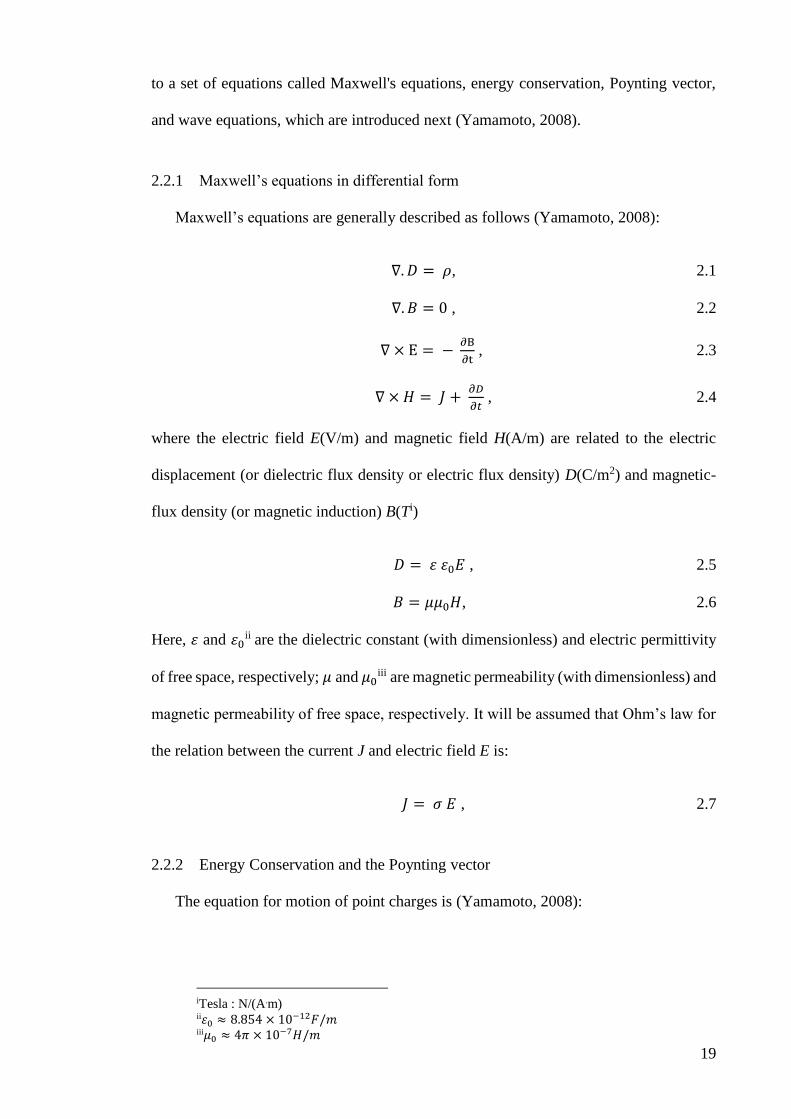
2.2.1 Maxwell’s equations in differential form
Maxwell’s equations are generally described as follows (Yamamoto, 2008):
2.1 ∇. 𝐷 = 𝜌,
2.2 ∇. 𝐵 = 0 ,
2.3 ∇ × E = − ∂B
∂t ,
2.4 ∇ × 𝐻 = 𝐽 + 𝜕𝐷
𝜕𝑡 ,
where the electric field E(V/m) and magnetic field H(A/m) are related to the electric
displacement (or dielectric flux density or electric flux density) D(C/m2) and magnetic-
flux density (or magnetic induction) B(Ti)
2.5 𝐷 = 휀 휀0𝐸 ,
2.6 𝐵 = 𝜇𝜇0𝐻,
Here, 휀 and 휀0ii are the dielectric constant (with dimensionless) and electric permittivity
of free space, respectively; 𝜇 and 𝜇0iii are magnetic permeability (with dimensionless) and
magnetic permeability of free space, respectively. It will be assumed that Ohm’s law for
the relation between the current J and electric field E is:
2.7 𝐽 = 𝜎 𝐸 ,
2.2.2 Energy Conservation and the Poynting vector
The equation for motion of point charges is (Yamamoto, 2008):
iTesla : N/(A.m) ii휀0 ≈ 8.854 × 10
−12𝐹/𝑚 iii𝜇0 ≈ 4𝜋 × 10
−7𝐻/𝑚
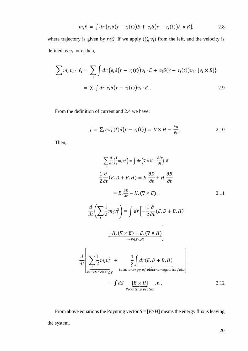
20
2.8 𝑚𝑖�̈�𝑖 = ∫𝑑𝑟 {𝑒𝑖𝛿(𝑟 − 𝑟𝑖(𝑡))𝐸 + 𝑒𝑖𝛿(𝑟 − 𝑟𝑖(𝑡))𝑟�̇� × 𝐵},
where trajectory is given by ri(t). If we apply (∑ 𝑣𝑖𝑖 ) from the left, and the velocity is
defined as 𝑣𝑖 = �̇�𝑖 then,
∑𝑚𝑖
𝑖
𝑣𝑖 ∙ 𝑣�̇� = ∑∫𝑑𝑟 {𝑒𝑖𝛿(𝑟 − 𝑟𝑖(𝑡))𝑣𝑖 ∙ 𝐸 + 𝑒𝑖𝛿(𝑟 − 𝑟𝑖(𝑡))𝑣𝑖 ∙ [𝑣𝑖 × 𝐵]}
𝑖
2.9 = ∑ ∫𝑑𝑟 𝑖 𝑒𝑖𝛿(𝑟 − 𝑟𝑖(𝑡))𝑣𝑖 ∙ 𝐸 ,
From the definition of current and 2.4 we have:
2.10 𝐽 = ∑ 𝑒𝑖�̇�𝑖𝑖 (𝑡)𝛿(𝑟 − 𝑟𝑖(𝑡)) = ∇ × 𝐻 − 𝜕𝐷
𝜕𝑡 ,
Then,
∑𝑑
𝑑𝑡(1
2𝑚𝑖𝑣𝑖
2) = ∫𝑑𝑟 (∇ × 𝐻 −𝜕𝐷
𝜕𝑡) . 𝐸
𝑖
1
2
𝜕
𝜕𝑡(𝐸. 𝐷 + 𝐵.𝐻) = 𝐸.
𝜕𝐷
𝜕𝑡+ 𝐻.
𝜕𝐵
𝜕𝑡
2.11 = 𝐸.𝜕𝐷
𝜕𝑡− 𝐻. (∇ × 𝐸) ,
𝑑
𝑑𝑡(∑
1
2𝑚𝑖𝑣𝑖
2
𝑖
) = ∫𝑑𝑟 [−1
2
𝜕
𝜕𝑡(𝐸. 𝐷 + 𝐵.𝐻)
−𝐻. (∇ × 𝐸) + 𝐸. (∇ × 𝐻)⏟ =−∇∙(𝐸×𝐻)
]
𝑑
𝑑𝑡
[
∑1
2𝑚𝑖𝑣𝑖
2
𝑖⏟ 𝑘𝑖𝑛𝑒𝑡𝑖𝑐 𝑒𝑛𝑒𝑟𝑔𝑦
+1
2∫𝑑𝑟(𝐸. 𝐷 + 𝐵.𝐻)⏟
𝑡𝑜𝑡𝑎𝑙 𝑒𝑛𝑒𝑟𝑔𝑦 𝑜𝑓 𝑒𝑙𝑒𝑐𝑡𝑟𝑜𝑚𝑎𝑔𝑛𝑒𝑡𝑖𝑐 𝑓𝑒𝑙𝑑]
=
2.12 −∫𝑑𝑆 [𝐸 × 𝐻]⏟ 𝑃𝑜𝑦𝑛𝑡𝑖𝑛𝑔 𝑣𝑒𝑐𝑡𝑜𝑟
. 𝑛 ,
From above equations the Poynting vector S = [E×H] means the energy flux is leaving
the system.

21
2.2.3 Wave equations
From 2.3 and 2.6,
2.13 ∇ × 𝐸 = −𝜇𝜇0𝜕𝐻
𝜕𝑡 ,
From 2.4, 2.5, and 2.7,
2.14 𝛻 × 𝐻 = 𝜎𝐸 + 휀 휀0𝜕𝐸
𝜕𝑡 ,
If we apply ∇ × to 2.13 and 𝜕 𝜕𝑡⁄ to 2.14 and use the relation
∇ × ∇ × 𝐸 = ∇ × ||
𝑖 𝑗 𝑘𝜕
𝜕𝑥
𝜕
𝜕𝑦
𝜕
𝜕𝑧𝐸𝑥 𝐸𝑦 𝐸𝑧
|| =|
|
𝑖 𝑗 𝑘𝜕
𝜕𝑥
𝜕
𝜕𝑦
𝜕
𝜕𝑧𝜕𝐸𝑧𝜕𝑦
−𝜕𝐸𝑦
𝜕𝑧
𝜕𝐸𝑥𝜕𝑧
−𝜕𝐸𝑧𝜕𝑥
𝜕𝐸𝑦
𝜕𝑥−𝜕𝐸𝑥𝜕𝑦
|
|
= 𝑖 [𝜕2𝐸𝑦
𝜕𝑥𝜕𝑦−𝜕2𝐸𝑥𝜕𝑦2
−𝜕2𝐸𝑧𝜕𝑧2
+𝜕2𝐸𝑧𝜕𝑥𝜕𝑧
] + 𝑗[… ] + 𝑘[… ]
= 𝑖𝜕
𝜕𝑥(𝜕𝐸𝑥𝜕𝑥
+𝜕𝐸𝑦
𝜕𝑦+𝜕𝐸𝑧𝜕𝑧) + 𝑗
𝜕
𝜕𝑦∇ ∙ 𝐸 + 𝐾
𝜕
𝜕𝑧∇ ∙ 𝐸
−𝑖∇2𝐸𝑥 − 𝑗∇2𝐸𝑦 − k∇
2𝐸𝑧
2.15 = ∇(∇ ∙ 𝐸) − ∇2𝐸 ,
If we assume ρ = 0, ∇ ∙ 𝐸 = 0, then
2.16 ∇2𝐸 = 𝜎𝜇𝜇0𝜕𝐸
𝜕𝑡+ 𝜇𝜇0휀휀0
𝜕2𝐸
𝜕𝑡2 ,
In the same way we can get
2.17 ∇2𝐻 = 𝜎𝜇𝜇0𝜕𝐻
𝜕𝑡+ 𝜇𝜇0휀휀0
𝜕2𝐻
𝜕𝑡2 ,
In case the electric field has a plane wave form:

22
2.18 𝐸 = 𝐸0𝑒𝑖(𝑘.𝑟−𝜔𝑡),
where 𝐸0 is the polarization vector, wave vector k is in the direction of the wave
propagation and the magnitude is given in 2.16.
2.19 𝑘2 = 𝑖𝜎𝜇𝜇0𝜔 + 𝜇𝜇0휀 휀0𝜔2,
In vacuum, 휀 = 1, 𝜇 = 1, 𝜎 = 0 𝑎𝑛𝑑 𝑐 𝑣⁄ = 𝜆, 𝑐 𝜔⁄ = 𝜆 (2𝜋), 𝑘 = 2𝜋 𝜆⁄ = 𝜔 𝑐 then⁄⁄
2.20 𝑐 = 1 √𝜇0휀0⁄ ,
The complex optical index �̃� may be given by
2.21 𝑘 =2𝜋
𝜆=𝜔
𝑣=�̃�𝜔
𝑐 ,
2.22 �̃�2 = 𝑘2𝑐2 𝜔2 = 𝜇휀 + 𝑖𝜎𝜇
𝜀0𝜔⁄ ,
2.23 �̃� = n + 𝑖𝑘 , 𝑘 = �̃�𝜔 𝑐⁄ = (𝑛 + 𝑖𝑘)𝜔 𝑐⁄ ,
where n and k are the real and imaginary parts of the complex optical index, respectively.
2.24 𝐸(𝑧, 𝑡) = 𝐸0𝑒−𝑘𝜔𝑧 𝑐⁄ 𝑒𝑖(𝑛𝜔𝑧 𝑐−𝜔𝑡⁄ ),
(Lambert’s law) 2.25 𝐼(𝑧) ∝ 𝐸∗𝐸 = |𝐸0|2𝑒−2𝑘𝜔𝑧 𝑐⁄ = 𝐼0𝑒
−𝛼𝑧
2.26 𝛼 = 2𝑘𝜔 𝑐⁄ ,
2.27 �̃�2 = 휀 ̃ = 휀1 + 𝑖휀2 [𝜇 = 1, 𝜎 = 0 in 2.22],
2.28 휀1 = 𝑛2 − 𝑘2, 휀2 = 2𝑛𝑘 ,
Here, α is the absorption coefficient, 휀 ̃is the complex dielectric constant, and 휀1 and 휀2
are the real and imaginary parts of the complex dielectric constant, respectively.
If we take the divergence of the plane-wave electric field,
𝑑𝑖𝑣𝐸 = (𝑖𝜕
𝜕𝑥+ 𝑖
𝜕
𝜕𝑦+ 𝑖
𝜕
𝜕𝑧) . (𝐸0𝑥𝑖 + 𝐸0𝑦𝑗 + 𝐸0𝑧𝑘)𝑒
𝑖(𝑘𝑥𝑥+𝑘𝑦𝑦+𝑘𝑧𝑧−𝜔𝑡)
= 𝑖(𝑘𝑥𝐸0𝑥 + 𝑘𝑦𝐸0𝑦 + 𝑘𝑧𝐸0𝑧) = 𝑖𝐾. 𝐸0
2.29 =𝜌
𝜀 𝜀0= 0 ,

23
It is possible to find that the electric field is a transverse wave, i.e. k⊥E0.
If the magnetic-flux density B is written as
2.30 𝐵 =𝐾×𝐸0
𝜔𝑒𝑖(𝑘.𝑟−𝜔𝑡),
then the magnetic-flux density satisfies 2.3 because
∇ × 𝐸 = 𝑖 (𝜕𝐸𝑧𝜕𝑦
−𝜕𝐸𝑦
𝜕𝑧) + ⋯
= 𝑖(𝑖𝑘𝑦𝐸𝑧 − 𝑖𝑘𝑧𝐸𝑦) + ⋯
2.31 = 𝑖𝐾 × 𝐸 ,
−𝜕𝐵
𝜕𝑡= −
𝐾 × 𝐸0𝜔
(−𝑖𝜔)𝑒𝑖(𝐾.𝑟−𝜔𝑡)
2.32 = 𝑖𝐾 × 𝐸 ,
2.3 Introduction to optics and surface plasmons
Optics is a branch of science that was developed before the knowledge of light could
be quantized into photons. Therefore, it deals with light and its manipulation at a very
broad range of wavelengths. The classical optics theory does not necessarily depend on
the fact that light is quantized into photons. Photonics, as the name suggests, also relates
to photons. It deals with aspects of light such as the generation, manipulation, and
detection of light for different purposes. It involves the wave and particle nature of light,
and is usually referred to as the technical, application-based aspect of light in areas such
as telecommunications, spectroscopy and nanocircuits (Ahmet Arca, 2010).
2.3.1 History of Surface Plasmon Resonance
Sharma et al. and Homola et al. provided a detailed history of surface plasmon
resonance (Jiřı́ Homola, Yee, & Gauglitz, 1999; Sharma, Jha, & Gupta, 2007), which is
summarized in this section with reference to the original papers. As early as 1907,
Zenneck (Zenneck, 1907) and Sommerfeld in (Sommerfeld, 1909) demonstrated and

24
formulated the existence and properties of radio frequency surface Electromagnetic (EM)
waves at the interface of a loss-free medium and a lossy dielectric, or a metal. The main
stride towards the existence of surface plasmon (SP) waves was made in 1957, when
Ritchie derived the energy distribution of a fast electron losing energy to the conduction
electrons in a metallic foil and proposed that the energy loss is due to surface plasmon
excitation (Ritchie, 1957). Ritchie’s theory was further supported by Powell and Swan
(1960) who detected the excitation of surface plasmons in aluminum and magnesium via
electrons (Powell & Swan, 1960). Their work was followed by Stern and Ferrell, who in
the same year derived the condition of resonance for surface plasmon modes and showed
that the surface waves involved electromagnetic radiation coupled to surface plasmons
(Stern & Ferrell, 1960). In 1968, Otto introduced the method of attenuated total reflection
(ATR) for resonant excitation of surface plasmon waves by light (Otto, 1968). His idea
involved using a prism near the metal vacuum interface, so that the surface plasmon
waves would be excited optically by the evanescent waves present in total reflection.
However, the most popular and widely used method to date is the Kretschmann
configuration proposed in 1968 (Kretschmann & Raether, 1968), which made the
practical and commercial use of surface plasmon resonance (SPR) possible. Instead of a
finite air gap between the prism base and metal substrate like in the Otto configuration, a
thin metal layer (10nm-100nm) remains in contact with the prism base.
The prospects of surface plasmon resonance (SPR) sensing in the field of thin film
characterization and monitoring electrochemical interfaces were further realized in work
by Pockrand et al. and Gordon et al. (Gordon Ii & Ernst, 1980; Pockrand, Swalen, Gordon
II, & Philpott, 1978). During the early 1980s, Nylander et al. and Liedberg et al.
demonstrated the use of SPR for gas detection and bio-sensing (Liedberg, Nylander, &
Lundström, 1995; Liedberg, Nylander, & Lunström, 1983; Nylander, Liedberg, & Lind,
1983). From that time onwards, the surface plasmon resonance technique has been

25
extensively utilized for the characterization and quantization of physical, chemical and
biological interactions. Since 1990, several companies have commercially launched
surface plasmon resonance biosensors (Jiřı ́Homola et al., 1999) as the Biacore instrument
(Jönsson et al., 1991). This instrument is the most accurate, sensitive, reproducible,
reliable direct SPR biosensor technique for measuring real-time biomolecular
interactions.
2.3.2 Surface plasmon concept
The surface plasmon is a traveling wave oscillation of electrons that can be excited in
the surface of certain metals with the right material properties. Because a plasmon
consists of oscillating electric charges, they also have an electromagnetic field associated
with them which also carries energy (Skullsinthestars, 2010).
Figure 2.1 A simple schematic of a surface plasmon
To explain Figure 2.1, it first may help to mention the electrical properties of electrical
conductors like metals. Electrically conductive materials have a large "pool" of electrons
within their last orbit in the atom that are essentially free to move about the material.
When an electric field is applied to the conductor, the electrons are forced into new
positions, leaving positive ions behind. The electrons tend to flow along the metal’s
surface, and the net positive charge left behind is also on the surface.

26
SPR is effectively a resonant transfer of energy from the optical excitation to the SP
wave. The fields associated with SPs decay exponentially away from the metal surface
into the dielectric, thus confining the energy onto the proximity of the metal surface.
Therefore the optical changes right next to the metal surface in the dielectric medium, or
transduction medium, modify the propagation constant of the surface plasmon and change
the SPR condition. The change in SPR condition results in changed optimum incidence
angle or wavelength for the SPR excitation. Consequently, variations in optical properties
of the dielectric medium are observed by examining the plasmon properties. SPR sensor
development dates back to the late 1970s (Jiřı́ Homola et al., 1999).
2.3.3 Surface plasmon excitation
There are two principal means of exciting SPs, namely electron bombardment or
using photons. Within the application of light two different techniques have been
developed, frustrated total internal reflection (FTIR) or attenuated total internal reflection
(ATR), and scattering by nano-sized metallic structures. Since SPs cannot be excited
directly by light waves impinging onto an ideal flat surface due to the mismatch of wave
numbers, some additional momentum must be provided to the light wave.
2.3.3.1 Excitation by Electrons
In transmission electron microscopy (TEM) or electron energy loss spectroscopy
(EELS), a beam of electrons with a well-defined and narrow range of kinetic energies
penetrates thin materials, such as metal films or specimens like living cells (Raether,
1988b). Some of the electrons are deflected due to inelastic scattering. As a result, their
paths change and kinetic energy is transferred to the sample (inter and intra band
transition or phonon and plasmon excitation). The amount of energy loss and scattering
angle can be measured in order to obtain chemical and physical data. TEM can also be
employed in such a way that the kinetic energy of the electron beam matches so that the

27
SP can be excited (Raether, 1988b). Though the newest generation of transmission
electron spectroscopy can achieve resolution of less than 1nm (Rosenauer, 2003), the
TEMs are large and very expensive to operate and probes are quite difficult to prepare.
That is primarily the reason why TEMs are not used for SP excitation.
Pfeiffer at el. (Pfeiffer, Economou, & Ngai, 1974), Martinos and Economou
(Martinos & Economou, 1981, 1983) and Ashley and Emerson (Ashley & Emerson,
1974) demonstrated theoretically that SPs can be excited on a metal cylinder by orbiting
electrons. In their models, a magnetic field oriented along the cylinder axis was applied
in order to keep the electrons around the cylinder. However, the electrons have to encircle
the cylinder on a very low orbit to excite the SPs. Another drawback is that the metal
cylinder must be very accurately shaped (Martinos & Economou, 1981). For more details
see section 2.7.1.
2.3.3.2 Excitation by Photons
In 1968, A. Otto (Otto, 1968) proposed a new technique based on frustrated total
internal reflection (FTIR) or attenuated total internal reflection (ATR) to overcome the
difficulties experienced with Electron Energy Loss Spectrometry (EELS). With this novel
approach, photons are employed to excite SPs. Ever since several configurations based
on ATR have been proposed that ensure the match between the wave numbers of the
incident light and SPs, including the Otto-Raether and Kretschmann configurations.
Similarly, other photon-based approaches are gratings and surface defects or, more
recently, pointed probes of near field microscopes.
28
Figure 2.2 (a) Kretschmann; and (b) Otto configuration of an attenuated total reflection setup for coupling
surface plasmons. In both cases, the surface plasmon propagates along the metal/dielectric interface
2.3.4 Otto and Kretschmann configurations
The Otto or Otto-Raether configuration, as depicted in Figure 2.2, consists of a prism
in close proximity to a metal surface. A laser beam is coupled at the critical angle θ into
the prism in such a way that the beam at the base of the prism, which faces the metal
surface, becomes totally reflected. Due to total internal reflection, the evanescent field
penetrates the metal surface and excites the SPs (Knoll, 1998; Zayats, Smolyaninov, &
Maradudin, 2005). If the wave number of the incident wave parallel to the interface prism-
metal matches the wave number of the SPs, a dip in reflected wave intensity can be
observed. In that event, part of the evanescent field’s energy has been transferred into the
SP; hence the name attenuated total reflection. In order to obtain good coupling efficiency
the prism must be placed very close, usually a few tens of nanometers, and aligned
parallel to the metal. However, this demands very clean and planar surfaces of both prism
and metal; consequently this configuration is not applicable for curved surfaces such as a
metal cylinder or metal sphere. This is one of the reasons why this configuration has not
been widely used (Knoll, 1998).
The Kretschmann configuration (Figure 2.9) is also based on ATR. In the simplest
form, it consists of a prism and a very thin metal film deposited on the base of the prism.
The evanescent wave, originating again from total reflection at the boundary prism-metal,

29
penetrates through the metal film and triggers surface plasmon propagation at the outer
metal interface. In addition, there is a second angle of incidence at which SPs at the
interface prism-metal film can be excited (Kretschmann & Raether, 1968).
Numerous variations based on the Kretschmann geometry have found applications in
biotechnology (Abdulhalim, Zourob, & Lakhtakia, 2008; Hutter & Fendler, 2004; Vo-
Dinh, 2008), surface science and microscopy (Novotny & Hecht, 2012; Prasad, 2004;
Raether, 1988b; Zayats et al., 2005) owing to the extraordinary sensitivity of surface
plasmon-based sensors. Even the slightest change in the permittivity of the attached film
for instance, results in strong reflected angle variation (Prasad, 2004) or a frequency shift
that can be detected (Abdulhalim et al., 2008).
However, the Kretschmann geometry can only be applied for the excitation of SPs on
planar films that are thinner than the penetration depth of the evanescent wave. Therefore,
other means have to be employed to excite SPs on optical thick metal layers or on curved
surfaces.
2.3.5 Surface plasmon polaritons
Surface plasmon polaritons (SPPs) are infrared or visible frequency electromagnetic
waves trapped at, or guided along metal-dielectric interfaces, which have shorter
wavelength than the incident light (photons). Collective charge oscillations at the
boundary between an insulating dielectric medium (such as air or glass) and a metal (such
as gold, silver or copper) are able to sustain the propagation of infrared or visible
frequency electromagnetic waves known as surface plasmon polaritons (SPP).
2.3.6 Surface Plasmon Resonance
Surface plasmon resonance (SPR) is an optical technique with applications in a
variety of disciplines, especially in sensing devices. Its popularity can be attributed to the

30
cross-disciplinary philosophy of present-day research (Chhatre, Solasa, Sakle, Thaokar,
& Mehra, 2012; Fry et al., 2011; Piliarik et al., 2012; Shalabney & Abdulhalim, 2012;
Xu et al., 2012). The SPR can be applied to probe changes in refractive index, which
often occurs within an immediate vicinity of the sensor surface. Previously, the SPR was
employed to investigate an inherent optical property of the thin metal films. Its usage has
subsequently been expanded to a multiplicity of applications including absorbance
measurements, bio-kinetics, biosensing techniques, bulk liquid measurements, immune
sensing, blood protein detection, gas detection, light modulation, process analytics,
spectrometers, microscopy, refractive index measurements, polarization fibers, and thin
film characterization (Bhatia & Gupta, 2012; Campbell & Kim, 2007; Liedberg et al.,
1983; Giancarlo Margheri et al., 2012; Naimushin et al., 2002; Schmidt, Lee, Yang, &
Harrison, 2012; Watanabe, 2011).
However, SPR has not been limited to these fields but has been employed in electrical
engineering, chemistry, theoretical physics, and experimental optics as well. The
multidisciplinary nature of SPR requires knowledge of optical waveguide, thin-film, and
optical detection techniques, besides the application under study. SPR is now widely
prevalent due to the cross-disciplinary philosophy of current research (Mcdonnell, 2001).
In sensors, the surface plasmon (SP) mode is stimulated at the interface of a thin metal
film and small dielectric layer using a light wave. A refractive index change in dielectric
medium results in altered propagation constant of the SP mode waveguide. Therefore,
this alters the condition of coupling among the propagated light wave with specific
incident angle and the SP wave, which becomes evident as a change in one of the optical
wave characteristics interacting with the SP mode. Based on their optical characteristics,
these sensors can be categorized into polarization, phase, intensity, wavelength, and
angular modulation. In this work, angular modulation was used for detection (Figure 2.4)
(J iˇrí Homola, 2006b; Jirí Homola, 2008; Oliveira et al., 2013).

31
Figure 2.3 The surface plasmon mode (wave) is excited at the interface between a metal film and
dielectric medium using a light wave
In SPR sensors with angular modulation, a monochromatic light wave excites a
surface plasmon wave. For multiple different angles of incidence of input light the
strength of coupling between the incident wave and surface plasmon wave is measured.
Figure 2.4 Concept of surface plasmon resonance sensors

32
(a)
(b)
Figure 2.5 Intensity of light wave interacting with a surface plasmon as a function of angle of incidence
In SPR sensors with wavelength modulation, a surface plasmon wave is excited by a
collimated, broad-spectrum light wave. Unlike the previous method, the angle at which
the light wave is incident onto the metal film is kept constant and the strength of coupling
between the incident wave and surface plasmon is measured for the input spectrum.
Again, the wavelength that results in the strongest coupling is considered the sensor
output (J iˇrí Homola, 2006b).
Figure 2.6 (a) Direct and (b) Indirect SPR sensors: measurand and sensor output

33
For SPR sensors with intensity modulation, the light wave intensity is deemed an
indicator of the strength of coupling between the incident light wave and a surface
plasmon mode at a single angle of incidence and wavelength (Figure 2.5). The angle of
incidence yielding the strongest coupling serves as the sensor output (Figure 2.6) and can
help determine the refractive index.
In SPR sensors with phase modulation, the shift in light wave phase interacting with
the surface plasmon is measured at a single angle of incidence and wavelength. Phase
changes are detected using the interferometry techniques and are used as the sensor
output.
In SPR sensors with polarization modulation, changes in the polarization of the light
wave interacting with a surface plasmon are measured. The last three techniques are
generally used in setups in which the light, for either surface plasmon excitation or
measurement, is carried by a waveguide.
In addition to the mentioned categorization, SPR sensors are classified as either direct
or indirect. In direct SPR sensors, the measurand (typically refractive index) directly
modifies coupling characteristics, while in indirect SPR sensors the measurand modulates
an intermediate that alters the coupling characteristics. SPR affinity biosensors are a
typical example of indirect SPR sensors (J iˇrí Homola, 2006b).
2.4 Planar Surface Plasmons
A single flat metal surface is probably the most basic metal structure to describe SP
propagation. Nevertheless, some important results can be derived with this simple
configuration. Within this section, it is assumed that the interface, which separates the
metal and dielectric, is placed on the x-z plane of a Cartesian coordinate system. It is also
assumed that the metal occupies the y < 0 region and the SPs propagate along the x-axis.
It can be demonstrated that only TM plasmons can propagate along the surface (Maier,

34
2007; Raether, 1988b; Zayats et al., 2005) because the relative permeability µ is close to
unity for most natural metals at optical frequencies (see Appendix A). There is an
alternative explanation derived from the boundary condition
2.33 (𝐷𝑑 − 𝐷𝑚) ∙ 𝑛 = 𝛿
where Dd and Dm are the dielectric displacement in the dielectric and metal, respectively,
and n is the normal vector at the interface. As a consequence of 2.33 only the components
of E in the plane of the incident wave can induce longitudinal surface charge density
oscillations in the direction of propagation (x-axis) (Knoll, 1998). The only magnetic field
component left is H, hence only TM plasmons can propagate along the metal surface. The
EM field associated with TM plasmons also decays exponentially away from the interface
into both media (Figure 2.7). Therefore, the following solution for Hy can be assumed:
2.34 𝐻𝑦 = 𝐴 ∙ 𝑒𝑗(𝜔𝑡−𝑞𝑋𝑋) ∙ exp(𝛼𝑚𝑦) 𝑦 < 0, metal
and
2.35 𝐻𝑦 = 𝐵 ∙ 𝑒𝑗(𝜔𝑡−𝑞𝑋𝑋) ∙ exp(−𝛼𝑑𝑦) 𝑦 > 0, dielectric
where A and B are amplitudes to be determined by the boundary conditions; and 𝛼𝑚 and
𝛼𝑑 are the reciprocal (positive and real) penetration depths into the metal and dielectric,
respectively. The TM-plasmon wave number 𝑞𝑥 is complex due to the presence of a metal
with the permittivity 휀𝑚 = 휀𝑚′ + i휀𝑚′′. Consequently, the amplitude of the SPs decreases
with increasing propagation distance, and eventually dissipates. The penetration depth is
defined as the distance from the interface metal-dielectric at which the amplitude of Hy is
reduced by e-1:
2.36 𝛼𝑑
𝑚= √𝑞𝑥2 − 𝑘0
2 𝜀𝑑
𝑚

35
Figure 2.7 3D model of surface plasmon propagating along a flat metal surface in the x-direction; A
snapshot of the Hy distribution (TM mode) is schematically shown. The relative permittivity 휀𝑑 is for the
dielectric material and e is for the metal. The evanescent waves in the y-direction are indicated by the
dash-dotted line.
The penetration depths and permittivities are also related (see Appendix A for
derivation) by:
2.37 −𝛼𝑑
𝜀𝑚′=𝛼𝑚
𝜀𝑑
where 휀𝑑 and 휀𝑚′ are the real permittivities of the dielectric material and metal,
respectively. From 2.36 it can also be concluded that the penetration depth of the plasmon
into the metal is much smaller than into the dielectric, as indicated in Figure 2.7. The real
part of the permittivity of the metal, 휀𝑚′, must take on negative values to satisfy 2.37,
because the penetration depths are positive real numbers by definition. The real part of
the complex wave number can then be written as (Barnes, Dereux, & Ebbesen, 2003;
Dragoman & Dragoman, 2008; Knoll, 1998; Maier, 2007; Raether, 1988b):

36
2.38 𝑞𝑥′ = 𝑘0√
𝜀𝑑𝜀𝑚′
𝜀𝑑+𝜀𝑚′
In order to obtain a positive wave number, the permittivity condition is |휀𝑚|>휀𝑑. The
imaginary part of the plasmon wave number is
2.39 𝑞𝑥′′ =
𝑘0
2(𝜀𝑑𝜀𝑚′
𝜀𝑑+𝜀𝑚′)32⁄ 𝜀𝑚′′
𝜀𝑚′2
The propagation distance of SPs along the surface is limited owing to losses in the
metal, and it is represented by the imaginary part of the permittivity 휀𝑚′′. The propagation
length L is defined as (Raether, 1988b; Zayats et al., 2005):
2.40 𝐿 = (2𝑞𝑥′′)−1
Inserting 2.39 into 2.40 yields:
2.41 𝐿 =1
𝑘0(𝜀𝑑+𝜀𝑚′
𝜀𝑑)32⁄ (𝜀𝑚′)
12⁄
𝜀𝑚′′
The propagation distance L on a flat metal surface for gold, silver and aluminum as
determined by 2.41 is depicted in Figure 2.8.
Returning to the dispersion relation 2.38, the solutions for the real part of the plasmon
wave number 𝑞𝑥 of TM plasmons on a silver surface with metal permittivity described
by the Drude-Lorentz Modeli (2.33) surrounded by vacuum is shown in Figure 2.9.
i휀𝑟(𝜔) = 1 −
𝜔𝑝2
𝜔2−𝑖𝛾𝜔 ; where 𝜔𝑝and 𝛾 are the bulk plasma frequency and damping frequency
respectively.

37
Figure 2.8 Propagation length for SPs on a planar surface for gold, silver and aluminum (Vogel, 2009)
For small wave numbers the dispersion curve of the TM plasmons (Figure 2.9, surface
plasmon polaritons) asymptotically approaches the dispersion curve of the bulk wave
(light-line) in the adjacent dielectric (Figure 2.9, free space). For large wave numbers it
approaches the SP condition 𝜔𝑠𝑝 = 𝜔𝑝/(휀𝑑 + 1)1/2, which also corresponds to the
condition 휀𝑑 = −휀𝑚(𝜔). One important result is that the free space curve does not
intersect the SPP curve, which represents the dispersion relation of the bulk wave in the
adjacent dielectric. Consequently, light waves cannot excite SPs on a flat metal surface
or SPs cannot radiate into light waves without appropriate devices, hence the term non-
radiative SPs. This is a consequence of Snell’s law, which imposes the condition that the
component of the wave vector parallel at the interface is continuous. In other words, the
wave vector of the surface plasmon and wave vector of the bulk wave do not match at the
interface; once the SPs are coupled into a smooth metal surface, they are trapped (Barnes
et al., 2003).

38
Figure 2.9 Dispersion relation of SPs on a flat Ag surface, with the permittivity of Ag modeled by Drude-
Lorentz Model; λ𝑝 is the corresponding plasmon wavelength and 휀𝑑 = 1 is the permittivity of the adjacent
dielectric material. See text for curve descriptions.
Between the bulk plasma frequency 𝜔𝑝 and surface plasmon frequency 𝜔, no solution
corresponding to SPs exists. This can also be shown by substituting Drude-Lorentz Model
(DLM) for a weakly damped system (휀𝑟(𝜔) = 1 −𝜔𝑝
2
𝜔2; when 𝛾 → 0 ) into 2.38. This
frequency gap is also known as the plasmon gap (Maier, 2007). For applied frequencies
higher than the bulk frequency 𝜔𝑠𝑝 another solution exists, where the plasmon wave
radiates in the metal (Figure 2.9, plasmon polariton) (Maier, 2007; Raether, 1988b).
However, these modes are not confined to the interface and are of no interest for this
project.
2.4.1 Surface plasmons in three-layer configuration
An important extension of a simple metal surface is a three-layer configuration, where
each of the layers has an infinite extension in two dimensions. Two basic configurations
are well-known: a dielectric gap in a metal, or metal-dielectric-metal (MDM)
configuration, and a metal film surrounded by two dielectrics, or dielectric-metal-
dielectric (DMD) configuration. However, because of the additional interface, the

39
dispersion relation becomes more complex owing to the fact that the surface plasmons on
each interface couple and form new, additional modes when the thickness of the metal
film or gap width becomes sufficiently small.
In this section it is assumed that our study adopts the dielectric-metal-dielectric
structure that extends infinitely in the x- and y- directions and the plasmon propagation
is along the x-axis. In view of the fact that only TM plasmons can propagate, the
distinction of different plasmon modes is determined by the distribution of the sole
magnetic field component Hy across the metal film (Gramotnev & Vernon, 2007;
Gramotnev, 2005).
2.4.2 Theoretical background of SPs in DMD structure
Assume an optical waveguide composed of the three homogeneous layers
(Figure 2.10) with a permittivity profile:
휀(𝑥) = 휀3 𝑥 > 𝑑,
2.42 휀(𝑥) = 휀2 − 𝑑 < 𝑥 < 𝑑 ,
휀(𝑥) = 휀1 𝑥 < −𝑑,
where d is defined the half-thickness of wave guiding layer and εi (i = 1, 2, 3) is complex
permittivity in general.
With orienting the Cartesian axes as presented in Figure 2.10, the field vectors are
only in x and z and the modal fields can be written as:
𝐸 = 𝒆(𝑥) ∙ exp(𝑖(𝛽𝑧 − 𝜔𝑡)) 2.43
𝐻 = 𝒉(𝑥) ∙ exp(𝑖(𝛽𝑧 − 𝜔𝑡))

40
Figure 2.10 Three-layer dielectric-metal-dielectric waveguide structure
Substituting the field profiles into a simplified wave equation yields for the
transversal components of the field vectors:
2.44 𝜕2𝑒𝑦(𝑥)
𝜕𝑥2+ (𝜔2휀휀0𝜇0 − 𝛽
2)𝑒𝑦(𝑥) = 0; TE modes,
2.45 𝜕2ℎ𝑦(𝑥)
𝜕𝑥2+ (𝜔2휀휀0𝜇0 − 𝛽
2)ℎ𝑦(𝑥) = 0; TM modes,
In each medium the solution of the above equations can be stated as a linear
combination of the functions: exp (𝑖𝐾𝑖𝑥) and exp (−𝑖𝐾𝑖𝑥), where 𝐾𝑖2 = 𝜔2휀𝑖휀0𝜇0 − 𝛽
2(i
= 1, 2, 3) (J iˇrí Homola, 2006b).
Outside the wave guiding layer, the fields of modal bound to a waveguide decline
exponentially through increasing distance from a waveguide. The boundary conditions of
Maxwell’s equations have a requirement that the components of electric and magnetic
field intensity vectors parallel to the boundaries of wave guiding layer which are
continuous at each boundary (x = d and x = – d). The conditions of boundary offer the
homogenous series of four linear equations for four unknown amplitudes, which yield a
non-zero solution only if the determinant of the matrix of coefficients is equal to zero (J
iˇrí Homola, 2006b). This requirement leads to the following eigenvalue equations:
2.46 tan( 𝐾𝑑) =𝛾1𝐾⁄ +
𝛾3𝐾⁄
1−(𝛾1𝐾⁄ )(
𝛾3𝐾⁄ ); TE modes,

41
2.47 tan( 𝐾𝑑) =𝛾1𝜀2
𝐾𝜀1⁄ +
𝛾3𝜀2𝐾𝜀3⁄
1−(𝛾1𝜀2
𝐾𝜀1⁄ )(
𝛾3𝜀2𝐾𝜀3⁄ )
; TM modes,
where 𝐾2 = 𝜔2휀휀0𝜇0 − 𝛽2 and 𝛾1,3
2 = 𝛽2 − 𝜔2휀1,3휀0𝜇0.
The eigenvalue equations are transcendental equations for propagation constants of
the unknown modal. Afterward that solved the eigenvalue equations, the field profiles
can be obtained by substituting the modal propagation constant values β into the boundary
conditions and computing the amplitudes.
If the media constituting the waveguide are lossless (ε1, ε2, and ε3 are real positive
numbers), the propagation constants are also real. The propagation constants of modes of
the waveguide consist of the absorbing media (e.g., metal) are complex (Jiˇrí Homola,
2006). The propagation constant is related to the modal effective index nef and modal
attenuation b as follows:
2.48 𝑛𝑒𝑓 =𝑐
𝜔𝑅𝑒{𝛽} ,
2.49 𝑏 = 𝐼𝑚{𝛽}0.2
𝑙𝑛10 ,
where Re{} and Im{} state the real and imaginary parts of a complex number,
respectively, and c presents the speed of light in vacuum; the modal attenuation b is in dB
cm–1 if β is given in m–1.
A case study of planar waveguide supporting surface plasmon is a thin metal film
placed between two semi-infinite dielectric media (Figure 2.10). If the metal film is much
thicker than the penetration depth of the surface plasmon at each metal–dielectric
interface, this waveguide supports two TM modes, which correspond to two surface
plasmons at the opposite boundaries of the metal film. When the metal thickness
decreases, coupling between the two surface plasmons occurs, giving rise to mixed
electromagnetic field modes. In this case, the metal film is gold 50nm thick.

42
The modes of a dielectric–metal–dielectric waveguide can be found by solving the
eigenvalue equation for TM modes. For any metal film thickness, there are two coupled
surface plasmons referred to as the symmetric and anti-symmetric surface plasmons
according to the symmetry of the magnetic intensity distribution (J iˇrí Homola, 2006b).
Figure 2.11 3D image of SPs propagating along a metal film (DMD structure) with (a) anti-symmetric
and (b) symmetric magnetic field distribution with respect to the middle plane

43
2.4.3 Symmetric and anti-symmetric modes of SPs in DMD structure
In 1969, Economou (Economou, 1969) conducted the first systematic study of SPs on
single as well as multilayer metal films surrounded by symmetric dielectrics. To this end,
he derived the dispersion relations for different configurations by taking the Drude-
Lorentz model into account (Economou, 1969). Burke and colleagues (Burke, Stegeman,
& Tamir, 1986) have extended the analysis of SPs in thin metal films to asymmetric
structures where the metal film is bound by two different dielectrics. They also included
a detailed discussion on the effect of dissipation on the dispersion relation and classified
all possible solutions of the dispersion relation.
The study of SPs in thin films is of practical importance because they are a basic
structure for a finite metal stripe, currently one of the most discussed and analyzed
plasmonic waveguides (Berini, 1999, 2006, 2008; Brongersma & Kik, 2007; Maier, 2007;
Shalaev & Kawata, 2006; Zourob & Lakhtakia, 2010). For instance, one of the methods
of determining the wave number is the effective index method (EIM). This approach
basically consists of decomposing the 2D waveguide structure into two 1D structures
(DMD or MDM) and matching the solution of each 1D structure. However, EIM is not
only confined to rectangular structures but is also applicable for other 2D waveguide
structures, such as grooves and gaps (Bozhevolnyi, 2006).
In DMD structure, two different film (plasmon) modes can be excited, depending on
whether the magnetic field H in the film is symmetric or anti-symmetric with respect to
the middle plane (see Figure 2.11).

44
Figure 2.12 Dispersion relation qx(h), where h is the film thickness of a DMD plasmon waveguide for
symmetric and anti-symmetric magnetic field Hy. Effective index and modal attenuation of surface
plasmons propagating along thin gold film (εm= -25 + 1.44i) slotted in between two dielectrics (nd1=1.32
and nd2= 1.35) as a function of gold film thickness; wavelength is 800nm
For a symmetric DMD structure, the metal film is bounded on each side by the same
dielectric. The dispersion relation q(h) is then given by
2.50 𝑡𝑎𝑛ℎ𝛼𝑚ℎ
2= −
𝛼𝑑𝜀𝑚
𝛼𝑚𝜀𝑑,
for the symmetric magnetic field distribution across the film (anti-symmetric charge
distribution) regarding the middle plane and
2.51 tanh𝛼𝑚ℎ
2= −
𝛼𝑚𝜀𝑑
𝛼𝑑𝜀𝑚,
for the anti-symmetric magnetic field distribution (symmetric charge distribution), where
𝛼𝑑 and 𝛼𝑚 are the reciprocal penetration depths into the dielectric and metal, respectively,
and 휀𝑑 and 휀𝑚 denote the corresponding permittivity (Gramotnev & Vernon, 2007;
Gramotnev, 2005; Vogel, 2009).

45
Thin, metal film packed amid two semi-infinite dielectric media is otherwise known
as a planar waveguide that supports surface plasmons (Figure 2.10). In case the metal
film is quite a bit thicker than the surface plasmon penetration depth at all metal–dielectric
interfaces, such waveguide sustains two TM modes related to two surface plasmons at
the metal film’s opposite bounds. With decreasing metal thickness, two surface plasmons
will connect resulting in mixed electromagnetic field modes.
It is possible to obtain dielectric–metal–dielectric waveguide modes by working out
the eigenvalue (2.47). Figure 2.11 (a) and (b) presents the eigenvalue equation’s
mathematical results with respect to symmetric waveguide configuration (nd1= nd2). For
any metal film thickness value two coupled surface plasmons are present known as
symmetric and anti-symmetric surface plasmons consistent with the magnetic intensity
distribution symmetry (Ghosh, 1998). In the symmetric surface plasmon, effective index
and attenuation both evidently amplify with thicker metal film. However, the anti-
symmetric surface plasmons’ attenuation and effective index diminish as the metal film
gets thicker. Meanwhile, for an asymmetric waveguide the symmetric surface plasmons’
effective index reduces with declining metal film thickness; at a specific thickness, the
symmetric surface plasmon stops being present in the form of a guided mode ( Figure 2.12
(c) and (d)) an occurrence known as mode cutoff. Since a symmetric surface plasmon
displays less attenuation compared to its anti-symmetric equivalent called a short-range
surface plasmon (Quail & Simon, 1984; Slavík & Homola, 2007), it is occasionally
identified as a long-range surface plasmon (Berini, 2009) (Quail & Simon, 1984; Slavík
& Homola, 2007).
Figure 2.13 shows the field vector profiles of the symmetric and anti-symmetric
surface plasmons on thin gold film surrounded by two identical dielectrics. The profiles
of magnetic intensity h of symmetric and anti-symmetric plasmons are symmetric or anti-
symmetric with respect to the center of the metal. The field of the symmetric surface
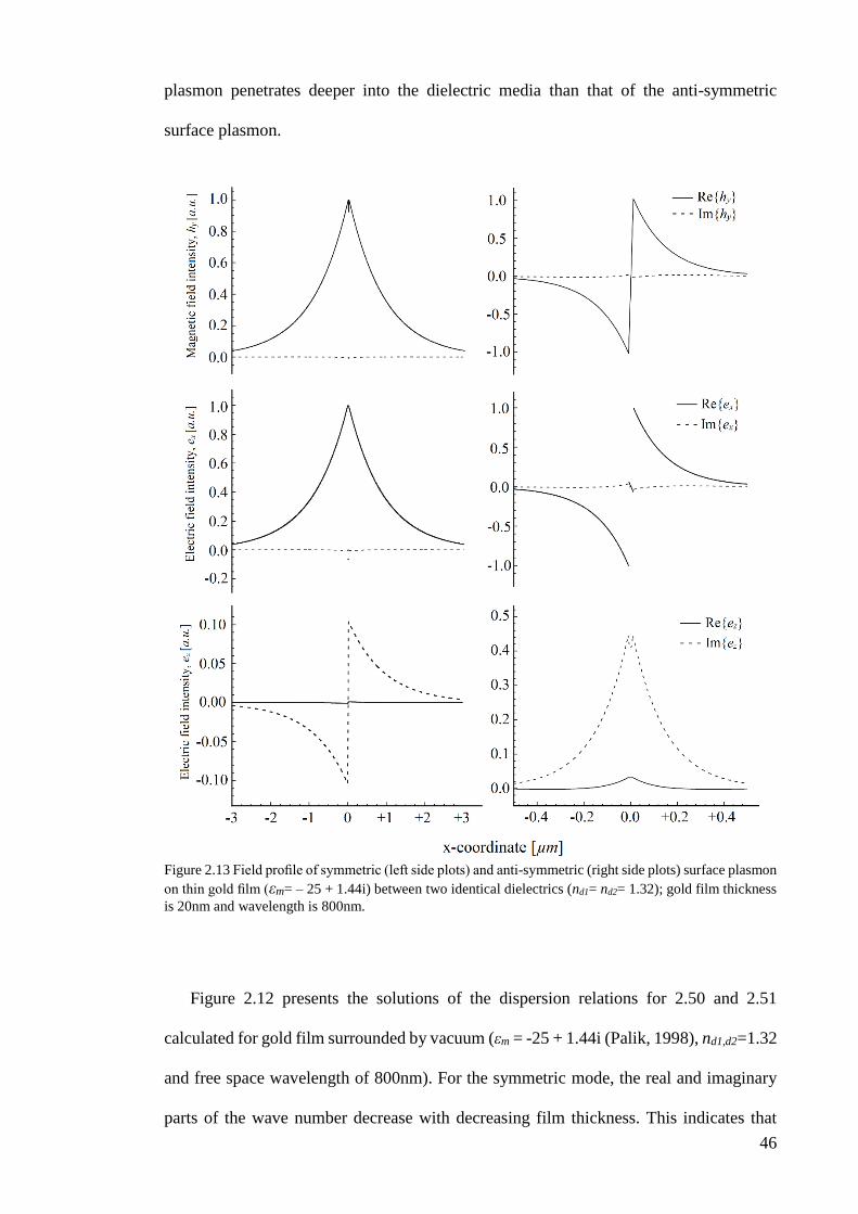
46
plasmon penetrates deeper into the dielectric media than that of the anti-symmetric
surface plasmon.
Figure 2.13 Field profile of symmetric (left side plots) and anti-symmetric (right side plots) surface plasmon
on thin gold film (εm= – 25 + 1.44i) between two identical dielectrics (nd1= nd2= 1.32); gold film thickness
is 20nm and wavelength is 800nm.
Figure 2.12 presents the solutions of the dispersion relations for 2.50 and 2.51
calculated for gold film surrounded by vacuum (εm = -25 + 1.44i (Palik, 1998), nd1,d2=1.32
and free space wavelength of 800nm). For the symmetric mode, the real and imaginary
parts of the wave number decrease with decreasing film thickness. This indicates that
47
losses are also reduced, hence according to 2.41, the propagation distance increases with
decreasing thickness. The penetration depth into the dielectric also increases and
approaches infinite distance for zero film thickness h and the symmetric plasmon
transforms into a bulk wave in the dielectric. For the anti-symmetric mode the penetration
depth decreases into the dielectric and metal, hence the localization increases with
increasing dissipation (Vogel, 2009).
The symmetric film mode in a thin metal film is also referred to as a long-range
surface plasmon polariton (LRSPP). Nevertheless, the LRSPP experiences a cutoff,
limiting the miniaturization of the metal stripe along with the problem of increasing field
localization. In practice there is always a trade-off between reasonable propagation
distances and localization (Maier, 2007). The anti-symmetric mode, on the other hand,
experiences no cutoff when the film thickness h decreases. As a result, this mode can be
employed for nanofocusing for the same reason as the MDM structure (Vogel, 2009).
If the metal film is bounded by two different dielectrics, the classification of
symmetric and anti-symmetric modes for DMD-structures, as shown above, cannot be
used without modification. For instance, a metal film is placed on a glass substrate (ε)
and surrounded by vacuum or another dielectric material (εc ≠ εs) (Burke et al., 1986;
Prade, Vinet, & Mysyrowicz, 1991). The magnetic field H is neither fully symmetric nor
fully anti-symmetric with respect to the middle plane. These modes are called quasi-
symmetric and quasi-anti-symmetric film modes (Vernon, Gramotnev, & Pile, 2007). The
dispersion relation can be derived in the same way by solving Helmholtz’s equation as
outlined in previous sections. However, due to structure asymmetry, four boundary
conditions must be considered, but more inconveniently, the dispersion relations for the
quasi-symmetric and quasi-anti-symmetric modes are expressed in one equation (Vernon
et al., 2007; Vogel, 2009).
48
Nevertheless, a method called the zero-plane method, originally developed to analyze
EM modes between two piezoelectric materials separated by a gap, simplifies the analysis
(Chernozatonskii, Ermoshin, & Gramotnev, 1991; Vernon et al., 2007). This approach
consists of subdividing the real asymmetric structure into two symmetric structures,
solving the (known) dispersion relations in both symmetric systems and then matching
the resulting solutions. The advantages are that only three boundary conditions remain
and separate equations for the two types of modes are obtained (Vernon et al., 2007;
Vogel, 2009).
The symmetric surface plasmon exhibits effective index and attenuation, which both
increase with increasing metal film thickness. The effective index and attenuation of the
anti-symmetric surface plasmon decrease with increasing metal film thickness. If the
waveguide is asymmetric, the effective index of the symmetric surface plasmon decreases
with decreasing metal film thickness and at a certain metal film thickness, the symmetric
surface plasmon ceases to exist as a guided mode. The symmetric surface plasmon
exhibits lower attenuation than its anti-symmetric counterpart and it is therefore
sometimes referred to as a long-range surface plasmon, while the anti-symmetric mode
is referred to as a short-range surface plasmon (Jiˇrí Homola, 2006).
As a key result, it will be confirmed in this section, that only TM-plasmons can
propagate along with the metal surface. In the optical and near infrared frequency
structures, the real part of the complex relative permittivity of the most of metals (gold,
silver, copper and aluminum) takes on the negative values which is a basic and mandatory
requirement for existing the surface plasmons (Palik, 1998).
2.5 Analysis methods applied in this study
In this section, the analytical and numerical methods employed throughout this PhD
study are introduced to thoroughly analyze plasmonic resonances on thin gold film. In

49
order to analytically study SPR structures, light ought to be propagated either within the
visible wavelength range (assuming the resonance occurs within this range) with a
constant SPR angle or range of incident angle with constant wavelength. Based on
analytical analysis as a mathematical method (Abarbanel & Gottlieb, 1997), the SPR
angle variation versus wavelength and the reflection intensity versus incident angle are
calculated and assessed on the SPR structure. To numerically analyze the SPR structure,
it is necessary to rely entirely on rigorous numerical methods, such as finite element
methods (FEM) (Sadiku, 2010), finite difference time domain (FDTD) (Hagness &
Taflove, 2000; Sadiku, 2010) or methods of moments (MoM) (Gibson, 2007).
2.5.1 Analytical Analysis
From a mathematical point of view, the scattering theory (also known as the field
susceptibility or Green’s dyadic technique) is based on Green’s function theory applied
to the wave equation when a source term is introduced. It simply describes the most
general analytical solution of the inhomogeneous wave equation as an integral equation
where the kernel is a Green’s function (Newton, 1982). Several electromagnetic
scattering theory formulations have been successfully applied to modeling near-field
optical phenomena. Although Green’s function may be expanded in Fourier or multi-pole
series, most formulations favor a discretization in real space since near-field optical
phenomena occur on a sub-wavelength scale (Girard & Dereux, 1996). Until now, most
analytical analyses of surface plasmon resonance have been implemented in MATLAB
software. All mathematical analysis is solved by this software according to the theoretical
description of wave equations and electromagnetic fields given in prior sections of this
chapter.
Although the surface plasmon resonance phenomenon can be modeled analytically
for bio-interaction analysis, analytically modeling a strip of metal bounded with dielectric

50
medium is not enough. Thus, for slab structure bio-interaction analysis, solving the
eigenvalue equations requires numerical calculation and cannot only be evaluated
analytically.
2.5.2 Numerical Analysis
The finite element method (FEM), or finite element analysis (FEA), is a numerical
computation technique used to obtain approximate solutions of boundary value problems
(Brenner & Scott, 2008; Garg, 2008). Simply stated, a boundary value problem (BVP) is
mathematical, whereby one or more dependent variables must satisfy a differential
equation everywhere within a known domain of independent variables and satisfy specific
conditions on the domain’s boundary. The extensive use of FEM in solving the BVP of
different disciplines has led to the production of lots of computational software such as
COMSOL Multiphysics. It is recognized for its flexibility and multidisciplinary modeling
capability.
In this work, COMSOL is employed to study of surface plasmon resonance (Ziegel,
Press, Flannery, Teukolsky, & Vetterling, 1987). COMSOL includes a powerful radio
frequency module that is suitable for analyzing optical phenomena and has been accepted
as a trustworthy result generating suit (Englebienne, Hoonacker, & Verhas, 2003; J iˇrí
Homola, 2006a, 2006b).
The physical interpretation of FEM is closely related to the method’s discovery and
extensive use in the field of structural mechanics in the early 1940s (Courant & others,
1943; Meek, 1996). The fundamental concept in the physical interpretation is the
breakdown of a complex mechanical system into simpler, disjointed components called
finite elements (Huebner, Dewhirst, Smith, & Byrom, 2008). The physical response of an
element is characterized in terms of a finite number of degrees of freedom. These degrees
of freedom are represented by values of unknown functions as a set of node points. The

51
element response is defined by algebraic equations constructed from physical or energy
specifications. The response of the original system is approximated by that of the discrete
model constructed by connecting the elements. Therefore, a physical look would indicate
that electromagnetic fields could be solved for each element and connected to form a
whole physical model by applying the correct boundary conditions and physical
approximations/assumptions. The main advantage of FEM, especially over grid-based
methods such as FDTD, is with discretization/meshing. Mesh elements in FEM can be
triangular and irregular in arrangement (Volakis, Chatterjee, & Kempel, 1998). The mesh
provides details about where every element is and to which material in the simulation
domain it associates with, and it approximates the domain’s geometrical shape. How well
the geometrical shapes are resolved in the domain contributes to the stability and accuracy
of the solution in addition to the resources used. Mesh characteristics of FEM modeling
are recognized as more efficient than conventional FDTD mesh (Garg, 2008). This is
because the non-regular triangular FEM mesh can resolve different, arbitrary, small
geometries better than the regular rectangular mesh typically employed by FDTD.
However, as emphasized throughout this thesis, FEM is applied for numerical analysis of
the SPR structure.
2.6 The application of surface plasmons in sensing
Generally, surface plasmon resonance (SPR) has a function in three major areas (Jiřı ́
Homola et al., 1999): measurement of physical quantities, chemical sensing and
biosensing. SPR sensors are utilized to measure physical quantities such as displacement
(G Margheri, Mannoni, & Quercioli, 1997) and angular position (Schaller, Czepluch, &
Stojanoff, 1997). Humidity sensors (Qi, Honma, & Zhou, 2006; Weiss, Srivastava, &
Groger, 1996) and temperature sensors (Chadwick & Gal, 1993; Turhan-Sayan & others,
2003) using SPR have been developed. In the field of chemical sensing (Jiřı́ Homola et
al., 1999), SPR is used to monitoring the distillation process (Ruiz et al., 1993), gas
52
detection (Abdelghani et al., 1997; Liedberg et al., 1983) and detecting Cu and Pb ions
(Chinowsky, Saban, & Yee, 1996; Jung, Saban, Yee, & Darling, 1996) by combining
SPR with anodic stripping voltammetry. Some of the SPR biosensing applications include
protein-protein or protein-DNA interaction assessment (Mernagh, Janscak, Firman, &
Kneale, 1998), plasma membrane examination (Kim et al., 1998), as well as DNA
detection (Goodrich, Lee, & Corn, 2004), bacteria (Koubova et al., 2001), herbicides
(Mouvet et al., 1997), and protein toxins (Ji\vr\í Homola et al., 2002).
A commercial system derived from the SPR technique has been applied to measure a
wide range of real-time bio-molecular interactions. It is possible to characterize ligand-
analyte binding reactions without labeling requirements. The incident laser light is
reflected from the inner face of the prism, which has its outer face coated by a layer of
thin noble metal film, i.e. gold in a common SPR setup. The intensity of reflected light is
lost in producing a resonance in electrons on the thin metal film at a unique angle (Berini,
2009). Since this unique angle is dependent on the refractive index of the material on the
thin metal surface, this phenomenon has therefore been applied to demonstrate molecular
interactions in solid-liquid interfaces. One reactant (a ligand) is immobilized on the gold
surface and another reactant (an analyte) flows on the gold surface. When antibodies
(Abs), acting as the analyte, and antigens (Ags) as the ligands, interact to bind each other,
the response is produced and monitored in real-time. The SPR biosensors measure the
refractive index changes in the vicinity of the immobilized surface ligands (Tanious,
Nguyen, & Wilson, 2008).
Surface Plasmon Resonance offers a new generation of label-free, real-time analysis
of bio-molecules, providing information on kinetic processes, concentration and real-time
molecule detection (Chen, Chien, Lin, & Lee, 2004; Dostálek & Knoll, 2008; Ji\vrí
Homola, 2003; Jiřı́ Homola et al., 1999; Yonzon et al., 2004). Label-free detection means
that the analyte does not need to be labeled by fluorescent molecules. A label-free, real-

53
time detection technique offers advantages over an alternative technique, such as
fluorescence-based sensors. These methods also provide high sensitivity, but they require
either multi-step detection protocols, which limit the real-time measuring ability, or suffer
from cross-sensitivity to the non-target analyte (Ji\vrí Homola, 2003), something that
reduces accuracy. The first commercial SPR application in biosensing was by Biacore
International AB in 1990 (Ji\vrí Homola, 2003). Biacore (“General Electric Company,
Biacore,” 2014) is one of the initial SPR instruments and market leaders, especially for
larger pharmaceutical companies. Companies such as Nomadics (“I. Nomadics, Sensiq
website,” 2014) and Reichert (“Reichert, Inc. , Reichert Surface Plasmon Resonance
(SPR) Systems,” 2014) also produce surface plasmon resonance sensors for real-time
binding information detection.

54
3 CHAPTER III: METHOD AND PROCEDURE
3.1 Overview
The configuration and modeling of the proposed SPR biosensor, along with
experimental method, are described in this chapter. In the first section, the four common
models of optical properties are introduced for analyzing them on SPR structure through
analytical and numerical analysis. All models have been implemented using MATLAB
programming. There is a comparison between common models and reference data in this
section as well. The reason why gold is used in this study and molecular interactions in
SPR sensors are explained in the following chapter. In addition, the dielectric-metal-
dielectric waveguide is modeled to state the dimension and optical properties of the
proposed SPR structure, which affect the surface plasmons. The molecular interactions
in modeling the SPR biosensors is briefly explained in this Chapter. The last section is
devoted to the method of our experiment. First, the simple SPR biosensor experiment is
explained and subsequently the terms and required equipment are described in detail.
3.2 Optical properties of metallic films
In order to design, and analytically and numerically study of multilayer structures
containing metal-dielectric films, accurate knowledge of the optical properties of such
films is required. The reason is that the optical properties of thin metal-dielectric are
strongly dependent on incident wavelength and film thickness. Therefore, the common
models for optical properties of thin metallic films are explained. Moreover, The
reference data of optical properties of proposed thin films in specific wavelength is stated
in following subsection.
3.2.1 Common models for optical properties of thin metallic films
The basic model in the field of optical properties of different materials is the Drude
model that almost all the other models are improvements of this model (Hertel, 2011).

55
Subsequently, few models was developed through experimentally nonparametric models
(Amotchkina et al., 2011) that was not comprehensive. The most applicable of models
based on Drude are Lorentz-Drude model (Rakic, Djurisic, Elazar, & Majewski, 1998),
Brendel-Bormann model (Rakic et al., 1998), and Multi Oscillator Model (Stenzel et al.,
1995). However, even these models are not well studied in different application
conditions. Vial and Laroche (Vial & Laroche, 2007) described the dispersion properties
of metals using Drude model versus Lorentz-Drude model. In another work (Vial, 2007),
a similar model discussion has been done by introducing two critical points in the
Lorentz-Drude model. Comparison of these models looks interesting but using a trustable
experimental data as a reference for this kind of comparing seems to be necessary to prove
the reliability of these models. Comparing nonparametric models multi-oscillator model
(Amotchkina et al., 2011) and optical properties for different metallic films (Rakic et al.,
1998) are examples of these thought. The experimental data used in this study is based
on Optical Society of America (OSA) data sheet (Schulz & Tangherlini, 1954; Schulz,
1954).
3.2.1.1 Drude model
In the most simplified cases of time domain methods which the metal-dielectric
frequency characterization is sought, the Drude model is invoked to approximate the
dispersion properties of metals:
3.1 εDrude(ω) = ε(∞) − (√f0ωp)
2
ω(ω−iΓ),
where f0 represents the oscillator strength (weight factor) and the plasma frequency ωp is
associated with intra band transitions (free-electron transitions) and is a function of
electron density and mass. Scattering frequency Γ includes all the scattering interactions
like e-e, e-phonon, and etc. However, we must consider that only limited range of
wavelength can be approximated by Drude model (Hertel, 2011).

56
3.2.1.2 Drude-Lorentz model
The Drude-Lorentz model is an improvement of Drude model by involving the
explicitly separated inters band (bound-electron effects) expression to the initial model
of Drude. By adding this Lorentzian term that is described by a semi quantum model, the
validity range of Drude model can be extended (Rakic et al., 1998).
3.2 εr,D−L(ω) = εr,Drude(ω) + ∑fj ωj
2
(ωj 2−ω 2)−i ω Γj
kj=1 ,
Where ωj and Γj are symbols of the oscillator resonant frequencies and bandwidths
respectively, k is the number of oscillators with frequency ωj, and fj is oscillator strength
or weighting factor. Despite the fact that the Drude-Lorentz model (D-L) expands the
validity range of analytical metal-dielectric constants approximations, it is not appropriate
for describing of some metals edges with sharp absorption. In some references stated that
the approximation of the Drude-Lorentz model is not well acceptable for noble metals
(Cu, Ag and Au) in the onset of inter band absorption even for five lorentzian terms
(Rakic et al., 1998).
3.2.1.3 Brendel-Bormann model
In the broadening functions such as optical parameters in the Drude model, the
Gaussian line shape functions give better results than Lorentzian line shape functions. If
the same full width at half maximum (FWHM) and same weight are assumed for both of
these functions, the Lorentzian function’s wings are usually more extended and higher
rather than the other function. As a result, all the Lorentzian based models show
immoderate absorption in spite of what is expected (Rakic et al., 1998).
The proposed model of Brendel and Bormann for solids’ dielectric function is based
on a Gaussian complex error function method (J. A. C. Weideman, 1994) to reduce the
deviance of Drude model from the real values. In this model the Lorantzian term in the
Drude-Lorentz model is replaced by the Brendel-Bormann polynomial which is improved
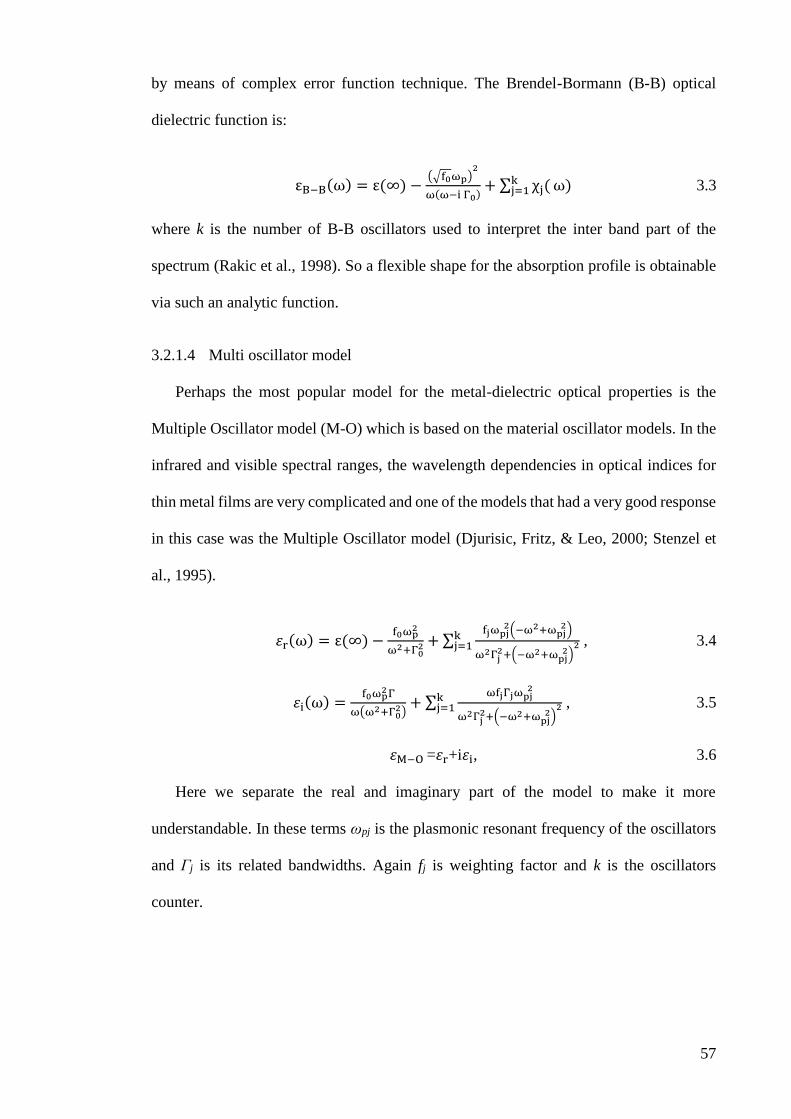
57
by means of complex error function technique. The Brendel-Bormann (B-B) optical
dielectric function is:
3.3 εB−B(ω) = ε(∞) −(√f0ωp)
2
ω(ω−i Γ0)+ ∑ χj(
kj=1 ω)
where k is the number of B-B oscillators used to interpret the inter band part of the
spectrum (Rakic et al., 1998). So a flexible shape for the absorption profile is obtainable
via such an analytic function.
3.2.1.4 Multi oscillator model
Perhaps the most popular model for the metal-dielectric optical properties is the
Multiple Oscillator model (M-O) which is based on the material oscillator models. In the
infrared and visible spectral ranges, the wavelength dependencies in optical indices for
thin metal films are very complicated and one of the models that had a very good response
in this case was the Multiple Oscillator model (Djurisic, Fritz, & Leo, 2000; Stenzel et
al., 1995).
3.4 휀r(ω) = ε(∞) −f0ωp
2
ω2+Γ02 +∑
fjωpj 2(−ω2+ωpj
2)
ω2Γj2+(−ω2+ωpj
2)2
kj=1 ,
3.5 휀i(ω) =f0ωp
2Γ
ω(ω2+Γ02)+ ∑
ωfjΓjωpj 2
ω2Γj2+(−ω2+ωpj
2)2
kj=1 ,
6.3 ,휀i+i휀r= 휀M−O
Here we separate the real and imaginary part of the model to make it more
understandable. In these terms ωpj is the plasmonic resonant frequency of the oscillators
and Γj is its related bandwidths. Again fj is weighting factor and k is the oscillators
counter.

58
3.2.2 Reference data of optical properties of proposed thin films
To prove the accuracy of each presented methods in the modeling of optical properties
of gold, the modeling simulation results should be compared with experimental data.
Since experimentally determination of refractive indices and extinction coefficients is
very difficult, the experiments on this category are so rare. However, Schulz in 1954,
published the absorption coefficients of some metals including gold (Schulz, 1954) which
is used in this study. For the refractive indices, another database which was a
collaboration of Schulz and Tangherlini is applied in this study (Schulz & Tangherlini,
1954). The measured optical constants in those datasheets have been done at the
wavelength range of 450nm to 950nm with the incidence angle of 45 degree at glass/air-
metal interfaces. Table 3.1 displays the experimental data used in this study. In this table
the refractive index and absorption coefficient is related to the proper wavelength in the
range of the modeling. The refractive index and absorption coefficient of titanium are
presented in Table 3.2.

59
Table 3.1 Refractive index (nr) and absorption coefficient (ni) of gold (Schulz & Tangherlini, 1954;
Schulz, 1954)
λ (nm) nr ni
450 1.40 1.88
500 0.84 1.84
550 0.34 2.37
600 0.23 2.97
650 0.19 3.50
700 0.17 3.97
750 0.16 4.42
800 0.16 4.84
850 0.17 5.30
900 0.18 5.72
950 0.19 6.10

60
Table 3.2 Refractive index (nr) and absorption coefficient (ni) of titanium (Schulz & Tangherlini, 1954;
Schulz, 1954)
λ (nm) nr ni
1940 3.51 5.19
1610 3.69 4.70
1390 3.67 4.37
1220 3.62 4.15
1090 3.5 4.02
984 3.35 3.97
892 3.29 3.96
821 3.21 4.01
756 3.00 4.01
704 2.86 3.96
659 2.76 3.84
617 2.67 3.72
582 2.60 3.58
549 2.54 3.43
521 2.44 3.30
496 2.36 3.19
471 2.32 3.10
451 2.27 3.04
431 2.21 3.01
413 2.14 2.98
397 2.08 2.95
381 1.99 2.93
368 1.90 2.90
354 1.82 2.87
342 1.72 2.82
332 1.61 2.74
320 1.55 2.66
311 1.50 2.57
301 1.45 2.46
292 1.40 2.36
284 1.35 2.26
276 1.30 2.17
269 1.27 2.07
262 1.27 1.99
255 1.26 1.91
249 1.27 1.83
243 1.28 1.77
237 1.30 1.72
231 1.31 1.68
226 1.32 1.66
221 1.32 1.66
216 1.32 1.67
212 1.31 1.68
207 1.31 1.69
203 1.27 1.69
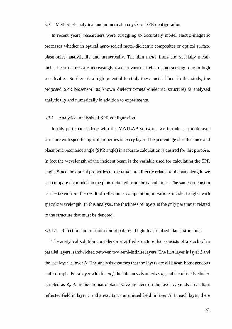
61
3.3 Method of analytical and numerical analysis on SPR configuration
In recent years, researchers were struggling to accurately model electro-magnetic
processes whether in optical nano-scaled metal-dielectric composites or optical surface
plasmonics, analytically and numerically. The thin metal films and specially metal-
dielectric structures are increasingly used in various fields of bio-sensing, due to high
sensitivities. So there is a high potential to study these metal films. In this study, the
proposed SPR biosensor (as known dielectric-metal-dielectric structure) is analyzed
analytically and numerically in addition to experiments.
3.3.1 Analytical analysis of SPR configuration
In this part that is done with the MATLAB software, we introduce a multilayer
structure with specific optical properties in every layer. The percentage of reflectance and
plasmonic resonance angle (SPR angle) in separate calculation is desired for this purpose.
In fact the wavelength of the incident beam is the variable used for calculating the SPR
angle. Since the optical properties of the target are directly related to the wavelength, we
can compare the models in the plots obtained from the calculations. The same conclusion
can be taken from the result of reflectance computation, in various incident angles with
specific wavelength. In this analysis, the thickness of layers is the only parameter related
to the structure that must be denoted.
3.3.1.1 Refection and transmission of polarized light by stratified planar structures
The analytical solution considers a stratified structure that consists of a stack of m
parallel layers, sandwiched between two semi-infinite layers. The first layer is layer 1 and
the last layer is layer N. The analysis assumes that the layers are all linear, homogeneous
and isotropic. For a layer with index j, the thickness is noted as dj, and the refractive index
is noted as Zj. A monochromatic plane wave incident on the layer 1, yields a resultant
reflected field in layer 1 and a resultant transmitted field in layer N. In each layer, there
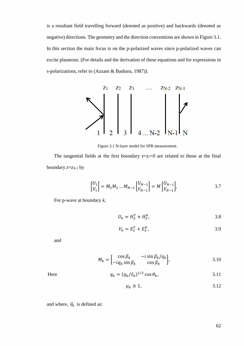
62
is a resultant field travelling forward (denoted as positive) and backwards (denoted as
negative) directions. The geometry and the direction conventions are shown in Figure 3.1.
In this section the main focus is on the p-polarized waves since p-polarized waves can
excite plasmons. (For details and the derivation of these equations and for expressions in
s-polarizations, refer to (Azzam & Bashara, 1987)).
Figure 3.1 N-layer model for SPR measurement.
The tangential fields at the first boundary z=z1=0 are related to those at the final
boundary z=zN-1 by
3.7 [𝑈1𝑉1] = 𝑀2𝑀3…𝑀𝑁−1 [
𝑈𝑁−1𝑉𝑁−1
] = 𝑀 [𝑈𝑁−1𝑉𝑁−1
],
For p-wave at boundary k,
3.8 𝑈𝑘 = 𝐻𝑦𝑇 + 𝐻𝑦
𝑅,
3.9 𝑉𝑘 = 𝐸𝑥𝑇 + 𝐸𝑥
𝑅,
and
3.10 𝑀𝑘 = [cos 𝛽𝑘 −𝑖 sin 𝛽𝑘/𝑞𝑘
−𝑖𝑞𝑘 sin 𝛽𝑘 cos 𝛽𝑘],
3.11 𝑞𝑘 = (𝑞𝑘/휀�̃�)1 2⁄ cos 𝜃𝑘, Here
3.12 𝜇𝑘 ≅ 1,
and where, kq is defined as:

63
3.13 𝑞𝑘 ≅ (1/휀�̃�)1 2⁄ cos 𝜃𝑘 =
(�̃�𝑘−𝑛12𝑠𝑖𝑛2𝜃1)
1 2⁄
�̃�𝑘,
and the phase factor is expressed by
3.14 𝛽𝑘 =2𝜋
𝜆0�̃�𝑘 cos 𝜃𝑘 (𝑧𝑘 − 𝑧𝑘−1) = (𝑧𝑘 − 𝑧𝑘−1)
2𝜋
𝜆0(휀�̃� − 𝑛1
2𝑠𝑖𝑛2𝜃1)1 2⁄ ,
in which case the design is considered by defining the arbitrary layer as thickness dk (= zk
- zk-1), dielectric constant 휀̃𝑘, and refractive index �̃�𝑘.
The interaction of the light wave and the SPP can change the characteristics of light
wave, such as the totally reflected intensity 𝑟𝑝 is:
3.15 𝑟𝑝 =(𝑀11+𝑀12𝑞𝑁)𝑞1−(𝑀21+𝑀22𝑞𝑁)
(𝑀11+𝑀12𝑞𝑁)𝑞1+(𝑀21+𝑀22𝑞𝑁),
where, 𝑀𝑖𝑗 = (∏ 𝑀𝑘𝑁−1𝑘=2 )
𝑖𝑗, 𝑖, 𝑗 = 1,2
M is the characteristic matrix of this structure which is given by
16.3 ,
kkk
kkk
kiq
qiM
cossin
/sincos
Finally, the reflectance R for the TM-polarized light of the complete multilayer structure
is described by
3.17 𝑅𝑝 = |𝑟𝑝|2,
The transmission coefficient for p-wave (TM) is
3.18 𝑡𝐻𝑝 =
2𝑞1
(𝑀11+𝑀12𝑞𝑁)𝑞1+(𝑀21+𝑀22𝑞𝑁),
3.19 𝑡𝐸𝑝 =
𝜇𝑁𝑛1
𝜇1�̃�𝑁𝑡𝐻𝑝
,
3.20 𝑇𝑝 =𝜇𝑁𝑅𝑒(�̃�𝑁 cos𝜃𝑁/�̃�𝑁
2 )
𝜇1𝑛1 cos𝜃1/𝑛12 |𝑡𝐻
𝑝|2,
For s-wave (TE) the above equations hold except
3.21 𝑞𝑘 = √�̃�𝑘
𝜇𝑘𝑐𝑜𝑠𝜃𝑘,

64
Figure 3.2 SPR curve (red line) with the BK7 galss prism|gold|air, and SPR curves (blue lines) with the
BK7 prism|gold|binding medium|air configurations.
For sensing applications, surface functionality via specific binding is necessary. This
binding results in refractive index change, which is reflected by 3.17. The binding
medium layer is clearly seen as the shift of the SPR angle as shown above.
The MATLAB program solves the mathematical calculations based on analytical
analysis which have been introduced previously, and the results will be shown in the next
chapter with comprehensive discussions.

65
3.3.2 Numerical analysis of SPR configuration
FEM is a general variational method, which finds a variational function whose
minimum/maximum/stationary point corresponds to the solution of the partial differential
equations (PDE) subject to certain boundary conditions. Its application to EM problems
can be done through the Maxwell's equations in the frequency domain. Finite element
method analysis of a problem consists of few general steps in this study which are as
follows:
Defining the required global parameters
Modeling the proposed SPR configuration in design environment
Meshing the model domain so that the simulated material is homogeneous on
each element
Deriving the governing equation for an element
Assembly of all elements into a system of equations
The solution of the system of equations based on electric/magnetic field and
power flow of structure.
A given problem is divided into many sub-problems that are easier to solve, via a
process called meshing. The problem is said to be divided into a finite number of
elements. Different shapes may be used for elements depending on the geometry to be
resolved and the computational resources available. Throughout our numerical studies in
this thesis, triangular and rectangular mesh elements (selection based on different
structures) are considered.

66
Figure 3.3 The scheme of SPR structure for numerical modeling
The SPR optical unit is composed of a source of a light beam with free space
wavelength 633nm that passes through a prism (fused silica with refractive index 1.457)
and struck the sensor surface at the angle, so that the beam is fully reflected. Under these
conditions, an electromagnetic component of the beam, the evanescent wave, spreads into
the binding medium and can interact with mobile electrons in the gold film on the glass
surface. At this incident angle and specific wavelength, the surface plasmon wave of
excited electrons is produced at the gold layer (thickness ~50nm) and is taken as a reduced
reflective light intensity at the detector. In practice, the linker, i.e. carboxymethyl dextran
matrix (thickness ~100nm) and other binding medium layers are located on top of the
gold layer, respectively.
Figure 3.3 shows the configuration of the proposed carboxymethyl dextran matrix-on-
gold surface plasmon resonance biosensor, where the gold surface is covered with a fused
silica prism. A light wave (of vacuum wavelength λ0) passes through the prism and is
totally reflected at the prism-metal interface, generating an evanescent wave. This
evanescent wave can penetrate the thin gold layer and propagate along the x direction

67
with propagation constant 𝑘𝑥 = 𝑛𝑝𝑟𝑖𝑠𝑚 (2𝜋
𝜆0) sin 𝜃1, where 𝜃1 is the light incident angle
in the first medium (prism). The propagation constant 𝑘𝑥 can be adjusted to match that of
the surface plasmon polariton (SPP) by controlling the angle of incidence. The numerical
angle change can be calculated using complex Fresnel equations based on the finite
element analysis (Englebienne et al., 2003; Verma, Gupta, & Jha, 2011).
3.4 Implementation of the proposed SPR structure
In this section, the proposed SPR configuration and all applied materials for each
layer are defined.
3.4.1 Use of gold as the metal layer
Gold and silver are the most suited metals for surface plasmon resonance sensing.
Silver has better surface plasmon resonance characteristics than gold, because of the
larger real part of its dielectric constant (Ordal et al., 1983). However, silver has poor
long-term stability. Gold is more environmentally stable, is chemically more inert, has
lower reactivity, does not react with commonly used fluids such as water and alcohols,
and is compatible with a wide range of chemicals. Thus, gold is used as the metal layer
in our studies whether analytical or numerical analysis.
3.4.2 Surface plasmons on dielectric-metal-dielectric waveguides
Structure of the model for study of surface plasmon consists of a thin metal film
surrounded with two dielectric layers, dielectric I as substrate and dielectric II as analyte;
(Figure 3.4). Assuming that the metal film is a 30nm thick gold with width of 300 nm in
our design; based on Homola’s book. The surrounding dielectric is considered to be
infinite. To analyze the structure for symmetric surface plasmon mode, the refractive
index of substrate and analyte were made equal (J iˇrí Homola, 2006b). The surface
plasmon is supported by mode analysis of its cross section for studying the capability of
this configuration. The infinite dimensions of dielectric are not practical for this
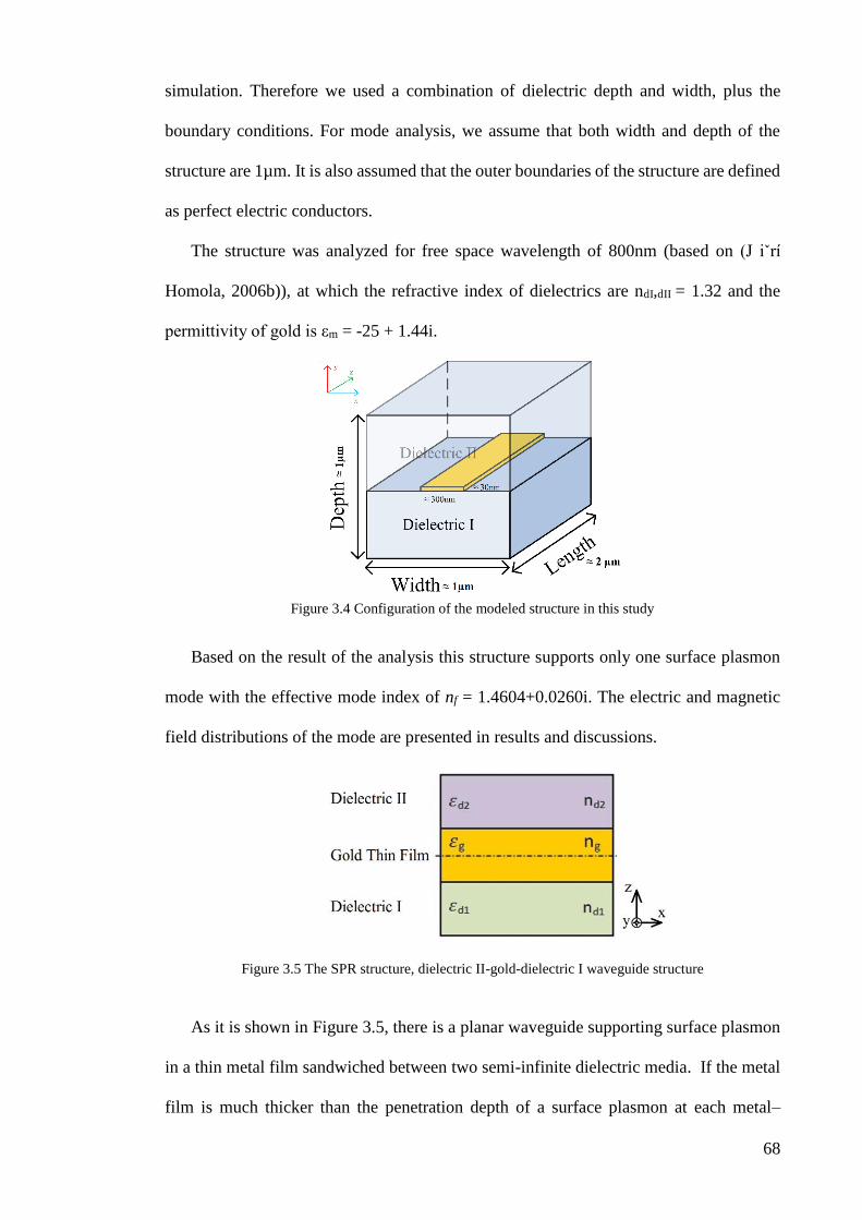
68
simulation. Therefore we used a combination of dielectric depth and width, plus the
boundary conditions. For mode analysis, we assume that both width and depth of the
structure are 1µm. It is also assumed that the outer boundaries of the structure are defined
as perfect electric conductors.
The structure was analyzed for free space wavelength of 800nm (based on (J iˇrí
Homola, 2006b)), at which the refractive index of dielectrics are ndI,dII = 1.32 and the
permittivity of gold is εm = -25 + 1.44i.
Figure 3.4 Configuration of the modeled structure in this study
Based on the result of the analysis this structure supports only one surface plasmon
mode with the effective mode index of nf = 1.4604+0.0260i. The electric and magnetic
field distributions of the mode are presented in results and discussions.
Figure 3.5 The SPR structure, dielectric II-gold-dielectric I waveguide structure
As it is shown in Figure 3.5, there is a planar waveguide supporting surface plasmon
in a thin metal film sandwiched between two semi-infinite dielectric media. If the metal
film is much thicker than the penetration depth of a surface plasmon at each metal–

69
dielectric interface, this waveguide supports two TM modes, which correspond to two
surface plasmons at the opposite boundaries of the metal film. When the metal thickness
decreases, coupling between the two surface plasmons occurs, giving rise to mixed modes
of electromagnetic field. The modes of a dielectric–metal–dielectric waveguide can be
found by solving the eigenvalue equation for TM modes. For any thickness of the metal
film, there are two coupled surface plasmons based on the symmetry of the magnetic
intensity distribution which are referred as the symmetric and anti-symmetric surface
plasmons (Jiřı́ Homola et al., 1999).
The symmetric surface plasmon exhibits effective index and attenuation, which both
increase with an increasing metal film thickness. But, effective index and attenuation of
the anti-symmetric surface plasmon decrease with an increasing thickness of the metal
film. If the waveguide is asymmetric, the effective index of the symmetric surface
plasmon decreases with a decreasing metal film thickness and at a certain metal film
thickness, the symmetric surface plasmon ceases to exist as a guided mode. The
symmetric surface plasmon exhibits a lower attenuation than its anti-symmetric
counterpart and therefore it is sometimes referred as a long-range surface plasmon, while
the anti-symmetric mode is referred as a short-range surface plasmon (Jiřı́ Homola et al.,
1999).
3.5 Molecular interactions in modeling the SPR biosensors
Binding or unbinding of biomolecules at the active surface of a SPR biosensor is one
of the most significant issues. This issue could be evaluated using analytical and
numerical analysis before experimental assessment. The determination of binding
kinetics provides important new information about interacting molecules. This is
commonly considered one of the greatest advantages of the SPR biosensor technique.
Although in ideal cases an appropriate kinetic model of molecular interaction is able to
completely describe the SPR biosensor response, in reality the influence of hydrodynamic

70
conditions often has to be taken into account. This study devotes the molecular interaction
layer in SPR configurations that correspond to the binding processes at SPR biosensor
surfaces.
As mentioned earlier, the SPR is a surface-sensitive technique that has been widely
used to monitor both chemical and biological interactions in real time, an aspect that gives
it a distinctive advantage over endpoint binding assays.
3.6 Method of experiment
In this section, all experimental parts are presented, such as how to measure the
relevant parameters of experiments, introducing the utilized equipment and solutions,
how to calculate the main output, presenting the whole steps of an assay, and sample
concentration. At the end, the samples are prepared based on the proposed concentration
for doing the experiments with an optimized sample volume.
3.6.1 A simple experiment
Consider the experimental set-up depicted in Figure 3.6. When polarized light is
shone through a prism on a sensor chip with a thin metal film on top, the light will be
reflected by the metal film acting as a mirror. On changing the angle of incidence, and
monitoring the intensity of the reflected light, the intensity of the reflected light passes
through a minimum (Figure 3.6, line A). At this angle of incidence, the light will excite
surface plasmons, inducing surface plasmon resonance, causing a dip in the intensity of
the reflected light. Photons of p-polarized light can interact with the free electrons of the
metal layer, inducing a wave-like oscillation of the free electrons and thereby reducing
the reflected light intensity.

71
Figure 3.6 Schematic fundamental set-up of SPR excitation. A biosensor with a gold film coating is
placed on a prism. The polarized light propagates from the light source on the sensor surface.
The intensity of reflected light is measured in a detector. At a certain incident angle
(𝜃), excitation of SPs occurs, resulting in a decrease of the reflected light intensity (A). A
change in optical property (refractive index) on the top surface of the gold film (termed
by sensing medium) causes a shift of angle from A to B.
The angle at which the maximum loss of the reflected light intensity occurs is called
resonance angle or SPR angle. The SPR angle is dependent on the optical characteristics
of the system, e.g. on the refractive indices of the media at both sides of the metal, usually
gold. While the refractive index at the prism side is not changing, the refractive index in
the immediate vicinity of the metal surface will change when accumulated mass (e.g.
bound antibodies to the immobilized antigens on the surface) adsorb on the surface.
Accordingly the SPR conditions are changing and the SPR angle shift is suited to take an
information on the kinetics of cell adsorption on the sensor surface.
3.6.2 Measurement of the SPR angle shift
As mentioned in chapter 2, the SPR is an accurate technique to monitor the changes
of refractive index at the near vicinity of the gold surface. Figure 3.7 shows the dip shift
in time, so-called a sensorgram. If this variation represents a biomolecular interaction,
then such interaction kinetics can be analyzed in real time.
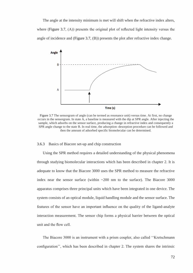
72
The angle at the intensity minimum is met will shift when the refractive index alters,
where (Figure 3.7, (A)) presents the original plot of reflected light intensity versus the
angle of incidence and (Figure 3.7, (B)) presents the plot after refractive index change.
Figure 3.7 The sensorgram of angle (can be termed as resonance unit) versus time. At first, no change
occurs in the sensorgram. In state A, a baseline is measured with the dip at SPR angle. After injecting the
sample, which adsorbs on the sensor surface, producing a change in refractive index and consequently a
SPR angle change to the state B. In real time, the adsorption–desorption procedure can be followed and
then the amount of adsorbed specific biomolecular can be determined.
3.6.3 Basics of Biacore set-up and chip construction
Using the SPR method requires a detailed understanding of the physical phenomena
through studying biomolecular interactions which has been described in chapter 2. It is
adequate to know that the Biacore 3000 uses the SPR method to measure the refractive
index near the sensor surface (within ~200 nm to the surface). The Biacore 3000
apparatus comprises three principal units which have been integrated in one device. The
system consists of an optical module, liquid handling module and the sensor surface. The
features of the sensor have an important influence on the quality of the ligand-analyte
interaction measurement. The sensor chip forms a physical barrier between the optical
unit and the flow cell.
The Biacore 3000 is an instrument with a prism coupler, also called ‘‘Kretschmann
configuration’’, which has been described in chapter 2. The system shares the intrinsic

73
phenomenon such as the direct, label-free and real-time measurement of refractive index
changes at the sensor surface.
It has ability to measure the low levels of biological and chemical compounds near
the sensor surface. Sensing of the biomolecular bindings occurs when the biomolecules
accumulate at the surface of sensor and consequently change the refractive index of
sensing medium by replacing the background electrolyte (as solutions). Antibodies have
a higher refractive index than water molecules (∆𝑛 ≈ 10−1). The sensitivity of Biacore
system is each 1000 RU corresponds to an angle change of ~ 0.1º, and 1 RU corresponds
to a refractive index change of ~1 × 10⁻⁶ of proteinous material (GE Healthcare, 2008;
Tanious et al., 2008).
According to CM5 biosensor structure (GE Healthcare, 2008), a glass surface covered
in a thin layer (~ 50 nm) of gold, providing the physical conditions for generating the
surface plasmon resonance signal. A coating on the gold layer, providing a means for
attachment of the ligand. In the case of the CM5 chip, this is a 100 nm thick
carboxymethyl-dextran matrix as a linker layer. This matrix provides a relatively inert
hydrophilic environment suitable for most biomolecular interactions. This allows
efficient immobilization from dilute solutions as well.
The SPR angle change is reported as resonance units (RU) as shown in Figure 3.8-
curve A. The Figure 3.8-curve B is calculated from the sensorgram through mathematical
calculations by MATLAB.

74
Figure 3.8 The detection approach of Biacore SPR setup. The SPR reaction is correlated to refractive
index changes at the surface of biosensor, caused by changing concentration of the binding medium when
the antibodies as a target bind to the immobilized antigens as a probe
3.6.4 Buffer Solutions for measuring the analysis cycle
3.6.4.1 Baseline buffer
The running, background or baseline buffer should create optimal conditions for the
binding of the ligand to the analyte. For biomolecular interactions the baseline buffer is
usually a physiological buffer with sufficient salt and (near-) neutral pH. Phosphate-
buffered saline (PBS) is a standard baseline buffer. Alternatively, 10 mM HEPES–KOH
(pH 7.4), 0.15 M NaCl is often used. The addition of a surfactant, e.g. Tween 20 (0.03–
0.05%) to the buffer is favored in order to minimize non-specific binding. The surfactant
not only enhances the ratio between specific and non-specific binding but also helps to
prevent air bubble adsorption on the surface. However, surfactants should not be added
if hydrophobic surfaces are used for non-covalent attachment of membrane bound
components. Moreover, a surfactant should not be used during the immobilization cycle.
Sometimes 3 mM EDTA is added to trap remaining bivalent cations (e.g. 𝑀𝑔2+ or 𝐶𝑎2+),
which may interfere with the carboxylate groups in the hydrogel layer. Blocking
components may help in reducing non-specific binding, e.g. 3% BSA or HSA when

75
patient serum is used. All buffer solutions should be prepared with Milli-Q water and
preferably filtered through a 0.22 mm filter and degassed before use.
3.6.4.2 Required solutions during an assay
N-hydroxysuccinimide (NHS) and N-ethyl-N-(dimethylaminopropyl) carbodiimide
(EDC) solutions (from amine coupling kit) are used to activate the surface of biosensor
before injection of the ligand. Deactivation and further washing away of loosely
associated ligands are performed with ethanolamine solution with pH 8.5. The 10 mM
sodium acetate buffer with a pH 4.5 is used to dilute the analyte to have sufficient
concentration for the assay process.
3.6.4.3 Regeneration solution
For repeated use of the same sensor chip, the surface should be regenerated by removal
of analyte and any other non-covalently bound material. However, the ligand should be
kept intact and should not be inactivated or denatured during the regeneration phase.
Commonly used solutions for regeneration include low pH buffers, e.g. 10 mM glycine–
HCl (pH 2.0). Optimal sensor regeneration includes a pH shock and regeneration is
preferably performed as two consecutive steps of, for instance, 30 s each, rather than one
step of 60 s. If the ligand or analyte cannot withstand low pH, sometimes a high alkaline
pH is used, e.g. 10 mM NaOH (pH >11). Alternative regeneration solutions have a high
salt concentration and the salts used include chaotropic agents that are chemicals, such as
urea and guanidine hydrochloride, that disrupt hydrogen bonding in aqueous solutions.
3.6.5 From surface plasmon to SPR signal
Real-time and label-free biomolecular interaction sensing is unthinkable at present
without the surface plasmon resonance principle. The SPR technique, liquid handlings
and the sensor chip are integrated in the Biacore 3000 as depicted in Figure 3.9.

76
Figure 3.9 Biacore 3000 system with controller unit
As discussed in Chapter 2, the SPR causes an intensity decrease or dip in the reflected
light at the sensor surface. In the following, the relationship between the intensity
decrease in reflected light and sensorgram curve are illustrated. In Figure 3.10, a
sensorgram of analyte binding versus time is presented, together with a rotated view of
an SPR dip. While the SPR angle is the most representative parameter of the biomolecular
interaction process in time, one should follow the angle of the SPR minimum (dip). As
the dip shifts in the left section from A to B, the SPR dip is followed in the right section
of Figure 3.10. The angle shift as a function of time is also shown.
Figure 3.10 Rotated presentation of the SPR dip (left section) that forms directly the pointer of the
sensorgram (right section). The angle shift of the SPR dip is determined (left, A to B), followed by
plotting the angle of the SPR minimum in the sensorgram vs. time (right). Here the SPR dip minimum of
the initial curve (A) shifts with time towards a larger angle (B).

77
Usually, the SPR curve is measured or fitted and the angle of the SPR dip is determined,
followed by plotting the angle of the SPR minimum in the sensorgram (right part of
Figure 3.10). A sensorgram can be obtained from a monochromatic light source using the
SPR dip shift (y-axis in RU or millidegrees), as shown in Figure 3.10.
From the theory described in Chapter 2, the amount of biomolecules accumulated in
the evanescent field results in an (almost) linear shift of the SPR dip. Therefore, only real-
time measurement of the SPR dip as indicated in Figure 3.10 is the preferred mode of
operation. Reflectivity change is only a derivative parameter of this shift. Therefore,
optimally the SPR dip shift should be detected continuously to follow changes at the
surface, e.g. a biomolecular interaction event. The angle shift expresses in response units
in the Biacore 3000.
3.6.6 Cycle of virus detection using scanning SPR imaging
In our study, the instrument for biomolecular interaction sensing by imaging SPR
(Biacore 3000) is used for rapid diagnostic test of dengue fever. Fixed-angle instrument
in the Kretschmann configuration (as discussed in chapter 2) are based on the relationship
between a small change in the intensity of the reflected light and the mass of bound
analyte, i.e. a fixed incident light angle is employed and mass changes are estimated from
the intensity of the reflected light. However, the applicable dynamic range and linear
relationship of this experimental setup are limited and the optimal incident angles of each
spot of a microarray differ considerably when ligand or analyte panels with different
molecular weights are monitored, as explained in Chapter 2. Therefore, choosing one
fixed angle to monitor many biomolecular interactions in a microarray will result in only
qualitative data. Kinetic rate constants, however, require accurate quantitative data
including subtraction of ‘‘bulk effects’’ for all the spots of the microarray simultaneously.

78
Biacore 3000 consists of a processing unit with liquid handling and optical systems
and a PC running Biacore 3000 Control Software. Sensor chips and other consumables
are available from GE Healthcare. As shown in Figure 3.11, Biacore 3000 processing unit
houses the following components:
two liquid delivery pumps, one for maintaining a constant flow of liquid over
the sensor chip surface and the other for handling samples in the autosampler
the autosampler, for preprogrammed sample handling including mixing and
injection to the detector unit as well as sample recovery
the Integrated µ-Fluidic Cartridge (IFC), containing liquid delivery channels,
sample loop and valves
the detector unit , including optical and electronic components for creating
and measuring SPR response
4 detector flow cells formed by the IFC pressing against the sensor chip
microprocessors for controlling pumps, autosampler and IFC valves, and for
basic processing of the SPR signal.
The removable sensor chip is inserted into the cassette port on the detector unit, and
docks into the instrument to form one side of the detector flow cell. The IFC is connected
to the buffer supply through the connector block, which has an injection port for loading
samples into the IFC.
The door to the autosampler and buffer compartment is locked during instrument
operation, to protect the operator from injury by the moving needle of the autosampler.
The instrument cannot be operated with the door open.

79
Figure 3.11 The liquid delivery system with two pumps and an autosampler transports liquid to the
connector block where samples and buffers are injected to the IFC. The scheme adapted from ref. (GE
Healthcare, 2008).
The Biacore 3000 system is used to implement the proposed SPR technique. One of the
most widely used chips for various detections in microbiological fields is CM5. Its
operating principle is based on SPR technique and is a good choice for the experiments
in this study. The approach is capable of assessing the deviation of SPR angle following
detection of anti-dengue virus immunoglobulin M antibodies (IgM) in human serum
samples.
3.6.7 Measurement of the analysis cycle: scanning SPR microarray imaging of
autoimmune diseases
3.6.7.1 Introduction
Almost every SPR-experiment applies the same basic procedure in which the first step,
the so-called immobilization (stated in next section), involves covalent binding of a ligand
to the surface of the sensor followed by the so-called analysis cycle. In order to detect the
presence or a specific interaction of a certain analyte in a sample, prior to analysis, a
capturing entity (the ligand) should be immobilized on the sensor surface. Although the
ligand can be any type of (bio)molecule, more than 80% of the capturing agents used in
SPR analysis are related to proteins (e.g. antibody, antigen, receptor, peptide). In the
previous chapter, various chemical protocols are given for the attachment of ligands to
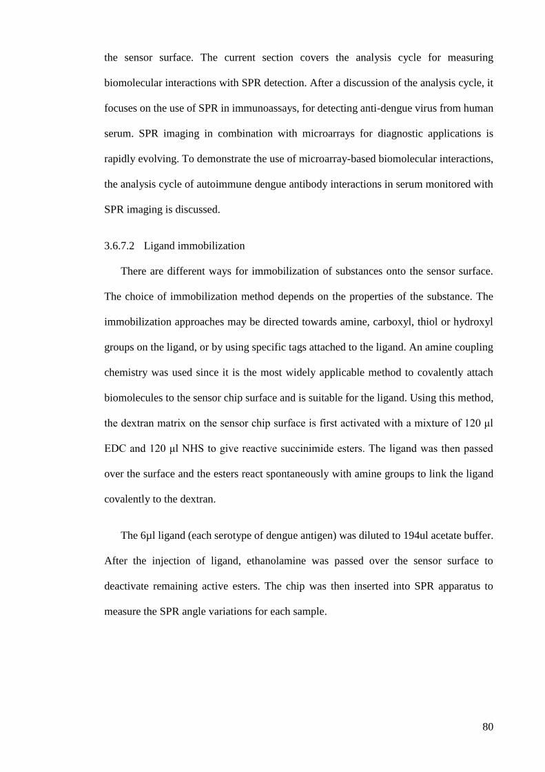
80
the sensor surface. The current section covers the analysis cycle for measuring
biomolecular interactions with SPR detection. After a discussion of the analysis cycle, it
focuses on the use of SPR in immunoassays, for detecting anti-dengue virus from human
serum. SPR imaging in combination with microarrays for diagnostic applications is
rapidly evolving. To demonstrate the use of microarray-based biomolecular interactions,
the analysis cycle of autoimmune dengue antibody interactions in serum monitored with
SPR imaging is discussed.
3.6.7.2 Ligand immobilization
There are different ways for immobilization of substances onto the sensor surface.
The choice of immobilization method depends on the properties of the substance. The
immobilization approaches may be directed towards amine, carboxyl, thiol or hydroxyl
groups on the ligand, or by using specific tags attached to the ligand. An amine coupling
chemistry was used since it is the most widely applicable method to covalently attach
biomolecules to the sensor chip surface and is suitable for the ligand. Using this method,
the dextran matrix on the sensor chip surface is first activated with a mixture of 120 μl
EDC and 120 μl NHS to give reactive succinimide esters. The ligand was then passed
over the surface and the esters react spontaneously with amine groups to link the ligand
covalently to the dextran.
The 6µl ligand (each serotype of dengue antigen) was diluted to 194ul acetate buffer.
After the injection of ligand, ethanolamine was passed over the sensor surface to
deactivate remaining active esters. The chip was then inserted into SPR apparatus to
measure the SPR angle variations for each sample.

81
Figure 3.12 Schematic of the dengue virus diagnosis process-ligand immobilization part
The optimal level of immobilized ligand depends on the purpose of the analysis. In
our case, the ligand was immobilized on the gold surface to act as a probe on the surface
of the chip. The EDC/NHS was used for activation of sensor surface (see Figure 3.12,
step 1). After surface activation, there is attraction and covalent coupling of the ligand,
and then a buffer was used to wash away loosely associated ligand (Figure 3.12, step 2).
The response level at this point provides the first indication of the immobilized amount.
Deactivation and further washing away of loosely associated ligand were performed using
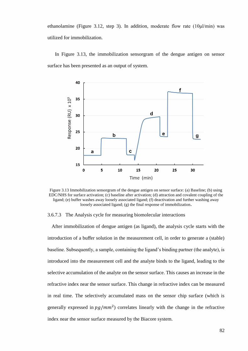
82
ethanolamine (Figure 3.12, step 3). In addition, moderate flow rate (10μl/min) was
utilized for immobilization.
In Figure 3.13, the immobilization sensorgram of the dengue antigen on sensor
surface has been presented as an output of system.
Figure 3.13 Immobilization sensorgram of the dengue antigen on sensor surface: (a) Baseline; (b) using
EDC/NHS for surface activation; (c) baseline after activation; (d) attraction and covalent coupling of the
ligand; (e) buffer washes away loosely associated ligand; (f) deactivation and further washing away
loosely associated ligand; (g) the final response of immobilization.
3.6.7.3 The Analysis cycle for measuring biomolecular interactions
After immobilization of dengue antigen (as ligand), the analysis cycle starts with the
introduction of a buffer solution in the measurement cell, in order to generate a (stable)
baseline. Subsequently, a sample, containing the ligand’s binding partner (the analyte), is
introduced into the measurement cell and the analyte binds to the ligand, leading to the
selective accumulation of the analyte on the sensor surface. This causes an increase in the
refractive index near the sensor surface. This change in refractive index can be measured
in real time. The selectively accumulated mass on the sensor chip surface (which is
generally expressed in 𝑝𝑔/𝑚𝑚2) correlates linearly with the change in the refractive
index near the sensor surface measured by the Biacore system.

83
3.6.8 The whole process of an assay
Based on the SPR technique, analyte (dengue antibodies which are in sample) is
captured by the ligand (Figure 3.14). The ligand (dengue antigens) is permanently
immobilized on the surface of sensor as explained previously.
The SPR device generates a sensorgram (RU via time) for each experiment, which
measures the response in terms of resonance units (RU) and is proportional to the
molecular mass on the surface. For an interactant of a given mass, the response is
proportional to the number of molecules at the surface. A sensorgram gives a plot of
response against time, showing the progress of the interaction and can be monitored in
real-time throughout the analysis. The results from Biacore machine were then converted
to show intensity via incident angle graph where 1000 RU is equivalent to 0.1 angle
variations.
As shown in Figure 3.14 (step 4), the dengue antibodies bind to immobilized antigens
on the gold surface. The binding interaction between the Ags and Abs was monitored by
changing the SPR angle in real-time.
Biacore 3000 was used to investigate SPR angle changes to identify the existence of
anti-Dengue virus IgM in samples. The Biacore data (Figure 3.14, step 5) was converted
to the intensity via incident angle (Figure 3.14, step 6) using MATLAB programming to
monitor the SPR angle variations. The sensor surface was regenerated at the end of each
experiment to remove the bound analyte from the immobilized ligand on the surface
(Figure 3.14, step 7).

84
Figure 3.14 Schematic of the dengue virus diagnosis process-virus detection part
Figure 3.15 presents the measurement cycles of a sensor signal using direct-detection.
Each measurement begins with conditioning the surface of sensor with an adequate buffer
solution (Figure 3.15, part 1). It is of vital relevance to have a reliable baseline before the
capturing event starts. At this point, the sensor surface contains the active ligands, ready
to capture the target analytes. On injecting the solution containing the analytes
(Figure 3.15, part 2), they are bound on the surface through its relevant immobilized
ligands. Besides, other particles of the sample might stick to the surface of sensor which
are not its relevant analyte of immobilized ligand, these binds will be non-specific, and
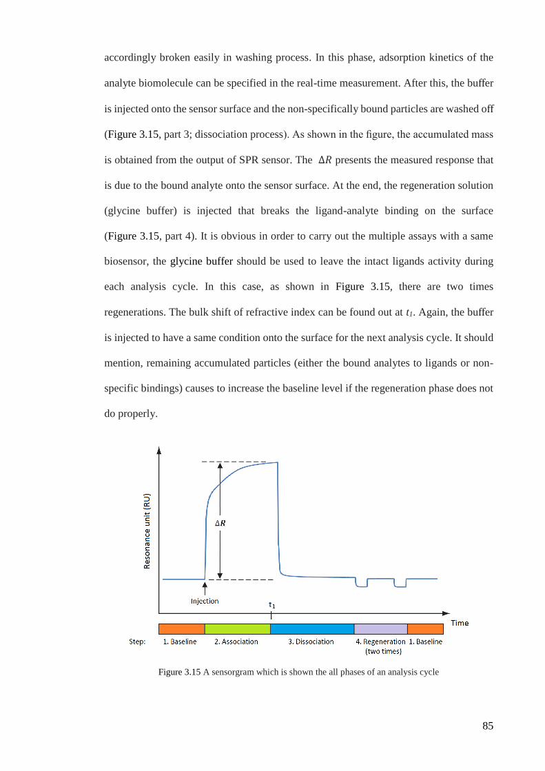
85
accordingly broken easily in washing process. In this phase, adsorption kinetics of the
analyte biomolecule can be specified in the real-time measurement. After this, the buffer
is injected onto the sensor surface and the non-specifically bound particles are washed off
(Figure 3.15, part 3; dissociation process). As shown in the figure, the accumulated mass
is obtained from the output of SPR sensor. The ∆𝑅 presents the measured response that
is due to the bound analyte onto the sensor surface. At the end, the regeneration solution
(glycine buffer) is injected that breaks the ligand-analyte binding on the surface
(Figure 3.15, part 4). It is obvious in order to carry out the multiple assays with a same
biosensor, the glycine buffer should be used to leave the intact ligands activity during
each analysis cycle. In this case, as shown in Figure 3.15, there are two times
regenerations. The bulk shift of refractive index can be found out at t1. Again, the buffer
is injected to have a same condition onto the surface for the next analysis cycle. It should
mention, remaining accumulated particles (either the bound analytes to ligands or non-
specific bindings) causes to increase the baseline level if the regeneration phase does not
do properly.
Figure 3.15 A sensorgram which is shown the all phases of an analysis cycle

86
In Figure 3.16, the data management of each assay is presented schematically from
the Biacore machine till obtaining an intensity versus incident angle graph.
Figure 3.16 Schematic of data management of each assay
3.6.9 Sample Collection
Blood samples which is used in this study were collected from University Malaya
Medical Centre, Hospital Ampang and Hospital Tengku Ampuan Rahimah (Klang). The
approval of this study protocols was accepted by the institutional review board of the
University of Malaya Medical Centre (Ethics no. 782.90) and from both Klang and
Ampang Hospital (Ethics no. NMRR-10-683-6420). Written informed consent from
patients and asymptomatic donors were obtained prior to blood collection, and the study
was conducted in accordance with the “Declaration of Helsinki”.
3.6.10 Investigation of sample concentration - calibration curve
The basic understanding of the SPR signal and the measurement procedure were
discussed in the previous section. According to the POC tests, the sample volume and
biochip surface regeneration are two significant issues which have effect on the quality
Ex
po
rt senso
rgram
Biacore control
Software
Data acquisition
xxx.txt
xxx.xlsx
Convert to excel
Mathematical analysis
through MATLAB
Intensity-Angle
graph

87
and accuracy of microbiological laboratory results. In the following, we are going to
discuss on the sample concentration with chip regeneration.
In this experiment, the different concentrations of sample are studied to determine the
most appropriate concentration to obtain highest sensing and better surface regeneration.
Evaluating the kinetic and equilibrium situations’ concentration dependence leads to
sample volume optimization under this study’s particular conditions. This experiment is
repeated under the same conditions, whereby all environmental variables (e.g.
temperature and buffers) are fixed to examine the sample concentration. The serum is
diluted (by adding solvent 10 mM sodium acetate with pH 4.5) to concentrations of 1:25,
1:50, 1:100, 1:200, 1:400 and 1:800 by adding 10mM sodium acetate solvent with pH
4.5. The experiment is carried using these six different concentrations. According to the
flow chart in Figure 3.17, we have already immobilized the serotype 2 of dengue virus
(the ligand) on sensor surface and specified patient’s serum as an analyte in different
concentrations.
Figure 3.17 Flow chart of the test concentration and regeneration of biosensor.

88
3.6.11 Clinical samples
The clinical samples were provided by University of Malaya Medical Center
(UMMC). The distinction of dengue specific IgM from cross-reactive IgM and the IgM
reactions against the infection of serotypes, which are higher than other serotypes of most
major dengue virus infection, are the primary causes of using dengue specific IgM
antibody as a target for detection.
According to Figure 3.18, the samples include:
Highly positive (antibody titre 1280-10240 or more),
Mid positive (antibody titre 160-640), and
Low positive (antibody titre 10-160),
which were classified via hemagglutination inhibition (HI) antibody and ELISA tests
(Organization & others, 2011; Peeling et al., 2010).
Figure 3.18 The samples from four different serotypes of dengue virus which have been categorized to
the three groups
Furthermore, some samples with
tick-borne encephalitis (TBE) virus,
and hepatitis C (HC) virus,

89
were provided in conjunction with the specificity investigation as shown in Figure 3.19.
The samples were tested with the SPR method to ensure high sensitivity and specificity.
Figure 3.19 Some samples with tick-borne encephalitis (TBE) and hepatitis C (HC) antibodies

90
4 CHAPTER IV: RESULTS AND DISCUSSIONS
4.1 Introduction
According to our studies in chapter 3, there are a variety of results including the
simulation and experimental works. The first section presents the mode analysis of
general SPR configuration along with the propagation analysis in symmetric mode. In the
following different optical properties models are compared in order to choose the most
appropriate model for analyzing the proposed SPR structure analytically and numerically.
The sensor signal of immobilization process is shown for all four types of dengue
virus. This sensor signal can validate the immobilization process. Furthermore, the
immobilized particles on the chip surface can be observed by microscopic images. The
determination of appropriate levels of sample concentration is a prior to examination of
all samples in our study. All samples are examined and subsequently the SPR angle
variation is obtained for each sample in order to determine the ratio of all dengue
serotypes. The sensitivity and specificity are inferred through these experimental results.
At the end, according to the samples serotype 2 which contain low, mid, and high positive
dengue viruses, the calculated SPR angle variations are investigated and then validated
through the obtained experimental SPR angle variations.
4.2 Mode and propagation analysis of general SPR configuration
In this section, the proposed SPR structure is simulated for its capability in supporting
surface plasmon wave in mode and propagation analysis of symmetric SPPs.
4.2.1 Mode analysis of symmetric SPPs
Mode analysis of cross section shows the possibility of only one surface plasmon
mode being supported with an effective index near to the dielectric material refractive
index (Figure 4.1).

91
Figure 4.1 Mode analysis of the proposed structure. (a) Mesh structure near and within the metal strip. (b)
Total energy density time average. (c-h) fields distributions: Hx, Hy, Hz, Ex, Ey, and Ez respectively
4.2.2 Propagation analysis of symmetric SPPs
Following the successful mode analysis of the structure as shown in Figure 4.1, the
three dimensional configuration of the proposed model was designed to present the

92
propagation of surface plasmon wave. The 3D structure consists of the same metal film
with length of 2µm as shown in Figure 3.4.
The boundaries were modeled using scattering boundary condition. The x and y
components of magnetic field are used to excite the wave at the input facet. A careful
meshing procedure is followed to produce a smooth result. The mesh and results are
illustrated in Figure 4.2 which shows the propagation of light along the metal strip in
terms of its electric and magnetic fields. As depicted by the figures, the power of light is
carried by the same surface plasmon mode that was obtained in mode analysis of the cross
section. It is inferred from the results that the main and the only mode for transporting
the power of light along the propagation axis, is the surface plasmon mode obtained in
the mode analysis.

93
Figure 4.2 Three dimensional simulation of the proposed model. (a) Mesh structure. (b) Energy density
time average distribution of the light. (c-h) Field distributions.
4.3 Numerical analysis for surface binding affinity
The SPR biosensor and its behavior are simulated by a numerical approach using
finite element method. The magnetic field in the z direction of plasmons on the gold film
is simulated in Figure 4.3. An increase in the z component of magnetic field (generated
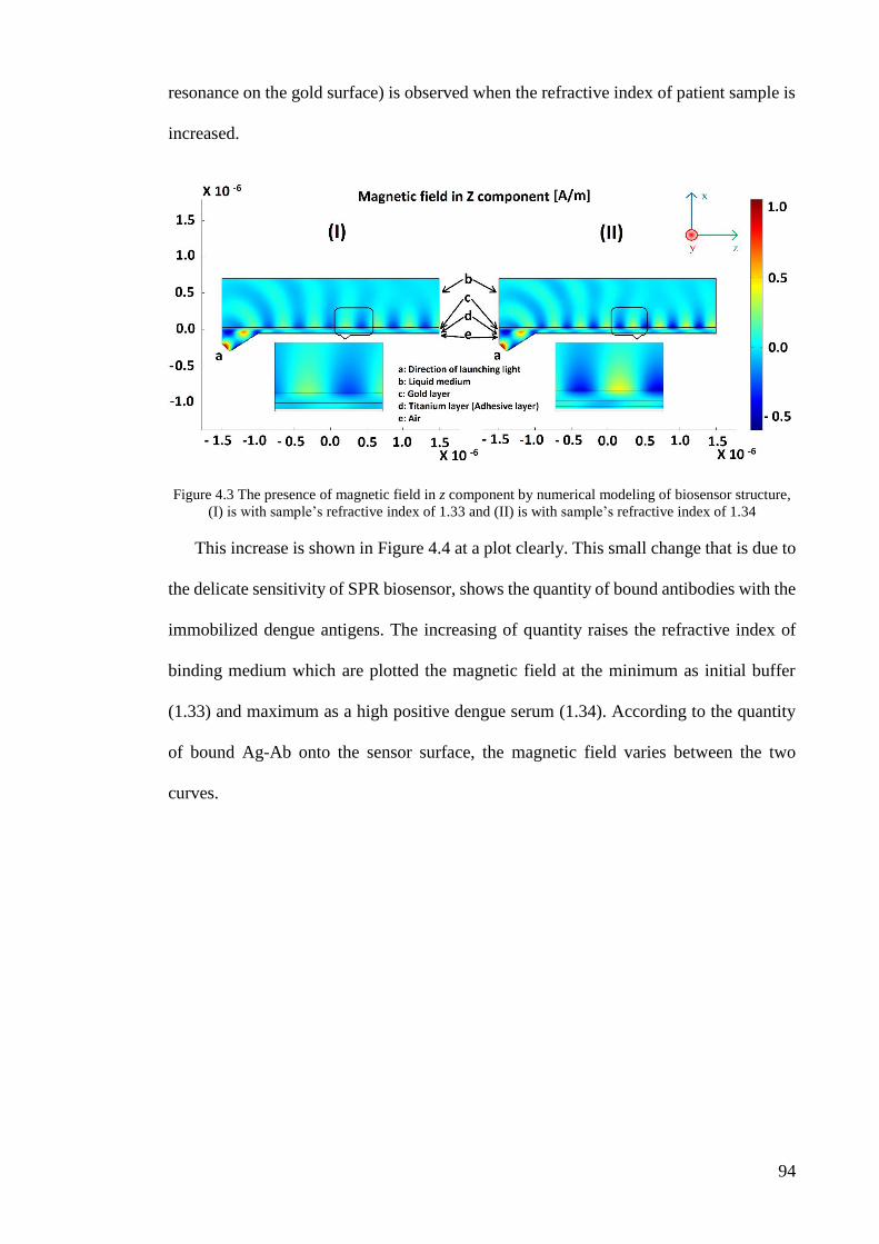
94
resonance on the gold surface) is observed when the refractive index of patient sample is
increased.
Figure 4.3 The presence of magnetic field in z component by numerical modeling of biosensor structure,
(I) is with sample’s refractive index of 1.33 and (II) is with sample’s refractive index of 1.34
This increase is shown in Figure 4.4 at a plot clearly. This small change that is due to
the delicate sensitivity of SPR biosensor, shows the quantity of bound antibodies with the
immobilized dengue antigens. The increasing of quantity raises the refractive index of
binding medium which are plotted the magnetic field at the minimum as initial buffer
(1.33) and maximum as a high positive dengue serum (1.34). According to the quantity
of bound Ag-Ab onto the sensor surface, the magnetic field varies between the two
curves.

95
Figure 4.4 Numerical analysis of biosensor structure with refractive index 1.33 to 1.34
4.4 Investigation of optical properties models on SPR structure
The common optical properties models are compared in the real and imaginary parts
of the permittivity with an experimental data and then the best model (based on the
desired range of wavelength) is applied to study the proposed SPR structure analytically
and numerically.
Here, MATLAB programming is used for mathematical analysis of SPR method to
investigate the reflectance against incident angle and SPR angle against wavelength. The
numerical part is an application for the chosen model which is simulated by COMSOL
Multiphysics.
4.4.1 Comparison between common optical properties models for metallic thin films
Following the decision to use gold as the metal thin film discussed, the permittivity
of the gold is computed at different wavelengths. For every model the real and imaginary
parts of permittivity are calculated in the separate process and compared each part from
the different models. Through an overlay plot depicted in Figure 4.5, the real part of
permittivity versus wavelength of experimental data, and Multi Oscillator, Drude-

96
Lorentz, Brendel-Bormann, Drude models are demonstrated. The error analysis with
respect to experimental data was also done (Figure 4.6).The similar overlay plot was
provided for the imaginary part of every model as shown in the Figure 4.7. In Figure 4.5
and Figure 4.7, the red dotted line represents the experimental values. The yellow, blue,
green and purple lines are representative of the Drude, Lorentz-Drude, Brendel-Bormann
and Multiple Oscillator Models respectively. It is obvious that the Drude model has the
least agreement with the red dotted line and it is confirmed by the error value of Drude
model in the Figure 4.6. In this figure the percentage of the deviation of models’ real
value and experimental data is calculated. Despite the Drude model, the other models
have less deviation from the experimental data in the real part of permittivity. However,
even the response of the Drude model for wavelengths more than 700nm is acceptable.
In general, most of these models can be used to obtain the real part of the permittivity.
Figure 4.5 Real part of permittivity (F/m) against wavelength (nm) of experimental data, and Multi Oscillator, Drude-
Lorentz, Brendel-Bormann, Drude models

97
Figure 4.6 Error value at real permittivity (%) against wavelength (nm)
The same comparison has been done for the imaginary part of the permittivity. The
results of this computation are shown in Figure 4.7 and the percentage of the deviation of
the models’ imaginary values are shown in Figure 4.8. This time the aberration of Drude
model is more obvious and it can be observed from Figure 4.8 as well. It is clear that we
cannot use this model to predict the imaginary part of permittivity. Also the D-L model
has a notable aberration and its difference can be traced on the blue line in the Figure 4.8.
However, the B-B and M-O models (green and purple lines) still have an interesting
harmony with the experimental data in both real and imaginary parts of the permittivity
and it can be determined via error plots (Figure 4.6 and Figure 4.8).

98
Figure 4.7 Imaginary part of permittivity (F/m) against wavelength (nm) of Experimental Data, and Multi
Oscillator, Drude-Lorentz, Brendel-Bormann, Drude models
Figure 4.8 Error value at imaginary permittivity against wavelength
Although, the B-B and M-O models have closest results to the experimental data;
however, it is needed for further investigation to determine most proper model between
them. Hence, the proposed SPR structure is utilized to obtain more precise results for

99
these two models. The results of each model are applied in this structure to make an
analytical and numerical analysis. In the next two sections we discuss the general results
of using these models in the proposed SPR structure to reach an overall decision about
accuracy of these models.
4.4.2 Analytical analysis of the models on SPR structure
In the previous section we showed that the Drude and D-L model have less accuracy
in comparison with the other two models. However, more analysis is needed to make sure
which model technically works better.
The SPR angle is an incident angle that the entire beam is absorbed by the layers to
make a maximum resonance and as a result there will be no reflection from the structure.
The optical properties of different layers in the SPR structure can affect this special angle.
On the other hand, any perturbation on the surface of this structure can shift the SPR
angle which is the basics of the sensing. It is very important to estimate the most accurate
SPR angle that is shown in the Figure 4.9 using different models. The dips in this plot
indicate the lowest reflectance in the SPR angle. Each curve belongs to an optical model
that was applied to calculate the permittivity of metallic layers in the wavelength of
600nm. As it can be concluded from Figure 4.9, B-B model is perfectly matched with
experimental curve, so it is the best choice to be used in the proposed SPR model.
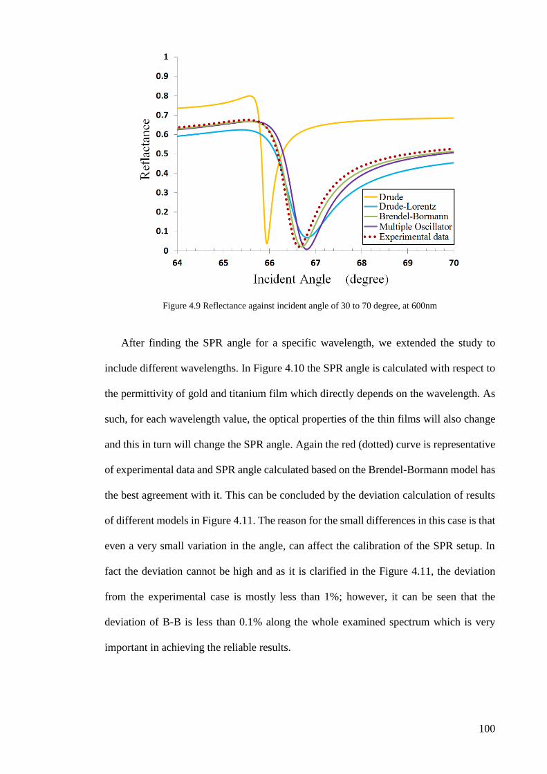
100
Figure 4.9 Reflectance against incident angle of 30 to 70 degree, at 600nm
After finding the SPR angle for a specific wavelength, we extended the study to
include different wavelengths. In Figure 4.10 the SPR angle is calculated with respect to
the permittivity of gold and titanium film which directly depends on the wavelength. As
such, for each wavelength value, the optical properties of the thin films will also change
and this in turn will change the SPR angle. Again the red (dotted) curve is representative
of experimental data and SPR angle calculated based on the Brendel-Bormann model has
the best agreement with it. This can be concluded by the deviation calculation of results
of different models in Figure 4.11. The reason for the small differences in this case is that
even a very small variation in the angle, can affect the calibration of the SPR setup. In
fact the deviation cannot be high and as it is clarified in the Figure 4.11, the deviation
from the experimental case is mostly less than 1%; however, it can be seen that the
deviation of B-B is less than 0.1% along the whole examined spectrum which is very
important in achieving the reliable results.
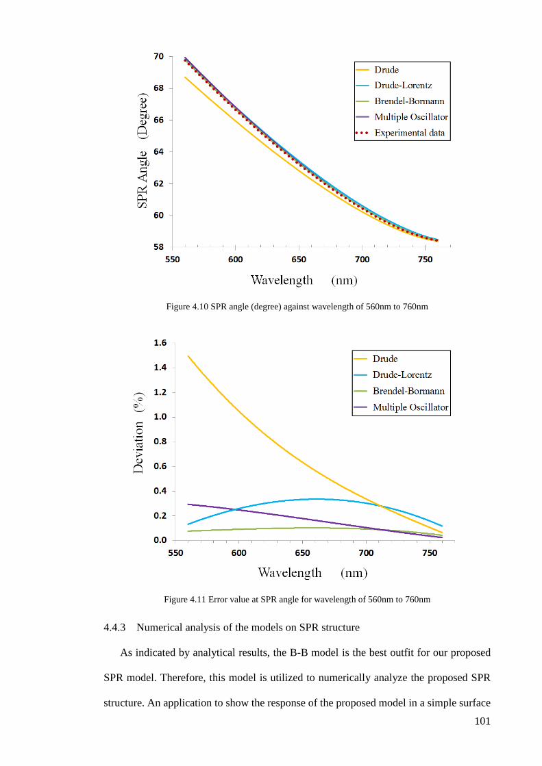
101
Figure 4.10 SPR angle (degree) against wavelength of 560nm to 760nm
Figure 4.11 Error value at SPR angle for wavelength of 560nm to 760nm
4.4.3 Numerical analysis of the models on SPR structure
As indicated by analytical results, the B-B model is the best outfit for our proposed
SPR model. Therefore, this model is utilized to numerically analyze the proposed SPR
structure. An application to show the response of the proposed model in a simple surface

102
plasmon structure is finding the power-flow in the cross-section of different layers. The
power-flow (also known as load-flow) is an important tool involving numerical analysis
that can be applied to a system. It is a factor related to propagation of the medium and for
surface analysis it can give us a good perspective for surface sensitivity.
Figure 4.12 shows the power flow of the SPR structure which is plotted versus time
average. In this figure the horizontal axis is shown the length of layer in the cross-section
of SPR structure. As it is obvious in this picture, the gradual increase in the power-flow
results in a sudden drop when passing from dielectric to metal (titanium on the left and
gold on the right side) while a small spike can be recognizing in the titanium and gold
boundary. It means that the surface is more sensitive when there is a dielectric-metal
boundary than metal-metal boundary. Also as much as the increase of the power flow at
near of the metal surface is sharper, the sensation is more related to that surface and if it
was broad, it can be interpreted as having a good spatial sensitivity. In the case as it is
clear the increase of the continuum is sharp and especially near the gold wall the
sensitivity is too high. Through Figure 4.12, we can observe that the simulated power-
flow using B-B model to calculate the optical properties of the layers (green curve at the
background) is well coincided with the simulated power-flow using experimental optical
properties (red dotted line).
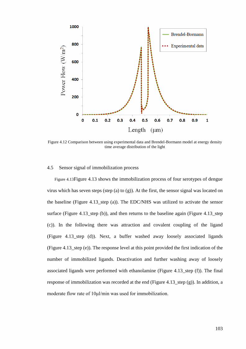
103
Figure 4.12 Comparison between using experimental data and Brendel-Bormann model at energy density
time average distribution of the light
4.5 Sensor signal of immobilization process
Figure 4.13Figure 4.13 shows the immobilization process of four serotypes of dengue
virus which has seven steps (step (a) to (g)). At the first, the sensor signal was located on
the baseline (Figure 4.13_step (a)). The EDC/NHS was utilized to activate the sensor
surface (Figure 4.13_step (b)), and then returns to the baseline again (Figure 4.13_step
(c)). In the following there was attraction and covalent coupling of the ligand
(Figure 4.13_step (d)). Next, a buffer washed away loosely associated ligands
(Figure 4.13_step (e)). The response level at this point provided the first indication of the
number of immobilized ligands. Deactivation and further washing away of loosely
associated ligands were performed with ethanolamine (Figure 4.13_step (f)). The final
response of immobilization was recorded at the end (Figure 4.13_step (g)). In addition, a
moderate flow rate of 10μl/min was used for immobilization.

104
Figure 4.13 Immobilization sensorgram of four serotypes of dengue antigen on sensor surface
4.6 Microscopic information of chip sensor
The SEM and AFM images support the virus immobilization has been done properly
in the following.
Figure 4.14 Imaging of the immobilization process on the gold surface using SEM

105
The surface on which the antigens (Ag) were immobilized was characterized using
scanning electron microscopy (FE/SEM Quanta FEG250) and atomic force microscopy
(VEECO DIMENSION 3000 AFM). AFM imaging was performed in contact mode using
0.01-0.025 Ohm-cm antimony (n)-doped silicon probes. Figure 4.14 exemplifies a typical
cross-sectional view of gold coating on glass accompanied by nanoparticles such as
amine groups and immobilized antigens. According to the SEM, the gold coating was
around 52nm thick.
Figure 4.15 displays the top view of the gold surface with immobilized antigens on
it. For further investigation 2D and 3D images of AFM were employed to prove the
existence of immobilized antigens (Figure 4.16 and Figure 4.17). The 3D AFM image
shows the surface of the gold-coated glass with two distinctive types of hills: first,
homogenous, dense and low gold hills resulting from amine groups and second, sporadic
higher hills created by immobilized antigens. The amine groups acted as a binding protein
to the sensing antigen, which anchored very well to the sensor surface.
Figure 4.15 Imaging of the immobilization process on the gold surface using SEM machine-
SEM top view of immobilized antigen surface

106
Figure 4.16 Two dimensional AFM image dengue antigen-dextran conjugate onto surface
Figure 4.17 Three dimensional AFM image dengue antigen-dextran conjugate onto surface

107
4.7 Determination of sample concentration
In this section, quantitative analysis is done to find out an optimized concentration of
the analyte which is in the fluid sample. For this study, the different concentrations of the
analyte are prepared and then applied in the separate analysis cycles for studying the SPR
sensor signal. The measured responses (sensorgrams) are presented in the separate plots
of Figure 4.18 with similar scale at different concentrations. The association phase of
sensorgram is reduced by decreasing analyte concentration. As the concentration of
analyte in the sample increases, the rising edge of produced response signal becomes
sharper. Hence, the optimum concentration is needed to be determined in order to avoid
rapid saturation of sensor signal and to have an appropriate regeneration as well.
All concentration tests are carried out in same conditions and used constant buffers.
The patient’s serum, which is diluted in sodium acetate with different concentrations for
each experiment, is injected on the sensor surface. Basically the free antibodies which are
on the sample bound to dengue antigens (already immobilized on the sensor surface)
produce a change in quantity of binding Ag-Ab interaction.
As mentioned, the response sensorgram shows the quantity of binding interaction on
the gold surface of the biosensor. With starting the injection of patient’s serum, we are
expecting that the response has an upward trend in the baseline level and represents the
amount of dengue antibodies bound during injection with its antigens.

108
Figure 4.18 Sensorgrams illustrate the evolution of resonance units (RU) versus time during association
and dissociation measurements along with biosensor regeneration performed in the Biacore instrument.
The inset schematics represent dengue antibodies (Y shapes) versus dengue antigens (immobilized circles
on surface)
Upon sensor surface construction, the experiments were conducted by exposing the
surface to each concentrated serum containing IgM antibody. The dengue IgM antibody
began to bind once the serum was introduced to the sensor surface; a process that
continued while an equilibrium position took place between the serum antibody
concentration and immobilized dengue antigen concentration. At this point, the process
of binding was studied by replacing the liquid phase with a buffer and recording the
dissociation of attached antibodies until an equilibrium ratio between dengue IgM

109
antibodies and immobilized antigens was achieved. These basic phases of association and
dissociation can be performed at different serum concentrations to examine the effect
concentration has on the time-dependent diagnostic process for the dengue virus
(Figure 4.18).
Two dips at the end of each sensorgram were anticipated (Figure 4.18) and based on
the Biacore setup. They indicate that the chip surface regenerated twice at the end of the
process and all Ag-Ab binding was washed out by the glycine buffer. Thereafter, the
sensor was ready for the subsequent experiments. The sensor surface was expected to be
sufficiently clear for the next binding with minimal influence from prior detection.
Evaluating the kinetic and equilibrium situations’ concentration dependence leads to
sample volume optimization under this study’s particular conditions. This experiment
was repeated under the same conditions, whereby all environmental variables (e.g.
temperature and buffers) were fixed to examine the effect of sample concentration. The
serum was diluted to concentrations of 1:25, 1:50, 1:100, 1:200, 1:400 and 1:800 by
adding 10mM sodium acetate solvent with pH 4.5.
In the study of serum concentration generally described in Figure 4.18, a high quantity
of dengue antibodies at a 1:25 concentration caused sudden, rapid saturation in the
binding phase between antibodies and antigens at the chip surface (Figure 4.18 (a)). Upon
saturation, the sensor’s accuracy decreased - meaning that virus recognition in the
detection procedure was not reliable.
However, the large quantity of antibodies rendered the washing phase difficult owing
to the lengthy duration of washing. The importance of the washing phase is more
prominent if the chip is used for the following assay. In Figure 4.18, the subplots (a) and
(b) show that chip regeneration did not occur adequately. The incomplete regeneration
indicates there remained a little Ag-Ab bound onto the chip surface in spite of

110
regeneration having been done twice. The subsequent incoming antibodies (suspended in
the next sample) would get bound to the free, immobilized antigens on the surface and
combined with previously bound antibody residue. Hence, both concentrations are
considered Ag-Ab binding in the next generated signal. The error caused by this chip
malfunction affects the entire diagnosis process. With a declining number of antibodies
by diluting the serum, their binding to the relevant immobilized antigens caused an
exponential bend in the sensorgram. The maximum saturation was still achievable by
diluting the serum to 1:100 (Figure 4.18 (c)). At concentrations of 1:200 (Figure 4.18
(d)), 1:400 (Figure 4.18 (e)), and 1:800 (Figure 4.18 (f)), the results signify that the
antibodies inside the serums did not attach to the immobilized antigens within the binding
timeframe. Consequently, binding in the serum diluted to 1:800 was nearly ineffective
(Figure 4.18 (f)). This happened because the low quantity of antibodies in the last sample
did not interact enough with the antigens on the surface.
These descriptions indicate the importance of accurate sample concentration. As
noted above, the concentration of 1:100 may serve as reference to provide high resolution
results. This concentration value also facilitates great surface regeneration and can rely
on sample amount for dengue virus detection.
In Figure 4.19, the changing SPR angle and biosensor regeneration were assessed
according to the different concentrations. In this comparison, the concentrations of 1:25,
1:50 and 1:100 exhibit the highest percentages of SPR angle alteration, whereas sensor
regeneration improved gradually. Although the sensor surface regeneration enhancement
is acceptable at more diluted concentrations (1:200, 1:400, and 1:800), the modifications
in SPR angle decrease and nearly vanish at 1:800, as explained in the final part. In view
of SPR angle variation and regeneration of biosensor parameters, the concentration of
1:100 is practically the best option for dengue virus detection with high sensitivity and
optimal chip regeneration.

111
Figure 4.19 (Blue) The stacked column graph represents the quantity of Ag-Ab bound on the sensor
surface, which is directly related to the amount of sensor sensitivity; Red represents chip surface cleaning
related to the quality of sensor regeneration
4.8 Examination of samples
The binding response sensorgram which resulted from dengue high positive serum
(as an example) along with control experiment as a reference, shows the quantity of
binding interaction on the gold surface of the biosensor (Figure 4.20). Starting with the
injection of patient sample, the response increases exponentially, representing the amount
of dengue antibodies bound during injection with its antigens (Figure 4.20 (a)). There will
be no binding if the patient sample does not carry the dengue antibodies or is carrying
non-dengue antibodies. In this condition, the patient sample is a true negative.
In Figure 4.20 (b), there are two dips located at the end of the sensorgram caused by
SPR setup adjustment. The dips indicate that the chip surface is regenerated twice and
washed out all Ag-Ab binding (by the glycine buffer). It is expected that the gold surface
of the sensor to be cleaned with the least influence of previous binding that can be proved
by the control experiment. It should be noted that the whole assay was performed in only
ten minutes.

112
Figure 4.20 The binding response curve termed by sensorgram, (a) the binding process and (b) the
regeneration of biosensor surface
Figure 4.21 manifests the SPR angle variations in terms of patient serum. As can be
seen, the maximum SPR angle variations occur in high positive (HP), mid positive (MP),
and low positive (LP) anti-dengue viruses respectively. Each HPs, MPs, and LPs are the
average of ten samples of their types and each bar can also be a reference for diagnosis
of each dengue virus types. This method can determine the ratio of four serotypes of
dengue virus and by utilizing this ratio, specialists can easily and correctly decide whether
to place the patients in observation (hospitalize) or sent home. The SPR angle variations
in each serotype of dengue virus tend to have a linear slope. These linearity variations
can generate boundaries that are distinguished by HP, MP, and LP.
A comparative study was performed to validate the results that obtained by proposed
SPR technique with conventional ELISA method (as presented in Table 4.1). As it can
be seen NS1, positive/negative (P/N) ratio and IgM results of each patient serum are
displayed based on ELISA method. The first test to be run is NS1 whose positive result
indicates the presence of dengue virus in blood, however, to gain further validity, IgM

113
test, too, needs to be conducted. It is vital to do IgM test for final confirmation in samples
with negative NS1.
Figure 4.21 SPR angle variation via patient's serum- Dengue virus diagnosis graph

114
Table 4.1 Comparative data base of ELISA and proposed SPR biosensor in low, mid and high positive
patient samples of dengue virus
Type of
sample
(HI)
Patient
serum
ELISA results Biosensor results (SPR )
P/N
ratio NS1 IgM S.T. 1 S.T. 2 S.T. 3 S.T. 4
Lo
w p
osi
tiv
e
(An
tib
od
y t
itre
10-1
60)
AH01 2.48 - + 1.0110 0.7454 0.5808 0.5923
AH02 2.67 - + 1.0570 0.7186 0.5845 0.6344
AH03 2.59 + + 1.0688 0.7211 0.5785 0.6369
AH04 2.47 + + 1.0013 0.6498 0.5499 0.5957
AH05 2.81 + + 1.0102 0.6694 0.5162 0.5572
AH06 2.47 + + 1.0060 0.6560 0.5080 0.5467
AH07 2.79 + + 0.9665 0.6910 0.5548 0.6105
AH08 2.14 + + 1.0019 0.7015 0.5002 0.5844
AH09 2.93 - + 1.1015 0.7528 0.5775 0.6512
AH10 2.58 - + 1.0104 0.7501 0.5771 0.6081
Mid
posi
tive
(An
tib
od
y t
itre
160-6
40)
AH11 3.01 + + 0.9983 0.8863 0.6866 0.7051
AH12 3.93 + + 1.0574 0.9095 0.5849 0.8077
AH13 3.45 - + 1.1691 0.7965 0.5987 0.7498
AH14 3.75 + + 0.9862 0.9380 0.6720 0.7899
AH15 3.34 - + 1.1001 0.8754 0.6972 0.7386
AH16 4.59 - + 1.1124 0.9566 0.7399 0.8211
AH17 4.5 + + 1.1092 0.9487 0.7410 0.8222
AH18 4.96 + + 1.1978 0.9637 0.7405 0.8230
AH19 4.34 - + 1.0543 0.7688 0.7337 0.6968
AH20 4.63 + + 1.1733 0.9598 0.7234 0.8176
Hig
h p
osi
tiv
e
(An
tib
od
y t
itre
12
80
-102
40
)
AH21 5.25 + + 1.1255 1.0114 0.7154 0.9045
AH22 5.69 + + 1.1469 0.9778 0.7740 0.8304
AH23 5.12 + + 1.1344 0.9463 0.7595 0.7983
AH24 5.6 + + 1.1226 0.9462 0.7519 0.8084
AH25 6.53 - + 1.1215 0.9084 0.7585 0.7845
AH26 7.13 - + 1.1987 1.0695 0.7021 0.8793
AH27 7.32 + + 1.2731 1.1128 0.8676 0.9519
AH28 6.06 + + 1.1996 0.9954 0.7567 0.8922
AH29 7.02 - + 1.2453 1.0532 0.8063 0.9476
AH30 7.38 - + 1.2782 0.9869 0.7631 0.8541

115
Table 4.1 contains the positive IgM results proving the presence of dengue virus in
all samples through IgM antibody quantity (P/N ratio). The results from the proposed
method show the binding ratio between IgM antibody in samples with all four serotypes
of the immobilized dengue virus on the chip surface. The changes in the bound antibody
quantity to surface in four serotypes were measured by monitoring the surface plasmon
resonance angle of each sample.
To know the sensitivity of detection by the sensor, the change of the angle matching
the minimum reflection coefficient called SPR angle ( .SPR ) was calculated for each
experiment (Table 4.1). Then the sensitivity of the sensor relates to the test's ability to
identify positive results compared with the results of conventional method, which is 83-
93% in this research.
The samples with TBE and HC viruses (negative dengue NS1 and subsequently
negative dengue IgM results) are presented in Table 4.2. The final outcome of the
proposed method indicates that there is an insignificant change in the SPR angle of all
four serotypes. Such a small change signals that there is no binding between TBE or HC
antibody that exists in samples and the serotypes of dengue virus. According to the
Table 4.2, there is no any false positive result, which has overlap with positive range of
each serotype. However, the specificity of the biosensor which is 100%, was calculated
by examining the sera from this table.

116
Table 4.2 The negative controls and the number of the serum samples were examined for the specificity
evaluation in this study.
Type of
sample
Patient
serum
ELISA results Biosensor results (|SPR |)
NS1 IgM S.T. 1 S.T. 2 S.T. 3 S.T. 4 T
ick
-Born
e E
nce
ph
ali
tis
SAM01 - - 0.31852 0.3760 0.19469 0.32879
SAM02 - - 0.15085 0.2557 0.21550 0.19386
SAM 03 - - 0.37746 0.2860 0.00040 0.19946
SAM 04 - - 0.16855 0.2940 0.04890 0.16955
SAM 05 - - 0.14738 0.1254 0.02943 0.13294
SAM 06 - - 0.02807 0.1651 0.25771 0.08001
SAM 07 - - 0.25098 0.0770 0.18170 0.10140
SAM 08 - - 0.03523 0.0973 0.02780 0.07478
SAM 09 - - 0.04094 0.0646 0.07810 0.04010
SAM 10 - - 0.05042 0.0050 0.01400 0.01260
SAM 11 - - 0.24308 0.0911 0.25786 0.04538
SAM 12 - - 0.11004 0.0011 0.25924 0.09303
SAM 13 - - 0.25980 0.1937 0.21978 0.09314
SAM 14 - - 0.35171 0.2944 0.31243 0.20877
SAM 15 - - 0.2852 0.1905 0.23039 0.10882
SAM 16 - - 0.21199 0.1115 0.14507 0.01650
SAM 17 - - 0.22769 0.1312 0.17126 0.03061
SAM 18 - - 0.28431 0.1407 0.15434 0.00509
SAM 19 - - 0.25883 0.1396 0.17210 0.04012
Hep
ati
tis
C
SAM 20 - - 0.21092 0.1737 0.23510 0.11329
SAM 21 - - 0.23587 0.1497 0.24237 0.09972
SAM 22 - - 0.30437 0.1798 0.19558 0.06360

117
4.9 Validating simulation based on experimental results
In this section, the experimental results compare with theoretical results from
mathematical analysis. According to the previous section, the change in SPR angle was
measured for rapid detection of anti-dengue virus in human serum samples
experimentally. Based on the relationship of SPR angle and refractive index, the
refractive index changes of binding medium for different serums can be acquired. In order
to show the accuracy of theoretical analysis, the obtained refractive index of samples are
applied to the proposed SPR configuration which has been presented in the methodology
section. Since there are a large number of samples, only one sample from each category
of dengue serotypes 2 (low, mid, and high positive) is selected and examined for
verification of the analytical analysis. With respect to the samples table (Table 4.1), the
SPR angle variation of sample AH 7, AH 12 and AH 29, which are as representative of
low, mid, and high positive dengue serotype 2 respectively, is presented along with their
refractive index changes in Figure 4.22.
Figure 4.22 Patients’ serum via SPR angle variation, and their refractive index changes

118
Based on samples table, the SPR angle variations were obtained 0.6910°, 0.9095°,
and 1.0532° for low, mid, and high positive patients’ serums with changing refractive
index 0.00691, 0.009095, and 0.01053 respectively.
Based on analytical investigation, the plot of totally reflected intensity versus angle
of incidence termed SPR curve was shown in left side of Figure 4.23. To generate a SPR
curve, we used a generalized 4-layer model (N = 4). The first layer is prism with refractive
index n1= nprism. The kth layer (k: 2 to N-1) has a thickness of dk and the local dielectric
function εk(λ0) or the refractive index nk(λ0). In λ0 = 633 nm, there are the prism (n1=
1.457) | gold (d2= 50 nm, n2= 0.2 + i3.32) | linker (d3= 100 nm, n3= 1.515) | binding
medium, where n4 was found from experimental results.
Figure 4.23 shows the SPR angle variations based on the mathematical model of SPR
structure. As discussed in Chapter 3, the obtained experimental changes in refractive
index for each samples were applied in the analytical model. These changes have been
schematically illustrated with corresponding sensorgrams in right side of Figure 4.23. The
SPR angle variations in low (A), mid (B), and high (C) positive dengue patient serums
were calculated 0.654°, 0.85°, and 1.014° respectively.
Table 4.3 shows the mathematical error for dengue detection in low, mid, and high
positive patients’ serums. According to this table, by experimental investigation on
analyte-ligand binding quantity and then analytical analysis of the biosensor based
practical conditions, we found the error ratio of each category (~5.35%, 6.54%, and
3.72%) compared to experimental results.
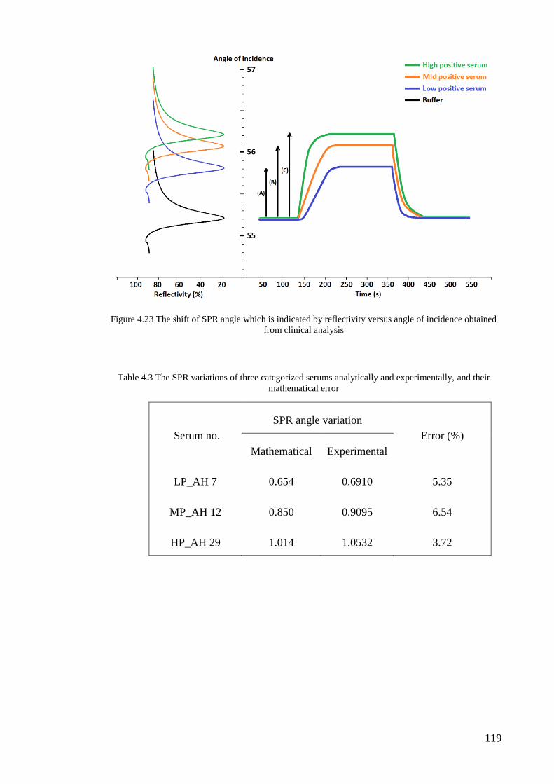
119
Figure 4.23 The shift of SPR angle which is indicated by reflectivity versus angle of incidence obtained
from clinical analysis
Table 4.3 The SPR variations of three categorized serums analytically and experimentally, and their
mathematical error
Serum no.
SPR angle variation
Error (%)
Mathematical Experimental
LP_AH 7 0.654 0.6910 5.35
MP_AH 12 0.850 0.9095 6.54
HP_AH 29 1.014 1.0532 3.72

120
5 CHAPTER V: CONCLUSION AND FUTURE WORK
The aim of the work in this thesis was to develop a technique for dengue rapid
diagnostic test. The development of this technique was successfully achieved by
employing the SPR method as an optical biosensor.
In this thesis, we applied Drude, Drude-Lorentz, Brendel-Bormann, and Multiple
Oscillator models to determine the most compatible and reliable model for SPR sensing
studies analytically and numerically. The main focus was on the SPR angle in different
wavelengths and also its reflectance in a specific wavelength. The mathematical results
revealed that Brendel-Bormann model generated the most accurate real and imaginary
permittivity values for the materials used in the proposed SPR structure, within the
wavelengths of interest. Moreover the Brendel-Bormann model results was more stable
and close to the experimental data as compared to the other models. The final numerical
analysis has been performed by simulating the power-flow of the SPR structure. The
numerical results supported mathematical work and proved that Brendel-Bormann model
can be trustable as its continuum is perfectly matched with the experimental data
calculated power-flow.
The value of the optimizing sample concentrations were determined by careful
examination of the different concentrations of sample, this is one of the main
contributions of this study. In order to obtain the well-regeneration of biochip, the sample
volume was optimized to the minimum amount of 1 µl of serum while maintaining high
sensitivity.
We then showed that the proposed SPR based biosensor is satisfactory for direct
determination of dengue Ag-Ab binding interaction on the sensor surface. Experimental
and computational investigations have been carried out in order to determine the dengue
Ag-Ab interactions occurring on the surface of the SPR biosensor. This study indicated

121
that the shifting of SPR angle in experimental and analytical results conform to each
other. The magnetic fields of the sensor surface were numerically simulated to show the
effect of different binding mediums. The SPR technique, despite of the conventional
methods, provides a rapid detection of dengue Ag-Ab interaction (i.e. around 10 minutes).
To investigate the four serotypes of dengue virus, the antigens of each serotype were
immobilized on the chip surface. A number of patient serums (categorized to the low,
mid, and high positive anti-dengue viruses) were passed onto the immobilized ligand.
The results showed that using the proposed method, the anti-dengue virus IgM in human
serum can be detected with high sensitivity and specificity responses.
According to the findings of this study, a specific portable device could be designed
and fabricated for rapid diagnostic tests of dengue fever in medical centers.
The presented work can be used to investigate several areas in the future. In the
sensing applications, this early detection technique can also be expanded to include an
identification of specific antibodies of other diseases such as Japanese encephalitis (JE)
and yellow fever.

122
APPENDIX A: Derivation dispersion relation; SP’s on planar surface
With Hz given by
1. A �⃗⃗� 𝑧 = 𝐴 ∙ exp{𝑗(𝜔𝑡 − 𝑞𝑥𝑥)} ∙ exp(𝛼𝑚𝑦) ∙ �⃗� 𝑦 (𝑦 < 0,𝑚𝑒𝑡𝑎𝑙)
2. A �⃗⃗� 𝑧 = 𝐵 ∙ exp{𝑗(𝜔𝑡 − 𝑞𝑥𝑥)} ∙ exp(−𝛼𝑑𝑦) ∙ �⃗� 𝑦 (𝑦 > 0, 𝑑𝑖𝑒𝑙𝑒𝑐𝑡𝑟𝑖𝑐)
and the Helmholtz wave equation
3. A ∇2𝐻𝑧 = −𝜔𝜇0휀0휀𝑟𝐻𝑧0
the reciprocal penetration depths 𝛼𝑚 and 𝛼𝑑 are obtained by substituting and Equation
A.2 into Equation A.3:
4. A 𝛼𝑚 = √𝑞𝑥2 − 𝑘02휀𝑚
5. A 𝛼𝑑 = √𝑞𝑥2 − 𝑘02휀𝑑
With Maxwell’s Equation A.4
6. A ∇ × �⃗⃗� = |
�⃗� 𝑥 �⃗� 𝑦 �⃗� 𝑧𝜕𝑥 𝜕𝑦 𝜕𝑧0 0 𝐻𝑧
| = 𝑖𝜔휀0휀𝑟�⃗�
and the boundary condition for the tangential components of E at y = 0 yields
7. A 1
𝜀0𝜀𝑚𝜕𝑦𝐻𝑧 =
1
𝜀0𝜀𝑑𝜕𝑦𝐻𝑧
where ∂x = ∂/∂x, likewise for y and z. Substituting Equation A.1 and Equation A.2 into
Equation A.7 yields 2.37. The same method can be used to verify that TE-plasmons
cannot exist on a flat metal surface. To this end, Ez is given in the same form as Hz for
TM-plasmons:
8. A �⃗� 𝑧 = 𝐴 ∙ exp{𝑗(𝜔𝑡 − 𝑞𝑥𝑥)} ∙ exp(𝛼𝑚𝑦) ∙ �⃗� 𝑦 (𝑦 < 0,𝑚𝑒𝑡𝑎𝑙)
9. A �⃗� 𝑧 = 𝐵 ∙ exp{𝑗(𝜔𝑡 − 𝑞𝑥𝑥)} ∙ exp(−𝛼𝑑𝑦) ∙ �⃗� 𝑦 (𝑦 > 0, 𝑑𝑖𝑒𝑙𝑒𝑐𝑡𝑟𝑖𝑐)

123
with 𝛼𝑚 and 𝛼𝑑 given by Equation A.4 and Equation A.5. With Maxwell’s 2.3 and the
boundary condition that the tangential component of H is continuous across the interface,
one obtains
11. A ∇ × �⃗� = |
�⃗� 𝑥 �⃗� 𝑦 �⃗� 𝑧𝜕𝑥 𝜕𝑦 𝜕𝑧0 0 𝐻𝑧
| = −𝑖𝜔𝜇0𝜇𝑟�⃗⃗�
11. A 1
𝜇𝑚𝜕𝑦𝐸𝑧 =
1
𝜇𝑑𝜕𝑦𝐸𝑧
12. A −𝛼𝑚
𝜇𝑚=𝛼𝑑
𝜇𝑑
In order to satisfy Equation A.12 either 𝜇𝑚 or 𝜇𝑑 has to be negative. However, the
relative permeability 𝜇𝑟 is constant and almost unity (or more precisely 𝜇𝑟 > 0) for all
metals at optical frequencies; hence no TE-plasmons can be excited.

124
APPENDIX B: Investigation of chip surface
There is a wide range of analytical techniques which can be used for characterization
of materials based on the type of information required from surface structure down to
nanometer scale. For surface investigation with high resolution, the two typically used
techniques are atomic force and scanning electron microscopies.
Since the ligands (dengue antigens) were immobilized onto the gold thin film, the
sensor chip (Figure B. 1); whether the properties of the layers and microscopic images of
highest layer; will be investigated using AFM and SEM machines. In the following the
required instruments will be introduced and accordingly discussed on their results in
results and discussions section.
Figure B. 1 The separated portion of sensor chip for studying its structure
I. Atomic force microscopy image
The atomic force microscopy (AFM) consists a scan of a sharp tip at the end of a
flexible cantilever onto a sample surface with a small constant force. The tip-sample
interactions are monitored to reflect a laser off the rear of the cantilever in the split
photodiode detector. By determining the difference of photo-detector output voltages, the
cantilever deflection changes and subsequently oscillation amplitude are specified.

125
The site of antigen (Ag) immobilization was characterized using atomic force
microscopy (VEECO DIMENSION 3000 AFM; Figure B. 2). AFM imaging was
performed in contact mode using 0.01-0.025 Ohm-cm antimony with the integrated
silicon tip and its cantilever. The 2D and 3D AFM images help to prove the existence of
immobilized antigens.
Figure B. 2 The atomic force microscopy instrument- Department of Physics, UM
II. Scanning electron microscope image
The operation of the scanning electron microscopy (SEM) consists an applied voltage
between the conductive pattern and filament, which results at electron emission from the
filament to the pattern (as a sample). It happens at a range of vacuum environment from
10-4 to 10-10 Torr. The electrons are conducted to the sample by an electromagnetic lenses
series in the column of electrons. The scanning electron microscopy (FE/SEM-FEG)
focused ion beam technique (model Quanta FEG250; Figure B. 3), is used for our
investigation.
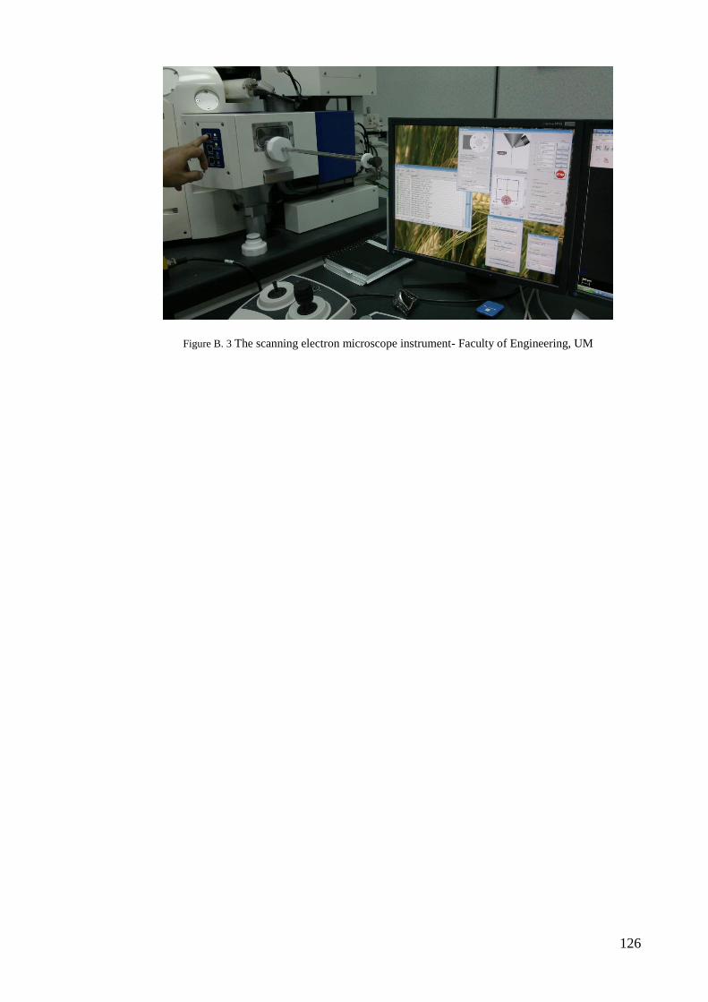
126
Figure B. 3 The scanning electron microscope instrument- Faculty of Engineering, UM
127
APPENDIX C: List of Publications, patent and innovation
Journal papers
Peyman Jahanshahi, Erfan Zalnezhad, Shamala Devi Sekaran & Faisal Rafiq
Mahamd Adikan; “Rapid Immunoglobulin M-Based Dengue Diagnostic Test
Using Surface Plasmon Resonance Biosensor”, Nature Scientific Reports,
2014.
Peyman Jahanshahi, Mostafa Ghomeishi, and Faisal Rafiq Mahamd Adikan;
“Study on Dielectric Function Models for Surface Plasmon Resonance
Structure”, Scientific World Journal, 2014.
Peyman Jahanshahi, Shamala Devi Sekaran, and Faisal Rafiq Mahamd Adikan;
“Optical and Analytical Investigations on Dengue Virus Rapid Diagnostic
Test for IgM Antibodies Detection”, Medical & Biological Engineering &
Computing, Minor Revision.
Peyman Jahanshahi, Mostafa Ghomeishi, Shamala Devi Sekaran & Faisal
Rafiq Mahamd Adikan; “Kinetic Analysis of IgM Monoclonal Antibodies for
Determination of Dengue Sample Concentration Using SPR Technique”,
Biomedical Optics Express, Under Revision.
Proceeding/Conference papers
Peyman Jahanshahi, Elian Dermosesian, and Faisal Rafiq Mahamd Adikan;
“Numerical and analytical investigation of a SPR structure as Biosensor”,
Frontiers in Optics (FiO) Conference, 19-23th October 2014, USA.
Peyman Jahanshahi, Barmak Honarvar Shakibaei, Shee Yu Gang and Faisal
Rafiq Mahamd Adikan; “Numerical Analysis of SPR-Based Optical Fiber
Biosensor”, 5th International Conference on Photonics 2014 (ICP2014),
2014, Malaysia.
128
Peyman Jahanshahi and Faisal Rafiq Mahamd Adikan; “Sensitivity
Enhancement of Graphene-Based Surface Plasmon Resonance Biosensor
Using Germanium Nanowires Grating“, Journal of Medical and
Bioengineering (JOMB), 2014, Australia.
Peyman Jahanshahi, Amin Parvizi, Faisal Rafiq Mahamd Adikan; “Three-
dimensional modeling of surface plasmon resonance based biosensor”,
Proc. SPIE 8801, Novel Biophotonic Techniques and Applications II, 2013,
Germany.
Peyman Jahanshahi, Hamid Toloue A.T, Anthony Ceteno, and Faisal Rafiq
Mahamd Adikan; “Numerical Analysis of Surface Plasmon Resonance
Biosensor Based on Graphene Layer”, The 8th AOTULE Deans Meeting,
Administrative Staff Meeting and Postgraduate Conference, 2013, Thailand.
Peyman Jahanshahi, Mostafa Ghomeishi, and Faisal Rafiq Mahamd Adikan;
“Adhesive Layer Effect on Gold-Silica Thin Film Interfaces for Surface
Plasmon Resonance Modeling”, 3rd International Conference on Photonics,
2012, Malaysia.
Patent and Innovation
NEW TECHNIQUE TO DIAGNOSE THE DENGUE VIRUS, Patent no.:
PI2014702566, 2014.
Name of Principal Investigator/ Inventor: Faisal Rafiq Mahamd
Adikan
Position: Professor
Faculty/Department: Electrical Engineering
Name of Co-Investigator/Co-Inventor: Peyman Jahanshahi
Position: PhD. Candidate/Research Assistant
Faculty/Department: Engineering/Electrical Engineering
Name of Co-Investigator/Co-Inventor: Erfan Zal Nezhad
Position: Doctor
Faculty/Department: Engineering/Mechanical Engineering
Name of Co-Investigator/Co-Inventor: Shamala Devi Sekaran
Position: Professor
Faculty/Department: Medicine/Microbiology

129
5TH EXPOSITION ON ISLAMIC INNOVATION (i-Inova2014), Nilai
Indoor Stadium, Negeri Sembilan, Malaysia, be held on 31st October - 2nd
November 2014.
Name of Principal Investigator/ Inventor: Faisal Rafiq Mahamd
Adikan
Position: Professor
Faculty/Department: Electrical Engineering
Name of Co-Investigator/Co-Inventor: Peyman Jahanshahi
Position: PhD. Candidate/Research Assistant
Faculty/Department: Engineering/Electrical Engineering
Name of Co-Investigator/Co-Inventor: Erfan Zal Nezhad
Position: Doctor
Faculty/Department: Engineering/Mechanical Engineering
Name of Co-Investigator/Co-Inventor: Shamala Devi Sekaran
Position: Professor
Faculty/Department: Medicine/Microbiology

130
REFERENCES
Abarbanel, S., & Gottlieb, D. (1997). A Mathematical Analysis of the PML Method.
Journal of Computational Physics, 134(2), 357–363.
Abdelghani, A., Chovelon, J. M., Jaffrezic-Renault, N., Ronot-Trioli, C., Veillas, C., &
Gagnaire, H. (1997). Surface plasmon resonance fibre-optic sensor for gas detection.
Sensors and Actuators B: Chemical, 39(1), 407–410.
Abdulhalim, I., Zourob, M., & Lakhtakia, A. (2008). Surface plasmon resonance for
biosensing: a mini-review. Electromagnetics, 28(3), 214–242.
Ahmet Arca. (2010). The design and optimisation of nanophotonic devices using the
Finite Element Method. University of Nottingham.
Amotchkina, T. V, Trubetskov, M. K., Tikhonravov, A. V, Janicki, V., Sancho-Parramon,
J., & Zorc, H. (2011). Comparison of two techniques for reliable characterization of
thin metal-dielectric films. Applied Optics, 50(33), 6189–97.
Ashley, J. C., & Emerson, L. C. (1974). Dispersion relations for non-radiative surface
plasmons on cylinders. Surface Science, 41(2), 615–618.
Azzam, R. M. A., & Bashara, N. M. (1987). Ellipsometry and polarized light. North-
Holland. sole distributors for the USA and Canada, Elsevier Science Publishing Co.,
Inc.
Barnes, W. L., Dereux, A., & Ebbesen, T. W. (2003). Surface plasmon subwavelength
optics. Nature, 424(6950), 824–830.
Berini, P. (1999). Plasmon polariton modes guided by a metal film of finite width. Optics
Letters, 24(15), 1011–1013.
Berini, P. (2006). Figures of merit for surface plasmon waveguides. Optics Express,
14(26), 13030–42.
Berini, P. (2008). Bulk and surface sensitivities of surface plasmon waveguides. New
Journal of Physics, 10(10), 105010.
Berini, P. (2009). Long-range surface plasmon polaritons. Advances in Optics and
Photonics, 1(3), 484.
Bhatia, P., & Gupta, B. D. (2012). Sensors and Actuators B : Chemical Fabrication and
characterization of a surface plasmon resonance based fiber optic urea sensor for
biomedical applications. Sensors & Actuators: B. Chemical, 161(1), 434–438.
Bhatt, S., Gething, P. W., Brady, O. J., Messina, J. P., Farlow, A. W., Moyes, C. L., …
others. (2013). The global distribution and burden of dengue. Nature.
Bohm, D., & Pines, D. (1951). A collective description of electron interactions. I.
Magnetic interactions. Physical Review, 82(5), 625.

131
Bohm, D., & Pines, D. (1953). A collective description of electron interactions: III.
Coulomb interactions in a degenerate electron gas. Physical Review, 92(3), 609.
Boltovets, P. M., Snopok, B. a, Boyko, V. R., Shevchenko, T. P., Dyachenko, N. S., &
Shirshov, Y. M. (2004). Detection of plant viruses using a surface plasmon
resonance via complexing with specific antibodies. Journal of Virological Methods,
121(1), 101–6.
Bozhevolnyi, S. I. (2006). Effective-index modeling of channel plasmon polaritons.
Optics Express, 14(20), 9467–9476.
Brenner, S. C., & Scott, R. (2008). The mathematical theory of finite element methods
(Vol. 15). Springer.
Brongersma, M. L., & Kik, P. G. (2007). Surface plasmon nanophotonics (Vol. 131).
Springer Berlin.
Burke, J. J., Stegeman, G. I., & Tamir, T. (1986). Surface-polariton-like waves guided by
thin, lossy metal films. Physical Review B, 33(8), 5186.
Campbell, C. T., & Kim, G. (2007). SPR microscopy and its applications to high-
throughput analyses of biomolecular binding events and their kinetics. Biomaterials,
28(15), 2380–92.
Chadwick, B., & Gal, M. (1993). An optical temperature sensor using surface plasmons.
Japanese Journal of Applied Physics, 32(6A), 2716–2717.
Cheesbrough, M. (2006). District laboratory practice in tropical countries (Vol. 2).
Cambridge university press.
Chen, S.-J., Chien, F. C., Lin, G. Y., & Lee, K. C. (2004). Enhancement of the resolution
of surface plasmon resonance biosensors by control of the size and distribution of
nanoparticles. Optics Letters, 29(12), 1390–1392.
Chernozatonskii, L. A., Ermoshin, S. N., & Gramotnev, D. K. (1991). Coupled Gulyayev-
Bleustein waves in a system of two different piezoelectrics separated by a gap.
Physics Letters A, 154(9), 465–470.
Chhatre, A., Solasa, P., Sakle, S., Thaokar, R., & Mehra, A. (2012). Colloids and Surfaces
A : Physicochemical and Engineering Aspects Color and surface plasmon effects in
nanoparticle systems : Case of silver nanoparticles prepared by microemulsion
route. Colloids and Surfaces A: Physicochemical and Engineering Aspects, 404, 83–
92.
Chinowsky, T. M., Saban, S. B., & Yee, S. S. (1996). Experimental data from a trace
metal sensor combining surface plasmon resonance with anodic stripping
voltammetry. Sensors and Actuators B: Chemical, 35(1), 37–43.
Courant, R., & others. (1943). Variational methods for the solution of problems of
equilibrium and vibrations. Bull. Amer. Math. Soc, 49(1), 1–23.
Crowther, J. R. (2000). The ELISA guidebook (Vol. 149). Springer.

132
DaCosta, R. S., Wilson, B. C., & Marcon, N. E. (2005). Optical techniques for the
endoscopic detection of dysplastic colonic lesions. Current Opinion in
Gastroenterology, 21(1), 70–79.
Djurisic, A. B., Fritz, T., & Leo, K. (2000). Modelling the optical constants of organic
thin films: impact of the choice of objective function. Journal of Optics A: Pure and
Applied Optics, 2(5), 458.
Document_not_found. (n.d.). Document not found ((Sang, L. S. Hoon, a Cuzzubbo, et
al., 1998; Tricou et al., 2010)).
Dostálek, J., & Knoll, W. (2008). Biosensors based on surface plasmon-enhanced
fluorescence spectroscopy (Review). Biointerphases, 3(3), FD12–FD22.
Dragoman, M., & Dragoman, D. (2008). Plasmonics: Applications to nanoscale terahertz
and optical devices. Progress in Quantum Electronics, 32(1), 1–41.
Dussart, P., Petit, L., Labeau, B., Bremand, L., Leduc, A., Moua, D., … Baril, L. (2008).
Evaluation of two new commercial tests for the diagnosis of acute dengue virus
infection using NS1 antigen detection in human serum. PLoS Neglected Tropical
Diseases, 2(8), e280.
Dutra, N. R., de Paula, M. B., de Oliveira, M. D., de Oliveira, L. L., & De Paula, S. O.
(2009). The laboratorial diagnosis of dengue: applications and implications. Journal
of Global Infectious Diseases, 1(1), 38–44.
Duzgun, A., Schuntner, C. A., Wright, I. G., Leatch, G., & Waltisbuhl, D. J. (1988). A
sensitive ELISA technique for the diagnosis of< i> Anaplasma marginale</i>
infections. Veterinary Parasitology, 29(1), 1–7.
Economou, E. N. (1969). Surface plasmons in thin films. Physical Review, 182(2), 539.
Englebienne, P., Hoonacker, A. Van, & Verhas, M. (2003). Surface plasmon resonance:
principles, methods and applications in biomedical sciences. Spectroscopy, 17(2,3),
255–273.
Fano, U. (1941). The theory of anomalous diffraction gratings and of quasi-stationary
waves on metallic surfaces (Sommerfeld’s waves). JOSA, 31(3), 213–222.
Fatemeh, D., Reza, Z. M., Mohammad, A., Salomeh, K., Reza, A. G., Hossein, S., …
others. (2014). Rapid detection of coliforms in drinking water of Arak city using
multiplex PCR method in comparison with the standard method of culture (Most
Probably Number). Asian Pacific Journal of Tropical Biomedicine, 4(5), 404.
Fox, A. M. (2001). Optical properties of solids (Vol. 3). Oxford university press.
Fry, S. R., Meyer, M., Semple, M. G., Simmons, C. P., Sekaran, S. D., Huang, J. X., …
Cooper, M. a. (2011). The diagnostic sensitivity of dengue rapid test assays is
significantly enhanced by using a combined antigen and antibody testing approach.
PLoS Neglected Tropical Diseases, 5(6), e1199.

133
Garg, R. (2008). Analytical and computational methods in electromagnetics. Artech
house.
GE Healthcare. (2008). Biacore 3000 Instrument Handbook.
General Electric Company, Biacore. (2014).
Ghosh, G. (1998). Handbook of Optical Constants of Solids: Handbook of Thermo-Optic
Coefficients of Optical Materials with Applications. Academic Press.
Gibson, W. C. (2007). The method of moments in electromagnetics. CRC press.
Girard, C., & Dereux, A. (1996). Near-field optics theories. Reports on Progress in
Physics, 59(5), 657.
Goodrich, T. T., Lee, H. J., & Corn, R. M. (2004). Direct detection of genomic DNA by
enzymatically amplified SPR imaging measurements of RNA microarrays. Journal
of the American Chemical Society, 126(13), 4086–4087.
Gordon Ii, J. G., & Ernst, S. (1980). Surface plasmons as a probe of the electrochemical
interface. Surface Science, 101(1), 499–506.
Gramotnev, D. K. (2005). Adiabatic nanofocusing of plasmons by sharp metallic grooves:
Geometrical optics approach. Journal of Applied Physics, 98(10), 104302.
Gramotnev, D. K., & Vernon, K. C. (2007). Adiabatic nano-focusing of plasmons by
sharp metallic wedges. Applied Physics B, 86(1), 7–17.
Gubler, D. J., & Clark, G. G. (1995). Dengue/dengue hemorrhagic fever: the emergence
of a global health problem. Emerging Infectious Diseases, 1(2), 55.
Guzman, M. G., Jaenisch, T., Gaczkowski, R., Hang, V. T. T., Sekaran, S. D., Kroeger,
A., … others. (2010). Multi-country evaluation of the sensitivity and specificity of
two commercially-available NS1 ELISA assays for dengue diagnosis. PLoS
Neglected Tropical Diseases, 4(8), e811.
Hagness, S. C., & Taflove, A. (2000). Computational Electrodynamics: The Finite-
Difference Time-Domain Method (Artech House Antennas And Propagation
Library) A.
He, H., Yuan, Y., Wang, W., Chiou, N.-R., Epstein, A. J., & Lee, L. J. (2009). Design
and testing of a microfluidic biochip for cytokine enzyme-linked immunosorbent
assay. Biomicrofluidics, 3(2), 22401.
Hertel, P. (2011). The Drude Model Model, (November).
Hessel, A., & Oliner, A. A. (1965). A new theory of Wood’s anomalies on optical
gratings. Applied Optics, 4(10), 1275–1297.
Homola, J. (2003). Present and future of surface plasmon resonance biosensors.
Analytical and Bioanalytical Chemistry, 377(3), 528–539.

134
Homola, J. (2008). Surface plasmon resonance sensors for detection of chemical and
biological species. Chemical Reviews, 108(2), 462–93.
Homola, J., Dostalek, J., Chen, S., Rasooly, A., Jiang, S., & Yee, S. S. (2002). Spectral
surface plasmon resonance biosensor for detection of staphylococcal enterotoxin B
in milk. International Journal of Food Microbiology, 75(1), 61–69.
Homola, J. iˇrí. (2006a). Electromagnetic theory of surface plasmons. In Surface Plasmon
Resonance Based Sensors (pp. 3–44). Springer.
Homola, J. iˇrí. (2006b). Surface plasmon resonance based sensors (Vol. 4). Springer.
Homola, J., Yee, S. S., & Gauglitz, G. (1999). Surface plasmon resonance sensors:
review. Sensors and Actuators B: Chemical, 54(1–2), 3–15.
Honório, N. A., Nogueira, R. M. R., Codeço, C. T., Carvalho, M. S., Cruz, O. G.,
Magalhães, M. de A. F. M., … others. (2009). Spatial evaluation and modeling of
dengue seroprevalence and vector density in Rio de Janeiro, Brazil. PLoS Neglected
Tropical Diseases, 3(11), e545.
Huebner, K. H., Dewhirst, D. L., Smith, D. E., & Byrom, T. G. (2008). The finite element
method for engineers. John Wiley & Sons.
Hunsperger, E. a, Yoksan, S., Buchy, P., Nguyen, V. C., Sekaran, S. D., Enria, D. a, …
Peeling, R. W. (2009). Evaluation of commercially available anti-dengue virus
immunoglobulin M tests. Emerging Infectious Diseases, 15(3), 436–40.
Hutter, E., & Fendler, J. H. (2004). Exploitation of localized surface plasmon resonance.
Advanced Materials, 16(19), 1685–1706.
I. Nomadics, Sensiq website. (2014).
Initiative, P. D. V., & others. (2005). Dengue diagnostics: proceedings of a joint
TDR/WHO and PDVI workshop: 4-6 October 2004, Geneva, Switzerland.
J. A. C. Weideman. (1994). Computation of the Complex Error Function.
Jönsson, U., Fägerstam, L., Ivarsson, B., Johnsson, B., Karlsson, R., Lundh, K., …
Rönnberg, I. (1991). Real-time biospecific interaction analysis using surface
plasmon resonance and a sensor chip technology. Biotechniques, 11(5), 620–627.
Jung, C. C., Saban, S. B., Yee, S. S., & Darling, R. B. (1996). Chemical electrode surface
plasmon resonance sensor. Sensors and Actuators B: Chemical, 32(2), 143–147.
Kim, E., DeMarco, S. J., Marfatia, S. M., Chishti, A. H., Sheng, M., & Strehler, E. E.
(1998). Plasma membrane Ca2+ ATPase isoform 4b binds to membrane-associated
guanylate kinase (MAGUK) proteins via their PDZ (PSD-95/Dlg/ZO-1) domains.
Journal of Biological Chemistry, 273(3), 1591–1595.
Knoll, W. (1998). Interfaces and thin films as seen by bound electromagnetic waves.
Annual Review of Physical Chemistry, 49(1), 569–638.
135
Koubova, V., Brynda, E., Karasova, L., Škvor, J., Homola, J., Dostalek, J., … Rošick\`y,
J. (2001). Detection of foodborne pathogens using surface plasmon resonance
biosensors. Sensors and Actuators B: Chemical, 74(1), 100–105.
Kretschmann, E., & Raether, H. (1968). Radiative decay of non radiative surface
plasmons excited by light(Surface plasma waves excitation by light and decay into
photons applied to nonradiative modes). Zeitschrift Fuer Naturforschung, Teil A, 23,
2135.
Kumarasamy, V., Chua, S. K., Hassan, Z., Wahab, a H. a, Chem, Y. K., Mohamad, M.,
& Chua, K. B. (2007). Evaluating the sensitivity of a commercial dengue NS1
antigen-capture ELISA for early diagnosis of acute dengue virus infection.
Singapore Medical Journal, 48(7), 669–73.
Kumarasamy, V., Wahab, a H. A., Chua, S. K., Hassan, Z., Chem, Y. K., Mohamad, M.,
& Chua, K. B. (2007). Evaluation of a commercial dengue NS1 antigen-capture
ELISA for laboratory diagnosis of acute dengue virus infection. Journal of
Virological Methods, 140(1-2), 75–9.
Kumbhat, S., Sharma, K., Gehlot, R., Solanki, A., & Joshi, V. (2010). Surface plasmon
resonance based immunosensor for serological diagnosis of dengue virus infection.
Journal of Pharmaceutical and Biomedical Analysis, 52(2), 255–9.
Lazcka, O., Campo, F., & Munoz, F. X. (2007). Pathogen detection: a perspective of
traditional methods and biosensors. Biosensors and Bioelectronics, 22(7), 1205–
1217.
Lee, K. (2008). World Health Organisation. Routledge.
Liedberg, B., Nylander, C., & Lundström, I. (1995). Biosensing with surface plasmon
resonance—how it all started. Biosensors and Bioelectronics, 10(8), i–ix.
Liedberg, B., Nylander, C., & Lunström, I. (1983). Surface plasmon resonance for gas
detection and biosensing. Sensors and Actuators, 4(0), 299–304.
Lim, V. (2009). Occupational infections. Malaysian J Pathol, 31(1), 1–9.
Maier, S. A. (2007). Plasmonics: fundamentals and applications. Springer.
Margheri, G., D’Agostino, R., Becucci, L., Guidelli, R., Tiribilli, B., & Del Rosso, M.
(2012). Surface plasmon resonance as detection tool for lipids lateral mobility in
biomimetic membranes. Biomedical Optics Express, 3(12), 3119–3126.
Margheri, G., Mannoni, A., & Quercioli, F. (1997). High-resolution angular and
displacement sensing based on the excitation of surface plasma waves. Applied
Optics, 36(19), 4521–4525.
Martinos, S. S., & Economou, E. N. (1981). Excitation of surface plasmons in cylinders
by electrons. Physical Review B, 24, 6908–6914.
Martinos, S. S., & Economou, E. N. (1983). Virtual surface plasmons in cylinders.
Physical Review B, 28, 3173–3181.

136
Mathers, C. D., Fat, D. M., & Boerma, J. T. (2008). The global burden of disease: 2004
update. World Health Organization.
Mcdonnell, J. M. (2001). Surface plasmon resonance : towards an understanding of the,
572–577.
Meek, J. L. (1996). A brief history of the beginning of the finite element method.
International Journal for Numerical Methods in Engineering, 39, 3761–3774.
Mernagh, D. R., Janscak, P., Firman, K., & Kneale, G. G. (1998). Protein-Protein and
Protein-DNA Interactions in the Type I. Restriction Endonuclease R. EcoR124I.
Biological Chemistry, 379(4-5), 497–504.
Mizutani, U. (2001). Introduction to the electron theory of metals. Cambridge University
Press.
Mouvet, C., Harris, R. D., Maciag, C., Luff, B. J., Wilkinson, J. S., Piehler, J., … Ismail,
G. (1997). Determination of simazine in water samples by waveguide surface
plasmon resonance. Analytica Chimica Acta, 338(1), 109–117.
Murray, N. E. A., Quam, M. B., & Wilder-Smith, A. (2013). Epidemiology of dengue:
past, present and future prospects. Clinical Epidemiology, 5, 299.
Naimushin, A. N., Soelberg, S. D., Nguyen, D. K., Dunlap, L., Bartholomew, D., Elkind,
J., … Furlong, C. E. (2002). Detection of Staphylococcus aureus enterotoxin B at
femtomolar levels with a miniature integrated two-channel surface plasmon
resonance (SPR) sensor. Biosensors & Bioelectronics, 17(6-7), 573–84.
Newton, R. G. (1982). Scattering theory of waves and particles. DoverPublications. com.
Novotny, L., & Hecht, B. (2012). Principles of nano-optics. Cambridge university press.
Nunes, M. R. T., Nunes Neto, J. P., Casseb, S. M. M., Nunes, K. N. B., Martins, L. C.,
Rodrigues, S. G., … Vasconcelos, P. F. C. (2011). Evaluation of an immunoglobulin
M-specific capture enzyme-linked immunosorbent assay for rapid diagnosis of
dengue infection. Journal of Virological Methods, 171(1), 13–20.
Nylander, C., Liedberg, B., & Lind, T. (1983). Gas detection by means of surface plasmon
resonance. Sensors and Actuators, 3, 79–88.
Oliveira, L. C., Moreira, S., Thirstrup, C., Uwe, E., Melcher, K., Marcus, A., … Neff, H.
(2013). A Surface Plasmon Resonance Biochip Wavelength Interrogation Modes,
62(5), 1223–1232.
Ordal, M. A., Long, L. L., Bell, R. J., Bell, S. E., Bell, R. R., Alexander Jr, R. W., …
others. (1983). Optical properties of the metals al, co, cu, au, fe, pb, ni, pd, pt, ag, ti,
and w in the infrared and far infrared. Applied Optics, 22(7), 1099–1119.
Organization, W. H., & others. (2011). Comprehensive guidelines for prevention and
control of dengue and dengue haemorrhagic fever. WHO Regional Publication
SEARO, (29).

137
Osman, O., Fong, M. Y., & Devi, S. (2007). Short Communication A Preliminary Study
of Dengue Infection in Brunei, 60, 205–208.
Otto, A. (1968). Excitation of nonradiative surface plasma waves in silver by the method
of frustrated total reflection. Zeitschrift F{ü}r Physik, 216(4), 398–410.
Palik, E. D. (1998). Handbook of Optical Constants of Solids: Index (Vol. 3). Access
Online via Elsevier.
Peeling, R. W., Artsob, H., Pelegrino, J. L., Buchy, P., Cardosa, M. J., Devi, S., … others.
(2010). Evaluation of diagnostic tests: dengue. Nature Reviews Microbiology, 8,
S30–S37.
Pfeiffer, C. A., Economou, E. N., & Ngai, K. L. (1974). Surface polaritons in a circularly
cylindrical interface: surface plasmons. Physical Review B, 10(8), 3038.
Piliarik, M., Sípová, H., Kvasnička, P., Galler, N., Krenn, J. R., & Homola, J. (2012).
High-resolution biosensor based on localized surface plasmons. Optics Express,
20(1), 672–80.
Pines, D. (1953). A collective description of electron interactions: IV. Electron interaction
in metals. Physical Review, 92(3), 626.
Pines, D., & Bohm, D. (1952). A collective description of electron interactions: II.
Collective vs individual particle aspects of the interactions. Physical Review, 85(2),
338.
Pockrand, I., Swalen, J. D., Gordon II, J. G., & Philpott, M. R. (1978). Surface plasmon
spectroscopy of organic monolayer assemblies. Surface Science, 74(1), 237–244.
Powell, C. J., & Swan, J. B. (1959). Origin of the characteristic electron energy losses in
aluminum. Physical Review, 115(4), 869.
Powell, C. J., & Swan, J. B. (1960). Effect of oxidation on the characteristic loss spectra
of aluminum and magnesium. Physical Review, 118(3), 640.
Prade, B., Vinet, J. Y., & Mysyrowicz, A. (1991). Guided optical waves in planar
heterostructures with negative dielectric constant. Phys. Rev. B, 44(24), 13556–
13572.
Prasad, P. N. (2004). Nanophotonics. Wiley. com.
Qi, Z., Honma, I., & Zhou, H. (2006). Humidity sensor based on localized surface
plasmon resonance of multilayer thin films of gold nanoparticles linked with
myoglobin. Optics Letters, 31(12), 1854–1856.
Quail, J. C., & Simon, H. J. (1984). Second-harmonic generation with phase-matched
long-range and short-range surface plasmons. Journal of Applied Physics, 56(9),
2589–2591.
Raether, H. (1988a). Surface plasmons on gratings. Surface Plasmons on Smooth and
Rough Surfaces and on Gratings, 91–116.

138
Raether, H. (1988b). Surface plasmons on smooth surfaces. Springer.
Rakic, A. D., Djurisic, A. B., Elazar, J. M., & Majewski, M. L. (1998). Optical properties
of metallic films for vertical-cavity optoelectronic devices. Applied Optics, 37(22),
5271–83.
Ramirez, A. H., Moros, Z., Comach, G., Zambrano, J., Bravo, L., Pinto, B., … Liprandi,
F. (2009). Evaluation of dengue NS1 antigen detection tests with acute sera from
patients infected with dengue virus in Venezuela. Diagnostic Microbiology and
Infectious Disease, 65(3), 247–253.
Ranjit, S., & Kissoon, N. (2011). Dengue hemorrhagic fever and shock syndromes*.
Pediatric Critical Care Medicine, 12(1), 90–100.
Reichert, Inc. , Reichert Surface Plasmon Resonance (SPR) Systems. (2014).
Rigau-Pérez, J. G., Clark, G. G., Gubler, D. J., Reiter, P., Sanders, E. J., & Vance
Vorndam, A. (1998). Dengue and dengue haemorrhagic fever. The Lancet,
352(9132), 971–977.
Ritchie, R. H. (1957). Plasma losses by fast electrons in thin films. Physical Review,
106(5), 874.
Rosenauer, A. (2003). Transmission electron microscopy of semiconductor
nanostructures: an analysis of composition and strain state (Vol. 2403). Springer.
Ruiz, E. G., Garces, I., Aldea, C., Lopez, M. A., Mateo, J., Alonso-Chamarro, J., &
Alegret, S. (1993). Industrial process sensor based on surface plasmon resonance
(SPR) 1. Distillation process monitoring. Sensors and Actuators A: Physical, 37,
221–225.
Sabatino, L., Botto, N., Borghini, A., Turchi, S., & Andreassi, M. G. (2013).
Development of a new multiplex quantitative real-time PCR assay for the detection
of the mtDNA4977 deletion in coronary artery disease patients: A link with telomere
shortening. Environmental and Molecular Mutagenesis, 54(5), 299–307.
Sadiku, M. N. O. (2010). Numerical techniques in electromagnetics. CRC press.
Sang, C. T., Hoon, L. S., Cuzzubbo, a, & Devine, P. (1998). Clinical evaluation of a rapid
immunochromatographic test for the diagnosis of dengue virus infection. Clinical
and Diagnostic Laboratory Immunology, 5(3), 407–9.
Sang, C. T., Hoon, L. S., Cuzzubbo, A., & Devine, P. (1998). Clinical evaluation of a
rapid immunochromatographic test for the diagnosis of dengue virus infection.
Clinical and Diagnostic Laboratory Immunology, 5(3), 407–409.
Schaller, J. K., Czepluch, R., & Stojanoff, C. G. (1997). Plasmon spectroscopy for high
resolution angular measurements. In Proc. SPIE (Vol. 3098, pp. 476–486).
Schilling, S., Ludolfs, D., Van An, L., & Schmitz, H. (2004). Laboratory diagnosis of
primary and secondary dengue infection. Journal of Clinical Virology, 31(3), 179–
184.

139
Schmidt, A. G., Lee, K., Yang, P. L., & Harrison, S. C. (2012). Small-molecule inhibitors
of dengue-virus entry. PLoS Pathogens, 8(4), e1002627.
Schulz, L. G. (1954). The optical constants of silver, gold, copper, and aluminum. I. The
absorption coefficient k. JOSA, 44(5), 357–362.
Schulz, L. G., & Tangherlini, F. R. (1954). Optical constants of silver, gold, copper, and
aluminum. II. The index of refraction n. JOSA, 44(5), 362–367.
Seydack, M. (2005). Nanoparticle labels in immunosensing using optical detection
methods. Biosensors and Bioelectronics, 20(12), 2454–2469.
Shalabney, A., & Abdulhalim, I. (2012). Figure-of-merit enhancement of surface
plasmon resonance sensors in the spectral interrogation. Optics Letters, 37(7), 1175–
7.
Shalaev, V. M., & Kawata, S. (2006). Nanophotonics with surface plasmons. Elsevier.
Shamala, D. (2008). Dengue: Breakbone fever, hemorrhagia or shock. JUMMEC, 11(2),
39–52.
Shamala, D. S. (2005). DENGUE AND DENGUE HAEMORRHAGIC FEVER IN
MALAYSIA. JUMMEC JUMMEC, 11.
Sharma, A. K., Jha, R., & Gupta, B. D. (2007). Fiber-optic sensors based on surface
plasmon resonance: a comprehensive review. Sensors Journal, IEEE, 7(8), 1118–
1129.
Shu, P.-Y., Chen, L.-K., Chang, S.-F., Yueh, Y.-Y., Chow, L., Chien, L.-J., … Huang, J.-
H. (2003). Comparison of capture immunoglobulin M (IgM) and IgG enzyme-linked
immunosorbent assay (ELISA) and nonstructural protein NS1 serotype-specific IgG
ELISA for differentiation of primary and secondary dengue virus infections.
Clinical and Diagnostic Laboratory Immunology, 10(4), 622–630.
Shu, P.-Y., & Huang, J.-H. (2004). Current advances in dengue diagnosis. Clinical and
Diagnostic Laboratory Immunology, 11(4), 642–650.
Skullsinthestars. (2010). Optics basics: surface plasmons. Retrieved from
http://skullsinthestars.com/2010/09/21/optics-basics-surface-plasmons/
Slavík, R., & Homola. (2007). Ultrahigh resolution long range surface plasmon-based
sensor. Sensors and Actuators B: Chemical, 123(1), 10–12.
Sólyom, J. (2010). Fundamentals of the Physics of Solids: Volume 3-Normal, Broken-
Symmetry, and Correlated Systems (Vol. 3). Springer.
Sommerfeld, A. (1909). Propagation of waves in wireless telegraphy. Ann. Phys, 28(3),
665–736.
Special Programme for Research, Training in Tropical Diseases, W. H. O. (2009).
Dengue: guidelines for diagnosis, treatment, prevention and control. World Health
Organization.

140
Stenzel, O., Wilbrandt, S., Stendal, A., Beckers, U., Voigtsberger, K., & Von
Borczyskowski, C. (1995). The incorporation of metal clusters into thin organic dye
layers as a method for producing strongly absorbing composite layers: an oscillator
model approach to resonant metal cluster absorption. Journal of Physics D: Applied
Physics, 28(10), 2154.
Stern, E. A., & Ferrell, R. A. (1960). Surface plasma oscillations of a degenerate electron
gas. Physical Review, 120(1), 130.
Tanious, F. a, Nguyen, B., & Wilson, W. D. (2008). Biosensor-surface plasmon
resonance methods for quantitative analysis of biomolecular interactions. Methods
in Cell Biology, 84(07), 53–77.
Turhan-Sayan, G., & others. (2003). Temperature effects on surface plasmon resonance:
design considerations for an optical temperature sensor. Journal of Lightwave
Technology, 21(3), 805.
Vaughn, D. W., Nisalak, A., Kalayanarooj, S., Solomon, T., Dung, N. M., Cuzzubbo, A.,
& Devine, P. L. (1998). Evaluation of a rapid immunochromatographic test for
diagnosis of dengue virus infection. Journal of Clinical Microbiology, 36(1), 234–
238.
Verma, R., Gupta, B. D., & Jha, R. (2011). Sensors and Actuators B : Chemical
Sensitivity enhancement of a surface plasmon resonance based biomolecules sensor
using graphene and silicon layers. Sensors & Actuators: B. Chemical, 160(1), 623–
631.
Vernon, K. C., Gramotnev, D. K., & Pile, D. F. P. (2007). Adiabatic nanofocusing of
plasmons by a sharp metal wedge on a dielectric substrate. Journal of Applied
Physics, 101(10), 104312.
Vial, A. (2007). Implementation of the critical points model in the recursive convolution
method for modelling dispersive media with the finite-difference time domain
method. Journal of Optics A: Pure and Applied Optics, 9(7), 745–748.
Vial, A., & Laroche, T. (2007). Description of dispersion properties of metals by means
of the critical points model and application to the study of resonant structures using
the FDTD method. Journal of Physics D: Applied Physics, 40(22), 7152–7158.
Vo-Dinh, T. (2008). Nanobiosensing using plasmonic nanoprobes. Selected Topics in
Quantum Electronics, IEEE Journal of, 14(1), 198–205.
Vogel, M. W. (2009). Theoretical and numerical investigation of plasmon nanofocusing
in metallic tapered rods and grooves.
Volakis, J. L., Chatterjee, A., & Kempel, L. C. (1998). Finite Element Metheod For
Electromagnetics. Universities Press.
Wang, S. M., & Sekaran, S. D. (2010). Evaluation of a commercial SD dengue virus NS1
antigen capture enzyme-linked immunosorbent assay kit for early diagnosis of
dengue virus infection. Journal of Clinical Microbiology, 48(8), 2793–2797.
141
Watanabe, K. (2011). Model for measurement of water layer thickness under lipid
bilayers by surface plasmon resonance. Biomedical Optics Express, 2(5), 1115–20.
Weiss, M. N., Srivastava, R., & Groger, H. (1996). Experimental investigation of a
surface plasmon-based integrated-optic humidity sensor. Electronics Letters, 32(9),
842–843.
Wijaya, E., Lenaerts, C., Maricot, S., Hastanin, J., Habraken, S., Vilcot, J.-P., …
Szunerits, S. (2011). Surface plasmon resonance-based biosensors: From the
development of different SPR structures to novel surface functionalization
strategies. Current Opinion in Solid State and Materials Science, 15(5), 208–224.
Wood, R. W. (1902). XLII. On a remarkable case of uneven distribution of light in a
diffraction grating spectrum. The London, Edinburgh, and Dublin Philosophical
Magazine and Journal of Science, 4(21), 396–402.
Xu, J., Wan, J., Yang, S., Zhang, S., Xu, N., Li, N., … Liu, W. (2012). A surface plasmon
resonance biosensor for direct detection of the rabies virus. Acta Veterinaria Brno,
81(2), 107–111.
Yager, P., Domingo, G. J., & Gerdes, J. (2008). Point-of-care diagnostics for global
health. Annu. Rev. Biomed. Eng., 10, 107–144.
Yamamoto, M. (2008). Surface Plasmon Resonance ( SPR ) Theory : Tutorial.
Yonzon, C. R., Jeoung, E., Zou, S., Schatz, G. C., Mrksich, M., & Van Duyne, R. P.
(2004). A comparative analysis of localized and propagating surface plasmon
resonance sensors: the binding of concanavalin A to a monosaccharide
functionalized self-assembled monolayer. Journal of the American Chemical
Society, 126(39), 12669–12676.
Young, P. R., Hilditch, P. a, Bletchly, C., & Halloran, W. (2000). An antigen capture
enzyme-linked immunosorbent assay reveals high levels of the dengue virus protein
NS1 in the sera of infected patients. Journal of Clinical Microbiology, 38(3), 1053–
7.
Zayats, A. V., Smolyaninov, I. I., & Maradudin, A. a. (2005). Nano-optics of surface
plasmon polaritons. Physics Reports, 408(3-4), 131–314.
Zenneck, J. (1907). Propagation of plane EM waves along a plane conducting surface.
Ann. Phys.(Leipzig), 23(1), 907.
Zhou, C., Friedt, J.-M., Angelova, A., Choi, K.-H., Laureyn, W., Frederix, F., … Borghs,
G. (2004). Human immunoglobulin adsorption investigated by means of quartz
crystal microbalance dissipation, atomic force microscopy, surface acoustic wave,
and surface plasmon resonance techniques. Langmuir, 20(14), 5870–5878.
Ziegel, E., Press, W., Flannery, B., Teukolsky, S., & Vetterling, W. (1987). Numerical
Recipes: The Art of Scientific Computing. Technometrics (Vol. 29, p. 501).
Zourob, M., & Lakhtakia, A. (2010). Optical Guided-wave Chemical and Biosensors: I
(Vol. 1). Springer.