DeepLearningProgramming Lecture4:Deepneuralnetworks · 24/29 07.05.2018 DeepLearningProgramming-Lecture4 Dr.HanheLin 2Builda L -layerneuralnetworks - 2.5Trainaneuralnetworkmodel -

Lecture 4: Deep neural networksDeep Learning Programming

Dr. Hanhe LinUniversität Konstanz, 07.05.2018

Note

- Submit your group lists by the end of this week, up to 5 in each group- I will attend a conference between 28.05 and 01.06, so the course will be changed to

23.05 exercise session

2 / 29 07.05.2018 Deep Learning Programming - Lecture 4 Dr. Hanhe Lin

1 Forward and backward propagation - 1.1 A 3-layer neural networks

Hypothesis computing

- input layer⇒ hidden layer

Z(2) = W (1)x + b(1)

A(2) = max(0, Z(2)) ReLU

- hidden layer⇒ output layer

Z(3) = W (2)A(2) + b(2)

hW,b(x) =1∑3

i=1 eZ(3)i

eZ(3)1

eZ(3)2

eZ(3)3



Loss function

-

J(W, b) =−1

m

m∑i=1

3∑k=1

(1{y (i) = k}loghW,b(x (i))

)+λ

2

2∑l=1

||W (l)||2



Partial derivative

- output layer⇒ hidden layer

∆(3) = −(1{y (i) = k} −

eZ(3)∑3

i=1 eZ(3)i

)∂

∂W (2)J(W, b) = ∆(3)A(2) + λW (2)

∂

∂b(2)J(W, b) = ∆(3)

- hidden layer⇒ input layer

∆(2) = ∆(3)W (2)f ′(Z(2))

f ′(Z(2)) =

{1 if Z(2)i > 00 else

∂

∂W (1)J(W, b) = ∆(2)x + λW (1)

∂

∂b(1)J(W, b) = ∆(2)



Hypothesis computing

- Let A(1) = x

Z(2) = W (1)A(1) + b(1)

A(2) = f (Z(2))

Z(3) = W (2)A(2) + b(2)

A(3) = f (Z(3))

Z(4) = W (3)A(3) + b(3)

hW,b(x)︸︷︷︸A(4)

=1∑3

i=1 eZ(4)i

eZ(4)1

eZ(4)2

eZ(4)3

︸︷︷︸

f (Z(4))



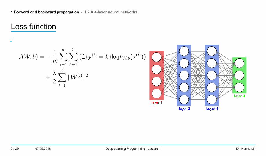
Loss function

-

J(W, b) =−1

m

m∑i=1

3∑k=1

(1{y (i) = k}loghW,b(x (i))

)+λ

2

3∑l=1

||W (l)||2



Partial derivative

-

∆(4) = −(1{y (i) = k} −

eZ(4)∑3

i=1 eZ(4)i

)∂J

∂W (3)= ∆(4)A(3) + λW (3)

∂J

∂b(3)= ∆(4)

∆(3) = ∆(4)W (3)f ′(Z(3))

∂J

∂W (2)= ∆(3)A(2) + λW (2)

∂J

∂b(2)= ∆(3)

∆(2) = ∆(3)W (2)f ′(Z(2))

∂J

∂W (1)= ∆(2) A(1)︸︷︷︸

x

+λW (1)∂J

∂b(1)= ∆(2)


1 Forward and backward propagation - 1.3 Forward propagation

Forward propagation

- From layer l to layer l + 1, the activation is computed as:

Z(l+1) = W (l)A(l) + b(l)

A(l+1) = f (Z(l+1))

- When l = 1, A(1) = x- When l is equal to the number of layers L, f(x) is the cost function of linear model, e.g.,

softmax in previous example


1 Forward and backward propagation - 1.4 Backward propagation

Backward propagation

- From layer l + 1 to layer l , the partial derivative is computed as:∂J

∂W (l)= ∆(l+1)A(l) + λW (l)

∂J

∂b(l)= ∆(l+1)

∆(l) = ∆(l+1)W (l)f ′(Z(l))

- When l = 1, A(1) = x- When l = L, ∆(L) is the partial derivative of linear model


2 Build a L-layer neural networks - 2.1 Training, validation, and test sets

Hyperparameter tuning

- To build a neural network, one must tune a lot of parameters. For example, number oflayers, learning rate of SGD, number of units in each hidden layers, regularizationparameter, ...

- Two options to find optimal parameters:- a separate validation set when you have a large dataset- k-fold cross validation when you have a small dataset

- Q: why cannot use the test set for the purpose of tweaking hyperparameters?



A separate validation set

- Split dataset into three non-overlapping sets, i.e., training set, validation set, and testset. For example, in our assignment, we have 49,000 training data, 1,000 validationdata, and 1,000 test data

- Train your model with training set, and measure the performance on validation set withdifferent parameters, choose the optimal parameters. Namely, the parameters thathas the best performance on validation set

- Measure the performance of your model on test set with the optimal parameter- Pros and cons:

- More bias- Less computational time



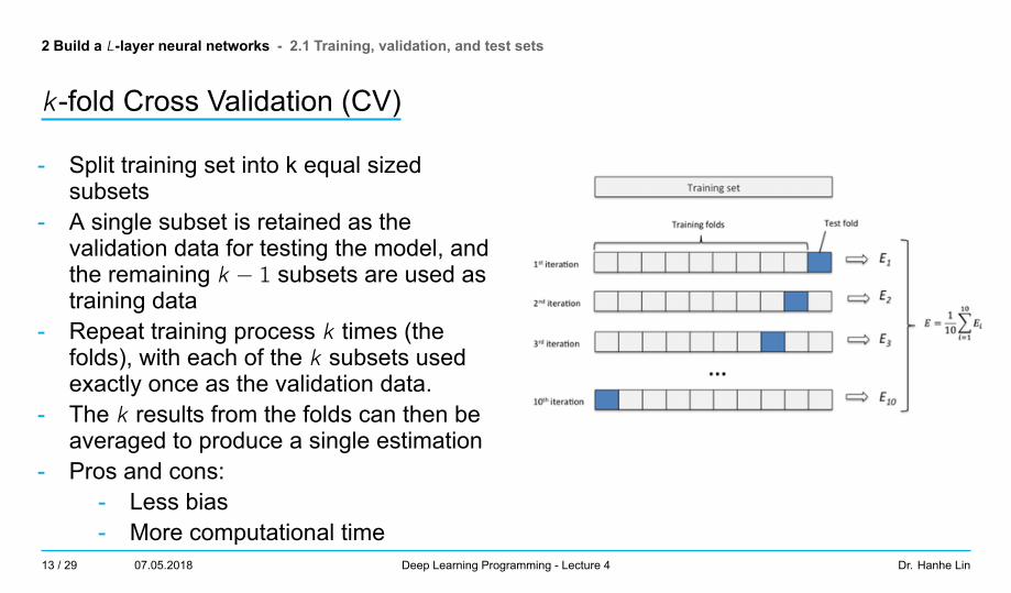
k-fold Cross Validation (CV)

- Split training set into k equal sizedsubsets

- A single subset is retained as thevalidation data for testing the model, andthe remaining k − 1 subsets are used astraining data

- Repeat training process k times (thefolds), with each of the k subsets usedexactly once as the validation data.

- The k results from the folds can then beaveraged to produce a single estimation

- Pros and cons:- Less bias- More computational time



Grid search for hyperparameter tuning

- Suppose we have two hyperparameters to tune, learning rate α and regularizationterm λ, to find the optimal hyperparameters, we

- pick a bunch of values of α- pick a bunch of values of λ- For each pair of α and λ, evaluate the validation error, either K-fold CV on

training set or on validation set- Pick the pair that gives the minimum value of the validation error

- Coarse-to-fine strategy


2 Build a L-layer neural networks - 2.2 Data preprocessing

Motivation

- Each feature has a different scale, whichmay generate an oval shape

- Result: more iterations to converge- Four forms:

- mean subtraction- normalization- PCA- Whitening



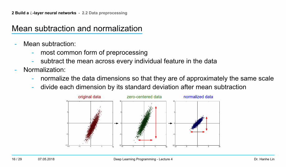
Mean subtraction and normalization

- Mean subtraction:- most common form of preprocessing- subtract the mean across every individual feature in the data

- Normalization:- normalize the data dimensions so that they are of approximately the same scale- divide each dimension by its standard deviation after mean subtraction



PCA

- Principal Component Analysis (PCA) uses orthogonal transformation to convert a setof data of possibly correlated features into a set of values of linearly uncorrelatedfeatures called principal components

- Procedure:- mean subtraction- compute the covariance matrix, which is symmetric and positive semi-definite

with a size of n × n- compute the eigenvectors and eigenvalues of the covariance matrix- project the original (but zero-centered) data into the eigenbasis, namely,

zero-centered data multiply the eigenvectors of the covariance matrix- We could only keep the top k dimensions of the data, e.g., 100, that contain the most

variance so that saving space and time



Whitening

- After computing de-correlated data, the whitening operation divides every dimensionby the eigenvalue to normalize the scale

- Whitened data will be a Gaussian with zero mean and identity covariance matrix



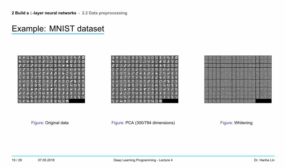
Example: MNIST dataset

Figure: Original data Figure: PCA (300/784 dimensions) Figure: Whitening



Tips

- Data preprocessing should only be computed to training set exclusively, and thenapplied to validation/test data.

- Example: given a training set, compute the data mean, eigenvectors and eigenvaluesof covariance matrix, and keep them for further use. . .

- Data preprocessing is commonly used in traditional machine learning approaches.However, in Convolutional Networks, what we need to do is just to scale the pixelvalue from [0 255] to [0 1], namely, divide by 255


2 Build a L-layer neural networks - 2.3 Weight and bias initialization

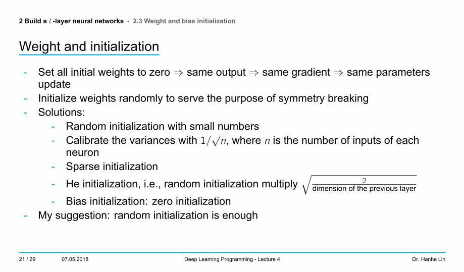
Weight and initialization

- Set all initial weights to zero⇒ same output⇒ same gradient⇒ same parametersupdate

- Initialize weights randomly to serve the purpose of symmetry breaking- Solutions:

- Random initialization with small numbers- Calibrate the variances with 1/

√n, where n is the number of inputs of each

neuron- Sparse initialization- He initialization, i.e., random initialization multiply

√2

dimension of the previous layer

- Bias initialization: zero initialization- My suggestion: random initialization is enough


2 Build a L-layer neural networks - 2.4 Gradient check

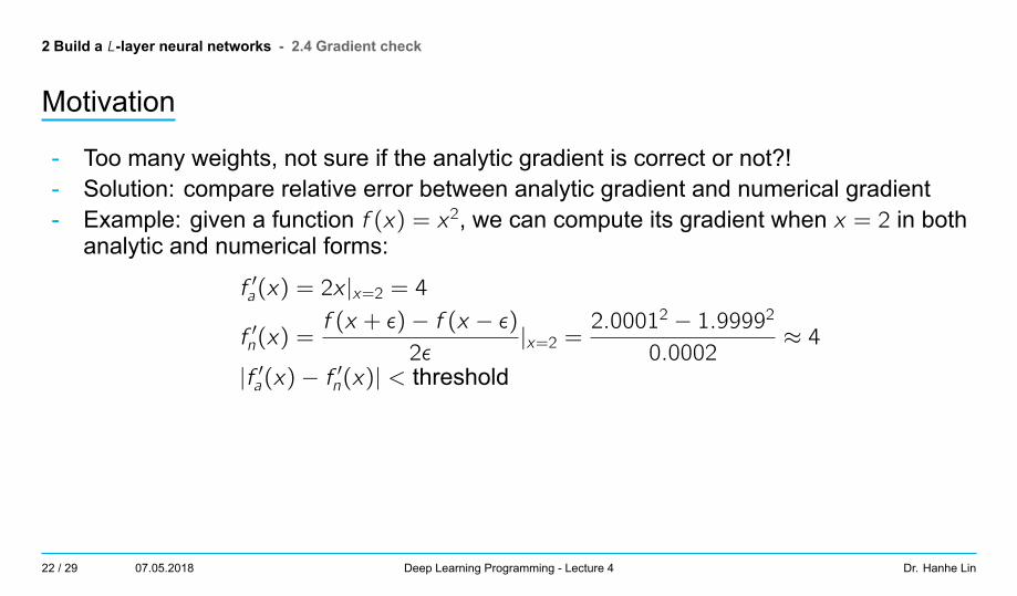
Motivation

- Too many weights, not sure if the analytic gradient is correct or not?!- Solution: compare relative error between analytic gradient and numerical gradient- Example: given a function f (x) = x2, we can compute its gradient when x = 2 in both

analytic and numerical forms:

f ′a(x) = 2x |x=2 = 4

f ′n(x) =f (x + ϵ)− f (x − ϵ)

2ϵ|x=2 =

2.00012 − 1.99992

0.0002≈ 4

|f ′a(x)− f ′n(x)| < threshold



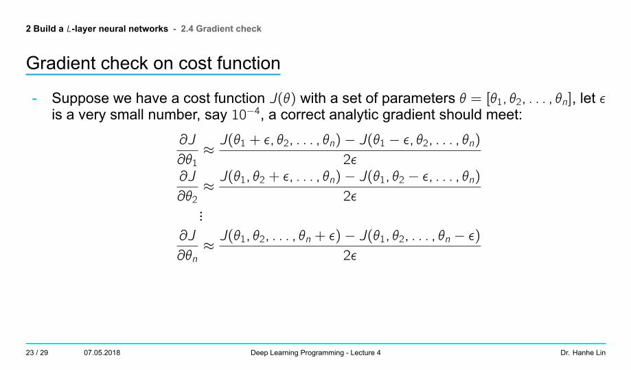
Gradient check on cost function

- Suppose we have a cost function J(θ) with a set of parameters θ = [θ1, θ2, . . . , θn], let ϵis a very small number, say 10−4, a correct analytic gradient should meet:

∂J

∂θ1≈J(θ1 + ϵ, θ2, . . . , θn)− J(θ1 − ϵ, θ2, . . . , θn)

2ϵ∂J

∂θ2≈J(θ1, θ2 + ϵ, . . . , θn)− J(θ1, θ2 − ϵ, . . . , θn)

2ϵ...

∂J

∂θn≈J(θ1, θ2, . . . , θn + ϵ)− J(θ1, θ2, . . . , θn − ϵ)

2ϵ



Tip

- Compute analytic gradient f ′a- Estimate numerical gradient f ′n- Make sure they have a small relative error, say 1e − 7

relative error =|f ′a − f ′n|

max(|f ′a |, |f ′n|)

- Q: why not just use |f ′a − f ′n|?- Gradient check can be generalized to check gradient of any cost function


2 Build a L-layer neural networks - 2.5 Train a neural network model

- Split dataset into training set, validation set, and test set- Design a network architecture according to your application- Train multiple models with different hyperparameters and find the optimal

hyperparameters by validation set:- Randomly initialize weights and biases- Repeat:

- Randomly select a subset of training data, i.e., mini-batch- Forward propagation to compute hypothesis hW,b(x)- Compute cost function J(W, b)- Back propagation to compute partial derivative of weights ∂J

∂W and biases∂J∂b

- Update weights and biases- Train a final model with the optimal hyperparameters and evaluate performance on

test set


3 Deep feedforward neural networks

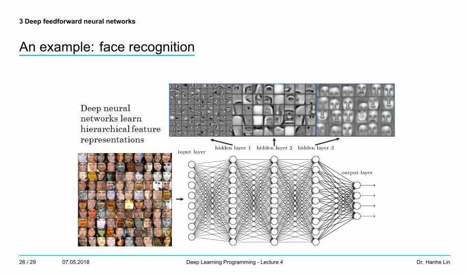
An example: face recognition



Pros and cons

- Pros:- Learn feature and task model simultaneously- Better performance, but not that much

- Cons:- Computational intensive- Non-convex- Prone to overfitting- “Black box” model



Universal approximation properties

- Given enough hidden units, feedforward neural networks with one hidden layer canapproximate any continuous function. However, it

- may not be able to find the right parameters- may find the wrong function as a result of overfitting

- The representational power of feedforward neural network with one hidden layer is thesame as those with multiple hidden layers

- In practice, feedforward neural networks with two hidden layers outperform those withone hidden layer. However, more hidden layers don’t improve that much



Summary

- We extended 3-layer feedforward neural networks to multiple layer feedforward neuralnetworks with forward and backward propagation

- We introduced two ways to tune hyperparameters. If you have a large dataset, it isbetter to split dataset into training, validation, and test sets, whereas if you have asmall dataset, it is better to apply k-fold cross validation

- Data preprocessing is able to make learning faster. However, PCA/Whitening are notused in convolutional neural networks

- Random initialize weights for the purpose of symmetry breaking- Gradient check is very useful when you implement your own cost function


Documents

DeepLearningProgramming Lecture4:Deepneuralnetworks · 24/29 07.05.2018 DeepLearningProgramming-Lecture4 Dr.HanheLin 2Builda L -layerneuralnetworks - 2.5Trainaneuralnetworkmodel -