Data Inspection, Editing, Flagging

AND

RADIO

FREQUENCY

INTERFERENCE (RFI)

Credit: M Gaylard / HartRAO Credit: J. Radcliffe Partially based on A. Offringa’s 2015 ERIS talk

Introduction

Why do we need to edit data??

Radio sources are extremely weak! Remember 1Jy = 10−26 Watts per sq. metre per Hz !

• Brightest sources are ~few 10s Jansky • Mobile phones at 1km away are 108 brighter… • Protected radio bands are exceeded by our bandwidths! • Satellites love to operate at useful radio frequencies.

This is known as Radio Frequency Interference (RFI) and we need to remove it

Introduction

But that’s not all!

• Broken elements (antennas/stations) • Correlator malfunctions • Shadowing • Initial pointing delay • Bandpass issues • Low elevation • Correlated noise on some baselines (e.g. LOFAR split stations)

Introduction

Your source is literally a needle in a haystack!

Data can not be (self-)calibrated when any of these issues are still in the data.

Introduction

Inspection + flagging

Data Averaging (if needed)

Calibration

Imaging

Science!

• Radio Frequency Interference (RFI)

• Data inspection

• Manual data flagging (how to remove sources of bad data)

• Automatic RFI flagging algorithms

• Data averaging

• Sources of imaging errors

Introduction

This talk:

Radio Frequency Interference

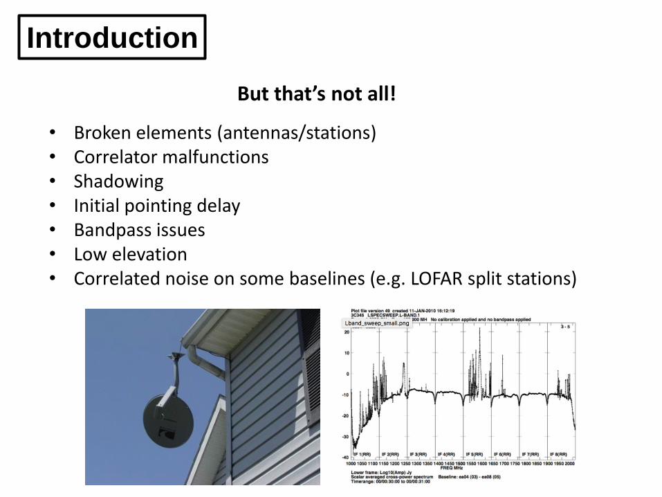
• Radio Frequency Interference (RFI) is a major problem for nearly all radio telescopes.

• Advantage: target source is often much much lower in flux than the RFI source

• Can be generated internally or externally.

• Lots of interference at low frequencies (<1.5 GHz, e.g. LOFAR, GMRT, WSRT, EVLA, MWA, ... )

• Less of an issue for higher frequencies (ALMA); or VLBI but mitigation still required in most cases.

This is what a satellite (IRIDIUM) looks like in data:

Radio Frequency Interference

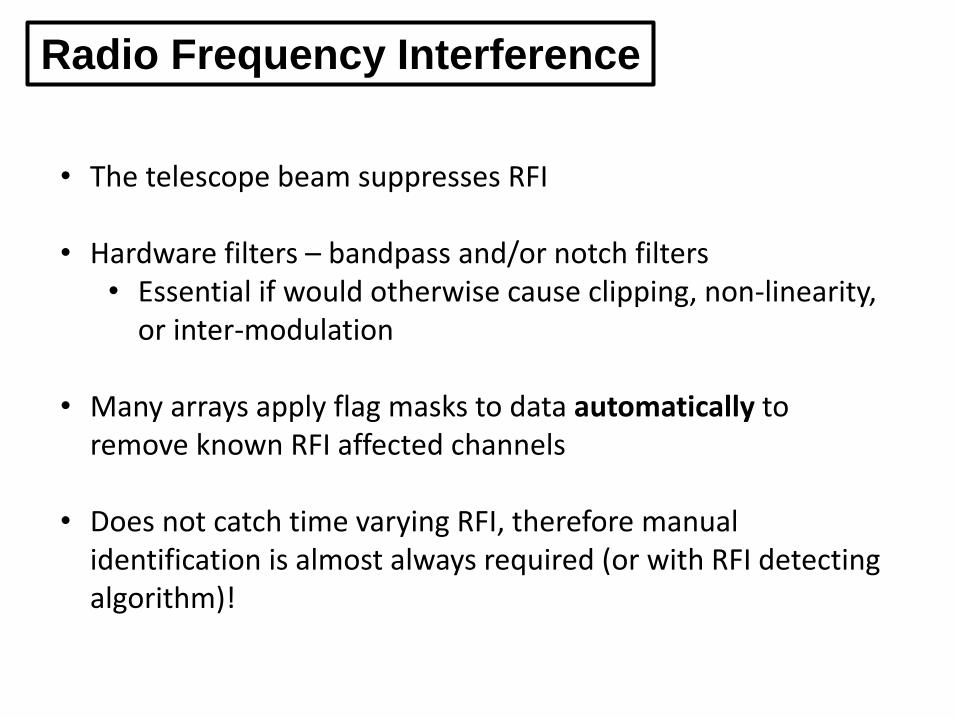
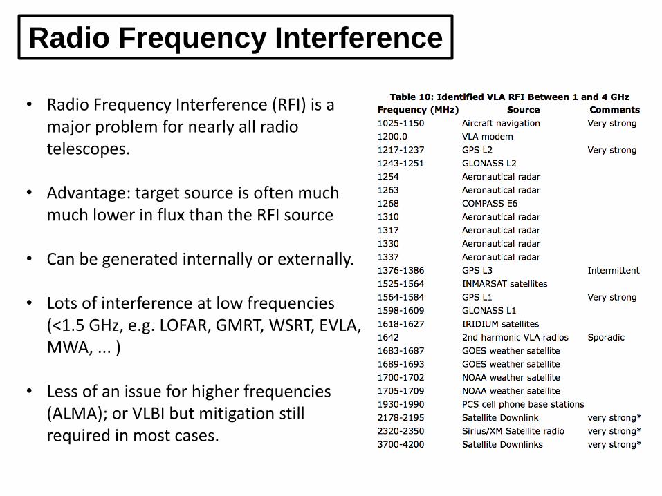
• The telescope beam suppresses RFI

• Hardware filters – bandpass and/or notch filters • Essential if would otherwise cause clipping, non-linearity,

or inter-modulation

• Many arrays apply flag masks to data automatically to remove known RFI affected channels

• Does not catch time varying RFI, therefore manual identification is almost always required (or with RFI detecting algorithm)!

Radio Frequency Interference

Data Inspection

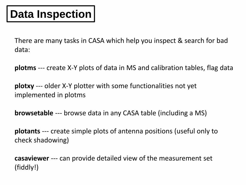
There are many tasks in CASA which help you inspect & search for bad data: plotms --- create X-Y plots of data in MS and calibration tables, flag data plotxy --- older X-Y plotter with some functionalities not yet implemented in plotms browsetable --- browse data in any CASA table (including a MS) plotants --- create simple plots of antenna positions (useful only to check shadowing) casaviewer --- can provide detailed view of the measurement set (fiddly!)

Data Inspection: plotms

plotms - is a very useful tool to identify bad data, gui interface is easy to use!

Can already identify some RFI

Data Inspection: plotms

Can flag interactively in plotms by using the region + flag buttons

Data Inspection: plotms

• A good start! Most of the high amplitude RFI is gone however this is not the most efficient way to flag.

Issues with clipping data

• Noise level varies over time / baseline

• Procedure can be time consuming

• There is more than just very high flux RFI to remove

• What theshold to introduce clip? • Too high a level and some RFI will remain • Too low a level and some uncontaminated data flagged

• Introduces biases to final map

Data Inspection

See a repeating pattern of low fluxes at the start of each scan? We could do this interactively (it could take a while) or we could script it and use flagdata.

Data Flagging

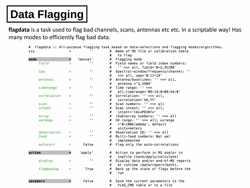
flagdata is a task used to flag bad channels, scans, antennas etc etc. in a scriptable way! Has many modes to efficiently flag bad data.

Data Flagging

Two most important parameters here are mode and action:

Mode determines what sort of flagging needs to be performed (explained later): Action has two options ‘apply’ & ‘calculate’:

• If you use apply, the flags will be applied to the MS. o Setting display = ‘data’ launches an interactive GUI (v. helpful) and the

data flags can be inspected and if unsatisfactory one can exit without applying the flags

o display = ‘report’ prints flagging statistics (can also set display=‘both’ and it doesn both GUI + statistics

• Use ’calculate’ and the flags are calculated but not written to the MS. Useful if

display = ‘data’ so flags can be inspected without straight application

Nb: set flagbackup=True so that the flags are saved to .flagversions file before applying!

Data Flagging

Returning to this data we can find where the bad data is contained and manually flag it using flagdata. This way we ensure that if something should happen to the data we can recover the flags!

Data Flagging: flagdata

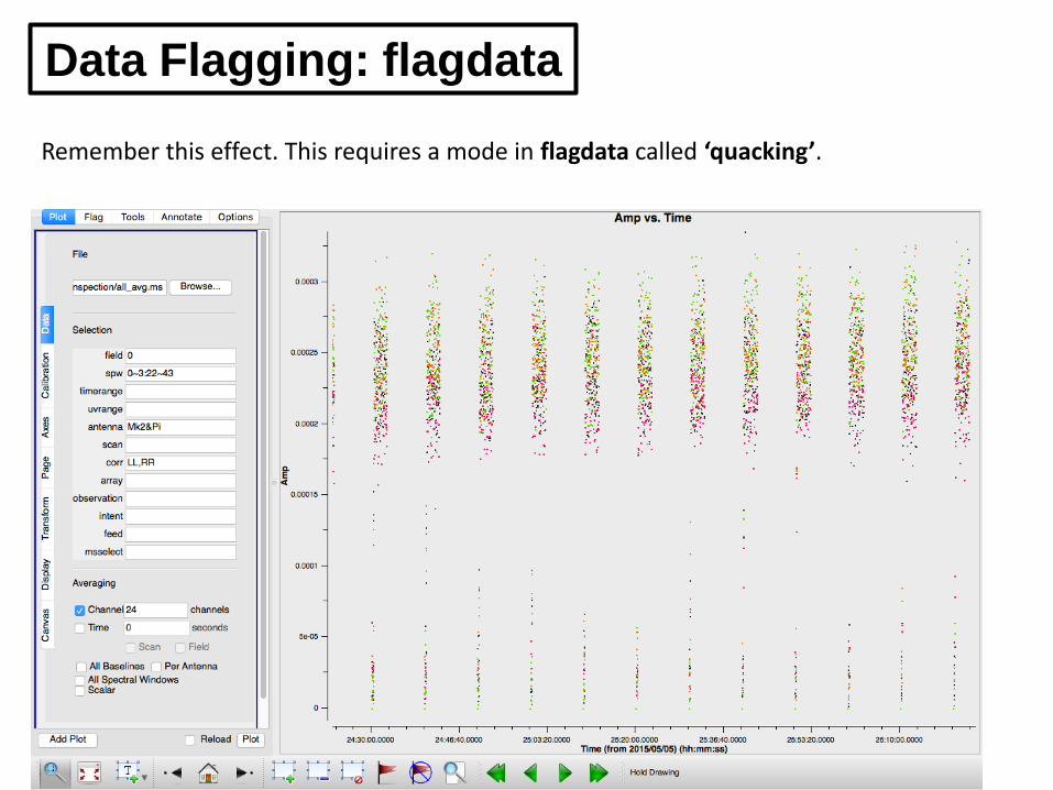
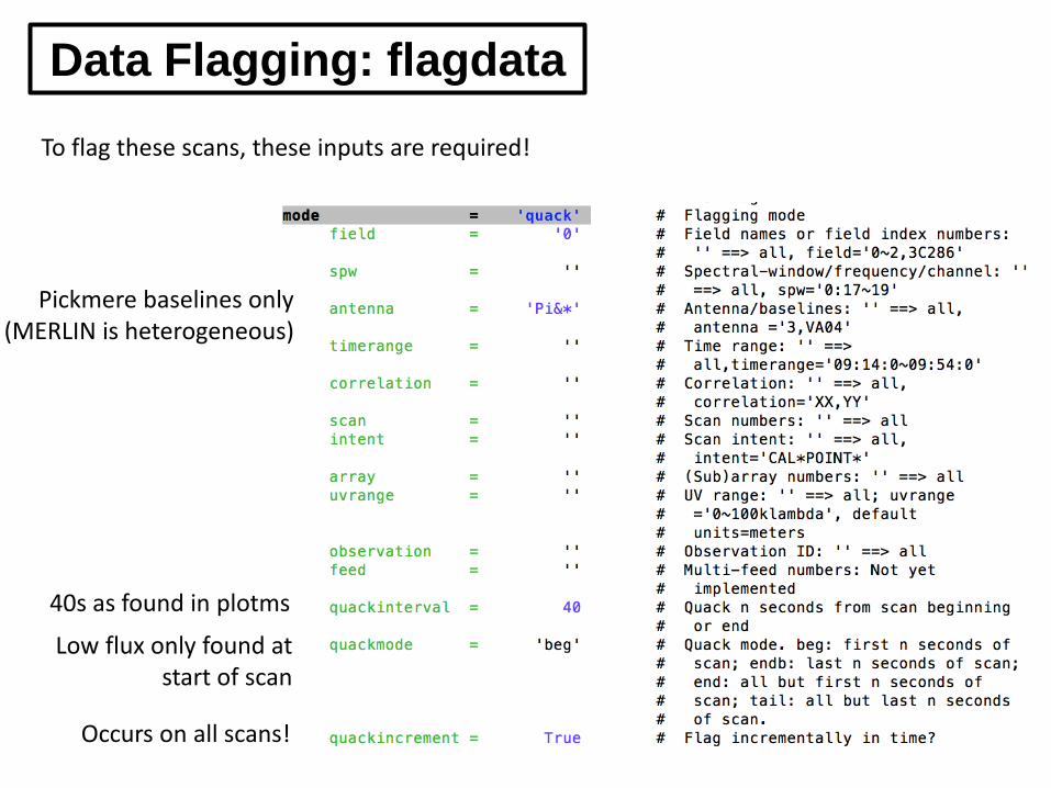
Remember this effect. This requires a mode in flagdata called ‘quacking’.

Data Flagging: flagdata

The low fluxes at the start (and end) are caused by data being recorded when the telescope is being moved between sources.

• Use plotms to approximate the time off source. e.g. here it is 40s • Note that slewing times will be different for non-heterogenous arrays!

Zoom in on two scans

Data Flagging: flagdata

To flag these scans, these inputs are required!

Pickmere baselines only (MERLIN is heterogeneous)

40s as found in plotms

Low flux only found at start of scan

Occurs on all scans!

• Broken elements → remove antennas (flagdata mode = manual)

• Correlator malfunctions → remove timesteps (manual) • Shadowing → remove antennas in time range (shadow) • Initial pointing delay → remove first timesteps (quack) • Bandpass issues → remove channels (manual)

Low elevation → remove antennas with low elevation (elevation)

• Correlated noise on some baselines (e.g. LOFAR split stations) → Flag baselines (manual)

• Interference → remove antennas, timestep, frequencies or baselines... (manual,clip)

Data Flagging: flagdata

If all this is done, then calibrating the data is a whole lot easier!

Automated Data Flagging

We are really good at picking up patterns which allows easy identification of RFI, however computers are not! Common manual excision methods: • Manual selection by data reducing astronomer

• Thresholding / specialized project pipelines (e.g. Baan et al. 2004,

Winkel et al. 2007)

• Manual selection is not practical for modern observatories: • Enormous data volumes, computationally fast algorithms

required. • Needs to be more accurate than thresholding

We need fast automated RFI excision routines!

Two classes of RFI excision methods: • Detection: find & throw away affected data • Filtering or subtracting: estimate RFI contribution and

restore affected data

Detection methods (“flagging”) commonly used • Some specialized pipelines for surveys or instruments

Filtering RFI is harder • Resulting data quality is not well understood • Requires more resources • Lack of full (automated) filtering pipelines

Automated Data Flagging

Automated Data Flagging Example

AOFlagger (Offringa+ 2012)

External package, works with CASA sets (good results reported)

Automated Data Flagging Example

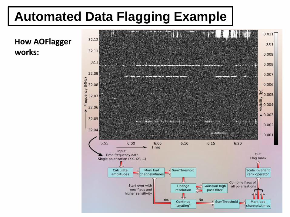
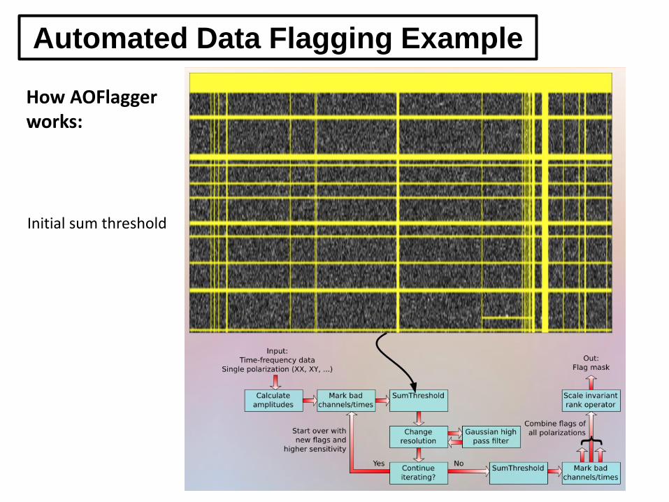
How AOFlagger works:

VarTheshold and SumTheshold

• Look at contiguous subsets of data (in t or f) • Define variable theshold levels for different numbers of

samples in subset

• E.g. Consider data 1 2 14 1 12 2 1

444

• Do cut with 𝜒1 = 5; removes high single values

• None in this case • Do cut with 𝜒2 = 3; removes regions with all values

higher than theshold • Flags the final column • Leaves the other instance of 4 unflagged

• VarTheshold based on absolute values of subset • SumTheshold based on sums of subset (better)

Automated Data Flagging Example

How AOFlagger works:

Initial sum threshold

Automated Data Flagging Example

• Change time & frequency resolution then remove components using high pass filter • Iterate, changing resolution each time

Automated Data Flagging Example

Finish iterating & do final sum threshold

Scale Invariant Rank operator

a) isolated RFI feature b) noise added; part of the feature becomes undetectable c) flagged with the SumThreshold method d) SIR operator applied, parameter η = 0.2.

a) b) c) d)

Automated Data Flagging Example

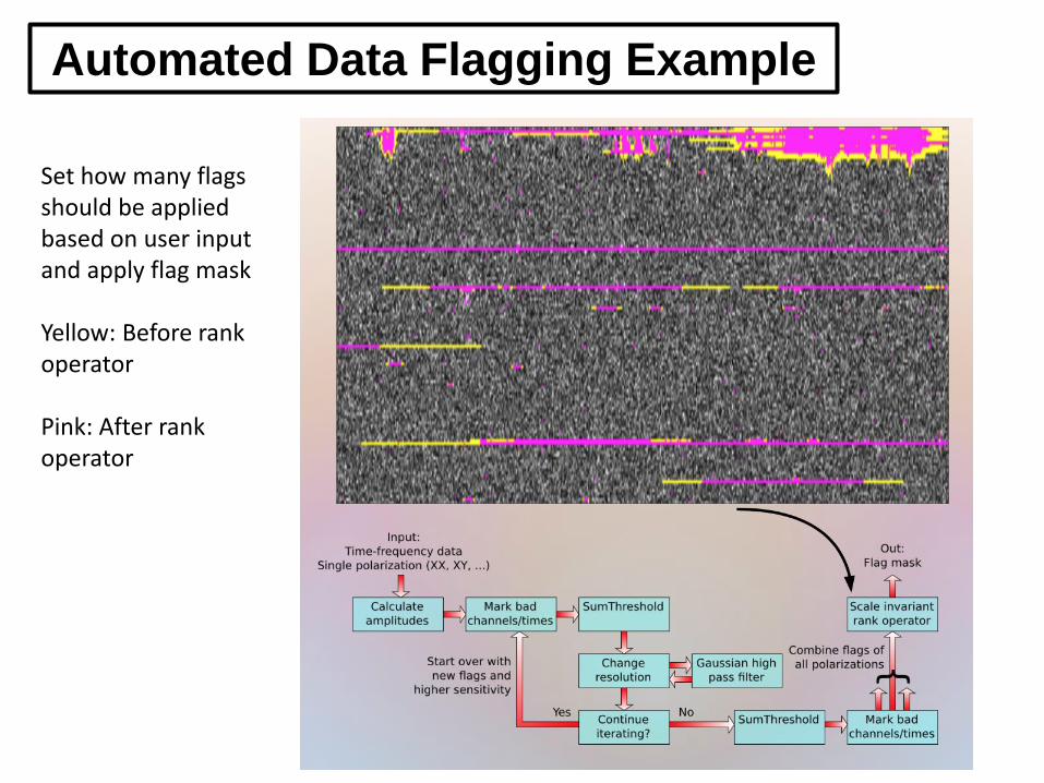
Set how many flags should be applied based on user input and apply flag mask Yellow: Before rank operator Pink: After rank operator

What could go wrong? • Some astronomical sources vary quickly in time (sun,

pulsars, ...)

• Quick fringes are line-like patterns

• Spectral line observations Mostly not an issue – sources are mostly much weaker than RFI, and invisible in single correlations.

Automated Data Flagging Example

Data Averaging

HEALTH WARNING: Always flag (first) at highest possible resolution! Highest resolution: Averaged without RFI detection: • Flagging is incremental: don't reset flags!

• Correlator might have set flags. These will be lost. To undo

flagging, use backup (column).

Data Averaging

• Data size can be reduced by averaging data in time and/or frequency direction

• Only average after RFI detection

• Over-averaging causes smearing • Time-smearing: in tangential direction • Frequency-smearing: in radial direction

• Calibration might also constrain averaging factor

• For high dynamic range may need to calculate and store a

data weight and mean observation time

Rejection from smearing

• Additional rejection effect for sources outside telescope beam • Arises from averaging (f or t) over phase wrapping

• Fringes from a point source • Always have some averaging

• Correlator dump time • Frequency channel width

• Complex visibilities have different phases

• Amplitude suppressed • Degree of reduction depends on

• baseline length • Position in uv-plane

• Sources appear elongated in map

Visibility phase in uv-plane for offset point source

BANDWIDTH SMEARING

Effect is radial smearing, corresponding to radial extent of measurements in uv plane

Example

NVSS image

e-MERLIN

(from Basic Imaging Lecture)

• Time-average smearing (de-correlation) produces tangential smearing

• Not easily parameterized. At declination +90° a simple case exists where percentage time smearing is given by:

• At other declinations, the effects are more complicated.

TIME SMEARING

Not smeared

Smeared

(from Basic Imaging Lecture)

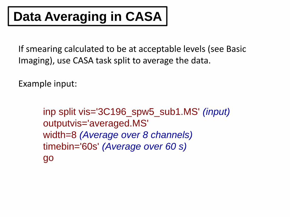
inp split vis='3C196_spw5_sub1.MS' (input)

outputvis='averaged.MS'

width=8 (Average over 8 channels)

timebin='60s' (Average over 60 s)

go

Data Averaging in CASA

If smearing calculated to be at acceptable levels (see Basic Imaging), use CASA task split to average the data. Example input:

Original resolution: After averaging

Data Averaging in CASA

• Processing data can be very time expensive, but almost all steps scale linear with number of visibilities.

• Work on averaged data (and/or subset) while experimenting with settings

• May be necessary to calculate mean observing time and weight

Exploiting coherence of interference

• RFI clipping works on data amplitudes • Ignores phase information

• Consider an interferometer with no phase tracking: • Map centre corresponds to point on the sky where fringe

rate is always zero. • For a ground mounted interferometer this point is the

North (or South) Pole. • Where the telescope is pointing is (largely) irrelevant to

this • Apply fringe rotation to shift the phase centre (i.e. where

the map is centre). • This can be anywhere, but often the pointing centre • Slowly varying contaminating signals map to the Pole.

• Can also apply a fringe rate filter…

Recap: fringe rate I

• When observing a source, there is a path difference between the two antennas

• While tracking a source on the sky the path difference between two antennas changes

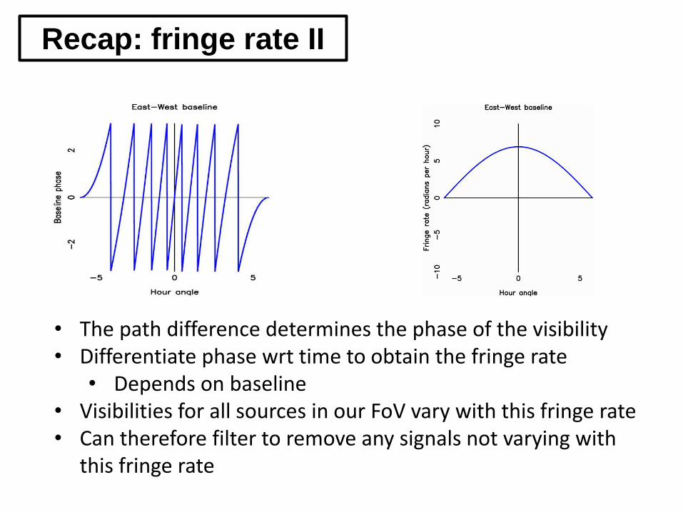
Recap: fringe rate II

• The path difference determines the phase of the visibility • Differentiate phase wrt time to obtain the fringe rate

• Depends on baseline • Visibilities for all sources in our FoV vary with this fringe rate • Can therefore filter to remove any signals not varying with

this fringe rate

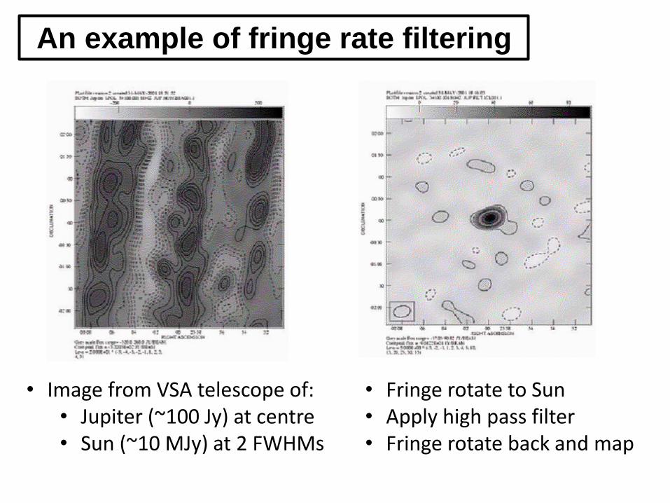
An example of fringe rate filtering

• Image from VSA telescope of: • Jupiter (~100 Jy) at centre • Sun (~10 MJy) at 2 FWHMs

• Fringe rotate to Sun • Apply high pass filter • Fringe rotate back and map

Summary

• First step in data processing is data inspection

• Second step is BACKUP YOUR DATA

• Third step is data flagging and RFI detection

• Calibration, imaging, ... to be discussed!