Embed Size (px)
Citation preview

Data-Driven Penalty Calibration: Slope Heuristics andthe capushe Package
Jean-Patrick Baudry
Universite Paris-Sud 11Project select (INRIA)
UPMC
Joint work with C. Maugis & B. Michel
September 3, 2010
J.-P. Baudry September 3, 2010 1 / 20

Table of Contents
1 Contrast Minimization
2 Model Selection and Penalized Criteria
3 Slope Heuristics and the capushe Package
4 Conclusion and Perspectives
J.-P. Baudry September 3, 2010 2 / 20

Contrast Minimization General Settings
X1, . . . ,Xn, . . . i.i.d. from an unknown distribution.
s a function of interest linked to this distribution.
The contrast minimization approach relies on an empirical contrastγn, depending on X1, . . . ,Xn and such that
t 7→ E[γn(t)]
reaches a minimum value at t = s.
In any model S , s is estimated by the empirical contrast minimizer
s ∈ argmint∈S
γn(t).
Its quality is measured by the corresponding natural loss function `:
∀t ∈ S , `(s, t) = E[γn(t)]− E[γn(s)].
J.-P. Baudry September 3, 2010 3 / 20
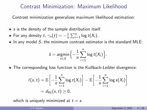
Contrast Minimization: Maximum Likelihood
Contrast minimization generalizes maximum likelihood estimation:
s is the density of the sample distribution itself.
For any density t, γn(t) = − 1n
∑ni=1 log t(Xi ).
In any model S , the minimum contrast estimator is the standard MLE:
s = argmint∈S
{−1
n
n∑i=1
log t(Xi )}.
The corresponding loss function is the Kullback-Leibler divergence:
`(s, t) = E[−1
n
n∑i=1
log t(Xi )
]− E
[−1
n
n∑i=1
log s(Xi )
]= dKL(s, t) ≥ 0,
which is uniquely minimized at t = s.
J.-P. Baudry September 3, 2010 4 / 20

Contrast Minimization: Other Contrasts
Examples of least-squares constrasts.
• Regression
Yi = s(Xi ) + εi , i = 1, . . . , n
γn(t) = − 1n
∑ni=1
(Yi − t(Xi )
)2
`(s, t) = 1n
∑ni=1 E
[(t − s)2(Xi )
]≥ 0
• Gaussian white noise
dY (n)(x) = s(x)dx + 1√
ndW (x),
with W a brownian motion
γn(t) = ‖t‖2 − 2∫
t(x)dY (n)(x)
`(s, t) = ‖t − s‖22 ≥ 0
• Density Estimation
X1, . . . ,Xn i.i.d. with density s
γn(t) = ‖t‖2 − 2n
∑ni=1 t(Xi )
`(s, t) = ‖t − s‖22 ≥ 0
J.-P. Baudry September 3, 2010 5 / 20
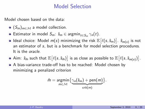
Model Selection
Model chosen based on the data:
(Sm)m∈M a model collection.
Estimator in model Sm: sm ∈ argmint∈Sm γn(t).
Ideal choice: Model m(s) minimizing the risk E[`(s, sm)
]. sm(s) is not
an estimator of s, but is a benchmark for model selection procedures.It is the oracle.
Aim: sm such that E[`(s, sm)
]is as close as possible to E
[`(s, sm(s))
].
A bias-variance trade-off has to be reached: Model chosen byminimizing a penalized criterion
m = argminm∈M
{γn(sm) + pen(m)︸ ︷︷ ︸
crit(m)
}.
J.-P. Baudry September 3, 2010 6 / 20

Model Selection: Ideal PenaltyLet us denote
sD = argmin{sm:m∈M,Dim(m)=D}
γn(sm).
sD = argmint∈
⋃Dim(m)=D
Sm
E[γn(t)
].
crit(D) = γn(sD) + pen(D)(−γn(s)
)= γn(sD)− γn(s)︸ ︷︷ ︸
≈`(s,sD)
−(γn(sD)− γn(sD)︸ ︷︷ ︸
vD
)+ pen(D)
→ With the ideal penalty
penid(D) = vD + `(s, sD)− `(s, sD)︸ ︷︷ ︸`(sD ,sD)
,
critid(D) ≈ `(s, sD) selects the oracle.
J.-P. Baudry September 3, 2010 7 / 20

Model Selection: Penalized Criteria
Recall: penid(D) = vD + `(sD , sD).
Asymptotic approach:
Akaike’s AIC (73), density estimation with log-likelihood contrast:
`(sD , sD) ≈ vD ≈D
2n.
penAIC (D) =1
nD
Mallows’ Cp (73), least-square regression:
penCp(D) = 2σ2
nD
The models dimension and the number of models are bounded, andn→∞.
J.-P. Baudry September 3, 2010 8 / 20

Model Selection: Penalized Criteria
Recall: penid(D) = vD + `(sD , sD).
Nonasymptotic approach:
Models, models dimension and number of models may depend on n.
Example: Change Points Detection. Regression by piecewise constantfunctions with endpoints to be chosen on the grid
{ jn : 0 ≤ j ≤ n
}.
Birge & Massart (97, 01, 07) and others get nonasymptotic bounds onvD + `(sD , sD) through concentration results on empirical processes.
They derive “optimal” penalties typically such that
pen(D) = κD
or pen(D) = κD(
2 + log(nD
))(Lebarbier, 05)
But κ is unknown and may depend on s, the sample distribution...
J.-P. Baudry September 3, 2010 9 / 20

Slope Heuristics: Data-driven Penalty Calibration
Recall: crit(D) ≈ γn(sD)− γn(sD)︸ ︷︷ ︸`(s,sD )−vD
+pen(D)
→ With the penalty (α > 0)
penα(D) = αvD
= ακminD, (for example)
critα(D) = `(s, sD) + (α− 1)vD selects models among the mostcomplex iff α < 1.
“penmin = vD is a minimal penalty”.
→ Deduce the optimal penalty (vD ≈ `(sD , sD))
penopt = 2× penmin
= 2ακminD. (for example)
(Birge & Massart, 07 ; Arlot & Massart, 09)
J.-P. Baudry September 3, 2010 10 / 20
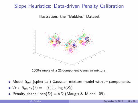
Slope Heuristics: Data-driven Penalty Calibration
Illustration: the “Bubbles” Dataset
−4
−2
0
2
4
6
8
10
−4
−2
0
2
4
6
8
10−4
−3
−2
−1
0
1
2
3
4
1000-sample of a 21-component Gaussian mixture.
Model Sm: (spherical) Gaussian mixture model with m components.
∀t ∈ Sm, γn(t) = −∑n
i=1 log t(Xi ).
Penalty shape: pen(D) = κD (Maugis & Michel, 09).
J.-P. Baudry September 3, 2010 11 / 20

capushe(Baudry, Maugis, Michel, 10)
J.-P. Baudry September 3, 2010 12 / 20

Slope Heuristics: Dimension Jump
J.-P. Baudry September 3, 2010 13 / 20

Slope Heuristics: Dimension Jump
Thresholding the jump(Arlot & Massart, 09)
J.-P. Baudry September 3, 2010 14 / 20
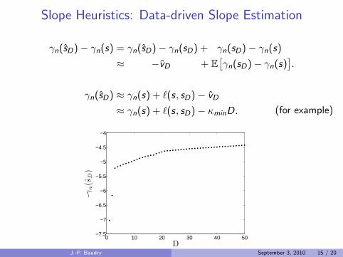
Slope Heuristics: Data-driven Slope Estimation
γn(sD)− γn(s) = γn(sD)− γn(sD) + γn(sD)− γn(s)
≈ −vD + E[γn(sD)− γn(s)
].
γn(sD) ≈ γn(s) + `(s, sD)− vD
≈ γn(s) + `(s, sD)− κminD. (for example)
0 10 20 30 40 50−7.5
−7
−6.5
−6
−5.5
−5
−4.5
−4
-γn(s
D)
DJ.-P. Baudry September 3, 2010 15 / 20

Slope Heuristics: Data-driven Slope Estimation
Recall: γn(sD) ≈ γn(s) + `(s, sD)− κminD.
J.-P. Baudry September 3, 2010 16 / 20

Slope Heuristics: Data-driven Slope Estimation
Comparing robust and simple regression
J.-P. Baudry September 3, 2010 17 / 20

“Bubbles” Experiment: Results
m 3–4 15–18 19 20 21 22 23 24 25 ≥ 35 Risk ratio
Or. 1 76 15 3 3 2 1AIC 100 2.59BIC 3 6 23 57 9 1 1 1.17DDSE 3 7 59 20 6 3 2 1.06DJ 6 3 7 59 18 2 3 2 1.49
Table: Number of times a model m is selected among the 100 simulations byAIC, BIC, the data-driven slope estimation method (DDSE) and the dimensionjump method (DJ). The last column is the ratio between the risk of the selectedestimator and the oracle risk.
J.-P. Baudry September 3, 2010 18 / 20

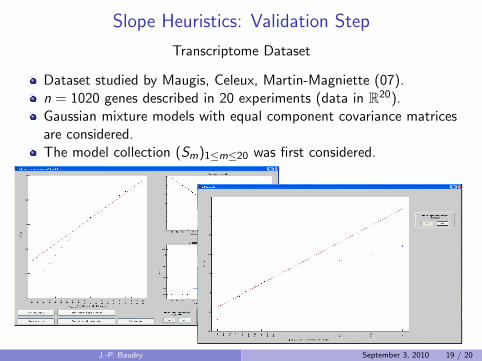
Slope Heuristics: Validation Step
Transcriptome Dataset
Dataset studied by Maugis, Celeux, Martin-Magniette (07).
n = 1020 genes described in 20 experiments (data in R20).
Gaussian mixture models with equal component covariance matricesare considered.
The model collection (Sm)1≤m≤20 was first considered.
J.-P. Baudry September 3, 2010 19 / 20
Slope Heuristics: Validation Step
Transcriptome Dataset
Dataset studied by Maugis, Celeux, Martin-Magniette (07).n = 1020 genes described in 20 experiments (data in R20).Gaussian mixture models with equal component covariance matricesare considered.The model collection (Sm)1≤m≤20 was first considered.
J.-P. Baudry September 3, 2010 19 / 20

Slope Heuristics: Validation Step
Transcriptome Dataset
Dataset studied by Maugis, Celeux, Martin-Magniette (07).n = 1020 genes described in 20 experiments (data in R20).Gaussian mixture models with equal component covariance matricesare considered.The model collection (Sm)1≤m≤60 has been eventually considered.
J.-P. Baudry September 3, 2010 19 / 20
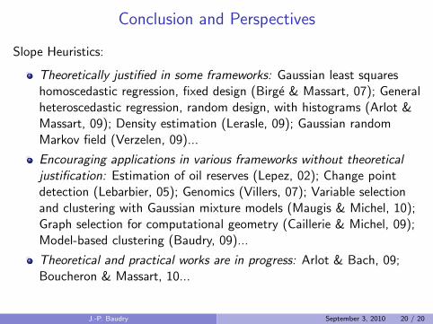
Conclusion and Perspectives
Slope Heuristics:
Theoretically justified in some frameworks: Gaussian least squareshomoscedastic regression, fixed design (Birge & Massart, 07); Generalheteroscedastic regression, random design, with histograms (Arlot &Massart, 09); Density estimation (Lerasle, 09); Gaussian randomMarkov field (Verzelen, 09)...
Encouraging applications in various frameworks without theoreticaljustification: Estimation of oil reserves (Lepez, 02); Change pointdetection (Lebarbier, 05); Genomics (Villers, 07); Variable selectionand clustering with Gaussian mixture models (Maugis & Michel, 10);Graph selection for computational geometry (Caillerie & Michel, 09);Model-based clustering (Baudry, 09)...
Theoretical and practical works are in progress: Arlot & Bach, 09;Boucheron & Massart, 10...
J.-P. Baudry September 3, 2010 20 / 20

Thank you for attention!
J.-P. Baudry September 3, 2010 21 / 20
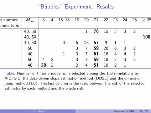
“Bubbles” Experiment: Results
Selected number Mmax 3 4 15–18 19 20 21 22 23 24 25 ≥ 35 Riskof components m ratio
Oracle 40, 50 1 76 15 3 3 2 1AIC 40, 50 100 2.59BIC 40, 50 3 6 23 57 9 1 1 1.17DDSE 50 3 7 59 20 6 3 2 1.06DDSE 40 1 3 7 61 18 4 4 2 1.09DJ 50 4 2 3 7 59 18 2 3 2 1.49DJ 40 28 2 2 4 51 10 2 1 3.27
Table: Number of times a model m is selected among the 100 simulations byAIC, BIC, the data-driven slope estimation method (DDSE) and the dimensionjump method (DJ). The last column is the ratio between the risk of the selectedestimator by each method and the oracle risk.
J.-P. Baudry September 3, 2010 22 / 20
![Convex Optimization CMU-10725 · Definition [Penalty function] Example [Penalty function] 18 Derivative of the penalty function Penalty program: Penalty function: Assumptions: Derivatives:](https://img.dokumen.tips/doc/110x75/5f4d6fd89079d1731710faab/convex-optimization-cmu-definition-penalty-function-example-penalty-function.jpg)