Data analysis and processing techniques for remaining

Rowan University Rowan University

Rowan Digital Works Rowan Digital Works

Theses and Dissertations

6-5-2017

Data analysis and processing techniques for remaining useful life Data analysis and processing techniques for remaining useful life

estimations estimations

John Scott Bucknam Rowan University

Follow this and additional works at: https://rdw.rowan.edu/etd

Part of the Computer Sciences Commons, and the Operations Research, Systems Engineering and

Industrial Engineering Commons

Recommended Citation Recommended Citation Bucknam, John Scott, "Data analysis and processing techniques for remaining useful life estimations" (2017). Theses and Dissertations. 2430. https://rdw.rowan.edu/etd/2430

This Thesis is brought to you for free and open access by Rowan Digital Works. It has been accepted for inclusion in Theses and Dissertations by an authorized administrator of Rowan Digital Works. For more information, please contact [email protected].

https://rdw.rowan.edu/

https://rdw.rowan.edu/etd

https://rdw.rowan.edu/etd?utm_source=rdw.rowan.edu%2Fetd%2F2430&utm_medium=PDF&utm_campaign=PDFCoverPages

http://network.bepress.com/hgg/discipline/142?utm_source=rdw.rowan.edu%2Fetd%2F2430&utm_medium=PDF&utm_campaign=PDFCoverPages



https://rdw.rowan.edu/etd/2430?utm_source=rdw.rowan.edu%2Fetd%2F2430&utm_medium=PDF&utm_campaign=PDFCoverPages

mailto:[email protected]

DATA ANALYSIS AND PROCESSING TECHNIQUES FOR REMAININGUSEFUL LIFE ESTIMATIONS

byJohn S. Bucknam Jr.

A Thesis

Submitted to theDepartment of Computer Science

College of Science and Mathematicsin partial fulfillment of the requirement

for the degree ofMaster of Science in Computer Science

atRowan University

May 26, 2017

Thesis Chair: Ganesh Baliga, PhD.

c© 2017 John S. Bucknam Jr.

Acknowledgments

I would like to thank Dr. Ganesh Baliga for keeping on track as I finished this paper,

as well as Nick LaPosta for those 2:00 AM moments. I would also like to thank my family

for supporting me throughout my Bachelors and Masters.

iii

Abstract

John S. Bucknam Jr.DATA ANALYSIS AND PROCESSING TECHNIQUES FOR REMAINING USEFUL

LIFE ESTIMATIONS2016-2017

Ganesh Baliga, PhD.Master of Science in Computer Science

In the field of engineering, it is important to understand different engineering sys-

tems and components, not only in how they currently performs, but also how their per-

formance degrades over time. This extends to the field of prognostics, which attempts to

predict the future of a system or component based on its past and present states. A com-

mon problem in this field is the estimation of remaining useful life, or how long a system or

component functionality will last. The well-known datasets for this problem are the PHM

and C-MAPSS datasets. These datasets contain simulated sensor data for different turbofan

engines generated over time, and have been used to study estimations of remaining useful

life.

In thesis, we study estimations of remaining useful life using different methods of

data analytics, preprocessing, post-processing, different target functions used for training

models, and their combinations. We compared their performance primarily using scores

from the 2008 Prognostics and Health Management Competition. Our basic feedforward

neural network with aggregation outperforms previously competitors and other modern

methods. Our results also gave us a ranking between the top 10 and 15 based on a 2014

benchmark using the PHM dataset. We have improved the results of previously, published

methods, primarily focusing on the Prognostics Health Management competition score of

our results for better comparisons.

iv

Table of Contents

Abstract . . . . . . . . . . . . . . . . . . . . . . . . . . . . . . . . . . . . . . . . . iv

List of Figures . . . . . . . . . . . . . . . . . . . . . . . . . . . . . . . . . . . . . . viii

List of Tables . . . . . . . . . . . . . . . . . . . . . . . . . . . . . . . . . . . . . . xi

Chapter 1: Introduction . . . . . . . . . . . . . . . . . . . . . . . . . . . . . . . . 1

1.1 Background . . . . . . . . . . . . . . . . . . . . . . . . . . . . . . . . . . 1

1.2 Problem Description . . . . . . . . . . . . . . . . . . . . . . . . . . . . . 2

1.3 Motivation . . . . . . . . . . . . . . . . . . . . . . . . . . . . . . . . . . . 4

1.4 Current Methods . . . . . . . . . . . . . . . . . . . . . . . . . . . . . . . 5

Chapter 2: Understanding the Data and Experiments . . . . . . . . . . . . . . . . . 8

2.1 General Information . . . . . . . . . . . . . . . . . . . . . . . . . . . . . . 8

2.2 RUL Target Function . . . . . . . . . . . . . . . . . . . . . . . . . . . . . 11

2.3 Fault Mode . . . . . . . . . . . . . . . . . . . . . . . . . . . . . . . . . . 13

2.4 Operating Conditions . . . . . . . . . . . . . . . . . . . . . . . . . . . . . 15

2.5 Testing Data . . . . . . . . . . . . . . . . . . . . . . . . . . . . . . . . . . 18

2.6 Experiment Layout . . . . . . . . . . . . . . . . . . . . . . . . . . . . . . 19

2.6.1 Model layout. . . . . . . . . . . . . . . . . . . . . . . . . . . . . 20

Chapter 3: Data and Target Function Processing . . . . . . . . . . . . . . . . . . . 22

3.1 Overview . . . . . . . . . . . . . . . . . . . . . . . . . . . . . . . . . . . 22

3.2 Basic Normalization . . . . . . . . . . . . . . . . . . . . . . . . . . . . . 24

3.3 Regime Partitioning . . . . . . . . . . . . . . . . . . . . . . . . . . . . . . 26

3.3.1 Clustering. . . . . . . . . . . . . . . . . . . . . . . . . . . . . . . 29

3.3.2 Purpose. . . . . . . . . . . . . . . . . . . . . . . . . . . . . . . . 30

3.3.3 Issues. . . . . . . . . . . . . . . . . . . . . . . . . . . . . . . . . 31

3.4 Data Selection . . . . . . . . . . . . . . . . . . . . . . . . . . . . . . . . . 31

3.5 Filtering and Aggregation . . . . . . . . . . . . . . . . . . . . . . . . . . . 32

v

Table of Contents (Continued)

3.5.1 Regression. . . . . . . . . . . . . . . . . . . . . . . . . . . . . . . 33

3.5.2 Kalman filters. . . . . . . . . . . . . . . . . . . . . . . . . . . . . 34

3.5.3 Butterworth filter. . . . . . . . . . . . . . . . . . . . . . . . . . . 34

3.5.4 Savitzky-Golay filter. . . . . . . . . . . . . . . . . . . . . . . . . 34

3.6 Target Function Transformations . . . . . . . . . . . . . . . . . . . . . . . 35

3.6.1 Kinked function. . . . . . . . . . . . . . . . . . . . . . . . . . . . 36

3.6.2 Scaled target function. . . . . . . . . . . . . . . . . . . . . . . . . 36

Chapter 4: Experiments . . . . . . . . . . . . . . . . . . . . . . . . . . . . . . . . 38

4.1 Baseline Models . . . . . . . . . . . . . . . . . . . . . . . . . . . . . . . . 38

4.1.1 Results. . . . . . . . . . . . . . . . . . . . . . . . . . . . . . . . 39

4.2 Max-Multiplier Experiment . . . . . . . . . . . . . . . . . . . . . . . . . . 40

4.2.1 Hypothesis. . . . . . . . . . . . . . . . . . . . . . . . . . . . . . 40

4.2.2 Methodology. . . . . . . . . . . . . . . . . . . . . . . . . . . . . 40

4.2.3 Results. . . . . . . . . . . . . . . . . . . . . . . . . . . . . . . . 41

4.3 Cycle Number Inclusion Experiment . . . . . . . . . . . . . . . . . . . . . 42

4.3.1 Hypothesis. . . . . . . . . . . . . . . . . . . . . . . . . . . . . . 42

4.3.2 Methodology. . . . . . . . . . . . . . . . . . . . . . . . . . . . . 42

4.3.3 Results. . . . . . . . . . . . . . . . . . . . . . . . . . . . . . . . 43

4.4 Classifiers Exploration . . . . . . . . . . . . . . . . . . . . . . . . . . . . 43

4.4.1 Hypothesis. . . . . . . . . . . . . . . . . . . . . . . . . . . . . . 45

4.4.2 Methodology. . . . . . . . . . . . . . . . . . . . . . . . . . . . . 45

4.4.3 Results. . . . . . . . . . . . . . . . . . . . . . . . . . . . . . . . 46

4.5 Regime Partitioning . . . . . . . . . . . . . . . . . . . . . . . . . . . . . . 47

4.5.1 Hypothesis. . . . . . . . . . . . . . . . . . . . . . . . . . . . . . 48

4.5.2 Methodology. . . . . . . . . . . . . . . . . . . . . . . . . . . . . 48

vi

Table of Contents (Continued)

4.5.3 Results. . . . . . . . . . . . . . . . . . . . . . . . . . . . . . . . 49

4.6 Aggregation via Filtering . . . . . . . . . . . . . . . . . . . . . . . . . . . 54

4.6.1 Hypothesis. . . . . . . . . . . . . . . . . . . . . . . . . . . . . . 54

4.6.2 Methodology. . . . . . . . . . . . . . . . . . . . . . . . . . . . . 54

4.6.3 Results. . . . . . . . . . . . . . . . . . . . . . . . . . . . . . . . 55

Chapter 5: Conclusion . . . . . . . . . . . . . . . . . . . . . . . . . . . . . . . . . 62

5.1 Future Work . . . . . . . . . . . . . . . . . . . . . . . . . . . . . . . . . . 63

5.1.1 Transferability of datasets. . . . . . . . . . . . . . . . . . . . . . . 63

5.1.2 Searching for a better scaling multiplier. . . . . . . . . . . . . . . 63

5.1.3 Incrementing our target function. . . . . . . . . . . . . . . . . . . 64

5.1.4 Preprocessed aggregation. . . . . . . . . . . . . . . . . . . . . . . 65

References . . . . . . . . . . . . . . . . . . . . . . . . . . . . . . . . . . . . . . . . 66

vii

List of Figures

Figure Page

Figure 1. Scoring Equation . . . . . . . . . . . . . . . . . . . . . . . . . . . . . 3

Figure 2. C-MAPSS 1 - Unit 1 Sensors Example (Expanded Normalization from

chapter 3) . . . . . . . . . . . . . . . . . . . . . . . . . . . . . . . . . . . 11

Figure 5. RUL Equation . . . . . . . . . . . . . . . . . . . . . . . . . . . . . . . 12

Figure 3. Cycle Number of Data Points in PHM TRAIN Unit 1 . . . . . . . . . . 12

Figure 4. RUL Target of Data Points in PHM TRAIN Unit 1 . . . . . . . . . . . . 12

Figure 6. C-MAPSS 3 - Unit 54 (Expanded Normalization from chapter 3) . . . . 14

Figure 7. C-MAPSS 4 - Unit 70 (Regime Partitioning from chapter 3) . . . . . . . 15

Figure 8. PHM Unit 1 - Expanded Normalization from chapter 3 . . . . . . . . . 16

Figure 9. PCA Components of C-MAPSS 1 Train . . . . . . . . . . . . . . . . . 17

Figure 10. PCA Components of PHM Train . . . . . . . . . . . . . . . . . . . . . 17

Figure 11. RUL Target of Data Points in PHM TRAIN Unit 1 . . . . . . . . . . . . 17

Figure 12. Standardization . . . . . . . . . . . . . . . . . . . . . . . . . . . . . . 24

Figure 13. Feature Scaling . . . . . . . . . . . . . . . . . . . . . . . . . . . . . . 25

Figure 14. Expanded Standardization . . . . . . . . . . . . . . . . . . . . . . . . . 25

Figure 15. Expanded Feature Scaling . . . . . . . . . . . . . . . . . . . . . . . . . 25

Figure 16. Normalization Comparison (a) Original (b) Standardization (c) Feature

Scaling . . . . . . . . . . . . . . . . . . . . . . . . . . . . . . . . . . . . 26

Figure 17. Expanded Normal C-MAPSS 1 . . . . . . . . . . . . . . . . . . . . . . 26

Figure 18. Expanded Scaled C-MAPSS 1 [-1, 1] . . . . . . . . . . . . . . . . . . . 26

Figure 19. Original PHM Train . . . . . . . . . . . . . . . . . . . . . . . . . . . . 27

Figure 20. PHM Train Operating Conditions . . . . . . . . . . . . . . . . . . . . . 28

Figure 21. Regime-Partitioned Standardization . . . . . . . . . . . . . . . . . . . . 28

viii

Figure 22. Regime-Partitioned Feature Scaling . . . . . . . . . . . . . . . . . . . . 28

Figure 23. Regime-Partitioned Normal PHM Train . . . . . . . . . . . . . . . . . 29

Figure 24. Regime-Partitioned Scaled PHM Train . . . . . . . . . . . . . . . . . . 29

Figure 25. PHM Train - Unit 1 Sensors (a) Upwards {2,3,4,8,11,13,15,18} (b)

Downwards {7,12,20,21} (c) Shifting {9,14} . . . . . . . . . . . . . . . . 31

Figure 26. C-MAPSS 1 Train - Unit 1 Sensors (a) Upwards {2,3,4,8,11,13,15,18}

(b) Downwards {7,12,20,21} (c) Shifting {9,14} . . . . . . . . . . . . . . 32

Figure 27. PHM Train - Unit 1 Kinked Target Function . . . . . . . . . . . . . . . 35

Figure 28. Kinked Equation . . . . . . . . . . . . . . . . . . . . . . . . . . . . . . 36

Figure 29. PHM Train - Unit 1 Scaled Target Function . . . . . . . . . . . . . . . 37

Figure 30. PHM Train Validation Set (24x13x13x1) . . . . . . . . . . . . . . . . . 42

Figure 31. PHM Train Validation Set (24x13x13x1 - Dropout) . . . . . . . . . . . 42

Figure 32. Accurate PHM Train Unit FNN Classifier . . . . . . . . . . . . . . . . 44

Figure 33. Inaccurate PHM Train Unit FNN Classifier . . . . . . . . . . . . . . . . 44

Figure 34. Accurate PHM Train Unit (100% Accuracy) SVC . . . . . . . . . . . . 44

Figure 35. Inaccurate PHM Train Unit SVC . . . . . . . . . . . . . . . . . . . . . 44

Figure 36. PHM Test Unit FNN - No Cycle . . . . . . . . . . . . . . . . . . . . . 45

Figure 37. PHM Test Unit FNN - Cycle . . . . . . . . . . . . . . . . . . . . . . . 45

Figure 38. PHM Test Unit 31 SVM Filter . . . . . . . . . . . . . . . . . . . . . . 55

Figure 39. PHM Test Unit 31 Random Forest Filter . . . . . . . . . . . . . . . . . 55

Figure 40. PHM Train Unit 1 Polynomial . . . . . . . . . . . . . . . . . . . . . . 56

Figure 41. PHM Test Unit 31 Polynomial . . . . . . . . . . . . . . . . . . . . . . 56

Figure 42. PHM Test Unit 150 Polynomial . . . . . . . . . . . . . . . . . . . . . . 57

Figure 43. PHM Train Unit 1 Butterworth . . . . . . . . . . . . . . . . . . . . . . 57

Figure 44. PHM Test Unit 31 Butterworth . . . . . . . . . . . . . . . . . . . . . . 57

ix

Figure 45. PHM Test Unit 150 Butterworth . . . . . . . . . . . . . . . . . . . . . 58

Figure 46. PHM Train Unit 1 Savitzky-Golay . . . . . . . . . . . . . . . . . . . . 59

Figure 47. PHM Test Unit 31 Savitzky-Golay . . . . . . . . . . . . . . . . . . . . 59

Figure 48. PHM Test Unit 150 Savitzky-Golay . . . . . . . . . . . . . . . . . . . 59

x

List of Tables

Table Page

Table 1. Results from MLP Ensemble and Kalman Filter Approach [1] . . . . . . 7

Table 2. Description of NASA Data Repository [2] . . . . . . . . . . . . . . . . . 8

Table 3. Minimum, Maximum, and Average Length of Series in Datasets . . . . . 13

Table 4. Minimum and Maximum Length of Series in Test Datasets . . . . . . . . 18

Table 5. Baseline Models Comparisons . . . . . . . . . . . . . . . . . . . . . . . 39

Table 6. Initial Neural Network Comparisons . . . . . . . . . . . . . . . . . . . . 41

Table 7. Cycle Number Inclusion vs. Exclusion . . . . . . . . . . . . . . . . . . 43

Table 8. SVC Classifier Comparison . . . . . . . . . . . . . . . . . . . . . . . . 46

Table 9. FNN Classifier Comparison . . . . . . . . . . . . . . . . . . . . . . . . 47

Table 10. Expanded Normalization vs Regime Partitioning . . . . . . . . . . . . . 48

Table 11. Total RUL Score (Expanded Normalization w/ Cycle Number) . . . . . . 50

Table 12. Total RUL Score (Expanded Normalization w/o Cycle Number) . . . . . 51

Table 13. Total RUL Score (Regime Partitioning w/ Cycle Number) . . . . . . . . 52

Table 14. Total RUL Score (Regime Partitioning w/o Cycle Number) . . . . . . . . 53

Table 15. Filter Comparison . . . . . . . . . . . . . . . . . . . . . . . . . . . . . 60

xi

Chapter 1

Introduction

1.1 Background

As we send more machines into the darkest depths of the ocean and the farthest

reaches of space, engineers are forced to ask more questions about the functionality and

performance of these systems. Although this can include such details about the past and

present status of our different systems and components of a given system, wouldn’t it be

important for us to known how long the system will continue functioning? From these

future-seeking questions we obtain the study of prognostics, the discipline of predicting

the time of failure for a system or component.

This focus on the time of failures leads engineers to focus on the amount of time

of proper functionality remaining, often referred to as the remaining useful life (RUL) of

a component. The RUL estimation is now a standard problem for any system and is the

main focus of several organizations, including the National Aeronautics and Space Ad-

ministration (NASA) and the Prognostics & Health Management (PHM) Society who have

promoted the field by publishing several datasets open to the public, providing the free,

unrestricted access to PHM knowledge, and promoting collaboration.

In 2008, the PHM Society focused their efforts on a data challenge as a part of

their PHM ’08 Conference. This challenge focused on the RUL estimation of a custom

dataset based on simulated turbofan engine degradation and was meant to advocate dif-

ferent methodologies and solutions to the problem. This research has then been expanded

throughout the years, focusing on previous methodologies that are described in this paper.

1

1.2 Problem Description

The PHM data challenge consists of 3 datasets, the training dataset, the testing

dataset, and the final submission dataset. The training dataset has a set of engines separated

by a unit number, and has the complete run of the engine from start to failure. However, the

testing and final datasets only have incomplete runs of different engines, where we know

the start of the engine, but not the state of failure.

Using the training set, we are to train a model that can accurately predict the RUL

for each partial engine set in our testing dataset and final dataset. This submission can

be done once a day with the testing dataset, but only once with the final dataset, and is

submitted through a site defined by NASA or the PHM Society.

The competitor receives a score based on the estimated RUL and actual RUL, where

a larger penalty is given when the estimated RUL over-estimates the actual RUL. If the

score is 0 then it is a perfect match, but due to the limited amount of information from the

testing set, we find that it is common to over-estimate our data.

For instance, in the PHM testing dataset, there is an engine series with only 15

cycles given, making it more likely to be over-estimate depending on the model. Because

of the exponential nature of the function, an over-estimation of 60 cycles equates to an

score increase of over 400 points. Our goal is to have as low of a score as possible, but our

score is an aggregate of d (defined in Figure 1) for each engine in our dataset, making the

score harder to manage with larger, partial-time datasets.

For this problem, we focused on the testing dataset, as we were unable to find the

2

Let d = (EstimatedRUL−ActualRUL), then

Score =

n

∑i=1

e−(

dia1

)−1 for d < 0

n

∑i=1

e(

dia2

)−1 for d ≥ 0

where i is the ith engine unit of our dataset

and where a1 = 13

and a2 = 10

Figure 1. Scoring Equation

final submission site and could only submit once even if found. We also focused on 4 sep-

arate datasets generated by the Commerical Modular Aero-Propulsion System Simulation

(C-MAPSS), as it is related to our PHM datasets and is generated using different initial set-

tings, giving us a different perspective of our data. Each of these separate datasets will be

known by a number and the simulation used to generate them (i.e. C-MAPSS 1, C-MAPSS

2, C-MAPSS 3, C-MAPSS 4) with our PHM dataset defined simply as PHM.

Each of these datasets have a different number of fault modes and operating condi-

tions known beforehand that affect the sensors used by our data. The operating condition

further separates our sensors into separate clusters for each data point. The dataset can

also increase in difficulty due to the number of fault modes, allowing more possible states

of failure and a possible continuation of our data when expecting failure. More on these

details are explored in chapter 2.

Each engine in our dataset is defined as a time series of data points. The engines are

separated using a unit number that defines what engine the point belongs to in our dataset.

3

A cycle number is also used to define how many cycles (time) has passed at the given data

point. There are also 3 operating settings that are used to define the operating condition for

each data point and 21 sensors that primarily describe the health of our data point.

1.3 Motivation

Although different techniques and methods have been developed since the 2008

competition, we find that there aren’t several comparisons done between them. Further-

more, not much has been done to build on top of the previous success of different method-

ologies. Instead, we see a large variety of algorithms used with different variations in

success, and although some benchmarking has been done to expand on these different ap-

proaches [2], we would like to advance these approaches while further comparing their

results.

This includes comparisons between the structure of different datasets, the perfor-

mance of each dataset on various models and preprocessing methods, and the transferabil-

ity of models trained among different datasets. We will compare different models on their

performance and attempt to understand the effects of preprocessing has on our data. The

structure of different datasets will be compared using different methods of dimensional

reduction as well as comparing selected sensors commonly used.

Although several advanced models have been used with large success [3, 4], we

will be focusing on simpler model for these estimations. This is to better compare basic

results and to simplify our data processing and model modifications. It also allows us to

better compare results from many common methods and algorithms. We also hope that this

paper acts as a jumping point for future RUL estimation models and to better understand

4

the effects of data processing.

1.4 Current Methods

After the 2008 PHM Data Challenge, three winners were announced with the best

results. The each of the winners used different approaches for their solution. The first place

winner used a similarity-based approach, the second place winner used a set of Recurrent

Neural Networks (RNN), and the third place winner used a Multi-Layer Perceptron (MLP)

ensemble with a Kalman Filter [2]. Although other methods have been described such as

RULCLIPPER which uses computational geometry to compute planar polygons used for

computing the health index of a given engine, we’ve chosen to focus on these three winners

as they use simpler methods that are easier to reproduce and have been commonly used in

more papers.

In first place was T. Wang [5] using a similarity-based approach for estimating the

RUL. This approach would attempt to fit a curve using the data available from the test-

ing set using regression models. Due to the shortage of available history from the testing

set, this method instead generates a model for each training unit. They also improve this

by using a technique called operating regime partitioning, which uses the operating set-

tings to determine the operating conditions and preprocess accordingly. They also focused

on specific sensors (7, 8, 9, 12, 16, 17, 20) that were chosen as relevant features due to

their consistent and continuous trends that can be used for regression and generalization.

Wang would later advance this in his 2010 PhD dissertation [6], reviewing different RUL

prediction techniques as well as techniques in abstracting trajectory using regression and

filters.

5

In second place was Heimes’ Recurrent Neural Network (RNN) approach, which

used a set of Recurrent Neural Networks where each calculates the RUL estimation and are

then averaged for improved results [3]. Before this, Heimes used an MLP trained with an

proprietary Extended Kalman Filter to show the effectiveness of general neural networks.

He also introduces a classifier which trains on the first and last 30 of each series of the PHM

training dataset, where the first 30 are classified as healthy data points and the last 30 are

classified as unhealthy. This was trained with an incredibly high accuracy (99.1%) using a

small MLP using only the operating settings and sensors. He then implemented an MLP

as a regression-based model, and attempted a basic form of filtering by creating a ’kinked’

target function where our target is a constant until below a certain threshold. Although the

exact results of the MLP is unknown, using an Ensemble RNN gave Heimes a result of

519.8 for the testing dataset.

In third place, is Peel’s MLP and Kalman Filter approach, using an ensemble of

MLPs and aggregating using a Kalman Filter [7]. Peel also noticed the operating conditions

in the PHM training dataset and the importance of combining the different conditions for

predictions. They used a form of data standardization used for each operating condition

in order to obtain different features. They would then use an ensemble of MLPs to make

the prediction and reduce sensor noise using a Kalman filter after predicting using the

ensemble.

This approach has been expanded and further published by others, with expansions

on the filter method, preprocessing, and target function [1]. They also described using

Root Mean Square Error (RMSE) as the loss function due to it being greater than the scor-

ing function for all |d| ≤ 30. They also showed a way of feature scaling each operating

6

condition and compared results with a linear target function and kink function. By com-

paring the linear and kink functions after scaling, they found the kink function performed

better when using an ensemble and better optimized the results by using a Kalman filter.

They then improved the Kalman Filter by swapping it with a Switching Kalman Filter, giv-

ing a significant boost to the ensemble and a much better performance than the standard

Kalman Filter.

Table 1

Results from MLP Ensemble and Kalman Filter Approach [1]

Methods PHM Test Scores

Single MLP (Linear) 11838

Single MLP (Kink) 6103.46

KF Ensemble 5590.03

SKF Ensemble 2922.33

7

Chapter 2

Understanding the Data and Experiments

Although we have reviewed our datasets in chapter 1, it is important for us to a

deeper understanding our data in order to better analyze and process it for our different

models. For this reason, we will be looking into the specific details for each of the datasets,

understanding what common traits each has as well as what differentiates them. We will

start by looking into the general information for each dataset as well as define the target

function used by each of our training sets.

2.1 General Information

Table 2

Description of NASA Data Repository [2]

Datasets # Fault Modes # Conditions # Train Units # Test Units

C-MAPSS #1 1 1 100 100

#2 1 6 260 259

#3 2 1 100 100

#4 2 6 249 248

PHM #5T 1 6 218 218

#5V 1 6 218 435

8

As discussed in chapter 1, there are 5 datasets that can be used for this problem (4

C-MAPSS datasets and 1 PHM dataset). Each dataset has a training set and a testing set

with different number of engine units, as seen in Table 2. The only exception to this is

our PHM dataset which has a final dataset (#5V) used for the original competition. The

training set consists of complete runs for each unit, starting from the state of initial use and

ending when hitting a failure state. The testing set is similar to our training set, except at

some data point our data is cut-off, leaving a partial time series from the beginning with us

having to predict based on the last cycle given.

Each time series or unit consists of several data points with 26 columns or features.

Each of these columns are used to either describe the condition of the engine at the given

point in time or to have a reference point for that data point to other data points.

1. Unit Number

An integer that defines what series the data point belongs to. This is a fairly anony-

mous value, meaning we are able to change the unit number for an entire unit without

any consequence, so long as it isn’t used by any other unit.

2. Cycle Number

The time at which this data point describes the engine. The cycle number consists of

an integer that increments throughout the series until reaching the final data point, n.

In simpler terms, cycle number acts as the linear function f (x) = x within our unit.

This can also be used to define the targeted RUL at a given point for any training set.

3. 3 Operating Settings

9

These 3 columns are used to describe the operating condition of a given data point

for a unit. From our datasets, we can have either 1 or 6 operating conditions. More

details on operating conditions can be seen in section 2.4.

4. 21 Sensors

These 21 columns define the health of our unit at a given cycle time. Some sensors

have more obvious signs of degradation, which is described in chapter 3.

The general structure of a unit can vary from unit to unit and dataset to dataset, but

the basic structure can be seen through C-MAPSS 1, which is the simplest dataset in our

collection. If we look at Figure 2, we can view our 21 sensors. Most of our sensors begin

either at approximately 1 or -1. They begin to curve downward, from positive to negative

or negative to positive values depending on each sensor. The main feature of this series is

the curving and increase or decrease of value for each sensor, which acts as the degradation

of our engine over time.

10

Figure 2. C-MAPSS 1 - Unit 1 Sensors Example(Expanded Normalization from chapter 3)

2.2 RUL Target Function

According to the original PHM ’08 Prognostic Data Challenge, the objective of the

competition was to predict the number of operational cycles after the last cycle for the

partial time series, also known as the RUL [8]. Based on this and the fact that our cycle

increases linearly with data point order for each unit (as shown in Figure 3), we should

expect our RUL to decrease linearly in relation to the cycle for each data point in each unit.

11

RUL(x) =

{c− x if x≤ c0 o.w.

Where x is the cycle number of a given data point

and c is the maximum cycle number of a given unit

Figure 5. RUL Equation

Figure 3. Cycle Number ofData Points in PHM TRAIN Unit 1

Figure 4. RUL Target ofData Points in PHM TRAIN Unit 1

If we understand that each unit has a last cycle, which is also the maximum cycle

number, and that our initial cycle number, which is also our minimum cycle number, is 1,

then we can simply take the maximum cycle number and subtract it by the cycle number

of the given dataset. This can be further simplified by simply reversing the cycle numbers

of the given unit and subtract by one, since the cycle number for each unit in the PHM

training set increases by 1 for each data point. This true RUL function is shown in Figure 4

and generalized in Figure 5.

12

2.3 Fault Mode

Table 3

Minimum, Maximum, and Average Length of Series in Datasets

Datasets # Fault Modes # Minimum Length Maximum Average

C-MAPSS #1 1 128 362 207

#2 1 128 378 206

#3 2 146 526 248

#4 2 128 544 245

PHM 1 128 357 210

Fault modes are defined with dataset generation, giving us the number of ways our

engine may fail. This is based on the physical components defined in the simulation [9].

The effects of fault modes for different datasets has been discussed briefly [6, 10], but not

to a large extent in comparison to other datasets.

For each of our training sets seen in Table 3, we find that most of them have a simi-

lar minimum series length of 127, with variations on their maximum. However, the datasets

with 1 fault mode (C-MAPSS 1, C-MAPSS 2, PHM) have similar maximum lengths less

than 400 while our datasets with 2 fault modes(C-MAPSS 3, C-MAPSS 4) have a maxi-

mum length greater than 500. This increase of length for C-MAPSS 3 and C-MAPSS 4 is

due to their main difference, having two fault modes instead of one.

If we look at C-MAPSS 3, we find that it is very similar to simpler datasets, such

13

Figure 6. C-MAPSS 3 - Unit 54 (Expanded Normalization from chapter 3)

as C-MAPSS 1 for most units with exception to larger units, such as Unit 54. In those

cases, we see more unusual activity from sensors 8 and 13, where a large amount of noise

is picked up until normalizing after a period of time. This can be seen in Figure 6, which

shows the change of sensor values over time for the given unit. In this case, sensors 8 and

13 are the sensor values below -1 in the first half of the series’ life cycle.

We can see more interesting patterns emerge from C-MAPSS 4 after preprocessing

it using regime partitioning (discussed in chapter 3). In some units of C-MAPSS 4, we find

that it will initially act as a healthy data point, slowly become unhealthy, only to become

healthly again and repeat the process one more time. This can be seen in unit 70 of C-

MAPSS 4, occuring approximately in the middle of the unit. I am unsure whether this is

a product of having 2 fault modes or a part of C-MAPSS 4 itself, but it makes the dataset

incredibly difficult to learn. However, this pattern only exists on a few examples seen in

C-MAPSS 4, as most units look similar to C-MAPSS 1 in change over time.

14

Figure 7. C-MAPSS 4 - Unit 70 (Regime Partitioning from chapter 3)

From this observation, we can mainly see the difficulty of training datasets with

multiple fault modes. This is very obvious in C-MAPSS 4, which has some training series

that replicate degradation twice, making our problem much more difficult to solve in these

cases.

2.4 Operating Conditions

Operating conditions is another feature that changes for each dataset. Unlike fault

mode, it doesn’t appear to have a great effect on length or any general details we view.

However, if we look further into our actual datasets, we find C-MAPSS 1 and 3 look rel-

atively normal, but C-MAPSS 2, 4, and PHM looks as if our sensors are jumping around

different points. This can be seen with the PHM dataset in Figure 8. This is troubling as we

are unable to have a good understanding of what our data is doing based on these sensors.

It mostly looks like noise or some odd transformation.

15

Figure 8. PHM Unit 1 - Expanded Normalization from chapter 3

However, if we try to reduce this into 2 components using principal component

analysis (PCA), we find an odd plot forms with 6 clusters, which expands to 7 if reduced

after normalizing. We can also see this form similar patterns with each cluster, having

a line form from earliest to latest data point. This also mimics the pattern seen when

comparing 2 components of C-MAPSS 1 as seen in Figure 9, which only has one operating

condition. The reason for this is because each cluster represents an operating condition,

with C-MAPSS 1 having only one cluster. These operating conditions have been pre-

defined for each dataset, and have also been found independently by several individuals

using different methods [2, 3, 5, 10].

This includes the aforementioned PCA method shown in Figure 10, as well as

Heimes’ method of comparing two signals. For our method, we will be comparing the

three operating settings defined in each data point on a 3D grid, which will also give us

the 6 clusters for PHM, C-MAPSS 2, and C-MAPSS 4 shown in Figure 11. Using these

16

clusters, we are able to better preprocess our datasets to give us a better understanding of

each unit. This is shown in Figure 7 with C-MAPSS 4, having a more similar projection to

our simpler C-MAPSS 1 dataset.

Figure 9. PCA Components ofC-MAPSS 1 Train

Figure 10. PCA Components ofPHM Train

Figure 11. RUL Target ofData Points in PHM TRAIN Unit 1

17

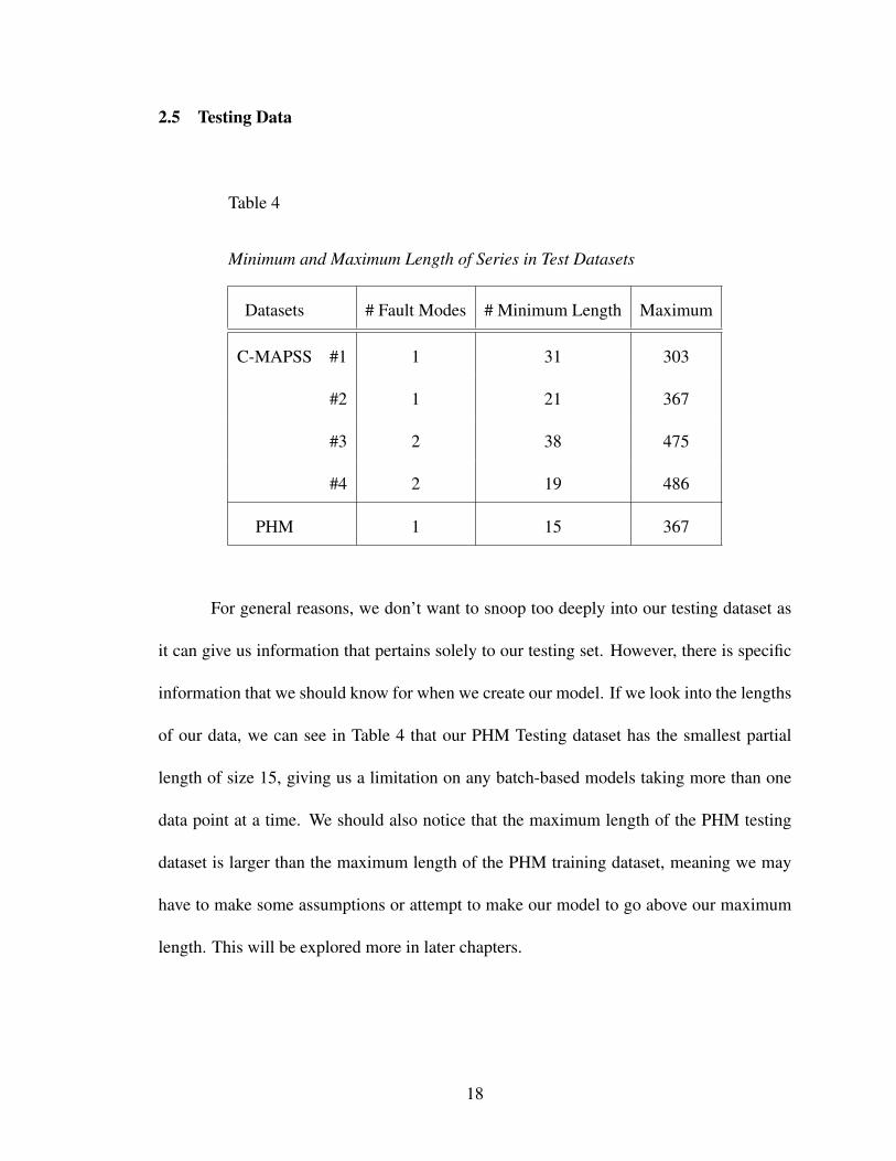
2.5 Testing Data

Table 4

Minimum and Maximum Length of Series in Test Datasets

Datasets # Fault Modes # Minimum Length Maximum

C-MAPSS #1 1 31 303

#2 1 21 367

#3 2 38 475

#4 2 19 486

PHM 1 15 367

For general reasons, we don’t want to snoop too deeply into our testing dataset as

it can give us information that pertains solely to our testing set. However, there is specific

information that we should know for when we create our model. If we look into the lengths

of our data, we can see in Table 4 that our PHM Testing dataset has the smallest partial

length of size 15, giving us a limitation on any batch-based models taking more than one

data point at a time. We should also notice that the maximum length of the PHM testing

dataset is larger than the maximum length of the PHM training dataset, meaning we may

have to make some assumptions or attempt to make our model to go above our maximum

length. This will be explored more in later chapters.

18

2.6 Experiment Layout

We will be doing several experiments focusing on the improvement of our score for

the PHM testing dataset, primarily through data preprocessing and post-processing. Each

experiment focuses on a specific method defined in chapter 3, how it improved our PHM

testing score, and a comparison to current methods used. These experiments are:

1. Scaled Target Function: Instead of using our basic target function or common alter-

native, we propose that scaling our target by some multiplier for training will give us

a better score.

2. Cycle Number Inclusion: The cycle number in each data point is commonly excluded

in many models. We believe that the inclusion of this cycle number will greatly

improve our score since it acts as a referential point of time for each data point.

3. Developing a Classifier Model: Classifications of healthy and unhealthy data points

has been discussed and developed in previous papers, but hasn’t been commonly used

in practice. We believe that a possible model could be made using these classifiers to

estimate the RUL.

4. Regime Partitioning versus Expanded Normalization: Two common approaches to

data preprocessing is regime partitioning and expanded normalization (standardiza-

tion). We would like to compare the results for each form of data preprocessing in

order to observe their strengths and weaknesses.

5. The Effectiveness of Aggregation and Filtering: Aggregation techniques have been

19

used successfully with neural network ensembles, primarily the use of Kalman Fil-

ters. We wish to implement and reproduce this success using alternative methods,

such as other models, curve fitting, and other filters and compare our results with

previously used filters.

By doing these experiments, we will be able to have a better understanding on our data

and how well different techniques can adjust our data to improve our model for estimation.

Each of these experiments also has a focused hypothesis, a defined methodology for how

we conducted the experiment, and the result that gives us insight and compares the results

or scores of other models.

2.6.1 Model layout. We must also have an understanding of what models we are

using in order to better comprehend our expected output and for the replication of our ex-

periments. We primarily focused on the use of feedforward neural networks (FNN), also

known as a multi-layer perceptron (MLP). Our secondary model used in some experiments

was a support vector machine (SVM) as well as other baseline models defined in our exper-

imentation.

We also used a validation set consisting of a portion of our training set (30% test-

ing/70% training split) to check for over-fitting of our training set. Our final model for

submission used all of our data from training. We can see the specifics for our FNN listed

below.

(a) Gradient Descent Optimizer: We primarily used Mini-Batch Stochastic Gradient De-

scent with a batch-size of 10 and at most 200 epochs. An Adam optimizer can be used,

normally with an epoch of about 80 without over-fitting.

20

(b) Activation Function: Our final model uses an ReLU activation function [11], but ear-

lier models experimented with logistic regression activation functions such as sigmoid

(σ(x) = 11−e−x ) and tanh(x). These are defined in our experimentation.

(c) Loss Function: We chose to use Mean-Squared Error (MSE) as our loss function.

(d) Layer Dimensions: Generally, each layer size was the same size, default size being 13,

with the output being 1. We generally used 1-2 layers for each network as the addition

of a third layer didn’t seem to improve results.

(e) Specialized Layers: We attempted to use specialized layers such as Dropout [12],

which thinned neural network layers by randomly deciding which nodes in a layer

to not use during training. Although this did improve some our of basic models, it

didn’t seem to improve later models being used.

For our SVM, the parameters are defined with each experiment, with exception to

our SMO SVM which is generated via Matlab and uses a Box Constraint array for our

soft-margin.

21

Chapter 3

Data and Target Function Processing

Although we may have an understanding our dataset, it would be improper to simply

plug in our data into any given model without processing it. As is typical in data analytics,

the processing technique used depends on the data. We can focus our preprocessing on

specific data columns, such as specific sensors, operating settings, or cycle number. This

also includes higher-level properties that are defined by our data such as the operating

conditions and fault modes. We may also post-process our resulting output from our model

in order to better remove any noise or to correlate the previous input to the current input of

the series. We may also find that different target function from the advised target function

could lead to better results or improved training of our model.

In this section, we will be discussing methods for processing our datasets as well

as their possible advantages and disadvantages compared to other methods. These methods

will then be used in each of our different models to evaluate their performance.

3.1 Overview

Broadly speaking, there are five categories of processing methods.

1. Basic normalization: These basic forms of preprocessing are commonly used in var-

ious forms of data and is not necessarily pertaining to our data. This includes scaling

our data, denoising, and standardization.

2. Regime partitioning: Modifications between datasets such as the number of operating

conditions and fault modes can greatly affect the performance for specific dataset

22

models, especially as they become more complex. We may see better performance if

we tried simplifying these properties by adjusting our data.

3. Data Selection: It is common to ignore some variables in a data vector in order to

remove unnecessary noise, processing of our model, or to simplify our series. These

choices are obviously dependent on the developer, as they can choose to remove spe-

cific sensors in each unit depending on its purpose and general display of usefulness

in modeling.

4. Filtering/Aggregating: Within all of our datasets, there is some form of noise that

exists, making it more difficult for us to pinpoint the exact RUL for a given data point.

This is also true for our output from most of our given models. A simple solution

for this would be to aggregate or filter either our input before training our model, our

model’s output before submission, or both.

5. Target function transformations: Instead of using our target function defined in sec-

tion 2.2, we may manipulation our target function to receive a better performance

from our model.

It is common for most developers to choose between some form of basic normal-

ization and regime partitioning; it is also typical to remove specific data that may or may

not benefit our data. We will be focusing on the specific details and differences used by

developers and study how they will perform. There has also been brief discussion of using

dimension reduction on our data which will be explored in later chapters.

23

3.2 Basic Normalization

When using any dataset, we are able to do basic transformations on our data points

using general knowledge of our training set. These techniques, although simplistic, helps

us expand to data outside of our training set and help better fit our data so that our model

may understand it. This adjustment of values in our data is commonly referred to as nor-

malization.

When normalizing, it is common to put our data in a normal distribution based on

our known dataset. This is useful as it not only centers our data to our origin, but also

treats each our data points equally. This can be done through a process called standardiza-

tion, where any data matrix X can be computed to the normalized X ′ using the following

equation:

X ′ =X−µ

σ

Where µ is the mean

and σ is the standard deviation

Figure 12. Standardization

However, standardization doesn’t set a distinct minimum and maximum between

all of our points. Instead, it simply scales down our data based on all of our values. It may

be important to set a strong minimum and maximum for our data in order to better fit a

model. Common examples are ranges of [0,1] and [−1,1] which a model can use to either

24

set stronger thresholds or to keep a consistent range between all values. This bounding

of data between a minimum and maximum is commonly known as feature scaling and is

computed as follows:

X ′ =X−Xmin

Xmax−Xmin

Where Xmin is the global minimum

and Xmax is the global maximum

Figure 13. Feature Scaling

When using these formulas on our function, we can immediately see an issue with

each of our data values as our sensors and operating conditions are expressed in different

magnitudes, as shown in Figure 16. This means our global data features (mean, standard

deviation, minimum, and maximum) might not properly represent each sensor.

To better incorporate this, we may instead obtain the global data features for each

corresponding column to obtain a data feature vector that can be used to normalize each

column. This is shown in Figure 14 and Figure 15, where f is the given column vector.

X ′( f ) =X ( f )−µ( f )

σ ( f )

Figure 14. Expanded Standardization

X ′( f ) =X ( f )−X ( f )

min

X ( f )max−X ( f )

min

Figure 15. Expanded Feature Scaling

25

(a) (b) (c)

Figure 16. Normalization Comparison(a) Original (b) Standardization (c) Feature Scaling

As we can see in Figure 17 and Figure 18, our data is much easier to understand and

has a stronger correlation between different sensors, removing the margins giving larger

separations between our sensors.

Figure 17. Expanded NormalC-MAPSS 1

Figure 18. Expanded ScaledC-MAPSS 1 [-1, 1]

3.3 Regime Partitioning

The basic forms of normalization work well for simple datasets such as C-MAPSS

1 and 3, but when we attempt the same transformation on PHM we can see a much noisier

plot being formed, as shown in Figure 19. As discussed in chapter 2, these unusual data

columns are formed by the operating conditions predefined in each dataset. These operating

26

conditions transform our dataset, making our sensors jump between different operating

conditions.

Figure 19. Original PHM Train

As discussed, these operating conditions can be generated using numerous methods

that shows the actual linear or exponential patterns shown within each of our sensors. For

our purposes, we will be generating the operating condition clusters using the 3 operating

settings discussed in chapter 2 and shown in Figure 11. For the purpose of this paper, we

will be referring to these operating condition clusters as regimes.

27

Figure 20. PHM Train Operating Conditions

The operating conditions is shown in Figure 20, but now with cluster centers defined

by using K-Means. These centers allow us to classify each point as a separate index from [0,

5]. Using this, we can expand on our previous, expanded normalization process. Instead

of simply normalizing each data column, we can instead split each data vector based on

our cluster classification, c, and then normalize each column in each cluster separately. By

doing this, our operating conditions will be centered, giving us a relation similar to a single

operating condition dataset. This process, also knonw as regime partitioning, is generalized

for standardization and feature scaling in Figure 21 and Figure 22 respectively.

X ′(c, f ) =X (c, f )−µ(c, f )

σ (c, f )

Figure 21. Regime-PartitionedStandardization

X ′(c, f ) =X (c, f )−X (c, f )

min

X (c, f )max −X (c, f )

min

Figure 22. Regime-PartitionedFeature Scaling

28

After using regime partitioning, we can see a vast improvement with our results.

Specific sensors seen in an dataset with 6 operating conditions, such as our PHM dataset,

resemble more of a simpler dataset with one operating condition, such as C-MAPSS 1. This

can be seen in Figure 17 and Figure 23. However, some sensors seem to be more useful

than others, having sensors with less prominent features or curves that better expresses the

deterioration of our engine. Please refer to section 3.4 for more details.

Figure 23. Regime-PartitionedNormal PHM Train

Figure 24. Regime-PartitionedScaled PHM Train

3.3.1 Clustering. When we know the number of operational conditions, it is easy

for us to cluster these operational conditions and perform regime partitioning. The separa-

tion can be done in numerous ways, as explained in section 2.4, using multiple signals, our

operating settings, Principal Component Analysis, as well as methods of manifold learn-

ing. Once we’ve done this processing, we can cluster our data using K-Means, K-Nearest

Neighbor, or some other methods when the number of clusters is known. From this we can

proceed this form of normalization.

However, it can become more difficult when the number of operating conditions

isn’t known, making this method impractical [10]. An easy solution for this is to change

the clustering method that can identify some unknown number of clusters. A simple method

29

for doing this is by using Affinity Propagation [13], which generates clusters by sending

messages between pairs of point until it converges. It also uses a damping factor, λ ∈

[0.5,1) that modifies each iteration by multiplying λ and adding 1−λ .

From doing a small number of experiments using our datasets, we found a damping

factor of 0.9 to be effective for finding the correct number of clusters for C-MAPSS 2, 4,

and PHM. However, it is more difficult to find the correct number of clusters for C-MAPSS

1 and 3, which have only one cluster. To solve this, you may incrementing the damping

factor via magnitudes (increment by 0.1 til fail, increment by 0.01 til fail, etc.) for a set

number of iterations. If you find that each iteration of using affinity propagation slowly

lowers the number of defined clusers, or there is no set number of clusters for n iterations,

then it is expected to be a single cluster.

We didn’t perform any major experiments on this methodology as it wasn’t the

focus of our research, but we found it to be effective with our pre-defined datasets. More

experimentation should with a variety of operating conditions and fault modes to ensure

effectiveness.

3.3.2 Purpose. The generalization of regime partitioning was discussed by T.

Wang [6], and has been used for several different models, such as MLP ensembles [1] and

expanding on Wang’s original works with trajectory-based similarity prediction [10]. It

is commonly used for simplifying our model, as seen with our comparison of Figure 17,

Figure 23, and our expanded normalized PHM sensors in Figure 19.

However, his method of normalization is mainly viewed in the simplification of

individual models and not much has been studied about the transferability of this method

to other datasets. We explore this in our experimentation and results.

30

(a) (b) (c)

Figure 25. PHM Train - Unit 1 Sensors(a) Upwards {2,3,4,8,11,13,15,18} (b) Downwards {7,12,20,21} (c) Shifting {9,14}

3.3.3 Issues. Some issues with using this approach is that some data columns be-

come unusable due to nil values. This includes our operating settings, which are constants

in each cluster. Because of the effects of standardization, each cluster is centered, mak-

ing each constant 0, and then divided by the standard deviation which is also 0. This also

occurs with sensors 5, 22, and 23, making them unusable for most situations.

3.4 Data Selection

As we saw in Figure 23 and Figure 24, there are sensors that don’t seem as important

as others, giving us less information and possibly effecting our model in a negative manner.

For these cases, it is often important to remove these weak sensors or focus on the stronger

features for each of these units.

From our observations of the regime-partitioned PHM dataset shown in Figure 25,

we can see interesting trends form in different sensors, usually going upwards, downwards,

or either in the case of Figure 25(c). More examples from other units validates these find-

ings, as well as observations of our C-MAPSS 1 dataset shown in Figure 26.

This analysis has also been done by in other studies, focusing instead on seven

31

(a) (b) (c)

Figure 26. C-MAPSS 1 Train - Unit 1 Sensors(a) Upwards {2,3,4,8,11,13,15,18} (b) Downwards {7,12,20,21} (c) Shifting {9,14}

sensors (2, 3, 4, 7, 11, 12, 15) instead of these groupings that we’ve discussed [2, 5]. A

possible reason for choosing these seven is to avoid the splitting that is seen in Figure 25(a)

with sensors 8 and 13, and also to focus more on sensors that are more continuously giving

us clean results.

Another commonly avoided column for each of our data vectors are the unit number

and cycle number defined for each unit. Although the unit number should be avoided

since the engines are defined anonymously (as in unit numbers can be swapped without

consequence), our cycle number is a set point of time for each data point and cannot be

swapped between data points within our dataset, or within individual series. The cycle

number is normally substituted in for comparing larger sets of the series, such as the use

of recurrent neural networks or similarity-based approaches, but we wish to use the cycle

number directly in order to have our model have a more direct component of time.

3.5 Filtering and Aggregation

We can see in Figure 25(b) that there is some amount of noise in each of our sensors.

In practice, this is also true for the output of our model when input said noisy data, resulting

32

in a noisy output. A simple fix for this the use of a filter that can adjust our sensors or output

for said noise, giving us a cleaner result. This has been described thoroughly in several

different papers [1, 6, 9], but we would like to view the different filters that are commonly

used and what we believe are also excellent filters for this problem.

3.5.1 Regression. An obvious choice would to simply fit a line or non-linear

curve onto our given signal. For sensor data, a well fitting curve would be an exponential

curve [6] based on the following equation:

z = a∗ eb∗t + c

where a, b, and c are the learned parameters, t is the index (or cycle number), and z is our

new output fitted to the sensor input x of index t.

For outputted data that is based on our linear target, we suggest using a 3rd order

polynomial curve defined as:

z = a∗ t3 +b∗ t2 + c∗ t +d

where a, b, c, and d are learned parameters. This can clearly vary depending on models,

but we found it to be a good fit for our defined models and should cover outputs similar

to what was shown by Heimes [3]. In this case, z is the new output for the original RUL

output of a model.

However, this only works when give the full or a large percent of data for a given

unit, making this inefficient when given small, partial series such as what is used in our

33

testing series. For these cases, we would suggest using a linear model defined as:

z = a∗ t +b

This linear regression acts similar to our previous two regression models. For our experi-

ments, we use this linear model when the length of the series is less than 30.

The use of fitted regression algorithms gives us a perfectly smooth output, which

can be a problem for if we assume too much of our data is noise. For this reason, the use

of actual filters may give better performances, keeping more of our noise in order to keep

more of our actual data.

3.5.2 Kalman filters. A filter that is commonly used in not only this problem

[1, 6] as well as several others is the Kalman Filter. Several different Kalman Filters have

been used with great success, but also with large amount of variance. To avoid focusing

on a single class of filters, we decided to make a simple Kalman filter based on Welch and

Bishop’s introductory paper [14].

3.5.3 Butterworth filter. The Butterworth filter is a relatively simple, but effec-

tive filter that uses two coefficients in a forward-backward filter [15]. This gives us a very

smooth output after filtering similar to our Kalman filter. However, we do see more curves

near the end of some partial series, giving a possible over-estimation of our data. To avoid

this, we change the order for our butterworth coefficients from 3 to 1 when the length is

less than 30, similar to our regression models.

3.5.4 Savitzky-Golay filter. Many of our previous filters focuses on giving us a

fairly smooth output after filter. However, focusing on smoothing the connections from one

34

point to another leads to possible over-curving of data and a poor estimation. Furthermore,

a focus on our entire, noisy se ries can lead to other poor estimations. For this reason,

the Savitzky-Golay filter is an excellent alternative to our previously defined filters [16].

Unlike many of our other filters, it focuses on a ”window” of adjacent points and fits it

to a low-degree polynomial. For our experiments, these windows would use a third of the

total length of the series, but would be capped at 33 if they were too large. Similar to our

regressions models and butterworth, our order was set to 3 if the length was greater than

30, else it was set to 1.

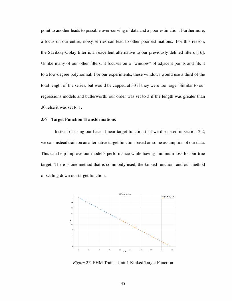
3.6 Target Function Transformations

Instead of using our basic, linear target function that we discussed in section 2.2,

we can instead train on an alternative target function based on some assumption of our data.

This can help improve our model’s performance while having minimum loss for our true

target. There is one method that is commonly used, the kinked function, and our method

of scaling down our target function.

Figure 27. PHM Train - Unit 1 Kinked Target Function

35

Kink(x) =

130 if x≥ 130

x otherwise

Where x is the computed RUL for a training unit.

Figure 28. Kinked Equation

3.6.1 Kinked function. The kinked function is a commonly used target function

defined originally developed by Heimes for the original 2008 competition [3], and has been

used to improve more recent methods as well [1]. It originates from the idea that the lowest

run length is 128 (127 if starting at 0), and having the later, unhealthy portions of our series

defining the actual RUL. This means we can instead focus less on the healthier portions of

our series and focus more on the later, more defining features.

By taking this into account, we can define a target function take has our RUL de-

fined as 130 if our linear RUL is normally greater than or equal to 130, and is otherwise the

linear function itself. This is visualized in Figure 27 and is formalized as:

However, this function may over-assume parts of our testing set which only contains

healthy states. For instance, in our PHM testing dataset, we have a unit that is of length

15. Because all of our series start healthy, we know that a good portion of these data points

might be healthy and default to 130, giving a possible worse estimate.

3.6.2 Scaled target function. Instead of adding a kink to our target function, we

can instead keep our target linear, but scale down our targeted output instead. This can be

done by looking at the maximum RUL of our given dataset and dividing our original RUL

36

by that maximum, giving us a scale from 0 to 1. This is typically done for converting our

regression model of [0,∞] to a logistic regression model of [0,1]. After training, we can

input our testing dataset to our model and multiply by the maximum RUL, also referred to

as the max-multiplier of our model. Doing this may help in simplify our learning and also

make a clearer assumption about the expected length for a dataset.

Figure 29. PHM Train - Unit 1 Scaled Target Function

This can also be expanded to scaling our model from [−1,1] by then multiplying

our [0,1] target by 2 and subtracting by one. Any expansion can be described using the

feature scaling algorithm. For our purposes, we will be focusing on simply scaling down

our target function to [0,1]. This can be seen in Figure 29 which scaled the first unit of our

PHM training dataset by the max RUL, 356.

37

Chapter 4

Experiments

We can see from chapter 3 that there different methods of preprocessing and post-

processing data, as well as the different available target function for our model to train on.

To further understand these methods require a breadth-first search for us to see their general

effectiveness, as well decided on more general methods and combinations of methods in

order to optimize our results. This is reflective of our experiments, defined in section 2.6. In

this chapter, we are showing our hypothesis, methodology, and results for each experiment

as we approach a better model.

As previously stated in chapter 1, we have a score function (Figure 1) that increases

as when RUL estimation is over or under the exact amount. The score function also gives

a heavier penalty for over-estimations than under-estimations. For instance, an overestima-

tion of 60 leads to a score increase greater than 400, while an underestimation of 60 leads

to a score increase of approximately 100.

4.1 Baseline Models

Early on we chose to use feedforward neural networks (FNNs) due to familiarity

and existing libraries that heavily support it (primarily Tensorflow and Torch). In order to

confirm our results with our FNN model, we decided to create several baselines for when

we heavily modify our FNN model. We preprocessed our data using expanded standard-

ization, a very simple form of preprocessing that would keep our data in a simple range.

Using this, we generated several different models with a basic target function and used this

as our starting baseline. The score would be based on our submitted PHM testing dataset.

38

Table 5

Baseline Models Comparisons

Model PHM TEST Score

Linear SVM 23,509.33

SMO SVM 24,060.66

Ensemble 482,740.00

Gaussian 2,363,057.25

Decision Tree 1,288,502,988.08

4.1.1 Results. From these results in Table 5, we get an understanding that the

linear model is the best model followed by our SMO SVM, and our other models are fairly

weak. This could also be due to the difficulty of the problem, where our linear model is

performing the best based on its simplicity. If we were to submit an RUL of 54 for all

218 units in our PHM testing dataset, we would find this aligns with this conclusion as this

constant gives us a score of 24,505.19, only slightly worse than our SMO SVM.

We can take 2 major points from these results:

1. Our model should be relatively simple to achieve better results.

2. Scores of 20,000 or greater are weak predictors.

The first point is fairly obvious and follows Occam’s razor. However, the second point

tells us what models gives us an insight to the unit series and what models tell us little or

nothing. We may possibly assume that the average of this constant RUL score may give us

39

insight to other datasets as well for comparing results (24,505.19218 = 112.41).

4.2 Max-Multiplier Experiment

The use of FNNs is fairly common for this problem and has been done several times

using the basic target function. The kinked function was also defined in several papers and

in practice [1], leaving us to more thoroughly investigate the idea of scaling the target

function using a multiplier.

4.2.1 Hypothesis. We didn’t believe that this form of optimization would lead to

any absolute failures and believed that, at worst, it could slightly lower the score of good

models. For this reason we wanted to focus on creating what we considered the best model

using this method and compare to see whether it actually improved our model.

As for actual improvements, our hypothesis is that scaling down our data would

improve our model results and aid in the training of our model, or at worst do nothing to

our data. We will be focusing more on this hypothesis in our comparison.

4.2.2 Methodology. We used an initial FNN (24x5x3x1) similar to what was

described by Heimes [3]. If you notice, we are only taking 24 inputs, meaning we are

excluding our cycle number and unit number from our input. Our initial activation function

were sigmoids (σ(x) = 11+e−x ) since our data was scaled from 0 to 1, making our neural

network estimator for the RUL take a logistic regression approach. We then attempted to

scale up this model in order to achieve better results.

40

Table 6

Initial Neural Network Comparisons


24x5x3x1 47,457.67

24x13x13x1 31,746.61

24x13x13x1 w/ 1st Layer Dropout 18,892.87

4.2.3 Results. Initially, our neural network did incredibly poorly, scoring worse

than our linear model and our constant RUL. We then tried to improve our model using

adding another hidden layer, which improved our score by over 10,000, giving us a new

score of 31,746.61. However, we shouldn’t consider this a victory since it is still worse

than our baseline score. The biggest improvement was the use of Dropout [12] with a 50%

probability of cutting an output from our first layer. By adding this one change our score

was cut by almost half, and more importantly, putting us below our baseline.

We can also compare the results of our first and second best models from Table 6

by graphing a unit series from a validation set. If we observe Figure 30 and Figure 31, we

see our Dropout model, which performs better than our non-Dropout model, has a larger

amount of noise generally seen with each unit in our validation set. We would expect the

opposite to occur based on our scores, but based on the figures we assume visualizations of

these output are inaccurate, at least until we achieve better results.

41

Figure 30. PHM Train Validation Set(24x13x13x1)

Figure 31. PHM Train Validation Set(24x13x13x1 - Dropout)

After running these models we attempted to improve our model using similar meth-

ods, but with no success. This concluded our experimentation with our max-multiplier, as

we decided to focus on other experiments.

4.3 Cycle Number Inclusion Experiment

Currently, most models exclude the cycle number of a given data point to instead

use some form of aggregation or continuation such as recurrent neural networks to chain

data points together. Instead, we chose to keep our model simple by using our basic FNN

and including this cycle number as part of our data.

4.3.1 Hypothesis. Our hypothesis is that the inclusion of the cycle number will

improve the results dramatically as well as improving our structure of our output. This

belief comes from how our RUL itself comes from our cycle number and giving our models

a comparative stance between different data points.

4.3.2 Methodology. To show this, we generated two similar models based on our

current best model defined in Table 6. In this case, we use the same model with 24 inputs

and another model with 25 inputs. We also updated our activation function to use ReLU

42

[11] for easier experimentation with later examples. This change of activation function still

keeps our score relatively the same.

Table 7

Cycle Number Inclusion vs. Exclusion


Without Cycle Number 18,892.87

With Cycle Number 9,946.4

4.3.3 Results. We found the results after using the cycle number to be staggering.

Once again, our score has been cut in half, giving us a much better model for us to work

with. Another staggering result comes from removing the Dropout layer, cutting our score

by more than a third with a result of 3,285.91. Because of this, our best model removes

Dropout, giving us a 25x13x13x1 FNN with ReLU activation functions.

When comparing this current model with other scores, we found that it outper-

formed methods using the basic linear target function and kink target function [1]. We

were also able to replicate these scores for each target function and found our reasoning to

be sound.

4.4 Classifiers Exploration

We decided to attempt another approach in estimating the RUL for each series based

on other methods. In Heimes’ paper [3] he experimented with a basic classifier, classifying

the first 30 of each unit in our PHM training set as healthy and the last 30 as unhealthy.

43

Using this data, he found it was easy to train a basic FNN model.

Figure 32. Accurate PHM Train UnitFNN Classifier

Figure 33. Inaccurate PHM Train UnitFNN Classifier

When replicating, we found it to be fairly accurate, but with some issues with our

validation set. This can be seen in Figure 32 and Figure 33. The use of an SVM Classifier

can improve this, but assumes our data is absolute 0 and 1, as shown in Figure 34 and

Figure 35.

Figure 34. Accurate PHM Train Unit(100% Accuracy) SVC

Figure 35. Inaccurate PHM Train UnitSVC

However, when using our models to predict the PHM testing dataset we found that it

didn’t seem to make any accurate predictions, as shown in Figure 36. We then built similar

44

models, but using the cycle number as an additional input. By doing this, we saw clear

patterns of transitions from 0 (healthy) to 1 (unhealthy) in larger test series. This trend is

shown in Figure 37. Although we can’t make an accurate score because of this being our

test set, we can believe that the inclusion of this cycle number improved our results due to

the expected trend.

Figure 36. PHM Test UnitFNN - No Cycle

Figure 37. PHM Test UnitFNN - Cycle

4.4.1 Hypothesis. Using these classifiers, we may create a new way of generating

the RUL estimation for each PHM test series. Our hope is that this method will achieve

better results than our aforementioned score of 3,000.

4.4.2 Methodology. Our first thought was to split our data further instead of

simply using the first and last 30 for each series. To do this, we took each series and split

them into 5 buckets containing 20% of the series. We then generated 4 classifiers, each

splitting the buckets so that N buckets represent the data points below (N * 20)% of the

series, classified the 0. The rest are then classified as 1, representing being above our split

point. Each model would consist of either the use of SVC or a FNN that consisting of the

same hyper-parameters defined with our results.

45

After generating each classifier, we then split our classification by taking a average

of a window throughout the series until we reach an average ≥ 0.5, in this case we chose

a window size of 5. We also experimented with how to exclude specific classifiers if given

faulty results, such as be given a series size less than the percentage rated by the classifier.

4.4.3 Results. As shown in Table 8, an initial use of an SVM finds our results to

be poor, doing worse than our linear model and our constant RUL model. We attempted to

remedy this by changing the soft-margin for the SVM, and found a middle ground of 100

gave us the best results. However, this didn’t line up with our scores for our validation set

that found lower penalties gave better results.

Table 8

SVC Classifier Comparison

Models Test Score Notes

SVC(C=1, degree=3) 22,041,035.27 If RUL < 0, negate



SVC(C=50, degree=3) 761,054.59 If RUL < 0, negate

SVC(C=100, degree=3) 759,380.40 If RUL < 0, negate



We then changed our model to an FNN using ReLU activation functions and found

46

our results drastically improved, but not enough to beat our linear model. We also tried to

increase the size of our model, which did give us improvements but, we found that our best

score was still 10 times more than our baseline models.

Table 9

FNN Classifier Comparison

Models Test Score Notes

MLPClassifier((32, 24, 16)) 525,979.31 results ≤ 0 become 0

MLPClassifier((32, 24, 16)) 297,137.01 results ≤ 0 are ignored

MLPClassifier((32, 24, 16)) 391,050.62 results ≤ 0 are ignored

MLPClassifier((32, 24, 16)) 248,462.45 If output is < 0, negate

We also ran into issues with negations and models classifying the entire partial

series the same, making our ensemble more difficult to deal with. We found the best way

was to negate these values, which still gave us several issues to deal with. In short, we

couldn’t find an effective way to use this ensemble.

4.5 Regime Partitioning

After running with expanded normalization, we decided to attempt to improve our

model using regime partitioning as our main method for preprocessing. We wanted to

attempt to see the advantages to regime partitioning to our current method and if there was

any actual advantage for the PHM dataset alone.

After working our experiments with our PHM dataset, we decided to expand our

47

work to the C-MAPSS dataset to see how our methodologies compare with different, but

similar datasets. Although our previous results are valid for PHM, harder datasets may

become more difficult to deal with or less complex datasets are easier to deal with. This

seems to hold true for other papers that analyzes more than just PHM [1, 10]

4.5.1 Hypothesis. We expect regime partitioning to improve the results for our

model and making it more relatable to other datasets by simplifying the clustering used for

operating conditions.

4.5.2 Methodology. We will be using a (25x13x1) model with ReLU activation

functions for our expanded normalization and a (19x13x1) model with ReLU activation

functions for our regime partitioning. This lowering of inputs is due to the operating set-

tings becoming nil after performing regime partitioning and some nil sensors as well.

We also expanded these experiments for other datasets as well and for models with-

out the use of cycles. We hope that this will give us more insight into the performance of

other datasets and how well they fit into our current best model.

Table 10

Expanded Normalization vs Regime Partitioning

Preprocessing Method PHM Test Score

Expanded Normalization 3788.18

Regime Partitioning 7454.48

48

4.5.3 Results. We can see in Table 10 that our hypothesis was wrong for the PHM

dataset. Our expanded normalization preprocessing outperforms our regime partitioning

method. This is incredibly odd since most people tend to use regime partitioning in some

form for the preprocessing [1, 6, 10]. We also confirmed by improving our model, receiving

similar results to the first place winner [5].

We should expect regime partitioning to have some advantage over different datasets,

especially considering how it reduces the operating conditions for all datasets. For this rea-

son, we decided to continue experimenting using several datasets instead. We also focused

on submitting to each testing dataset for each of our datasets in order to see any transfer-

ability that could possibly exist.

Comparing Table 11 and Table 12 shows an unusual side that we didn’t notice

before. Although our cycle number does improve each of our datasets in comparison of not

using a cycle number, we find that training on other datasets, in some cases, gives us better

performances. This can be seen with training on C-MAPSS 4 and testing on C-MAPSS 2,

and larger effect can be seen when training on C-MAPSS 1 and testing on C-MAPSS 3.

49

Table 11

Total RUL Score (Expanded Normalization w/ Cycle Number)

C-MAPSS 1 2 3 4 PHM

(100 Units) (259) (100) (248) (218)

3429.553159 2399917.454 22300.42896 1647158.566 180336.68

4.05867E+23 44638.41142 5.09041E+27 49295.23293 624058.5

68866916.31 3.20382E+17 611805096.2 9.71451E+15 1.24402E+15

3.71893E+34 34429.74452 7.57986E+43 50885.48583 2.85E+12

7.29278E+24 4.84E+13 8.35206E+24 1.02901E+15 3788.18

Best Average Scores Per Unit

34.29553159 132.9333765 223.0042896 198.7711005 17.37697248

50

Table 12

Total RUL Score (Expanded Normalization w/o Cycle Number)

C-MAPSS 1 2 3 4 PHM

(100 Units) (259) (100) (248) (218)

3803.443683 14824498464 28085.71268 12252365456 305838154026

7.94307E+60 37548.80635 5.74752E+48 273777.7273 15241257.85

84630.96189 5.67E+14 1799097270 4.00E+14 2.73E+16

1.68878E+47 141227.5593 1.29892E+57 125751.2301 7.99E+20

6.84274E+25 4.10664E+17 4.28921E+23 3.99788E+17 19028.79883


38.03443683 144.9760863 280.8571268 507.0614119 87.28806802

We also find that PHM is the best performing out of all of these methods, followed

by C-MAPSS 1, which has double the average score. Training on more complex model

improves C-MAPSS 1 down to an average score of 27.20, but this still doesn’t beat our

PHM test dataset score.

51

Table 13

Total RUL Score (Regime Partitioning w/ Cycle Number)

C-MAPSS 1 2 3 4 PHM

(100 Units) (259) (100) (248) (218)

3020.925557 168353.4269 640517.8762 11605879.04 9953.780619

4291.80613 43024.96287 6918.228081 85679.14248 6583.142585

33698.13 626170681 1400206201 96972108.7 3975518.175

32251.86555 903563.2456 6734.379265 136110.2005 219623.6999

4121.551745 36958.98043 4343.471254 37361.1906 7454.484125


30.20925557 142.6987662 43.43471254 150.6499621 30.19790176

52

Table 14

Total RUL Score (Regime Partitioning w/o Cycle Number)

C-MAPSS 1 2 3 4 PHM

(100 Units) (259) (100) (248) (218)

3795.738041 2351129.624 6011.477993 882622.7645 144126.4734

6575.075802 43700.05936 14441.78701 255942.8523 22050.56435

187766.8253 45561902395 339487646.4 11410625871 6642300.283

5768461.887 1086365.845 36355.79442 171475.16 452604.8415

4937.49241 39277.00515 21200.11688 337992.5004 70942.42205


37.95738041 151.6486685 60.11477993 691.4320969 101.1493778

We found that using regime partitioning, the general results for 3 of our 4 C-MAPSS

datasets did improve, but still in strange ways. Our best method for training C-MAPSS 3

and C-MAPSS 4 datasets was by training our model on our PHM dataset. Oddly enough,

our C-MAPSS 2 dataset didn’t improve at all from this transition, as well as our PHM

dataset. However, C-MAPSS 1 improvement is self-contained and due to the decrease of

inputs.

We can also analyze the relation between these datasets, and although the score

didn’t improve for some datasets, we do see some score improvements based on relations,

as well as an lower total average between scores trained on different datasets. We also

53

see C-MAPSS 2 giving PHM a better output than training on PHM in this case, similar to

our previously described relations with other datasets. This makes regime partitioning a

possible improvement for more general datasets, especially when dealing with an engine

differing from our training set.

4.6 Aggregation via Filtering

We found our current best model gives us a score of 3285.91, but this can still be

better improved for PHM by using different techniques. In this case, we wish to improve

the noise of our current output model by using some method of filtering. This method of

filtering has been used before with specialized Kalman filters [1], but we wish to look at

simpler methods in order to see what types of filter may work better given specific circum-

stances.

4.6.1 Hypothesis. We believe filtering our output will improve the score of our

model by a significant amount, but different methods that could over-smooth our output

could cause damage to our score instead.

4.6.2 Methodology. We will be using the following methods for filtering the same

output for our best model (25x13x13x1 with ReLU activation functions):

1. SVM

2. Random Forest

3. Fitted Curve

4. Butterworth Filter

5. Savitzky-Golay Filter

54

Each method will then be compared with the original output and the other method used,

along with an analysis of their performance compared to their filter. We chose against using

the Kalman filter as it was previously done by Lim’s team with other specialized Kalman

filter that we didn’t focus on building due to time constraints. We will be comparing our

score difference with theirs as a result.

4.6.3 Results. The SVM and Random Forest models were trained by taking the

output of our best model as an input and re-training with our target function. Using this

method, both models failed in incredible fashion, possibly adding more noise to our output.

This can be seen in Figure 38 and Figure 39, which is shown adding more noise or having

no effect on our PHM testing dataset. In both cases, the models made our output worst,

giving us a score of 4549.81 and 18,558.33 for the SVM and Random Forest respectively.

Figure 38. PHM Test Unit 31SVM Filter

Figure 39. PHM Test Unit 31Random Forest Filter

However, using the fitted curve described in chapter 3, we can instead fit our out-

putted series to a 3rd order curve or 1st order line depending on length. Doing this removes

the chances of noise and helps us better filter our model. We can see relative success based

on the curved line in Figure 40 and Figure 41 that is based on our noisy output. These

55

figures also show that the polynomial is more centered throughout our noisy output instead

of estimating over or under, although there are some curves that go over specific periods of

our output series.

Figure 40. PHM Train Unit 1Polynomial

Figure 41. PHM Test Unit 31Polynomial

By using this polynomial as our new output, we found our results improved from

3285.91 to 2700.20, or a reduction of 17.82%. Although we find this method to be effective,

it is possible that we are over-simplifying our model. This can be seen in Figure 42, draws

a line within 15 data points. This new output might be overly-centered, as we don’t have

later data points that give us more information later on to drag our polynomial down. To

fix this, we can refer to our actual filters.

Our first filter, the butterworth filter, is a classic filter used for several problems

with signals. If we look at Figure 43 and Figure 44, we can see a similar pattern to our

polynomial curve fit, but with a better fit to local data. Because of this, we expect a better

score for our new output.

56

Figure 42. PHM Test Unit 150Polynomial

Figure 43. PHM Train Unit 1Butterworth

Figure 44. PHM Test Unit 31Butterworth

However, we instead find that our results slightly increased to 2739.74, still a major

reduction when compared to our PHM dataset. We found this odd, as it looks as if it

is better fitting with our data, as seen in Figure 45, however we do see some curving in

57

the beginning and end of some series, possibly leading to slight over-estimations or under-

estimations. Considering that we look at the last value of our series for the RUL estimation,

this can become a concern.

Figure 45. PHM Test Unit 150Butterworth

Many of these previous filters focus on smoothing, which could lead to some, local

oddities within our data. A simple way to this is to use a convolution-based filter with

a window so that it can focus solely on a local region instead of the entire data series at

whole. This convolution-based filter is also known as the Savitzky-Golay filter, and for

our version of this filter we have not only lowered the polynomial order for shorter, partial

series, but also varied the window size based on length as well (more details in chapter 3).

58

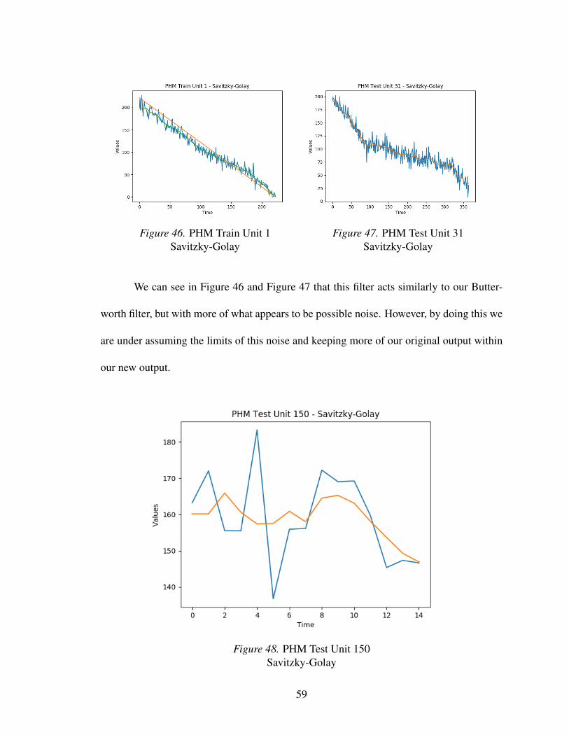
Figure 46. PHM Train Unit 1Savitzky-Golay

Figure 47. PHM Test Unit 31Savitzky-Golay

We can see in Figure 46 and Figure 47 that this filter acts similarly to our Butter-

worth filter, but with more of what appears to be possible noise. However, by doing this we

are under assuming the limits of this noise and keeping more of our original output within

our new output.

Figure 48. PHM Test Unit 150Savitzky-Golay

59

After submitting the output result of this filter, we can see a tremendous amount of

success, as we a score of 2,260.69, reducing our original best model score of 3285.91 by

almost a third. We believe this is caused by the lack of assumptions as seen in other filters,

keeping some amount of noise in order to make sure no proper data is lost. We can see

in Figure 48, as our filter stays as the last value despite filtering, meaning no unnecessary

moves are made and our new output defaulted to the original output.

Table 15

Filter Comparison

Filter PHM Test Score Original Score Reduction %

Polynomial 2,700.20 3,285.91 17.82%

Butterworth 2,739.74 3,285.91 16.62%

Savitzky-Golay 2,260.69 3,285.91 31.20%

Kalman Filter Ensembles [1]

Kalman Filter (KF) Ensemble 5,590.03 6,103.46 8.41%

Switch KF Ensemble 2,922.33 6,103.46 52.12%

When comparing our filter’s performance with the performance of Lim’s Switching

Kalman Filter (SKF) Ensemble, we find that the SKF Ensemble out-performs our filters by

at least 20%. However, the jump performed by their filter began at 6,101.46, almost double

the size of our best model before aggregating. This could lead to worst performance with

ours or low-scoring model, as seen with other methods. However, more experimentation

60

must be done to confirm this new hypothesis.

61

Chapter 5

Conclusion

In the beginning of this thesis, we discussed the importance of RUL estimations

and how they are a modern problem in prognostics and engineering. We also discussed the

common methods used, such as similarity-based approaches [5, 6, 10], feedforward neural

networks and recurrent neural networks [3], as well as methods of improving feedforward

neural networks using filters [1]. We then focused on what our data is, what each data

feature and column represents, as well as our own models used for the experimentation.

We discussed the different methods used, their commonality, as well as how we

would use each method. Our experimentation showed the improvements of scaling our

target function, our failures in classification models, as well as focusing on the effectiveness

of regime partitioning versus the simpler, expanded normalization method. We would also

review aggregation, using our own filters and models as we compared their performances

with each other and other published methods used.

From these observations and writings, we believe we’ve successfully improved our

model with rigorous experimentation and focus, having a final score of 2260.69. We found

our model to out-perform other common models based on our research using different

methods that have been reproduced. This research can continue and expand to different

models and methods that can further improve our results, such as the use of transferable

datasets as more data. We hope that in the future this will act as a basic guideline and aid

in future performance of RUL estimation models. However, there are some ways that we

can better improve our model in the future as well as looking into more general models for

62

working with several datasets.

5.1 Future Work

From our experiments, we have explored different options for improving our data

and model for RUL estimations. This had us focus on a breadth-first search as we attempted

different methods both new and old in order to have a better understanding of the problem

in general. Although this led to our previously discussed experiments, we still have other

ideas, hypotheses, and implementations that we would wish to see fleshed out in the future.

5.1.1 Transferability of datasets. We previously showed that regime partitioning

doesn’t improve our score more than expanded normalization for the PHM dataset, but

it does allow a stronger transferability between datasets of different operating conditions

and fault modes. We wish to expand this topic on the transferability between datasets

within later research, using multiple datasets for training and ways to improve and detect

properties of models.

We have done this within our own research briefly, where training with C-MAPSS

2 and PHM has improved our score for our PHM training sets, for expanded normalized

data. However, we wish to continue this experimentation in hopes of combining more data

from different datasets will consistently improve our results. This would allow for more

data to be preprocessed and added to further improve our model, but also allow the creation

of an effective, generalized model for any dataset.

5.1.2 Searching for a better scaling multiplier. In our experiments, we consis-

tently used a scaled target function to improve our training. This scaled multiplier that we

used was the maximum RUL for the dataset, giving us a maximum of 1 and a minimum

63

of 0. Although this method was more effective than the kinked target function and basic

target function, we found an interesting pattern if we took this further.

Let us start with a multiplier of 1, making our target function the original, basic one

defined in chapter 2. We can train a model using this target function, score, and repeat with

an incremented multiplier. By doing this over and over, we find a pattern emerges where

a smaller score is found for a given multiplier. This score would also slowly increase in

correspondence with an increasing multiplier.

We can also see improvements from C-MAPSS 3 when using C-MAPSS 1, where

we can score C-MAPSS 3 lower than C-MAPSS 1 using the C-MAPSS 1 training set. This

is incredibly impressive especially when considering that C-MAPSS 3 is a more difficult

dataset than C-MAPSS 1. We may also see similar improvements between C-MAPSS 2

and C-MAPSS 4 as well.

However, we chose not to chose any of these results as we did this late within our

experimentation phase and used our testing dataset to show this instead of a separate vali-

dation set. We would rather use this separate validation set and include the PHM datasets

as it would further validate our methodology and prevent any form of snooping with our

testing datasets.

5.1.3 Incrementing our target function. As defined in the original PHM ’08

competition, our model should estimate the number of cycles after our current cycle. This

would mean our last cycle would have an RUL of 0, our second to last cycle being 1, and so

on [8]. However, when experimenting with our target function we found an improvement

with our results when increasing our basic RUL target function by 1 before scaling.

64

When using a 25x13x1 FNN model, we found that the original, scaled target func-

tion gave us a score of 3788.18, but when using our incremented, scaled target function we

found an improved score of 3439.87, an improvement by over 300 points. We also found

this to improve not only our PHM dataset, but all of our datasets. We are unsure whether

this means we are mostly under-estimating and doing this would work against going un-

derneath our curve, or whether it simply improves our model output’s structure somehow.

We are hoping to explore this effect more in the future and see whether we can search for a

better target function using these methods.

5.1.4 Preprocessed aggregation. In our experiments we used the inclusion of

the cycle number as a way to perceive time within our model. More than this parameter

being an extra column in each data point, it can also act as its own linear function for each

unit. When imagining the cycle number as a model instead of a piece of data we find more

possibilities emerge.

One that has been discussed before is the use of an exponential curve regression for

our input data, having major sensors be fitted to a curve for better clarity [6]. This might be

comparable to our experiments with post-processed aggregation and filter, where we used a

3rd order polynomial to fit our original output. We may attempt to generate our exponential

curve similarly to our post-processing polynomial as well as do similar experiments with

filtering algorithms in order to see how well our model performs with filtered inputs.

However, due to time constraints we were unable to perform any preprocessing

aggregation and filtering with our datasets, leaving this as something we hope to experiment

with in the future.

65

References

[1] P. Lim, C. K. Goh, K. C. Tan, and P. Dutta, “Estimation of remaining useful lifebased on switching kalman filter neural network ensemble,” in Ann. Conf. PrognosticsHealth Manag. Soc, pp. 1–8, 2014.

[2] E. Ramasso and A. Saxena, “Performance benchmarking and analysis of prognos-tic methods for cmapss datasets.,” International Journal of Prognostics and HealthManagement, vol. 5, no. 2, pp. 1–15, 2014.

[3] F. O. Heimes, “Recurrent neural networks for remaining useful life estimation,” inPrognostics and Health Management, 2008. PHM 2008. International Conferenceon, pp. 1–6, IEEE, 2008.

[4] E. Ramasso, “Investigating computational geometry for failure prognostics.,” Inter-national Journal of Prognostics and Health Management, vol. 5, no. 1, p. 005, 2014.

[5] T. Wang, J. Yu, D. Siegel, and J. Lee, “A similarity-based prognostics approach forremaining useful life estimation of engineered systems,” in Prognostics and HealthManagement, 2008. PHM 2008. International Conference on, pp. 1–6, IEEE, 2008.

[6] T. Wang, Trajectory similarity based prediction for remaining useful life estimation.PhD thesis, University of Cincinnati, 2010.

[7] L. Peel, “Data driven prognostics using a kalman filter ensemble of neural networkmodels,” in Prognostics and Health Management, 2008. PHM 2008. InternationalConference on, pp. 1–6, IEEE, 2008.

[8] A. Saxena and K. Goebel, “Phm08 challenge data set,” NASA Ames Prognostics DataRepository (http://ti. arc. nasa. gov/project/prognostic-data-repository), NASA AmesResearch Center, Moffett Field, CA (consulted 2014-02-15), 2008.

[9] A. Saxena, K. Goebel, D. Simon, and N. Eklund, “Damage propagation modeling foraircraft engine run-to-failure simulation,” in Prognostics and Health Management,2008. PHM 2008. International Conference on, pp. 1–9, IEEE, 2008.

[10] J. Lam, S. Sankararaman, and B. Stewart, “Enhanced trajectory based similarity pre-diction with uncertainty quantification,” PHM 2014, 2014.

[11] V. Nair and G. E. Hinton, “Rectified linear units improve restricted boltzmann ma-chines,” in Proceedings of the 27th international conference on machine learning(ICML-10), pp. 807–814, 2010.

[12] G. E. Hinton, N. Srivastava, A. Krizhevsky, I. Sutskever, and R. Salakhutdinov, “Im-proving neural networks by preventing co-adaptation of feature detectors,” CoRR,vol. abs/1207.0580, 2012.

66

[13] B. J. Frey and D. Dueck, “Clustering by passing messages between data points,” Sci-ence, vol. 315, no. 5814, pp. 972–976, 2007.

[14] G. Welch and G. Bishop, “An introduction to the kalman filter,” 1995 (Accessedin March 2017). https://www.cs.unc.edu/~welch/media/pdf/kalman_intro.pdf.

[15] S. Butterworth, “On the theory of filter amplifiers,” Wireless Engineer, vol. 7, no. 6,pp. 536–541, 1930.

[16] W. H. Press and S. A. Teukolsky, “Savitzky-golay smoothing filters,” Computers inPhysics, vol. 4, no. 6, pp. 669–672, 1990.

67

https://www.cs.unc.edu/~welch/media/pdf/kalman_intro.pdf

https://www.cs.unc.edu/~welch/media/pdf/kalman_intro.pdf

Documents

Data analysis and processing techniques for remaining