- 1 -

“Use of Image Processing Techniques to

Automatically Diagnose Sickle-Cell Anemia Present

in Red Blood Cells Smear”

Siddharth Sekhar Barpanda (109EE0255)

Department of Electrical Engineering

National Institute of Technology Rourkela

- 2 -

Use of Image Processing Techniques to Automatically Diagnose

Sickle-Cell Anemia Present in Red Blood Cells Smear

A Thesis submitted in partial fulfillment of the requirements for the degree of

Bachelor of Technology in “Electrical Engineering”

By

Siddharth Sekhar Barpanda (109EE0255)

Under guidance of

Prof. Dipti Patra

Department of Electrical Engineering

National Institute of Technology

Rourkela-769008 (ODISHA)

May-2013

- 3 -

DEPARTMENT OF ELECTRICAL ENGINEERING

NATIONAL INSTITUTE OF TECHNOLOGY, ROURKELA- 769 008

ODISHA, INDIA

CERTIFICATE

This is to certify that the draft report/thesis titled “Use of Image Processing Techniques to

Automatically Diagnose Sickle-Cell Anemia Present in Red Blood Cells Smear”, submitted

to the National Institute of Technology, Rourkela by Mr. Siddharth Sekhar Barpanda, Roll

No: 109EE0255 for the award of Bachelor of Technology in Electrical Engineering, is a

bonafide record of research work carried out by him under my supervision and guidance.

Place: Rourkela

Department of Electrical Engineering Prof. Dipti Patra

National Institute of Technology Associate Professor

Rourkela – 769 008 (ODISHA) Supervisor

- 4 -

Acknowledgements

It will be simple to name all those people who helped me to get this thesis done, however it will

be tough to thank them enough. I will nevertheless try…

First and foremost, I would like to acknowledge my gratitude to the enthusiastic supervision and

guidance of Prof. Dipti Patra, who helped me get the expected results and her thorough

examination of my work and the valuable comments/remarks upon it.

I would also like to thank the research scholars working in the Image Processing & Computing

Lab (IPCV Lab), especially Miss Smita Pradhan, Mr. Yogananda Patnaik, Mrs. Prajna Dash and

Mr. Atheeq Rehaman. Without their cooperation and continued guidance, I couldn’t have

achieved the outcomes that I have today.

Finally, I must also acknowledge the academic resources that are readily available in the NIT

Rourkela depositories and the Campus Library for the rare and very important books on this

subject matter which I found very helpful while doing the project.

I am also thankful to Mr. Partha Patnaik who has this knack of finding out novel, innovative

techniques to solve any kind of problem and his suggestions did save a lot of time and confusion

for me.

- 5 -

Abstract

Sickle Cell Anemia is a blood disorder which results from the abnormalities of red blood cells

and shortens the life expectancy to 42 and 48 years for males and females respectively. It also

causes pain, jaundice, shortness of breath, etc. Sickle Cell Anemia is characterized by the

presence of abnormal cells like sickle cell, ovalocyte, anisopoikilocyte. Sickle cell disease

usually presenting in childhood, occurs more commonly in people from parts of tropical and

subtropical regions where malaria is or was very common. A healthy RBC is usually round in

shape. But sometimes it changes its shape to form a sickle cell structure; this is called as sickling

of RBC. Majority of the sickle cells (whose shape is like crescent moon) found are due to low

haemoglobin content.

An image processing algorithm to automate the diagnosis of sickle-cells present in thin blood

smears is developed. Images are acquired using a charge-coupled device camera connected to a

light microscope. Clustering based segmentation techniques are used to identify erythrocytes (red

blood cells) and Sickle-cells present on microscopic slides. Image features based on colour,

texture and the geometry of the cells are generated, as well as features that make use of a priori

knowledge of the classification problem and mimic features used by human technicians.

The red blood cell smears were obtained from IG Hospital, Rourkela. The proposed image

processing based identification of sickle-cells in anemic patient will be very helpful for

automatic, sleek and effective diagnosis of the disease.

- 6 -

Contents:

Certificate 3

Acknowledgement 4

Abstract 5

List of Figures 8

List of Tables 9

Chapter 1: Introduction 10

1.1 Anemia 10

1.1.1. Anemia: Overview 10

1.1.2. Anemia Causes 11

1.1.3. Anemia Diagnosis 13

1.2. Sickle-Cell 14

1.2.1. Sickle-Cell Overview 14

1.2.2. Causes of Sickle-Cell Disease 15

1.2.3. Symptoms of Sickle-Cell Disease 16

1.2.4. Complications of Sickle-Cell Anemia 17

1.2.5. Characterization of Sickle-Cell Anemia 18

1.2.6. Sickle-Cell Diagnosis 19

Chapter 2: Literature Survey 20

2.1 Sickle-cell Anemia Studies 20

2.2 Image Representation 23

2.3 Image Segmentation 23

2.4 Feature Extraction 25

2.4.1. Geometrical Features 25

2.4.2. Textural Features 26

2.4.3. Circles Detection 28

- 7 -

2.5 Feature Classification 29

Chapter 3: Image Processing Algorithm 29

3.1 Clustering Based Segmentation 29

3.1.1 Acquisition 29

3.1.2 Pre-Processing 30

3.1.3 Color Transformation 31

3.2 Segmentation Techniques 31

3.2.1 K-Means Clustering 33

3.2.2 Fuzzy C-Means Clustering 35

3.3 Feature Generation Processes 37

3.3.1. Geometrical Features Extraction 37

3.3.2 Textural Features 38

3.3.3 Detecting Circles in the image 41

3.4 Classification 41

Chapter 4: Conclusions and Future Study 42

Chapter 5: References 42

- 8 -

List of Figures:

Fig. No. Name of Figure Page No.

Fig 1.1: (a) Normal Blood Cell Image (b) Anemic Blood Cell Image …………11

Fig 1.2: Sickle Cells and Normal Red Blood Cells………………………………15

Fig.1.3: Sickle-Cell Inheritance Chart…………………………………………..16

Fig.1.4: Different types of Cells…………………………………………………19

Fig. 2.1 Normal Red Blood Cells and Sickle Cells………………………………20

Fig.2. 2 Basic System Overview…………………………………………………22

Fig.3.1. Blood cell image in RGB color space…………………………………..29

Fig.3.2. Blood cell image in LAB color space…………………………………..30

Fig.3.3. Objects in cluster after K-Means Clustering based segmentation………34

Fig.3.4. Objects in cluster after Fuzzy C-Means Clustering based segmentation..35

Fig.3.5. Clustering graph of samples in Fuzzy C-Means Clustering……………..36

Fig.3.6. GLCM Features Graph…………………………………………………..40

Fig.3.7. Circles Recognition………………………………………………………41

- 9 -

List of Tables:

Table No. Name of Table Page No.

Tab 1. Geometrical Features of K-Means Clusters……………………37

Tab 2. Geometrical Features of Fuzzy C-Means Clusters…………….38

Tab 3. Textural Features of K-Means Clusters………………………..39

Tab 4. Textural Features of Fuzzy C-Means Clusters………………...39

- 10 -

Chapter 1: Introduction

1.1 Anemia

1.1.1. Anemia: Overview

The cellular part of blood molecule contains several different cell types. One of the most

important and the most numerous cell types are red blood cells. The other cell types are the white

blood cells and platelets. Anemia is the most common disorder of the blood.

“Anemia”, the name is derivative from the ancient Greek word anaimia, which means “Lack of

Blood”. It is possible because of reduction in Red Blood Cells (RBCs) or resulting in lesser than

normal quantity of haemoglobin in the blood. However, it can also include decreased oxygen-

binding ability of each haemoglobin molecule due to deformity or lack in numerical

development.

Anemia is actually a sign of a disease process rather than being a disease itself. It can be either

classified as acute or chronic. In chronic anemia, symptoms typically begin slowly and progress

gradually; whereas in acute anemia, symptoms can be abrupt and more distressing.

Among many factors, both nutritional (like vitamins and mineral deficiencies) and non-

nutritional (like infection and haemoglobinopathies), that contribute to the onset of anemia; Iron

Insuffiency and malaria plays a significant role.

For men, anemia is typically defined as hemoglobin level of less than 13.5 g/dl and in women as

hemoglobin of less than 12.0 g/dl.

- 11 -

Fig 1.1: (a) Normal Blood Cell Image (b) Anemic Blood Cell Image

1.1.2. Anemia Causes:

Many medical conditions cause anemia. Common causes are:

i) Anemia from active bleeding: Loss of blood through heavy menstrual bleeding or

wounds can cause anemia. Gastrointestinal ulcers or cancers such as cancer of the

colon may slowly ooze blood and can also cause anemia.

ii) Iron Deficiency anemia: The bone marrow needs iron to make red blood cells. Iron

(Fe) plays an important role in the proper structure of the hemoglobin molecule. If

iron intake is limited or inadequate due to poor dietary intake, anemia may occur as a

result. This is called iron deficiency anemia. This can also occur when there are

stomach ulcers or other sources of slow, chronic bleeding (colon cancer, uterine

cancer, intestinal polyps, hemorrhoids, etc). In these kinds of scenarios, because of

ongoing, chronic slow blood loss, iron is also lost from the body (as a part of blood)

at a higher rate than normal and can result in iron-deficiency anemia.

- 12 -

iii) Anemia of chronic disease: Any long-term medical conditions can results to anemia.

The exact mechanism of this procedure in mysterious, but any long-standing and

continuing medical condition such as a chronic infection or a cancer may cause this

kind of anemia.

iv) Anemia related to kidney disease: The kidneys release a hormone called the

erythropoietin that helps the bone marrow make red blood cells. In people with long

standing kidney disease, the production of this hormone is diminished, and this, in

turn, shrinks the production of red blood cells, causing anemia.

v) Anemia related to pregnancy: Water weight and fluid gain during pregnancy dilutes

the blood, which may be reflected as anemia since the relative concentration of red

blood cells is lower.

vi) Anemia related to poor nutrition: Vitamins and minerals are required to make red

blood cells. In addition to iron, vitamin B12 and folate (or folic acid) is required for

the proper production of hemoglobin (Hgb). Scarcity in any of these may cause

anemia because of insufficient creation of red blood cells. Poor dietary intake is an

important cause of low folate and low vitamin B12 levels. Strict vegetarians who do

not take sufficient vitamins are at risk to develop vitamin B12 insufficiency.

vii) Pernicious anemia: There also may be a problem in the stomach or the intestines

leading to poor absorption of vitamin B12. This may lead to anemia because of

vitamin B12 insufficiency known as pernicious anemia.

viii) Sickle cell anemia: In some individuals, the problem may be related to production of

abnormal hemoglobin molecules. In this condition, the hemoglobin problem is

qualitative, or functional. Abnormal hemoglobin molecules may cause problems in

- 13 -

the integrity of the red blood cell structure and they may become crescent-shaped

(sickle cells). There are different types of sickle cell anemia with different severity

levels. This is typically hereditary and is more common in those of African, Middle

Eastern, and Mediterranean ancestry. People with sickle cell anemia can be diagnosed

as early as childhood depending on the severity and symptoms of their disease.

ix) Other Causes: Thalassemia, Alcoholism, Hemolysis and others related to

`medications.

1.1.3. Anemia Diagnosis:

The evaluation of anemia can be a complex and difficult endeavor that may not yield a definite

diagnosis, even after exhaustive testing, including a bone marrow biopsy. Often, anemia exists in

a mileu of chronic organ dysfunction or medical conditions that cloud the diagnosis because of

their effect on erythropoiesis or red cell survival. These conditions may also create incongruities

in laboratory results, resulting further confusion in the variance diagnosis.

Generally, the diagnosis of certain types of anemia often comprises the application of

information derived from a visual assessment of discolored red blood cell types. It also gives an

idea about the variations in size and estimates of haemoglobin contents. It has been recognized

that better quantification of these determinations would lead to a more detailed characterization

and diagnosis of anemia.

Anemia is usually identified, or at least established, by a complete blood cell (CBC) count. A

CBC test may be ordered by a physician as a part of routine general checkup and screening or

based on clinical signs and symptoms that may suggest anemia or other blood aberrations.

- 14 -

Although the microscopy has good sensitivity and allows species identification, there are some

major drawbacks to this technique.

i) Visual inspection of microscopic images is time consuming and exhaustive.

ii) If the detection & counting process is interrupted, the operator has to start from

scratch.

iii) There is no quick and easy way of retrieving analyzed images for further reference.

iv) The decision makers may not have access to test results, or may have no experience

to deal with a particular rare condition.

v) Emotional problems and fatigue may degrade the expert’s performance.

In the past few years, it has become apparent that techniques of microscopic digital image

processing some of which have been applied to automated classification to white blood cells

could also be applied to the classification of red blood cells.

Research in the early 1970’s by Eden & Green and Bentley & Lewis were primarily concerned

with measurements of features on normal red blood cells.

In this study, classification method is based on features like Form Factor which differentiate

between normal and abnormal red cells in the same blood specimen.

1.2 Sickle-Cell

1.2.1. Sickle-Cell Overview

Sickle-cell disease (SCD), or sickle-cell anaemia (SCA) or drepanocytosis, is an autosomal

recessive heritable blood disorder with over dominance, categorized by red blood cells that

assume an abnormal, stiff, sickle shape. The sickling occurs because of a mutation in the

- 15 -

haemoglobin gene. It follows when a person inherits two abnormal genes (one from each parent)

that cause their RBCs to change shape, which is similar to a crescent moon as shown in figure.

Fig 1.2: Sickle Cells and Normal Red Blood Cells

1.2.2. Causes of Sickle-Cell Disease:

Sickle cell Anemia is caused by an abnormal type of heamoglobin called Haemoglobin S.

Hemoglobin S changes the shape of red blood cells. The red blood cells become shaped

like crescents or sickles.

The fragile, sickle-shaped cells deliver less oxygen to the body's tissues.

They can also get stuck more easily in small blood vessels, as well as break into pieces

that can interrupt healthy blood flow. These problems decrease the amount of oxygen

flowing to body tissues even more.

- 16 -

Sickle-Cell Anemia is inbred as an autosomal (meaning that the gene is not linked to a sex

chromosome) recessive ailment whereas sickle-Cell trait is inherited as an autosomal dominant

trait. In order for Sickle-Cell Anemia to occur, a sickle-cell gene must be inherited from both

father and mother and thus the child grows 2 sickle cell genes.

Fig. 1.3: Sickle-Cell Inheritance Chart

The inheritance of just one sickle gene is called sickle cell trait, aka "carrier" state. Sickle cell

trait does not cause sickle cell anemia. Persons with sickle cell trait usually do not have many

symptoms of disease and have normal hospitalization rates and life expectancies.

Unlike normal RBCs that last about 4 months in the bloodstream, fragile sickle cells break down

after only about 10 to 20 days, which usually causes Anemia.

1.2.3. Symptoms of Sickle-Cell Disease:

Virtually all of the major symptoms of sickle cell anemia are the direct result of the abnormally

- 17 -

shaped, sickled red blood cells blocking the flow of blood that circulates through the tissues of

the body.

Almost all the patients with sickle cell anemia have painful episodes (called crisis), which can

last from hours to days. Some patients have one episode every few years; others have many

episodes in a year. The crisis can be severe enough to require a hospital stay.

The most common symptom of Sickle Cell Anemia is fatigue (feeling tired or weak). Other

symptoms may include:

Paleness

Rapid heart rate

Shortness of breath

Yellowing of the eyes and skin (jaundice)

Dizziness

Headaches

Coldness in hands and feet.

Younger children with sickle cell anemia have attacks of abdominal pain. Severe pain is the most

common of sickle cell disease emergencies (acute sickle cell crisis).

1.2.4. Complications of Sickle-Cell Anemia:

Sickle cell crisis can affect many parts of the body and cause many complications, such as:

i) Stroke, which can results from a progressive narrowing of blood vessels, preventing

oxygen from reaching the brain. Cerebral infractions occur in children and cerebral

haemorrhage in adults.

- 18 -

ii) Cholelithiasis (gallstones) and cholecystitis, which may result from excessive

bilirubin production and precipitation due to prolonged haemolysis.

iii) Decreased immune reactions due to hyposplenism (malfunctioning of the spleen).

iv) Bacterial bone infection is the most common cause in sickle cell disease.

v) Leg ulcers.

vi) Chronic pain.

vii) Acute Chest Syndrome: Sudden acute chest pain with coughing up of blood can

occur. People with this condition also suffer from fever and shortness of breath.

viii) Acute and painful joint crisis may develop without any significant traumatic history.

1.2.5. Characterization of Sickle-Cell Anemia:

Sickle cell anemia is characterized by the presence of following cells as shown in figure. When

the abnormal sickle-shaped cells in the blood are identified, a diagnosis is made.

Normal Cell: Normally blood cells are round and flexible and flow easily through blood

vessels.

Anisophoikilocytosis: In this case, the red blood cells are of unequal size.

Sickle Cell: In sickle cell disease, certain red blood cells become crescent-shaped. These

abnormal red blood cells, carrying abnormal hemoglobin known as hemoglobin S, are

fragile.

Ovalocytes: It is an inherited blood disorder in which an abnormally large number of the

patient's erythrocytes (i.e. red blood cells) are elliptical rather than the typical biconcave

disc shape.

- 19 -

(a) Normal RBC (b) Anisopoikilocyte (c) Sickle-Cell (d) Ovalocyte

Fig. 1.4: Different types of Cells

1.2.6. Sickle-Cell Diagnosis:

A simple blood test, done at any time during a person's lifespan, can detect whether he or she has

sickle hemoglobin. However, early diagnosis is very important. If the test shows some sickle

hemoglobin, a second blood test is done to confirm the diagnosis. The second test should be done

as soon as possible and within the first few months of life.

Sickle cells can be seen on a blood smear examined under a microscope. Peripheral blood smear

demonstrates moderate to severe degree of anisopoikilocytes. Number of sickle cells is variable.

Thus, the simple blood test is a tiresome and erroneous work which should be replaced by an

effective, advanced and accurate tool to successfully diagnose the sickle cell disease. One such

tool can be prepared by using Image Processing Technique.

- 20 -

Chapter 2: Literature Survey

2.1 Sickle-cell Anemia Studies:

Sickle cell anemia is the most common form of sickle cell disease (SCD). SCD is a serious

disorder in which the body makes sickle-shaped red blood cells. “Sickle-shaped” means that the

red blood cells are shaped like a crescent.

Normal red blood cells are disc-shaped and look like doughnuts without holes in the center. They

move easily through your blood vessels. Red blood cells contain an iron-rich protein called

hemoglobin (HEE-muh-glow-bin). This protein carries oxygen from the lungs to the rest of the

body.

Sickle cells contain abnormal hemoglobin called sickle hemoglobin or hemoglobin S. Sickle

hemoglobin causes the cells to develop a sickle, or crescent, shape.

Sickle cells are stiff and sticky. They tend to block blood flow in the blood vessels of the limbs

and organs. Blocked blood flow can cause pain and organ damage. It can also raise the risk for

infection.

Fig. 2.1 Normal Red Blood Cells and Sickle Cells

- 21 -

Figure shows normal red blood cells flowing freely in a blood vessel. The inset image shows a

cross-section of a normal red blood cell with normal hemoglobin. Figure B shows abnormal,

sickled red blood cells blocking blood flow in a blood vessel. The inset image shows a cross-

section of a sickle cell with abnormal (sickle) hemoglobin forming abnormal strands.

Overview

Sickle cell anemia is one type of anemia. Anemia is a condition in which your blood has a lower

than normal number of red blood cells. This condition also can occur if your red blood cells don't

contain enough hemoglobin.

Red blood cells are made in the spongy marrow inside the larger bones of the body. Bone

marrow is always making new red blood cells to replace old ones. Normal red blood cells live

about 120 days in the bloodstream and then die. They carry oxygen and remove carbon dioxide

(a waste product) from your body.

In sickle cell anemia, the abnormal sickle cells usually die after only about 10 to 20 days. The

bone marrow can't make new red blood cells fast enough to replace the dying ones.

Sickle cell anemia is an inherited, lifelong disease. People who have the disease are born with it.

They inherit two genes for sickle hemoglobin—one from each parent.

People who inherit a sickle hemoglobin gene from one parent and a normal gene from the other

parent have a condition called sickle cell trait.

Sickle cell trait is different than sickle cell anemia. People who have sickle cell trait don't have

the disease. Like people who have sickle cell anemia, people who have sickle cell trait can pass

the sickle hemoglobin gene to their children.

Outlook

Sickle cell anemia has no widely available cure. However, treatments to improve the anemia and

lower complications can help with the symptoms and complications of the disease in both

- 22 -

children and adults. Blood and marrow stem cell transplants may offer a cure for a small number

of people.

Over the past 100 years, doctors have learned a great deal about sickle cell anemia. They know

its causes, how it affects the body, and how to treat many of its complications.

Sickle cell anemia varies from person to person. Some people who have the disease have chronic

(long-term) pain or fatigue (tiredness). However, with proper care and treatment, many people

who have the disease can have improved quality of life and reasonable health much of the time.

Because of improved treatments and care, people who have sickle cell anemia are now living

into their forties or fifties, or longer.

Image Collection

Noise Isolation

Colour Altercation

Clustering Based Segmentation

Feature Extraction

Grouping

Fig. 2. 2. Basic System Overview

- 23 -

2.2 Image Representation

There are five types of images in MATLAB.

1. Grayscale. A grayscale image M pixels tall and N pixels wide is represented as a matrix

of double datatype of size M×N. Element values (e.g., MyImage(m,n)) denote the pixel

grayscale intensities in [0,1] with 0=black and 1=white.

2. Truecolor RGB. A truecolor red-green-blue (RGB) image is represented as a three-

dimensional M×N×3 double matrix and each pixel has red, green and blue components

along the third dimension with values in [0,1], for example, the colour constituents of

pixel (m,n) areMyImage(m,n,1) = red, MyImage(m,n,2) = green, MyImage(m,n,3) =

blue.

3. Indexed. Indexed (paletted) images are represented with an index matrix of size M×N and

a colormap matrix of size K×3. The colormap holds all colors used in the image and the

index matrix represents the pixels by referring to colors in the colormap. For example, if

the 22nd color is magenta MyColormap(22,:) = [1,0,1], then MyImage(m,n) = 22 is a

magenta-colored pixel.

4. Binary. A binary image is represented by an M×N logical matrix where pixel values are 1

(true) or 0 (false).

Grayscale is usually the preferred format for image processing. In cases requiring color, an RGB

color image can be decomposed and handled as three separate grayscale images. Indexed images

must be converted to grayscale or RGB for most operations.

2.3 Image Segmentation

Blood cell segmentation and identification is a vital in the study of blood as a health indicator. A

complete blood count is used to determine the state of a person’s health based on the contents of

the blood in particular the white blood cells and the red blood cells. The main problem arises

when massive amounts of blood samples are required to be processed by the hematologist or

- 24 -

Medical Laboratory Technicians. The time and skill required for the task limits the speed and

accuracy with which the blood sample can be processed.

Image segmentation is one of the primary steps in image analysis for object identification. The

main aim is to recognize homogeneous regions within an image as distinct and belonging to

different objects. Segmentation stage does not worry about the identity of the objects. They can

be labeled later. The segmentation process can be based on finding the maximum homogeneity

in gray levels within the regions identified. There are several issues related to image

segmentation that require detailed review. One of the common problems encountered in image

segmentation is choosing a suitable approach for isolating different objects from the background.

The segmentation doesn’t perform well if the gray levels of different objects are quite similar.

Image enhancement techniques seek to improve the visual appearance of an image. They

emphasize the salient features of the original image and simplify the task of image segmentation.

The type of operator chosen has a direct impact on the quality of the resultant image. It is

expected that an ideal operator will enhance the boundary differences between the objects and

their background making the image segmentation task easier. Issues related to segmentation

involve choosing good segmentation algorithms, measuring their performance, and

understanding their impact on the scene analysis system.

Some of the recent types of methods in segmentation shared are:

1. Thresholding – based on histogram characteristics of pixel intensities of image.

2. Morphological Operation – Continuity based techniques which involve the processing of

shapes, to segment the red blood cell images.

3. Colour Image segmentation – allow more reliable image segmentation than greyscale

images and applying of hue feature.

4. Model-based contour tracing – to overcome the problem of automatically segmenting a

Scanning Electron Microscopic image of red blood cells that have high number of

overlapping cells and relatively smooth contour.

5. Tabu Search – a method for finding elliptical cell boundaries.

6. Matlab – to overcome the problem of counting overlapping red blood cells by applying

new algorithm by using the method.

- 25 -

7. Fluroscent Microscopy Images – can remove object with poor contrast and distance

transformed watershed segmentation.

Some of the recent types of methods in classification shared are:

1. Multilayer perceptron – Classifying various types of blood cells.

2. Support Vector Machine – Analyses data and recognize patterns which could be used for

classification and regression analysis.

3. Learning Vector Quantization – A type of artificial neural network and can be applied to

multi-classification problem is a natural way. E.g. in classifying blood cells and bone

marrow.

2.4 Feature Extraction

In pattern recognition and in image processing, feature extraction is a special form

of dimensionality reduction.

When the input data to an algorithm is too large to be processed and it is suspected to be

notoriously redundant, then the input data will be transformed into a reduced representation set

of features. Transforming the input data into the set of features is called feature extraction. If the

features extracted are carefully chosen it is expected that the features set will extract the relevant

information from the input data in order to perform the desired task using this reduced

representation instead of the full size input.

Feature extraction involves simplifying the amount of resources required to describe a large set

of data accurately. When performing analysis of complex data one of the major problems stems

from the number of variables involved. Analysis with a large number of variables generally

requires a large amount of memory and computation power or a classification algorithm

which over fits the training sample and generalizes poorly to new samples. Feature extraction is a

general term for methods of constructing combinations of the variables to get around these

problems while still describing the data with sufficient accuracy.

2.4.1. Geometrical Features

1. 'Area' — Scalar; the actual number of pixels in the region.

- 26 -

2. 'Centroid' – 1-by-Q vector that specifies the center of mass of the region. Note that the first

element of Centroid is the horizontal coordinate (or x-coordinate) of the center of mass, and the

second element is the vertical coordinate (or y-coordinate).

3. 'Eccentricity' — Scalar that specifies the eccentricity of the ellipse that has the same second-

moments as the region. The eccentricity is the ratio of the distance between the foci of the ellipse

and its major axis length. The value is between 0 and 1.

4. 'EquivDiameter' — Scalar that specifies the diameter of a circle with the same area as the

region. Computed as sqrt(4*Area/pi).

5. 'Extent' — Scalar that specifies the ratio of pixels in the region to pixels in the total bounding

box. Computed as the Area divided by the area of the bounding box.

6. 'MajorAxisLength' — Scalar specifying the length (in pixels) of the major axis of the ellipse

that has the same normalized second central moments as the region.

7. 'MinorAxisLength' — Scalar; the length (in pixels) of the minor axis of the ellipse that has the

same normalized second central moments as the region.

8. 'Orientation' — Scalar; the angle (in degrees ranging from -90 to 90 degrees) between the x-

axis and the major axis of the ellipse that has the same second-moments as the region.

9. 'Perimeter' — Scalar; the distance around the boundary of the region. regionprops computes

the perimeter by calculating the distance between each adjoining pair of pixels around the border

of the region.

2.4.2. Textural Features

Gray-Level Co-Occurrence Matrices (GLCM):

A co-occurrence matrix or co-occurrence distribution is a matrix or distribution that is

defined over an image to be the distribution of co-occurring values at a given offset.

Mathematically, a co-occurrence matrix C is defined over an n × m image I, parameterized by an

offset (Δx,Δy), as:

- 27 -

where i and j are the image intensity values of the image, p and q are the spatial positions in the

image I and the offset (Δx,Δy) depends on the direction used and the distance at which the

matrix is computed d. The 'value' of the image originally referred to the grayscale value of the

specified pixel, but could be anything, from a binary on/off value to 32-bit color and beyond.

1. Homogeneity, Angular Second Moment (ASM):

Returns a value that measures the closeness of the distribution of elements in the GLCM to the

GLCM diagonal. Range lies between [0 1]. Homogeneity is 1 for a diagonal GLCM.

.

2. Contrast:

Returns a measure of the intensity contrast between a pixel and its neighbor over the whole

image. Range = [0 (size(GLCM,1)-1)^2]. Contrast is 0 for a constant image.

3. Entropy:

Inhomogeneous scenes have low first order entropy, while a homogeneous scene has high

entropy.

4. Correlation:

Returns a measure of how correlated a pixel is to its neighbor over the whole image. Range = [-1

1]. Correlation is 1 or -1 for a perfectly positively or negatively correlated image. Correlation

is NaN for a constant image.

5. Energy

It returns the sum of squared elements in the GLCM. Range lies between [0 1]. Energy is 1 for a

constant image.

- 28 -

2.4.3. Circles Detection

Detect circular shapes in a grayscale image using Circular Hough transform based on the

gradient field of an image.

INPUT Parameters: (img, radrange, grdthres, fltr4LM_R, multirad, fltr4accum)

img: A 2-D grayscale image (NO B/W bitmap)

radrange: The possible minimum and maximum radii of the circles to be searched, in the format

of [minimum_radius , maximum_radius] (unit: pixels).

Grdthres: The algorithm is based on the gradient field of the input image. A thresholding on the

gradient magnitude is performed before the voting process of the Circular Hough transform to

remove the 'uniform intensity' (sort-of) image background from the voting process.

fltr4LM_R: The radius of the filter used in the search of local maxima in the accumulation

array. To detect circles whose shapes are less perfect, the radius of the filter needs to be set

larger.

multirad: In case of concentric circles, multiple radii may be detected corresponding to a single

center position. This argument sets the tolerance of picking up the likely radii values. It ranges

from 0.1 to 1.

fltr4accum: Filter used to smooth the accumulation array. Depending on the image and the

parameter settings, the accumulation array built has different noise level and noise pattern. The

filter should be set to an appropriately size such that it's able to suppress the dominant noise

frequency.

OUTPUT Parameters: [accum, circen, cirrad, dbg_LMmask]

accum: The result accumulation array from the Circular Hough transform. The accumulation

array has the same dimension as the input image.

circen: Center positions of the circles detected. Is a N-by-2 matrix with each row contains the

(x, y) positions of a circle.

cirrad: Estimated radii of the circles detected. Is a N-by-1 column vector with a one-to-one

correspondance to the output 'circen'.

dbg_LMmask: Mask from the search of local maxima in the accumulation array.

- 29 -

2.5 Feature Classification

There are many techniques that can be used to classify the cells in the blood smear effectively

and within a short time period. One such technique is Multilayer perceptron (MLP) (trained with

back propagation learning algorithm) but it’s drawback is it takes large computational time. The

complexity of the network increases as the number of layers and number of nodes in layers

increases. Further, it is also very difficult to decide the number of nodes in a layer and the

number of layers in the network required for solving a problem a priori.

Chapter 3: Image Processing Algorithm & Outcomes

The automated image processing algorithm is designed to diagnose sickle-cell disease in much

the same way as a human operator performing microscopy. To do this, the algorithm finds and

identifies red blood cells and sickle-cells present in a microscopic field of a thin blood smear.

Based on the results found, the program makes a diagnosis as to whether or not sickle-cell is

present, and if present, it determines the species of the infection. The system must have a high

degree of sensitivity. It must also have good specificity to be useful as a clinical tool. The

algorithm design is essentially an image classification problem, and thus takes the form of a

standard pattern recognition and classification system. Basically, it consists of five stages: image

acquisition, pre-processing, segmentation, feature generation and classification, and the

performance of the system is then evaluated. A morphological method used to identify sickle-cell

in Giemsa-stained blood slides is used as a starting point for the algorithm, from which many of

the pre-processing and image segmentation steps are derived.

3.1 Clustering Based Segmentation:

3.1.1 Acquisition:

Before examine the structure of RBCs, the images can be recorded with the help of glass slides

and images get captured using microscopes. Images are acquired from IG Hospital, Rourkela

- 30 -

using a 3.34 megapixel Nikon Coolpix 995 digital camera (Nikon Corporation, Tokyo, Japan).

The camera, using full 4· optical zoom, is connected to a light microscope with 1,000·

magnification. The blood smear image slides are examined under oil immersion. Images are

captured in the JPEG format at the maximum resolution of the camera, 2,048·1,536 pixels.

3.1.2 Pre-Processing:

The purpose of the pre-processing stage is to remove unwanted effects such as noise from the

image, and transform or adjust the image as necessary for further processing. The resolution of

the image is reduced by a factor of four to 512·384 to speed up performance of the system.

Also, the test images will be subjected to selective median filtering and unsharp masking to

isolate noise which may have been accumulated during image acquisition and due to excessive

staining.

Fig.3.1. Blood cell image in RGB color space

- 31 -

3.1.3 Color Transformation:

Typically an image can be represented with the help of three colour componenets. Images

generated by the digital microscope are usually in RGB color space which is visually difficult to

segment. For better colour based segmentation we map the RGB image to L*a*b (LAB) colour

space. The LAB space consists of luminosity layer L*, chromaticity layers a* and b*. Since all

the colour information is in the chromaticity layers, we use these two componenets for colour

based Red Blood Cell segmentation.

3.2 Segmentation Techniques

Segmentation refers to the process of partitioning a digital image into multiple segments (sets of

pixels, also known as superpixels). The goal of segmentation is to simplify and/or change the

representation of an image into something that is more meaningful and easier to analyze. Image

segmentation is typically used to locate objects and boundaries (lines, curves, etc) in images.

More precisely, image segmentation is the process of assigning a label to every pixel in an image

such that pixels with the same label share certain visual characteristics. The anemia blood smear

will be segmented by appropriate segmentation methods.

Fig.3.2. Blood cell image in LAB color space

- 32 -

Primarily those studies that are based on finding object regions in gray-level images has been

studied. We also mention couple of studies that deal with color segmentation to highlight how

this has been used for outdoor scene analysis. Image segmentation has been approached from a

wide variety of perspectives.

Edge Detection:

Edges in images are regions with very high contrast in intensity of pixels; detection of edges

reduces the amount of data, filters useless information and preserves important structural details.

This method is multistep procedure; it first finds edges by looking for local maxima of the

gradient of image. The gradient is calculated using the derivative of a Gaussian filter which

smoothes the image in order to reduce noise and unwanted details as well as textures. There are

an extremely large number of edge detection operators available, each designed to be sensitive to

certain types of edges. Variables involved in the selection of an edge detection operator include

Edge orientation, Noise environment and Edge structure. The geometry of the operator

determines a characteristic direction in which it is most sensitive to edges. Operators can be

optimized to look for horizontal, vertical, or diagonal edges. Edge detection is difficult in noisy

images, since both the noise and the edges contain high frequency content. Attempts to reduce

the noise result in blurred and distorted edges. Operators used on noisy images are typically

larger in scope, so they can average enough data to discount localized noisy pixels. This results

in less accurate localization of the detected edges.

Clustering Methods:

Clustering based methods have been widely used in segmentation of gray level images. Since the

clustering methods are either directly applicable or easily extendable to higher dimensional data,

their application in segmentation of colour and multispectral images is a natural choice. Some of

the clustering techniques rely on knowing the number of clusters apriori. In that case the

algorithm tries to partition the data into the given number of clusters. K-means and Fuzzy C-

means clustering are of that type.

The accuracy in segmentation of a colour image depends not only on the algorithm used but also

on the colour space selected. Moreover, the psycho-visual response in deciding the accuracy of

segmentation results, especially in the case of colour images, seems to vary a lot from person to

- 33 -

person. This makes an objective evaluation of segmentation results all the more necessary in the

analysis of colour images.

The first technique is K-means clustering (or Hard C-means clustering, as compared to Fuzzy C-

means clustering). This technique has been applied to a variety of areas, including image and

speech data compression, data preprocessing for system modeling using radial basis function

networks, and task decomposition in heterogeneous neural network architectures. This algorithm

relies on finding cluster centers by trying to minimize a cost function of dissimilarity (or

distance) measure.

The second technique is Fuzzy C-means clustering, which was proposed by Bezdek in 1973 as an

improvement over earlier Hard C-means clustering. In this technique each data point belongs to a

cluster to a degree specified by a membership grade. As in K-means clustering, Fuzzy C-means

clustering relies on minimizing a cost function of dissimilarity measure.

3.2.1 K-Means Clustering

The K-means clustering, or Hard C-means clustering, is an algorithm based on finding data

clusters in a data set such that a cost function (or an objection function) of dissimilarity (or

distance) measure is minimized.

K-means clustering is a partitioning method. The function k-means partitions data into k

mutually exclusive clusters, and returns the index of the cluster to which it has assigned each

observation. Also, k-means clustering operates on actual observations (rather than the larger set

of dissimilarity measures), and creates a single level of clusters.

K-means treats each observation in the data as an object having a location in space. It finds a

partition in which objects within each cluster are as close to each other as possible, and as far

from objects in other clusters as possible. You can choose from five different distance measures,

depending on the kind of data you are clustering.

Each cluster in the partition is defined by its member objects and by its centroid, or center. The

centroid for each cluster is the point to which the sum of distances from all objects in that cluster

- 34 -

is minimized. K-means computes cluster centroids differently for each distance measure, to

minimize the sum with respect to the measure that you specify.

K-means uses an iterative algorithm that minimizes the sum of distances from each object to its

cluster centroid, over all clusters. This algorithm moves objects between clusters until the sum

cannot be decreased further. The result is a set of clusters that are as compact and well-separated

as possible. You can control the details of the minimization using several optional input

parameters to k-means, including ones for the initial values of the cluster centroids, and for the

maximum number of iterations.

Algorithm:

1. Place K points into the space represented by the objects that are being clustered.

These points represent initial group centroids.

2. Assign each object to the group that has the closest centroid.

3. When all objects have been assigned, recalculate the positions of the K centroids.

4. Repeat Steps 2 and 3 until the centroids no longer move. This produces a separation

of the objects into groups from which the metric to be minimized can be calculated.

Fig.3.3. Objects in cluster after K-Means Clustering based segmentation

- 35 -

3.2.2 Fuzzy C-Means Clustering

Fuzzy c-means (FCM) is one of the commonly used methods for image segmentation and its

success is mainly due to the introduction of fuzziness for the belongingness of each image pixels.

Compared with crisp or hard segmentation methods, FCM is able to retain more information

from the original image. However, one disadvantage of FCM is its sensitivity to noise and other

imaging artifacts. The reason may perhaps stems from the non-unimodal property of its

membership functions and the use of the squared Euclidean distance.

Fuzzy c-means (FCM) is a data clustering technique in which a dataset is grouped into n clusters

with every datapoint in the dataset belonging to every cluster to a certain degree. For example, a

certain datapoint that lies close to the center of a cluster will have a high degree of belonging or

membership to that cluster and another datapoint that lies far away from the center of a cluster

will have a low degree of belonging or membership to that cluster.

Algorithm:

Assumptions: Image transformed into feature space, number of clusters c, stop condition ε,

fuzziness parameter m.

Step 1: Cluster image in feature space, with next conditions: number of clusters is c, fuzziness

index is m and stop condition is ε .

Step 2: Repeat for each pixel aij of image I.

Step 2.1: Find out, into which cluster Cl belongs pixel aij at most.

Step 2.2: Find out, whether in the closest surroundings of pixel aij exists segment Rk,

which points belong to same cluster C.

Step 2.3: If such segment Rk exists, than pixel aij add to segment Rk, else create new

segment Rn and add pixel aij to new segment Rn.

Step 3: Merge all segments, which belong to one cluster and are neighbors.

Step 4: Arrange borders of all segments.

- 36 -

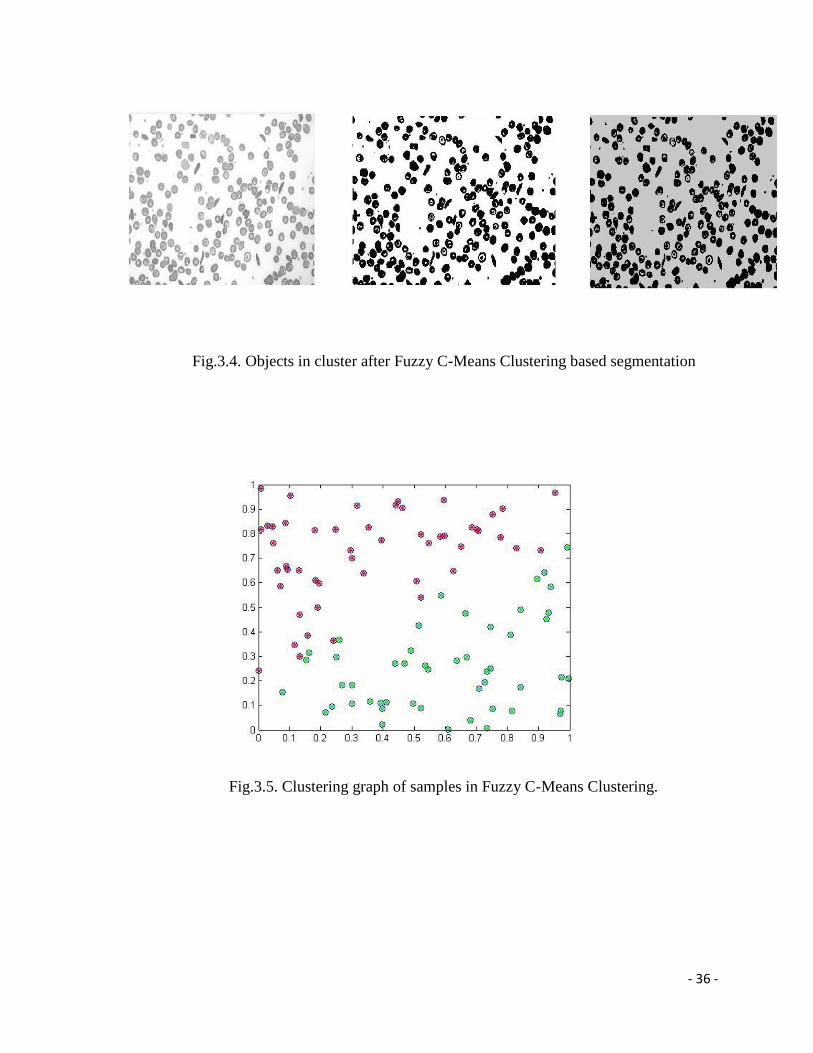
Fig.3.4. Objects in cluster after Fuzzy C-Means Clustering based segmentation

Fig.3.5. Clustering graph of samples in Fuzzy C-Means Clustering.

- 37 -

3.3 Feature Generation Processes

3.3.1. Geometrical Features Extraction

For unit cluster of k-means clustering based segmentation

Geometrical Features Normal

RBC

Sickle-

cell type-I

Sickle-cell

type-II

Anisopoikilocyte/Ovalocyte

Area 274 268 183 212

Perimeter 62.14 85.11 131.64 62.1

Centroid 15.6, 14.8 16, 17.2 15.4, 24.9 14.5, 15.0

Eccentricity 0.43 0.94 0.95 0.8

Major Axis Length 19.8 32.91 32.8 21.9

Minor Axis Length 17.8 11.1 10.2 13.1

Orientation 11.34 57.6 -74.5 -28.37

Equiv Diameter 18.7 18.47 15.3 16.4

Solidity 0.97 0.83 0.6 0.86

Extent 0.84 0.48 0.4 0.66

Mean 48.9 42.6 28.1 44.5

Aspect Ratio 0.9394 1.1935 1.6333 0.9667

Standard Deviation 76 68.5 54.6 69.6

Form Factor 0.9526 0.7149 0.6834 0.4872

Tab 1. Geometrical Features of K-Means Clusters

- 38 -

For unit cluster of fuzzy c-means clustering based segmentation

Geometrical Features Normal

RBC

Sickle-cell

type-I

Sickle-cell

type-II

Anisopoikilocyte/Ovalocyte

Area 420 512 708 506

Perimeter 78 88 110 86

Centroid 10.4, 11 10.4, 13.2 10.2, 19 12, 11.5

Eccentricity 0.3133 0.63 0.84 0.29

Major Axis Length 24.2 30 43.4 26.5

Minor Axis Length 23 23.1 23.9 25.4

Orientation 90 -88.7 89.6 0

Equiv Diameter 23.2 25.5 30 25.4

Solidity 1 0.98 0.96 1

Extent 1 0.98 0.96 1

Mean 210.45 219.2 226 220

Aspect Ratio 1.05 1.3 1.85 0.9565

Standard Deviation 37.8 44.4 42.2 31.73

Form Factor 0.9528 0.6535 0.7737 0.3628

3.3.2 Textural Features Extraction:

GLCM Results:

Tab 2. Geometrical Features of Fuzzy C-Means Clusters

- 39 -

For unit cluster of k-means clustering based segmentation

Textural Features Normal RBC Sickle-Cell I Sickle-Cell II Ovalocyte/

Anisopoikilocyte

Contrast 7.94e-02 9.03e-02 9.64e-02 1.08e-01

Correlation 8.05e-01 7.57e-01 5.72e-01 7.2e-01

Energy 5.18e-01 5.45e-01 6.87e-01 5.16e-01

Homogeneity 9.6e-01 9.54e-01 9.51e-01 9.45e-01

Entropy 0.34 0.28 0.39 0.28

For unit cluster of fuzzy c-means clustering based segmentation

Textural Features Normal RBC Sickle-Cell I Sickle-Cell II Ovalocyte/

Anisopoikilocyte

Contrast 0 2.91e-02 6.5e-02 0

Correlation NaN 1.1e-01 2.4e-01 NaN

Energy 1 9.3e-01 8.5e-01 1

Homogeneity 1 9.8e-01 9.6e-01 1

Entropy 2.76 2.76 2.76 2.76

Tab 3.Textural Features of K-Means Clusters

Tab 4. Textural Features of Fuzzy C-Means Clusters

- 40 -

Fig.3.6. GLCM Features Graph

- 41 -

3.3.3. Detecting Circles in an Image

3.4 Classification

After the various kinds of features were generated from the previous step, now they are used for

classifying the different kinds of red blood cells (RBC) present in the blood smear image. After

using proper grouping technique, we find that the form factor values extracted from the

geometrical features is of our great interest. For different values of form factor, cells are sorted

out as normal cell, sickle-cell, ovalocyte and anisopoikilocyte. Their numbers and the total

number of blood cells present in the smear are also calculated. For a normal blood cell, the value

of Form Factor nearly equals one.

Consequently, the cells in blood smear are categorized as follows:

Normal Cell Form Factor > 0.95

Sickle-Cell 0.6< Form Factor < 0.8

Ovalocyte/Anisopoikilocyte Form Factor < 0.5

Fig.3.7. Circles Recognition

- 42 -

Chapter 4: Conclusions and Future Study

The image processing techniques used in this project, which includes color altercation and

clustering based image segmentation has helped us to better understand the sickle-cells present in

Red Blood Cells (RBCs) in case of sickle-cell patient.

Using the image segmentation technique and the following sub-imaging technique, I can obtain

the images of particular affected RBCs, i.e. Sickle-cells, Anisopoikilocytes and Ovalocytes and

further apply feature extraction process to determine the characteristics of affected RBCs and

thus make an artificial neural network to automatically diagnose sickle-cells disease affected

person.

Chapter 5: References

[1] Gonzalez RG, RE Woods and SL Eddins, “Digital Image Processing”, Pearson

Education, Inc. NJ. 2007.

[2] Bernd Jahne. “Digital Image Processing”, Springer Publications, Berlin, 2011.

[3] Jain A. K., “Fundamentals of Digital Image Processing”. Pearson Education, 1st Indian

edition, 2003.

[4] Bacus J. W. and Weens J. H., “An automated method of differential red blood cell

classification with application to the diagnosis of anemia”, J Histochem Cytochem, 25: 614,

1977.

[5] Ross N. E., Pritchard C. J., Rubin D. M., Duse A. G. “Automated image processing

method for the diagnosis and classification of malaria on thin blood smears”, International

federation for Medical & Biomedical engineering, March 2006.

[6] Patra D. and Mohapatra S., “Automated Cell Nucleus Segmentation and Acute Leukemia

Detection in Blood Microscopic Images”, NIT Rourkela. 2010.

[7] Price-Jones C. “The diameter of red cells in pernicious anameia and in anameia following

haemorrhage”. J Pathol Bacteriol, 1992.

[8] Malone, BS, Werlin, SL. “Cholecystectomy and cholelithiasis in sickle cell anemia”. Am

J Dis Child; pp. 142:799, 1988.

[9] Al-Salem AH. “Indications and complications of splenectomy for children with sickle

cell disease”, J Pediatr Surg, Nov 2006.

- 43 -

[10] Aguilar C, Vichinsky E, Neumayr L. “Bone and Joint Disease in Sickle Cell Disease”,

Hematol Oncol Clin North Am.; 19(5):929-4, Oct 2005.

[11] Taylor, C, Carter, F, Poulose, J, Rolle, S, Babu, S, Crichlow, S. “Clinical presentation of

acute chest syndrome in sickle cell disease”. Postgrad. Med. J. 80: 346-349, 2004.

[12] McLaughlin V.V. and Channick R., “Sickle cell disease-associated pulmonary

hypertension: a coat of many colors”, Am J Respir Crit Care Med 175(12): 1218-9, 2007.

[13] Siddiqui A.K., Ahmed S.P., “Manifestations of Sickle Cell Disease”, Postgrad Med J.

Jul; 79(933):384-90. 2003

[14] Cochran RT, “Hyposthenuria in Sickle Cell”, Arch Intern Med.; 112:222-5. Aug 1963.

[15] Kato, G. J. and Gladwin M.T. “Deconstructing sickle cell disease: reappraisal of the role

of hemolysis in the development of clinical subphenotypes”. Blood Rev 21(1): 37-47, 2007.

[16] Wen-Xiong Kang, Qing-Qiang Yang, Run-Peng Liang., “The Comparative Research on

Image Segmentation Algorithms”, First International Workshop on Education Technology

and Computer Science, Coll. of Autom. Sci. & Eng., South China Univ. of Technol.,

Guangzhou, location Wuhan, Hubei. 2009.

[17] Comaniciu D. and Meer P, “Cell Image Segmentation for Diagnostic Pathology”. In J.

S. Suri, S. K. Setarehdan, and S. Singh, editors, “Advanced algorithmic approaches to

medical image segmentation: state-of-the-art application in cardiology, neurology,

mammography and pathology”, 541 –558. Springer, 2001.

[18] Coleman G.B. and Andrews H.C., “Image Segmentation by Clustering”. Proc. of the

IEEE, vol. 67, pp. 773-785, 1979.

[19] Ray S., Turi R.H. and Tisher P.E., “Clustering based colour image segmentation”,

Monash University, Australia, 2002.

[20] Krishnapuram R, Keller JM, “A possibilistic approach to clustering”. IEEE Trans Fuzzy

Syst; 1:98–110, 1993.

[21] Di Ruberto C., Dempster A., Khan S. and Jarra B., “Analysis of infected blood cell

images using morphological operators”. Image Vis Comput 20(2):133–146, 2002.

[22] Foley D.H., “Consideration of sample and feature size”. IEEE Trans Inform Theory IT-

18 618–626, 1972.

[23] Bacus J.W., “Design and performance of an automated leukocyte classifier”. In

Proceedings of the Second International conference on Pattern recognition, page 374, August

1974.

[24] Green J.E., “Computer methods for erythrocyte analysis”, In proceedings of the

Symposium of Feature Extraction and Selection in Pattern Recognition, page 100, October

1970.

[25] Yang Bai, Lihua Guo, Lianwen Jin, Qinghua Huang, “A novel feature extraction method

using pyramid histogram of orientation gradients for smile recognition”, 2008.

- 44 -

[26] Magudeeswaran V., Karthikeyan P. and Thirumurugan P., “Feature Extraction &

Classification of blood cells using artificial neural network”, PSNA College of Engineering,

Tamil Nadu, 2012.

[27] Haralick R.M., Shanmugam K., and Dinstein I., “Textural Features of Image

Classification”, IEEE Transactions on Systems, Man and Cybernetics, vol. SMC-3, no. 6,

Nov. 1973.

[28] The MathWorks, Inc., “Image Processing Toolbox – For Use with MATLAB,” The

MathWorks, Inc., 2012.

Road Map

Work List Deadline

Literature Review and System Overview 10th

March, 2013

Color Altercation and Clustering based image segmentation 5th

May, 2013

Feature Extraction Process 30th

May, 2013

Classification using Artificial Neural Network 15th

June, 2013